[M] Mata Reference Manual V13
User Manual:
Open the PDF directly: View PDF ![]() .
.
Page Count: 1005 [warning: Documents this large are best viewed by clicking the View PDF Link!]
- Contents
- [IG] Installation Guide
- Simple installation
- Installing Stata for Windows
- Installing Stata for Mac
- Installing Stata for Unix
- Installation overview
- Find your installation DVD and paper license
- Obtain superuser access
- Create a directory for Stata
- Upgrading
- Install Stata
- Initialize the license
- Set the message of the day (optional)
- Verify that Stata is working
- Modify shell start-up script
- Update Stata if necessary
- Starting Stata
- Exiting Stata
- Troubleshooting Unix installation
- Troubleshooting Unix start-up
- Stata(console) starts but Stata(GUI) does not
- Platforms and flavors
- Documentation
- [GS] Getting Started
- [GSM] Mac
- Contents
- 1 Introducing Stata---sample session
- 2 The Stata user interface
- 3 Using the Viewer
- The Viewer's purpose
- Viewer buttons
- Viewer's function
- Viewing local text files, including SMCL files
- Viewing remote files over the Internet
- Navigating within the Viewer
- Printing
- Tabs in the Viewer
- Right-clicking on the Viewer window
- Searching for help in the Viewer
- Commands in the Viewer
- Using the Viewer from the Command window
- 4 Getting help
- 5 Opening and saving Stata datasets
- 6 Using the Data Editor
- 7 Using the Variables Manager
- 8 Importing data
- 9 Labeling data
- 10 Listing data and basic command syntax
- 11 Creating new variables
- 12 Deleting variables and observations
- 13 Using the Do-file Editor---automating Stata
- 14 Graphing data
- 15 Editing graphs
- 16 Saving and printing results by using logs
- 17 Setting font and window preferences
- 18 Learning more about Stata
- 19 Updating and extending Stata---Internet functionality
- A Troubleshooting Stata
- B Advanced Stata usage
- C More on Stata for Mac
- Subject index
- [GSU] Unix
- Contents
- 1 Introducing Stata---sample session
- 2 The Stata user interface
- 3 Using the Viewer
- The Viewer in Stata(GUI)
- The Viewer's purpose
- Viewer buttons
- Viewer's function
- Viewing local text files, including SMCL files
- Viewing remote files over the Internet
- Navigating within the Viewer
- Printing
- Tabs in the Viewer
- Right-clicking on the Viewer window
- Searching for help in the Viewer
- Commands in the Viewer
- Using the Viewer from the Command window
- 4 Getting help
- 5 Opening and saving Stata datasets
- 6 Using the Data Editor
- 7 Using the Variables Manager
- 8 Importing data
- 9 Labeling data
- 10 Listing data and basic command syntax
- 11 Creating new variables
- 12 Deleting variables and observations
- 13 Using the Do-file Editor---automating Stata
- 14 Graphing data
- 15 Editing graphs
- 16 Saving and printing results by using logs
- 17 Setting font and window preferences
- 18 Learning more about Stata
- 19 Updating and extending Stata---Internet functionality
- A Troubleshooting Stata
- B Advanced Stata usage
- C Stata manual pages for Unix
- conren
- stata
- Subject index
- [GSW] Windows
- Contents
- 1 Introducing Stata---sample session
- 2 The Stata user interface
- 3 Using the Viewer
- The Viewer's purpose
- Viewer buttons
- Viewer's function
- Viewing local text files, including SMCL files
- Viewing remote files over the Internet
- Navigating within the Viewer
- Printing
- Tabs in the Viewer
- Right-clicking on the Viewer window
- Searching for help in the Viewer
- Commands in the Viewer
- Using the Viewer from the Command window
- 4 Getting help
- 5 Opening and saving Stata datasets
- 6 Using the Data Editor
- 7 Using the Variables Manager
- 8 Importing data
- 9 Labeling data
- 10 Listing data and basic command syntax
- 11 Creating new variables
- 12 Deleting variables and observations
- 13 Using the Do-file Editor---automating Stata
- 14 Graphing data
- 15 Editing graphs
- 16 Saving and printing results by using logs
- 17 Setting font and window preferences
- 18 Learning more about Stata
- 19 Updating and extending Stata---Internet functionality
- A Troubleshooting Stata
- B Advanced Stata usage
- C More on Stata for Windows
- Subject index
- [GSM] Mac
- [U] User's Guide
- Contents
- Stata basics
- Elements of Stata
- 11 Language syntax
- 12 Data
- 13 Functions and expressions
- 13.1 Overview
- 13.2 Operators
- 13.3 Functions
- 13.4 System variables (_variables)
- 13.5 Accessing coefficients and standard errors
- 13.6 Accessing results from Stata commands
- 13.7 Explicit subscripting
- 13.8 Indicator values for levels of factor variables
- 13.9 Time-series operators
- 13.10 Label values
- 13.11 Precision and problems therein
- 13.12 References
- 14 Matrix expressions
- 14.1 Overview
- 14.2 Row and column names
- 14.3 Vectors and scalars
- 14.4 Inputting matrices by hand
- 14.5 Accessing matrices created by Stata commands
- 14.6 Creating matrices by accumulating data
- 14.7 Matrix operators
- 14.8 Matrix functions
- 14.9 Subscripting
- 14.10 Using matrices in scalar expressions
- 14.11 Reference
- 15 Saving and printing output---log files
- 16 Do-files
- 17 Ado-files
- 17.1 Description
- 17.2 What is an ado-file?
- 17.3 How can I tell if a command is built in or an ado-file?
- 17.4 How can I look at an ado-file?
- 17.5 Where does Stata look for ado-files?
- 17.6 How do I install an addition?
- 17.7 How do I add my own ado-files?
- 17.8 How do I install official updates?
- 17.9 How do I install updates to user-written additions?
- 17.10 Reference
- 18 Programming Stata
- 18.1 Description
- 18.2 Relationship between a program and a do-file
- 18.3 Macros
- 18.4 Program arguments
- 18.5 Scalars and matrices
- 18.6 Temporarily destroying the data in memory
- 18.7 Temporary objects
- 18.8 Accessing results calculated by other programs
- 18.9 Accessing results calculated by estimation commands
- 18.10 Storing results
- 18.11 Ado-files
- 18.12 Tools for interacting with programs outside Stata and with other languages
- 18.13 A compendium of useful commands for programmers
- 18.14 References
- 19 Immediate commands
- 20 Estimation and postestimation commands
- 20.1 All estimation commands work the same way
- 20.2 Standard syntax
- 20.3 Replaying prior results
- 20.4 Cataloging estimation results
- 20.5 Saving estimation results
- 20.6 Specifying the estimation subsample
- 20.7 Specifying the width of confidence intervals
- 20.8 Formatting the coefficient table
- 20.9 Obtaining the variance--covariance matrix
- 20.10 Obtaining predicted values
- 20.11 Accessing estimated coefficients
- 20.12 Performing hypothesis tests on the coefficients
- 20.13 Obtaining linear combinations of coefficients
- 20.14 Obtaining nonlinear combinations of coefficients
- 20.15 Obtaining marginal means, adjusted predictions, and predictive margins
- 20.16 Obtaining conditional and average marginal effects
- 20.17 Obtaining pairwise comparisons
- 20.18 Obtaining contrasts, tests of interactions, and main effects
- 20.19 Graphing margins, marginal effects, and contrasts
- 20.20 Dynamic forecasts and simulations
- 20.21 Obtaining robust variance estimates
- 20.22 Obtaining scores
- 20.23 Weighted estimation
- 20.24 A list of postestimation commands
- 20.25 References
- Advice
- 21 Entering and importing data
- 22 Combining datasets
- 23 Working with strings
- 24 Working with dates and times
- 25 Working with categorical data and factor variables
- 26 Overview of Stata estimation commands
- 26.1 Introduction
- 26.2 Means, proportions, and related statistics
- 26.3 Linear regression with simple error structures
- 26.4 Structural equation modeling (SEM)
- 26.5 ANOVA, ANCOVA, MANOVA, and MANCOVA
- 26.6 Generalized linear models
- 26.7 Binary-outcome qualitative dependent-variable models
- 26.8 ROC analysis
- 26.9 Conditional logistic regression
- 26.10 Multiple-outcome qualitative dependent-variable models
- 26.11 Count dependent-variable models
- 26.12 Exact estimators
- 26.13 Linear regression with heteroskedastic errors
- 26.14 Stochastic frontier models
- 26.15 Regression with systems of equations
- 26.16 Models with endogenous sample selection
- 26.17 Models with time-series data
- 26.18 Panel-data models
- 26.19 Multilevel mixed-effects models
- 26.20 Survival-time (failure-time) models
- 26.21 Treatment-effect models
- 26.22 Generalized method of moments (GMM)
- 26.23 Estimation with correlated errors
- 26.24 Survey data
- 26.25 Multiple imputation
- 26.26 Multivariate and cluster analysis
- 26.27 Pharmacokinetic data
- 26.28 Specification search tools
- 26.29 Power and sample-size analysis
- 26.30 Obtaining new estimation commands
- 26.31 References
- 27 Commands everyone should know
- 28 Using the Internet to keep up to date
- Subject and author index
- [D] Data Management
- Contents
- intro
- data management
- append
- assert
- bcal
- by
- cd
- cf
- changeeol
- checksum
- clear
- clonevar
- codebook
- collapse
- compare
- compress
- contract
- copy
- corr2data
- count
- cross
- data types
- datasignature
- datetime
- Syntax
- Types of dates and their human readable forms (HRFs)
- Stata internal form (SIF)
- HRF-to-SIF conversion functions
- Displaying SIFs in HRF
- Building SIFs from components
- SIF-to-SIF conversion
- Extracting time-of-day components from SIFs
- Extracting date components from SIFs
- Conveniently typing SIF values
- Obtaining and working with durations
- Using dates and times from other software
- Description
- Remarks and examples
- References
- Also see
- Syntax
- datetime business calendars
- datetime business calendars creation
- Syntax
- Description
- Remarks and examples
- Introduction
- Concepts
- The preliminary commands
- The omit commands: from/to and if
- The omit commands: and
- The omit commands: omit date
- The omit commands: omit dayofweek
- The omit commands: omit dowinmonth
- Creating stbcal-files with bcal create
- Where to place stbcal-files
- How to debug stbcal-files
- Ideas for calendars that may not occur to you
- Also see
- datetime display formats
- datetime translation
- Syntax
- Description
- Remarks and examples
- Introduction
- Specifying the mask
- How the HRF-to-SIF functions interpret the mask
- Working with two-digit years
- Working with incomplete dates and times
- Translating run-together dates, such as 20060125
- Valid times
- The clock() and Clock() functions
- Why there are two SIF datetime encodings
- Advice on using datetime/c and datetime/C
- Determining when leap seconds occurred
- The date() function
- The other translation functions
- Also see
- describe
- destring
- dir
- drawnorm
- drop
- ds
- duplicates
- edit
- egen
- encode
- erase
- expand
- expandcl
- export
- filefilter
- fillin
- format
- functions
- Description
- Mathematical functions
- Probability distributions and density functions
- Beta and noncentral beta distributions
- ibeta()
- betaden()
- ibetatail()
- invibeta()
- invibetatail()
- nibeta()
- invnibeta()
- Binomial distribution
- binomial()
- binomialp()
- binomialtail()
- invbinomial()
- invbinomialtail()
- Chi-squared and noncentral chi-squared distributions
- chi2()
- chi2den()
- chi2tail()
- invchi2()
- invchi2tail()
- nchi2()
- nchi2den()
- nchi2tail()
- invnchi2()
- invnchi2tail()
- npnchi2()
- Dunnett's multiple range distribution
- dunnettprob()
- invdunnettprob()
- F and noncentral F distributions
- F()
- Fden()
- Ftail()
- invF()
- invFtail()
- nF()
- nFtail()
- invnFtail()
- npnF()
- Gamma distribution
- gammap()
- gammaden()
- gammaptail()
- invgammap()
- invgammaptail()
- dgammapda()
- dgammapdada()
- dgammapdadx()
- dgammapdx()
- dgammapdxdx()
- Hypergeometric distribution
- hypergeometric()
- hypergeometricp()
- Negative binomial distribution
- nbinomial()
- nbinomialp()
- nbinomialtail()
- invnbinomial()
- invnbinomiailtail()
- Normal (Gaussian), log of the normal, and binormal distributions
- binormal()
- normal()
- normalden()
- invnormal()
- lnnormal()
- Poisson distribution
- poisson()
- poissonp()
- poissontail()
- invpoisson()
- invpoissontail()
- Student's t and noncentral Student's t distributions
- t()
- tden()
- ttail()
- invt()
- invttail()
- nt()
- ntden()
- nttail()
- invnttail()
- npnt()
- Tukey's Studentized range distribution
- tukeyprob()
- invtukeyprob()
- Random-number functions
- String functions
- abbrev()
- char()
- indexnot()
- itrim()
- length()
- lower()
- ltrim()
- plural()
- proper()
- real()
- regexm()
- regexr()
- regexs()
- reverse()
- rtrim()
- soundex()
- soundex_nara()
- strcat()
- strdup()
- string()
- strlen()
- strlower()
- strltrim()
- strmatch()
- strofreal()
- strpos()
- strproper()
- strreverse()
- strrtrim()
- strtoname()
- strtrim()
- strupper()
- subinstr()
- subinword()
- substr()
- trim()
- upper()
- word()
- wordcount()
- Programming functions
- autocode()
- byteorder()
- c()
- _caller()
- chop()
- clip()
- cond()
- e()
- e(sample)
- epsdouble()
- epsfloat()
- fileexists()
- fileread()
- filereaderror()
- filewrite()
- float()
- fmtwidth()
- has_eprop()
- inlist()
- inrange()
- irecode()
- matrix()
- maxbyte()
- maxdouble()
- maxfloat()
- maxint()
- maxlong()
- mi()
- minbyte()
- mindouble()
- minfloat()
- minint()
- minlong()
- missing()
- r()
- recode()
- replay()
- return()
- s()
- scalar()
- smallestdouble()
- Date and time functions
- bofd()
- Cdhms()
- clock()
- Cmdyhms()
- Cofc()
- cofC()
- Cofd()
- cofd()
- daily()
- date()
- day()
- dhms()
- dofb()
- dofC()
- dofc()
- dofh()
- dofm()
- dofq()
- dofw()
- dofy()
- dow()
- doy()
- halfyear()
- halfyearly()
- hh()
- hhC()
- hms()
- hofd()
- hours()
- mdy()
- mdyhms()
- minutes()
- mm()
- mmC()
- mofd()
- month()
- monthly()
- msofhours()
- msofminutes()
- msofseconds()
- qofd()
- quarter()
- quarterly()
- seconds()
- ss()
- ssC()
- tC()
- tc()
- td()
- th()
- tm()
- tq()
- tw()
- week()
- weekly()
- wofd()
- year()
- yearly()
- yh()
- ym()
- yofd()
- yq()
- yw()
- Selecting time spans
- Matrix functions returning a matrix
- Matrix functions returning a scalar
- Acknowledgments
- References
- Also see
- Description
- generate
- gsort
- hexdump
- icd9
- import
- import delimited
- import excel
- import haver
- import sasxport
- infile (fixed format)
- infile (free format)
- infix (fixed format)
- input
- inspect
- ipolate
- isid
- joinby
- label
- label language
- labelbook
- list
- lookfor
- memory
- merge
- missing values
- mkdir
- mvencode
- notes
- obs
- odbc
- order
- outfile
- pctile
- putmata
- range
- recast
- recode
- rename
- rename group
- reshape
- Syntax
- Menu
- Description
- Options
- Remarks and examples
- Description of basic syntax
- Wide and long data forms
- Avoiding and correcting mistakes
- reshape long and reshape wide without arguments
- Missing variables
- Advanced issues with basic syntax: i()
- Advanced issues with basic syntax: j()
- Advanced issues with basic syntax: xij
- Advanced issues with basic syntax: String identifiers for j()
- Advanced issues with basic syntax: Second-level nesting
- Description of advanced syntax
- Stored results
- Acknowledgment
- References
- Also see
- rmdir
- sample
- save
- separate
- shell
- snapshot
- sort
- split
- stack
- statsby
- sysuse
- type
- use
- varmanage
- webuse
- xmlsave
- xpose
- zipfile
- Subject and author index
- [G] Graphics
- Contents
- Introduction
- Commands
- graph
- graph bar
- Syntax
- Menu
- Description
- Options
- Remarks and examples
- Introduction
- Examples of syntax
- Treatment of bars
- Treatment of data
- Multiple bars (overlapping the bars)
- Controlling the text of the legend
- Multiple over()s (repeating the bars)
- Nested over()s
- Charts with many categories
- How bars are ordered
- Reordering the bars
- Putting the bars in a prespecified order
- Putting the bars in height order
- Putting the bars in a derived order
- Reordering the bars, example
- Use with by()
- Video example
- History
- References
- Also see
- graph box
- graph combine
- graph copy
- graph describe
- graph dir
- graph display
- graph dot
- graph drop
- graph export
- graph manipulation
- graph matrix
- graph other
- graph pie
- graph play
- graph print
- graph query
- graph rename
- graph save
- graph set
- graph twoway
- graph twoway area
- graph twoway bar
- graph twoway connected
- graph twoway contour
- graph twoway contourline
- graph twoway dot
- graph twoway dropline
- graph twoway fpfit
- graph twoway fpfitci
- graph twoway function
- graph twoway histogram
- graph twoway kdensity
- graph twoway lfit
- graph twoway lfitci
- graph twoway line
- graph twoway lowess
- graph twoway lpoly
- graph twoway lpolyci
- graph twoway mband
- graph twoway mspline
- graph twoway pcarrow
- graph twoway pcarrowi
- graph twoway pccapsym
- graph twoway pci
- graph twoway pcscatter
- graph twoway pcspike
- graph twoway qfit
- graph twoway qfitci
- graph twoway rarea
- graph twoway rbar
- graph twoway rcap
- graph twoway rcapsym
- graph twoway rconnected
- graph twoway rline
- graph twoway rscatter
- graph twoway rspike
- graph twoway scatter
- Syntax
- Menu
- Description
- Options
- Remarks and examples
- Typical use
- Scatter syntax
- The overall look for the graph
- The size and aspect ratio of the graph
- Titles
- Axis titles
- Axis labels and ticking
- Grid lines
- Added lines
- Axis range
- Log scales
- Multiple axes
- Markers
- Weighted markers
- Jittered markers
- Connected lines
- Graphs by groups
- Saving graphs
- Video example
- Appendix: Styles and composite styles
- References
- Also see
- graph twoway scatteri
- graph twoway spike
- graph twoway tsline
- graph use
- palette
- set graphics
- set printcolor
- set scheme
- Options
- added_line_options
- added_text_options
- addplot_option
- advanced_options
- area_options
- aspect_option
- axis_choice_options
- Syntax
- Description
- Options
- Remarks and examples
- Usual case: one set of axes
- Special case: multiple axes due to multiple scales
- yaxis(1) and xaxis(1) are the defaults
- Notation style is irrelevant
- yaxis() and xaxis() are plot options
- Specifying the other axes options with multiple axes
- Each plot may have at most one x scale and one y scale
- Special case: Multiple axes with a shared scale
- Reference
- Also see
- axis_label_options
- axis_options
- axis_scale_options
- axis_title_options
- barlook_options
- blabel_option
- by_option
- cat_axis_label_options
- cat_axis_line_options
- clegend_option
- cline_options
- connect_options
- eps_options
- fcline_options
- fitarea_options
- legend_options
- line_options
- marker_label_options
- marker_options
- name_option
- nodraw_option
- play_option
- png_options
- pr_options
- ps_options
- rcap_options
- region_options
- rspike_options
- saving_option
- scale_option
- scheme_option
- std_options
- textbox_options
- tif_options
- title_options
- twoway_options
- Styles/concepts/schemes
- addedlinestyle
- alignmentstyle
- anglestyle
- areastyle
- axisstyle
- bystyle
- clockposstyle
- colorstyle
- compassdirstyle
- concept: gph files
- concept: lines
- concept: repeated options
- connectstyle
- gridstyle
- intensitystyle
- justificationstyle
- legendstyle
- linepatternstyle
- linestyle
- linewidthstyle
- marginstyle
- markerlabelstyle
- markersizestyle
- markerstyle
- orientationstyle
- plotregionstyle
- pstyle
- relativesize
- ringposstyle
- schemes intro
- scheme economist
- scheme s1
- scheme s2
- scheme sj
- shadestyle
- stylelists
- symbolstyle
- text
- textboxstyle
- textsizestyle
- textstyle
- ticksetstyle
- tickstyle
- Subject and author index
- [ME] Multilevel Mixed Effects
- Contents
- me
- mecloglog
- mecloglog postestimation
- meglm
- meglm postestimation
- melogit
- melogit postestimation
- menbreg
- menbreg postestimation
- meologit
- meologit postestimation
- meoprobit
- meoprobit postestimation
- mepoisson
- mepoisson postestimation
- meprobit
- meprobit postestimation
- meqrlogit
- meqrlogit postestimation
- meqrpoisson
- meqrpoisson postestimation
- mixed
- Syntax
- Menu
- Description
- Options
- Remarks and examples
- Introduction
- Two-level models
- Covariance structures
- Likelihood versus restricted likelihood
- Three-level models
- Blocked-diagonal covariance structures
- Heteroskedastic random effects
- Heteroskedastic residual errors
- Other residual-error structures
- Crossed-effects models
- Diagnosing convergence problems
- Survey data
- Stored results
- Methods and formulas
- Acknowledgments
- References
- Also see
- mixed postestimation
- Glossary
- Subject and author index
- [MI] Multiple Imputation
- Contents
- intro substantive
- intro
- estimation
- mi add
- mi append
- mi convert
- mi copy
- mi describe
- mi erase
- mi estimate
- Syntax
- Menu
- Description
- Options
- Remarks and examples
- Using mi estimate
- Example 1: Completed-data logistic analysis
- Example 2: Completed-data linear regression analysis
- Example 3: Completed-data survival analysis
- Example 4: Panel data and multilevel models
- Example 5: Estimating transformations
- Example 6: Monte Carlo error estimates
- Potential problems that can arise when using mi estimate
- Stored results
- Methods and formulas
- Acknowledgments
- References
- Also see
- mi estimate using
- mi estimate postestimation
- mi expand
- mi export
- mi export ice
- mi export nhanes1
- mi extract
- mi import
- mi import flong
- mi import flongsep
- mi import ice
- mi import nhanes1
- mi import wide
- mi impute
- Syntax
- Menu
- Description
- Options
- Remarks and examples
- Stored results
- Methods and formulas
- References
- Also see
- mi impute chained
- mi impute intreg
- mi impute logit
- mi impute mlogit
- mi impute monotone
- mi impute mvn
- mi impute nbreg
- mi impute ologit
- mi impute pmm
- mi impute poisson
- mi impute regress
- mi impute truncreg
- mi merge
- mi misstable
- mi passive
- mi predict
- Syntax
- Menu
- Description
- Options
- Remarks and examples
- Introduction
- Using mi predict and mi predictnl
- Example 1: Obtain MI linear predictions and other statistics
- Example 2: Obtain MI linear predictions for the estimation sample
- Example 3: Obtain MI estimates of probabilities
- Example 4: Obtain other MI predictions
- Example 5: Obtain MI predictions after multiple-equation commands
- Methods and formulas
- References
- Also see
- mi ptrace
- mi rename
- mi replace0
- mi reset
- mi reshape
- mi select
- mi set
- mi stsplit
- mi test
- mi update
- mi varying
- mi xeq
- mi XXXset
- noupdate option
- styles
- technical
- Description
- Remarks and examples
- Notation
- Definition of styles
- Adding new commands to mi
- Outline for new commands
- Utility routines
- u_mi_assert_set
- u_mi_certify_data
- u_mi_no_sys_vars and u_mi_no_wide_vars
- u_mi_zap_chars
- u_mi_xeq_on_tmp_flongsep
- u_mi_get_flongsep_tmpname
- mata: u_mi_flongsep_erase()
- u_mi_sortback
- u_mi_save and u_mi_use
- mata: u_mi_wide_swapvars()
- u_mi_fixchars
- mata: u_mi_cpchars_get() and mata: u_mi_cpchars_put()
- mata: u_mi_get_mata_instanced_var()
- mata: u_mi_ptrace_*()
- How to write other set commands to work with mi
- Also see
- workflow
- Glossary
- Subject and author index
- [MV] Multivariate Statistics
- Contents
- intro
- multivariate
- alpha
- biplot
- ca
- ca postestimation
- ca postestimation plots
- candisc
- canon
- canon postestimation
- cluster
- Syntax
- Description
- Remarks and examples
- Introduction to cluster analysis
- Stata's cluster-analysis system
- Data transformations and variable selection
- Similarity and dissimilarity measures
- Partition cluster-analysis methods
- Hierarchical cluster-analysis methods
- Hierarchical cluster analysis applied to a dissimilarity matrix
- Postclustering commands
- Cluster-management tools
- References
- Also see
- clustermat
- cluster dendrogram
- cluster generate
- cluster kmeans and kmedians
- cluster linkage
- cluster notes
- cluster programming subroutines
- cluster programming utilities
- cluster stop
- cluster utility
- discrim
- discrim estat
- discrim knn
- discrim knn postestimation
- discrim lda
- discrim lda postestimation
- discrim logistic
- discrim logistic postestimation
- discrim qda
- discrim qda postestimation
- factor
- factor postestimation
- hotelling
- manova
- manova postestimation
- matrix dissimilarity
- mca
- mca postestimation
- mca postestimation plots
- mds
- mds postestimation
- mds postestimation plots
- mdslong
- mdsmat
- measure_option
- mvreg
- mvreg postestimation
- mvtest
- mvtest correlations
- mvtest covariances
- mvtest means
- mvtest normality
- pca
- pca postestimation
- procrustes
- procrustes postestimation
- rotate
- rotatemat
- scoreplot
- screeplot
- Glossary
- Subject and author index
- [PSS] Power and Sample Size
- Contents
- intro
- GUI
- power
- power, graph
- power, table
- power onemean
- power twomeans
- power pairedmeans
- power oneproportion
- power twoproportions
- power pairedproportions
- power onevariance
- power twovariances
- power onecorrelation
- power twocorrelations
- power oneway
- power twoway
- power repeated
- unbalanced designs
- Glossary
- Subject and author index
- [R] Base Reference
- Contents
- Introduction
- A
- about
- adoupdate
- ameans
- anova
- anova postestimation
- areg
- areg postestimation
- asclogit
- asclogit postestimation
- asmprobit
- asmprobit postestimation
- asroprobit
- asroprobit postestimation
- B
- C
- centile
- ci
- clogit
- clogit postestimation
- cloglog
- cloglog postestimation
- cls
- cnsreg
- cnsreg postestimation
- constraint
- contrast
- Syntax
- Menu
- Description
- Options
- Remarks and examples
- Stored results
- Methods and formulas
- References
- Also see
- contrast postestimation
- copyright
- copyright apache
- copyright boost
- copyright freetype
- copyright icu
- copyright jagpdf
- copyright lapack
- copyright libpng
- copyright miglayout
- copyright scintilla
- copyright ttf2pt1
- copyright zlib
- correlate
- cumul
- cusum
- D
- E
- eform_option
- eivreg
- eivreg postestimation
- error messages
- esize
- estat
- estat classification
- estat gof
- estat ic
- estat summarize
- estat vce
- estimates
- estimates describe
- estimates for
- estimates notes
- estimates replay
- estimates save
- estimates stats
- estimates store
- estimates table
- estimates title
- estimation options
- exit
- exlogistic
- exlogistic postestimation
- expoisson
- expoisson postestimation
- F
- G
- gllamm
- glm
- glm postestimation
- glogit
- glogit postestimation
- gmm
- Syntax
- Menu
- Description
- Options
- Remarks and examples
- Introduction
- Substitutable expressions
- The weight matrix and two-step estimation
- Obtaining standard errors
- Exponential (Poisson) regression models
- Specifying derivatives
- Exponential regression models with panel data
- Rational-expectations models
- System estimators
- Dynamic panel-data models
- Details of moment-evaluator programs
- Stored results
- Methods and formulas
- References
- Also see
- gmm postestimation
- grmeanby
- H
- hausman
- heckman
- heckman postestimation
- heckoprobit
- heckoprobit postestimation
- heckprobit
- heckprobit postestimation
- help
- hetprobit
- hetprobit postestimation
- histogram
- I
- icc
- inequality
- intreg
- intreg postestimation
- ivpoisson
- ivpoisson postestimation
- ivprobit
- ivprobit postestimation
- ivregress
- ivregress postestimation
- ivtobit
- ivtobit postestimation
- J
- K
- L
- ladder
- level
- limits
- lincom
- linktest
- lnskew0
- log
- logistic
- logistic postestimation
- Description
- Syntax for predict
- Menu for predict
- Options for predict
- Remarks and examples
- predict without options
- predict with the xb and stdp options
- predict with the residuals option
- predict with the number option
- predict with the deviance option
- predict with the rstandard option
- predict with the hat option
- predict with the dx2 option
- predict with the ddeviance option
- predict with the dbeta option
- Methods and formulas
- References
- Also see
- logit
- logit postestimation
- loneway
- lowess
- lpoly
- lroc
- lrtest
- lsens
- lv
- M
- margins
- Syntax
- Menu
- Description
- Options
- Remarks and examples
- Introduction
- Obtaining margins of responses
- Example 1: A simple case after regress
- Example 2: A simple case after logistic
- Example 3: Average response versus response at average
- Example 4: Multiple margins from one command
- Example 5: Margins with interaction terms
- Example 6: Margins with continuous variables
- Example 7: Margins of continuous variables
- Example 8: Margins of interactions
- Example 9: Decomposing margins
- Example 10: Testing margins---contrasts of margins
- Example 11: Margins of a specified prediction
- Example 12: Margins of a specified expression
- Example 13: Margins with multiple outcomes (responses)
- Example 14: Margins with multiple equations
- Example 15: Margins evaluated out of sample
- Obtaining margins of derivatives of responses (a.k.a. marginal effects)
- Do not specify marginlist when you mean over()
- Use at() freely, especially with continuous variables
- Expressing derivatives as elasticities
- Derivatives versus discrete differences
- Example 16: Average marginal effect (partial effects)
- Example 17: Average marginal effect of all covariates
- Example 18: Evaluating marginal effects over the response surface
- Obtaining margins with survey data and representative samples
- Standardizing margins
- Obtaining margins as though the data were balanced
- Obtaining margins with nested designs
- Special topics
- Video examples
- Glossary
- Stored results
- Methods and formulas
- References
- Also see
- margins postestimation
- margins, contrast
- margins, pwcompare
- marginsplot
- Syntax
- Menu
- Description
- Options
- Remarks and examples
- Introduction
- Dataset
- Profile plots
- Interaction plots
- Contrasts of margins---effects (discrete marginal effects)
- Three-way interactions
- Continuous covariates
- Plots at every value of a continuous covariate
- Contrasts of at() groups---discrete effects
- Controlling the graph's dimensions
- Pairwise comparisons
- Horizontal is sometimes better
- Marginal effects
- Plotting a subset of the results from margins
- Advanced usage
- Video examples
- Addendum: Advanced uses of dimlist
- Acknowledgments
- References
- Also see
- matsize
- maximize
- mean
- mean postestimation
- meta
- mfp
- mfp postestimation
- misstable
- mkspline
- ml
- Syntax
- Description
- Options
- Options for use with ml model in interactive or noninteractive mode
- Options for use with ml model in noninteractive mode
- Options for use when specifying equations
- Options for use with ml search
- Option for use with ml plot
- Options for use with ml init
- Options for use with ml maximize
- Option for use with ml graph
- Options for use with ml display
- Options for use with mleval
- Option for use with mlsum
- Option for use with mlvecsum
- Option for use with mlmatsum
- Options for use with mlmatbysum
- Options for use with ml score
- Remarks and examples
- Stored results
- Methods and formulas
- References
- Also see
- mlexp
- mlexp postestimation
- mlogit
- mlogit postestimation
- more
- mprobit
- mprobit postestimation
- margins
- N
- nbreg
- nbreg postestimation
- nestreg
- net
- Syntax
- Description
- Options
- Remarks and examples
- Definition of a package
- The purpose of the net and ado commands
- Content pages
- Package-description pages
- Where packages are installed
- A summary of the net command
- A summary of the ado command
- Relationship of net and ado to the point-and-click interface
- Creating your own site
- Format of content and package-description files
- Example 1
- Example 2
- Additional package directives
- SMCL in content and package-description files
- Error-free file delivery
- References
- Also see
- net search
- netio
- news
- nl
- nl postestimation
- nlcom
- nlogit
- nlogit postestimation
- nlsur
- nlsur postestimation
- nptrend
- O
- P
- pcorr
- permute
- pk
- pkcollapse
- pkcross
- pkequiv
- pkexamine
- pkshape
- pksumm
- poisson
- poisson postestimation
- predict
- predictnl
- probit
- probit postestimation
- proportion
- proportion postestimation
- prtest
- pwcompare
- Syntax
- Menu
- Description
- Options
- Remarks and examples
- Stored results
- Methods and formulas
- References
- Also see
- pwcompare postestimation
- pwmean
- pwmean postestimation
- Q
- R
- ranksum
- ratio
- ratio postestimation
- reg3
- reg3 postestimation
- regress
- regress postestimation
- Description
- Predictions
- DFBETA influence statistics
- Tests for violation of assumptions
- Syntax for estat hettest
- Menu for estat
- Description for estat hettest
- Options for estat hettest
- Syntax for estat imtest
- Menu for estat
- Description for estat imtest
- Options for estat imtest
- Syntax for estat ovtest
- Menu for estat
- Description for estat ovtest
- Option for estat ovtest
- Syntax for estat szroeter
- Menu for estat
- Description for estat szroeter
- Options for estat szroeter
- Remarks and examples for estat hettest, estat imtest, estat ovtest, and estat szroeter
- Stored results for estat hettest, estat imtest, and estat ovtest
- Variance inflation factors
- Measures of effect size
- Methods and formulas
- Acknowledgments
- References
- Also see
- regress postestimation diagnostic plots
- regress postestimation time series
- #review
- roc
- roccomp
- rocfit
- rocfit postestimation
- rocreg
- rocreg postestimation
- rocregplot
- roctab
- rologit
- rologit postestimation
- rreg
- rreg postestimation
- runtest
- S
- T
- U
- V
- W
- X
- Z
- Author index
- Subject index
- [SEM] Structural Equation Modeling
- Contents
- Acknowledgments
- intro 1
- intro 2
- Description
- Remarks and examples
- Using path diagrams to specify standard linear SEMs
- Specifying correlation
- Using the command language to specify standard linear SEMs
- Specifying generalized SEMs: Family and link
- Specifying generalized SEMs: Family and link, multinomial logistic regression
- Specifying generalized SEMs: Family and link, paths from response variables
- Specifying generalized SEMs: Multilevel mixed effects (2 levels)
- Specifying generalized SEMs: Multilevel mixed effects (3 levels)
- Specifying generalized SEMs: Multilevel mixed effects (4+ levels)
- Specifying generalized SEMs: Multilevel mixed effects with random intercepts
- Specifying generalized SEMs: Multilevel mixed effects with random slopes
- Reference
- Also see
- intro 3
- intro 4
- Description
- Remarks and examples
- Differences in assumptions between sem and gsem
- sem: Choice of estimation method
- gsem: Choice of estimation method
- Treatment of missing values
- Variable types: Observed, latent, endogenous, exogenous, and error
- Constraining parameters
- Identification 1: Substantive issues
- Identification 2: Normalization constraints (anchoring)
- References
- Also see
- intro 5
- Description
- Remarks and examples
- Single-factor measurement models
- Item--response theory (IRT) models
- Multiple-factor measurement models
- Confirmatory factor analysis (CFA) models
- Structural models 1: Linear regression
- Structural models 2: Gamma regression
- Structural models 3: Binary-outcome models
- Structural models 4: Count models
- Structural models 5: Ordinal models
- Structural models 6: Multinomial logistic regression
- Structural models 7: Dependencies between response variables
- Structural models 8: Unobserved inputs, outputs, or both
- Structural models 9: MIMIC models
- Structural models 10: Seemingly unrelated regression (SUR)
- Structural models 11: Multivariate regression
- Structural models 12: Mediation models
- Correlations
- Higher-order CFA models
- Correlated uniqueness model
- Latent growth models
- Models with reliability
- Multilevel mixed-effects models
- References
- Also see
- intro 6
- Description
- Remarks and examples
- The generic SEM model
- Fitting the model for different groups of the data
- Which parameters vary by default, and which do not
- Specifying which parameters are allowed to vary in broad, sweeping terms
- Adding constraints for path coefficients across groups
- Adding constraints for means, variances, or covariances across groups
- Adding constraints for some groups but not others
- Adding paths for some groups but not others
- Relaxing constraints
- Reference
- Also see
- intro 7
- Description
- Remarks and examples
- Replaying the model (sem and gsem)
- Displaying odds ratios, incidence-rate ratios, etc. (gsem only)
- Obtaining goodness-of-fit statistics (sem and gsem)
- Performing tests for including omitted paths and relaxing constraints (sem only)
- Performing tests of model simplification (sem and gsem)
- Displaying other results, statistics, and tests (sem and gsem)
- Obtaining predicted values (sem)
- Obtaining predicted values (gsem)
- Using contrast, pwcompare, and margins (sem and gsem)
- Accessing stored results
- Also see
- intro 8
- intro 9
- intro 10
- intro 11
- intro 12
- Description
- Remarks and examples
- Is your model identified?
- Convergence solutions generically described
- Temporarily eliminate option reliability()
- Use default normalization constraints
- Temporarily eliminate feedback loops
- Temporarily simplify the model
- Try other numerical integration methods (gsem only)
- Get better starting values (sem and gsem)
- Get better starting values (gsem)
- Also see
- Builder
- Builder, generalized
- estat eform
- estat eqgof
- estat eqtest
- estat framework
- estat ggof
- estat ginvariant
- estat gof
- estat mindices
- estat residuals
- estat scoretests
- estat stable
- estat stdize
- estat summarize
- estat teffects
- example 1
- example 2
- example 3
- example 4
- example 5
- example 6
- example 7
- example 8
- example 9
- example 10
- example 11
- example 12
- example 13
- example 14
- example 15
- example 16
- example 17
- example 18
- example 19
- example 20
- example 21
- example 22
- example 23
- example 24
- example 25
- example 26
- example 27g
- example 28g
- example 29g
- example 30g
- example 31g
- example 32g
- example 33g
- example 34g
- example 35g
- example 36g
- example 37g
- example 38g
- Description
- Remarks and examples
- Random-intercept model, single-equation formulation
- Random-intercept model, within-and-between formulation
- Random-slope model, single-equation formulation
- Random-slope model, within-and-between formulation
- Fitting the random-intercept model with the Builder
- Fitting the random-slope model with the Builder
- Reference
- Also see
- example 39g
- example 40g
- example 41g
- example 42g
- example 43g
- example 44g
- example 45g
- example 46g
- gsem
- gsem estimation options
- gsem family-and-link options
- gsem model description options
- gsem path notation extensions
- gsem postestimation
- gsem reporting options
- lincom
- lrtest
- methods and formulas for gsem
- methods and formulas for sem
- nlcom
- predict after gsem
- predict after sem
- sem
- sem and gsem option constraints()
- sem and gsem option covstructure()
- sem and gsem option from()
- sem and gsem option reliability()
- sem and gsem path notation
- sem and gsem syntax options
- sem estimation options
- sem group options
- sem model description options
- sem option method()
- sem option noxconditional
- sem option select()
- sem path notation extensions
- sem postestimation
- sem reporting options
- sem ssd options
- ssd
- test
- testnl
- Glossary
- Subject and author index
- [ST] Survival Analysis
- Contents
- intro
- survival analysis
- Description
- Remarks and examples
- Introduction
- Declaring and converting count data
- Converting snapshot data
- Declaring and summarizing survival-time data
- Manipulating survival-time data
- Obtaining summary statistics, confidence intervals, tables, etc.
- Fitting regression models
- Sample size and power determination for survival analysis
- Converting survival-time data
- Programmer's utilities
- Epidemiological tables
- Reference
- Also see
- ct
- ctset
- cttost
- discrete
- epitab
- Syntax
- Menu
- Description
- Options
- Remarks and examples
- Incidence-rate data
- Stratified incidence-rate data
- Standardized estimates with stratified incidence-rate data
- Cumulative incidence data
- Stratified cumulative incidence data
- Standardized estimates with stratified cumulative incidence data
- Case--control data
- Stratified case--control data
- Case--control data with multiple levels of exposure
- Case--control data with confounders and possibly multiple levels of exposure
- Standardized estimates with stratified case--control data
- Matched case--control data
- Video examples
- Stored results
- Methods and formulas
- Unstratified incidence-rate data (ir and iri)
- Unstratified cumulative incidence data (cs and csi)
- Unstratified case--control data (cc and cci)
- Unstratified matched case--control data (mcc and mcci)
- Stratified incidence-rate data (ir with the by() option)
- Stratified cumulative incidence data (cs with the by() option)
- Stratified case--control data (cc with by() option, mhodds, tabodds)
- Acknowledgments
- References
- Also see
- ltable
- snapspan
- st
- st_is
- stbase
- stci
- stcox
- Syntax
- Menu
- Description
- Options
- Remarks and examples
- Cox regression with uncensored data
- Cox regression with censored data
- Treatment of tied failure times
- Cox regression with discrete time-varying covariates
- Cox regression with continuous time-varying covariates
- Robust estimate of variance
- Cox regression with multiple-failure data
- Stratified estimation
- Cox regression as Poisson regression
- Cox regression with shared frailty
- Stored results
- Methods and formulas
- Acknowledgment
- References
- Also see
- stcox PH-assumption tests
- stcox postestimation
- stcrreg
- stcrreg postestimation
- stcurve
- stdescribe
- stfill
- stgen
- stir
- stpower
- stpower cox
- stpower exponential
- Syntax
- Menu
- Description
- Options
- Remarks and examples
- Introduction
- Other ways of specifying the effect size
- Sample-size determination by using different approximations
- Sample-size determination in the presence of censoring
- Nonuniform accrual and exponential losses to follow-up
- The conditional versus unconditional approaches
- Link to the sample-size and power computation for the log-rank test
- Power determination
- Stored results
- Methods and formulas
- References
- Also see
- stpower logrank
- stptime
- strate
- streg
- streg postestimation
- sts
- sts generate
- sts graph
- sts list
- sts test
- stset
- Syntax
- Menu
- Description
- Options for use with stset and streset
- Options unique to streset
- Options for st
- Remarks and examples
- What are survival-time data?
- Key concepts
- Survival-time datasets
- Using stset
- Two concepts of time
- The substantive meaning of analysis time
- Setting the failure event
- Setting multiple failures
- First entry times
- Final exit times
- Intermediate exit and reentry times (gaps)
- if() versus if exp
- Past and future records
- Using streset
- Performance and multiple-record-per-subject datasets
- Sequencing of events within t
- Weights
- Data warnings and errors flagged by stset
- Using survival-time data in Stata
- References
- Also see
- stsplit
- stsum
- sttocc
- sttoct
- stvary
- Glossary
- Subject and author index
- [SVY] Survey Data
- Contents
- intro
- survey
- bootstrap_options
- brr_options
- direct standardization
- estat
- jackknife_options
- ml for svy
- poststratification
- sdr_options
- subpopulation estimation
- svy
- svy bootstrap
- svy brr
- svy estimation
- svy jackknife
- svy postestimation
- svy sdr
- svy: tabulate oneway
- svy: tabulate twoway
- svydescribe
- svymarkout
- svyset
- variance estimation
- Glossary
- Subject and author index
- [TE] Treatment Effects
- Contents
- treatment effects
- etpoisson
- etpoisson postestimation
- etregress
- etregress postestimation
- teffects
- teffects intro
- teffects intro advanced
- Description
- Remarks and examples
- Introduction
- Defining treatment effects
- The potential-outcome model
- Assumptions needed for estimation
- Comparing the ATE and ATET
- Overview of treatment-effect estimators
- RA estimators
- IPW estimators
- AIPW estimators
- IPWRA estimators
- Nearest-neighbor matching estimators
- Propensity-score matching estimators
- Choosing among estimators
- Model choice
- Acknowledgments
- References
- Also see
- teffects aipw
- teffects ipw
- teffects ipwra
- teffects multivalued
- teffects nnmatch
- teffects overlap
- teffects postestimation
- teffects psmatch
- teffects ra
- Glossary
- Subject and author index
- [TS] Time Series
- Contents
- intro
- time series
- arch
- arch postestimation
- arfima
- arfima postestimation
- arima
- arima postestimation
- corrgram
- cumsp
- dfactor
- dfactor postestimation
- dfgls
- dfuller
- estat acplot
- estat aroots
- fcast compute
- fcast graph
- forecast
- forecast adjust
- forecast clear
- forecast coefvector
- forecast create
- forecast describe
- forecast drop
- forecast estimates
- forecast exogenous
- forecast identity
- forecast list
- forecast query
- forecast solve
- irf
- irf add
- irf cgraph
- irf create
- Syntax
- Menu
- Description
- Options
- Remarks and examples
- Methods and formulas
- Impulse--response function formulas for VARs
- Dynamic-multiplier function formulas for VARs
- Forecast-error variance decomposition formulas for VARs
- Impulse{--}response function formulas for VECMs
- Algorithms for bootstrapping the VAR IRF and FEVD standard errors
- Impulse--response function formulas for ARIMA and ARFIMA
- References
- Also see
- irf ctable
- irf describe
- irf drop
- irf graph
- irf ograph
- irf rename
- irf set
- irf table
- mgarch
- mgarch ccc
- mgarch ccc postestimation
- mgarch dcc
- mgarch dcc postestimation
- mgarch dvech
- mgarch dvech postestimation
- mgarch vcc
- mgarch vcc postestimation
- newey
- newey postestimation
- pergram
- pperron
- prais
- prais postestimation
- psdensity
- rolling
- sspace
- sspace postestimation
- tsappend
- tsfill
- tsfilter
- Syntax
- Description
- Remarks and examples
- An example dataset
- A baseline method: Symmetric moving-average (SMA) filters
- An overview of filtering in the frequency domain
- SMA revisited: The Baxter--King filter
- Filtering a random walk: The Christiano--Fitzgerald filter
- A one-parameter high-pass filter: The Hodrick--Prescott filter
- A two-parameter high-pass filter: The Butterworth filter
- Methods and formulas
- Acknowledgments
- References
- Also see
- tsfilter bk
- tsfilter bw
- tsfilter cf
- tsfilter hp
- tsline
- tsreport
- tsrevar
- tsset
- tssmooth
- tssmooth dexponential
- tssmooth exponential
- tssmooth hwinters
- tssmooth ma
- tssmooth nl
- tssmooth shwinters
- ucm
- ucm postestimation
- var intro
- var
- var postestimation
- var svar
- var svar postestimation
- varbasic
- varbasic postestimation
- vargranger
- varlmar
- varnorm
- varsoc
- varstable
- varwle
- vec intro
- vec
- vec postestimation
- veclmar
- vecnorm
- vecrank
- vecstable
- wntestb
- wntestq
- xcorr
- Glossary
- Subject and author index
- [XT] Longitudinal Data/Panel Data
- Contents
- intro
- xt
- quadchk
- vce_options
- xtabond
- xtabond postestimation
- xtcloglog
- xtcloglog postestimation
- xtdata
- xtdescribe
- xtdpd
- xtdpd postestimation
- xtdpdsys
- xtdpdsys postestimation
- xtfrontier
- xtfrontier postestimation
- xtgee
- xtgee postestimation
- xtgls
- xtgls postestimation
- xthtaylor
- xthtaylor postestimation
- xtintreg
- xtintreg postestimation
- xtivreg
- xtivreg postestimation
- xtline
- xtlogit
- xtlogit postestimation
- xtnbreg
- xtnbreg postestimation
- xtologit
- xtologit postestimation
- xtoprobit
- xtoprobit postestimation
- xtpcse
- xtpcse postestimation
- xtpoisson
- xtpoisson postestimation
- xtprobit
- xtprobit postestimation
- xtrc
- xtrc postestimation
- xtreg
- xtreg postestimation
- xtregar
- xtregar postestimation
- xtset
- xtsum
- xttab
- xttobit
- xttobit postestimation
- xtunitroot
- Glossary
- Subject and author index
- [P] Programming
- Contents
- Combined subject table of contents
- intro
- automation
- break
- byable
- capture
- char
- class
- Description
- Remarks and examples
- 1. Introduction
- 2. Definitions
- 3. Version control
- 4. Member variables
- 5. Inheritance
- 6. Member programs' return values
- 7. Assignment
- 8. Built-ins
- 9. Prefix operators
- 10. Using object values
- 11. Object destruction
- 12. Advanced topics
- Appendix A. Finding, loading, and clearing class definitions
- Appendix B. Jargon
- Appendix C. Syntax diagrams
- Also see
- class exit
- classutil
- comments
- confirm
- continue
- creturn
- _datasignature
- #delimit
- dialog programming
- Description
- Remarks and examples
- 1. Introduction
- 2. Concepts
- 3. Commands
- 3.1 VERSION
- 3.2 INCLUDE
- 3.3 DEFINE
- 3.4 POSITION
- 3.5 LIST
- 3.6 DIALOG
- 3.6.1 CHECKBOX on/off input control
- 3.6.2 RADIO on/off input control
- 3.6.3 SPINNER numeric input control
- 3.6.4 EDIT string input control
- 3.6.5 VARLIST and VARNAME string input controls
- 3.6.6 FILE string input control
- 3.6.7 LISTBOX list input control
- 3.6.8 COMBOBOX list input control
- 3.6.9 BUTTON special input control
- 3.6.10 TEXT static control
- 3.6.11 TEXTBOX static control
- 3.6.12 GROUPBOX static control
- 3.6.13 FRAME static control
- 3.6.14 COLOR input control
- 3.6.15 EXP expression input control
- 3.6.16 HLINK hyperlink input control
- 3.7 OK, SUBMIT, CANCEL, and COPY u-action buttons
- 3.8 HELP and RESET helper buttons
- 3.9 Special dialog directives
- 4. SCRIPT
- 5. PROGRAM
- 5.1 Concepts
- 5.1.1 Vnames
- 5.1.2 Enames
- 5.1.3 rstrings: cmdstring and optstring
- 5.1.4 Adding to an rstring
- 5.2 Flow-control commands
- 5.2.1 if
- 5.2.2 while
- 5.2.3 call
- 5.2.4 exit
- 5.2.5 close
- 5.3 Error-checking and presentation commands
- 5.3.1 require
- 5.3.2 stopbox
- 5.4 Command-construction commands
- 5.4.1 by
- 5.4.2 bysort
- 5.4.3 put
- 5.4.4 varlist
- 5.4.5 ifexp
- 5.4.6 inrange
- 5.4.7 weight
- 5.4.8 beginoptions and endoptions
- 5.4.8.1 option
- 5.4.8.2 optionarg
- 5.5 Command-execution commands
- 5.5.1 stata
- 5.5.2 clear
- 5.6 Special scripts and programs
- 6. Properties
- 7. Child dialogs
- 7.1 Referencing the parent
- 8. Example
- Appendix A: Jargon
- Appendix B: Class definition of dialog boxes
- Appendix C: Interface guidelines for dialog boxes
- Frequently asked questions
- Also see
- discard
- display
- ereturn
- error
- estat programming
- _estimates
- exit
- file
- Syntax
- Description
- Options
- Remarks and examples
- Use of file
- Use of file with tempfiles
- Writing ASCII text files
- Reading ASCII text files
- Use of seek when writing or reading ASCII text files
- Writing and reading binary files
- Writing binary files
- Reading binary files
- Use of seek when writing or reading binary files
- Appendix A.1 $mskip hinmuskip $ Useful commands and functions for use with file
- Appendix A.2 $mskip hinmuskip $ Actions of binary output formats with out-of-range values
- Stored results
- Reference
- Also see
- file formats .dta
- findfile
- foreach
- Syntax
- Description
- Remarks and examples
- Introduction
- foreach { elax $mathsurround hbox {$Z$}@ mathinner {ldotp ldotp ldotp }mskip hinmuskip $} of local and foreach { elax $mathsurround hbox {$Z$}@ mathinner {ldotp ldotp ldotp }mskip hinmuskip $} of global
- foreach { elax $mathsurround hbox {$Z$}@ mathinner {ldotp ldotp ldotp }mskip hinmuskip $} of varlist
- foreach { elax $mathsurround hbox {$Z$}@ mathinner {ldotp ldotp ldotp }mskip hinmuskip $} of newlist
- foreach { elax $mathsurround hbox {$Z$}@ mathinner {ldotp ldotp ldotp }mskip hinmuskip $} of numlist
- Use of foreach with continue
- The unprocessed list elements
- Also see
- forvalues
- fvexpand
- gettoken
- if
- include
- java
- javacall
- levelsof
- macro
- Syntax
- Description
- Remarks and examples
- Formal definition of a macro
- Global and local macro names
- Macro assignment
- Macro extended functions
- Macro extended function for extracting program properties
- Macro extended functions for extracting data attributes
- Macro extended function for naming variables
- Macro extended functions for filenames and file paths
- Macro extended function for accessing operating-system parameters
- Macro extended functions for names of stored results
- Macro extended function for formatting results
- Macro extended function for manipulating lists
- Macro extended functions related to matrices
- Macro extended function related to time-series operators
- Macro extended function for copying a macro
- Macro extended functions for parsing
- Macro expansion operators and function
- The tempvar, tempname, and tempfile commands
- Manipulation of macros
- Macros as arguments
- Also see
- macro lists
- makecns
- mark
- matlist
- matrix
- matrix accum
- matrix define
- matrix dissimilarity
- matrix eigenvalues
- matrix get
- matrix mkmat
- matrix rownames
- matrix score
- matrix svd
- matrix symeigen
- matrix utility
- more
- nopreserve option
- numlist
- pause
- plugin
- postfile
- _predict
- preserve
- program
- program properties
- Project Manager
- putexcel
- quietly
- _return
- return
- _rmcoll
- rmsg
- _robust
- scalar
- serset
- signestimationsample
- sleep
- smcl
- Description
- Remarks and examples
- Introduction
- SMCL modes
- Command summary---general syntax
- Help file preprocessor directive for substituting repeated material
- Formatting directives for use in line and paragraph modes
- Link directives for use in line and paragraph modes
- Formatting directives for use in line mode
- Formatting directives for use in paragraph mode
- Directive for entering the as-is mode
- Directive for entering the Stata 6 help mode
- Inserting values from constant and current-value class
- Displaying characters using ASCII code
- Advice on using display
- Advice on formatting help files
- Also see
- sortpreserve
- syntax
- sysdir
- tabdisp
- timer
- tokenize
- trace
- unab
- unabcmd
- varabbrev
- version
- viewsource
- while
- window programming
- window fopen
- window manage
- Syntax
- Description
- Remarks and examples
- Also see
- window menu
- Syntax
- Description
- Remarks and examples
- Overview
- Clear previously defined menu additions
- Define submenus
- Define menu items
- Define separator bars
- Activate menu changes
- Add files to the Open Recent menu
- Keyboard shortcuts (Windows only)
- Examples
- Advanced features: Dialogs and built-in actions
- Advanced features: Creating checked menu items
- Putting it all together
- Also see
- window push
- window stopbox
- Subject and author index
- [M] Mata
- Contents
- Introduction to the Mata manual
- Introduction and advice
- intro
- ado
- first
- Description
- Remarks and examples
- Invoking Mata
- Using Mata
- Making mistakes: Interpreting error messages
- Working with real numbers, complex numbers, and strings
- Working with scalars, vectors, and matrices
- Working with functions
- Distinguishing real and complex values
- Working with matrix and scalar functions
- Performing element-by-element calculations: Colon operators
- Writing programs
- More functions
- Mata environment commands
- Exiting Mata
- Also see
- help
- how
- interactive
- Description
- Remarks and examples
- 1. Start in Stata; load the data
- 2. Create any time-series variables
- 3. Create a constant variable
- 4. Drop unnecessary variables
- 5. Drop observations with missing values
- 6. Put variables on roughly the same numeric scale
- 7. Enter Mata
- 8. Use Mata's st_view() function to access your data
- 9. Perform your matrix calculations
- Review
- Reference
- Also see
- LAPACK
- limits
- naming
- permutation
- returnedargs
- source
- tolerance
- Language definition
- intro
- break
- class
- Syntax
- Description
- Remarks and examples
- Notation and jargon
- Declaring and defining a class
- Saving classes in files
- Workflow recommendation
- When you need to recompile
- Obtaining instances of a class
- Constructors and destructors
- Setting member variable and member function exposure
- Making a member final
- Making a member static
- Virtual functions
- Referring to the current class using this
- Using super to access the parent's concept
- Casting back to a parent
- Accessing external functions from member functions
- Pointers to classes
- Also see
- comments
- continue
- declarations
- do
- errors
- exp
- for
- ftof
- goto
- if
- op_arith
- op_assignment
- op_colon
- op_conditional
- op_increment
- op_join
- op_kronecker
- op_logical
- op_range
- op_transpose
- optargs
- pointers
- pragma
- reswords
- return
- semicolons
- struct
- Syntax
- Description
- Remarks and examples
- Introduction
- Structures and functions must have different names
- Structure variables must be explicitly declared
- Declare structure variables to be scalars whenever possible
- Vectors and matrices of structures
- Structures of structures
- Pointers to structures
- Operators and functions for use with structure members
- Operators and functions for use with entire structures
- Listing structures
- Use of transmorphics as passthrus
- Saving compiled structure definitions
- Saving structure variables
- Reference
- Also see
- subscripts
- syntax
- version
- void
- while
- Commands for controlling Mata
- Index and guide to functions
- Mata functions
- intro
- abbrev()
- abs()
- adosubdir()
- all()
- args()
- asarray()
- ascii()
- assert()
- blockdiag()
- bufio()
- byteorder()
- C()
- c()
- callersversion()
- cat()
- chdir()
- cholesky()
- cholinv()
- cholsolve()
- comb()
- cond()
- conj()
- corr()
- cross()
- crossdev()
- cvpermute()
- date()
- deriv()
- designmatrix()
- det()
- _diag()
- diag()
- diag0cnt()
- diagonal()
- dir()
- direxists()
- direxternal()
- display()
- displayas()
- displayflush()
- Dmatrix()
- _docx*()
- dsign()
- e()
- editmissing()
- edittoint()
- edittozero()
- editvalue()
- eigensystem()
- eigensystemselect()
- eltype()
- epsilon()
- _equilrc()
- error()
- errprintf()
- exit()
- exp()
- factorial()
- favorspeed()
- ferrortext()
- fft()
- fileexists()
- _fillmissing()
- findexternal()
- findfile()
- floatround()
- fmtwidth()
- fopen()
- fullsvd()
- geigensystem()
- ghessenbergd()
- ghk()
- ghkfast()
- gschurd()
- halton()
- hash1()
- hessenbergd()
- Hilbert()
- I()
- inbase()
- indexnot()
- invorder()
- invsym()
- invtokens()
- isdiagonal()
- isfleeting()
- isreal()
- isrealvalues()
- issymmetric()
- isview()
- J()
- Kmatrix()
- lapack()
- liststruct()
- Lmatrix()
- logit()
- lowertriangle()
- lud()
- luinv()
- lusolve()
- makesymmetric()
- matexpsym()
- matpowersym()
- mean()
- mindouble()
- minindex()
- minmax()
- missing()
- missingof()
- mod()
- moptimize()
- Syntax
- Step 1: Initialization
- Step 2: Definition of maximization or minimization problem
- Step 3: Perform optimization or perform a single function evaluation
- Step 4: Post, display, or obtain results
- Utility functions for use in all steps
- Definition of M
- Setting the sample
- Specifying dependent variables
- Specifying independent variables
- Specifying constraints
- Specifying weights or survey data
- Specifying clusters and panels
- Specifying optimization technique
- Specifying initial values
- Performing one evaluation of the objective function
- Performing optimization of the objective function
- Tracing optimization
- Specifying convergence criteria
- Accessing results
- Stata evaluators
- Advanced functions
- Syntax of evaluators
- Syntax of type lf evaluators
- Syntax of type d evaluators
- Syntax of type lf* evaluators
- Syntax of type gf evaluators
- Syntax of type q evaluators
- Passing extra information to evaluators
- Utility functions
- Description
- Remarks and examples
- Conformability
- Diagnostics
- References
- Also see
- Syntax
- more()
- _negate()
- norm()
- normal()
- optimize()
- panelsetup()
- pathjoin()
- pinv()
- polyeval()
- printf()
- qrd()
- qrinv()
- qrsolve()
- quadcross()
- range()
- rank()
- Re()
- reldif()
- rows()
- rowshape()
- runiform()
- runningsum()
- schurd()
- select()
- setbreakintr()
- sign()
- sin()
- sizeof()
- solve_tol()
- solvelower()
- solvenl()
- sort()
- soundex()
- spline3()
- sqrt()
- st_addobs()
- st_addvar()
- st_data()
- st_dir()
- st_dropvar()
- st_global()
- st_isfmt()
- st_isname()
- st_local()
- st_macroexpand()
- st_matrix()
- st_numscalar()
- st_nvar()
- st_rclear()
- st_store()
- st_subview()
- st_tempname()
- st_tsrevar()
- st_updata()
- st_varformat()
- st_varindex()
- st_varname()
- st_varrename()
- st_vartype()
- st_view()
- st_viewvars()
- st_vlexists()
- stata()
- stataversion()
- strdup()
- strlen()
- strmatch()
- strofreal()
- strpos()
- strreverse()
- strtoname()
- strtoreal()
- strtrim()
- strupper()
- subinstr()
- sublowertriangle()
- _substr()
- substr()
- sum()
- svd()
- svsolve()
- swap()
- Toeplitz()
- tokenget()
- tokens()
- trace()
- _transpose()
- transposeonly()
- trunc()
- uniqrows()
- unitcircle()
- unlink()
- valofexternal()
- Vandermonde()
- vec()
- xl()
- Mata glossary of common terms
- Subject and author index
- [I] Index
- Subject index

MATA REFERENCE MANUAL
RELEASE 13
®
A Stata Press Publication
StataCorp LP
College Station, Texas

®
Copyright c
1985–2013 StataCorp LP
All rights reserved
Version 13
Published by Stata Press, 4905 Lakeway Drive, College Station, Texas 77845
Typeset in T
E
X
ISBN-10: 1-59718-130-7
ISBN-13: 978-1-59718-130-3
This manual is protected by copyright. All rights are reserved. No part of this manual may be reproduced, stored
in a retrieval system, or transcribed, in any form or by any means—electronic, mechanical, photocopy, recording, or
otherwise—without the prior written permission of StataCorp LP unless permitted subject to the terms and conditions
of a license granted to you by StataCorp LP to use the software and documentation. No license, express or implied,
by estoppel or otherwise, to any intellectual property rights is granted by this document.
StataCorp provides this manual “as is” without warranty of any kind, either expressed or implied, including, but
not limited to, the implied warranties of merchantability and fitness for a particular purpose. StataCorp may make
improvements and/or changes in the product(s) and the program(s) described in this manual at any time and without
notice.
The software described in this manual is furnished under a license agreement or nondisclosure agreement. The software
may be copied only in accordance with the terms of the agreement. It is against the law to copy the software onto
DVD, CD, disk, diskette, tape, or any other medium for any purpose other than backup or archival purposes.
The automobile dataset appearing on the accompanying media is Copyright c
1979 by Consumers Union of U.S.,
Inc., Yonkers, NY 10703-1057 and is reproduced by permission from CONSUMER REPORTS, April 1979.
Stata, , Stata Press, Mata, , and NetCourse are registered trademarks of StataCorp LP.
Stata and Stata Press are registered trademarks with the World Intellectual Property Organization of the United Nations.
NetCourseNow is a trademark of StataCorp LP.
Other brand and product names are registered trademarks or trademarks of their respective companies.
For copyright information about the software, type help copyright within Stata.
The suggested citation for this software is
StataCorp. 2013. Stata: Release 13 . Statistical Software. College Station, TX: StataCorp LP.
Brief contents
[M-0] Introduction to the Mata manual ............................................ 1
[M-1] Introduction and advice .................................................... 7
[M-2] Language definition ....................................................... 67
[M-3] Commands for controlling Mata ........................................... 223
[M-4] Index and guide to functions .............................................. 257
[M-5] Mata functions .......................................................... 299
[M-6] Mata glossary of common terms ........................................... 955
i

Contents
[M-0] Introduction to the Mata manual
intro ............................................ Introduction to the Mata manual 3
[M-1] Introduction and advice
intro .................................................... Introduction and advice 9
ado .................................................. Using Mata with ado-files 11
first ............................................... Introduction and first session 18
help .................................................... Obtaining help in Stata 33
how ......................................................... How Mata works 34
interactive .............................................. Using Mata interactively 39
LAPACK ..................................... The LAPACK linear-algebra routines 47
limits ............................................. Limits and memory utilization 48
naming . . . . . . . . . . . . . . . . . . . . . . . . . . . . . . . . . Advice on naming functions and variables 50
permutation . . . . . . . . . . . . . . . . . . . . . . . . . . . An aside on permutation matrices and vectors 53
returnedargs . . . . . . . . . . . . . . . . . . . . . . . . . . . . . . Function arguments used to return results 59
source ................................................. Viewing the source code 62
tolerance ...................................... Use and specification of tolerances 63
[M-2] Language definition
intro ....................................................... Language definition 69
break ......................................... Break out of for, while, or do loop 71
class . . . . . . . . . . . . . . . . . . . . . . . . . . . . . . . . . . . . . . Object-oriented programming (classes) 72
comments ......................................................... Comments 96
continue . . . . . . . . . . . . . . . . . . . . . . . Continue with next iteration of for, while, or do loop 98
declarations .............................................. Declarations and types 100
do ......................................................... do . . . while (exp) 110
errors ............................................................. Error codes 111
exp ............................................................. Expressions 117
for ................................................. for (exp1; exp2; exp3) stmt 123
ftof .............................................. Passing functions to functions 125
goto ............................................................... goto label 128
if ........................................................ if (exp) . . . else . . . 130
op arith ................................................... Arithmetic operators 132
op assignment ............................................. Assignment operator 134
op colon ...................................................... Colon operators 139
op conditional ............................................. Conditional operator 142
op increment . . . . . . . . . . . . . . . . . . . . . . . . . . . . . . . . . . Increment and decrement operators 144
op join ......................................... Row- and column-join operators 147
op kronecker . . . . . . . . . . . . . . . . . . . . . . . . . . . . . . . . . . . Kronecker direct-product operator 151
op logical .................................................... Logical operators 153
op range ...................................................... Range operators 156
op transpose ........................................ Conjugate transpose operator 158
iii

iv Contents
optargs .................................................... Optional arguments 161
pointers .............................................................. Pointers 167
pragma ........................................... Suppressing warning messages 178
reswords ...................................................... Reserved words 181
return .................................................... return and return(exp) 183
semicolons .................................................. Use of semicolons 185
struct .............................................................. Structures 189
subscripts .................................................... Use of subscripts 200
syntax ........................................ Mata language grammar and syntax 207
version ........................................................ Version control 215
void ............................................................ Void matrices 219
while ......................................................... while (exp) stmt 221
[M-3] Commands for controlling Mata
intro ............................................. Commands for controlling Mata 225
end ............................................... Exit Mata and return to Stata 227
mata ................................................ Mata invocation command 228
mata clear ................................................ Clear Mata’s memory 232
mata describe . . . . . . . . . . . . . . . . . . . . . . . . . . . . . . . . . Describe contents of Mata’s memory 233
mata drop .............................................. Drop matrix or function 235
mata help ................................................. Obtain help in Stata 236
mata matsave .......................................... Save and restore matrices 237
mata memory .................................... Report on Mata’s memory usage 239
mata mlib ............................................... Create function library 240
mata mosave . . . . . . . . . . . . . . . . . . . . . . . . . . . . Save function’s compiled code in object file 246
mata rename .......................................... Rename matrix or function 248
mata set . . . . . . . . . . . . . . . . . . . . . . . . . . . . . . . . . . Set and display Mata system parameters 249
mata stata .............................................. Execute Stata command 252
mata which ................................................... Identify function 253
namelists . . . . . . . . . . . . . . . . . . . . . . . . . . . . . . . . . . . . Specifying matrix and function names 255
[M-4] Index and guide to functions
intro ............................................... Index and guide to functions 259
io .............................................................. I/O functions 261
manipulation ............................................... Matrix manipulation 264
mathematical ..................................... Important mathematical functions 266
matrix ....................................................... Matrix functions 269
programming ............................................ Programming functions 273
scalar ............................................. Scalar mathematical functions 275
solvers . . . . . . . . . . . . . . . . . . . . . . . . . . . . Functions to solve AX=B and to obtain A inverse 279
standard . . . . . . . . . . . . . . . . . . . . . . . . . . . . . . . . . . . . . Functions to create standard matrices 281
stata ................................................... Stata interface functions 283
statistical ................................................... Statistical functions 287
string .............................................. String manipulation functions 292
utility ................................................... Matrix utility functions 295
[M-5] Mata functions
intro ........................................................... Mata functions 301

Contents v
abbrev( ) .................................................... Abbreviate strings 302
abs( ) ................................................... Absolute value (length) 303
adosubdir( ) . . . . . . . . . . . . . . . . . . . . . . . . . . . . . . . . . . . . Determine ado-subdirectory for file 304
all( ) ...................................................... Element comparisons 305
args( ) ................................................... Number of arguments 307
asarray( ) .................................................... Associative arrays 308
ascii( ) ................................................. Manipulate ASCII codes 316
assert( ) ................................................. Abort execution if false 317
blockdiag( ) ............................................... Block-diagonal matrix 319
bufio( ) ................................................... Buffered (binary) I/O 320
byteorder( ) ......................................... Byte order used by computer 332
C( ) ........................................................... Make complex 334
c( ) .......................................................... Access c() value 336
callersversion( ) .................................... Obtain version number of caller 337
cat( ) ................................................ Load file into string matrix 339
chdir( ) ................................................... Manipulate directories 340
cholesky( ) . . . . . . . . . . . . . . . . . . . . . . . . . . . . . . . . . . . . Cholesky square-root decomposition 343
cholinv( ) . . . . . . . . . . . . . . . . . . . . . . . . . . . . . . Symmetric, positive-definite matrix inversion 345
cholsolve( ) . . . . . . . . . . . . . . . . . . . . . . . Solve AX=B for X using Cholesky decomposition 347
comb( ) ................................................. Combinatorial function 350
cond( ) ...................................................... Condition number 351
conj( ) ..................................................... Complex conjugate 353
corr( ) . . . . . . . . . . . . . . . . . . . . . . . . . . . . . . . Make correlation matrix from variance matrix 355
cross( ) ......................................................... Cross products 356
crossdev( ) .............................................. Deviation cross products 364
cvpermute( ) ............................................. Obtain all permutations 368
date( ) .............................................. Date and time manipulation 372
deriv( ) ................................................... Numerical derivatives 378
designmatrix( ) ................................................. Design matrices 398
det( ) .................................................... Determinant of matrix 399
diag( ) ............................................ Replace diagonal of a matrix 401
diag( ) .................................................. Create diagonal matrix 402
diag0cnt( ) .............................................. Count zeros on diagonal 404
diagonal( ) . . . . . . . . . . . . . . . . . . . . . . . . . . . . . . . . . . . . Extract diagonal into column vector 405
dir( ) ................................................................ File list 406
direxists( ) .............................................. Whether directory exists 408
direxternal( ) . . . . . . . . . . . . . . . . . . . . . . . . . . . . . . . . Obtain list of existing external globals 409
display( ) ......................................... Display text interpreting SMCL 410
displayas( ) ................................................... Set display level 412
displayflush( ) ........................................ Flush terminal-output buffer 414
Dmatrix( ) ................................................... Duplication matrix 415
docx*( ) . . . . . . . . . . . . . . . . . . . . . . . . . . . . . . . . . . Generate Office Open XML (.docx) file 416
dsign( ) ....................................... FORTRAN-like DSIGN() function 432
e( ) .............................................................. Unit vectors 433
editmissing( ) ...................................... Edit matrix for missing values 434
edittoint( ) . . . . . . . . . . . . . . . . . . . . . . . . . . . . . . . . . Edit matrix for roundoff error (integers) 436
edittozero( ) . . . . . . . . . . . . . . . . . . . . . . . . . . . . . . . . . . Edit matrix for roundoff error (zeros) 438
editvalue( ) ........................................ Edit (change) values in matrix 441
eigensystem( ) ....................................... Eigenvectors and eigenvalues 443

vi Contents
eigensystemselect( ) . . . . . . . . . . . . . . . . . . . Compute selected eigenvectors and eigenvalues 453
eltype( ) . . . . . . . . . . . . . . . . . . . . . . . . . . . . . Element type and organizational type of object 460
epsilon( ) . . . . . . . . . . . . . . . . . . . . . . . . . . . . . . . . . . Unit roundoff error (machine precision) 462
equilrc( ) ......................................... Row and column equilibration 463
error( ) ..................................................... Issue error message 469
errprintf( ) . . . . . . . . . . . . . . . . . . . . . . . . . . . . . . Format output and display as error message 473
exit( ) ...................................................... Terminate execution 475
exp( ) ............................................. Exponentiation and logarithms 477
factorial( ) ......................................... Factorial and gamma function 478
favorspeed( ) . . . . . . . . . . . . . . . . . . . . . . . . . . . . . . . Whether speed or space is to be favored 480
ferrortext( ) . . . . . . . . . . . . . . . . . . . . . . . . . . . . . . . . . Text and return code of file error code 481
fft( ) ......................................................... Fourier transform 484
fileexists( ) ................................................... Whether file exists 491
fillmissing( ) ..................................... Fill matrix with missing values 492
findexternal( ) . . . . . . . . . . . . . . . . . . . . . . . . . . . . . Find, create, and remove external globals 493
findfile( ) ............................................................ Find file 498
floatround( ) ............................................ Round to float precision 499
fmtwidth( ) ..................................................... Width of %fmt 500
fopen( ) .............................................................. File I/O 501
fullsvd( ) ....................................... Full singular value decomposition 513
geigensystem( ) . . . . . . . . . . . . . . . . . . . . . . . . . . . . Generalized eigenvectors and eigenvalues 518
ghessenbergd( ) . . . . . . . . . . . . . . . . . . . . . . . . . . . . . . Generalized Hessenberg decomposition 527
ghk( ) . . . . . . . . . . . . . . . Geweke–Hajivassiliou–Keane (GHK) multivariate normal simulator 529
ghkfast( ) . . . . . . . . . . . . . . . . GHK multivariate normal simulator using pregenerated points 532
gschurd( ) ....................................... Generalized Schur decomposition 536
halton( ) ..................................... Generate a Halton or Hammersley set 541
hash1( ) . . . . . . . . . . . . . . . . . . . . . . . . . . . . . . . . . . . . . . Jenkins’ one-at-a-time hash function 544
hessenbergd( ) ......................................... Hessenberg decomposition 546
Hilbert( ) ...................................................... Hilbert matrices 549
I( ) ............................................................ Identity matrix 551
inbase( ) ....................................................... Base conversion 552
indexnot( ) .............................................. Find character not in list 556
invorder( ) ....................................... Permutation vector manipulation 557
invsym( ) ......................................... Symmetric real matrix inversion 559
invtokens( ) . . . . . . . . . . . . . . . . . . . . . . . . . . . Concatenate string rowvector into string scalar 563
isdiagonal( ) .......................................... Whether matrix is diagonal 565
isfleeting( ) ....................................... Whether argument is temporary 566
isreal( ) ................................................. Storage type of matrix 569
isrealvalues( ) . . . . . . . . . . . . . . . . . . . . . . . . . . . . . Whether matrix contains only real values 571
issymmetric( ) . . . . . . . . . . . . . . . . . . . . . . . . . . . . . Whether matrix is symmetric (Hermitian) 572
isview( ) ................................................ Whether matrix is view 574
J( ) ........................................................ Matrix of constants 575
Kmatrix( ) ................................................. Commutation matrix 578
lapack( ) ....................................... LAPACK linear-algebra functions 579
liststruct( ) ............................................... List structure’s contents 583
Lmatrix( ) ................................................... Elimination matrix 584
logit( ) ...................................... Log odds and complementary log-log 585

Contents vii
lowertriangle( ) ..................................... Extract lower or upper triangle 586
lud( ) ....................................................... LU decomposition 589
luinv( ) .................................................. Square matrix inversion 592
lusolve( ) . . . . . . . . . . . . . . . . . . . . . . . . . . . . . . Solve AX=B for X using LU decomposition 594
makesymmetric( ) . . . . . . . . . . . . . . . . . . . . . . . . Make square matrix symmetric (Hermitian) 599
matexpsym( ) . . . . . . . . . . . . . . . . . . . Exponentiation and logarithms of symmetric matrices 601
matpowersym( ) .................................... Powers of a symmetric matrix 603
mean( ) ........................................ Means, variances, and correlations 605
mindouble( ) . . . . . . . . . . . . . . . . . . . . . . . . . . . . . Minimum and maximum nonmissing value 608
minindex( ) .................................. Indices of minimums and maximums 610
minmax( ) ............................................ Minimums and maximums 614
missing( ) . . . . . . . . . . . . . . . . . . . . . . . . . . . . . . . . . . . Count missing and nonmissing values 617
missingof( ) ........................................... Appropriate missing value 619
mod( ) .............................................................. Modulus 620
moptimize( ) ................................................ Model optimization 621
more( ) ................................................. Create –more– condition 658
negate( ) ................................................... Negate real matrix 660
norm( ) ................................................ Matrix and vector norms 661
normal( ) . . . . . . . . . . . . . . . . . . . . . . . . . . . . Cumulatives, reverse cumulatives, and densities 663
optimize( ) ................................................ Function optimization 669
panelsetup( ) .............................................. Panel-data processing 701
pathjoin( ) ................................................ File path manipulation 709
pinv( ) ............................................ Moore–Penrose pseudoinverse 712
polyeval( ) . . . . . . . . . . . . . . . . . . . . . . . . . . . . . . . . . . . Manipulate and evaluate polynomials 715
printf( ) ........................................................ Format output 719
qrd( ) ....................................................... QR decomposition 723
qrinv( ) . . . . . . . . . . . . . . . . . . . . . . . . Generalized inverse of matrix via QR decomposition 731
qrsolve( ) . . . . . . . . . . . . . . . . . . . . . . . . . . . . . . Solve AX=B for X using QR decomposition 733
quadcross( ) ........................................ Quad-precision cross products 736
range( ) .............................................. Vector over specified range 738
rank( ) ......................................................... Rank of matrix 740
Re( ) .............................................. Extract real or imaginary part 742
reldif( ) ............................................. Relative/absolute difference 743
rows( ) . . . . . . . . . . . . . . . . . . . . . . . . . . . . . . . . . . . Number of rows and number of columns 745
rowshape( ) .................................................... Reshape matrix 746
runiform( ) . . . . . . . . . . . . . . . . . . . . . . . . . . Uniform and nonuniform pseudorandom variates 748
runningsum( ) ............................................ Running sum of vector 754
schurd( ) .................................................. Schur decomposition 756
select( ) ......................................... Select rows, columns, or indices 760
setbreakintr( ) .............................................. Break-key processing 763
sign( ) ...................................... Sign and complex quadrant functions 766
sin( ) . . . . . . . . . . . . . . . . . . . . . . . . . . . . . . . . . . . . . . Trigonometric and hyperbolic functions 768
sizeof( ) ..................................... Number of bytes consumed by object 771
solve tol( ) . . . . . . . . . . . . . . . . . . . . . . . . . . . . . . . . . Tolerance used by solvers and inverters 773
solvelower( ) ..................................... Solve AX=B for X, A triangular 775
solvenl( ) . . . . . . . . . . . . . . . . . . . . . . . . . . . . . . . . . . . . Solve systems of nonlinear equations 779
sort( ) ................................................... Reorder rows of matrix 795

viii Contents
soundex( ) ........................................ Convert string to soundex code 798
spline3( ) .............................................. Cubic spline interpolation 799
sqrt( ) ............................................................. Square root 801
st addobs( ) . . . . . . . . . . . . . . . . . . . . . . . . . . . . . . . Add observations to current Stata dataset 802
st addvar( ) . . . . . . . . . . . . . . . . . . . . . . . . . . . . . . . . . . . Add variable to current Stata dataset 804
st data( ) ....................................... Load copy of current Stata dataset 808
st dir( ) .............................................. Obtain list of Stata objects 813
st dropvar( ) ....................................... Drop variables or observations 815
st global( ) . . . . . . . . . . . . . . . . . . . . Obtain strings from and put strings into global macros 818
st isfmt( ) ................................................. Whether valid %fmt 823
st isname( ) ............................................ Whether valid Stata name 824
st local( ) . . . . . . . . . . . . . . . . . . . . . . Obtain strings from and put strings into Stata macros 825
st macroexpand( ) .................................. Expand Stata macros in string 827
st matrix( ) ........................................ Obtain and put Stata matrices 829
st numscalar( ) . . . . . . . . . . . . . . . . . . . Obtain values from and put values into Stata scalars 834
st nvar( ) . . . . . . . . . . . . . . . . . . . . . . . . . . . . . . . . . . . Numbers of variables and observations 837
st rclear( ) ................................................. Clear r(), e(), or s() 838
st store( ) . . . . . . . . . . . . . . . . . . . . . . . . . . . . . Modify values stored in current Stata dataset 840
st subview( ) .............................................. Make view from view 842
st tempname( ) ........................................... Temporary Stata names 846
st tsrevar( ) . . . . . . . . . . . . . . . . . . . . . . . . . . . . . . . . Create time-series op.varname variables 848
st updata( ) . . . . . . . . . . . . . . . . . . . . . . . . . . . . . . . . Determine or set data-have-changed flag 850
st varformat( ) . . . . . . . . . . . . . . . . . . . . . . . . . . . . . Obtain/set format, etc., of Stata variable 852
st varindex( ) . . . . . . . . . . . . . . . . . . . . . . . . . . . Obtain variable indices from variable names 854
st varname( ) . . . . . . . . . . . . . . . . . . . . . . . . . . . Obtain variable names from variable indices 856
st varrename( ) ............................................ Rename Stata variable 858
st vartype( ) ........................................ Storage type of Stata variable 859
st view( ) . . . . . . . . . . . . . . . . . . . . . . Make matrix that is a view onto current Stata dataset 861
st viewvars( ) . . . . . . . . . . . . . . . . . . . . . . . . . . . . . . . . . . Variables and observations of view 866
st vlexists( ) ..................................... Use and manipulate value labels 867
stata( ) ................................................. Execute Stata command 871
stataversion( ) ........................................ Version of Stata being used 874
strdup( ) ..................................................... String duplication 876
strlen( ) ....................................................... Length of string 877
strmatch( ) . . . . . . . . . . . . . . . . . . . . . . . . . . . . . . . . Determine whether string matches pattern 878
strofreal( ) ................................................ Convert real to string 879
strpos( ) ................................................. Find substring in string 880
strreverse( ) ..................................................... Reverse string 881
strtoname( ) ...................................... Convert a string to a Stata name 882
strtoreal( ) ................................................ Convert string to real 884
strtrim( ) ....................................................... Remove blanks 886
strupper( ) . . . . . . . . . . . . . . . . . . . . . . . . . . . . . . . . . Convert string to uppercase (lowercase) 888
subinstr( ) ...................................................... Substitute text 890
sublowertriangle( ) . . . . . . . . . . . . . . . . . . . . . . Return a matrix with zeros above a diagonal 892
substr( ) .................................................. Substitute into string 895
substr( ) ...................................................... Extract substring 896
sum( ) ................................................................. Sums 898
svd( ) .............................................. Singular value decomposition 900
svsolve( ) . . . . . . . . . . . . . . . . . . . . . Solve AX=B for X using singular value decomposition 904
swap( ) .......................................... Interchange contents of variables 907

Contents ix
Toeplitz( ) .................................................... Toeplitz matrices 908
tokenget( ) ................................................... Advanced parsing 910
tokens( ) .............................................. Obtain tokens from string 922
trace( ) .................................................. Trace of square matrix 924
transpose( ) .............................................. Transposition in place 927
transposeonly( ) . . . . . . . . . . . . . . . . . . . . . . . . . . . . . . . . . . Transposition without conjugation 928
trunc( ) ....................................................... Round to integer 930
uniqrows( ) .......................................... Obtain sorted, unique values 933
unitcircle( ) . . . . . . . . . . . . . . . . . . . . . . . . . . . . . . . . . . Complex vector containing unit circle 935
unlink( ) ............................................................ Erase file 936
valofexternal( ) .................................... Obtain value of external global 937
Vandermonde( ) ........................................... Vandermonde matrices 939
vec( ) .................................................... Stack matrix columns 941
xl( ) ....................................................... Excel file I/O class 944
[M-6] Mata glossary of common terms
Glossary ................................................................... 957
Subject and author index ...................................................... 977
Cross-referencing the documentation
When reading this manual, you will find references to other Stata manuals. For example,
[U] 26 Overview of Stata estimation commands
[R]regress
[D]reshape
The first example is a reference to chapter 26, Overview of Stata estimation commands, in the User’s
Guide; the second is a reference to the regress entry in the Base Reference Manual; and the third
is a reference to the reshape entry in the Data Management Reference Manual.
All the manuals in the Stata Documentation have a shorthand notation:
[GSM]Getting Started with Stata for Mac
[GSU]Getting Started with Stata for Unix
[GSW]Getting Started with Stata for Windows
[U]Stata User’s Guide
[R]Stata Base Reference Manual
[D]Stata Data Management Reference Manual
[G]Stata Graphics Reference Manual
[XT]Stata Longitudinal-Data/Panel-Data Reference Manual
[ME]Stata Multilevel Mixed-Effects Reference Manual
[MI]Stata Multiple-Imputation Reference Manual
[MV]Stata Multivariate Statistics Reference Manual
[PSS]Stata Power and Sample-Size Reference Manual
[P]Stata Programming Reference Manual
[SEM]Stata Structural Equation Modeling Reference Manual
[SVY]Stata Survey Data Reference Manual
[ST]Stata Survival Analysis and Epidemiological Tables Reference Manual
[TS]Stata Time-Series Reference Manual
[TE]Stata Treatment-Effects Reference Manual:
Potential Outcomes/Counterfactual Outcomes
[I]Stata Glossary and Index
[M]Mata Reference Manual
xi
[M-0] Introduction to the Mata manual
1

Title
[M-0] intro — Introduction to the Mata manual
Contents Description Remarks and examples Also see
Contents
Section Description
[M-1]Introduction and advice
[M-2]Language definition
[M-3]Commands for controlling Mata
[M-4]Index and guide to functions
[M-5]Functions
[M-6]Mata glossary of common terms
Description
Mata is a matrix programming language that can be used by those who want to perform matrix
calculations interactively and by those who want to add new features to Stata.
This entry describes this manual and what has changed since Stata 12.
Remarks and examples
This manual is divided into six sections. Each section is organized alphabetically, but there is an
introduction in front that will help you get around.
If you are new to Mata, here is a helpful reading list. Start by reading
[M-1]first Introduction and first session
[M-1]interactive Using Mata interactively
[M-1]how How Mata works
You may find other things in section [M-1] that interest you. For a table of contents, see
[M-1]intro Introduction and advice
Whenever you see a term that you are unfamiliar with, see
[M-6]Glossary Mata glossary of common terms
3

4[M-0] intro — Introduction to the Mata manual
Now that you know the basics, if you are interested, you can look deeper into Mata’s programming
features:
[M-2]syntax Mata language grammar and syntax
[M-2]syntax is pretty dense reading, but it summarizes nearly everything. The other entries in [M-2]
repeat what is said there but with more explanation; see
[M-2]intro Language definition
because other entries in [M-2] will interest you. If you are interested in object-oriented programming,
be sure to see [M-2]class.
Along the way, you will eventually be guided to sections [M-4] and [M-5]. [M-5] documents Mata’s
functions; the alphabetical order makes it easy to find a function if you know its name but makes
learning what functions there are hopeless. That is the purpose of [M-4]—to present the functions in
logical order. See
[M-4]intro Index and guide to functions
Mathematical
[M-4]matrix Matrix functions
[M-4]solvers Matrix solvers and inverters
[M-4]scalar Scalar functions
[M-4]statistical Statistical functions
[M-4]mathematical Other important functions
Utility and manipulation
[M-4]standard Functions to create standard matrices
[M-4]utility Matrix utility functions
[M-4]manipulation Matrix manipulation functions
Stata interface
[M-4]stata Stata interface functions
String, I/O, and programming
[M-4]string String manipulation functions
[M-4]io I/O functions
[M-4]programming Programming functions

[M-1] Introduction and advice
7

Title
[M-1] intro — Introduction and advice
Contents Description Remarks and examples Reference Also see
Contents
[M-1] Entry Description
Introductory material
first Introduction and first session
interactive Using Mata interactively
ado Using Mata with ado-files
help Obtaining help in Stata
How Mata works & finding examples
how How Mata works
source Viewing the source code
Special topics
returnedargs Function arguments used to return results
naming Advice on naming functions and variables
limits Limits and memory utilization
tolerance Use and specification of tolerances
permutation An aside on permutation matrices and vectors
LAPACK The LAPACK linear-algebra routines
Description
This section provides an introduction to Mata along with reference material common to all sections.
Remarks and examples
The most important entry in this section is [M-1]first. Also see [M-6]Glossary.
The Stata commands putmata and getmata are useful for moving data from Stata to Mata and back
again; see [D]putmata.
9

10 [M-1] intro — Introduction and advice
Those looking for a textbook-like introduction to Mata may want to consider Baum (2009), particularly
chapters 13 and 14.
Reference
Baum, C. F. 2009. An Introduction to Stata Programming. College Station, TX: Stata Press.
Also see
[M-0]intro — Introduction to the Mata manual
[D]putmata — Put Stata variables into Mata and vice versa

Title
[M-1] ado — Using Mata with ado-files
Description Remarks and examples Also see
Description
This section provides advice to ado-file programmers on how to use Mata effectively and efficiently.
Remarks and examples
For those interested in extending Stata by adding new commands, Mata is not a replacement for
ado-files. Rather, the appropriate way to use Mata is to create subroutines used by your ado-files.
Below we discuss how to do that under the following headings:
A first example
Where to store the Mata functions
Passing arguments to Mata functions
Returning results to ado-code
Advice: Use of matastrict
Advice: Some useful Mata functions
A first example
We will pretend that Stata cannot produce sums and that we want to write a new command for Stata
that will report the sum of one variable. Here is our first take on how we might do this:
begin varsum.ado
program varsum
version 13
syntax varname [if] [in]
marksample touse
mata: calcsum("‘varlist’", "‘touse’")
display as txt " sum = " as res r(sum)
end
version 13
mata:
void calcsum(string scalar varname, string scalar touse)
{
real colvector x
st_view(x, ., varname, touse)
st_numscalar("r(sum)", colsum(x))
}
end
end varsum.ado
Running this program from Stata results in the following output:
. varsum mpg
sum = 1576
11

12 [M-1] ado — Using Mata with ado-files
Note the following:
1. The ado-file has both ado-code and Mata code in it.
2. The ado-code handled all issues of parsing and identifying the subsample of the data to be
used.
3. The ado-code called a Mata function to perform the calculation.
4. The Mata function received as arguments the names of two variables in the Stata dataset:
the variable on which the calculation was to be made and the variable that identified the
subsample of the data to be used.
5. The Mata function returned the result in r(), from where the ado-code could access it.
The outline that we showed above is a good one, although we will show you alternatives that, for
some problems, are better.
Where to store the Mata functions
Our ado-file included a Mata function. You have three choices of where to put the Mata function:
1. You can put the code for the Mata function in the ado-file, as we did. To work, your .ado
file must be placed where Stata can find it.
2. You can omit code for the Mata function from the ado-file, compile the Mata function
separately, and store the compiled code (the object code) in a separate file called a .mo file.
You place both your .ado and .mo files where Stata can find them.
3. You can omit the code for the Mata function from the ado-file, compile the Mata function
separately, and store the compiled code in a .mlib library. Here both your .ado file and
your .mlib library will need to be placed where Stata can find them.
We will show you how to do each of these alternatives, but before we do, let’s consider the advantages
and disadvantages of each:
1. Putting your Mata source code right in the ado-file is easiest, and it sure is convenient. The
disadvantage is that Mata must compile the source code into object code, and that will slow
execution. The cost is small because it occurs infrequently; Mata compiles the code when
the ado-file is loaded and, as long as the ado-file is not dropped from memory, Stata and
Mata will use the same compiled code over and over again.
2. Saving your Mata code as .mo files saves Mata from having to compile them at all. The
source code is compiled only once—at the time you create the .mo file—and thereafter, it
is the already-compiled copy that Stata and Mata will use.
There is a second advantage: rather than the Mata functions (calcsum() here) being private
to the ado-file, you will be able to use calcsum() in your other ado-files. calcsum() will
become a utility always available to you. Perhaps calcsum() is not deserving of this honor.
3. Saving your Mata code in a .mlib library has the same advantages and disadvantages as (2);
the only difference is that we save the precompiled code in a different way. The .mo/.mlib
choice is of more concern to those who intend to distribute their ado-file to others. .mlib
libraries allow you to place many Mata functions (subroutines for your ado-files) into one
file, and so it is easier to distribute.

[M-1] ado — Using Mata with ado-files 13
Let’s restructure our ado-file to save calcsum() in a .mo file. First, we simply remove calcsum()
from our ado-file, so it now reads
begin varsum.ado
program varsum
version 13
syntax varname [if] [in]
marksample touse
mata: calcsum("‘varlist’", "‘touse’")
display as txt " sum = " as res r(sum)
end
end varsum.ado
Next, we enter Mata, enter our calcsum() program, and save the object code:
: void calcsum(string scalar varname, string scalar touse)
> {
> real colvector x
>
> st_view(x, ., varname, touse)
> st_numscalar("r(sum)", colsum(x))
> }
: mata mosave calcsum(), dir(PERSONAL)
This step we do only once. The mata mosave command created file calcsum.mo stored in our
PERSONAL sysdir directory; see [M-3]mata mosave and [P]sysdir for more details. We put the
calcsum.mo file in our PERSONAL directory so that Stata and Mata would be able to find it, just as
you probably did with the varsum.ado ado-file.
Typing in the calcsum() program interactively is too prone to error, so instead what we can do is
create a do-file to perform the step and then run the do-file once:
begin varsum.do
version 13
mata:
void calcsum(string scalar varname, string scalar touse)
{
real colvector x
st_view(x, ., varname, touse)
st_numscalar("r(sum)", colsum(x))
}
mata mosave calcsum(), dir(PERSONAL) replace
end
end varsum.do
We save the do-file someplace safe in case we should need to modify our code later, either to fix
bugs or to add features. For the same reason, we added a replace option on the command that
creates the .mo file, so we can run the do-file over and over.
To follow the third organization—putting our calcsum() subroutine in a library—is just a matter
of modifying varsum.do to do mata mlib add rather than mata mosave. See [M-3]mata mlib;
there are important details having to do with how you will manage all the different functions you
will put in the library, but that has nothing to do with our problem here.
Where and how you store your Mata subroutines has nothing to do with what your Mata subroutines
do or how you use them.

14 [M-1] ado — Using Mata with ado-files
Passing arguments to Mata functions
In designing a subroutine, you have two paramount interests: how you get data into your subroutine and
how you get results back. You get data in by the values you pass as the arguments. For calcsum(),
we called the subroutine by coding
mata: calcsum("‘varlist’", "‘touse’")
After macro expansion, that line turned into something like
mata: calcsum("mpg", " 0001dc")
The 0001dc variable is a temporary variable created by the marksample command earlier in our
ado-file. mpg was the variable specified by the user. After expansion, the arguments were nothing
more than strings, and those strings were passed to calcsum().
Macro substitution is the most common way values are passed to Mata subroutines. If we had a Mata
function add(a,b), which could add numbers, we might code in our ado-file
mata: add(‘x’, ‘y’)
and, if macro ‘x’ contained 2 and macro ‘y’ contained 3, Mata would see
mata: add(2, 3)
and values 2 and 3 would be passed to the subroutine.
When you think about writing your Mata subroutine, the arguments your ado-file will find convenient
to pass and Mata will make convenient to use are
1. numbers, which Mata calls real scalars, such as 2 and 3 (‘x’ and ‘y’), and
2. names of variables, macros, scalars, matrices, etc., which Mata calls string scalars, such as
"mpg" and " 0001dc" ("‘varlist’" and "‘touse’").
To receive arguments of type (1), you code real scalar as the type of the argument in the function
declaration and then use the real scalar variable in your Mata code.
To receive arguments of type (2), you code string scalar as the type of the argument in the
function declaration, and then you use one of the Stata interface functions (in [M-4]stata) to go from
the name to the contents. If you receive a variable name, you will especially want to read about the
functions st data() and st view() (see [M-5]st data( ) and [M-5]st view( )), although there are
many other utilities for dealing with variable names. If you are dealing with local or global macros,
scalars, or matrices, you will want to see [M-5]st local( ),[M-5]st global( ),[M-5]st numscalar( ),
and [M-5]st matrix( ).
Returning results to ado-code
You have many more choices on how to return results from your Mata function to the calling ado-code.
1. You can return results in r()—as we did in our example—or in e() or in s().
2. You can return results in macros, scalars, matrices, etc., whose names are passed to your
Mata subroutine as arguments.
3. You can highhandedly reach back into the calling ado-file and return results in macros,
scalars, matrices, etc., whose names are of your devising.

[M-1] ado — Using Mata with ado-files 15
In all cases, see [M-5]st global( ).st global() is probably not the function you will use, but there
is a wonderfully useful table in the Remarks and examples section that will tell you exactly which
function to use.
Also see all other Stata interface functions in [M-4]stata.
If you want to modify the Stata dataset in memory, see [M-5]st store( ) and [M-5]st view( ).
Advice: Use of matastrict
The setting matastrict determines whether declarations can be omitted (see [M-2]declarations);
by default, you may. That is, matastrict is set off, but you can turn it on by typing mata set
matastrict on; see [M-3]mata set. Some users do, and some users do not.
So now, consider what happens when you include Mata source code directly in the ado-file. When
the ado-file is loaded, is matastrict set on, or is it set off? The answer is that it is off, because
when you include the Mata source code inside an ado-file, matastrict is temporarily switched off
when the ado-file is loaded even if the user running the ado-file has previously set it on.
For example, varsum.ado could read
begin varsum.ado
program varsum
version 13
syntax varname [if] [in]
marksample touse
mata: calcsum("‘varlist’", "‘touse’")
display as txt " sum = " as res r(sum)
end
version 13
mata:
void calcsum(varname, touse)
{ // (note absence of declarations)
st_view(x, ., varname, touse)
st_numscalar("r(sum)", colsum(x))
}
end
end varsum.ado
and it will work even when run by users who have set matastrict on.
Similarly, in an ado-file, you can set matastrict on and that will not affect the setting after the
ado-file is loaded, so varsum.ado could read

16 [M-1] ado — Using Mata with ado-files
begin varsum.ado
program varsum
version 13
syntax varname [if] [in]
marksample touse
mata: calcsum("‘varlist’", "‘touse’")
display as txt " sum = " as res r(sum)
end
version 13
mata:
mata set matastrict on
void calcsum(string scalar varname, string scalar touse)
{
real colvector x
st_view(x, ., varname, touse)
st_numscalar("r(sum)", colsum(x))
}
end
end varsum.ado
and not only will it work, but running varsum will not change the user’s matastrict setting.
This preserving and restoring of matastrict is something that is done only for ado-files when they
are loaded.
Advice: Some useful Mata functions
In the calcsum() subroutine, we used the colsum() function—see [M-5]sum( )—to obtain the
sum:
void calcsum(string scalar varname, string scalar touse)
{
real colvector x
st_view(x, ., varname, touse)
st_numscalar("r(sum)", colsum(x))
}
We could instead have coded
void calcsum(string scalar varname, string scalar touse)
{
real colvector x
real scalar i, sum
st_view(x, ., varname, touse)
sum = 0
for (i=1; i<=rows(x); i++) sum = sum + x[i]
st_numscalar("r(sum)", sum)
}
The first way is preferred. Rather than construct explicit loops, it is better to call functions that
calculate the desired result when such functions exist. Unlike ado-code, however, when such functions
do not exist, you can code explicit loops and still obtain good performance.
Another set of functions we recommend are documented in [M-5]cross( ),[M-5]crossdev( ), and
[M-5]quadcross( ).

[M-1] ado — Using Mata with ado-files 17
cross() makes calculations of the form
X0X
X0Z
X0diag(w)X
X0diag(w)Z
crossdev() makes calculations of the form
(X:−x)0(X:−x)
(X:−x)0(Z:−z)
(X:−x)0diag(w)(X:−x)
(X:−x)0diag(w)(Z:−z)
Both these functions could easily escape your attention because the matrix expressions themselves
are so easily written in Mata. The functions, however, are quicker, use less memory, and sometimes
are more accurate. Also, quad-precision versions of the functions exist; [M-5]quadcross( ).
Also see
[M-2]version — Version control
[M-1]intro — Introduction and advice

Title
[M-1] first — Introduction and first session
Description Remarks and examples Also see
Description
Mata is a component of Stata. It is a matrix programming language that can be used interactively or
as an extension for do-files and ado-files. Thus
1. Mata can be used by users who want to think in matrix terms and perform (not necessarily
simple) matrix calculations interactively, and
2. Mata can be used by advanced Stata programmers who want to add features to Stata.
Mata has something for everybody.
Primary features of Mata are that it is fast and that it is C-like.
Remarks and examples
This introduction is presented under the following headings:
Invoking Mata
Using Mata
Making mistakes: Interpreting error messages
Working with real numbers, complex numbers, and strings
Working with scalars, vectors, and matrices
Working with functions
Distinguishing real and complex values
Working with matrix and scalar functions
Performing element-by-element calculations: Colon operators
Writing programs
More functions
Mata environment commands
Exiting Mata
If you are reading the entries in the order suggested in [M-0]intro, see [M-1]interactive next.
Invoking Mata
To enter Mata, type mata at Stata’s dot prompt and press enter; to exit Mata, type end at Mata’s
colon prompt:
. mata ←type mata to enter Mata
mata (type to exit)
: 2 + 2 ←type Mata statements at the colon prompt
4
: end ←type end to return to Stata
. _ ←you are back to Stata
18

[M-1] first — Introduction and first session 19
Using Mata
When you type a statement into Mata, Mata compiles what you typed and, if it compiled without
error, executes it:
: 2 + 2
4
: _
We typed 2+2, a particular example from the general class of expressions. Mata responded with 4,
the evaluation of the expression.
Often what you type are expressions, although you will probably choose more complicated examples.
When an expression is not assigned to a variable, the result of the expression is displayed. Assignment
is performed by the =operator:
:x=2+2
: x
4
: _
When we type “x=2+2”, the expression is evaluated and stored in the variable we just named x.
The result is not displayed. We can look at the contents of x, however, simply by typing “x”. From
Mata’s perspective, xis not only a variable but also an expression, albeit a rather simple one. Just as
2+2says to load 2, load another 2, and add them, the expression xsays to load xand stop there.
As an aside, Mata distinguishes uppercase and lowercase. Xis not the same as x:
:X=2+3
: x
4
: X
5
: _
Making mistakes: Interpreting error messages
If you make a mistake, Mata complains, and then you continue on your way. For instance,
: 2,,3
invalid expression
r(3000);
: _
2,,3 makes no sense to Mata, so Mata complained. This is an example of what is called a compile-time
error; Mata could not make sense out of what we typed.
The other kind of error is called a run-time error. For example, we have no variable called y. Let us
ask Mata to show us the contents of y:
: y
<istmt>: 3499 y not found
r(3499);
: _

20 [M-1] first — Introduction and first session
Here what we typed made perfect sense—show me y—but yhas never been defined. This ugly
message is called a run-time error message—see [M-2]errors for a complete description—but all
that’s important is to understand the difference between
invalid expression
and
<istmt>: 3499 y not found
The run-time message is prefixed by an identity (<istmt> here) and a number (3499 here). Mata
is telling us, “I was executing your istmt [that’s what everything you type is called] and I got error
3499, the details of which are that I was unable to find y.”
The compile-time error message is of a simpler form: invalid expression. When you get such
unprefixed error messages, that means Mata could not understand what you typed. When you get
the more complicated error message, that means Mata understood what you typed, but there was a
problem performing your request.
Another way to tell the difference between compile-time errors and run-time errors is to look at the
return code. Compile-time errors have a return code of 3000:
: 2,,3
invalid expression
r(3000);
Run-time errors have a return code that might be in the 3000s, but is never 3000 exactly:
: y
<istmt>: 3499 y not found
r(3499);
Whether the error is compile-time or run-time, once the error message is issued, Mata is ready to
continue just as if the error never happened.
Working with real numbers, complex numbers, and strings
As we have seen, Mata works with real numbers:
: 2 + 3
5
Mata also understands complex numbers; you write the imaginary part by suffixing a lowercase i:
: 1+2i + 4-1i
5 + 1i
For imaginary numbers, you can omit the real part:
: 1+2i - 2i
1
Whether a number is real or complex, you can use the same computer notation for the imaginary
part as you would for the real part:
: 2.5e+3i
2500i
: 1.25e+2+2.5e+3i /* i.e., 1.25+e02 + 2.5e+03i */
125 + 2500i

[M-1] first — Introduction and first session 21
We purposely wrote the last example in nearly unreadable form just to emphasize that Mata could
interpret it.
Mata also understands strings, which you write enclosed in double quotes:
: "Alpha" + "Beta"
AlphaBeta
Just like Stata, Mata understands simple and compound double quotes:
: ‘"Alpha"’ + ‘"Beta"’
AlphaBeta
You can add complex and reals,
: 1+2i + 3
4+2i
but you may not add reals or complex to strings:
: 2 + "alpha"
type mismatch: real + string not allowed
r(3000);
We got a run-time error. Mata understood 2 + "alpha" all right; it just could not perform our request.
Working with scalars, vectors, and matrices
In addition to understanding scalars—be they real, complex, or string—Mata understands vectors and
matrices of real, complex, and string elements:
: x = (1, 2)
: x
1 2
1 1 2
xnow contains the row vector (1, 2). We can add vectors:
: x + (3, 4)
1 2
1 4 6
The “,” is the column-join operator; things like (1, 2) are expressions, just as (1 + 2) is an
expression:
: y = (3, 4)
: z = (x, y)
: z
1 2 3 4
1 1 2 3 4
In the above, we could have dispensed with the parentheses and typed “y = 3, 4” followed by “z =
x, y”, just as we could using the +operator, although most people find vectors more readable when
enclosed in parentheses.

22 [M-1] first — Introduction and first session
\is the row-join operator:
: a = (1 \ 2)
: a
1
1 1
2 2
:
: b = (3 \ 4)
: c = (a \ b)
: c
1
1 1
2 2
3 3
4 4
Using the column-join and row-join operators, we can enter matrices:
: A = (1, 2 \ 3, 4)
: A
1 2
1 1 2
2 3 4
The use of these operators is not limited to scalars. Remember, xis the row vector (1, 2),yis the
row vector (3, 4),ais the column vector (1 \ 2), and bis the column vector (3 \ 4). Therefore,
: x \ y
1 2
1 1 2
2 3 4
: a, b
1 2
1 1 3
2 2 4
But if we try something nonsensical, we get an error:
: a, x
<istmt>: 3200 conformability error
We create complex vectors and matrices just as we create real ones, the only difference being that
their elements are complex:
: Z = (1 + 1i, 2 + 3i \ 3 - 2i, -1 - 1i)
: Z
1 2
1 1 + 1i 2 + 3i
2 3 - 2i -1 - 1i

[M-1] first — Introduction and first session 23
Similarly, we can create string vectors and matrices, which are vectors and matrices with string
elements:
: S = ("1st element", "2nd element" \ "another row", "last element")
: S
1 2
1 1st element 2nd element
2 another row last element
For strings, the individual elements can be up to 2,147,483,647 characters long.
Working with functions
Mata’s expressions also include functions:
: sqrt(4)
2
: sqrt(-4)
.
When we ask for the square root of −4, Mata replies “.” Further, .can be stored just like any other
number:
: findout = sqrt(-4)
: findout
.
“.” means missing, that there is no answer to our calculation. Taking the square root of a negative
number is not an error; it merely produces missing. To Mata, missing is a number like any other
number, and the rules for all the operators have been generalized to understand missing. For instance,
the addition rule is generalized such that missing plus anything is missing:
: 2 + .
.
Still, it should surprise you that Mata produced missing for the sqrt(-4). We said that Mata
understands complex numbers, so should not the answer be 2i? The answer is that is should be if
you are working on the complex plane, but otherwise, missing is probably a better answer. Mata
attempts to intuit the kind of answer you want by context, and in particular, uses inheritance rules. If
you ask for the square root of a real number, you get a real number back. If you ask for the square
root of a complex number, you get a complex number back:
: sqrt(-4 + 0i)
2i
Here complex means multipart: -4 + 0i is a complex number; it merely happens to have 0 imaginary
part. Thus:
: areal = -4
: acomplex = -4 + 0i
: sqrt(areal)
.
: sqrt(acomplex)
2i

24 [M-1] first — Introduction and first session
If you ever have a real scalar, vector, or matrix, and want to make it complex, use the C() function,
which means “convert to complex”:
: sqrt(C(areal))
2i
C() is documented in [M-5]C( ).C() allows one or two arguments. With one argument, it casts to
complex. With two arguments, it makes a complex out of the two real arguments. Thus you could
type
: sqrt(-4 + 2i)
.485868272 + 2.05817103i
or you could type
: sqrt(C(-4, 2))
.485868272 + 2.05817103i
By the way, used with one argument, C() also allows complex, and then it does nothing:
: sqrt(C(acomplex))
2i
Distinguishing real and complex values
It is virtually impossible to tell the difference between a real value and a complex value with zero
imaginary part:
: areal = -4
: acomplex = -4 + 0i
: areal
-4
: acomplex
-4
Yet, as we have seen, the difference is important: sqrt(areal) is missing, sqrt(acomplex) is
2i. One solution is the eltype() function:
: eltype(areal)
real
: eltype(acomplex)
complex
eltype() can also be used with strings,
: astring = "hello"
: eltype(astring)
string
but this is useful mostly in programming contexts.

[M-1] first — Introduction and first session 25
Working with matrix and scalar functions
Some functions are matrix functions: they require a matrix and return a matrix. Mata’s invsym(X)
is an example of such a function. It returns the matrix that is the inverse of symmetric, real matrix X:
: X = (76, 53, 48 \ 53, 88, 46 \ 48, 46, 63)
: Xi = invsym(X)
: Xi
[symmetric]
1 2 3
1 .0298458083
2 -.0098470272 .0216268926
3 -.0155497706 -.0082885675 .0337724301
: Xi * X
1 2 3
1 1 -8.67362e-17 -8.50015e-17
2 -1.38778e-16 1 -1.02349e-16
3 0 1.11022e-16 1
The last matrix, Xi * X, differs just a little from the identity matrix because of unavoidable computational
roundoff error.
Other functions are, mathematically speaking, scalar functions. sqrt() is an example in that it
makes no sense to speak of sqrt(X). (That is, it makes no sense to speak of sqrt(X)unless
we were speaking of the Cholesky square-root decomposition. Mata has such a matrix function; see
[M-5]cholesky( ).)
When a function is, mathematically speaking, a scalar function, the corresponding Mata function will
usually allow vector and matrix arguments and, then, the Mata function makes the calculation on
each element individually:
: M = (1, 2 \ 3, 4 \ 5, 6)
: M
1 2
1 1 2
2 3 4
3 5 6
:
: S = sqrt(M)
: S
1 2
1 1 1.414213562
2 1.732050808 2
3 2.236067977 2.449489743
:
: S[1,2]*S[1,2]
2
: S[2,1]*S[2,1]
3

26 [M-1] first — Introduction and first session
When a function returns a result calculated in this way, it is said to return an element-by-element
result.
Performing element-by-element calculations: Colon operators
Mata’s operators, such as +(addition) and *(multiplication), work as you would expect. In particular,
*performs matrix multiplication:
: A = (1, 2 \ 3, 4)
: B = (5, 6 \ 7, 8)
: A*B
1 2
1 19 22
2 43 50
The first element of the result was calculated as 1 ∗5+2∗7=19.
Sometimes, you really want the element-by-element result. When you do, place a colon in front of
the operator: Mata’s :* operator performs element-by-element multiplication:
: A:*B
1 2
1 5 12
2 21 32
See [M-2]op colon for more information.
Writing programs
Mata is a complete programming language; it will allow you to create your own functions:
: function add(a,b) return(a+b)
That single statement creates a new function, although perhaps you would prefer if we typed it as
: function add(a,b)
> {
> return(a+b)
> }
because that makes it obvious that a program can contain many lines. In either case, once defined,
we can use the function:
: add(1,2)
3
: add(1+2i,4-1i)
5 + 1i
: add( (1,2), (3,4) )
1 2
1 4 6

[M-1] first — Introduction and first session 27
: add(x,y)
1 2
1 4 6
: add(A,A)
1 2
1 2 4
2 6 8
:
: Z1 = (1+1i, 1+1i \ 2, 2i)
: Z2 = (1+2i, -3+3i \ 6i, -2+2i)
: add(Z1, Z2)
1 2
1 2 + 3i -2 + 4i
2 2 + 6i -2 + 4i
:
: add("Alpha","Beta")
AlphaBeta
:
: S1 = ("one", "two" \ "three", "four")
: S2 = ("abc", "def" \ "ghi", "jkl")
: add(S1, S2)
1 2
1 oneabc twodef
2 threeghi fourjkl
Of course, our little function add() does not do anything that the +operator does not already do,
but we could write a program that did do something different. The following program will allow us
to make n×nidentity matrices:
: real matrix id(real scalar n)
> {
> real scalar i
> real matrix res
>
> res = J(n, n, 0)
> for (i=1; i<=n; i++) {
> res[i,i] = 1
> }
> return(res)
> }
:
: I3 = id(3)
: I3
[symmetric]
123
1 1
2 0 1
3 0 0 1

28 [M-1] first — Introduction and first session
The function J() in the program line res = J(n, n, 0) is a Mata built-in function that returns an
n×nmatrix containing 0s (J(r,c,val)returns an r×cmatrix, the elements of which are all
equal to val); see [M-5]J( ).
for (i=1; i<=n; i++) says that starting with i=1 and so long as i<=n do what is inside the
braces (set res[i,i] equal to 1) and then (we are back to the for part again), increment i.
The final line—return(res)—says to return the matrix we have just created.
Actually, just as with add(), we do not need id() because Mata has a built-in function I(n)that
makes identity matrices, but it is interesting to see how the problem could be programmed.
More functions
Mata has many functions already and much of this manual concerns documenting what those functions
do; see [M-4]intro. But right now, what is important is that many of the functions are themselves
written in Mata!
One of those functions is pi(); it takes no arguments and returns the value of pi. The code for it
reads
real scalar pi() return(3.141592653589793238462643)
There is no reason to type the above function because it is already included as part of Mata:
: pi()
3.141592654
When Mata lists a result, it does not show as many digits, but we could ask to see more:
: printf("%17.0g", pi())
3.14159265358979
Other Mata functions include the hyperbolic function tanh(u). The code for tanh(u)reads
numeric matrix tanh(numeric matrix u)
{
numeric matrix eu, emu
eu = exp(u)
emu = exp(-u)
return( (eu-emu):/(eu+emu) )
}
See for yourself: at the Stata dot prompt (not the Mata colon prompt), type
. viewsource tanh.mata
When the code for a function was written in Mata (as opposed to having been written in C),
viewsource can show you the code; see [M-1]source.

[M-1] first — Introduction and first session 29
Returning to the function tanh(),
numeric matrix tanh(numeric matrix u)
{
numeric matrix eu, emu
eu = exp(u)
emu = exp(-u)
return( (eu-emu):/(eu+emu) )
}
this is the first time we have seen the word numeric: it means real or complex. Built-in (previously
written) function exp() works like sqrt() in that it allows a real or complex argument and
correspondingly returns a real or complex result. Said in Mata jargon: exp() allows a numeric
argument and correspondingly returns a numeric result. tanh() will also work like sqrt() and
exp().
Another characteristic tanh() shares with sqrt() and exp() is element-by-element operation.
tanh() is element-by-element because exp() is element-by-element and because we were careful
to use the :/ (element-by-element) divide operator.
In any case, there is no need to type the above functions because they are already part of Mata. You
could learn more about them by seeing their manual entry, [M-5]sin( ).
At the other extreme, Mata functions can become long. Here is Mata’s function to solve AX =Bfor
Xwhen Ais lower triangular, placing the result Xback into A:
real scalar _solvelower(
numeric matrix A, numeric matrix b,
|real scalar usertol, numeric scalar userd)
{
real scalar tol, rank, a_t, b_t, d_t
real scalar n, m, i, im1, complex_case
numeric rowvector sum
numeric scalar zero, d
d = userd
if ((n=rows(A))!=cols(A)) _error(3205)
if (n != rows(b)) _error(3200)
if (isview(b)) _error(3104)
m = cols(b)
rank = n
a_t = iscomplex(A)
b_t = iscomplex(b)
d_t = d<. ? iscomplex(d) : 0
complex_case = a_t | b_t | d_t

30 [M-1] first — Introduction and first session
if (complex_case) {
if (!a_t) A = C(A)
if (!b_t) b = C(b)
if (d<. & !d_t) d = C(d)
zero = 0i
}
else zero = 0
if (n==0 | m==0) return(0)
tol = solve_tol(A, usertol)
if (abs(d) >=. ) {
if (abs(d=A[1,1])<=tol) {
b[1,.] = J(1, m, zero)
--rank
}
else {
b[1,.] = b[1,.] :/ d
if (missing(d)) rank = .
}
for (i=2; i<=n; i++) {
im1 = i - 1
sum = A[|i,1ı,im1|] * b[|1,1\im1,m|]
if (abs(d=A[i,i])<=tol) {
b[i,.] = J(1, m, zero)
--rank
}
else {
b[i,.] = (b[i,.]-sum) :/ d
if (missing(d)) rank = .
}
}
}
else {
if (abs(d)<=tol) {
rank = 0
b = J(rows(b), cols(b), zero)
}
else {
b[1,.] = b[1,.] :/ d
for (i=2; i<=n; i++) {
im1 = i - 1
sum = A[|i,1ı,im1|] * b[|1,1\im1,m|]
b[i,.] = (b[i,.]-sum) :/ d
}
}
}
return(rank)
}

[M-1] first — Introduction and first session 31
If the function were not already part of Mata and you wanted to use it, you could type it into a
do-file or onto the end of an ado-file (especially good if you just want to use solvelower() as a
subroutine). In those cases, do not forget to enter and exit Mata:
begin ado-file
program mycommand
...
ado-file code appears here
...
end
mata:
_solvelower() code appears here
end
end ado-file
Sharp-eyed readers will notice that we put a colon on the end of the Mata command. That’s a detail,
and why we did that is explained in [M-3]mata.
In addition to loading functions by putting their code in do- and ado-files, you can also save the
compiled versions of functions in .mo files (see [M-3]mata mosave) or into .mlib Mata libraries
(see [M-3]mata mlib).
For solvelower(), it has already been saved into a library, namely, Mata’s official library, so you
need not do any of this.
Mata environment commands
When you are using Mata, there is a set of commands that will tell you about and manipulate Mata’s
environment.
The most useful such command is mata describe; see [M-3]mata describe:
: mata describe
# bytes type name and extent
76 transmorphic matrix add()
200 real matrix id()
32 real matrix A[2,2]
32 real matrix B[2,2]
72 real matrix I3[3,3]
48 real matrix M[3,2]
48 real matrix S[3,2]
47 string matrix S1[2,2]
44 string matrix S2[2,2]
72 real matrix X[3,3]
72 real matrix Xi[3,3]
64 complex matrix Z[2,2]
64 complex matrix Z1[2,2]
64 complex matrix Z2[2,2]
16 real colvector a[2]
16 complex scalar acomplex
8 real scalar areal
16 real colvector b[2]
32 real colvector c[4]
8 real scalar findout
16 real rowvector x[2]
16 real rowvector y[2]
32 real rowvector z[4]
: _

32 [M-1] first — Introduction and first session
Another useful command is mata clear (see [M-3]mata clear), which will clear Mata without
disturbing Stata:
: mata clear
: mata describe
# bytes type name and extent
There are other useful mata commands; see [M-3]intro. Do not confuse this command mata, which
you type at Mata’s colon prompt, with Stata’s command mata, which you type at Stata’s dot prompt
and which invokes Mata.
Exiting Mata
When you are done using Mata, type end to Mata’s colon prompt:
: end
. _
Exiting Mata does not clear it:
. mata
mata (type to exit)
: x = 2
: y = (3 + 2i)
: function add(a,b) return(a+b)
: end
.. . .
. mata
mata (type to exit)
: mata describe
# bytes type name and extent
76 transmorphic matrix add()
8 real scalar x
16 complex scalar y
: end
Exiting Stata clears Mata, as does Stata’s clear mata command; see [D]clear.
Also see
[M-1]intro — Introduction and advice

Title
[M-1] help — Obtaining help in Stata
Syntax Description Remarks and examples Also see
Syntax
help m# entryname
help mata functionname()
The help command may be issued at either Stata’s dot prompt or Mata’s colon prompt.
Description
Help for Mata is available in Stata. This entry describes how to access it.
Remarks and examples
To see this entry in Stata, type
. help m1 help
at Stata’s dot prompt or Mata’s colon prompt. You type that because this entry is [M-1]help.
To see the entry for function max(), for example, type
. help mata max()
max() is documented in [M-5]minmax( ), but that will not matter; Stata will find the appropriate
entry.
To enter the Mata help system from the top, from whence you can click your way to any section or
function, type
. help mata
To access Mata’s PDF manual, click on the title.
Also see
[R]help — Display help in Stata
[M-3]mata help — Obtain help in Stata
[M-1]intro — Introduction and advice
33

Title
[M-1] how — How Mata works
Description Remarks and examples Reference Also see
Description
Below we take away some of the mystery and show you how Mata works. Everyone, we suspect,
will find this entertaining, and advanced users will find the description useful for predicting what
Mata will do when faced with unusual situations.
Remarks and examples
Remarks are presented under the following headings:
What happens when you define a program
What happens when you work interactively
What happens when you type a mata environment command
Working with object code I: .mo files
Working with object code II: .mlib libraries
The Mata environment
If you are reading the entries in the order suggested in [M-0]intro, browse [M-1]intro next for
sections that interest you, and then see [M-2]syntax.
What happens when you define a program
Let’s say you fire up Mata and type
: function tryit()
> {
> real scalar i
>
> for (i=1; i<=10; i++) i
> }
Mata compiles the program: it reads what you type and produces binary codes that tell Mata exactly
what it is to do when the time comes to execute the program. In fact, given the above program, Mata
produces the binary code
00b4 3608 4000 0000 0100 0000 2000 0000
0000 0000 ffff ffff 0300 0000 0000 0000
0100 7472 7969 7400 1700 0100 1f00 0700
0000 0800 0000 0200 0100 0800 2a00 0300
1e00 0300
which looks meaningless to you and me, but Mata knows exactly what to make of it. The compiled
version of the program is called object code, and it is the object code, not the original source code,
that Mata stores in memory. In fact, the original source is discarded once the object code has been
stored.
It is this compilation step—the conversion of text into object code—that makes Mata able to execute
programs so quickly.
34

[M-1] how — How Mata works 35
Later, when the time comes to execute the program, Stata follows the instructions it has previously
recorded:
: tryit()
1
2
3
4
5
6
7
8
9
10
What happens when you work interactively
Let’s say you type
: x = 3
In the jargon of Mata, that is called an istmt—an interactive statement. Obviously, Mata stores 3 in
x, but how?
Mata first compiles the single statement and stores the resulting object code under the name <istmt>.
The result is much as if you had typed
: function <istmt>()
> {
> x = 3
> }
except, of course, you could not define a program named <istmt> because the name is invalid. Mata
has ways of getting around that.
At this point, Mata has discarded the source code x = 3 and has stored the corresponding object
code. Next, Mata executes <istmt>. The result is much as if you had typed
: <istmt>()
That done, there is only one thing left to do, which is to discard the object code. The result is much
as if you typed
: mata drop <istmt>()
So there you have it: you type
: x = 3
and Mata executes
: function <istmt>()
> {
> x = 3
> }
: <istmt>()
: mata drop <istmt>()

36 [M-1] how — How Mata works
Technical note
The above story is not exactly true because, as told, variable xwould be local to function <istmt>()
so, when <istmt>() concluded execution, variable xwould be discarded. To prevent that from
happening, Mata makes all variables defined by <istmt>() global. Thus you can type
: x = 3
followed by
:y=x+2
and all works out just as you expect: yis set to 5.
What happens when you type a mata environment command
When you are at a colon prompt and type something that begins with the word mata, such as
: mata describe
or
: mata clear
something completely different happens: Mata freezes itself and temporarily transfers control to a
command interpreter like Stata’s. The command interpreter accesses Mata’s environment and reports
on it or changes it. Once done, the interpreter returns to Mata, which comes back to life, and issues
a new colon prompt:
: _
Once something is typed at the prompt, Mata will examine it to determine if it begins with the word
mata (in which case the interpretive process repeats), or if it is the beginning of a function definition
(in which case the program will be compiled but not executed), or anything else (in which case Mata
will try to compile and execute it as an <istmt>()).
Working with object code I: .mo files
Everything hinges on the object code that Mata produces, and, if you wish, you can save the object
code on disk. The advantage of doing this is that, at some future date, your program can be executed
without compilation, which saves time. If you send the object code to others, they can use your
program without ever seeing the source code behind it.
After you type, say,
: function tryit()
> {
> real scalar i
>
> for (i=1; i<=10; i++) i
> }
Mata has created the object code and discarded the source. If you now type
: mata mosave tryit()
the Mata interpreter will create file tryit.mo in the current directory; see [M-3]mata mosave. The
new file will contain the object code.

[M-1] how — How Mata works 37
At some future date, were you to type
: tryit()
without having first defined the program, Mata would look along the ado-path (see [P]sysdir and
[U] 17.5 Where does Stata look for ado-files?) for a file named tryit.mo. Finding the file, Mata
loads it (so Mata now has the object code and executes it in the usual way).
Working with object code II: .mlib libraries
Object code can be saved in .mlib libraries (files) instead of .mo files. .mo files contain the object
code for one program. .mlib files contain the object code for a group of files.
The first step is to choose a name (we will choose lmylib—library names are required to start with
the lowercase letter l) and create an empty library of that name:
: mata mlib create lmylib
Once created, new functions can be added to the library:
: mata mlib add lmylib tryit()
New functions can be added at any time, either immediately after creation or later—even much later;
see [M-3]mata mlib.
We mentioned that when Mata needs to execute a function that it does not find in memory, Mata
looks for a .mo file of the same name. Before Mata does that, however, Mata thumbs through its
libraries to see if it can find the function there.
The Mata environment
Certain settings of Mata affect how it behaves. You can see those settings by typing mata query at
the Mata prompt:
: mata query
Mata settings
set matastrict off
set matalnum off
set mataoptimize on
set matafavor space may be space or speed
set matacache 400 kilobytes
set matalibs lmatabase;lmataopt;lmataado
set matamofirst off
: _
You can change these settings by using mata set; see [M-3]mata set. We recommend the default
settings, except that we admit to being partial to mata set matastrict on.
Reference
Gould, W. W. 2006. Mata Matters: Precision.Stata Journal 6: 550–560.


Title
[M-1] interactive — Using Mata interactively
Description Remarks and examples Review Reference Also see
Description
With Mata, you simply type matrix formulas to obtain the desired results. Below we provide guidelines
when doing this with statistical formulas.
Remarks and examples
You have data and statistical formulas that you wish to calculate, such as b= (X0X)−1X0y. Perform
the following nine steps:
1. Start in Stata. Load the data.
2. If you are doing time-series analysis, generate new variables containing any op.varname
variables you need, such as l.gnp or d.r.
3. Create a constant variable (. gen cons = 1). In most statistical formulas, you will find it
useful.
4. Drop variables that you will not need. This saves memory and makes some things easier
because you can just refer to all the variables.
5. Drop observations with missing values. Mata understands missing values, but Mata is a
matrix language, not a statistical system, so Mata does not always ignore observations with
missing values.
6. Put variables on roughly the same numeric scale. This is optional, but we recommend it.
We explain what we mean and how to do this below.
7. Enter Mata. Do that by typing mata at the Stata command prompt. Do not type a colon
after the mata. This way, when you make a mistake, you will stay in Mata.
8. Use Mata’s st view() function (see [M-5]st view( )) to create matrices based on your
Stata dataset. Create all the matrices you want or find convenient. The matrices created by
st view() are in fact views onto one copy of the data.
9. Perform your matrix calculations.
If you are reading the entries in the order suggested in [M-0]intro, see [M-1]how next.
1. Start in Stata; load the data
We will use the auto dataset and will fit the regression
mpgj=b0+b1weightj+b2foreignj+ej
39

40 [M-1] interactive — Using Mata interactively
by using the formulas
b= (X0X)−1X0y
V=s2(X0X)−1
where
s2=e0e/(n−k)
e=y−Xb
n=rows(X)
k=cols(X)
We begin by typing
. sysuse auto
(1978 Automobile Data)
2. Create any time-series variables
We do not have any time-series variables but, just for a minute, let’s pretend we did. If our model
contained lagged gnp, we would type
. gen lgnp = l.gnp
so that we would have a new variable lgnp that we would use in place of l.gnp in the subsequent
steps.
3. Create a constant variable
. gen cons = 1
4. Drop unnecessary variables
We will need the variables mpg,weight,foreign, and cons, so it is easier for us to type keep
instead of drop:
. keep mpg weight foreign cons
5. Drop observations with missing values
We do not have any missing values in our data, but let’s pretend we did, or let’s pretend we are
uncertain. Here is an easy trick for getting rid of observations with missing values:
. regress mpg weight foreign cons
(output omitted )
. keep if e(sample)
We estimated a regression using all the variables and then kept the observations regress chose to
use. It does not matter which variable you choose as the dependent variable, nor the order of the
independent variables, so we just as well could have typed
. regress weight mpg foreign cons
(output omitted )
. keep if e(sample)

[M-1] interactive — Using Mata interactively 41
or even
. regress cons mpg weight foreign
(output omitted )
. keep if e(sample)
The output produced by regress is irrelevant, even if some variables are dropped. We are merely
borrowing regress’s ability to identify the subsample with no missing values.
Using regress causes Stata to make many unnecessary calculations and, if that offends you, here
is a more sophisticated alternative:
. local 0 "mpg weight foreign cons"
. syntax varlist
. marksample touse
. keep if ‘touse’
. drop ‘touse’
Using regress is easier.
6. Put variables on roughly the same numeric scale
This step is optional, but we recommend it. You are about to use formulas that have been derived
by people who assumed that the usual rules of arithmetic hold, such as (a+b)−c=a+ (b−c).
Many of the standard rules, such as the one shown, are violated when arithmetic is performed in
finite precision, and this leads to roundoff error in the final, calculated results.
You can obtain a lot of protection by making sure that your variables are on roughly the same scale,
by which we mean their means and standard deviations are all roughly equal. By roughly equal, we
mean equal up to a factor of 1,000 or so. So let’s look at our data:
. summarize
Variable Obs Mean Std. Dev. Min Max
mpg 74 21.2973 5.785503 12 41
weight 74 3019.459 777.1936 1760 4840
foreign 74 .2972973 .4601885 0 1
cons 74 1 0 1 1
Nothing we see here bothers us much. Variable weight is the largest, with a mean and standard
deviation that are 1,000 times larger than those of the smallest variable, foreign. We would feel
comfortable, but only barely, ignoring scale differences. If weight were 10 times larger, we would
begin to be concerned, and our concern would grow as weight grew.
The easiest way to address our concern is to divide weight so that, rather than measuring weight in
pounds, it measures weight in thousands of pounds:
. replace weight = weight/1000
. summarize
Variable Obs Mean Std. Dev. Min Max
mpg 74 21.2973 5.785503 12 41
weight 74 3.019459 .7771936 1.76 4.84
foreign 74 .2972973 .4601885 0 1
cons 74 1 0 1 1

42 [M-1] interactive — Using Mata interactively
What you are supposed to do is make the means and standard deviations of the variables roughly
equal. If weight had a large mean and reasonable standard deviation, we would have subtracted, so
that we would have had a variable measuring weight in excess of some number of pounds. Or we
could do both, subtracting, say, 2,000 and then dividing by 100, so we would have weight in excess
of 2,000 pounds, measured in 100-pound units.
Remember, the definition of roughly equal allows lots of leeway, so you do not have to give up easy
interpretation.
7. Enter Mata
We type
. mata
mata (type to exit)
: _
Mata uses a colon prompt, whereas Stata uses a period.
8. Use Mata’s st view( ) function to access your data
Our matrix formulas are
b= (X0X)−1X0y
V=s2(X0X)−1
where
s2=e0e/(n−k)
e=y−Xb
n=rows(X)
k=cols(X)
so we are going to need yand X.yis an n×1 column vector of dependent-variable values, and
Xis an n×kmatrix of the kindependent variables, including the constant. Rows are observations,
columns are variables.
We make the vector and matrix as follows:
: st_view(y=., ., "mpg")
: st_view(X=., ., ("weight", "foreign", "cons"))
Let us explain. We wish we could type
: y = st_view(., "mpg")
: X = st_view(., ("weight", "foreign", "cons"))
because that is what the functions are really doing. We cannot because st view() (unlike all other
Mata functions), returns a special kind of matrix called a view. A view acts like a regular matrix in
nearly every respect, but views do not consume nearly as much memory, because they are in fact
views onto the underlying Stata dataset!
We could instead create yand Xwith Mata’s st data() function (see [M-5]st data( )), and then
we could type the creation of yand Xthe natural way,
: y = st_data(., "mpg")
: X = st_data(., ("weight", "foreign", "cons"))

[M-1] interactive — Using Mata interactively 43
st data() returns a real matrix, which is a copy of the data Stata has stored in memory.
We could use st data() and be done with the problem. For our automobile-data example, that
would be a fine solution. But were the automobile data larger, you might run short of memory, and
views can save lots of memory. You can create views willy-nilly—lots and lots of them—and never
consume much memory! Views are wonderfully convenient and it is worth mastering the little bit of
syntax to use them.
st view() requires three arguments: the name of the view matrix to be created, the observations
(rows) the matrix is to contain, and the variables (columns). If we wanted to create a view matrix Z
containing all the observations and all the variables, we could type
: st_view(Z, ., .)
st view() understands missing value in the second and third positions to mean all the observations
and all the variables. Let’s try it:
: st_view(Z, ., .)
<istmt>: 3499 Z not found
r(3499);
: _
That did not work because Mata requires Zto be predefined. The reasons are technical, but it should
not surprise you that function arguments need to be defined before a function can be used. Mata
just does not understand that st view() really does not need Zdefined. The way around Mata’s
confusion is to define Zand then let st view() redefine it:
: Z = .
: st_view(Z, ., .)
You can, if you wish, combine all that into one statement
: st_view(Z=., ., .)
and that is what we did when we defined yand X:
: st_view(y=., ., "mpg")
: st_view(X=., ., ("weight", "foreign", "cons"))
The second argument (.) specified that we wanted all the observations, and the third argument
specified the variables we wanted. Be careful not to omit the “extra” parentheses when typing the
variables. Were you to type
: st_view(X=., ., "weight", "foreign", "cons")
you would be told you typed an invalid expression. st view() expects three arguments, and the
third argument is a row vector specifying the variables to be selected: ("weight", "foreign",
"cons").
At this point, we suggest you type
: y
(output omitted )
: X
(output omitted )
to see that yand Xreally do contain our data. In case you have lost track of what we have typed,
here is our complete session so far:

44 [M-1] interactive — Using Mata interactively
. sysuse auto
. gen cons = 1
. keep mpg weight foreign cons
. regress mpg weight foreign cons
. keep if e(sample)
. replace weight = weight/1000
. mata
: st_view(y=., ., "mpg")
: st_view(X=., ., ("weight", "foreign", "cons"))
9. Perform your matrix calculations
To remind you: our matrix calculations are
b= (X0X)−1X0y
V=s2(X0X)−1
where
s2=e0e/(n−k)
e=y−Xb
n=rows(X)
k=cols(X)
Let’s get our regression coefficients,
: b = invsym(X’X)*X’y
: b
1
1 -6.587886358
2 -1.650029004
3 41.67970227
and let’s form the residuals, define nand k, and obtain s2,
: e = y - X*b
: n = rows(X)
: k = cols(X)
: s2 = (e’e)/(n-k)
so we are able to calculate the variance matrix:
: V = s2*invsym(X’X)
: V
[symmetric]
1 2 3
1 .4059128628
2 .4064025078 1.157763273
3 -1.346459802 -1.57131579 4.689594304
We are done.

[M-1] interactive — Using Mata interactively 45
We can present the results in more readable fashion by pulling the diagonal of Vand calculating the
square root of each element:
: se = sqrt(diagonal(V))
: (b, se)
1 2
1 -6.587886358 .6371129122
2 -1.650029004 1.075994086
3 41.67970227 2.165547114
You know that if we were to type
: 2+3
5
Mata evaluates the expression and shows us the result, and that is exactly what happened when we
typed
: (b, se)
(b, se) is an expression, and Mata evaluated it and displayed the result. The expression means to
form the matrix whose first column is band second column is se. We could obtain a listing of the
coefficient, standard error, and its tstatistic by asking Mata to display (b, se, b:/se),
: (b, se, b:/se)
1 2 3
1 -6.587886358 .6371129122 -10.34021793
2 -1.650029004 1.075994086 -1.533492633
3 41.67970227 2.165547114 19.24673077
In the expression above, b:/se means to divide the elements of bby the elements of se.:/ is
called a colon operator and you can learn more about it by seeing [M-2]op colon.
We could add the significance level by typing
: (b, se, b:/se, 2*ttail(n-k, abs(b:/se)))
1 2 3 4
1 -6.587886358 .6371129122 -10.34021793 8.28286e-16
2 -1.650029004 1.075994086 -1.533492633 .1295987129
3 41.67970227 2.165547114 19.24673077 6.89556e-30
Those are the same results reported by regress; type
. sysuse auto
. replace weight = weight/1000
. regress mpg weight foreign
and compare results.

46 [M-1] interactive — Using Mata interactively
Review
Our complete session was
. sysuse auto
. gen cons = 1
. keep mpg weight foreign cons
. regress mpg weight foreign cons
. keep if e(sample)
. replace weight = weight/1000
. mata
: st_view(y=., ., "mpg")
: st_view(X=., ., ("weight", "foreign", "cons"))
: b = invsym(X’X)*X’y
: b
: e = y - X*b
: n = rows(X)
: k = cols(X)
: s2= (e’e)/(n-k)
: V = s2*invsym(X’X)
: V
: se = sqrt(diagonal(V))
: (b, se)
: (b, se, b:/se)
: (b, se, b:/se, 2*ttail(n-k, abs(b:/se)))
: end
Reference
Gould, W. W. 2006. Mata Matters: Interactive use.Stata Journal 6: 387–396.
Also see
[M-1]intro — Introduction and advice

Title
[M-1] LAPACK — The LAPACK linear-algebra routines
Description Remarks and examples Acknowledgments Reference Also see
Description
LAPACK stands for Linear Algebra PACKage and is a freely available set of FORTRAN 90 routines for
solving systems of simultaneous equations, eigenvalue problems, and singular value problems. Many
of the LAPACK routines are based on older EISPACK and LINPACK routines, and the more modern
LAPACK does much of its computation by using BLAS (Basic Linear Algebra Subprogram).
Remarks and examples
The LAPACK and BLAS routines form the basis for many of Mata’s linear-algebra capabilities. Individual
functions of Mata that use LAPACK routines always make note of that fact.
For up-to-date information on LAPACK, see http://www.netlib.org/lapack/.
Advanced programmers can directly access the LAPACK functions; see [M-5]lapack( ).
Acknowledgments
We thank the authors of LAPACK for their excellent work:
E. Anderson, Z. Bai, C. Bischof, S. Blackford, J. Demmel, J. Dongarra, J. Du Croz, A. Greenbaum,
S. Hammarling, A. McKenney, and D. Sorensen.
Reference
Anderson, E., Z. Bai, C. Bischof, S. Blackford, J. Demmel, J. J. Dongarra, J. Du Croz, A. Greenbaum, S. Hammarling,
A. McKenney, and D. Sorensen. 1999. LAPACK Users’ Guide. 3rd ed. Philadelphia: Society for Industrial and
Applied Mathematics.
Also see
[R]copyright lapack — LAPACK copyright notification
[M-5]lapack( ) — LAPACK linear-algebra functions
[M-1]intro — Introduction and advice
47

Title
[M-1] limits — Limits and memory utilization
Summary Description Remarks and examples Also see
Summary
Limits:
Minimum Maximum
Scalars, vectors, matrices
rows 0 2,147,483,647
columns 0 2,147,483,647
String elements, length 0 2,147,483,647
Stata’s matsize plays no role in these limits.
Size approximations:
Memory requirements
real matrices oh +r∗c∗8
complex matrices oh +r∗c∗16
pointer matrices oh +r∗c∗8
string matrices oh +r∗c∗8+total length of strings
where rand crepresent the number of rows and columns and
where oh is overhead and is approximately 64 bytes
Description
Mata imposes limits, but those limits are of little importance compared with the memory requirements.
Mata stores matrices in memory and requests the memory for them from the operating system.
Remarks and examples
Mata requests (and returns) memory from the operating system as it needs it, and if the operating
system cannot provide it, Mata issues the following error:
: x = foo(A, B)
<istmt>: 3499 foo() not found
r(3499);
Stata’s matsize (see [R]matsize) and Stata’s set min memory and set max memory values (see
[D]memory) play no role in Mata or, at least, they play no direct role.
48


Title
[M-1] naming — Advice on naming functions and variables
Syntax Description Remarks and examples Also see
Syntax
Aname is 1–32 characters long, the first character of which must be
A–Z a–z
and the remaining characters of which may be
A–Z a–z 0–9
except that names may not be a word reserved by Mata (see [M-2]reswords for a list).
Examples of names include
x x2 alpha
logarithm of x LogOfX
Case matters: alpha,Alpha, and ALPHA are different names.
Variables and functions have separate name spaces, which means a variable and a function can have
the same name, such as value and value(), and Mata will not confuse them.
Description
Advice is offered on how to name variables and functions.
Remarks and examples
Remarks are presented under the following headings:
Interactive use
Naming variables
Naming functions
What happens when functions have the same names
How to determine if a function name has been taken
Interactive use
Use whatever names you find convenient: Mata will tell you if there is a problem.
The following sections are for programmers who want to write code that will require the minimum
amount of maintenance in the future.
50

[M-1] naming — Advice on naming functions and variables 51
Naming variables
Mostly, you can name variables however you please. Variables are local to the program in which they
appear, so one function can have a variable or argument named xand another function can have a
variable or argument of the same name, and there is no confusion.
If you are writing a large system of programs that has global variables, on the other hand, we recommend
that you give the global variables long names, preferably with a common prefix identifying your
system. For instance,
multeq_no_of_equations
multeq_eq
multeq_inuse
This way, your variables will not become confused with variables from other systems.
Naming functions
Our first recommendation is that, for the most part, you give functions all-lowercase names: foo()
rather than Foo() or FOO(). If you have a function with one or more capital letters in the name, and
if you want to save the function’s object code, you must do so in .mlib libraries; .mo files are not
sufficient. .mo files require that filename be the same as the function name, which means Foo.mo
for Foo(). Not all operating systems respect case in filenames. Even if your operating system does
respect case, you will not be able to share your .mo files with others whose operating systems do
not.
We have no strong recommendation against mixed case; we merely remind you to use .mlib library
files if you use it.
Of greater importance is the name you choose. Mata provides many functions and more will be added
over time. You will find it more convenient if you choose names that StataCorp and other users do
not choose.
That means to avoid words that appear in the English-language dictionary and to avoid short names,
say, those four characters or fewer. You might have guessed that svd() would be taken, but who
would have guessed lud()? Or qrd()? Or e()?
Your best defense against new official functions, and other user-written functions, is to choose long
function names.
What happens when functions have the same names
There are two kinds of official functions: built-in functions and library functions. User-written functions
are invariably library functions (here we draw no distinction between functions supplied in .mo files
and those supplied in .mlib files).
Mata will issue an error message if you attempt to define a function with the same name as a built-in
function.
Mata will let you define a new function with the same name as a library function if the library function
is not currently in memory. If you store your function in a .mo file or a .mlib library, however, in
the future the official Mata library function will take precedence over your function: your function
will never be loaded. This feature works nicely for interactive users, but for long-term programming,
you will want to avoid naming your functions after Mata functions.

52 [M-1] naming — Advice on naming functions and variables
A similar result is obtained if you name your function after a user-written function that is installed on
your computer. You can do so if the user-written function is not currently in memory. In the future,
however, one or the other function will take precedence and, no matter which, something will break.
How to determine if a function name has been taken
Use mata which (see [M-3]mata which):
: mata which det_of_triangular()
function det_of_triangular() not found
r(111);
: mata which det()
det(): lmatabase
Also see
[M-2]reswords — Reserved words
[M-1]intro — Introduction and advice

Title
[M-1] permutation — An aside on permutation matrices and vectors
Syntax Description Remarks and examples Also see
Syntax
Permutation matrix Permutation vector
Action notation notation
permute rows B=P*A B =A[p,.]
permute columns B=A*P B =A[.,p]
unpermute rows B=P0A B =A;B[p,.] =A
or
B=A[invorder(p),.]
unpermute columns B=A*P0B=A;B[,.p]=A
or
B=A[., invorder(p)]
Apermutation matrix is an n×nmatrix that is a row (or column) permutation of the identity matrix.
Apermutation vector is a 1 ×nor n×1 vector of the integers 1 through n.
The following permutation matrix and permutation vector are equivalent:
P=
010
001
100
⇐⇒ p=
2
3
1
Either can be used to permute the rows of
A=
a b c d
e f g h
i j k l
to produce
e f g h
i j k l
a b c d
and to permute the columns of
P=
m n o
p q r
s t u
v w x
to produce
n o m
q r p
t u s
w x v
53

54 [M-1] permutation — An aside on permutation matrices and vectors
Description
Permutation matrices are a special kind of orthogonal matrix that, via multiplication, reorder the rows
or columns of another matrix. Permutation matrices cast the reordering in terms of multiplication.
Permutation vectors also reorder the rows or columns of another matrix, but they do it via subscripting.
This alternative method of achieving the same end is, computerwise, more efficient, in that it uses
less memory and less computer time.
The relationship between the two is shown below.
Remarks and examples
Remarks are presented under the following headings:
Permutation matrices
How permutation matrices arise
Permutation vectors
Permutation matrices
A permutation matrix is a square matrix whose rows are a permutation of the identity matrix. The
following are the full set of all 2 ×2 permutation matrices:
1 0
0 1 (1)
0 1
1 0 (2)
Let Pbe an n×npermutation matrix. If n×mmatrix Ais premultiplied by P, the result is to
reorder its rows. For example,
P∗
010
001
100
∗
A=
123
456
789
=
PA
456
789
123
(3)
Above, we illustrated the reordering using square matrix A, but Adid not have to be square.
If m×nmatrix Bis postmultiplied by P, the result is to reorder its columns. We illustrate using
square matrix Aagain:
A∗
123
456
789
∗
P=
010
001
100
=
AP
312
645
978
(4)
Say that we reorder the rows of Aby forming PA. Obviously, we can unreorder the rows by
forming P−1PA. Because permutation matrices are orthogonal, their inverses are equal to their
transpose. Thus the inverse of the permutation matrix (0,1,0\0,0,1\1,0,0) we have been using
is (0,0,1\1,0,0\0,1,0). For instance, taking our results from (3)

[M-1] permutation — An aside on permutation matrices and vectors 55
P0∗
001
100
010
∗
PA =
456
789
123
=
A
123
456
789
(30)
Allow us to summarize:
1. A permutation matrix Pis a square matrix whose rows are a permutation of the identity
matrix.
2. PA =a row permutation of A.
3. AP =a column permutation of A.
4. The inverse permutation is given by P0.
5. P0PA =A.
6. APP0=A.
How permutation matrices arise
Some of Mata’s matrix functions implicitly permute the rows (or columns) of a matrix. For instance,
the LU decomposition of matrix Ais defined as
A=LU
where Lis lower triangular and Uis upper triangular. For any matrix A, one can solve for Land U,
and Mata has a function that will do that (see [M-5]lud( )). However, Mata’s function does not solve
the problem as stated. Instead, it solves
P0A=LU
where P0is a permutation matrix that Mata makes up! Just to be clear; Mata’s function solves for
Land U, but for a row permutation of A, not Aitself, although the function does tell you what
permutation it chose (the function returns L,U, and P). The function permutes the rows because, that
way, it can produce a more accurate answer.
You will sometimes read that a function engages in pivoting. What that means is that, rather than
solving the problem for the matrix as given, it solves the problem for a permutation of the original
matrix, and the function chooses the permutation in a way to minimize numerical roundoff error.
Functions that do this invariably return the permutation matrix along with the other results, because
you are going to need it.
For instance, one use of LU decomposition is to calculate inverses. If A=LU then A−1=U−1L−1.
Calculating the inverses of triangular matrices is an easy problem, so one recipe for calculating
inverses is
1. decompose Ainto Land U,
2. calculate U−1,
3. calculate L−1, and
4. multiply the results together.

56 [M-1] permutation — An aside on permutation matrices and vectors
That would be the solution except that the LU decomposition function does not decompose Ainto L
and U; it decomposes P0A, although the function does tell us P. Thus we can write,
P0A=LU
A=PLU (remember P0−1=P)
A−1=U−1L−1P0
Thus the solution to our problem is to use the Uand Ljust as we planned—calculate U−1L−1—and
then make a column permutation of that, which we can do by postmultiplying by P0.
There is, however, a detail that we have yet to reveal to you: Mata’s LU decomposition function does
not return P, the permutation matrix. It instead returns p, a permutation vector equivalent to P, and
so the last step—forming the column permutation by postmultiplying by P0—is done differently. That
is the subject of the next section.
Permutation vectors are more efficient than permutation matrices, but you are going to discover
that they are not as mathematically transparent. Thus when working with a function that returns a
permutation vector—when working with a function that permutes the rows or columns—think in
terms of permutation matrices and then translate back into permutation vectors.
Permutation vectors
Permutation vectors are used with Mata’s subscripting operator, so before explaining permutation
vectors, let’s understand subscripting.
Not surprisingly, Mata allows subscripting. Given matrix
A=
123
456
789
Mata understands that
A[2,3] = 6
Mata also understands that if one or the other subscript is specified as .(missing value), the entire
column or row is to be selected:
A[.,3] =
3
6
9
A[2,.] =456
Mata also understands that if a vector is specified for either subscript
A[
2
3
2
, .] =
456
789
456

[M-1] permutation — An aside on permutation matrices and vectors 57
In Mata, we would actually write the above as A[(2\3\2),.], and Mata would understand that we
want the matrix made up of rows 2, 3, and 2 of A, all columns. Similarly, we can request all rows,
columns 2, 3, and 2:
A[.,(2,3,2)]=
232
565
898
In the above, we wrote (2,3,2) as a row vector because it seems more logical that way, but we could
just as well have written A[.,(2\3\2)]. In subscripting, Mata does not care whether the vectors
are rows or columns.
In any case, we can use a vector of indices inside Mata’s subscripts to select rows and columns of
a matrix, and that means we can permute them. All that is required is that the vector we specify
contain a permutation of the integers 1 through nbecause, otherwise, we would repeat some rows or
columns and omit others.
A permutation vector is an n×1 or 1 ×nvector containing a permutation of the integers 1 through
n. For example, the permutation vector equivalent to the permutation matrix
P=
010
001
100
is
p=
2
3
1
pcan be used with subscripting to permute the rows of A
A[p,.] =
456
789
123
and similarly, A[.,p]would permute the columns.
Also subscripting can be used on the left-hand side of the equal-sign assignment operator. So far, we
have assumed that the subscripts are on the right-hand side of the assignment operator, such as
B = A[p,.]
We have learned that if p=(2\3\1) (or p=(2,3,1)), the result is to copy the second row of A
to the first row of B, the third row of Ato the second row of B, and the first row of Ato the third
row of B. Coding
B[p,.] = A
does the inverse: it copies the first row of Ato the second row of B, the second row of Ato the third
row of B, and the third row of Ato the first row of B.B[p,.]=Areally is the inverse of C=A[p,.]
in that, if we code
C = A[p,.]
B[p,.] = C

58 [M-1] permutation — An aside on permutation matrices and vectors
Bwill be equal to C, and if we code
C[p,.] = A
B = C[p,.]
Bwill also be equal to C.
There is, however, one pitfall that you must watch for when using subscripts on the left-hand side:
the matrix on the left-hand side must already exist and it must be of the appropriate (here same)
dimension. Thus when performing the inverse copy, it is common to code
B=C
B[p,.] = C
The first line is not unnecessary; it is what ensures that Bexists and is of the proper dimension,
although we could just as well code
B = J(rows(C), cols(C), .)
B[p,.] = C
The first construction is preferred because it ensures that Bis of the same type as C. If you really
like the second form, you should code
B = J(rows(C), cols(C), missingof(C))
B[p,.] = C
Going back to the preferred code
B=C
B[p,.] = C
some programmers combine it into one statement:
(B=C)[p,.] = C
Also Mata provides an invorder(p)(see [M-5]invorder( )) that will return an inverted pappropriate
for use on the right-hand side, so you can also code
B = C[invorder(p),.]
Also see
[M-5]invorder( ) — Permutation vector manipulation
[M-1]intro — Introduction and advice

Title
[M-1] returnedargs — Function arguments used to return results
Syntax Description Remarks and examples Also see
Syntax
y=f(x,. . . )(function returns result the usual way)
g(x,. . . ,y)(function returns result in argument y)
Description
Most Mata functions leave their arguments unchanged and return a result:
:y=f(x,. . . )
Some Mata functions, however, return nothing and instead return results in one or more arguments:
:g(x,. . . ,y)
If you use such functions interactively and the arguments that are to receive results are not already
defined (yin the above example), you will get a variable-not-found error. The solution is to define
the arguments to contain something—anything—before calling the function:
:y= .
:g(x,. . . ,y)
You can combine this into one statement:
:g(x,. . . ,y=.)
Remarks and examples
sqrt(a)—see [M-5]sqrt( )—calculates the (element-by-element) square root of aand returns the
result:
: x = 4
: y = sqrt(x)
: y // y now contains 2
2
: x // x is unchanged
4
Most functions work like sqrt(), although many take more than one argument.
On the other hand, polydiv(ca,cb,cq,cr)—see [M-5]polyeval( )—takes the polynomial stored
in caand the polynomial stored in cband divides them. It returns the quotient in the third argument
(cq) and the remainder in the fourth (cr). caand cbare left unchanged. The function itself returns
nothing:
: A = (1,2,3)
: B = (0,1)
: polydiv(A, B, Q, R)
59

60 [M-1] returnedargs — Function arguments used to return results
: Q // Q has been redefined
1 2
1 2 3
: R // as has R
1
: A // while A and B are unchanged
123
1 1 2 3
: B
1 2
1 0 1
As another example, st view(V,i,j)—see [M-5]st view( )—creates a view onto the Stata dataset.
Views are like matrices but consume less memory. Arguments iand jspecify the observations and
variables to be selected. Rather than returning the matrix, however, the result is returned in the first
argument (V).
: st_view(V, (1\5), ("mpg", "weight"))
: V
1 2
1 22 2930
2 15 4080
If you try to use these functions interactively, you will probably get an error:
: polydiv(A, B, Q, R)
<istmt>: 3499 Q not found
r(3499);
: st_view(V, (1\5), ("mpg", "weight"))
<istmt>: 3499 V not found
r(3499);
Arguments must be defined before they are used, even if their only purpose is to receive a newly
calculated result. In such cases, it does not matter how the argument is defined because its contents
will be replaced. Easiest is to fill in a missing value:
: Q = .
: R = .
: polydiv(A, B, Q, R)
: V = .
: st_view(V, (1\5), ("mpg", "weight"))
You can also define the argument inside the function:
: polydiv(A, B, Q=., R=.)
: st_view(V=., (1\5), ("mpg", "weight"))
When you use functions like these inside a program, however, you need not worry about defining the
arguments, because they are defined by virtue of appearing in your program:

[M-1] returnedargs — Function arguments used to return results 61
function foo()
{. . .
polydiv(A, B, Q, R)
st_view(V, (1\5), ("mpg", "weight"))
. . .
}
When Mata compiles your program, however, you may see warning messages:
: function foo()
> {
>. . .
> polydiv(A, B, Q, R)
> st_view(V, (1\5), ("mpg", "weight"))
>. . .
> }
note: variable Q may be used before set
note: variable R may be used before set
note: variable V may be used before set
If the warning messages bother you, either define the variables before they are used just as you would
interactively or use pragma to suppress the warning messages; see [M-2]pragma.
Also see
[M-1]intro — Introduction and advice

Title
[M-1] source — Viewing the source code
Syntax Description Remarks and examples Also see
Syntax
viewsource functionname.mata
Description
Many Mata functions are written in Mata. viewsource will allow you to examine their source code.
Remarks and examples
Some Mata functions are implemented in C (they are part of Mata itself), and others are written in
Mata.
viewsource allows you to look at the official source code written in Mata. Reviewing this code is
a great way to learn Mata.
The official source code is stored in .mata files. To see the source code for diag() (see [M-5]diag( )),
for instance, type
. viewsource diag.mata
You type this at Stata’s dot prompt, not at Mata’s colon prompt.
If a function is built in, such as abs() (see [M-5]abs( )), here is what will happen when you attempt
to view the source code:
. viewsource abs.mata
file "abs.mata" not found
r(601);
You can verify that abs() is built in by using the mata which (see [M-3]mata which) command:
. mata: mata which abs()
abs(): built-in
viewsource can be also used to look at source code of user-written functions if the distribution
included the source code (it might not).
Also see
[P]viewsource — View source code
[M-1]intro — Introduction and advice
62

Title
[M-1] tolerance — Use and specification of tolerances
Syntax Description Remarks and examples Also see
Syntax
somefunction(. . . ,real scalar tol,. . . )
where, concerning argument tol,
optional Argument tol is usually optional; not specifying tol is equivalent to specifying tol =1.
tol >0 Specifying tol >0 specifies the amount by which the usual tolerance is to be multiplied:
tol =2 means twice the usual tolerance; tol =0.5 means half the usual tolerance.
tol <0 Specifying tol <0 specifies the negative of the value to be used for the tolerance:
tol =−1e–14 means 1e–14 is to be used.
tol =0 Specifying tol =0 means all numbers are to be taken at face value, no matter how close
to 0 they are. The single exception is when tol is applied to values that, mathematically,
must be greater than or equal to zero. Then negative values (which arise from roundoff
error) are treated as if they were zero.
The default tolerance is given by formula, such as
eta =1e-14
or
eta =epsilon(1) (see [M-5]epsilon( ))
or
eta =1000*epsilon(trace(abs(A))/rows(A))
Specifying tol >0 specifies a value to be used to multiply eta. Specifying tol <0 specifies that −tol
be used in place of eta. Specifying tol =0 specifies that eta be set to 0.
The formula for eta and how eta is used are found under Remarks and examples. For instance, the
Remarks and examples might say that Ais declared to be singular if any diagonal element of Uof
its LU decomposition is less than or equal to eta.
Description
The results provided by many of the numerical routines in Mata depend on tolerances. Mata provides
default tolerances, but those can be overridden.
63

64 [M-1] tolerance — Use and specification of tolerances
Remarks and examples
Remarks are presented under the following headings:
The problem
Absolute versus relative tolerances
Specifying tolerances
The problem
In many formulas, zero is a special number in that, when the number arises, sometimes the result
cannot be calculated or, other times, something special needs to be done.
The problem is that zero—0.00000000000—seldom arises in numerical calculation. Because of
roundoff error, what would be zero were the calculation performed in infinite precision in fact is
1.03948e–15, or −4.4376e–16, etc.
If one behaves as if these small numbers are exactly what they seem to be (1.03948e–15 is taken to
mean 1.03948e–15 and not zero), some formulas produce wildly inaccurate results; see [M-5]lusolve( )
for an example.
Thus routines use tolerances—preset numbers—to determine when a number is small enough to be
considered to be zero.
The problem with tolerances is determining what they ought to be.
Absolute versus relative tolerances
Tolerances come in two varieties: absolute and relative.
An absolute tolerance is a fixed number that is used to make direct comparisons. If the tolerance for
a particular routine were 1e–14, then 8.99e–15 in some calculation would be considered to be close
enough to zero to act as if it were, in fact, zero, and 1.000001e–14 would be considered a valid,
nonzero number.
But is 1e–14 small? The number may look small to you, but whether 1e–14 is small depends on
what is being measured and the units in which it is measured. If all the numbers in a certain problem
were around 1e–12, you might suspect that 1e–14 is a reasonable number.
That leads to relative measures of tolerance. Rather than treating, say, a predetermined quantity as
being so small as to be zero, one specifies a value (for example, 1e–14) multiplied by something and
uses that as the definition of small.
Consider the following matrix:
5.5e–15 1.2e–16
1.3e–16 6.4e–15
What is the rank of the matrix? One way to answer that question would be to take the LU decomposition
of the matrix and then count the number of diagonal elements of Uthat are greater than zero. Here,
however, we will just look at the matrix.
The absolutist view is that the matrix is full of roundoff error and that the matrix is really indistin-
guishable from the matrix
0 0
0 0

[M-1] tolerance — Use and specification of tolerances 65
The matrix has rank 0. The relativist view is that the matrix has rank 2 because, other than a scale
factor of 1e–16, the matrix is indistinguishable from
55.0 1.2
1.3 64.0
There is no way this question can be answered until someone tells you how the matrix arose and the
units in which it is measured.
Nevertheless, most Mata routines would (by default) adopt the relativist view: the matrix is of full
rank. That is because most Mata routines are implemented using relative measures of tolerance, chosen
because Mata routines are mostly used by people performing statistics, who tend to make calculations
such as X0Xand X0Zon data matrices, and those resulting matrices can contain very large numbers.
Such a matrix might contain
5.5e+14 1.2e+12
1.3e+13 2.4e+13
Given a matrix with such large elements, one is tempted to change one’s view as to what is small.
Calculate the rank of the following matrix:
5.5e+14 1.2e+12 1.5e–04
1.3e+13 2.4e+13 2.8e–05
1.3e–04 2.4e–05 8.7e–05
This time, we will do the problem correctly: we will take the LU decomposition and count the number
of nonzero entries along the diagonal of U. For the above matrix, the diagonal of Uturns out to be
(5.5e+14, 2.4e+13, 0.000087).
An absolutist would tell you that the matrix is of full rank; the smallest number along the diagonal of
Uis 0.000087 (8.7e–5), and that is still a respectable number, at least when compared with computer
precision, which is about 2.22e–16 (see [M-5]epsilon( )).
Most Mata routines would tell you that the matrix has rank 2. Numbers such as 0.000087 may seem
respectable when compared with machine precision, but 0.000087 is, relatively speaking, a very small
number, being about 4.6e–19 relative to the average value of the diagonal elements.
Specifying tolerances
Most Mata routines use relative tolerances, but there is no rule. You must read the documentation for
the function you are using.
When the tolerance entry for a function directs you here, [M-1]tolerance, then the tolerance works as
summarized under Syntax above. Specify a positive number, and that number multiplies the default;
specify a negative number, and the corresponding positive number is used in place of the default.
Also see
[M-5]epsilon( ) — Unit roundoff error (machine precision)
[M-5]solve tol( ) — Tolerance used by solvers and inverters
[M-1]intro — Introduction and advice
[M-2] Language definition
67

Title
[M-2] intro — Language definition
Contents Description Remarks and examples Also see
Contents
[M-2] Entry Description
Syntax
syntax Grammar and syntax
subscripts Use of subscripts
reswords Reserved words
comments Comments
Expressions & operators
exp Expressions
op assignment Assignment operator
op arith Arithmetic operators
op increment Increment and decrement operators
op logical Logical operators
op conditional Conditional operator
op colon Colon operators
op join Row- and column-join operators
op range Range operators
op transpose Conjugate transpose operator
op kronecker Kronecker direct-product operator
Declarations & arguments
declarations Declarations and types
optargs Optional arguments
struct Structures
class Object-oriented programming (classes)
pragma Suppressing warning messages
version Version control
69

70 [M-2] intro — Language definition
Flow of control
if if (exp). . . else . . .
for for (exp1;exp2;exp3)stmt
while while (exp)stmt
do do . . . while (exp)
break Break out of for,while, or do loop
continue Continue with next iteration of for,while, or do loop
goto goto label
return return and return(exp)
Special topics
semicolons Use of semicolons
void Void matrices
pointers Pointers
ftof Passing functions to functions
Error codes
errors Error codes
Description
This section defines the Mata programming language.
Remarks and examples
[M-2]syntax provides an overview, dense and brief, and the other sections expand on it.
Also see [M-1]intro for an introduction to Mata.
Also see
[M-0]intro — Introduction to the Mata manual

Title
[M-2] break — Break out of for, while, or do loop
Syntax Description Remarks and examples Also see
Syntax
for,while,or do {
. . .
if (. . . ) {
. . .
break
}
}
stmt ←break jumps here
. . .
Description
break exits the innermost for,while, or do loop. Execution continues with the statement immediately
following the close of the loop, just as if the loop had terminated normally.
break nearly always occurs following an if.
Remarks and examples
In the following code,
for (i=1; i<=rows(A); i++) {
for (j=1; j<=cols(A); j++) {
. . .
if (A[i,j]==0) break
}
printf("j = %g\n", j)
}
the break statement will be executed if any element of A[i,j] is zero. Assume that the statement
is executed for i=2 and j=3. Execution will continue with the printf() statement, which is to say,
the jloop will be canceled but the iloop will continue. The value of jupon exiting the loop will
be 3; when you break out of the loop, the j++ is not executed.
Also see
[M-2]do — do . . . while (exp)
[M-2]for — for (exp1; exp2; exp3) stmt
[M-2]while — while (exp) stmt
[M-2]continue — Continue with next iteration of for, while, or do loop
[M-2]intro — Language definition
71

Title
[M-2] class — Object-oriented programming (classes)
Syntax Description Remarks and examples Also see
Syntax
class classname extends classname {
declaration(s)
}
Syntax is presented under the following headings:
Introduction
Example
Declaration of member variables
Declaration and definition of methods (member functions)
Default exposure in declarations
Description and Remarks and examples follow that.
Introduction
Stata’s two programming languages, ado and Mata, each support object-oriented programming. This
manual entry explains object-oriented programming in Mata. Most users interested in object-oriented
programming will wish to program in Mata. See [P]class to learn about object-oriented programming
in ado.
Example
The following example is explained in detail in Description.
class coord {
real scalar x, y
real scalar length(), angle()
}
real scalar coord::length()
{
return(sqrt(x^2 + y^2))
}
real scalar coord::angle()
{
return(atan2(y, x)*360/(2*pi()))
}
class rotated_coord extends coord {
real scalar theta
real scalar angle()
void new()
}
72

[M-2] class — Object-oriented programming (classes) 73
real scalar rotated_coord::angle()
{
return(super.angle() - theta)
}
void rotated_coord::new()
{
theta = 0
}
One could use the class interactively:
: b = rotated_coord()
: b.x = b.y = 1
: b.angle() // displayed will be 45
: b.theta = 30
: b.angle() // displayed will be 15
Note that executing the class as if it were a function creates an instance of the class. When using
the class inside other functions, it is not necessary to create the instance explicitly as long as you
declare the member instance variable to be a scalar:
void myfunc()
{
class rotated_coord scalar b
b.x = b.y = 1
b.angle() // displayed will be 45
b.theta = 30
b.angle() // displayed will be 15
}
Declaration of member variables
Declarations are of the form
exposure static
final matatype name ,name ,. . .
where
exposure := {public |protected |private }
matatype := {eltype orgtype |eltype |orgtype }
eltype := transmorphic orgtype := matrix
numeric vector
real rowvector
complex colvector
string scalar
pointer
class classname
struct structname

74 [M-2] class — Object-oriented programming (classes)
For example,
class S {
real matrix M
private real scalar type
static real scalar count
class coord scalar c
}
Declaration and definition of methods (member functions)
Declarations are of the form
exposure static
final virtual
matatype name() ,name() . . .
For example,
class T {
. . .
real matrix inverse()
protected real scalar type()
class coord scalar c()
}
Note that function arguments, even if allowed, are not declared.
Member functions (methods) and member variables may share the same names and no special meaning
is attached to the fact. type and cbelow are variables, and type() and c() are functions:
class U {
real matrix M
private real scalar type
static real scalar count
class coord scalar c
real matrix inverse()
protected real scalar type()
class coord scalar c()
}
Member functions are defined separately, after the class is defined. For example,
class V {
real matrix M
private real scalar type
static real scalar count
class coord scalar c
real matrix inverse()
protected real scalar type()
class coord scalar c()
}

[M-2] class — Object-oriented programming (classes) 75
real matrix V::inverse(. . .)
{
. . .
}
real scalar V::type(. . .)
{
. . .
}
class coord scalar V::c(. . .)
{
. . .
}
When you define member functions, they must be of the same matatype as they were previously
declared to be, but you omit exposure (as well as static,final, and virtual).
Default exposure in declarations
Variables and functions are public unless explicitly declared otherwise. (They are also not static,
not final, and not virtual, but that is not part of exposure and so has nothing to do with this
subsection.)
You may use any of the exposure modifiers public,protected, and private, followed by a colon,
to create blocks with a different default:
class V {
public:
real matrix M
static real scalar count
class coord scalar c
real matrix inverse()
class coord scalar c()
private:
real scalar type
protected:
real scalar type()
}
Description
class provides object-oriented programming, also known as class programming, to Mata.
A class is a set of variables or related functions (methods) (or both) tied together under one name.
Classes may be derived from other classes according to inheritance.
Let’s look at the details of the example from the first page of this entry (under the heading Example):
1. First, we created a class called coord. When we coded
class coord {
real scalar x, y
real scalar length(), angle()
}

76 [M-2] class — Object-oriented programming (classes)
we specified that each element of a coord stores two real values, which we called xand y.
coord also contains two functions, which we called length() and angle().length()
and angle() are functions because of the open and close parentheses at the end of the
names, and xand yare variables because of the absence of parentheses. In the jargon, xand
yare called member variables, and length() and angle() are called member functions.
The above, called the class’s definition, defines a blueprint for the type coord.
A variable that is of type coord is called an instance of a coord. Say variables band c
are instances of coord, although we have not yet explained how you might arrange that.
Then b.x and b.y would be b’s values of xand y, and c.x and c.y would be c’s values.
We could run the functions on the values in bby coding b.length() and b.angle(), or
on the values in cby coding c.length() and c.angle().
2. Next we defined coord’s length() and angle() functions. The definitions were
real scalar coord::length()
{
return(sqrt(x^2 + y^2))
}
real scalar coord::angle()
{
return(atan2(y, x)*360/(2*pi()))
}
These functions are similar to regular Mata functions. These functions do not happen to take
any arguments, but that is not a requirement. It often happens that member functions do not
require arguments because the functions are defined in terms of the class and its concepts.
That is exactly what is occurring here. The first function says that when someone has an
instance of a coord and they ask for its length, return the square root of the sum of the x
and yvalues, individually squared. The second function says that when someone asks for
the angle, return the arctangent of yand x, multiplied by 360/(2*pi()) to convert the
result from radians to degrees.
3. Next we defined another new concept, a rotated coord, by extending (inheriting from)
class coord:
class rotated_coord extends coord {
real scalar theta
real scalar angle()
void new()
}
So think of a coord and read the above as the additions. In addition to xand yof a
regular coord, a rotated coord has new variable theta. We also declared that we were
adding two functions, angle() and new(). But wait, angle() already existed! What we
are actually saying by explicitly mentioning angle() is that we are going to change the
definition of angle(). Function new() is indeed new.
Notice that we did not mention previously existing function length(). Our silence indicates
that the concept of length() remains unchanged.
So what is a rotated coord? It is a coord with the addition of theta, a redefinition of
how angle() is calculated, and the addition of a function called new().

[M-2] class — Object-oriented programming (classes) 77
This is an example of inheritance. class rotated coord is an extension of class coord.
In object-oriented programming, we would say this as “class rotated coord inherits
from class coord”. A class that inherits from another class is known as a “subclass”.
4. Next we defined our replacement and new functions. The definitions are
real scalar rotated_coord::angle()
{
return(super.angle() - theta)
}
void rotated_coord::new()
{
theta = 0
}
Concerning angle(), we stated that it is calculated by taking the result of super.angle()
and subtracting theta from it. super.angle() is how one refers to the parent’s definition of
a function. If you are unfamiliar with object-oriented programming, parent may seem like an
odd word in this context. We are inheriting concepts from coord to define rotated coord,
and in that sense, coord is the parent concept. Anyway, the new definition of an angle is
the old definition, minus theta, the angle of rotation.
new() is a special function and is given a special name in the sense that the name new() is
reserved. The new() function, if it exists, is a function that is called automatically whenever
a new instance of the class is created. Our new() function says that when a new instance
of a rotated coord is created, initialize the instance’s theta to 0.
Well, that seems like a good idea. But we did not have a new() function when we defined
our previous class, coord. Did we forget something? Maybe. When you do not specify a
new() function—when you do not specify how variables are to be initialized—they are
initialized in the usual Mata way: missing values. xand ywill be initialized to contain
missing. Given our new() function for rotated coord, however, theta will be initialized
to 0.
new() is called a “constructor”, because it is used to construct, or initialize, the class when
a new instance of the class is created.
And that completes the definition of our two, related classes.
There are two ways to create instances of a coord or a rotated coord. One is mostly for interactive
use and the other for programming use.
If you interactively type a=coord() (note the parentheses), you will create a coord and store it in
a. If you interactively type b=rotated coord(), you will create a rotated coord and store it
in b. In the first example, typing b=rotated coord() is exactly what we chose to do:
: b = rotated_coord()
Recall that a rotated coord contains an x,y, and theta. At this stage, xand yequal missing,
and theta is 0. In the example, we set b’s xand yvalues to 1, and then asked for the resulting
angle():
: b.x = b.y = 1
: b.angle()
45

78 [M-2] class — Object-oriented programming (classes)
b-dot-xis how one refers to b’s value of x. One can use b.x (and b.y) just as one would use any
real scalar variable in Mata.
If we reset b’s theta to be 30 degrees, then b’s angle ought to change to being 15 degrees. That is
exactly what happens:
: b.theta = 30
: b.angle()
15
b-dot-angle() is how one specifies that member function angle() is to be run on instance b. Now
you know why member functions so seldom have additional arguments: they are, in effect, passed an
instance of a class and so have access to all the values of member variables of that class. We repeat,
however, that a member function could take additional arguments. Had we coded
real scalar rotated_coord::angle(real scalar base)
{
return(super.angle() - theta - base)
}
then angle() would have taken an argument and returned the result measured from base.
The difference between using rotated coord interactively and using it inside a Mata program is
that if we declare a variable (say, b) to be a class rotated coord scalar, with the emphasis on
scalar, then we do not need to bother coding b=rotated coord() to fill in binitially. Coding
class rotated coord scalar b implies that bneeds to be initialized because it is a scalar, and so
that happens automatically. It would not hurt if we also coded b=rotated coord(), but it would
be a waste of our time and of the computer’s once it got around to executing our program.
Now let’s show you something we did not show in the first example. Remember when we defined
length() for a coord? Remember how we did not define length() for a rotated coord?
Remember how we did not even mention length()? Even so, length() is a concept of a
rotated coord, because part of the definition of rotated coord was inherited from coord, and
that happened because when we declared rotated coord, we said
class rotated_coord extends coord
The inheritance happened because we said extends. Let’s test that length() works with our
rotated coord class instance, b:
: b.length()
1.414213562
In the above, inheritance is what saved us from having to write additional, repeated code.
Let’s review. First, we defined a coord. From that, we defined a rotated coord. You might now
define translated and rotated coord using rotated coord as a starting point. It would not
be difficult.
Classes have lots of properties, features, and details, but it is the property of inheritance that is at the
heart of object-oriented programming.

[M-2] class — Object-oriented programming (classes) 79
Remarks and examples
Remarks are presented under the following headings:
Notation and jargon
Declaring and defining a class
Saving classes in files
Workflow recommendation
When you need to recompile
Obtaining instances of a class
Constructors and destructors
Setting member variable and member function exposure
Making a member final
Making a member static
Virtual functions
Referring to the current class using this
Using super to access the parent’s concept
Casting back to a parent
Accessing external functions from member functions
Pointers to classes
Notation and jargon
:: (double colon)
The double-colon notation is used as a shorthand in documentation to indicate that a variable or
function is a member of a class and, in two cases, the double-colon notation is also syntax that is
understood by Mata.
S::sindicates that the variable sis a member of class S.S::sis documentation shorthand.
S::f() indicates that function f() is a member of class S.S::f() is documentation shorthand.
S::f() is something Mata itself understands in two cases:
1. Notation S::f() is used when defining member functions.
2. Notation S::f() can be used as a way of calling static member functions.
be an instance of
When we write “let sbe an instance of S” we are saying that sis an instance of class S, or
equivalently, that in some Mata code, sis declared as a class S scalar.
class definition,class declaration
A class definition or declaration is the definition of a class, such as the following:
class S {
private real scalar a, b
real scalar f(), g()
}
Note well that the declaration of a Mata variable to be of type class S, such as the line class
S scalar s in
void myfunction()
{
class S scalar s
. . .
}
is not a class definition. It is a declaration of an instance of a class.

80 [M-2] class — Object-oriented programming (classes)
class instance,instance,class A instance
A class instance is a variable defined according to a class definition. In the code
void myfunction()
{
class S scalar s
real scalar b
. . .
}
sis a class instance, or, more formally, an instance of class S. The term “instance” can be used with
all element types, not just with classes. Thus bis an instance of a real. The term “instance” is
more often used with classes and structures, however, because one needs to distinguish definitions
of variables containing classes or structures from the definitions of the classes and structures
themselves.
inheritance,extends,subclass,parent,child
Inheritance is the property of one class definition using the variables and functions of another just
as if they were its own. When a class does this, it is said to extend the other class. Textending
Smeans the same thing as Tinheriting from S.Tis also said to be a subclass of S.
Consider the following definitions:
class S {
real scalar a, b
real scalar f()
}
class T extends S {
real scalar c
real scalar g()
}
Let sbe an instance of Sand tbe an instance of T. It is hardly surprising that s.a,s.b,s.f(),
t.c, and t.g() exist, because each is explicitly declared. It is because of inheritance that t.a,
t.b, and t.f() also exist, and they exist with no additional code being written.
If Uextends Textends S, then Uis said to be a child of Tand to be a child of S, although formally
Uis the grandchild of S. Similarly, both Sand Tare said to be parents of U, although formally S
is the grandparent of U. It is usually sufficient to label the relationship parent/child without going
into details.
external functions
An external function is a regular function, such as sqrt(),sin(), and myfcn(), defined outside
of the class and, as a matter of fact, outside of all classes. The function could be a function
provided by Mata (such as sqrt() or sin()) or it could be a function you have written, such
as myfcn().
An issue arises when calling external functions from inside the code of a member function. When
coding a member function, references such as sqrt(),sin(), and myfcn() are assumed to be
references to the class’s member functions if a member function of the name exists. If one wants
to ensure that the external-function interpretation is made, one codes ::sqrt(),::sin(), and
::myfcn(). See Accessing external functions from member functions below.

[M-2] class — Object-oriented programming (classes) 81
member,member variable,member function,method
A variable or function declared within a class is said to be a member variable, or member function,
of the class. Member functions are also known as methods. In what follows, let ex1 be an instance
of S, and assume class Scontains member function f() and member variable v.
When member variables and functions are used inside member functions, they can simply be
referred to by their names, vand f(). Thus, if we were writing the code for S::g(), we could
code
real scalar S::g()
{
return(f()*v)
}
When member variables and functions are used outside of member functions, which is to say, are
used in regular functions, the references must be prefixed with a class instance and a period. Thus
one codes
real scalar myg(class S scalar ex1)
{
return(ex1.f()*ex1.v)
}
variable and method overriding
Generically, a second variable or function overrides a first variable or function when they share
the same name and the second causes the first to be hidden, which causes the second variable to
be accessed or the second function to be executed in preference to the first. This arises in two
ways in Mata’s implementation of classes.
In the first way, a variable or function in a parent class is said to be overridden if a child defines a
variable or function of the same name. For instance, let Uextend Textend S, and assume S::f()
and T::f() are defined. By the rules of inheritance, instances of Uand Tthat call f() will cause
T::f() to execute. Instances of Swill cause S::f() to be executed. Here S.f() is said to be
overridden by T.f(). Because T::f() will usually be implemented in terms of S::f(),T::f()
will find it necessary to call S::f(). This is done by using the super prefix; see Using super to
access the parent’s concept.
The second way has to do with stack variables having precedence over member variables in member
functions. For example,
class S {
real scalar a, b
void f()
. . .
}
void S::f()
{
real scalar a
a=0
b=0
}
Let sbe an instance of S. Then execution of s.f() sets s.b to be 0; it does not change s.a,
although it was probably the programmer’s intent to set s.a to zero, too. Because the programmer

82 [M-2] class — Object-oriented programming (classes)
declared a variable named awithin the program, however, the program’s variable took precedence
over the member variable a. One solution to this problem would be to change the a=0line to
read this.a = 0; see Referring to the current class using this.
Declaring and defining a class
Let’s say we declared a class by executing the code below:
class coord {
real scalar x, y
real scalar length(), angle()
}
At this point, class coord is said to be declared but not yet fully defined because the code for its
member functions length() and angle() has not yet been entered. Even so, the class is partially
functional. In particular,
1. The class will work. Obviously, if an attempt to execute length() or angle() is made,
an error message will be issued.
2. The class definition can be saved in an .mo or .mlib file for use later, with the same
proviso as in 1).
Member functions of the class are defined in the same way regular Mata functions are defined but
the name of the function is specified as classname::functionname().
real scalar coord::length()
{
return(sqrt(x^2 + y^2))
}
real scalar coord::angle()
{
return(atan2(y, x)*360/(2*pi()))
}
The other difference is that member functions have direct access to the class’s member variables and
functions. xand yin the above are the xand yvalues from an instance of class coord.
Class coord is now fully defined.
Saving classes in files
The notation coord()—classname-open parenthesis-close parenthesis—is used to refer to the entire
class definition by Mata’s interactive commands such as mata describe,mata mosave, and mata
mlib.
mata describe coord() would show
: mata describe coord()
# bytes type name and extent
344 classdef scalar coord()
176 real scalar ::angle()
136 real scalar ::length()

[M-2] class — Object-oriented programming (classes) 83
The entire class definition—the compiled coord() and all its compiled member functions—can be
stored in a .mo file by typing
: mata mosave coord()
The entire class definition could be stored in an already existing .mlib library, lpersonal, by
typing
: mata mlib add lpersonal coord()
When saving a class definition, both commands allow the additional option complete. The option
specifies that the class is to be saved only if the class definition is complete and that, otherwise, an
error message is to be issued.
: mata mlib add lpersonal coord(), complete
Workflow recommendation
Our recommendation is that the source code for classes be kept in separate files, and that the files
include the complete definition. At StataCorp, we would save coord in file coord.mata:
begin coord.mata
*! version 1.0.0 class coord
version 13
mata:
class coord {
real scalar x, y
real scalar length(), angle()
}
real scalar coord::length()
{
return(sqrt(x^2 + y^2))
}
real scalar coord::angle()
{
return(atan2(y, x)*360/(2*pi()))
}
end
end coord.mata
Note that the file does not clear Mata, nor does it save the class in a .mo or .mlib file; the file
merely records the source code. With this file, to save coord in a .mo file, we need only to type
. clear mata
. do coord.mata
. mata mata mosave coord(), replace
(Note that although file coord.mata does not have the extension .do, we can execute it just like
we would any other do-file by using the do command.) Actually, we would put those three lines in
yet another do-file called, perhaps, cr coord.do.

84 [M-2] class — Object-oriented programming (classes)
We similarly use files for creating libraries, such as
begin cr lourlib.do
version 13
clear mata
do coord.mata
do anotherfile.mata
do yetanotherfile.mata
/* etc. */
mata:
mata mlib create lourlib, replace
mata mlib add *()
end
end cr lourlib.do
With the above, it is easy to rebuild libraries after updating code.
When you need to recompile
If you change a class declaration, you need to recompile all programs that use the class. That includes
other class declarations that inherit from the class. For instance, in the opening example, if you change
anything in the coord declaration,
class coord {
real scalar x, y
real scalar length(), angle()
}
even if the change is so minor as to reverse the order of xand y, or to add a new variable or function,
you must not only recompile all of coord’s member functions, you must also recompile all functions
that use coord, and you must recompile rotated coord as well, because rotated coord inherited
from coord.
You must do this because Mata seriously compiles your code. The Mata compiler deconstructs all
use of classes and substitutes low-level, execution-time-efficient constructs that record the address
of every member variable and member function. The advantage is that you do not have to sacrifice
run-time efficiency to have more readable and easily maintainable code. The disadvantage is that you
must recompile when you make changes in the definition.
You do not need to recompile outside functions that use a class if you only change the code of
member functions. You do need to recompile if you add or remove member variables or member
functions.
To minimize the need for recompiling, especially if you are distributing your code to others physically
removed from you, you may want to adopt the pass-through approach.
Assume you have written large, wonderful systems in Mata that all hinge on object-oriented program-
ming. One class inherits from another and that one from another, but the one class you need to tell
your users about is class wonderful. Rather than doing that, however, merely tell your users that
they should declare a transmorphic named wonderfulhandle—and then just have them pass
wonderfulhandle around. They begin using your system by making an initialization call:
wonderfulhandle = wonderful_init()

[M-2] class — Object-oriented programming (classes) 85
After that, they use regular functions you provide that require wonderful as an argument. From their
perspective, wonderfulhandle is a mystery. From your perspective, wonderful init() returned
an instance of a class wonderful, and the other functions you provided receive an instance of a
wonderful. Sadly, this means that you cannot reveal to your users the beauty of your underlying
class system, but it also means that they will not have to recompile their programs when you distribute
an update. If the Mata compiler can compile their code knowing only that wonderfulhandle is
atransmorphic, then it is certain their code does not depend on how wonderfulhandle is
constructed.
Obtaining instances of a class
Declaring a class, such as
class coord {
real scalar x, y
real scalar length(), angle()
}
in fact creates a function, coord(). Function coord() will create and return instances of the class:
•coord()—coord() without arguments—returns a scalar instance of the class.
•coord(3)—coord() with one argument, here 3—returns a 1 ×3 vector, each element of
which is a separate instance of the class.
•coord(2,3)—coord() with two arguments, here 2 and 3—returns a 2 ×3 matrix, each
element of which is a separate instance of the class.
Function coord() is useful when using Mata interactively. It is the only way to create instances of
a class interactively.
In functions, you can create scalar instances by coding class coord scalar name, but in all other
cases, you will also need to use function coord(). In the following example, the programmer wants
a vector of coords:
void myfunction()
{
real scalar i
class coord vector v
. . .
v = coord(3)
for (i=1; i<=3; i++) v[i].x = v[i].y = 1
. . .
}
This program would have generated a compile-time error had the programmer omitted the line class
coord vector v. Variable declarations are usually optional in Mata, but variable declarations of
type class are not optional.
This program would have generated a run-time error had the programmer omitted the line v =
coord(3). Because vwas declared to be vector,vbegan life as 1 ×0. The first thing the
programmer needed to do was to expand vto be 1 ×3.

86 [M-2] class — Object-oriented programming (classes)
In practice, one seldom needs class vectors or matrices. A more typical program would read
void myfunction()
{
real scalar i
class coord scalar v
. . .
v.x = v.y = 1
. . .
}
Note particularly the line class coord scalar v. The most common error programmers make is to
omit the word scalar from the declaration. If you do that, then matrix is assumed, and then, rather
than vbeing 1 ×1, it will be 0 ×0. If you did omit the word scalar, you have two alternatives.
Either go back and put the word back in, or add the line v = coord() before initializing v.x and
v.y. It does not matter which you do. In fact, when you specify scalar, the compiler merely inserts
the line v = coord() for you.
Constructors and destructors
You can specify how variables are initialized, and more, each time a new instance of a class is created,
but before we get to that, let’s understand the default initialization. In
class coord {
real scalar x, y
real scalar length(), angle()
}
there are two variables. When an instance of a coord is created, say, by coding b = coord(), the
values are filled in the usual Mata way. Here, because xand yare scalars, b.x and b.y will be filled
in with missing. Had they been vectors, row vectors, column vectors, or matrices, they would have
been dimensioned 1 ×0 (vectors and row vectors), 0 ×1 (column vectors), and 0 ×0 (matrices).
If you want to control initialization, you may declare a constructor function named new() in your
class:
class coord {
real scalar x, y
real scalar length(), angle()
void new()
}
Function new() must be declared to be void and must take no arguments. You never bother to
call new() yourself—in fact, you are not allowed to do that. Instead, function new() is called
automatically each time a new instance of the class is created.
If you wanted every new instance of a coord to begin life with xand yequal to 0, you could code
void coord::new()
{
x=y=0
}

[M-2] class — Object-oriented programming (classes) 87
Let’s assume we do that and we then inherit from coord when creating the new class rotated coord,
just as shown in the first example.
class rotated_coord extends coord {
real scalar theta
real scalar angle()
void new()
}
void rotated_coord::new()
{
theta = 0
}
When we create an instance of a rotated coord, all the variables were initialized to 0. That is,
function rotated coord() will know to call both coord::new() and rotated coord::new(),
and it will call them in that order.
In your new() function, you are not limited to initializing values. new() is a function and you can
code whatever you want, so if you want to set up a link to a radio telescope and check for any
incoming messages, you can do that. Closer to home, if you were implementing a file system, you
might use a static variable to count the number of open files. (We will explain static member variables
later.)
On the other side of instance creation—instance destruction—you can declare and create void
destroy(), which also takes no arguments, to be called each time an instance is destroyed.
destroy() is known as a destructor. destroy() works like new() in the sense that you are not
allowed to call the function directly. Mata calls destroy() for you whenever Mata is releasing the
memory associated with an instance. destroy() does not serve much use in Mata because, in Mata,
memory management is automatic and the freeing of memory is not your responsibility. In some other
object-oriented programming languages, such as C++, you are responsible for memory management,
and the destructor is where you free the memory associated with the instance.
Still, there is an occasional use for destroy() in Mata. Let’s consider a system that needs to count
the number of instances of itself that exists, perhaps so it can release a resource when the instance
count goes to 0. Such a system might, in part, read
class bigsystem {
static real scalar counter
. . .
void new(), destroy()
. . .
}
void bigsystem::new()
{
counter = (counter==. ? 1 : counter+1)
}
void bigsystem::destroy()
{
counter--
}

88 [M-2] class — Object-oriented programming (classes)
Note that bigsystem::new() must deal with two initializations, first and subsequent. The first time
it is called, counter is .and new() must set counter to be 1. After that, new() must increment
counter.
If this system needed to obtain a resource, such as access to a radio telescope, on first initialization
and release it on last destruction, and be ready to repeat the process, the code could read
void bigsystem::new()
{
if (counter==.) {
get_resource()
counter = 1
}
else {
++counter
}
}
void bigsystem::destroy()
{
if (--counter == 0) {
release_resource()
counter = .
}
}
Note that destroy()s are run whenever an instance is destroyed, even if that destruction is due to
an abort-with-error in the user’s program or even in the member functions. The radio telescope will
be released when the last instance of bigsystem is destroyed, except in one case. The exception is
when there is an error in destroy() or any of the subroutines destroy() calls.
For inheritance, child destroy()s are run before parent destroy()s.
Setting member variable and member function exposure
Exposure specifies who may access the member variables and member functions of your class. There
are three levels of exposure: from least restrictive to most restrictive, public, protected, and private.
•Public variables and functions may be accessed by anyone, including callers from outside a
class.
•Protected variables and functions may be accessed only by member functions of a class and
its children.
•Private variables and functions may be accessed only by member functions of a class
(excluding children).
When you do not specify otherwise, variables and functions are public. For code readability, you may
declare member variables and functions to be public with public, but this is not necessary.
In programming large systems, it is usually considered good style to make member variables private
and to provide public functions to set and to access any variables that users might need. This way,
the internal design of the class can be subsequently modified and other classes that inherit from the
class will not need to be modified, they will just need to be recompiled.

[M-2] class — Object-oriented programming (classes) 89
You make member variables and functions protected or private by preceding their declaration with
protected or private:
class myclass {
private real matrix X
private real vector y
void setup()
real matrix invert()
protected real matrix invert_subroutine()
}
Alternatively, you can create blocks with different defaults:
class myclass {
public:
void setup()
real matrix invert()
protected:
real matrix invert_subroutine()
private:
real matrix X
real vector y
}
You may combine public,private, and protected, with or without colons, freely.
Making a member final
A member variable or function is said to be final if no children define a variable or function of the
same name. Ensuring that a definition is the final definition can be enforced by including final in
the declaration of the member, such as
class myclass {
public:
void setup()
real matrix invert()
protected:
final real matrix invert_subroutine()
private:
real matrix X
real vector y
}
In the above, no class that inherits from myclass can redefine invert subroutine().
Making a member static
Being static is an optional property of a class member variable function. In what follows, let ex1
and ex2 both be instances of S, assume cis a static variable of the class, and assume f() is a static
function of the class.
A static variable is a variable whose value is shared across all instances of the class. Thus, ex1.c
and ex2.c will always be equal. If ex1.c is changed, say, by ex1.c=5, then ex2.c will also be 5.

90 [M-2] class — Object-oriented programming (classes)
A static function is a function that does not use the values of nonstatic member variables of the class.
Thus ex1.f(3) and ex2.f(3) will be equal regardless of how ex1 and ex2 differ.
Outside of member functions, static functions may also be invoked by coding the class name, two
colons, and the function name, and thus used even if you do not have a class instance. For instance,
equivalent to coding ex1.f(3) or ex2.f(3) is S::f(3).
Virtual functions
When a function is declared to be virtual, the rules of inheritance act as though they were reversed.
Usually, when one class inherits from another, if the child class does not define a function, then
it inherits the parent’s function. For virtual functions, however, the parent has access to the child’s
definition of the function, which is why we say that it is, in some sense, reverse inheritance.
The canonical motivational example of this deals with animals. Without loss of generality, we will
use barnyard animals to illustrate. A class, animal, is defined. Classes cow and sheep are defined
that extend (inherit from) animal. One of the functions defined in animal needs to make the
sound of the specific animal, and it calls virtual function sound() to do that. At the animal level,
function animal::sound() is defined to display “Squeak!”. Because function sound() is virtual,
however, each of the specific-animal classes is supposed to define their own sound. Class cow defines
cow::sound() that displays “Moo!” and class sheep defines sheep::sound() that displays “Baa!”
The result is that when a routine in animal calls sound(), it behaves as if the inheritance is reversed,
the appropriate sound() routine is called, and the user sees “Moo!” or “Baa!” If a new specific
animal is added, and if the programmer forgets to define sound(), then animal::sound() will run,
and the user sees “Squeak!”. In this case, that is supposed to be the sound of the system in trouble,
but it is really just the default action.
Let’s code this example. First, we will code the usual case:
class animal {
. . .
void sound()
void poke()
. . .
}
void animal::sound() { "Squeak!" }
void animal::poke()
{
. . .
sound()
. . .
}
class cow extends animal {
. . .
}
class sheep extends animal {
. . .
}
In the above example, when an animal, cow, or sheep is poked, among other things, it emits a sound.
Poking is defined at the animal level because poking is mostly generic across animals, except for

[M-2] class — Object-oriented programming (classes) 91
the sound they emit. If cis an instance of cow, then one can poke that particular cow by coding
c.poke().poke(), however, is inherited from animal, and the generic action is taken, along with
the cow emitting a generic squeak.
Now we make sound() virtual:
class animal {
. . .
virtual void sound()
void poke()
. . .
}
void animal::sound() { "Squeak!" }
void animal::poke()
{
. . .
sound()
. . .
}
class cow extends animal {
. . .
virtual void sound()
}
void cow::sound() { "Moo!" }
class sheep extends animal {
. . .
virtual void sound()
}
void sheep::sound() { "Baa!" }
Now let’s trace through what happens when we poke a particular cow by coding c.poke().
c, to remind you, is a cow. There is no cow::poke() function; however, c.poke() executes
animal::poke().animal::poke() calls sound(), which, were sound() not a virtual function,
would be animal::sound(), which would emit a squeak. Poke a cow, get a “Squeak!” Because
sound() is virtual, animal::poke() called with a cow calls cow::sound(), and we hear a “Moo!”
Focusing on syntax, it is important that both cow and sheep repeated virtual void sound()
in their declarations. If you define function S::f(), then f() must be declared in S. Consider a case,
however, where we have two breeds of cows, Angus and Holstein, and they emit slightly different
sounds. The Holstein, being of Dutch origin, gets a bit of a U sound into the moo in a way no
native English speaker can duplicate. Thus we would declare two new classes, angus extends cow
and holstein extends cow, and we would define angus::sound() and holstein::sound().
Perhaps we would not bother to define angus::sound(); then an Angus would get the generic cow
sound.
But let’s pretend that, instead, we defined angus::sound() and removed the function for
cow::sound(). Then it does not matter whether we include the line virtual void sound()
in cow’s declaration. Formally, it should be included, because the line of reverse declaration should
not be broken, but Mata does not care one way or the other.
A common use of virtual functions is to allow you to process a list of objects without any knowledge
of the specific type of object, as long as all the objects are subclasses of the same base class:

92 [M-2] class — Object-oriented programming (classes)
class animal animals
animals = animal(3,1)
animals[1] = cow()
animals[2] = sheep()
animals[3] = holstein()
for(i=1; i<=length(animals); i++) {
animals[i].sound()
}
Note the use of animals = animal(3,1) to initialize the vector of animals. This is an example of
how to create a nonscalar class instance, as discussed in Obtaining instances of a class.
When the code above is executed, the appropriate sound for each animal will be displayed even
though animals is a vector declared to be of type class animal. Because sound() is virtual,
the appropriate sound from each specific animal child class is called.
Referring to the current class using this
this is used within member functions to refer to the class as a whole. For instance, consider the
following:
class S {
real scalar n
real matrix M
void make_M()
}
void S::make_M(real scalar n)
{
real scalar i, j
this.n = n
M = J(n, n, 0)
for (i=1; i<=n; i++) {
for (j=1; j<=i; j++) M[i,j] = 1
}
}
In the above program, references to Mare understood to be the class instance definition of M. References
to n, however, refer to the function’s definition of nbecause the program’s nhas precedence over the
class’s definition of it. this.n is how one refers to the class’s variable in such cases. Malso could
have been referred to as this.M, but that was not necessary.
If, in function S::f(), it was necessary to call a function outside of the class, and if that function
required that we pass the class instance as a whole as an argument, we could code this for the class
instance. The line might read outside function(this).

[M-2] class — Object-oriented programming (classes) 93
Using super to access the parent’s concept
The super modifier is a way of dealing with variables and functions that have been overridden in
subclasses or, said differently, is a way of accessing the parent’s concept of a variable or function.
Let Textend Sand let tbe an instance of T. Then t.f() refers to T::f() if the function exists,
and otherwise to S::f().t.super.f() always refers to S::f().
More generally, in a series of inheritances, z.super.f() refers to the parent’s concept of f()—
the f() the parent would call if no super were specified—z.super.super.f() refers to the
grandparent’s concept of f(), and so on. For example, let Wextend Vextend Uextend Textend S.
Furthermore, assume
S::f() exists
T::f() does not exist
U::f() exists
V::f() does not exist
W::f() does not exist
Finally, let sbe an instance of S,tbe an instance of T, and so on. Then calls of the form w.f(),
w.super.f(),. . . ,w.super.super.super.super.f(),v.f(),v.super.f(), and so on, result
in execution of
Number of supers specified
01234
s. S::f()
t. S::f() S::f()
u. U::f() S::f() S::f()
v. U::f() U::f() S::f() S::f()
w. U::f() U::f() U::f() S::f() S::f()
Casting back to a parent
Aclass instance may be treated as a class instance of a parent by casting. Assume Uextends T
extends S, and let ube an instance of U. Then
(class T) u
is treated as an instance of T, and
(class S) u
is treated as an instance of S.((class T) u) could be used anywhere an instance of Tis required
and ((class S) u) could be used anywhere an instance of Sis required.
For instance, assume S::f() is overridden by T::f(). If an instance of Ufound it necessary to call
S::f(), one way it could do that would be u.super.super.f(). Another would be
((class S) u).f()

94 [M-2] class — Object-oriented programming (classes)
Accessing external functions from member functions
In the opening example, class coord contained a member function named length(). Had we been
coding a regular (nonclass) function, we could not have created that function with the name length().
The name length() is reserved by Mata for its own function that returns the length (number of
elements) of a vector; see [M-5]rows( ). We are allowed to create a function named length() inside
classes. Outside of member functions, c.length() is an unambiguous reference to c’s definition of
length(), and length() by itself is an unambiguous reference to length()’s usual definition.
There is, however, possible confusion when coding member functions. Let’s add another member
function to coord:ortho(), the code for which reads
class coord scalar coord::ortho()
{
class coord scalar newcoord
real scalar r, t
r = length()
t = angle()
newcoord.x = r*cos(t)
newcoord.y = r*sin(t)
return(newcoord)
}
Note that in the above code, we call length(). Because we are writing a member function, and
because the class defines a member function of that name, length() is interpreted as being a call to
coord’s definition of length(). If coord did not define such a member function, then length()
would have been interpreted as a call to Mata’s length().
So what do we do if the class provides a function, externally there is a function of the same name,
and we want the external function? We prefix the function’s name with double colons. If we wanted
length() to be interpreted as Mata’s function and not the class’s, we would have coded
r = ::length()
There is nothing special about the name length() here. If the class provided member function
myfcn(), and there was an external definition as well, and we wanted the externally defined function,
we would code ::myfcn(). In fact, it is not even necessary that the class provide a definition. If
we cannot remember whether class coord includes myfcn(), but we know we want the external
myfcn() no matter what, we can code ::myfcn().
Placing double-colons in front of external function names used inside the definitions of member
functions is considered good style. This way, if you ever go back and add another member function
to the class, you do not have to worry that some already written member function is assuming that
the name goes straight through to an externally defined function.
Pointers to classes
Just as you can obtain a pointer to any other Mata variable, you can obtain a pointer to an instance
of a class. Recall our example in Virtual functions of animals that make various sounds when poked.
For the sake of example, we will obtain a pointer to an instance of a cow() and access the poke()
function through the pointer:

[M-2] class — Object-oriented programming (classes) 95
void pokeacow() {
class cow scalar c
pointer(class cow scalar) scalar p
p = &c
p->poke()
}
You access the member variables and functions through a pointer to a class with the operator -> just
like you would for structures. See Pointers to structures in [M-2]struct for more information.
Also see
[M-2]declarations — Declarations and types
[M-2]struct — Structures
[P]class — Class programming
[M-2]intro — Language definition

Title
[M-2] comments — Comments
Syntax Description Remarks and examples Also see
Syntax
/* enclosed comment */
// rest-of-line comment
Notes:
1. Comments may appear in do-files and ado-files; they are not allowed interactively.
2. Stata’s beginning-of-the-line asterisk comment is not allowed in Mata:
. * valid in Stata but not in Mata
Description
/* and */ and // are how you place comments in Mata programs.
Remarks and examples
There are two comment styles: /* and */ and //. You may use one, the other, or both.
Remarks are presented under the following headings:
The /* */ enclosed comment
The // rest-of-line comment
The /* */ enclosed comment
Enclosed comments may appear on a line:
What follows uses an approximation formula:
Enclosed comments may appear within a line and even in the middle of a Mata expression:
x = x + left-single quote char(96)
Enclosed comments may themselves contain multiple lines:
We use the approximation based on sin(x) approximately
equaling x for small x; x measure in radians
96

[M-2] comments — Comments 97
Enclosed comments may be nested, which is useful for commenting out code that itself contains
comments:
for (i=1; i<=rows(x); i++) { normalization
x[i] = x[i] :/ value[i]
}
The // rest-of-line comment
The rest-of-line comment may appear by itself on a line
What follows uses an approximation formula:
or it may appear at the end of a line:
x = x + char(96) append single quote
In either case, the comment concludes when the line ends.
Also see
[M-2]intro — Language definition

Title
[M-2] continue — Continue with next iteration of for, while, or do loop
Syntax Description Remarks and examples Also see
Syntax
for,while,or do {
. . .
if (. . . ) {
. . .
continue
}
. . .
}
. . .
Description
continue restarts the innermost for,while, or do loop. Execution continues just as if the loop
had reached its logical end.
continue nearly always occurs following an if.
Remarks and examples
The following two code fragments are equivalent:
for (i=1; i<=rows(A); i++) {
for (j=1; j<=cols(A); j++) {
if (i==j) continue
. . . action to be performed on A[i,j] . . .
}
}
and
for (i=1; i<=rows(A); i++) {
for (j=1; j<=cols(A); j++) {
if (i!=j) {
. . . action to be performed on A[i,j] . . .
}
}
}
continue operates on the innermost for or while loop, and even when the continue action is
taken, standard end-of-loop processing takes place (which is j++ here).
98

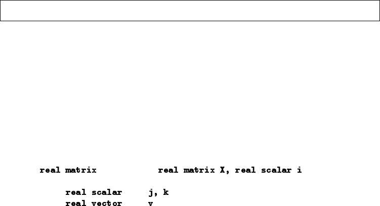
Title
[M-2] declarations — Declarations and types
Syntax Description Remarks and examples Also see
Syntax
declaration1fcnname(declaration2)
{
declaration3
. . .
}
such as
myfunction( )
{
. . .
}
declaration1is one of
function
type function
void function
declaration2is
type argname ,type argname ,. . .
where argname is the name you wish to assign to the argument.
declaration3are lines of the form of either of
type varname ,varname ,. . .
external type varname ,varname ,. . .
type is defined as one of
eltype orgtype such as real vector
eltype such as real
orgtype such as vector
100

[M-2] declarations — Declarations and types 101
eltype and orgtype are each one of
eltype orgtype
transmorphic matrix
numeric vector
real rowvector
complex colvector
string scalar
pointer
If eltype is not specified, transmorphic is assumed. If orgtype is not specified, matrix is assumed.
Description
The type and the use of declarations are explained. Also discussed is the calling convention (functions
are called by address, not by value, and so may change the caller’s arguments), and the use of external
globals.
Mata also has structures—the eltype is struct name—but these are not discussed here. For a
discussion of structures, see [M-2]struct.
Mata also has classes—the eltype is class name—but these are not discussed here. For a discussion
of classes, see [M-2]class.
Declarations are optional but, for careful work, their use is recommended.
Remarks and examples
Remarks are presented under the following headings:
The purpose of declarations
Types, element types, and organizational types
Implicit declarations
Element types
Organizational types
Function declarations
Argument declarations
The by-address calling convention
Variable declarations
Linking to external globals
The purpose of declarations
Declarations occur in three places: in front of function definitions, inside the parentheses defining
the function’s arguments, and at the top of the body of the function, defining private variables the
function will use. For instance, consider the function
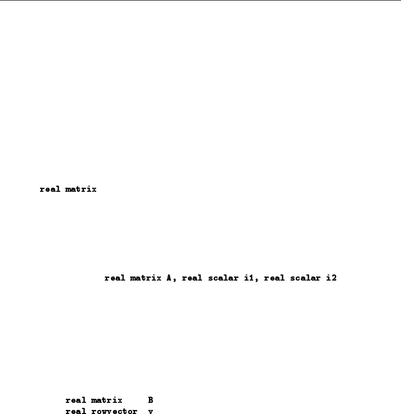
102 [M-2] declarations — Declarations and types
real matrix swaprows(real matrix A, real scalar i1, real scalar i2)
{
real matrix B
real rowvector v
B=A
v = B[i1, .]
B[i1, .] = B[i2, .]
B[i2, .] = v
return(B)
}
This function returns a copy of matrix Awith rows i1 and i2 swapped.
There are three sets of declarations in the above function. First, there is a declaration in front of the
function name:
swaprows(. . . )
{
. . .
}
That declaration states that this function will return a real matrix.
The second set of declarations occur inside the parentheses:
. . . swaprows( )
{
. . .
}
Those declarations state that this function expects to receive three arguments, which we chose to call
A,i1, and i2, and which we expect to be a real matrix, a real scalar, and a real scalar, respectively.
The third set of declarations occur at the top of the body of the function:
. . . swaprows(. . . )
{
. . .
}
Those declarations state that we will use variables Band vinside our function and that, as a matter
of fact, Bwill be a real matrix and va real row vector.
We could have omitted all those declarations. Our function could have read
function swaprows(A, i1, i2)
{
B=A
v = B[i1, .]
B[i1, .] = B[i2, .]
B[i2, .] = v
return(B)
}

[M-2] declarations — Declarations and types 103
and it would have worked just fine. So why include the declarations?
1. By including the outside declaration, we announced to other programs what to expect. They
can depend on swaprows() returning a real matrix because, when swaprows() is done,
Mata will verify that the function really is returning a real matrix and, if it is not, abort
execution.
Without the outside declaration, anything goes. Our function could return a real scalar in
one case, a complex row vector in another, and nothing at all in yet another case.
Including the outside declaration makes debugging easier.
2. By including the argument declaration, we announced to other programmers what they are
expected to pass to our function. We have made it easier to understand our function.
We have also told Mata what to expect and, if some other program attempts to use our
function incorrectly, Mata will stop execution.
Just as in (1), we have made debugging easier.
3. By including the inside declaration, we have told Mata what variables we will need and how
we will be using them. Mata can do two things with that information: first, it can make
sure that we are using the variables correctly (making debugging easier again), and second,
Mata can produce more efficient code (making our function run faster).
Interactively, we admit that we sometimes define functions without declarations. For more careful
work, however, we include them.
Types, element types, and organizational types
When you use Mata interactively, you just willy-nilly create new variables:
: n = 2
: A = (1,2 \ 3,4)
: z = (sqrt(-4+0i), sqrt(4))
When you create a variable, you may not think about the type, but Mata does. nabove is, to Mata,
a real scalar. Ais a real matrix. zis a complex row vector.
Mata thinks of the type of a variable as having two parts:
1. the type of the elements the variable contains (such as real or complex) and
2. how those elements are organized (such as a row vector or a matrix).
We call those two types the eltype—element type—and orgtype—organizational type. The eltypes and
orgtypes are
eltype orgtype
transmorphic matrix
numeric vector
real rowvector
complex colvector
string scalar
pointer
You may choose one of each and so describe all the types Mata understands.

104 [M-2] declarations — Declarations and types
Implicit declarations
When you do not declare an object, Mata behaves as if you declared it to be transmorphic matrix:
1. transmorphic means that the matrix can be real,complex,string, or pointer.
2. matrix means that the organization is to be r×c,r≥0 and c≥0.
At one point in your function, a transmorphic matrix might be a real scalar (real being a
special case of transmorphic and scalar being a special case of a matrix when r=c=1), and
at another point, it might be a string colvector (string being a special case of transmorphic,
and colvector being a special case of a matrix when c=1).
Consider our swaprows() function without declarations,
function swaprows(A, i1, i2)
{
B=A
v = B[i1, .]
B[i1, .] = B[i2, .]
B[i2, .] = v
return(B)
}
The result of compiling this function is just as if the function read
transmorphic matrix swaprows(transmorphic matrix A,
transmorphic matrix i1,
transmorphic matrix i2)
{
transmorphic matrix B
transmorphic matrix v
B=A
v = B[i1, .]
B[i1, .] = B[i2, .]
B[i2, .] = v
return(B)
}
When we declare a variable, we put restrictions on it.
Element types
There are six eltypes, or element types:
1. transmorphic, which means real,complex,string, or pointer.
2. numeric, which means real or complex.
3. real, which means that the elements are real numbers, such as 1, 3, −50, and 3.14159.
4. complex, which means that each element is a pair of numbers, which are given the
interpretation a+bi.complex is a storage type; the number stored in a complex might
be real, such as 2 +0i.

[M-2] declarations — Declarations and types 105
5. string, which means the elements are strings of text. Each element may contain up to
2,147,483,647 characters and strings may (need not) contain binary 0; that is, strings may
be binary strings or text strings. Mata strings are similar to the strL type in Stata in that
they can be very long and may contain binary 0.
6. pointer means the elements are pointers to (addresses of) other Mata matrices, vectors,
scalars, or even functions; see [M-2]pointers.
Organizational types
There are five orgtypes, or organizational types:
1. matrix, which means r×c,r≥0 and c≥0.
2. vector, which means 1 ×nor n×1, n≥0.
3. rowvector, which means 1 ×n,n≥0.
4. colvector, which means n×1, n≥0.
5. scalar, which means 1 ×1.
Sharp-eyed readers will note that vectors and matrices can have zero rows or columns! See [M-2]void
for more information.
Function declarations
Function declarations are the declarations that appear in front of the function name, such as
swaprows(. . . )
{
. . .
}
The syntax for what may appear there is
function
type function
void function
Something must appear in front of the name, and if you do not want to declare the type (which makes
the type transmorphic matrix), you just put the word function:
swaprows(. . . )
{
. . .
}
You may also declare the type and include the word function if you wish,
swaprows(. . . )
{
. . .
}
but most programmers omit the word function; it makes no difference.

106 [M-2] declarations — Declarations and types
In addition to all the usual types, void is a type allowed only with functions—it states that the
function returns nothing:
_swaprows(real matrix A, real scalar i1, real scalar i2)
{
real rowvector v
v = A[i1, .]
A[i1, .] = A[i2, .]
A[i2, .] = v
}
The function above returns nothing; it instead modifies the matrix it is passed. That might be useful
to save memory, especially if every use of the original swaprows() was going to be
A = swaprows(A, i1, i2)
In any case, we named this new function swaprows() (note the underscore), to flag the user that
there is something odd and deserving caution concerning the use of this function.
void, that is to say, returning nothing, is also considered a special case of a transmorphic matrix
because Mata secretly returns a 0 ×0 real matrix, which the caller just discards.
Argument declarations
Argument declarations are the declarations that appear inside the parentheses, such as
. . . swaprows( )
{
. . .
}
The syntax for what may appear there is
type argname ,type argname ,. . .
The names are required—they specify how we will refer to the argument—and the types are optional.
Omit the type and transmorphic matrix is assumed. Specify the type, and it will be checked
when your function is called. If the caller attempts to use your function incorrectly, Mata will stop
the execution and complain.
The by-address calling convention
Arguments are passed to functions by address, not by value. If you change the value of an argument,
you will change the caller’s argument. That is what made swaprows() (above) work. The caller
passed us Aand we changed it. And that is why in the original version of swaprows(), the first line
read
B=A
we did our work on B, and returned B. We did not want to modify the caller’s original matrix.

[M-2] declarations — Declarations and types 107
You do not ordinarily have to make copies of the caller’s arguments, but you do have to be careful
if you do not want to change the argument. That is why in all the official functions (with the single
exception of st view()—see [M-5]st view( )), if a function changes the caller’s argument, the
function’s name starts with an underscore. The reverse logic does not hold: some functions start with
an underscore and do not change the caller’s argument. The underscore signifies caution, and you
need to read the function’s documentation to find out what it is you need to be cautious about.
Variable declarations
The variable declarations are the declarations that appear at the top of the body of a function:
. . . swaprows(. . . )
{
. . .
}
These declarations are optional. If you omit them, Mata will observe that you are using Band vin
your code, and then Mata will compile your code just as if you had declared the variables to be
transmorphic matrix, meaning that the resulting compiled code might be a little more inefficient
than it could be, but that is all.
The variable declarations are optional as long as you have not mata set matastrict on; see
[M-3]mata set. Some programmers believe so strongly that variables really ought to be declared that
Mata provides a provision to issue an error when they forget.
In any case, these declarations—explicit or implicit—define the variables we will use. The variables
we use in our function are private—it does not matter if there are other variables named Band v
floating around somewhere. Private variables are created when a function is invoked and destroyed
when the function ends. The variables are private but, as explained above, if we pass our variables
to another function, that function may change their values. Most functions do not.
The syntax for declaring variables is
type varname ,varname ,. . .
external type varname ,varname ,. . .
real matrix B and real rowvector v match the first syntax.
Linking to external globals
The second syntax has to do with linking to global variables. When you use Mata interactively and
type
: n = 2
you create a variable named n. That variable is global. When you code inside a function
. . . myfunction(. . . )
{
. . .
}

108 [M-2] declarations — Declarations and types
The nvariable your function will use is the global variable named n. If your function were to examine
the value of nright now, it would discover that it contained 2.
If the variable does not already exist, the statement external n will create it. Pretend that we had
not previously defined n. If myfunction() were to examine the contents of n, it would discover
that nis a 0 ×0 matrix. That is because we coded
external n
and Mata behaved as if we had coded
external transmorphic matrix n
Let’s modify myfunction() to read:
. . . myfunction(. . . )
{
. . .
}
Let’s consider the possibilities:
1. ndoes not exist. Here external real scalar n will create n—as a real scalar, of
course—and set its value to missing.
If nhad been declared a rowvector, a 1 ×0 vector would have been created.
If nhad been declared a colvector, a 0 ×1 vector would have been created.
If nhad been declared a vector, a 0 ×1 vector would have been created. Mata could just
as well have created a 1 ×0 vector, but it creates a 0 ×1.
If nhad been declared a matrix, a 0 ×0 matrix would have been created.
2. nexists, and it is a real scalar. Our function executes, using the global n.
3. nexists, and it is a real 1×1rowvector,colvector, or matrix. The important thing
is that it is 1 ×1; our function executes, using the global n.
4. nexists, but it is complex or string or pointer, or it is real but not 1 ×1. Mata
issues an error message and aborts execution of our function.
Complicated systems of programs sometimes find it convenient to communicate via globals. Because
globals are globals, we recommend that you give your globals long names. A good approach is to
put the name of your system as a prefix:
. . . myfunction(. . . )
{
. . .
}
For another approach to globals, see [M-5]findexternal( ) and [M-5]valofexternal( ).


Title
[M-2] do — do . . . while (exp)
Syntax Description Remarks and examples Also see
Syntax
do stmt while (exp)
do {
stmts
} while (exp)
where exp must evaluate to a real scalar.
Description
do executes stmt or stmts one or more times, until exp is zero.
Remarks and examples
One common use of do is to loop until convergence:
do {
lasta = a
a = get_new_a(lasta)
} while (mreldif(a, lasta)>1e-10)
The loop is executed at least once, and the conditioning expression is not executed until the loop’s
body has been executed.
Also see
[M-2]for — for (exp1; exp2; exp3) stmt
[M-2]while — while (exp) stmt
[M-2]break — Break out of for, while, or do loop
[M-2]continue — Continue with next iteration of for, while, or do loop
[M-2]intro — Language definition
110

Title
[M-2] errors — Error codes
Description Remarks and examples Also see
Description
When an error occurs, Mata presents a number as well as text describing the problem. The codes are
presented below.
Also the error codes can be used as an argument with error(), see [M-5]error( ).
Mata’s error codes are a special case of Stata’s return codes. In particular, they are the return codes
in the range 3000–3999. In addition to the 3000-level codes, it is possible for Mata functions to
generate any Stata error message and return code.
Remarks and examples
Error messages in Mata break into two classes: errors that occur when the function is compiled (code
3000) and errors that occur when the function is executed (codes 3001–3999).
Compile-time error messages look like this:
: 2,,3
invalid expression
r(3000);
: "this" + "that
mismatched quotes
r(3000);
The text of the message varies according to the error made, but the error code is always 3000.
Run-time errors look like this:
: myfunction(2,3)
solve(): 3200 conformability error
mysub(): - function returned error
myfunction(): - function returned error
<istmt>: - function returned error
r(3200);
The output is called a traceback log. Read from bottom to top, it says that what we typed (the
<istmt>) called myfunction(), which called mysub(), which called solve() and, at that point,
things went wrong. The error is possibly in solve(), but because solve() is a library function, it
is more likely that the error is in how mysub() called solve(). Moreover, the error is seldom in
the program listed at the top of the traceback log because the log lists the identity of the program
that detected the error. Say solve() did have an error. Then the traceback log would probably have
read something like
*: 3200 conformability error
solve(): - function returned error
mysub(): - function returned error
myfunction(): - function returned error
<istmt>: - function returned error
111

112 [M-2] errors — Error codes
The above log says the problem was detected by *(the multiplication operator), and at that point,
solve() would be suspect, because one must ask, why did solve() use the multiplication operator
incorrectly?
In any case, let’s assume that the problem is not with solve(). Then you would guess the problem lies
with mysub(). If you have used mysub() in many previous programs without problems, however, you
might now shift your suspicion to myfunction(). If myfunction() is always trustworthy, perhaps
you should not have typed myfunction(2,3). That is, perhaps you are using myfunction()
incorrectly.
The error codes
3000. (message varies)
There is an error in what you have typed. Mata cannot interpret what you mean.
3001. incorrect number of arguments
The function expected, say, three arguments and received two, or five. Or the function allows
between three and five arguments, but you supplied too many or too few. Fix the calling
program.
3002. identical arguments not allowed
You have called a function specifying the same variable more than once. Usually this would
not be a problem, but here, it is, usually because the supplied arguments are matrices that
the function wishes to overwrite with different results. For instance, say function f(A,B,
C)examines matrix Aand returns a calculation based on Ain Band C. The function might
well complain that you specified the same matrix for Band C.
3010. attempt to dereference NULL pointer
The program made reference to *s, and scontains NULL; see [M-2]pointers.
3011. invalid lval
In an assignment, what appears on the left-hand side of the equals is not something to which
a value can be assigned; see [M-2]op assignment.
3012. undefined operation on pointer
You have, for instance, attempted to add two pointers; see [M-2]pointers.
3020. class child/parent compiled at different times
One class is being used to extend another class, and the parent has been updated since the
class was compiled.
3021. class compiled at different times
A function using a predefined class has not been recompiled since the class has last been
changed.
3022. function not supported on this platform
You have tried to use a function that is defined for some operating system or flavor supported
by Stata but not for the one you are currently using. For example, you may have tried to
use a Mac-only function in Stata for Windows.
3101. matrix found where function required
A particular argument to a function is required to be a function, and a matrix was found
instead.

[M-2] errors — Error codes 113
3102. function found where matrix required
A particular argument to a function is required to be a matrix, vector, or scalar, and a
function was found instead.
3103. view found where array required
In general, view matrices can be used wherever a matrix is required, but there are a few
exceptions, both in low-level routines and in routines that wish to write results back to the
argument. Here a view is not acceptable. If Vis the view variable, simply code X=Vand
then pass Xin its stead. See [M-5]st view( ).
3104. array found where view required
A function argument was specified with a matrix that was not a view, and a view was
required. See [M-5]st view( ).
3200. conformability error
A matrix, vector, or scalar has the wrong number of rows and/or columns for what is
required. Adding a 2 ×3 matrix to a 1 ×4 would result in this error.
3201. vector required
An argument is required to be r×1 or 1 ×c, and a matrix was found instead.
3202. rowvector required
An argument is required to be 1 ×cand it is not.
3203. colvector required
An argument is required to be r×1 and it is not.
3204. matrix found where scalar required
An argument is required to be 1 ×1 and it is not.
3205. square matrix required
An argument is required to be n×nand it is not.
3206. invalid use of view containing op.vars
Factor variables have been used in a view, and the view is now being used in a context that
does not support the use of factor variables.
3250. type mismatch
The eltype of an argument does not match what is required. For instance, perhaps a real
was expected and a string was received. See eltype in [M-6]Glossary.
3251. nonnumeric found where numeric required
An argument was expected to be real or complex and it is not.
3252. noncomplex found where complex required
An argument was expected to be complex and it is not.
3253. nonreal found where real required
An argument was expected to be real and it is not.
3254. nonstring found where string required
An argument was expected to be string and it is not.
3255. real or string required
An argument was expected to be real or string and it is not.

114 [M-2] errors — Error codes
3256. numeric or string required
An argument was expected to be real, complex, or string and it is not.
3257. nonpointer found where pointer required
An argument was expected to be a pointer and it is not.
3258. nonvoid found where void required
An argument was expected to be void and it is not.
3259. nonstruct found where struct required
A variable that is not a structure was passed to a function that expected the variable to be
a structure.
3260. nonclass found where class required
A variable that is not a class was passed to a function that expected the variable to be a
class.
3261. non class/struct found where class/struct required
A variable that is not a class or a structure was passed to a function that expected the variable
to be a class or a structure.
3300. argument out of range
The eltype and orgtype of the argument are correct, but the argument contains an invalid
value, such as if you had asked for the 20th row of a 4 ×5 matrix. See eltype and orgtype
in [M-6]Glossary.
3301. subscript invalid
The subscript is out of range (refers to a row or column that does not exist) or contains the
wrong number of elements. See [M-2]subscripts.
3302. invalid %fmt
The %fmt for formatting data is invalid. See [M-5]printf( ) and see [U] 12.5 Formats:
Controlling how data are displayed.
3303. invalid permutation vector
The vector specified does not meet the requirements of a permutation vector, namely, that an
n-element vector contain a permutation of the integers 1 through n. See [M-1]permutation.
3304. struct nested too deeply
Structures may contain structures that contain structures, and so on, but only to a depth of
500.
3305. class nested too deeply
Classes may contain classes that contain classes, and so on, but only to a depth of 500.
3351. argument has missing values
In general, Mata is tolerant of missing values, but there are exceptions. This function does
not allow the matrix, vector, or scalar to have missing values.
3352. singular matrix
The matrix is singular and the requested result cannot be carried out. If singular matrices
are a possibility, then you are probably using the wrong function.
3353. matrix not positive definite
The matrix is non–positive definite and the requested results cannot be computed. If non–
positive-definite matrices are a possibility, then you are probably using the wrong function.

[M-2] errors — Error codes 115
3360. failure to converge
The function that issued this message used an algorithm that the function expected would
converge but did not, probably because the input matrix was extreme in some way.
3492. resulting string too long
A string that the function was attempting to produce became too long. Because the maximum
length of strings in Mata is 2,147,483,647 characters, it is unlikely that Mata imposed the
limit. Review the documentation on the function for the source of the limit that was imposed
(for example, perhaps a string was being produced for use by Stata). In any case, this error
does not arise because of an out-of-memory situation. It arises because some limit was
imposed.
3498. (message varies)
An error specific to this function arose. The text of the message should describe the problem.
3499. not found
The specified variable or function could not be found. For a function, it was not already
loaded, it is not in the libraries, and there is no .mo file with its name.
3500. invalid Stata variable name
A variable name—which name is contained in a Mata string variable—is not appropriate
for use with Stata.
3598. Stata returned error
You are using a Stata interface function and have asked Stata to perform a task. Stata could
not or refused.
3601. invalid file handle
The number specified does not correspond to an open file handle; see [M-5]fopen( ).
3602. invalid filename
The filename specified is invalid.
3603. invalid file mode
The file mode (whether read, write, read-write, etc.) specified is invalid; see [M-5]fopen( ).
3611. too many open files
The maximum number of files that may be open simultaneously is 50, although your operating
system may not allow that many.
3612. file too large for 32-bit Stata
You are running 32-bit Stata on a 64-bit computer, and the file you wish to process is larger
than 4 gigabytes.
3621. attempt to write read-only file
The file was opened read-only and an attempt was made to write into it.
3622. attempt to read write-only file
The file was opened write-only and an attempt was made to read it.
3623. attempt to seek append-only file
The file was opened append-only and then an attempt was made to seek into the file; see
[M-5]fopen( ).

116 [M-2] errors — Error codes
3698. file seek error
An attempt was made to seek to an invalid part of the file, or the seek failed for other
reasons; see [M-5]fopen( ).
3900. out of memory
Mata is out of memory; the operating system refused to supply what Mata requested. There
is no Mata or Stata setting that affects this, and so nothing in Mata or Stata to reset in order
to get more memory. You must take up the problem with your operating system.
3901. macro memory in use
This error message should not occur; please notify StataCorp if it does.
3930. error in LAPACK routine
The linear-algebra LAPACK routines—see [M-1]LAPACK—generated an error that Mata did
not expect. Please notify StataCorp if you should receive this error.
3995. unallocated function
This error message should not occur; please notify StataCorp if it does.
3996. built-in unallocated
This error message should not occur; please notify StataCorp if it does.
3997. unimplemented opcode
This error message should not occur; please notify StataCorp if it does.
3998. stack overflow
Your program nested too deeply. For instance, imagine calculating the factorial of nby
recursively calling yourself and then requesting the factorial of 1e+100. Functions that call
themselves in an infinite loop inevitably cause this error.
3999. system assertion false
Something unexpected happened in the internal Mata code. Please contact Technical Services
and report the problem. You do not need to exit Stata or Mata. Mata stopped doing what
was leading to a problem.
Also see
[M-5]error( ) — Issue error message
[M-2]intro — Language definition

Title
[M-2] exp — Expressions
Syntax Description Remarks and examples Reference Also see
Syntax
exp
Description
exp is used in syntax diagrams to mean “any valid expression may appear here”. Expressions can
range from being simple constants
2
"this"
3+2i
to being names of variables
A
beta
varwithverylongname
to being a full-fledged scalar, string, or matrix expression:
sqrt(2)/2
substr(userinput, 15, strlen(otherstr))
conj(X)’X
Remarks and examples
Remarks are presented under the following headings:
What’s an expression
Assignment suppresses display, as does (void)
The pieces of an expression
Numeric literals
String literals
Variable names
Operators
Functions
What’s an expression
Everybody knows what an expression is: expressions are things like 2+3 and invsym(X’X)*X’y.
Simpler things are also expressions, such as numeric constants
2is an expression
117

118 [M-2] exp — Expressions
and string literals
"hi there" is an expression
and function calls:
sqrt(2) is an expression
Even when functions do not return anything (the function is void), the code that causes the function to
run is an expression. For instance, the function swap() (see [M-5]swap( )) interchanges the contents
of its arguments and returns nothing. Even so,
swap(A, B) is an expression
Assignment suppresses display, as does (void)
The equal sign assigns the result of an expression to a variable. For instance,
a=2+3
assigns 5 to a. When the result of an expression is not assigned to a variable, the result is displayed at
the terminal. This is true of expressions entered interactively and of expressions coded in programs.
For instance, given the program
function example(a, b)
{
"the answer is"
a+b
}
executing example() produces
: example(2, 3)
the answer is
5
The fact that 5 appeared is easy enough to understand; we coded the expression a+b without assigning
it to another variable. The fact that “the answer is” also appeared may surprise you. Nevertheless,
we coded "the answer is" in our program, and that is an example of an expression, and because
we did not assign the expression to a variable, it was displayed.
In programming situations, there will be times when you want to execute a function—call it setup()—
but do not care what the function returns, even though the function itself is not void (that is, it returns
something). If you code
function example(. . .)
{
. . .
setup(. . .)
. . .
}
the result will be to display what setup() returns. You have two alternatives. You could assign the
result of setup to a variable even though you will subsequently not use the variable

[M-2] exp — Expressions 119
function example(. . .)
{
. . .
result = setup(. . .)
. . .
}
or you could cast the result of the function to be void:
function example(. . .)
{
. . .
(void) setup(. . .)
. . .
}
Placing (void) in front of an expression prevents the result from being displayed.
The pieces of an expression
Expressions comprise
numeric literals
string literals
variable names
operators
functions
Numeric literals
Numeric literals are just numbers
2
3.14159
-7.2
5i
1.213e+32
1.213E+32
1.921fb54442d18X+001
1.921fb54442d18x+001
.
.a
.b
but you can suffix an ionto the end to mean imaginary, such as 5i above. To create complex
numbers, you combine real and imaginary numbers using the +operator, as in 2+5i. In any case, you
can put the ion the end of any literal, so 1.213e+32i is valid, as is 1.921fb54442d18X+001i.
1.921fb54442d18X+001i is a formidable-looking beast, with or without the i.
1.921fb54442d18X+001 is a way of writing floating-point numbers in binary; it is described in
[U] 12.5 Formats: Controlling how data are displayed. Most people never use it.
Also, numeric literals include Stata’s missing values, .,.a,.b,. . . ,.z.

120 [M-2] exp — Expressions
Complex variables may contain missing just as real variables may, but they get only one: .a+.bi is
not allowed. A complex variable contains a valid complex value, or it contains .,.a,.b,. . . ,.z.
String literals
String literals are enclosed in double quotes or in compound double quotes:
"the answer is"
"a string"
‘"also a string"’
‘"The "factor" of a matrix"’
""
‘""’
Strings in Mata contain between 0 and 2,147,483,647 characters. "" or ‘""’ is how one writes the
0-length string.
Any ASCII character may appear in the string, but no provision is provided for typing the unprintable
ASCII characters into the string literal. Instead, you use the char() function; see [M-5]ascii( ). For
instance, char(13) is carriage return, so the expression
"my string" + char(13)
produces “my string” followed by a carriage return.
No character is given a special interpretation. In particular, backslash (\) is given no special meaning
by Mata. The string literal "my string\n" is just that: the characters “my string” followed by a
backslash followed by an “n”. Some functions, such as printf() (see [M-5]printf( )), give a special
meaning to the two-character sequence \n, but that special interpretation is a property of the function,
not Mata, and is noted in the function’s documentation.
Strings are not zero (null) terminated in Mata. Mata knows that the string "hello" is of length 5,
but it does not achieve that knowledge by padding a binary 0 as the string’s fifth character. Thus
strings may be used to hold binary information.
Although Mata gives no special interpretation to binary 0, some Mata functions do. For instance,
strmatch(s,pattern)returns 1 if smatches pattern and 0 otherwise; see [M-5]strmatch( ). For
this function, both strings are considered to end at the point they contain a binary 0, if they contain a
binary 0. Most strings do not, and then the function considers the entire string. In any case, if there
is special treatment of binary 0, that is on a function-by-function basis, and a note of that is made
in the function’s documentation.
Variable names
Variable names are just that. Names are case sensitive and no abbreviations are allowed:
X
x
MyVar
VeryLongVariableNameForUseInMata
MyVariable
The maximum length of a variable name is 32 characters.

[M-2] exp — Expressions 121
Operators
Operators, listed by precedence, low to high
Operator Operator name Documentation
a=bassignment [M-2]op assignment
a?b:cconditional [M-2]op conditional
a\bcolumn join [M-2]op join
a:: bcolumn to [M-2]op range
a,brow join [M-2]op join
a.. brow to [M-2]op range
a:| be.w. or [M-2]op colon
a|bor [M-2]op logical
a:& be.w. and [M-2]op colon
a&band [M-2]op logical
a:== be.w. equal [M-2]op colon
a== bequal [M-2]op logical
a:>= be.w. greater than or equal [M-2]op colon
a>= bgreater than or equal [M-2]op logical
a:<= be.w. less than or equal [M-2]op colon
a<= bless than or equal [M-2]op logical
a:< be.w. less than [M-2]op colon
a<bless than [M-2]op logical
a:> be.w. greater than [M-2]op colon
a>bgreater than [M-2]op logical
a:!= be.w. not equal [M-2]op colon
a!= bnot equal [M-2]op logical
a:+ be.w. addition [M-2]op colon
a+baddition [M-2]op arith
a:- be.w. subtraction [M-2]op colon
a-bsubtraction [M-2]op arith
a:* be.w. multiplication [M-2]op colon
a*bmultiplication [M-2]op arith
a#bKronecker [M-2]op kronecker
a:/ be.w. division [M-2]op colon
a/bdivision [M-2]op arith
-anegation [M-2]op arith
a:^ be.w. power [M-2]op colon
a^bpower [M-2]op arith
a’transposition [M-2]op transpose
*acontents of [M-2]pointers
&aaddress of [M-2]pointers
!anot [M-2]op logical
a[exp]subscript [M-2]subscripts
a[|exp|] range subscript [M-2]subscripts
a++ increment [M-2]op increment
a-- decrement [M-2]op increment
++aincrement [M-2]op increment
--adecrement [M-2]op increment
(e.w. = elementwise)


Title
[M-2] for — for (exp1; exp2; exp3) stmt
Syntax Description Remarks and examples Also see
Syntax
for (exp1;exp2;exp3)stmt
for (exp1;exp2;exp3) {
stmts
}
where exp1and exp3are optional, and exp2must evaluate to a real scalar.
Description
for is equivalent to
exp1
while (exp2) {
stmt(s)
exp3
}
stmt(s) is executed zero or more times. The loop continues as long as exp2 is not equal to zero.
Remarks and examples
To understand for, enter the following program
function example(n)
{
for (i=1; i<=n; i++) {
printf("i=%g\n", i)
}
printf("done\n")
}
and run example(3),example(2),example(1),example(0), and example(-1).
Common uses of for include
for (i=1; i<=rows(A); i++) {
for (j=1; j<=cols(A); j++) {
. . .
}
}
123


Title
[M-2] ftof — Passing functions to functions
Syntax Description Remarks and examples Also see
Syntax
example(. . ., &somefunction(), . . . )
where example() is coded
function example(. . .,f,. . . )
{
. . .
(*f)(. . .)
. . .
}
Description
Functions can receive other functions as arguments.
Below is described (1) how to call a function that receives a function as an argument and (2) how
to write a function that receives a function as an argument.
Remarks and examples
Remarks are presented under the following headings:
Passing functions to functions
Writing functions that receive functions, the simplified convention
Passing built-in functions
Passing functions to functions
Someone has written a program that receives a function as an argument. We will imagine that function
is
real scalar fderiv(function(), x)
and that fderiv() numerically evaluates the derivative of function() at x. The documentation for
fderiv() tells you to write a function that takes one argument and returns the evaluation of the
function at that argument, such as
real scalar expratio(real scalar x)
{
return(exp(x)/exp(-x))
}
125

126 [M-2] ftof — Passing functions to functions
To call fderiv() and have it evaluate the derivative of expratio() at 3, you code
fderiv(&expratio(), 3)
To pass a function to a function, you code &in front of the function’s name and () after. Coding
&expratio() passes the address of the function expratio() to fderiv().
Writing functions that receive functions, the simplified convention
To receive a function, you include a variable among the program arguments to receive the function—we
will use f—and you then code (*f)(. . . )to call the passed function. The code for fderiv() might
read
function fderiv(f, x)
{
return( ((*f)(x+1e-6) - (*f)(x)) / 1e-6 )
}
or, if you prefer to be explicit about your declarations,
real scalar fderiv(pointer scalar f, real scalar x)
{
return( ((*f)(x+1e-6) - (*f)(x)) / 1e-6 )
}
or, if you prefer to be even more explicit:
real scalar fderiv(pointer(real scalar function) scalar f,
real scalar x)
{
return( ((*f)(x+1e-6) - (*f)(x)) / 1e-6 )
}
In any case, using pointers, you type (*f)(. . .)to execute the function passed. See [M-2]pointers
for more information.
Aside: the function fderiv() would work but, because of the formula it uses, would return very
inaccurate results.
Passing built-in functions
You cannot pass built-in functions to other functions. For instance, [M-5]exp( ) is built in, which is
revealed by [M-3]mata which:
: mata which exp()
exp(): built-in
Not all official functions are built in. Many are implemented in Mata as library functions, but exp()
is built in and coding &exp() will result in an error. If you wanted to pass exp() to a function,
create your own version of it
: function myexp(x) return(exp(x))
and then pass &myexp().


Title
[M-2] goto — goto label
Syntax Description Remarks and examples Reference Also see
Syntax
label:. . .
. . .
goto label
where label:may occur before or after the goto.
Description
goto label causes control to pass to the statement following label:.label may be any name up to
eight characters long.
Remarks and examples
These days, good style is to avoid using goto.
goto is useful when translating a FORTRAN program, such as
A = 4.0e0/3.0e0
10 B = A - 1.0e0
C=B+B+B
EPS = DABS(C - 1.0e0)
if (EPS.EQ.0.0e0) GOTO 10
The Mata translation is
a = 4/3
s10: b = a - 1
c=b+b+b
eps = abs(c-1)
if (eps==0) goto s10
although
a = 4/3
do {
b=a-1
c=b+b+b
eps = abs(c - 1)
} while (eps==0)
is more readable.
128

[M-2] goto — goto label 129
Reference
Gould, W. W. 2005. Mata Matters: Translating Fortran.Stata Journal 5: 421–441.
Also see
[M-2]do — do . . . while (exp)
[M-2]for — for (exp1; exp2; exp3) stmt
[M-2]while — while (exp) stmt
[M-2]break — Break out of for, while, or do loop
[M-2]continue — Continue with next iteration of for, while, or do loop
[M-2]intro — Language definition

Title
[M-2] if — if (exp) . . . else . . .
Syntax Description Remarks and examples Also see
Syntax
if (exp)stmt1
if (exp)stmt1
else stmt2
if (exp) {
stmts1
}
else {
stmts2
}
if (exp1). . .
else if (exp2). . .
else if (exp3). . .
. . .
else . . .
where exp,exp1,exp2,exp3,. . . must evaluate to real scalars.
Description
if evaluates the expression, and if it is true (evaluates to a nonzero number), if executes the statement
or statement block that immediately follows it; otherwise, if skips the statement or block.
if . . . else evaluates the expression, and if it is true (evaluates to a nonzero number), if executes
the statement or statement block that immediately follows it and skips the statement or statement
block following the else; otherwise, it skips the statement or statement block immediately following
it and executes the statement or statement block following the else.
130

[M-2] if — if (exp) . . . else . . . 131
Remarks and examples
if followed by multiple elses is interpreted as being nested, that is,
if (exp1). . .
else if (exp2). . .
else if (exp3). . .
. . .
else . . .
is equivalent to
if (exp1). . .
else {
if (exp2). . .
else {
if (exp3). . .
else {
. . .
}
}
}
Also see
[M-2]intro — Language definition

Title
[M-2] op arith — Arithmetic operators
Syntax Description Remarks and examples Conformability
Diagnostics Also see
Syntax
a+baddition
a-bsubtraction
a*bmultiplication
a/bdivision
a^bpower
-anegation
where aand bmay be numeric scalars, vectors, or matrices.
Description
The above operators perform basic arithmetic.
Remarks and examples
Also see [M-2]op colon for the :+,:-,:*, and :/ operators. Colon operators have relaxed
conformability restrictions.
The *and :* multiplication operators can also perform string duplication—3*"a" = "aaa"—see
[M-5]strdup( ).
Conformability
a+b,a-b:a:r×c
b:r×c
result:r×c
a*b:a:k×n k ×n1×1
b:n×m1×1n×m
result:k×m k ×n n ×m
a/b:a:r×c
b: 1 ×1
result:r×c
a^b:a: 1 ×1
b: 1 ×1
result: 1 ×1
132

[M-2] op arith — Arithmetic operators 133
-a:a:r×c
result:r×c
Diagnostics
All operators return missing when arguments are missing.
a*bwith a:k×0 and b: 0 ×mreturns a k×mmatrix of zeros.
a/breturns missing when b==0 or when a/bwould result in overflow.
a^breturns a real when both aand bare real; thus, (-4)^.5 evaluates to missing, whereas
(-4+0i)^.5 evaluates to 2i.
a^breturns missing on overflow.
Also see
[M-2]exp — Expressions
[M-2]intro — Language definition

Title
[M-2] op assignment — Assignment operator
Syntax Description Remarks and examples Conformability
Diagnostics Also see
Syntax
lval =exp
where exp is any valid expression and where lval is
name
name[exp]
name[exp,exp]
name[|exp|]
In pointer use (advanced), name may be
*lval
*(lval)
*(lval[exp])
*(lval[exp,exp])
*(lval[|exp|])
in addition to being a variable name.
Description
=assigns the evaluation of exp to lval.
Do not confuse the =assignment operator with the == equality operator. Coding
x=y
assigns the value of yto x. Coding
if (x==y) . . . (note doubled equal signs)
performs the action if the value of xis equal to the value of y. See [M-2]op logical for a description
of the == equality operator.
If the result of an expression is not assigned to a variable, then the result is displayed at the terminal;
see [M-2]exp.
Remarks and examples
Remarks are presented under the following headings:
Assignment suppresses display
The equal-assignment operator
lvals, what appears on the left-hand side
Row, column, and element lvals
Pointer lvals
134

[M-2] op assignment — Assignment operator 135
Assignment suppresses display
When you interactively enter an expression or code an expression in a program without the equal-
assignment operator, the result of the expression is displayed at the terminal:
: 2 + 3
5
When you assign the expression to a variable, the result is not displayed:
:x=2+3
The equal-assignment operator
Equals is an operator, so in addition to coding
a=2+3
you can code
a=b=2+3
or
y = x / (denominator = sqrt(a+b))
or even
y1 = y2 = x / (denominator = sqrt(sum=a+b))
This last is equivalent to
sum = a + b
denominator = sqrt(sum)
y2 = x / denominator
y1 = y2
Equals binds weakly, so
a=b=2+3
is interpreted as
a=b=(2+3)
and not
a = (b=2) + 3
lvals, what appears on the left-hand side
What appears to the left of the equals is called an lval, short for left-hand-side value. It would make
no sense, for instance, to code
sqrt(4) = 3

136 [M-2] op assignment — Assignment operator
and, as a matter of fact, you are not allowed to code that because sqrt(4) is not an lval:
: sqrt(4) = 3
invalid lval
r(3000);
An lval is anything that can hold values. A scalar can hold values
a=3
x = sqrt(4)
a matrix can hold values
A = (1, 2 \ 3, 4)
B = invsym(C)
a matrix row can hold values
A[1,.] = (7, 8)
a matrix column can hold values
A[.,2] = (9 \ 10)
and finally, a matrix element can hold a value
A[1,2] = 7
lvals are usually one of the above forms. The other forms have to do with pointer variables, which
most programmers never use; they are discussed under Pointer lvals below.
Row, column, and element lvals
When you assign to a row, column, or element of a matrix,
A[1,.] = (7, 8)
A[.,2] = (9 \ 10)
A[1,2] = 7
the row, column, or element must already exist:
: A = (1, 2 \ 3, 4)
: A[3,4] = 4
<istmt>: 3301 subscript invalid
r(3301);
This is usually not an issue because, by the time you are assigning to a row, column, or element, the
matrix has already been created, but in the event you need to create it first, use the J() function; see
[M-5]J( ). The following code fragment creates a 3 ×4 matrix containing the sum of its indices:
A = J(3, 4, .)
for (i=1; i<=3; i++) {
for (j=1; j<=4; j++) A[i,j] = i + j
}

[M-2] op assignment — Assignment operator 137
Pointer lvals
In addition to the standard lvals
A = (1, 2 \ 3, 4)
A[1,.] = (7, 8)
A[.,2] = (9 \ 10)
A[1,2] = 7
pointer lvals are allowed. For instance,
*p = 3
stores 3 in the address pointed to by pointer scalar p.
(*q)[1,2] = 4
stores 4 in the (1,2) element of the address pointed to by pointer scalar q, whereas
*Q[1,2] = 4
stores 4 in the address pointed to by the (1,2) element of pointer matrix Q.
*Q[2,1][1,3] = 5
is equivalent to
*(Q[2,1])[1,3] = 5
and stores 5 in the (1,3) element of the address pointed to by the (2,1) element of pointer matrix Q.
Pointers to pointers, pointers to pointers to pointers, etc., are also allowed. For instance,
**r = 3
stores 3 in the address pointed to by the address pointed to by pointer scalar r, whereas
*((*(Q[1,2]))[2,1])[3,4] = 7
stores 7 in the (3,4) address pointed to by the (2,1) address pointed to by the (1,2) address of pointer
matrix Q.
Conformability
a=b:
input:
b:r×c
output:
a:r×c
Diagnostics
a=baborts with error if there is insufficient memory to store a copy of bin a.


Title
[M-2] op colon — Colon operators
Syntax Description Remarks and examples Conformability
Diagnostics Also see
Syntax
a:+ baddition
a:- bsubtraction
a:* bmultiplication
a:/ bdivision
a:^ bpower
a:== bequality
a:!= binequality
a:> bgreater than
a:>= bgreater than or equal to
a:< bless than
a:<= bless than or equal to
a:& band
a:| bor
Description
Colon operators perform element-by-element operations.
Remarks and examples
Remarks are presented under the following headings:
C-conformability: element by element
Usefulness of colon logical operators
Use parentheses
C-conformability: element by element
The colon operators perform the indicated operation on each pair of elements of aand b. For instance,
c d
f g
h i
:*
j k
l m
n o
=
c∗j d ∗k
f∗l g ∗m
h∗n i ∗o
139

140 [M-2] op colon — Colon operators
Also colon operators have a relaxed definition of conformability:
c
f
g
:*
j k
l m
n o
=
c∗j c ∗k
f∗l f ∗m
g∗n g ∗o
c d
f g
h i
:*
j
l
n
=
c∗j d ∗j
f∗l g ∗l
h∗n i ∗n
[c d ]:*
j k
l m
n o
=
c∗j d ∗k
c∗l d ∗m
c∗n d ∗o
c d
f g
h i
:* [l m ] =
c∗l d ∗m
f∗l g ∗m
h∗l i ∗m
c:*
j k
l m
n o
=
c∗j c ∗k
c∗l c ∗m
c∗n c ∗o
c d
f g
h i
:* j=
c∗j d ∗j
f∗j g ∗j
h∗j i ∗j
The matrices above are said to be c-conformable; the cstands for colon. The matrices have the same
number of rows and columns, or one or the other is a vector with the same number of rows or
columns as the matrix, or one or the other is a scalar.
C-conformability is relaxed, but not everything is allowed. The following is an error:
(c d e):*
f
g
h
Usefulness of colon logical operators
It is worth paying particular attention to the colon logical operators because they can produce pattern
vectors and matrices. Consider the matrix
: x = (5, 0 \ 0, 2 \ 3, 8)
: x
1 2
1 5 0
2 0 2
3 3 8

[M-2] op colon — Colon operators 141
Which elements of xcontain 0?
: x:==0
1 2
1 0 1
2 1 0
3 0 0
How many zeros are there in x?
: sum(x:==0)
2
Use parentheses
Because of their relaxed conformability requirements, colon operators are not associative even when
the underlying operator is. For instance, you expect (a+b)+c== a+(b+c), at least ignoring numerical
roundoff error. Nevertheless, (a:+b):+c== a:+(b:+c) does not necessarily hold. Consider what happens
when
a: 1 ×4
b: 5 ×1
c: 5 ×4
Then (a:+b):+cis an error because a:+bis not c-conformable.
Nevertheless, a:+(b:+c) is not an error and in fact produces a 5 ×4 matrix because b:+cis 5 ×4,
which is c-conformable with a.
Conformability
a:op b:
a:r1×c1
b:r2×c2,aand bc-conformable
result:max(r1,r2)×max(c1,c2)
Diagnostics
The colon operators return missing and abort with error under the same conditions that the underlying
operator returns missing and aborts with error.
Also see
[M-2]exp — Expressions
[M-2]intro — Language definition

Title
[M-2] op conditional — Conditional operator
Syntax Description Remarks and examples Conformability
Diagnostics Also see
Syntax
a?b:c
where amust evaluate to a real scalar, and band cmay be of any type whatsoever.
Description
The conditional operator returns bif ais true (ais not equal to 0) and cotherwise.
Remarks and examples
Conditional operators
dof = (k==0 ? n-1 : n-k)
are more compact than the if–else alternative
if (k==0) dof = n-1
else dof = n-k
and they can be used as parts of expressions:
mse = ess/(k==0 ? n-1 : n-k)
Conformability
a?b:c:a: 1 ×1
b:r1×c1
c:r2×c2
result:r1×c1or r2×c2
Diagnostics
In a?b:c, only the necessary parts are evaluated: aand bif ais true, or aand cif ais false.
However, the ++ and -- operators are always evaluated:
(k==0 ? i++ : j++)
increments both iand j, regardless of the value of k.
142


Title
[M-2] op increment — Increment and decrement operators
Syntax Description Remarks and examples Conformability
Diagnostics Also see
Syntax
++iincrement before
--idecrement before
i++ increment after
i-- decrement after
where imust be a real scalar.
Description
++iand i++ increment i; they perform the operation i=i+1.++iperforms the operation before the
evaluation of the expression in which it appears, whereas i++ performs the operation afterward.
--iand i-- decrement i; they perform the operation i=i-1.--iperforms the operation before the
evaluation of the expression in which is appears, whereas i-- performs the operation afterward.
Remarks and examples
These operators are used in code, such as
x[i++] = 2
x[--i] = 3
for (i=0; i<100; i++) {
. . .
}
if (++n > 10) {
. . .
}
Where these expressions appear, results are as if the current value of iwere substituted, and in
addition, iis incremented, either before or after the expression is evaluated. For instance,
x[i++] = 2
is equivalent to
x[i] = 2 ; i = i + 1
and
x[++i] = 3
144

[M-2] op increment — Increment and decrement operators 145
is equivalent to
i = i + 1 ; x[i] = 3
Coding
for (i=0; i<100; i++) {
. . .
}
or
for (i=0; i<100; ++i) {
. . .
}
is equivalent to
for (i=0; i<100; i=i+1) {
. . .
}
because it does not matter whether the incrementation is performed before or after the otherwise null
expression.
if (++n > 10) {
. . .
}
is equivalent to
n=n+1
if (n > 10) {
. . .
}
whereas
if (n++ > 10) {
. . .
}
is equivalent to
if (n > 10) {
n=n+1
. . .
}
else n = n + 1
The ++ and -- operators may be used only with real scalars and are usually associated with indexing
or counting. They result in fast and readable code.

146 [M-2] op increment — Increment and decrement operators
Conformability
++i,--i,i++, and i--:
i: 1 ×1
result: 1 ×1
Diagnostics
++ and -- are allowed with real scalars only. That is, ++i or i++ is valid, assuming iis a real
scalar, but x[i,j]++ is not valid.
++ and -- abort with error if applied to a variable that is not a real scalar.
++i,i++,--i, and i-- should be the only reference to iin the expression. Do not code, for
instance,
x[i++] = y[i]
x[++i] = y[i]
x[i] = y[i++]
x[i] = y[++i]
The value of iin the above expressions is formally undefined; whatever is its value, you cannot
depend on that value being obtained by earlier or later versions of the compiler. Instead code
i++ ; x[i] = y[i]
or code
x[i] = y[i] ; i++
according to the desired outcome.
It is, however, perfectly reasonable to code
x[i++] = y[j++]
That is, multiple ++ and -- operators may occur in the same expression; it is multiple references to
the target of the ++ and -- that must be avoided.
Also see
[M-2]exp — Expressions
[M-2]intro — Language definition

Title
[M-2] op join — Row- and column-join operators
Syntax Description Remarks and examples Conformability
Diagnostics Also see
Syntax
a,b
a\b
Description
,and \are Mata’s row-join and column-join operators.
Remarks and examples
Remarks are presented under the following headings:
Comma and backslash are operators
Comma as a separator
Warning about the misuse of comma and backslash operators
Comma and backslash are operators
That ,and \are operators cannot be emphasized enough. When one types
: (1, 2 \ 3, 4)
1 2
1 1 2
2 3 4
one is tempted to think, “Ah, comma and backslash are how you separate elements when you enter
a matrix.” If you think like that, you will not appreciate the power of ,and \.
,and \are operators in the same way that *and +are operators.
,is the operator that takes a r×c1matrix and a r×c2matrix, and returns a r×(c1+c2) matrix.
\is the operator that takes a r1×cmatrix and a r2×cmatrix, and returns a (r1+r2)×cmatrix.
,and \may be used with scalars, vectors, or matrices:
: a = (1 \ 2)
: b = (3 \ 4)
147

148 [M-2] op join — Row- and column-join operators
: a, b
1 2
1 1 3
2 2 4
: c = (1, 2)
: d = (3, 4)
: c \ d
1 2
1 1 2
2 3 4
,binds more tightly than \, meaning that e,f\g,his interpreted as (e,f) \ (g,h). In this, ,and
\are no different from *and +operators: *binds more tightly than +and e*f+g*his interpreted
as (e*f)+(g*h).
Just as it sometimes makes sense to type e*( f+g)*h, it can make sense to type e,( f\g), h:
:e=1\2
:f=5\6
: g = 3
: h = 4
: e,(g\h),f
123
1 1 3 5
2 2 4 6
Comma as a separator
,has a second meaning in Mata: it is the argument separator for functions. When you type
: myfunc(a, b)
the comma that appears inside the parentheses is not the comma row-join operator; it is the comma
argument separator. If you wanted to call myfunc() with second argument equal to row vector
(1,2), you must type
: myfunc(a, (1,2))
and not
: myfunc(a, 1, 2)
because otherwise Mata will think you are trying to pass three arguments to myfunc(). When you
open another set of parentheses inside a function’s argument list, comma reverts to its usual row-join
meaning.

[M-2] op join — Row- and column-join operators 149
Warning about the misuse of comma and backslash operators
Misuse or mere overuse of ,and \can substantially reduce the speed with which your code executes.
Consider the actions Mata must take when you code, say,
a\b
First, Mata must allocate a matrix or vector containing rows(a)+rows(b)rows, then it must copy
ainto the new matrix or vector, and then it must copy b. Nothing inefficient has happened yet, but
now consider
(a\b) \ c
Picking up where we left off, Mata must allocate a matrix or vector containing rows(a)+rows(b)+
rows(c)rows, then it must copy (a\b)into the new matrix or vector, and then it must copy c.
Something inefficient just happened: awas copied twice!
Coding
res = (a\b) \ c
is convenient, but execution would be quicker if we coded
res = J(rows(a)+rows(b)+rows(c), cols(a), .)
res[1,.] = a
res[2,.] = b
res[3,.] = c
We do not want to cause you concern where none is due. In general, you would not be able to
measure the difference between the more efficient code and coding res = (a\b) \ c. But as the
number of row or column operators stack up, the combined result becomes more and more inefficient.
Even that is not much of a concern. If the inefficient construction itself is buried in a loop, however,
and that loop is executed thousands of times, the inefficiency can become important.
With a little thought, you can always substitute predeclaration using J() (see [M-5]J( )) and assignment
via subscripting.
Conformability
a,b:
a:r×c1
b:r×c2
result:r×(c1+c2)
a\b:
a:r1×c
b:r2×c
result: (r1+r2)×c
Diagnostics
,and \abort with error if aand bare not of the same broad type.


Title
[M-2] op kronecker — Kronecker direct-product operator
Syntax Description Remarks and examples Conformability
Diagnostics Reference Also see
Syntax
A#B
where Aand Bmay be real or complex.
Description
A#Breturns the Kronecker direct product.
#binds tightly: X*A#B*Yis interpreted as X*(A#B)*Y.
Remarks and examples
The Kronecker direct product is also known as the Kronecker product, the direct product, the tensor
product, and the outer product.
The Kronecker product A#Bis the matrix ||aij *B||.
Conformability
A#B:A:r1×c1
B:r2×c2
result:r1*r2×c1*c2
Diagnostics
None.
Leopold Kronecker (1823–1891) was born in Liegnitz, Prussia (now Legnica, Poland), to a
well-off family. He attended the universities of Berlin, Bonn, and Breslau before completing
a doctorate on the complex roots of unity. For several years, Kronecker devoted himself to
business interests while working on mathematics in his spare time, publishing particularly in
number theory, elliptic functions, and the theory of equations. He later started giving lectures at
the university in Berlin, as was his right as a member of the Academy of Science. In 1883, he was
appointed as the chair. Kronecker came to believe that mathematical arguments should involve
only finite numbers and a finite number of operations, which led to increasing mathematical
and personal disagreements with those who worked on irrational numbers or nonconstructive
existence proofs.
151


Title
[M-2] op logical — Logical operators
Syntax Description Remarks and examples Conformability
Diagnostics Also see
Syntax
a== btrue if aequals b
a!= btrue if anot equal to b
a>btrue if agreater than b
a>= btrue if agreater than or equal to b
a<btrue if aless than b
a<= btrue if aless than or equal to b
!alogical negation; true if a==0 and false otherwise
a&btrue if a!=0 and b!=0
a|btrue if a!=0 or b!=0
a&& bsynonym for a&b
a|| bsynonym for a|b
Description
The operators above perform logical comparisons, and operator !performs logical negation. All
operators evaluate to 1 or 0, meaning true or false.
Remarks and examples
Remarks are presented under the following headings:
Introduction
Use of logical operators with pointers
Introduction
The operators above work as you would expect when used with scalars, and the comparison operators
and the not operator have been generalized for use with matrices.
a==bevaluates to true if aand bare p-conformable, of the same type, and the corresponding elements
are equal. Of the same type means aand bare both numeric, both strings, or both pointers. Thus it
is not an error to ask if a 2 ×2 matrix is equal to a 4 ×1 vector or if a string variable is equal to
a real variable; they are not. Also a==bis declared to be true if aor bare p-conformable and the
number of rows or columns is zero.
a!=bis equivalent to !(a==b).a!=bevaluates to true when a==bwould evaluate to false and
evaluates to true otherwise.
153

154 [M-2] op logical — Logical operators
The remaining comparison operators >,>=,<, and <= work differently from == and != in that they
require aand bbe p-conformable; if they are not, they abort with error. They return true if the
corresponding elements have the stated relationship, and return false otherwise. If aor bis complex,
the comparison is made in terms of the length of the complex vector; for instance, a>bis equivalent
to abs(a)>abs(b), and so -3>2+0i is true.
!a, when ais a scalar, evaluates to 0 if ais not equal to zero and 1 otherwise. Applied to a
vector or matrix, the same operation is carried out, element by element: !(-1,0,1,2,.) evaluates
to (0,1,0,0,0).
&and |(and and or) may be used with scalars only. Because so many people are familiar with
programming in the C language, Mata provides && as a synonym for &and || as a synonym for |.
Use of logical operators with pointers
In a pointer expression, NULL is treated as false and all other pointer values (address values) are
treated as true. Thus the following code is equivalent
pointer x pointer x
. . . . . .
if (x) { if (x!=NULL) {
. . . . . .
} }
The logical operators a==b,a!=b,a&b, and a|bmay be used with pointers.
Conformability
a==b,a!=b:a:r1×c1
b:r2×c2
result: 1 ×1
a>b,a>=b,a<b,a<=b:
a:r×c
b:r×c
result: 1 ×1
!a:a:r×c
result:r×c
a&b,a|b:
a: 1 ×1
b: 1 ×1
result: 1 ×1
Diagnostics
a==band a!=bcannot fail.
a>b,a>=b,a<b,a<=babort with error if aand bare not p-conformable, if aand bare not of the
same general type (numeric and numeric or string and string), or if aor bare pointers.

[M-2] op logical — Logical operators 155
!aaborts with error if ais not real.
a&band a|babort with error if aand bare not both real or not both pointers. If aand bare pointers,
pointer value NULL is treated as false and all other pointer values are treated as true. In all cases, a
real equal to 0 or 1 is returned.
Also see
[M-2]exp — Expressions
[M-2]intro — Language definition

Title
[M-2] op range — Range operators
Syntax Description Remarks and examples Conformability
Diagnostics Also see
Syntax
a..brow range
a::bcolumn range
Description
The range operators create vectors that count from ato b.
a..breturns a row vector.
a::breturns a column vector.
Remarks and examples
a..band a::bcount from aup to but not exceeding b, incrementing by 1 if b>=aand by −1 if b<a.
1..4 creates row vector (1,2,3,4).
1::4 creates column vector (1\2\3\4).
-1..-4 creates row vector (-1,-2,-3,-4).
-1::-4 creates column vector (-1\-2\-3\-4).
1.5..4.5 creates row vector (1.5, 2.5, 3.5, 4.5).
1.5::4.5 creates column vector (1.5\ 2.5\ 3.5\ 4.5).
1.5..4.4 creates row vector (1.5, 2.5, 3.5).
1.5::4.4 creates column vector (1.5\ 2.5\ 3.5).
-1.5..-4.4 creates row vector (-1.5, -2.5, -3.5).
-1.5::-4.4 creates column vector (-1.5\ -2.5\ -3.5).
1..1 and 1::1 both return (1).
156


Title
[M-2] op transpose — Conjugate transpose operator
Syntax Description Remarks and examples Conformability
Diagnostics Also see
Syntax
A0
Description
A0returns the transpose of Aor, if Ais complex, the conjugate transpose.
Remarks and examples
The 0postfix operator may be used on any type of matrix or vector: real, complex, string, or pointer:
: a
123
1 1 2 3
2 4 5 6
: a’
1 2
1 1 4
2 2 5
3 3 6
: s
1 2
1 alpha beta
: s’
1
1 alpha
2 beta
: p
1
1 0x1d20e58
2 0x1b9a368
: p’
1 2
1 0x1d20e58 0x1b9a368
158

[M-2] op transpose — Conjugate transpose operator 159
: z
1 2
1 1 + 2i 3 + 4i
2 5 + 6i 7 + 8i
: z’
1 2
1 1 - 2i 5 - 6i
2 3 - 4i 7 - 8i
When 0is applied to a complex, returned is the conjugate transpose. If you do not want this, code
conj(z0)or conj(z)0—it makes no difference; see [M-5]conj( ),
: conj(z’)
1 2
1 1 + 2i 5 + 6i
2 3 + 4i 7 + 8i
Or use the transposeonly() function; see [M-5]transposeonly( ):
: transposeonly(z)
1 2
1 1 + 2i 5 + 6i
2 3 + 4i 7 + 8i
transposeonly() executes slightly faster than conj(z0).
For real and complex A, also see [M-5]transpose( ), which provides a way to transpose a matrix in
place and so saves memory.
Conformability
A0:A:r×c
result:c×r
Diagnostics
The transpose operator cannot fail, but it is easy to use it incorrectly when working with complex
quantities.
A user wanted to form A*xbut when he tried, got a conformability error. He thought xwas a column
vector, but it turned out to be a row vector, or perhaps it was the other way around. Anyway, he then
coded A*x0, and the program worked and, even better, produced the correct answers. In his test, x
was real.
Later, the user ran the program with complex x, and the program generated incorrect results, although
it took him a while to notice. Study and study his code he did, before he thought about the innocuous
A*x0. The transpose operator had not only changed xfrom being a row into being a column but had
taken the conjugate of each element of x! He changed the code to read A*transposeonly(x).

160 [M-2] op transpose — Conjugate transpose operator
The user no doubt wondered why the 0transpose operator was not defined at the outset to be equivalent
to transposeonly(). If it had been, then rather than telling the story of the man who was bitten by
conjugate transpose when he only wanted the transpose, we would have told the story of the woman
who was bitten by the transpose when she needed the conjugate transpose. There are, in fact, more
of the latter stories than there are of the former.
Also see
[M-5]conj( ) — Complex conjugate
[M-5]transpose( ) — Transposition in place
[M-5]transposeonly( ) — Transposition without conjugation
[M-2]exp — Expressions
[M-2]intro — Language definition

Title
[M-2] optargs — Optional arguments
Syntax Description Remarks and examples Also see
Syntax
function functionname(|arg ,arg ,. . . ) { . . . }
function functionname(arg, |arg ,. . . ) { . . . }
function functionname(arg,arg , |. . . ) { . . . }
The vertical (or) bar separates required arguments from optional arguments in function declarations.
The bar may appear at most once.
Description
Mata functions may have various numbers of arguments. How you write programs that allow these
optional arguments is described below.
Remarks and examples
Remarks are presented under the following headings:
What are optional arguments?
How to code optional arguments
Examples revisited
What are optional arguments?
Example 1
You write a function named ditty(). Function ditty() allows the caller to specify two or three
arguments:
real matrix ditty(real matrix A,real matrix B,real scalar scale)
real matrix ditty(real matrix A,real matrix B)
If the caller specifies only two arguments, results are as if the caller had specified the third argument
equal to missing; that is, ditty(A,B)is equivalent to ditty(A,B, .)
161

162 [M-2] optargs — Optional arguments
Example 2
You write function gash(). Function gash() allows the caller to specify one or two arguments:
real matrix gash(real matrix A,real matrix B)
real matrix gash(real matrix A)
If the caller specifies only one argument, results are as if J(0,0,.) were specified for the second.
Example 3
You write function easygoing(). Function easygoing() takes three arguments but allows the
caller to specify three, two, one, or even no arguments:
real scalar easygoing(real matrix A,real matrix B,real scalar scale)
real scalar easygoing(real matrix A,real matrix B)
real scalar easygoing(real matrix A)
real scalar easygoing()
If scale is not specified, results are as if scale =1 were specified. If Bis not specified, results are
as if B=Awere specified. If Ais not specified, results are as if A=I(2) were specified.
Example 4
You write function midsection().midsection() takes three arguments, but users may specify
only two—the first and last—if they wish.
real matrix midsection(real matrix A,real vector w,real matrix B)
real matrix midsection(real matrix A,real matrix B)
If wis not specified, results are as if w=J(1,cols(A),1) was specified.
How to code optional arguments
When you code
function nebulous(a,b,c)
{
. . .
}
you are stating that function nebulous() requires three arguments. If the caller specifies fewer or
more, execution will abort.

[M-2] optargs — Optional arguments 163
If you code
function nebulous(a,b, |c)
{
. . .
}
you are stating that the last argument is optional. Note the vertical or bar in front of c.
If you code
function nebulous(a, |b,c)
{. . .
}
you are stating that the last two arguments are optional; the user may specify one, two, or three
arguments.
If you code
function nebulous(|a,b,c)
{. . .
}
you are stating that all arguments are optional; the user may specify zero, one, two, or three arguments.

164 [M-2] optargs — Optional arguments
The arguments that the user does not specify will be filled in according to the arguments’ type,
If the argument type is . . . The default value will be . . .
undeclared J(0, 0, .)
transmorphic matrix J(0, 0, .)
real matrix J(0, 0, .)
complex matrix J(0, 0, 1i)
string matrix J(0, 0, "")
pointer matrix J(0, 0, NULL)
transmorphic rowvector J(1, 0, .)
real rowvector J(1, 0, .)
complex rowvector J(1, 0, 1i)
string rowvector J(1, 0, "")
pointer rowvector J(1, 0, NULL)
transmorphic colvector J(0, 1, .)
real colvector J(0, 1, .)
complex colvector J(0, 1, 1i)
string colvector J(0, 1, "")
pointer colvector J(0, 1, NULL)
transmorphic vector J(1, 0, .)
real vector J(1, 0, .)
complex vector J(1, 0, 1i)
string vector J(1, 0, "")
pointer vector J(1, 0, NULL)
transmorphic scalar J(1, 1, .)
real scalar J(1, 1, .)
complex scalar J(1, 1, C(.))
string scalar J(1, 1, "")
pointer scalar J(1, 1, NULL)
Also, the function args() (see [M-5]args( )) will return the number of arguments that the user
specified.
The vertical bar can be specified only once. That is sufficient, as we will show.
Examples revisited
Example 1
In this example, real matrix function ditty(A,B,scale)allowed real scalar scale to be optional.
If scale was not specified, results were as if scale=. had been specified. This can be coded
real matrix ditty(real matrix A, real matrix B, |real scalar scale)
{
. . .
}

[M-2] optargs — Optional arguments 165
The body of the code is written just as if scale were not optional because, if the caller does not specify
the argument, the missing argument is automatically filled in with missing, per the table above.
Example 2
Real matrix function gash(A,B)allowed real matrix Bto be optional, and if not specified, B=
J(0,0,.) was assumed. Hence, this is coded just as example 1 was coded:
real matrix gash(real matrix A, |real matrix B)
{
. . .
}
Example 3
Real scalar function easygoing(A,B,scale)allowed all arguments to be optional. scale =1 was
assumed, B=A, and if necessary, A=I(2).
real scalar easygoing(|real matrix A, real matrix B,
real scalar scale)
{
. . .
if (args()==2) scale = 1
else if (args==1) {
B=A
scale = 1
}
else if (args()==0) {
A = B = I(2)
scale = 1 ;
}
. . .
}
Example 4
Real matrix function midsection(A,w,B)allowed w—its middle argument—to be omitted. If w
was not specified, J(1, cols(A), 1) was assumed. Here is one solution:
real matrix midsection(a1, a2, |a3)
{
if (args()==3) return(midsection_u(a1, a2, a3))
else return(midsection_u(a1, J(1,cols(a1),1), a2))
}
real matrix midsection_u(real matrix A, real vector w, real matrix B)
{
. . .
}

166 [M-2] optargs — Optional arguments
We will never tell callers about the existence of midsection u() even though midsection u()
is our real program.
What we did above was write midsection() to take two or three arguments, and then we called
midsection u() with the arguments in the correct position.
Also see
[M-2]intro — Language definition

Title
[M-2] pointers — Pointers
Syntax Description Remarks and examples Diagnostics
References Also see
Syntax
pointer(totype)orgtype function . . .
where totype is
eltype orgtype function
and where eltype and orgtype are
eltype orgtype
transmorphic matrix
numeric vector
real rowvector
complex colvector
string scalar
pointer(towhat)
pointer(totype) orgtype can be used in front of declarations, be they function declarations,
argument declarations, or variable definitions.
Description
Pointers are objects that contain the addresses of other objects. The *prefix operator obtains the
contents of an address. Thus if pis a pointer, *prefers to the contents of the object to which ppoints.
Pointers are an advanced programming concept. Most programs, including involved and complicated
ones, can be written without them.
In Mata, pointers are commonly used to
1. put a collection of objects under one name and
2. pass functions to functions.
One need not understand everything about pointers merely to pass functions to functions; see [M-2]ftof.
167

168 [M-2] pointers — Pointers
Remarks and examples
Remarks are presented under the following headings:
What is a pointer?
Pointers to variables
Pointers to expressions
Pointers to functions
Pointers to pointers
Pointer arrays
Mixed pointer arrays
Definition of NULL
Use of parentheses
Pointer arithmetic
Listing pointers
Declaration of pointers
Use of pointers to collect objects
Efficiency
What is a pointer?
A pointer is the address of a variable or a function. Say that variable Xcontains a matrix. Another
variable pmight contain 137,799,016, and if 137,799,016 were the address at which Xwere stored,
then pwould be said to point to X. Addresses are seldom written in base 10, so rather than saying p
contains 137,799,016, we would be more likely to say that pcontains 0x836a568, which is the way
we write numbers in base 16. Regardless of how we write addresses, however, pcontains a number
and that number corresponds to the address of another variable.
In our program, if we refer to p, we are referring to p’s contents, the number 0x836a568. The
monadic operator *is defined as “refer to the contents of the address” or “dereference”: *pmeans X.
We could code Y = *p or Y = X, and either way, we would obtain the same result. In our program,
we could refer to X[i,j]or (*p)[i,j], and either way, we would obtain the i,jelement of X.
The monadic operator &is how we put addresses into p. To load pwith the address of X, we code
p= &X.
The special address 0 (zero, written in hexadecimal as 0x0), also known as NULL, is how we record
that a pointer variable points to nothing. A pointer variable contains NULL or it contains the address
of another variable.
Or it contains the address of a function. Say that pcontains 0x836a568 and that 0x836a568, rather
than being the address of matrix X, is the address of function f(). To get the address of f() into p,
just as we coded p= &Xpreviously, we code p= &f(). The () at the end tells &that we want the
address of a function. We code () on the end regardless of the number of arguments f() requires
because we are not executing f(), we are just obtaining its address.
To execute the function at 0x836a568—now we will assume that f() takes two arguments and call
them iand j—we code (*p)(i,j)just as we coded (*p)[i,j]when pcontained the address of
matrix X.

[M-2] pointers — Pointers 169
Pointers to variables
To create a pointer pto a variable, you code
p= &varname
For instance, if Xis a matrix,
p= &X
stores in pthe address of X. Subsequently, referring to *pand referring to Xamount to the same
thing. That is, if Xcontained a 3 ×3 identity matrix and you coded
*p= Hilbert(4)
then after that you would find that Xcontained the 4 ×4 Hilbert matrix. Xand *pare the same
matrix.
If Xcontained a 3 ×3 identity matrix and you coded
(*p)[2,3] = 4
you would then find X[2,3] equal to 4.
You cannot, however, point to the interior of objects. That is, you cannot code
p= &X[2,3]
and get a pointer that is equivalent to X[2,3] in the sense that if you later coded *p=2, you would
see the change reflected in X[2,3]. The statement p= &X[2,3] is valid, but what it does, we will
explain in Pointers to expressions below.
By the way, variables can be sustained by being pointed to. Consider the program
pointer(real matrix) scalar example(real scalar n)
{
real matrix tmp
tmp = I(3)
return(&tmp)
}
Ordinarily, variable tmp would be destroyed when example() concluded execution. Here, however,
tmp’s existence will be sustained because of the pointer to it. We might code
p= example(3)
and the result will be to create *pcontaining the 3 ×3 identity matrix. The memory consumed by
that matrix will be freed when it is no longer being pointed to, which will occur when pitself is
freed, or, before that, when the value of pis changed, perhaps by
p= NULL
For a discussion of pointers to structures, see [M-2]struct. For a discussion of pointers to classes,
see [M-2]class.

170 [M-2] pointers — Pointers
Pointers to expressions
You can code
p= &(2+3)
and the result will be to create *pcontaining 5. Mata creates a temporary variable to contain the
evaluation of the expression and sets pto the address of the temporary variable. That temporary
variable will be freed when pis freed or, before that, when the value of pis changed, just as tmp
was freed in the example in the previous section.
When you code
p= &X[2,3]
the result is the same. The expression is evaluated and the result of the expression stored in a temporary
variable. That is why subsequently coding *p=2 does not change X[2,3]. All *p=2 does is change
the value of the temporary variable.
Setting pointers equal to the value of expressions can be useful. In the following code fragment, we
create n5×5 matrices for later use:
pvec = J(1, n, NULL)
for (i=1; i<=n; i++) pvec[i] = &(J(5, 5, .))
Pointers to functions
When you code
p= &functionname()
the address of the function is stored in p. You can later execute the function by coding
. . . (*p)(. . . )
Distinguish carefully between
p= &functionname()
and
p= &(functionname())
The latter would execute functionname() with no arguments and then assign the returned result to a
temporary variable.
For instance, assume that you wish to write a function neat() that will calculate the derivative of
another function, which function you will pass to neat(). Your function, we will pretend, returns a
real scalar.
You could do that as follows
real scalar neat(pointer(function) p, other args. . . )
{
. . .
}

[M-2] pointers — Pointers 171
although you could be more explicit as to the characteristics of the function you are passed:
real scalar neat(pointer(real scalar function) p, other args. . . )
{
. . .
}
In any case, inside the body of your function, where you want to call the passed function, you code
(*p)(arguments)
For instance, you might code
approx = ( (*p)(x+delta)-(*p)(x) ) / delta
The caller of your neat() function, wanting to use it with, say, function zeta i just wrote(),
would code
result = neat(&zeta_i_just_wrote(), other args. . . )
For an example of the use of pointers in sophisticated numerical calculations, see Støvring (2007).
Pointers to pointers
Pointers to pointers (to pointers . . . ) are allowed, for instance, if Xis a matrix,
p1 = &X
p2 = &p1
Here *p2 is equivalent to p1, and **p2 is equivalent to X.
Similarly, we can construct a pointer to a pointer to a function:
q1 = &f()
q2 = &p1
Here *q2 is equivalent to q1, and **q2 is equivalent to f().
When constructing pointers to pointers, never type &&—such as &&x—to obtain the address of the
address of x. Type &(&x)or & &x.&& is a synonym for &, included for those used to coding in C.
Pointer arrays
You may create an array of pointers, such as
P= (&X1, &X2, &X3)
or
Q= (&f1(), &f2(), &f3())
Here *P[2] is equivalent to X2 and *Q[2] is equivalent to f2().

172 [M-2] pointers — Pointers
Mixed pointer arrays
You may create mixed pointer arrays, such as
R= (&X, &f())
Here *R[2] is equivalent to f().
You may not, however, create arrays of pointers mixed with real, complex, or string elements. Mata
will abort with a type-mismatch error.
Definition of NULL
NULL is the special pointer value that means “points to nothing” or undefined. NULL is like 0 in many
ways—for instance, coding if (X) is equivalent to coding if (X!=NULL), but NULL is distinct from
zero in other ways. 0 is a numeric value; NULL is a pointer value.
Use of parentheses
Use parentheses to make your meaning clear.
In the table below, we assume
p= &X
P= (&X11, &X12 \ &X21, &X22)
q= &f()
Q= (&f11(), &f12() \ &f21(), &f22())
where X,X11,X12,X21, and X22 are matrices and f(),f11(),f12(),f21(), and f22() are functions.
Expression Meaning
*p X
*p[1,1] X
(*p)[1,1] X[1,1]
*P[1,2] X12
(*P[1,2])[3,4] X12[3,4]
*q(a,b) execute function q() of a,b;
dereference that
(*q)(a,b) f(a,b)
(*q[1,1])(a,b) f(a,b)
*Q[1,2](a,b) nonsense
(*Q[1,2])(a,b) f12(a,b)

[M-2] pointers — Pointers 173
Pointer arithmetic
Arithmetic with pointers (which is to say, with addresses) is not allowed:
: y = 2
: x = &y
: x+2
<stmt>: 3012 undefined operation on pointer (e.g., p1>p2)
r(3012);
Do not confuse the expression x+2 with the expression *x+2, which is allowed and in fact evaluates
to 4.
You may use the equality and inequality operators == and != with pairs of pointer values:
if (p1 == p2) {
. . .
}
if (p1 != p2) {
. . .
}
Also pointer values may be assigned and compared with the value NULL, which is much like, but
still different from, zero: NULL is a 1 ×1 scalar containing an address value of 0. An unassigned
pointer has the value NULL, and you may assign the value NULL to pointers:
p = NULL
Pointer values may be compared with NULL,
if (p1 == NULL) {
. . .
}
if (p1 != NULL) {
. . .
}
but if you attempt to dereference a NULL pointer, you will get an error:
: x = NULL
: *x + 2
<stmt>: 3010 attempt to dereference NULL pointer
r(3010);
Concerning logical expressions, you may directly examine pointer values:
if (p1) {
. . .
}
The above is interpreted as if if (p1!=NULL) were coded.

174 [M-2] pointers — Pointers
Listing pointers
You may list pointers:
: y = 2
: x = &y
: x
0x8359e80
What is shown, 0x8359e80, is the memory address of yduring our Stata session. If you typed the
above lines, the address you would see could differ, but that does not matter.
Listing the value of pointers often helps in debugging because, by comparing addresses, you can
determine where pointers are pointing and whether some are pointing to the same thing.
In listings, NULL is presented as 0x0.
Declaration of pointers
Declaration of pointers, as with all declarations (see [M-2]declarations), is optional. That basic syntax
is
pointer(totype)orgtype function . . .
For instance,
pointer(real matrix) scalar p1
declares that p1 is a pointer scalar and that it points to a real matrix, and
pointer(complex colvector) rowvector p2
declares that p2 is a rowvector of pointers and that each pointer points to a complex colvector, and
pointer(real scalar function) scalar p3
declares that p3 is a pointer scalar, and that it points to a function that returns a real scalar, and
pointer(pointer(real matrix function) rowvector) colvector p4
declares that p4 is a column vector of pointers to pointers, the pointers to which each element points
are rowvectors, and each of those elements points to a function returning a real matrix.
You can omit the pieces you wish.
pointer() scalar p5
declares that p5 is a pointer scalar—to what being uncertain.
pointer scalar p5
means the same thing.
pointer p6
declares that p6 is a pointer, but whether it is a matrix, vector, or scalar, is unsaid.

[M-2] pointers — Pointers 175
Use of pointers to collect objects
Assume that you wish to write a function in two parts: result setup() and repeated result().
In the first part, result setup(), you will be passed a matrix and a function by the user, and you
will make a private calculation that you will use later, each time repeated result() is called.
When repeated result() is called, you will need to know the matrix, the function, and the value
of the private calculation that you previously made.
One solution is to adopt the following design. You request the user code
resultinfo = result_setup(setup args. . . )
on the first call, and
value = repeated_result(resultinfo, other args. . . )
on subsequent calls. The design is that you will pass the information between the two functions in
resultinfo. Here resultinfo will need to contain three things: the original matrix, the original
function, and the private result you calculated. The user, however, never need know the details, and
you will simply request that the user declare resultinfo as a pointer vector.
Filling in the details, you code
pointer vector result_setup(real matrix X, pointer(function) f)
{
real matrix privmat
pointer vector info
. . .
privmat = . . .
. . .
info = (&X, f, &privmat)
return(info)
}
real matrix repeated_result(pointer vector info, . . . )
{
pointer(function) scalar f
pointer(matrix) scalar X
pointer(matrix) scalar privmat
f = info[2]
X = info[1]
privmat = info[3]
. . .
. . . (*f)(. . . ). . .
. . . (*X) . . .
. . . (*privmat) . . .
. . .
}

176 [M-2] pointers — Pointers
It was not necessary to unload info[] into the individual scalars. The lines using the passed values
could just as well have read
. . . (*info[2])(. . . ). . .
. . . (*info[1]) . . .
. . . (*info[3]) . . .
Efficiency
When calling subroutines, it is better to pass the evaluation of pointer scalar arguments rather than
the pointer scalar itself, because then the subroutine can run a little faster. Say that ppoints to a real
matrix. It is better to code
. . . mysub(*p) . . .
rather than
. . . mysub(p) . . .
and then to write mysub() as
function mysub(real matrix X)
{
. . . X. . .
}
rather than
function mysub(pointer(real matrix) scalar p)
{
. . . (*p) . . .
}
Dereferencing a pointer (obtaining *pfrom p) does not take long, but it does take time. Passing *p
rather than pcan be important if mysub() loops and performs the evaluation of *phundreds of
thousands or millions of times.
Diagnostics
The prefix operator *(called the dereferencing operator) aborts with error if it is applied to a nonpointer
object.
Arithmetic may not be performed on undereferenced pointers. Arithmetic operators abort with error.
The prefix operator &aborts with error if it is applied to a built-in function.
References
Gould, W. W. 2011. Advanced Mata: Pointers. The Stata Blog: Not Elsewhere Classified.
http://blog.stata.com/2011/09/11/advanced-mata-pointers/.
Støvring, H. 2007. A generic function evaluator implemented in Mata.Stata Journal 7: 542–555.


Title
[M-2] pragma — Suppressing warning messages
Syntax Description Remarks and examples Also see
Syntax
pragma unset varname
pragma unused varname
Description
pragma informs the compiler of your intentions so that the compiler can avoid presenting misleading
warning messages and so that the compiler can better optimize the code.
Remarks and examples
Remarks are presented under the following headings:
pragma unset
pragma unused
pragma unset
The pragma
pragma unset X
suppresses the warning message
note: variable Xmay be used before set
The pragma has no effect on the resulting compiled code.
In general, the warning message flags logical errors in your program, such as
: function problem(real matrix a, real scalar j)
> {
> real scalar i
>
> j = i
>. . .
> }
note: variable i may be used before set
Sometimes, however, the message is misleading:
: function notaproblem(real matrix a, real scalar j)
> {
> real matrix V
>
> st_view(V, . . . )
>. . .
> }
note: variable V may be used before set
178

[M-2] pragma — Suppressing warning messages 179
In the above, function st view() (see [M-5]st view( )) defines V, but the compiler does not know
that.
The warning message causes no problem but, if you wish to suppress it, change the code to read
: function notaproblem(real matrix a, real scalar j)
> {
> real matrix V
>
> pragma unset V
> st_view(V, . . . )
>. . .
> }
pragma unset V states that you know Vis unset and that, for warning messages, the compiler should
act as if Vwere set at this point in your code.
pragma unused
The pragma
pragma unused X
suppresses the warning messages
note: argument Xunused
note: variable Xunused
note: variable Xset but not used
The pragma has no effect on the resulting compiled code.
Intentionally unused variables most often arise with respect to function arguments. You code
: function resolve(A, B, C)
> {
>. . .
> }
note: argument C unused
and you know well that you are not using C. You include the unnecessary argument because you are
attempting to fit into a standard or you know that, later, you may wish to change the function to
include C. To suppress the warning message, change the code to read
: function resolve(A, B, C)
> {
>. . .
> pragma unused C
>. . .
> }
The pragma states that you know Cis unused and, for the purposes of warning messages, the compiler
should act as if Cwere used at this point in your code.

180 [M-2] pragma — Suppressing warning messages
Unused variables can also arise, and in general, they should simply be removed,
: function resin(X, Y)
> {
> real scalar i
>. . .
>. . . code in which inever appears
>. . .
> }
note: variable i unused
Rather than using the pragma to suppress the message, you should remove the line real scalar i.
Warnings are also given for variables that are set and not used:
: function thwart(X, Y)
> {
> real scalar i
>. . .
> i = 1
>. . .
>. . . code in which inever appears
>. . .
> }
note: variable i set but unused
Here you should remove both the real scalar i and i=1lines.
It is possible, however, that the set-but-unused variable was intentional:
: function thwart(X, Y)
> {
> real scalar i
>. . .
> i = somefunction(. . . )
>. . .
>. . . code in which inever appears
>. . .
> }
note: variable i set but not used
You assigned the value of somefunction() to ito prevent the result from being displayed. Here
you could use pragma unused i to suppress the warning message, but a better alternative would be
: function thwart(X, Y)
> {
>. . .
> (void) somefunction(. . . )
>. . .
> }
See Assignment suppresses display, as does (void) in [M-2]exp.
Also see
[M-2]intro — Language definition

Title
[M-2] reswords — Reserved words
Syntax Description Remarks and examples Also see
Syntax
Reserved words are
aggregate float pointer union
array for polymorphic unsigned
friend pragma using
boolean function private
break protected vector
byte global public version
goto virtual
case quad void
catch if volatile
class inline real
colvector int return while
complex rowvector
const local
continue long scalar
short
default mata signed
delegate matrix static
delete string
do namespace strL
double new struct
NULL super
else numeric switch
eltypedef
end operator template
enum orgtypedef this
explicit throw
export transmorphic
external try
typedef
typename
Description
Reserved words are words reserved by the Mata compiler; they may not be used to name either
variables or functions.
181

182 [M-2] reswords — Reserved words
Remarks and examples
Remarks are presented under the following headings:
Future developments
Version control
Future developments
Many of the words above are reserved for the future implementation of new features. For instance,
the words aggregate,array,boolean,byte, etc., currently play no role in Mata, but they are
reserved.
You cannot infer much about short-run development plans from the presence or absence of a word
from the list. The list was constructed by including words that would be needed to add certain features,
but we have erred on the side of reserving too many words because it is better to give back a word
than to take it away later. Taking away a word can cause previously written code to break.
Also, features can be added without reserving words if the word will be used only within a specific
context. Our original list was much longer, but then we struck from it such context-specific words.
Version control
Even if we should need to reserve new words in the future, you can ensure that you need not modify
your programs by engaging in version control; see [M-2]version.
Also see
[M-1]naming — Advice on naming functions and variables
[M-2]version — Version control
[M-2]intro — Language definition

Title
[M-2] return — return and return(exp)
Syntax Description Remarks and examples Also see
Syntax
return
return(exp)
Description
return causes the function to stop execution and return to the caller, returning nothing.
return(exp)causes the function to stop execution and return to the caller, returning the evaluation
of exp.
Remarks and examples
Remarks are presented under the following headings:
Functions that return results
Functions that return nothing (void functions)
Functions that return results
return(exp)specifies the value to be returned. For instance, you have written a program to return
the sum of two numbers:
function mysum(a, b)
{
return(a+b)
}
return(exp)may appear multiple times in the program. The following program calculates xfactorial;
it assumes xis an integer greater than 0:
real scalar myfactorial(real scalar x)
{
if (x<=0) return(1)
return(x*factorial(x-1))
}
If x≤0, the function returns 1; execution does not continue to the next line.
Functions that return a result always include one or more return(exp)statements.
183

184 [M-2] return — return and return(exp)
Functions that return nothing (void functions)
A function is said to be void if it returns nothing. The following program changes the diagonal of a
matrix to be 1:
function fixdiag(matrix A)
{
real scalar i
for (i=1; i<=rows(A); i++) A[i,i] = 1
}
This function does not even include a return statement; execution just ends. That is fine, although
the function could just as well read
function fixdiag(matrix A)
{
real scalar i
for (i=1; i<=rows(A); i++) A[i,i] = 1
return
}
The use of return is when the function has reason to end early:
void fixmatrix(matrix A, scalar how)
{
real scalar i, j
for (i=1; i<=rows(A); i++) A[i,i] = 1
if (how==0) return
for (i=1; i<=rows(A); i++) {
for (j=1; j<i; j++) A[i,j] = 0
}
}
Also see
[M-5]exit( ) — Terminate execution
[M-2]intro — Language definition

Title
[M-2] semicolons — Use of semicolons
Syntax Description Remarks and examples Also see
Syntax
stmt
stmt ;
Description
Mata allows, but does not require, semicolons.
Use of semicolons is discussed below, along with advice on the possible interactions of Stata’s
#delimit instruction; see [P]#delimit.
Remarks and examples
Remarks are presented under the following headings:
Optional use of semicolons
You cannot break a statement anywhere even if you use semicolons
Use of semicolons to create multistatement lines
Significant semicolons
Do not use #delimit ;
Optional use of semicolons
You can code your program to look like this
real scalar foo(real matrix A)
{
real scalar i, sum
sum = 0
for (i=1; i<=rows(A); i++) {
sum = sum + A[i,i]
}
return(sum)
}
185

186 [M-2] semicolons — Use of semicolons
or you can code your program to look like this:
real scalar foo(real matrix A)
{
real scalar i, sum ;
sum = 0 ;
for (i=1; i<=rows(A); i++) {
sum = sum + A[i,i] ;
}
return(sum) ;
}
That is, you may omit or include semicolons at the end of statements. It makes no difference. You
can even mix the two styles:
real scalar foo(real matrix A)
{
real scalar i, sum ;
sum = 0 ;
for (i=1; i<=rows(A); i++) {
sum = sum + A[i,i]
}
return(sum)
}
You cannot break a statement anywhere even if you use semicolons
Most languages that use semicolons follow the rule that a statement continues up to the semicolon.
Mata follows a different rule: a statement continues across lines until it looks to be complete, and
semicolons force the end of statements.
For instance, consider the statement x=b-c appearing in some program. In the code, might appear
x = b -
c
or
x = b -
c ;
and, either way, Mata will understand the statement to be x=b-c, because the statement could not
possibly end at the minus: x=b- makes no sense.
On the other hand,
x=b
- c
would be interpreted by Mata as two statements: x=b and -c because x=blooks like a completed
statement to Mata. The first statement will assign bto x, and the second statement will display the
negative value of c.

[M-2] semicolons — Use of semicolons 187
Adding a semicolon will not help:
x=b
-c;
x = b is still, by itself, a complete statement. All that has changed is that the second statement ends
in a semicolon, and that does not matter.
Thus remember always to break multiline statements at places where the statement could not possibly
be interpreted as being complete, such as
x = b -
c + (d
+ e)
myfunction(A,
B, C,
)
Do this whether or not you use semicolons.
Use of semicolons to create multistatement lines
Semicolons allow you to put more than one statement on a line. Rather than coding
a=2
b=3
you can code
a = 2 ; b = 3 ;
and you can even omit the trailing semicolon:
a = 2 ; b = 3
Whether you code separate statements on separate lines or the same line is just a matter of style; it
does not change the meaning. Coding
for (i=1; i<n; i++) a[i] = -a[i] ; sum = sum + a[i] ;
still means
for (i=1; i<n; i++) a[i] = -a[i] ;
sum = sum + a[i] ;
and, without doubt, the programmer intended to code
for (i=1; i<n; i++) {
a[i] = -a[i] ;
sum = sum + a[i] ;
}
which has a different meaning.

188 [M-2] semicolons — Use of semicolons
Significant semicolons
Semicolons are not all style. The syntax for the for statement is (see [M-2]for)
for (exp1;exp2;exp3)stmt
Say that the complete for loop that we want to code is
for (x=init(); !converged(x); iterate(x))
and that there is no stmt following it. Then we must code
for (x=init(); !converged(x); iterate(x)) ;
Here we use the semicolon to force the end of the statement. Say we omitted it, and the code read
. . .
for (x=init(); !converged(x); iterate(x))
x = -x
. . .
The for statement would look incomplete to Mata, so it would interpret our code as if we had coded
for (x=init(); !converged(x); iterate(x)) {
x = -x
}
Here the semicolon is significant.
Significant semicolons only happen following for and while.
Do not use #delimit ;
What follows has to do with Stata’s #delimit ; mode. If you do not know what it is or if you
never use it, you can skip what follows.
Stata has an optional ability to allow its lines to continue up to semicolons. In Stata, you code
. #delimit ;
and the delimiter is changed to semicolon until your do-file or ado-file ends, or until you code
. #delimit cr
We recommend that you do not use Mata when Stata is in #delimit ; mode. Mata will not mind,
but you will confuse yourself.
When Mata gets control, if #delimit ; is on, Mata turns it off temporarily, and then Mata applies
its own rules, which we have summarized above.
Also see
[M-2]intro — Language definition
[P]#delimit — Change delimiter

Title
[M-2] struct — Structures
Syntax Description Remarks and examples Reference Also see
Syntax
struct structname {
declaration(s)
}
such as
struct mystruct {
real scalar n1, n2
real matrix X
}
Description
A structure contains a set of variables tied together under one name.
Structures may not be used interactively. They are used in programming.
Remarks and examples
Remarks are presented under the following headings:
Introduction
Structures and functions must have different names
Structure variables must be explicitly declared
Declare structure variables to be scalars whenever possible
Vectors and matrices of structures
Structures of structures
Pointers to structures
Operators and functions for use with structure members
Operators and functions for use with entire structures
Listing structures
Use of transmorphics as passthrus
Saving compiled structure definitions
Saving structure variables
189

190 [M-2] struct — Structures
Introduction
Here is an overview of the use of structures:
struct mystruct {
real scalar n1, n2
real matrix X
}
function myfunc()
{
struct mystruct scalar e
. . .
e.n1 = . . .
e.n2 = . . .
e.X = . . .
. . .
. . . mysubroutine(e, . . . )
. . .
}
function mysubroutine(struct mystruct scalar x, . . . )
{
struct mystruct scalar y
. . .
. . . x.n1 . . . x.n2 . . . x.X . . .
. . .
y = mysubfcn(x)
. . .
. . . y.n1 . . . y.n2 . . . y.X . . .
. . . x.n1 . . . x.n2 . . . x.X . . .
. . .
}
struct mystruct scalar mysubfcn(struct mystruct scalar x)
{
struct mystruct scalar result
result = x
. . . result.n1 . . . result.n2 . . . result.X . . .
return(result)
}
Note the following:
1. We first defined the structure. Definition does not create variables; definition defines what
we mean when we refer to a struct mystruct in the future. This definition is done outside
and separately from the definition of the functions that will use it. The structure is defined
before the functions.
2. In myfunc(), we declared that variable eis a struct mystruct scalar. We then used
variables e.n1,e.n2, and e.X just as we would use any other variable. In the call to
mysubroutine(), however, we passed the entire estructure.

[M-2] struct — Structures 191
3. In mysubroutine(), we declared that the first argument received is a struct mystruct
scalar. We chose to call it xrather than eto emphasize that names are not important. y
is also a struct mystruct scalar.
4. mysubfcn() not only accepts a struct mystruct as an argument but also returns a
struct mystruct. One of the best uses of structures is as a way to return multiple, related
values.
The line result=x copied all the values in the structure; we did not need to code
result.n1=x.n1,result.n2=x.n2, and result.X=x.X.
Structures and functions must have different names
You define structures much as you define functions, at the colon prompt, with the definition enclosed
in braces:
: struct twopart {
> real scalar n1, n2
> }
: function setuphistory()
> {
>. . .
> }
Structures and functions may not have the same names. If you call a structure twopart, then you
cannot have a function named twopart(), and vice versa.
Structure variables must be explicitly declared
Declarations are usually optional in Mata. You can code
real matrix swaprows(real matrix A, real scalar i1, real scalar i2)
{
real matrix B
real rowvector v
B=A
v = B[i1, .]
B[i1, .] = B[i2, .]
B[i2, .] = v
return(B)
}
or you can code
function swaprows(A, i1, i2)
{
B=A
v = B[i1, .]
B[i1, .] = B[i2, .]
B[i2, .] = v
return(B)
}
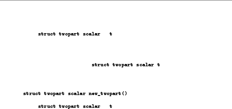
192 [M-2] struct — Structures
When a variable, argument, or returned value is a structure, however, you must explicitly declare it:
function makecalc()
{
t.n1 = t.n2 = 0
. . .
}
function clear_twopart( )
{
t.n1 = t.n2 = 0
}
{
t.n1 = t.n2 = 0
return(t)
}
In the functions above, we refer to variables t.n1 and t.n2. The Mata compiler cannot interpret
those names unless it knows the definition of the structure.
Aside: all structure references are resolved at compile time, not run time. That is, terms like t.n1 are
not stored in the compiled code and resolved during execution. Instead, the Mata compiler accesses
the structure definition when it compiles your code. The compiler knows that t.n1 refers to the first
element of the structure and generates efficient code to access it.
Declare structure variables to be scalars whenever possible
In our declarations, we code things like
struct twopart scalar t
and do not simply code
struct twopart t
although the simpler statement would be valid.
Structure variables can be scalars, vectors, or matrices; when you do not say which, matrix is assumed.
Most uses of structures are as scalars, and the compiler will generate more efficient code if you tell
it that the structures are scalars. Also, when you use structure vectors or matrices, there is an extra
step you need to fill in, as described in the next section.
Vectors and matrices of structures
Just as you can have real scalars, vectors, or matrices, you can have structure scalars, vectors, or
matrices. The following are all valid:

[M-2] struct — Structures 193
struct twopart scalar t
struct twopart vector t
struct twopart rowvector t
struct twopart colvector t
struct twopart matrix t
In a struct twopart matrix, every element of the matrix is a separate structure. Say that the
matrix were 2 ×3. Then you could refer to any of the following variables,
t[1,1].n1
t[1,2].n1
t[1,3].n1
t[2,1].n1
t[2,2].n1
t[2,3].n1
and similarly for t[i,j].n2.
If struct twopart also contained a matrix X, then
t[i,j].X
would refer to the (i,j)th matrix.
t[i,j].X[k,l]
would refer to the (k,l)th element of the (i,j)th matrix.
If tis to be a 2 ×3 matrix, you must arrange to make it 2 ×3. After the declaration
struct twopart matrix t
tis 0 ×0. This result is no different from the situation where tis a real matrix and after
declaration, tis 0 ×0.
Whether tis a real matrix or a struct twopart matrix, you allocate tby assignment. Let’s
pretend that tis a real matrix. There are three solutions to the allocation problem:
(1) t=x
(2) t = somefunction(. . . )
(3) t = J(r,c,v)
All three are so natural that you do not even think of them as allocation; you think of them as
definition.
The situation with structures is the same.
Let’s take each in turn.
1. xcontains a 2 ×3struct twopart. You code
t=x
and now tcontains a copy of x.tis 2 ×3.

194 [M-2] struct — Structures
2. somefunction(. . . )returns a 2 ×3struct twopart. You code
t = somefunction(. . . )
and now tcontains the 2 ×3 result.
3. Mata function J(r,c,v)returns an r×cmatrix, every element of which is set to v. So
pretend that variable tpc contains a struct twopart scalar. You code
t = J(2, 3, tpc)
and now tis 2 ×3, every element of which is a copy of tpc. Here is how you might do
that:
function . . . (. . . )
{
struct twopart scalar tpc
struct twopart matrix t
. . .
t = J(2, 3, tpc)
. . .
}
Finally, there is a fourth way to create structure vectors and matrices. When you defined
struct twopart {
real scalar n1, n2
}
Mata not only recorded the structure definition but also created a function named twopart() that
returns a struct twopart. Thus, rather than enduring all the rigmarole of creating a matrix from
a preallocated scalar, you could simply code
t = J(2, 3, twopart())
In fact, the function twopart() that Mata creates for you allows 0, 1, or 2 arguments:
twopart() returns a 1 ×1struct twopart
twopart(r)returns an r×1struct twopart
twopart(r,c)returns an r×cstruct twopart
so you could code
t = twopart(2, 3)
or you could code
t = J(2, 3, twopart())
and whichever you code makes no difference.
Either way, what is in t? Each element contains a separate struct twopart. In each struct
twopart, the scalars have been set to missing (.,"", or NULL, as appropriate), the vectors and row
vectors have been made 1 ×0, the column vectors 0 ×1, and the matrices 0 ×0.

[M-2] struct — Structures 195
Structures of structures
Structures may contain other structures:
struct twopart {
real scalar n1, n2
}
struct pair_of_twoparts {
struct twopart scalar t1, t2
}
If twere a struct pair of twoparts scalar, then the members of twould be
t.t1 astruct twopart scalar
t.t2 astruct twopart scalar
t.t1.n1 areal scalar
t.t1.n2 areal scalar
t.t2.n1 areal scalar
t.t2.n2 areal scalar
You may also create structures of structures of structures, structures of structures of structures of
structures, and so on. You may not, however, include a structure in itself:
struct recursive {
. . .
struct recursive scalar r
. . .
}
Do you see how, even in the scalar case, struct recursive would require an infinite amount of
memory to store?
Pointers to structures
What you can do is this:
struct recursive {
. . .
pointer(struct recursive scalar) scalar r
. . .
}
Thus, if rwere a struct recursive scalar, then *r.r would be the next structure, or r.r would
be NULL if there were no next structure. Immediately after allocation, r.r would equal NULL.
In this way, you may create linked lists.
Mata provides operator -> for accessing members of pointers to structures.
Let rec be a struct recursive, and assume that struct recursive also had member real
scalar n, so that rec.n would be rec’s nvalue. The value of the next structure’s nwould be
rec.r->n (assuming rec.r!=NULL).

196 [M-2] struct — Structures
The syntax of -> is
exp1 -> exp2
where exp1 evaluates to a structure pointer and exp2 indexes the structure.
Operators and functions for use with structure members
All operators, all functions, and all features of Mata work with members of structures. That is, given
struct example {
real scalar n
real matrix X
}
function . . . (. . . )
{
real scalar rs
real matrix rm
struct example scalar ex
. . .
}
then ex.n and ex.X may be used anyplace rs and rm would be valid.
Operators and functions for use with entire structures
Some operators and functions can be used with entire structures, not just the structure’s elements.
Given
struct mystruct scalar ex1, ex2, ex3, ex4
struct mystruct matrix E, F, G
1. You may use == and != to test for equality:
if (ex1==ex2) . . .
if (ex1!=ex2) . . .
Two structures are equal if their members are equal.
In the example, struct mystruct itself contains no substructures. If it did, the definition
of equality would include checking the equality of substructures, sub-substructures, etc.
In the example, ex1 and ex2 are scalars. If they were matrices, each element would be
compared, and the matrices would be equal if the corresponding elements were equal.
2. You may use :== and :!= to form pattern matrices of equality and inequality.
3. You may use the comma and backslash operators to form vectors and matrices of structures:
ex = ex1, ex2 \ ex3, ex4
4. You may use &to obtain pointers to structures:
ptr_to_ex1 = &ex1

[M-2] struct — Structures 197
5. You may use subscripting to access and copy structure members:
ex1 = E[1,2]
E[1,2] = ex1
F = E[2,.]
E[2,.] = F
G = E[|1,1\2,2|]
E[|1,1\2,2|] = G
6. You may use the rows() and cols() functions to obtain the number of rows and columns
of a matrix of structures.
7. You may use eltype() and orgtype() with structures. eltype() returns struct;
orgtype() returns the usual results.
8. You may use most functions that start with the letters is, as in isreal(),iscomplex(),
isstring(), etc. These functions return 1 if true and 0 if false and with structures, usually
return 0.
9. You may use swap() with structures.
Listing structures
To list the contents of a structure variable, as for debugging purposes, use function liststruct();
see [M-5]liststruct( ).
Using the default, unassigned-expression method to list structures is not recommended, because all
that is shown is a pointer value instead of the structure itself.
Use of transmorphics as passthrus
Atransmorphic matrix can theoretically hold anything, so when we told you that structures had
to be explicitly declared, that was not exactly right. Say that function twopart() returns a struct
twopart scalar. You could code
x = twopart()
without declaring x(or declaring it transmorphic), and that would not be an error. What you could
not do would be to then refer to x.n1 or x.n2, because the compiler would not know that xcontains
astruct twopart and so would have no way of interpreting the variable references.
This property can be put to good use in implementing handles and passthrus.
Say that you are implementing a complicated system. Just to fix ideas, we’ll pretend that the system
finds the maximum of user-specified functions and that the system has many bells and whistles. To
track a given problem, let’s assume that your system needs many variables. One variable records the
method to be used. Another records whether numerical derivatives are to be used. Another records
the current gradient vector. Another records the iteration count, and so on. There might be hundreds
of these variables.

198 [M-2] struct — Structures
You bind all of these variables together in one structure:
struct maxvariables {
real scalar method
real scalar use_numeric_d
real vector gradient
real scalar iteration
. . .
}
You design a system with many functions, and some functions call others, but because all the status
variables are bound together in one structure, it is easy to pass the values from one function to another.
You also design a system that is easy to use. It starts by the user “opening” a problem,
handle = maximize_open()
and from that point on the user passes the handle around to the other maximize routines:
maximize_set_use_numeric_d(handle, 1)
maximize_set_function_to_max(handle, &myfunc())
. . .
maximize_maximize_my_function(handle)
In this way, you, the programmer of this system, can hold on to values from one call to the next,
and you can change the values, too.
What you never do, however, is tell the user that the handle is a struct maxvariables. You just
tell the user to open a problem by typing
handle = maximize_open()
and then to pass the handle returned to the other maximize *() routines. If the user feels that he
must explicitly declare the handle, you tell him to declare it:
transmorphic scalar handle
What is the advantage of this secrecy? You can be certain that the user never changes any of the
values in your struct maxvariables because the compiler does not even know what they are.
Thus you have made your system more robust to user errors.
Saving compiled structure definitions
You save compiled structure definitions just as you save compiled function definitions; see [M-3]mata
mosave and [M-3]mata mlib.
When you define a structure, such as twopart,
struct twopart {
real scalar n1, n2
}
that also creates a function, twopart(), that creates instances of the structure.
Saving twopart() in a .mo file, or in a .mlib library, saves the compiled definition as well. Once
twopart() has been saved, you may write future programs without bothering to define struct
twopart. The definition will be automatically found.

[M-2] struct — Structures 199
Saving structure variables
Variables containing structures may be saved on disk just as you would save any other variable.
No special action is required. See [M-3]mata matsave and see the function fputmatrix() in
[M-5]fopen( ).mata matsave and fputmatrix() both work with structure variables, although their
entries do not mention them.
Reference
Gould, W. W. 2007. Mata Matters: Structures.Stata Journal 7: 556–570.
Also see
[M-2]declarations — Declarations and types
[M-2]intro — Language definition

Title
[M-2] subscripts — Use of subscripts
Syntax Description Remarks and examples Conformability
Diagnostics Reference Also see
Syntax
x[real vector r,real vector c]
x[|real matrix sub|]
Subscripts may be used on the left or right of the equal-assignment operator.
Description
Subscripts come in two styles.
In [subscript]syntax—called list subscripts—an element or a matrix is specified:
x[1,2] the 1,2 element of x; a scalar
x[(1\3\2), (4,5)] the 3 ×2 matrix composed of rows 1, 3, and 2
and columns 4 and 5 of x:
x14 x15
x34 x35
x24 x25
In [|subscript|] syntax—called range subscripts—an element or a contiguous submatrix is specified:
x[|1,2|] same as x[1,2]; a scalar
x[|2,3 \ 4,7|] 3×4 submatrix of x:
x23 x24 x25 x26 x27
x33 x34 x35 x36 x37
x43 x44 x45 x46 x47
Both style subscripts may be used in expressions and may be used on the left-hand side of the
equal-assignment operator.
Remarks and examples
Remarks are presented under the following headings:
List subscripts
Range subscripts
When to use list subscripts and when to use range subscripts
A fine distinction
200

[M-2] subscripts — Use of subscripts 201
List subscripts
List subscripts—also known simply as subscripts—are obtained when you enclose the subscripts in
square brackets, [and ]. List subscripts come in two basic forms:
x[ivec,jvec]matrix composed of rows ivec and columns jvec of matrix x
v[kvec]vector composed of elements kvec of vector v
where ivec,jvec,kvec may be a vector or a scalar, so the two basic forms include
x[i,j]scalar i,jelement
x[i,jvec]row vector of row i, elements jvec
x[ivec,j]column vector of column j, elements ivec
v[k]scalar kth element of vector v
Also missing value may be specified to mean all the rows or all the columns:
x[i,.] row vector of row iof x
x[., j]column vector of column jof x
x[ivec,.] matrix of rows ivec, all columns
x[., jvec]matrix of columns jvec, all rows
x[.,.] the entire matrix
Finally, Mata assumes missing value when you omit the argument entirely:
x[i,] same as x[i,.]
x[ivec,] same as x[ivec,.]
x[, j]same as x[., j]
x[, jvec]same as x[., jvec]
x[,] same as x[.,.]
Good style is to specify ivec as a column vector and jvec as a row vector, but that is not required:
x[(1\2\3), (1,2,3)] good style
x[(1,2,3), (1,2,3)] same as x[(1\2\3), (1,2,3)]
x[(1\2\3), (1\2\3)] same as x[(1\2\3), (1,2,3)]
x[(1,2,3), (1\2\3)] same as x[(1\2\3), (1,2,3)]
Similarly, good style is to specify kvec as a column when vis a column vector and to specify kvec
as a row when vis a row vector, but that is not required and what is returned is a column vector if
vis a column and a row vector if vis a row:
rowv[(1,2,3)] good style for specifying row vector
rowv[(1\2\3)] same as rowv[(1,2,3)]
colv[(1\2\3)] good style for specifying column vector
colv[(1,2,3)] same as colv[(1\2\3)]

202 [M-2] subscripts — Use of subscripts
Subscripts may be used in expressions following a variable name:
first = list[1]
multiplier = x[3,4]
result = colsum(x[,j])
Subscripts may be used following an expression to extract a submatrix from a result:
allneeded = invsym(x)[(1::4), .] * multiplier
Subscripts may be used on the left-hand side of the equal-assignment operator:
x[1,1] = 1
x[1,.] = y[3,.]
x[(1::4), (1..4)] = I(4)
Range subscripts
Range subscripts appear inside the difficult to type [| and |] brackets. Range subscripts come in
four basic forms:
x[|i,j|] i,jelement; same result as x[i,j]
v[|k|] kth element of vector; same result as v[k]
x[|i,j\k,l|] submatrix, vector, or scalar formed using (i,j) as top-left
corner and (k,l) as bottom-right corner
v[|i\k|] subvector or scalar of elements ithrough k; result is
row vector if vis row vector, column vector if vis column
vector
Missing value may be specified for a row or column to mean all rows or all columns when a 1 ×2
or 1 ×1 subscript is specified:
x[|i,.|] row iof x; same as x[i,.]
x[|., j|] column jof x; same as x[., j]
x[|.,.|] entire matrix; same as x[.,.]
v[|.|] entire vector; same as v[.]
Also missing may be specified to mean the number of rows or the number of columns of the matrix
being subscripted when a 2 ×2 subscript is specified:
x[|1,2 \ 4,.|] equivalent to x[|1,2 \ 4,cols(x)|]
x[|1,2 \ .,3|] equivalent to x[|1,2 \ rows(x),3|]
x[|1,2 \ .,.|] equivalent to x[|1,2 \ rows(x),cols(x|]
With range subscripts, what appears inside the square brackets is in all cases interpreted as a matrix
expression, so in
sub = (1,2)
. . . x[|sub|] . . .

[M-2] subscripts — Use of subscripts 203
x[sub] refers to x[1,2].
Range subscripts may be used in all the same contexts as list subscripts; they may be used in
expressions following a variable name
submat = result[|1,1 \ 3,3|]
they may be used to extract a submatrix from a calculated result
allneeded = invsym(x)[|1,1 \ 4,4|]
and they may be used on the left-hand side of the equal-assignment operator:
x[|1,1 \ 4,4|] = I(4)
When to use list subscripts and when to use range subscripts
Everything a range subscript can do, a list subscript can also do. The one seemingly unique feature
of a range subscript,
x[|i1,j1 \i2,j2|]
is perfectly mimicked by
x[(i1::i2), (j1..j2)]
The range-subscript construction, however, executes more quickly, and so that is the purpose of
range subscripts: to provide a fast way to extract contiguous submatrices. In all other cases, use list
subscripts because they are faster.
Use list subscripts to refer to scalar values:
result = x[1,3]
x[1,3] = 2
Use list subscripts to extract entire rows or columns:
obs = x[., 3]
var = x[4, .]
Use list subscripts to permute the rows and columns of matrices:
: x = (1,2,3,4 \ 5,6,7,8 \ 9,10,11,12)
: y = x[(1\3\2), .]
: y
1234
1 1234
2 9 10 11 12
3 5678
: y = x[., (1,3,2,4)]
: y
1234
1 1324
2 5768
3 9 11 10 12
: y=x[(1\3\2), (1,3,2,4)]

204 [M-2] subscripts — Use of subscripts
: y
1234
1 1324
2 9 11 10 12
3 5768
Use list subscripts to duplicate rows or columns:
: x = (1,2,3,4 \ 5,6,7,8 \ 9,10,11,12)
: y = x[(1\2\3\1), .]
: y
1234
1 1234
2 5678
3 9 10 11 12
4 1234
: y = x[., (1,2,3,4,2)]
: y
12345
1 12342
2 56786
3 9 10 11 12 10
: y = x[(1\2\3\1), (1,2,3,4,2)]
: y
12345
1 12342
2 56786
3 9 10 11 12 10
4 12342
A fine distinction
There is a fine distinction between x[i,j]and x[|i,j|]. In x[i,j], there are two arguments, iand
j. The comma separates the arguments. In x[|i,j|], there is one argument: i,j. The comma is the
column-join operator.
In Mata, comma means mostly the column-join operator:
newvec = oldvec, addedvalues
qsum = (x,1)’(x,1)
There are, in fact, only two exceptions. When you type the arguments for a function, the comma
separates one argument from the next:
result = f(a,b,c)
In the above example, f() receives three arguments: a,b, and c. If we wanted f() to receive one
argument, (a,b,c), we would have to enclose the calculation in parentheses:
result = f((a,b,c))

[M-2] subscripts — Use of subscripts 205
That is the first exception. When you type the arguments inside a function, comma means argument
separation. You get back to the usual meaning of comma—the column-join operator—by opening
another set of parentheses.
The second exception is in list subscripting:
x[i,j]
Inside the list-subscript brackets, comma means argument separation. That is why you have seen us
type vectors inside parentheses:
x[(1\2\3),(1,2,3)]
These are the two exceptions. Range subscripting is not an exception. Thus in
x[| i,j|]
there is one argument, i,j. With range subscripts, you may program constructs such as
IJ = (i,j)
RANGE = (1,2 \ 4,4)
. . .
. . . x[|IJ|] . . . x[|RANGE|] . . .
You may not code in this way with list subscripts. In particular, x[IJ] would be interpreted as a
request to extract elements iand jfrom vector x, and would be an error otherwise. x[RANGE] would
always be an error.
We said earlier that list subscripts x[i,j]are a little faster than range subscripts x[|i,j|]. That is
true, but if IJ=(i,j)already, x[|IJ|] is faster than x[i,j]. You would, however, have to execute
many millions of references to x[|IJ|] before you could measure the difference.
Conformability
x[i,j]:
x:r×c
i:m×1 or 1 ×m(does not matter which)
j: 1 ×nor n×1 (does not matter which)
result:m×n
x[i, .]:
x:r×c
i:m×1 or 1 ×m(does not matter which)
result:m×c
x[., j]:
x:r×c
j: 1 ×nor n×1 (does not matter which)
result:r×n
x[., .]:
x:r×c
result:r×c

206 [M-2] subscripts — Use of subscripts
x[i]:x:n×1 1 ×n
i:m×1 or 1 ×m1×mor m×1
result:m×1 1 ×m
x[.]:x:n×1 1 ×n
result:n×1 1 ×n
x[|k|]:x:r×c
k: 1 ×2
result: 1 ×1 if k[1]<. and k[2]<.
r×1 if k[1]>=. and k[2]<.
1×cif k[1]<. and k[2]>=.
r×cif k[1]>=. and k[2]>=.
x[|k|]:x:r×c
k: 2 ×2
result:k[2,1]-k[1,1]+1 ×k[2,2]-k[1,2]+1
(in the above formula, if k[2,1]>=., treat as if k[2,1]=r,
and similarly, if k[2,2]>=., treat as if k[2,2]=c)
x[|k|]:x:r×1 1 ×c
k: 2 ×1 2 ×1
result:k[2]-k[1]+1 ×1 1 ×k[2]-k[1]+1
(if k[2]>=., treat as (if k[2]>=., treat as
if k[2]=r) if k[2]=c)
Diagnostics
Both styles of subscripts abort with error if the subscript is out of range, if a reference is made to a
nonexisting row or column.
Reference
Gould, W. W. 2007. Mata Matters: Subscripting.Stata Journal 7: 106–116.
Also see
[M-2]intro — Language definition

Title
[M-2] syntax — Mata language grammar and syntax
Syntax Description Remarks and examples Reference Also see
Syntax
The basic language syntax is
istmt
where
istmt := stmt
function name(farglist)fstmt
ftype name(farglist)fstmt
ftype function name(farglist)fstmt
stmt := nothing
;(meaning nothing)
version number
{stmt . . . }
exp
pragma pstmt
if (exp)stmt
if (exp)stmt else stmt
for (exp;exp;exp)stmt
while (exp)stmt
do stmt while (exp)
break
continue
label:
goto label
return
return(exp)
fstmt := stmt
type arglist
external type arglist
arglist := name
name()
name,arglist
name(), arglist
farglist := nothing
efarglist
efarglist := felement
felement,efarglist
|felement
|felement,efarglist
207

208 [M-2] syntax — Mata language grammar and syntax
felement := name
type name
name()
type name()
ftype := type
void
type := eltype
orgtype
eltype orgtype
eltype := transmorphic
string
numeric
real
complex
pointer
pointer(ptrtype)
orgtype := matrix
vector
rowvector
colvector
scalar
ptrtype := nothing
type
type function
function
pstmt := unset name
unused name
name := identifier up to 32 characters long
label := identifier up to 8 characters long
exp := expression as defined in [M-2]exp
Description
Mata is a C-like compiled-into-pseudocode language with matrix extensions and run-time linking.
Remarks and examples
Remarks are presented under the following headings:
Treatment of semicolons
Types and declarations
Void matrices
Void functions
Operators
Subscripts
Implied input tokens
Function argument-passing convention
Passing functions to functions
Optional arguments

[M-2] syntax — Mata language grammar and syntax 209
After reading [M-2]syntax, see [M-2]intro for a list of entries that give more explanation of what is
discussed here.
Treatment of semicolons
Semicolon (;) is treated as a line separator. It is not required, but it may be used to place two
statements on the same physical line:
x=1;y=2;
The last semicolon in the above example is unnecessary but allowed.
Single statements may continue onto more than one line if the continuation is obvious. Take “obvious”
to mean that there is a hanging open parenthesis or a hanging dyadic operator; for example,
x=(
3)
x = x +
2
See [M-2]semicolons for more information.
Types and declarations
The type of a variable or function is described by
eltype orgtype
where eltype and orgtype are each one of
eltype orgtype
transmorphic matrix
numeric vector
real rowvector
complex colvector
string scalar
pointer
For example, a variable might be real scalar, or complex matrix, or string vector.
Mata also has structures—the eltype is struct name—but these are not discussed here. For a
discussion of structures, see [M-2]struct.
Mata also has classes—the eltype is class name—but these are not discussed here. For a discussion
of classes, see [M-2]class.
Declarations are optional. When the type of a variable or function is not declared, it is assumed to
be a transmorphic matrix. In particular:
1. eltype specifies the type of the elements. When eltype is not specified, transmorphic is
assumed.
210 [M-2] syntax — Mata language grammar and syntax
2. orgtype specifies the organization of the elements. When orgtype is not specified, matrix
is assumed.
All types are special cases of transmorphic matrix.
The nesting of eltypes is
transmorphic
numeric string pointer
real complex
orgtypes amount to nothing more than a constraint on the number of rows and columns of a matrix:
orgtype Constraint
matrix r≥0 and c≥0
vector r=1 and c≥0 or r≥0 and c=1
rowvector r=1 and c≥0
colvector r≥0 and c=1
scalar r=1 and c=1
See [M-2]declarations.
Void matrices
A matrix (vector, row vector, or column vector) that is 0 ×0, r×0, or 0 ×cis said to be void;
see [M-2]void.
The function J(r,c,val)returns an r×cmatrix with each element containing val; see [M-5]J( ).
J() can be used to create void matrices.
See [M-2]void.
Void functions
Rather than eltype orgtype, a function can be declared to return nothing by being declared to return
void:
void function example(matrix A)
{
real scalar i
for (i=1; i<=rows(A); i++) A[i,i] = 1
}
A function that returns nothing (does not include a return(exp)statement), in fact returns J(0, 0, .),
and the above function could equally well be coded as

[M-2] syntax — Mata language grammar and syntax 211
void function example(matrix A)
{
real scalar i
for (i=1; i<=rows(A); i++) A[i,i] = 1
return(J(0, 0, .))
}
or
void function example(matrix A)
{
real scalar i
for (i=1; i<=rows(A); i++) A[i,i] = 1
return(J(0,0,.))
}
Therefore, void also is a special case of transmorphic matrix (it is in fact a 0 ×0real
matrix). Since declarations are optional (but recommended both for reasons of style and for reasons
of efficiency), the above function could also be coded as
function example(A)
{
for (i=1; i<=rows(A); i++) A[i,i] = 1
}
See [M-2]declarations.
Operators
Mata provides the usual assortment of operators; see [M-2]exp.
The monadic prefix operators are
- ! ++ -- & *
Prefix operators &and *have to do with pointers; see [M-2]pointers.
The monadic postfix operators are
0++ --
Note the inclusion of postfix operator 0for transposition. Also, for Zcomplex, Z0returns the conjugate
transpose. If you want the transposition without conjugation, see [M-5]transposeonly( ).
The dyadic operators are
= ? \ :: , .. | & == >= <= < >
!=+-*#^
Also, && and || are included as synonyms for &and |.
The operators == and != do not require conformability, nor do they require that the matrices be of
the same type. In such cases, the matrices are unequal (== is false and != is true). For complex
arguments, <,<=,>, and >= refer to length of the complex vector. == and !=, however, refer not to
length but to actual components. See [M-2]op logical.

212 [M-2] syntax — Mata language grammar and syntax
The operators ,and \are the row-join and column-join operators. (1,2,3) constructs the row vector
(1,2,3). (1\2\3) constructs the column vector (1,2,3)0.(1,2\3,4) constructs the matrix with first
row (1,2) and second row (3,4). a,bjoins two scalars, vectors, or matrices rowwise. a\bjoins two
scalars, vectors, or matrices columnwise. See [M-2]op join.
.. and :: refer to the row-to and column-to operators. 1..5 is (1,2,3,4,5). 1::5 is (1\2\3\4\5).
5..1 is (5,4,3,2,1). 5::1 is (5\4\3\2\1). See [M-2]op range.
For |,&,==,>=,<=,<,>,!=,+,-,*,/, and ^, there is :op at precedence just below op. These
operators perform the elementwise operation. For instance, A*Brefers to matrix multiplication; A:*B
refers to elementwise multiplication. Moreover, elementwise is generalized to cases where Aand B
do not have the same number of rows and the same number of columns. For instance, if Ais a 1 ×
crow vector and Bis a r×cmatrix, then ||Cij || =||Aj|| ∗ ||Bij || is returned. See [M-2]op colon.
Subscripts
A[i,j]returns the i,jelement of A.
A[k]returns A[1,k]if Ais 1 ×cand A[k,1] if Ais r×1. That is, in addition to declared vectors,
any 1 ×cmatrix or r×1 matrix may be subscripted by one index. Similarly, any vector can be
subscripted by two indices.
i,j, and kmay be vectors as well as scalars. For instance, A[(3\4\5), 4] returns a 3 ×1 column
vector containing rows 3 to 5 of the 4th column.
i,j, and kmay be missing value. A[., 4] returns a column vector of the 4th column of A.
The above subscripts are called list-style subscripts. Mata provides a second format called range-style
subscripts that is especially useful for selecting submatrices. A[|3,3\5,5|] returns the 3 ×3
submatrix of Astarting at A[3,3].
See [M-2]subscripts.
Implied input tokens
Before interpreting and compiling a line, Mata makes the following substitutions to what it sees:
Input sequence Interpretation
0name 0*name
[, [.,
,] ,.]
Hence, coding X0Zis equivalent to coding X0*Z, and coding x = z[1,] is equivalent to coding x =
z[1,.].

[M-2] syntax — Mata language grammar and syntax 213
Function argument-passing convention
Arguments are passed to functions by address, also known as by name or by reference. They are not
passed by value. When you code
. . . f(A) . . .
it is the address of Athat is passed to f(), not a copy of the values in A.f() can modify A.
Most functions do not modify their arguments, but some do. lud(A,L,U,p), for instance, calculates
the LU decomposition of A. The function replaces the contents of L,U, and pwith matrices such that
L[p,]*U=A.
Oldtimers will have heard of the FORTRAN programmer who called a subroutine and passed to it
a second argument of 1. Unbeknownst to him, the subroutine changed its second argument, with
the result that the constant 1 was changed throughout the rest of his code. That cannot happen in
Mata. When an expression is passed as an argument (and constants are expressions), a temporary
variable containing the evaluation is passed to the function. Modifications to the temporary variable
are irrelevant because the temporary variable is discarded once the function returns. Thus if f()
modifies its second argument and you call it by coding f(A,2), because 2 is copied to a temporary
variable, the value of the literal 2 will remain unchanged on the next call.
If you call a function with an expression that includes the assignment operator, it is the left-hand side
of the expression that is passed. That is, coding
f(a, b=c)
has the same result as coding
b=c
f(a, b)
If function f() changes its second argument, it will be band not cthat is modified.
Also, Mata attempts not to create unnecessary copies of matrices. For instance, consider
function changearg(x) x[1,1] = 1
changearg(mymat) changes the 1,1 element of mymat to 1. Now let us define
function cp(x) return(x)
Coding changearg(cp(mymat)) would still change mymat because cp() returned xitself. On the
other hand, if we defined cp() as
function cp(x)
{
matrix t
t=x
return(t)
}
then coding changearg(cp(mymat)) would not change mymat. It would change a temporary matrix
which would be discarded once changearg() returned.

214 [M-2] syntax — Mata language grammar and syntax
Passing functions to functions
One function may receive another function as an argument using pointers. One codes
function myfunc(pointer(function) f, a, b)
{
. . . (*f)(a) . . . (*f)(b) . . .
}
although the pointer(function) declaration, like all declarations, is optional. To call myfunc()
and tell it to use function prima() for f(), and 2 and 3 for aand b, one codes
myfunc(&prima(), 2, 3)
See [M-2]ftof and [M-2]pointers.
Optional arguments
Functions may be coded to allow receiving a variable number of arguments. This is done by placing
a vertical or bar (|) in front of the first argument that is optional. For instance,
function mynorm(matrix A, |scalar power)
{
. . .
}
The above function may be called with one matrix or with a matrix followed by a scalar.
The function args() (see [M-5]args( )) can be used to determine the number of arguments received
and to set defaults:
function mynorm(matrix A, |scalar power)
{
. . .
(args()==1) power = 2
. . .
}
See [M-2]optargs.
Reference
Gould, W. W. 2005. Mata Matters: Translating Fortran.Stata Journal 5: 421–441.
Also see
[M-2]intro — Language definition

Title
[M-2] version — Version control
Syntax Description Remarks and examples Also see
Syntax
Syntax 1
. version #.#
. mata:
:. . .
: function name(. . . )
: {
:. . .
: }
:. . .
: end
Syntax 2
: function name(. . . )
: {
: version #.#
:. . .
: }
Description
In syntax 1, Stata’s version command (see [P]version) sets the version before entering Mata. This
specifies both the compiler and library versions to be used. Syntax 1 is recommended.
In syntax 2, Mata’s version command sets the version of the library functions that are to be used.
Syntax 2 is rarely used.
Remarks and examples
Remarks are presented under the following headings:
Purpose of version control
Recommendations for do-files
Recommendations for ado-files
Compile-time and run-time versioning
215

216 [M-2] version — Version control
Purpose of version control
Mata is under continual development, which means not only that new features are being added but
also that old features sometimes change how they work. Old features changing how they work is
supposedly an improvement—it generally is—but that also means old programs might stop working
or, worse, work differently.
version provides the solution.
If you are working interactively, nothing said here matters.
If you use Mata in do-files or ado-files, we recommend that you set version before entering Mata.
Recommendations for do-files
The recommendation for do-files that use Mata is the same as for do-files that do not use Mata:
specify the version number of the Stata you are using on the top line:
begin myfile.do
version 13
. . .
end myfile.do
To determine the number that should appear after version, type about at the Stata prompt:
. about
Stata/SE 13.0
(output omitted )
We are using Stata 13.0.
Coding version 13 will not benefit us today but, in the future, we will be able to rerun our do-file
and obtain the same results.
By the way, a do-file is any file that you intend to execute using Stata’s do or run commands (see
[R]do), regardless of the file suffix. Many users (us included) save Mata source code in .mata files
and then type do myfile.mata to compile. .mata files are do-files; we include the version line:
begin myfile.mata
version 13
mata:
. . .
end
end myfile.mata
Recommendations for ado-files
Mata functions may be included in ado-files; see [M-1]ado. In such files, set version before entering
Mata along with, as usual, setting the version at the top of your program:

[M-2] version — Version control 217
begin myfile.ado
program myfile
version 13 ←as usual
. . .
end
version 13 ←new
mata:
. . .
end
end myfile.ado
Compile-time and run-time versioning
What follows is detail. We recommend always following the recommendations above.
There are actually two version numbers that matter—the version number set at the time of compilation,
which affects how the source code is interpreted, and the version of the libraries used to supply
subroutines at the time of execution.
The version command that we used in the previous sections is in fact Stata’s version command
(see [P]version), and it sets both versions:
. version 13
. mata:
: function example()
: {
:. . .
: }
: end
In the above, we compile example() by using the version 13 syntax of the Mata language, and any
functions example() calls will be the 13 version of those functions. Setting version 13 before
entering Mata ensured all of that.
In the following example, we compile using version 13 syntax and use version 13.2 functions:
. version 13
. mata:
: function example()
: {
: version 13.2
:. . .
: }
: end
In the following example, we compile using version 13.2 syntax and use version 13 functions:
. version 13.2
. mata:
: function example()
: {
: version 13
:. . .
: }
: end


Title
[M-2] void — Void matrices
Syntax Description Remarks and examples Also see
Syntax
J(0, 0, .) 0×0 real matrix
J(r, 0, .) r×0 real matrix
J(0, c, .) 0×creal matrix
J(0, 0, 1i) 0×0 complex matrix
J(r, 0, 1i) r×0 complex matrix
J(0, c, 1i) 0×ccomplex matrix
J(0, 0, "") 0×0 string matrix
J(r, 0, "") r×0 string matrix
J(0, c, "") 0×cstring matrix
J(0, 0, NULL) 0×0 pointer matrix
J(r, 0, NULL) r×0 pointer matrix
J(0, c, NULL) 0×cpointer matrix
Description
Mata allows 0 ×0, r×0, and 0 ×cmatrices. These matrices are called void matrices.
Remarks and examples
Remarks are presented under the following headings:
Void matrices, vectors, row vectors, and column vectors
How to read conformability charts
Void matrices, vectors, row vectors, and column vectors
Void matrices contain nothing, but they have dimension information (they are 0 ×0, r×0, or 0 ×
c) and have an eltype (which is real,complex,string, or pointer):
1. A matrix is said to be void if it is 0 ×0, r×0, or 0 ×c.
2. A vector is said to be void if it is 0 ×1 or 1 ×0.
3. A column vector is said to be void if it is 0 ×1.
4. A row vector is said to be void if it is 1 ×0.
5. A scalar cannot be void because it is, by definition, 1 ×1.
219

220 [M-2] void — Void matrices
The function J(r,c,val)creates r×cmatrices containing val; see [M-5]J( ).J() can be used to
manufacture void matrices by specifying rand/or cas 0. The value of the third argument does not
matter, but its eltype does:
1. J(0,0,.) creates a real 0 ×0 matrix, as will J(0,0,1) and as will J() with any real
third argument.
2. J(0,0,1i) creates a 0 ×0 complex matrix, as will J() with any complex third argument.
3. J(0,0,"") creates 0 ×0 string matrices, as will J() with any string third argument.
4. J(0,0,NULL) creates 0 ×0 pointer matrices, as will J() with any pointer third argument.
In fact, one rarely needs to manufacture such matrices because they arise naturally in extreme cases.
Similarly, one rarely needs to include special code to handle void matrices because such matrices
handle themselves. Loops vanish when the number of rows or columns are zero.
How to read conformability charts
In general, not only is no emphasis placed on how functions and operators deal with void matrices,
no mention is even made of the fact. Instead, the information is buried in the Conformability section
located near the end of the function’s or operator’s manual entry.
For instance, the conformability chart for some function might read
somefunction(A,B,v):
A:r×c
B:c×k
v: 1 ×kor k×1
result:r×k
Among other things, the chart above is stating how somefunction() handles void matrices. Amust
be r×c. That chart does not say
A:r×c,r>0, c>0
and that is what it would have said if somefunction() did not allow Ato be void. Hence, Amay
be 0 ×0, 0 ×c, or r×0.
Similarly, Bmay be void as long as rows(B)==cols(A).vmay be void if cols(B)==0. The
returned result will be void if rows(A)==0 or cols(B)==0.
Interestingly, somefunction() can produce a nonvoid result from void input. For instance, if A
were 5 ×0 and B, 0 ×3, a 5 ×3 result would be produced. It is interesting to speculate what would
be in that 5 ×3 result. Probably, if we knew what somefunction() did, it would be obvious to us,
but if it were not, the following section, Diagnostics, would state what the surprising result would be.
As a real example, see [M-5]trace( ).trace() will take the trace of a 0 ×0 matrix. The result is
0. Or see multiplication (*)in[M-2]op arith. One can multiply a k×0 matrix by a 0 ×mmatrix
to produce a k×mresult. The matrix will contain zeros.
Also see
[M-2]intro — Language definition

Title
[M-2] while — while (exp) stmt
Syntax Description Remarks and examples Also see
Syntax
while (exp)stmt
while (exp) {
stmts
}
where exp must evaluate to a real scalar.
Description
while executes stmt or stmts zero or more times. The loop continues as long as exp is not equal to
zero.
Remarks and examples
To understand while, enter the following program
function example(n)
{
i=1
while (i<=n) {
printf("i=%g\n", i)
i++
}
printf("done\n")
}
and run example(3),example(2),example(1),example(0), and example(-1).
One common use of while is to loop until convergence:
while (mreldif(a, lasta)>1e-10) {
lasta = a
a = . . .
}
221

[M-3] Commands for controlling Mata
223

Title
[M-3] intro — Commands for controlling Mata
Contents Description Remarks and examples Also see
Contents
Command for invoking Mata from Stata:
[M-3] Entry Command Description
mata . mata invoke Mata
Once you are running Mata, you can use the following commands from the colon prompt:
[M-3] Entry Command Description
mata help :mata help execute help command
mata clear : mata clear clear Mata
mata describe : mata describe describe contents of Mata’s memory
mata memory : mata memory display memory-usage report
mata rename : mata rename rename matrix or function
mata drop : mata drop remove from memory matrix or function
mata mosave : mata mosave create object file
mata mlib : mata mlib create function library
mata matsave : mata matsave save matrices
mata matsave : mata matuse restore matrices
mata matsave : mata matdescribe describe contents of matrix file
mata which : mata which identify function
mata set : mata query display values of settable parameters
mata set : mata set set parameters
mata stata : mata stata execute Stata command
end : end exit Mata and return to Stata
225

226 [M-3] intro — Commands for controlling Mata
Description
When you type something at the Mata prompt, it is assumed to be a Mata statement—something that
can be compiled and executed—such as
: 2+3
5
The mata command, however, is different. When what you type is prefixed by the word mata, think
of yourself as standing outside of Mata and giving an instruction that affects the Mata environment
and the way Mata works. For instance, typing
: mata clear
says that Mata is to be cleared. Typing
: mata set matastrict on
says that Mata is to require that programs explicitly declare their arguments and their working variables;
see [M-2]declarations.
Remarks and examples
The mata command cannot be used inside functions. It would make no sense to code
function foo(. . . )
{
. . .
mata query
. . .
}
because mata query is something that can be typed only at the Mata colon prompt:
: mata query
(output omitted )
See [M-1]how.
Also see
[M-0]intro — Introduction to the Mata manual

Title
[M-3] end — Exit Mata and return to Stata
Syntax Description Remarks and examples Also see
Syntax
: end
Description
end exits Mata and returns to Stata.
Remarks and examples
When you exit from Mata back into Stata, Mata does not clear itself; so if you later return to Mata,
you will be right back where you were. See [M-3]mata.
Also see
[M-3]intro — Commands for controlling Mata
227

Title
[M-3] mata — Mata invocation command
Syntax Description Remarks and examples Also see
Syntax
The mata command documented here is for use from Stata. It is how you enter Mata. You type mata
at a Stata dot prompt, not a Mata colon prompt.
Syntax 1 Comment
mata no colon following mata
istmt
istmt if an error occurs, you stay in
.. mata mode
istmt
end you exit when you type end
Syntax 1 is the best way to use Mata interactively.
Syntax 2 Comment
mata: colon following mata
istmt
istmt if an error occurs, you are
.. dumped from mata
istmt
end otherwise, you exit when you type end
Syntax 2 is mostly used by programmers in ado-files.
Programmers want errors to stop everything.
Syntax 3 Comment
mata istmt rarely used
Syntax 3 is the single-line variant of syntax 1, but it is not useful.
Syntax 4 Comment
mata: istmt for use by programmers
Syntax 4 is the single-line variant of syntax 2, and it exists for the same reason
as syntax 2: for use by programmers in ado-files.
228

[M-3] mata — Mata invocation command 229
Description
The mata command invokes Mata. An istmt is something Mata understands; istmt stands for interactive
statement of Mata.
Remarks and examples
Remarks are presented under the following headings:
Introduction
The fine distinction between syntaxes 3 and 4
The fine distinction between syntaxes 1 and 2
Introduction
For interactive use, use syntax 1. Type mata (no colon), press Enter, and then use Mata freely. Type
end to return to Stata. (When you exit from Mata back into Stata, Mata does not clear itself; so if
you later type mata-followed-by-enter again, you will be right back where you were.)
For programming use, use syntax 2 or syntax 4. Inside a program or an ado-file, you can just call a
Mata function
program myprog
. . .
mata: utility("‘varlist’")
. . .
end
and you can even include that Mata function in your ado-file
begin myprog.ado
program myprog
. . .
mata: utility("‘varlist’")
. . .
end
mata:
function utility(string scalar varlist)
{. . .
}
end
end myprog.ado
or you could separately compile utility( ) and put it in a .mo file or in a Mata library.
The fine distinction between syntaxes 3 and 4
Syntaxes 3and 4are both single-line syntaxes. You type mata, perhaps a colon, and follow that with
the Mata istmt.
The differences between the two syntaxes is whether they allow continuation lines. With a colon, no
continuation line is allowed. Without a colon, you may have continuation lines.

230 [M-3] mata — Mata invocation command
For instance, let’s consider
function renorm(scalar a, scalar b)
{. . .
}
No matter how long the function, it is one istmt. Using mata:, if you were to try to enter that istmt,
here is what would happen:
. mata: function renorm(scalar a, scalar b)
<istmt> incomplete
r(197);
When you got to the end of the first line and pressed Enter, you got an error message. Using the
mata: command, the istmt must all fit on one line.
Now try the same thing using mata without the colon:
. mata function renorm(scalar a, scalar b)
> {
>. . .
> }
.
That worked! Single-line mata without the colon allows continuation lines and, on this score at least,
seems better than single-line mata with the colon. In programming contexts, however, this feature
can bite. Consider the following program fragment:
program example
. . .
mata utility("‘varlist’"
replace ‘x’ = . . .
. . .
end
We used mata without the colon, and we made an error: we forgot the close parenthesis. mata
without the colon will be looking for that close parenthesis and so will eat the next line—a line not
intended for Mata. Here we will get an error message because “replace ‘x’ = . . . ” will make no
sense to Mata, but that error will be different from the one we should have gotten. In the unlikely
worse case, that next line will make sense to Mata.
Ergo, programmers want to include the colon. It will make your programs easier to debug.
There is, however, a programmer’s use for single-line mata without the colon. In our sample ado-file
above when we included the routine utility(), we bound it in mata: and end. It would be
satisfactory if instead we coded
begin myprog.ado
program myprog
. . .
mata: utility("‘varlist’")
. . .
end
mata function utility(string scalar varlist)
{. . .
}
end myprog.ado

[M-3] mata — Mata invocation command 231
Using mata without the colon, we can omit the end. We admit we sometimes do that.
The fine distinction between syntaxes 1 and 2
Nothing said above about continuation lines applies to syntaxes 1and 2. The multiline mata, with or
without colon, always allows continuation lines because where the Mata session ends is clear enough:
end.
The difference between the two multiline syntaxes is whether Mata tolerates errors or instead dumps
you back into Stata. Interactive users appreciate tolerance. Programmers want strictness. Programmers,
consider the following (using mata without the colon):
program example2
. . .
mata
result = myfunc("‘varlist’")
st_local("n" result) /* <- mistake here */
result = J(0,0,"")
end
. . .
end
In the above example, we omitted the comma between "n" and result. We also used multiline
mata without the colon. Therefore, the incorrect line will be tolerated by Mata, which will merrily
continue executing our program until the end statement, at which point Mata will return control to
Stata and not tell Stata that anything went wrong! This could have serious consequences, all of which
could be avoided by substituting multiline mata with the colon.
Also see
[M-3]intro — Commands for controlling Mata

Title
[M-3] mata clear — Clear Mata’s memory
Syntax Description Remarks and examples Also see
Syntax
: mata clear
This command is for use in Mata mode following Mata’s colon prompt. To use this command from
Stata’s dot prompt, type
. mata: mata clear
Description
mata clear clears Mata’s memory, in effect resetting Mata. All functions, matrices, etc., are freed.
Remarks and examples
Stata can call Mata which can call Stata, which can call Mata, etc. In such cases, mata clear
releases only resources that are not in use by prior invocations of Mata.
Stata’s clear all command (see [D]clear) performs a mata clear, among other things.
See [M-3]mata drop for clearing individual matrices or functions.
Also see
[M-3]mata drop — Drop matrix or function
[M-3]intro — Commands for controlling Mata
232

Title
[M-3] mata describe — Describe contents of Mata’s memory
Syntax Description Option Remarks and examples
Diagnostics Also see
Syntax
: mata describe namelist , all
: mata describe using libname
where namelist is as defined in [M-3]namelists. If namelist is not specified, “* *()” is assumed.
This command is for use in Mata mode following Mata’s colon prompt. To use this command from
Stata’s dot prompt, type
. mata: mata describe . . .
Description
mata describe lists the names of the matrices and functions in memory, including the amount of
memory consumed by each.
mata describe using libname describes the contents of the specified .mlib library; see [M-3]mata
mlib.
Option
all specifies that automatically loaded library functions that happen to be in memory are to be
included in the output.
Remarks and examples
mata describe is often issued without arguments, and then everything in memory is described:
: mata describe
# bytes type name and extent
50 real matrix foo()
1,600 real matrix X[10,20]
8 real scalar x
233

234 [M-3] mata describe — Describe contents of Mata’s memory
mata describe using libname lists the functions stored in a .mlib library:
: mata describe using lmatabase
# bytes type name and extent
508 auto structdef scalar AsArray_char()
188 auto structdef scalar AsArray_dup()
312 auto structdef scalar AsArray_top()
984 auto numeric vector Corr()
864 auto numeric vector Corrslowly()
400 auto real matrix Dmatrix()
340 auto real matrix Hilbert()
(output omitted )
672 auto transmorphic colvector vech()
184 auto real scalar whether_ssd()
Diagnostics
The reported memory usage does not include overhead, which usually amounts to 64 bytes, but can
be less (as small as zero for recently used scalars).
The reported memory usage in the case of pointer matrices reflects the memory used to store the
matrix itself and does not include memory consumed by siblings.
Also see
[M-5]sizeof( ) — Number of bytes consumed by object
[M-3]intro — Commands for controlling Mata

Title
[M-3] mata drop — Drop matrix or function
Syntax Description Remarks and examples Also see
Syntax
: mata drop namelist
where namelist is as defined in [M-3]namelists.
This command is for use in Mata mode following Mata’s colon prompt. To use this command from
Stata’s dot prompt, type
. mata: mata drop . . .
Description
mata drop clears from memory the specified matrices and functions.
Remarks and examples
Use mata describe (see [M-3]mata describe) to determine what is in memory. Use mata clear
(see [M-3]mata clear) to drop all matrices and functions, or use Stata’s clear mata command (see
[D]clear).
To drop a matrix named A, type
: mata drop A
To drop a function named foo(), type
: mata drop foo()
To drop a matrix named Aand a function named foo(), type
: mata drop A foo()
Also see
[M-3]mata clear — Clear Mata’s memory
[M-3]intro — Commands for controlling Mata
235

Title
[M-3] mata help — Obtain help in Stata
Syntax Description Remarks and examples Also see
Syntax
: mata help . . .
: help . . .
help need not be preceded by mata.
Description
mata help is Stata’s help command. Thus you do not have to exit Mata to use help.
Remarks and examples
See [M-1]help.
You need not type the Mata prefix:
: mata help mata
(output appears in Stata’s Viewer)
: help mata
(same result)
help can be used to obtain help for Mata or Stata:
: help mata missing()
: help missing()
Also see
[M-1]help — Obtaining help in Stata
[R]help — Display help in Stata
[M-3]intro — Commands for controlling Mata
236

Title
[M-3] mata matsave — Save and restore matrices
Syntax Description Option for mata matsave
Option for mata matuse Remarks and examples Diagnostics
Also see
Syntax
: mata matsave filename namelist , replace
: mata matuse filename , replace
: mata matdescribe filename
where namelist is a list of matrix names as defined in [M-3]namelists.
If filename is specified without a suffix, .mmat is assumed.
These commands are for use in Mata mode following Mata’s colon prompt. To use these commands
from Stata’s dot prompt, type
. mata: mata matsave . . .
Description
mata matsave saves the specified global matrices in filename.
mata matuse loads the matrices stored in filename.
mata matdescribe describes the contents of filename.
Option for mata matsave
replace specifies that filename may be replaced if it already exists.
Option for mata matuse
replace specifies that any matrices in memory with the same name as those stored in filename can
be replaced.
Remarks and examples
These commands are for interactive use; they are not for use inside programs. See [M-5]fopen( ) for
Mata’s programming functions for reading and writing files. In the programming environment, if you
have a matrix Xand want to write it to file mymatrix.myfile, you code
fh = fopen("mymatrix.myfile", "w")
fputmatrix(fh, X)
fclose(fh)
237

238 [M-3] mata matsave — Save and restore matrices
Later, you can read it back by coding
fh = fopen("mymatrix.myfile", "r")
X = fgetmatrix(fh)
fclose(fh)
mata matsave,mata matuse, and mata matdescribe are for use outside programs, when you
are working interactively. You can save your global matrices
: mata matsave mywork *
(saving A, X, Z, beta)
file mywork.mmat saved
and then later get them back:
: mata matuse mywork
(loading A, X, Z, beta)
mata matdescribe will tell you the contents of a file:
: mata matdescribe mywork
file mywork.mmat saved on 4 Apr 2013 08:46:39 contains
X, X, Z, beta
Diagnostics
mata matsave saves the contents of view matrices. Thus when they are restored by mata matuse,
the contents will be correct regardless of the data Stata has loaded in memory.
Also see
[M-3]intro — Commands for controlling Mata

Title
[M-3] mata memory — Report on Mata’s memory usage
Syntax Description Remarks and examples Also see
Syntax
: mata memory
This command is for use in Mata mode following Mata’s colon prompt. To use this command from
Stata’s dot prompt, type
. mata: mata memory
Description
mata memory provides a summary of Mata’s current memory utilization.
Remarks and examples
: mata memory
# bytes
autoloaded functions 15 5,514
ado functions 0 0
defined functions 0 0
matrices & scalars 14 8,256
overhead 1,972
total 29 15,742
Functions are divided into three types:
1. Autoloaded functions, which refer to library functions currently loaded (and which will be
automatically unloaded) from .mlib library files and .mo object files.
2. Ado-functions, which refer to functions currently loaded whose source appears in ado-files
themselves. These functions will be cleared when the ado-file is automatically cleared.
3. Defined functions, which refer to functions that have been defined either interactively or
from do-files and which will be cleared only when a mata clear,mata drop, Stata clear
mata, or Stata clear all command is executed; see [M-3]mata clear,[M-3]mata drop,
or [D]clear.
Also see
[M-1]limits — Limits and memory utilization
[M-3]mata clear — Clear Mata’s memory
[M-3]intro — Commands for controlling Mata
239

Title
[M-3] mata mlib — Create function library
Syntax Description Options Remarks and examples Also see
Syntax
: mata mlib create libname , dir(path) replace size(#)
: mata mlib add libname fcnlist() , dir(path) complete
: mata mlib index
: mata mlib query
where fcnlist() is a namelist containing only function names, such as
fcnlist() examples
myfunc()
myfunc() myotherfunc() foo()
f*() g*()
*()
see [M-3]namelists
and where libname is the name of a library. You must start libname with the letter land do not add
the .mlib suffix as it will be added for you. Examples of libnames include
libname Corresponding filename
lmath lmath.mlib
lmoremath lmoremath.mlib
lnjc lnjc.mlib
Also libnames that begin with the letters lmata, such as lmatabase, are reserved for the names of
official libraries.
This command is for use in Mata mode following Mata’s colon prompt. To use this command from
Stata’s dot prompt, type
. mata: mata mlib . . .
240

[M-3] mata mlib — Create function library 241
Description
mata mlib creates, adds to, and causes Mata to index .mlib files, which are libraries containing
the object-code functions.
mata mlib create creates a new, empty library.
mata mlib add adds new members to a library.
mata mlib index causes Mata to build a new list of libraries to be searched.
mata mlib query lists the libraries to be searched.
A library may contain up to 1,024 functions by default.
Options
dir(path)specifies the directory (folder) into which the file should be written. dir(.) is the default,
meaning that if dir() is not specified, the file is written into the current (working) directory. path
may be a directory name or may be the sysdir shorthand STATA,BASE,SITE,PLUS,PERSONAL,
or OLDPLACE; see [P]sysdir.dir(PERSONAL) is recommended.
complete is for use when saving class definitions. It specifies that the definition be saved only if it
is complete; otherwise, an error message is to be issued. See [M-2]class.
replace specifies that the file may be replaced if it already exists.
size(#), used with mlib create, specifies the maximum number of members the newly created
library will be able to contain, 2 ≤#≤2048. The default is size(1024).
Remarks and examples
Remarks are presented under the following headings:
Background
Outline of the procedure for dealing with libraries
Creating a .mlib library
Adding members to a .mlib library
Listing the contents of a library
Making it so Mata knows to search your libraries
Advice on organizing your source code
Also see [M-1]how for an explanation of object code.
Background
.mlib files contain the object code for one or more functions. Functions which happen to be stored
in libraries are called library functions, and Mata’s library functions are also stored in .mlib libraries.
You can create your own libraries, too.
Mata provides two ways to store object code:
1. In a .mo file, which contains the code for one function
2. In a .mlib library file, which may contain the code for up to 500 functions

242 [M-3] mata mlib — Create function library
.mo files are easier to use and work just as well as .mlib libraries; see [M-3]mata mosave..mlib
libraries, however, are easier to distribute to others when you have many functions, because they are
combined into one file.
Outline of the procedure for dealing with libraries
Working with libraries is easy:
1. First, choose a name for your library. We will choose the name lpersonal.
2. Next, create an empty library by using the mata mlib create command.
3. After that, you can add new members to the library at any time, using mata mlib add.
.mlib libraries contain object code, not the original source code, so you need to keep track of the
source code yourself. Also, if you want to update the object code in a function stored in a library,
you must re-create the entire library; there is no way to replace or delete a member once it is added.
We begin by showing you the mechanical steps, and then we will tell you how we manage libraries
and source code.
Creating a .mlib library
If you have not read [M-3]mata mosave, please do so.
To create a new, empty library named lpersonal.mlib in the current directory, type
: mata mlib create lpersonal
(file lpersonal.mlib created)
If lpersonal.mlib already exists and you want to replace it, either erase the existing file first or
type
: mata mlib create lpersonal, replace
(file lpersonal.mlib created)
To create a new, empty library named lpersonal.mlib in your PERSONAL (see [P]sysdir) directory,
type
: mata mlib create lpersonal, dir(PERSONAL)
(file c:\ado\personal\lpersonal.mlib created)
or
: mata mlib create lpersonal, dir(PERSONAL) replace
(file c:\ado\personal\lpersonal.mlib created)
Adding members to a .mlib library
Once a library exists, whether you have just created it and it is empty, or it already existed and
contains some functions, you can add new functions to it by typing
: mata mlib add libname fcnname()
So, if we wanted to add function example() to library lpersonal.mlib, we would type
: mata mlib add lpersonal example()
(1 function added)

[M-3] mata mlib — Create function library 243
In doing this, we do not have to say where lpersonal.mlib is stored; Mata searches for it along
the ado-path.
Before you can add example() to the library, however, you must compile it:
: function example(. . . )
> {
>. . .
> }
: mata mlib add lpersonal example()
(1 function added)
You can add many functions to a library in one command:
: mata mlib add lpersonal example2() example3()
(2 functions added)
You can add all the functions currently in memory by typing
: mata mlib add lanother *()
(3 functions added)
In the above example, we added to lanother.mlib because we had already added example(),
example2(), and example3() to lpersonal.mlib and trying to add them again would result in
an error. (Before adding *(), we could verify that we are adding what we want to add by typing
mata describe *(); see [M-3]mata describe.)
Listing the contents of a library
Once a library exists, you can list its contents (the names of the functions it contains) by typing
: mata describe using libname
Here we would type
: mata describe using lpersonal
(library contains 3 members)
# bytes type name and extent
32 auto transmorphic matrix example()
32 auto transmorphic matrix example2()
32 auto transmorphic matrix example3()
mata describe usually lists the contents of memory, but mata describe using lists the contents
of a library.
Making it so Mata knows to search your libraries
Mata automatically finds the .mlib libraries on your ado-path. It does this when Mata is invoked
for the first time during a session. Thus everything is automatic except that Mata will know nothing
about any new libraries created during the Stata session, so after creating a new library, you must
tell Mata about it. You do this by asking Mata to rebuild its library index:
: mata mlib index

244 [M-3] mata mlib — Create function library
You do not specify the name of your new library. That name does not matter because Mata rebuilds
its entire library index.
You can issue the mata mlib index command right after creating the new library
: mata mlib create lpersonal, dir(PERSONAL)
: mata mlib index
or after you have created and added to the library:
: mata mlib create lpersonal, dir(PERSONAL)
: mata mlib add lpersonal *()
: mata mlib index
It does not matter. Mata does not need to rebuild its index after a known library is updated; Mata
needs to be told to rebuild only when a new library is added during the session.
Advice on organizing your source code
Say you wish to create and maintain lpersonal.mlib. Our preferred way is to use a do-file:
begin lpersonal.do
mata:
mata clear
function definitions appear here
mata mlib create lpersonal, dir(PERSONAL) replace
mata mlib add lpersonal *()
mata mlib index
end
end lpersonal.do
This way, all we have to do to create or re-create the library is enter Stata, change to the directory
containing our source code, and type
. do lpersonal
For large libraries, we like to put the source code for different parts in different files:
begin lpersonal.do
mata: mata clear
do function1.mata
do function2.mata
. . .
mata:
mata mlib create lpersonal, dir(PERSONAL) replace
mata mlib add lpersonal *()
mata mlib index
end
end lpersonal.do
The function files contain the source code, which might include one function, or it might include
more than one function if the primary function had subroutines:

[M-3] mata mlib — Create function library 245
begin function1.mata
mata:
function definitions appear here
end
end function1.mata
We name our component files ending in .mata, but they are still just do-files.
Also see
[M-3]mata mosave — Save function’s compiled code in object file
[M-3]intro — Commands for controlling Mata

Title
[M-3] mata mosave — Save function’s compiled code in object file
Syntax Description Options Remarks and examples Also see
Syntax
: mata mosave fcnname() , dir(path) complete replace
This command is for use in Mata mode following Mata’s colon prompt. To use this command from
Stata’s dot prompt, type
. mata: mata mosave . . .
Description
mata mosave saves the object code for the specified function in the file fcnname.mo.
Options
dir(path)specifies the directory (folder) into which the file should be written. dir(.) is the default,
meaning that if dir() is not specified, the file is written into the current (working) directory. path
may be a directory name or may be the sysdir shorthand STATA,BASE,SITE,PLUS,PERSONAL,
or OLDPLACE; see [P]sysdir.dir(PERSONAL) is recommended.
complete is for use when saving class definitions. It specifies that the definition be saved only if it
is complete; otherwise, an error message is to be issued. See [M-2]class.
replace specifies that the file may be replaced if it already exists.
Remarks and examples
See [M-1]how for an explanation of object code.
Remarks are presented under the following headings:
Example of use
Where to store .mo files
Use of .mo files versus .mlib files
Example of use
.mo files contain the object code for one function. If you store a function’s object code in a .mo file,
then in future Mata sessions, you can use the function without recompiling the source. The function
will appear to become a part of Mata just as all the other functions documented in this manual are.
The function can be used because the object code will be automatically found and loaded when
needed.
For example,
: function add(a,b) return(a+b)
: add(1,2)
3
246

[M-3] mata mosave — Save function’s compiled code in object file 247
: mata mosave add()
(file add.mo created)
: mata clear
: add(1,2)
3
In the example above, function add() was saved in file add.mo stored in the current directory. After
clearing Mata, we could still use the function because Mata found the stored object code.
Where to store .mo files
Mata could find add() because file add.mo was in the current directory, and our ado-path included .:
. adopath
[1] (BASE) "C:\Program Files\Stata13\ado\base\"
[2] (SITE) "C:\Program Files\Stata13\ado\site\"
[3] "."
[4] (PERSONAL) "C:\ado\personal\"
[5] (PLUS) "C:\ado\plus\"
[6] (OLDPLACE) "C:\ado\"
If later we were to change our current directory
. cd ..\otherdir
Mata would no longer be able to find the file add.mo. Thus the best place to store your personal
.mo files is in your PERSONAL directory. Thus rather than typing
: mata mosave example()
we would have been better off typing
: mata mosave example(), dir(PERSONAL)
Use of .mo files versus .mlib files
Use of .mo files is heartily recommended. The alternative for saving compiled object code are .mlib
libraries; see [M-3]mata mlib and [M-1]ado.
Libraries are useful when you have many functions and want to tie them together into one file,
especially if you want to share those functions with others, because then you have only one file to
distribute. The disadvantage of libraries is that you must rebuild them whenever you wish to remove
or change the code of one. If you have only a few object files, or if you have many but sharing is
not an issue, .mo libraries are easier to manage.
Also see
[M-3]mata mlib — Create function library
[M-3]intro — Commands for controlling Mata

Title
[M-3] mata rename — Rename matrix or function
Syntax
: mata rename oldmatrixname newmatrixname
: mata rename oldfcnname() newfcnname()
This command is for use in Mata mode following Mata’s colon prompt. To use this command from
Stata’s dot prompt, type
. mata: mata rename . . .
Description
mata rename changes the names of functions and global matrices.
Also see
[M-3]intro — Commands for controlling Mata
248

Title
[M-3] mata set — Set and display Mata system parameters
Syntax Description Option Remarks and examples Also see
Syntax
: mata query
: mata set matacache #, permanently
: mata set matalnum off |on
: mata set mataoptimize on |off
: mata set matafavor space |speed , permanently
: mata set matastrict off |on , permanently
: mata set matalibs "libname;libname;. . . "
: mata set matamofirst off |on , permanently
These commands are for use in Mata mode following Mata’s colon prompt. To use these commands
from Stata’s dot prompt, type
. mata: mata query
. mata: mata set . . .
Description
mata query shows the values of Mata’s system parameters.
mata set sets the value of the system parameters:
mata set matacache specifies the maximum amount of memory, in kilobytes, that may be
consumed before Mata starts looking to drop autoloaded functions that are not currently being
used. The default value is 400, meaning 400 kilobytes. This parameter affects the efficiency
with which Stata runs. Larger values cannot hurt, but once matacache is large enough, larger
values will not improve performance.
mata set matalnum turns program line-number tracing on or off. The default setting is off. This
setting modifies how programs are compiled. Programs compiled when matalnum is turned on
include code so that, if an error occurs during execution of the program, the line number is
also reported. Turning matalnum on prevents Mata from being able to optimize programs, so
they will run more slowly. Except when debugging, the recommended setting for this is off.
mata set mataoptimize turns compile-time code optimization on or off. The default setting
is on. Programs compiled when mataoptimize is switched off will run more slowly and,
sometimes, much more slowly. The only reason to set mataoptimize off is if a bug in the
optimizer is suspected.
249

250 [M-3] mata set — Set and display Mata system parameters
mata set matafavor specifies whether, when executing code, Mata should favor conserving
memory (space) or running quickly (speed). The default setting is space. Switching to
speed will make Mata, in a few instances, run a little quicker but consume more memory.
Also see [M-5]favorspeed( ).
mata set matastrict sets whether declarations can be omitted inside the body of a program. The
default is off. If matastrict is switched on, compiling programs that omit the declarations
will result in a compile-time error; see [M-2]declarations.matastrict acts unexpectedly but
pleasingly when set/reset inside ado-files; see [M-1]ado.
mata set matalibs sets the names and order of the .mlib libraries to be searched; see [M-1]how.
matalibs usually is set to "lmatabase;lmataado". However it is set, it is probably set
correctly, because Mata automatically searches for libraries the first time it is invoked in a Stata
session. If, during a session, you erase or copy new libraries along the ado-path, the best way
to reset matalibs is with the mata mlib index command; see [M-3]mata mlib. The only
reason to set matalibs by hand is to modify the order in which libraries are searched.
mata set matamofirst states whether .mo files or .mlib libraries are searched first. The default
is off, meaning libraries are searched first.
Option
permanently specifies that, in addition to making the change right now, the setting be remembered
and become the default setting when you invoke Stata in the future.
Remarks and examples
Remarks are presented under the following headings:
Relationship between Mata’s mata set and Stata’s set commands
c( ) values
Relationship between Mata’s mata set and Stata’s set commands
The command
: mata set . . .
issued from Mata’s colon prompt and the command
. set . . .
issued from Stata’s dot prompt are the same command, so you may set Mata’s (or even Stata’s)
system parameters either way.
The command
: mata query
issued from Mata’s colon prompt and the command
. query mata
issued from Stata’s dot prompt are also the same command.

[M-3] mata set — Set and display Mata system parameters 251
c( ) values
The following concerns Stata more than Mata.
Stata’s c-class, c(), contains the values of system parameters and settings along with certain other
constants. c() values may be referred to in Stata, either via macro substitution (‘c(current date)’,
for example) or in expressions (in which case the macro quoting characters may be omitted). Stata’s
c() is also available in Mata via Mata’s c() function; see [M-5]c( ).
Most everything set by set is available via c(), including Mata’s set parameters:
c(matacache) returns a numeric scalar equal to the cache size.
c(matalnum) returns a string equal to "on" or "off".
c(mataoptimize) returns a string equal to "on" or "off".
c(matafavor) returns a string equal to "space" or "speed".
c(matastrict) returns a string equal to "on" or "off".
c(matalibs) returns a string of library names separated by semicolons.
c(matamofirst) returns a string equal to "on" or "off".
The above is in Stataspeak. Rather than referring to c(matacache), we would refer to
c("matacache") if we were using Mata’s function. The real use of these values, however, is
in Stata.
Also see
[R]query — Display system parameters
[R]set — Overview of system parameters
[P]creturn — Return c-class values
[M-3]intro — Commands for controlling Mata

Title
[M-3] mata stata — Execute Stata command
Syntax Description Remarks and examples Also see
Syntax
: mata stata stata command
This command is for use in Mata mode following Mata’s colon prompt.
Description
mata stata stata command passes stata command to Stata for execution.
Remarks and examples
mata stata is a convenience tool to keep you from having to exit Mata:
: st_view(V=., 1\5, ("mpg", "weight"))
st_view(): 3598 Stata returned error
<istmt>: - function returned error
r(3598);
: mata stata sysuse auto
(1978 Automobile Data)
: st_view(V=., 1\5, ("mpg", "weight"))
mata stata is for interactive use. If you wish to execute a Stata command from a function, see
[M-5]stata( ).
Also see
[M-5]stata( ) — Execute Stata command
[M-3]intro — Commands for controlling Mata
252

Title
[M-3] mata which — Identify function
Syntax Description Remarks and examples Also see
Syntax
: mata which fcnname()
This command is for use in Mata mode following Mata’s colon prompt. To use this command from
Stata’s dot prompt, type
. mata: mata which . . .
Description
mata which fcnname looks for fcnname() and reports whether it is built in, stored in a .mlib
library, or stored in a .mo file.
Remarks and examples
mata which fcnname() looks for fcnname() and reports where it is found:
: mata which I()
I(): built-in
: mata which assert()
assert(): lmatabase
: mata which myfcn()
userfunction(): .\myfcn.mo
: mata which nosuchfunction()
function nosuchfunction() not found
r(111);
Function I() is built in; it was written in C and is a part of Mata itself.
Function assert() is a library function and, as a matter of fact, its executable object code is located
in the official function library lmatabase.mlib.
Function myfcn() exists and has its executable object code stored in file myfcn.mo, located in the
current directory.
Function nosuchfunction() does not exist.
Going back to mata which assert(), which was found in lmatabase.mlib, if you wanted to know
where lmatabase.mlib was stored, you could type findfile lmatabase.mlib at the Stata prompt;
see [P]findfile.
253


Title
[M-3] namelists — Specifying matrix and function names
Syntax Description Remarks and examples Also see
Syntax
Many mata commands allow or require a namelist, such as
: mata describe namelist , all
Anamelist is defined as a list of matrix and/or function names, such as
alpha beta foo()
The above namelist refers to the matrices alpha and beta along with the function named foo().
Function names always end in (), hence
alpha refers to the matrix named alpha
alpha() refers to the function of the same name
Names may also be specified using the *and ?wildcard characters:
*means zero or more characters go here
?means exactly one character goes here
hence,
*means all matrices
*() means all functions
* *() means all matrices and all functions
s* means all matrices that start with s
s*() means all functions that start with s
*e means all matrices that end with e
*e() means all functions that end with e
s*e means all matrices that start with sand end with e
s*e() means all functions that start with sand end with e
s?e means all matrices that start with sand end with e
and have one character in between
s?e() means all functions that start with sand end with e
and have one character in between
Description
Namelists appear in syntax diagrams.
255

[M-4] Index and guide to functions
257

Title
[M-4] intro — Index and guide to functions
Contents Description Remarks and examples Also see
Contents
[M-4] Entry Description
Mathematical
matrix Matrix functions
solvers Matrix solvers and inverters
scalar Scalar functions
statistical Statistical functions
mathematical Other important functions
Utility & manipulation
standard Standard matrices
utility Matrix utility functions
manipulation Matrix manipulation functions
Stata interface
stata Stata interface functions
String, I/O, & programming
string String manipulation functions
io I/O functions
programming Programming functions
Description
The entries in this section provides an index to the functions, grouped according to purpose.
259


Title
[M-4] io — I/O functions
Contents Description Remarks and examples Reference Also see
Contents
[M-5] Manual entry Function Purpose
Console output
printf( ) printf() display
sprintf() display into string
errprintf( ) errprintf() display error message
display( ) display() display text interpreting SMCL
displayas( ) displayas() set whether output is displayed
displayflush( ) displayflush() flush terminal output buffer
liststruct( ) liststruct() list structure’s contents
more( ) more() create --more-- condition
setmore() query or set more on or off
setmoreonexit() set more on or off on exit
File directories
direxists( ) direxists() whether directory exists
dir( ) dir() file list
chdir( ) pwd() obtain current working directory
chdir() change current working directory
mkdir() make new directory
rmdir() remove directory
File management
findfile( ) findfile() find file
fileexists( ) fileexists() whether file exists
cat( ) cat() read file into string matrix
unlink( ) unlink() erase file
adosubdir( ) adosubdir() obtain ado-subdirectory for file
261

262 [M-4] io — I/O functions
File I/O
fopen( ) fopen() open file
fclose() close file
fget() read line of ASCII file
fgetnl() same, but include newline character
fread() read kbytes of binary file
fput() write line into ASCII file
fwrite() write kbytes into binary file
fgetmatrix() read matrix
fputmatrix() write matrix
fstatus() status of last I/O command
ftell() report location in file
fseek() seek to location in file
ftruncate() truncate file at current position
ferrortext( ) ferrortext() error text of file error code
freturncode() return code of file error code
bufio( ) bufio() initialize buffer
bufbyteorder() reset (specify) byte order
bufmissingvalue() reset (specify) missing-value encoding
bufput() copy into buffer
bufget() copy from buffer
fbufput() copy into and write buffer
fbufget() read and copy from buffer
bufbfmtlen() utility routine
bufbfmtisnum() utility routine
xl( ) xl() Excel file I/O class
docx*( ) docx() generate Office Open XML file
Filename & path manipulation
pathjoin( ) pathjoin() join paths
pathsplit() split paths
pathbasename() path basename
pathsuffix() file suffix
pathrmsuffix() remove file suffix
pathisurl() whether path is URL
pathisabs() whether path is absolute
pathasciisuffix() whether file is ASCII
pathstatasuffix() whether file is Stata
pathlist() process path list
pathsubsysdir() substitute for system directories
pathsearchlist() path list to search for file

[M-4] io — I/O functions 263
Description
The above functions have to do with
1. Displaying output at the terminal.
2. Reading and writing data in a file.
Remarks and examples
To display the contents of a scalar, vector, or matrix, it is sufficient merely to code the identity of
the scalar, vector, or matrix:
: x
1 2 3 4
1 .1369840784 .643220668 .5578016951 .6047949435
You can follow this approach even in programs:
function example()
{
. . .
"i am about to calculate the result"
. . .
"the result is"
b
}
On the other hand, display() and printf() (see [M-5]display( ) and [M-5]printf( )) will allow
you to exercise more control over how the output looks.
Changing the subject: you will find that many I/O functions come in two varieties: with and without
an underscore in front of the name, such as fopen() and fopen(). As always, functions that begin
with an underscore are generally silent about their work and return flags indicating their success or
failure. Functions that omit the underscore abort and issue the appropriate error message when things
go wrong.
Reference
Gould, W. W. 2009. Mata Matters: File processing.Stata Journal 9: 599–620.
Also see
[M-4]intro — Index and guide to functions

Title
[M-4] manipulation — Matrix manipulation
Contents Description Remarks and examples Also see
Contents
[M-5] Manual entry Function Purpose
Transposition
transposeonly( ) transposeonly() transposition without conjugation
transpose( ) transpose() transposition in place
Diagonals
diag( ) diag() create diagonal matrix from vector
diag( ) diag() replace diagonal of matrix
diagonal( ) diagonal() extract diagonal of matrix into vector
Triangular & symmetric
lowertriangle( ) lowertriangle() extract lower triangle
uppertriangle() extract upper triangle
sublowertriangle( ) sublowertriangle() generalized lowertriangle()
makesymmetric( ) makesymmetric() make matrix symmetric (Hermitian)
Sorting
sort( ) sort() sort rows of matrix
jumble() randomize order of rows of matrix
order() permutation vector for ordered rows
unorder() permutation vector for randomized rows
collate() order matrix on permutation vector
uniqrows( ) uniqrows() sorted, unique rows
264

[M-4] manipulation — Matrix manipulation 265
Editing
fillmissing( ) fillmissing() change matrix to contain missing values
editmissing( ) editmissing() replace missing values in matrix
editvalue( ) editvalue() replace values in matrix
edittozero( ) edittozero() edit matrix for roundoff error (zeros)
edittozerotol() same, absolute tolerance
edittoint( ) edittoint() edit matrix for roundoff error (integers)
edittointtol() same, absolute tolerance
Permutation vectors
invorder( ) invorder() inverse of permutation vector
revorder() reverse of permutation vector
Matrices into vectors & vice versa
vec( ) vec() convert matrix into column vector
vech() convert symmetric matrix into column vector
invvech() convert column vector into symmetric matrix
rowshape( ) rowshape() reshape matrix to have rrows
colshape() reshape matrix to have ccolumns
Associative arrays
asarray( ) asarray() store or retrieve element in array
asarray *() utility routines
Description
The above functions manipulate matrices, such as extracting the diagonal and sorting.
Remarks and examples
There is a thin line between manipulation and utility; also see
[M-4]utility Matrix utility functions
Also see
[M-4]intro — Index and guide to functions

Title
[M-4] mathematical — Important mathematical functions
Contents Description Remarks and examples Also see
Contents
[M-5]
Manual entry Function Purpose
Basics (also see [M-4]scalar)
sum( ) rowsum() sum of each row
colsum() sum of each column
sum() overall sum
quadrowsum() quad-precision sum of each row
quadcolsum() quad-precision sum of each column
quadsum() quad-precision overall sum
runningsum( ) runningsum() running sum of vector
quadrunningsum() quad-precision runningsum()
minmax( ) rowmin() minimum, by row
colmin() minimum, by column
min() minimum, overall
rowmax() maximum, by row
colmax() maximum, by column
max() maximum, overall
rowminmax() minimum and maximum, by row
colminmax() minimum and maximum, by column
minmax() minimum and maximum, overall
rowmaxabs() rowmax(abs())
colmaxabs() colmax(abs())
deriv( ) deriv() numerical derivatives
deriv init() begin derivatives
deriv init *() set details
deriv() compute derivatives
deriv result *() access results
deriv query() report settings
optimize( ) optimize() function maximization and minimization
optimize init() begin optimization
optimize init *() set details
optimize() perform optimization
optimize result *() access results
optimize query() report settings
266
[M-4] mathematical — Important mathematical functions 267
Basics, continued
moptimize( ) moptimize() function optimization
moptimize ado cleanup() perform cleanup after ado
moptimize evaluate() evaluate function at initial values
moptimize init() begin setup of optimization problem
moptimize init *() set details
moptimize result *() access moptimize() results
moptimize query() report settings
moptimize util *() utility functions for writing evaluators and
processing results
solvenl( ) solvenl init() begin solver
solvenl init *() set details
solvenl solve() solve equations
solvenl result *() access results
solvenl dump() report detailed settings
Fourier transform
fft( ) fft() fast Fourier transform
invfft() inverse fast Fourier transform
convolve() convolution
deconvolve() inverse of convolve()
Corr() correlation
ftperiodogram() power spectrum
ftpad() pad to power-of-2 length
ftwrap() convert to frequency-wraparound order
ftunwrap() convert from frequency-wraparound order
ftretime() change time scale of signal
ftfreqs() frequencies of transform
Cubic splines
spline3( ) spline3() fit cubic spline
spline3eval() evaluate cubic spline

268 [M-4] mathematical — Important mathematical functions
Polynomials
polyeval( ) polyeval() evaluate polynomial
polysolve() solve for polynomial
polytrim() trim polynomial
polyderiv() derivative of polynomial
polyinteg() integral of polynomial
polyadd() add polynomials
polymult() multiply polynomials
polydiv() divide polynomials
polyroots() find roots of polynomial
Number-theoretic point sets
halton( ) halton() generate a Halton or Hammersley set
ghalton() generate a generalized Halton sequence
Base conversion
inbase( ) inbase() convert to specified base
frombase() convert from specified base
Description
The above functions are important mathematical functions that most people would not call either
matrix functions or scalar functions, but that use matrices and scalars.
Remarks and examples
For other mathematical functions, see
[M-4]matrix Matrix mathematical functions
[M-4]scalar Scalar mathematical functions
[M-4]statistical Statistical functions
Also see
[M-4]intro — Index and guide to functions

Title
[M-4] matrix — Matrix functions
Contents Description Remarks and examples Also see
Contents
[M-5] Manual entry Function Purpose
Characteristics
trace( ) trace() trace of matrix
det( ) det() determinant
dettriangular() determinant of triangular matrix
norm( ) norm() matrix and vector norms
cond( ) cond() matrix condition number
rank( ) rank() rank of matrix
Cholesky decomposition, solvers, & inverters
cholesky( ) cholesky() Cholesky square-root decomposition A=GG0
cholsolve( ) cholsolve() solve AX =Bfor X
cholinv( ) cholinv() inverse of pos. def. symmetric matrix
invsym( ) invsym() real symmetric matrix inversion
LU decomposition, solvers, & inverters
lud( ) lud() LU decomposition A=PLU
lusolve( ) lusolve() solve AX =Bfor X
luinv( ) luinv() inverse of square matrix
269

270 [M-4] matrix — Matrix functions
QR decomposition, solvers, & inverters
qrd( ) qrd() QR decomposition A=QR
qrdp() QR decomposition A=QRP0
hqrd() QR decomposition A=f(H)R1
hqrdp() QR decomposition A=f(H,tau)R1P0
hqrdmultq() return QX or Q0X,Q=f(H,tau)
hqrdmultq1t() return Q0
1X,Q1=f(H,tau)
hqrdq() return Q=f(H,tau)
hqrdq1() return Q1=f(H,tau)
hqrdr() return R
hqrdr1() return R1
qrsolve( ) qrsolve() solve AX =Bfor X
qrinv( ) qrinv() generalized inverse of matrix
Hessenberg decomposition & generalized Hessenberg decomposition
hessenbergd( ) hessenbergd() Hessenberg decomposition T=Q0XQ
ghessenbergd( ) ghessenbergd() gen. Hessenberg decomp. T=Q0XQ
Schur decomposition & generalized Schur decomposition
schurd( ) schurd() Schur decomposition T=U0AV;R=U0BA
schurdgroupby() Schur decomp. with grouping of results
gschurd( ) gschurd() gen. Schur decomposition T=U0AV;R=U0BA
gschurdgroupby() gen. Schur decomp. with grouping of results
Singular value decomposition, solvers, & inverters
svd( ) svd() singular value decomposition A=UDV0
svdsv() singular values s
fullsvd( ) fullsvd() singular value decomposition A=USV0
fullsdiag() convert sto S
svsolve( ) svsolve() solve AX =Bfor X
pinv( ) pinv() Moore–Penrose pseudoinverse

[M-4] matrix — Matrix functions 271
Triangular solvers
solvelower( ) solvelower() solve AX =Bfor X,Alower triangular
solveupper() solve AX =Bfor X,Aupper triangular
Eigensystems, powers, & transcendental
eigensystem( ) eigensystem() eigenvectors and eigenvalues
eigenvalues() eigenvalues
lefteigensystem() left eigenvectors and eigenvalues
symeigensystem() eigenvectors/eigenvalues of symmetric matrix
symeigenvalues() eigenvalues of symmetric matrix
eigensystemselect( ) eigensystemselect*() selected eigenvectors/eigenvalues
etc.
geigensystem( ) geigensystem() generalized eigenvectors/eigenvalues
etc.
matpowersym( ) matpowersym() powers of symmetric matrix
matexpsym( ) matexpsym() exponentiation of symmetric matrix
matlogsym() logarithm of symmetric matrix
Equilibration
equilrc( ) equilrc() row/column equilibration
equilr() row equilibration
equilc() column equilibration
perhapsequilrc() row/column equilibration if necessary
perhapsequilr() row equilibration if necessary
perhapsequilc() column equilibration if necessary
rowscalefactors() row-scaling factors for equilibration
colscalefactors() column-scaling factors for equilibration
LAPACK
lapack( ) LA *() LAPACK linear-algebra functions
flopin() convert matrix order from row major to
column major
flopout() convert matrix order from column major to
row major
Description
The above functions are what most people would call mathematical matrix functions.


Title
[M-4] programming — Programming functions
Contents Also see
Contents
[M-5] Manual entry Function Purpose
Argument and caller-preference processing
args( ) args() number of arguments
isfleeting( ) isfleeting() whether argument is temporary
callersversion( ) callersversion() obtain version number of caller
favorspeed( ) favorspeed() whether speed or space is to be favored
Advanced parsing
tokenget( ) tokeninit() initialize parsing environment
tokeninitstata() initialize environment as Stata would
tokenset() set/reset string to be parsed
tokengetall() parse entire string
tokenget() parse next element of string
tokenpeek() peek at next tokenget() result
tokenrest() return yet-to-be-parsed portion
tokenoffset() query/reset offset in string
tokenwchars() query/reset white-space characters
tokenpchars() query/reset parsing characters
tokenqchars() query/reset quote characters
tokenallownum() query/reset number parsing
tokenallowhex() query/reset hex-number parsing
Accessing externals
findexternal( ) findexternal() find global
crexternal() create global
rmexternal() remove global
nameexternal() name of external
direxternal( ) direxternal() obtain list of existing globals
valofexternal( ) valofexternal() obtain value of global
273

274 [M-4] programming — Programming functions
Break key
setbreakintr( ) setbreakintr() turn off/on break-key interrupt
querybreakintr() whether break-key interrupt is off/on
breakkey() whether break key has been pressed
breakkeyreset() reset break key
Associative arrays
asarray( ) asarray() store or retrieve element in array
asarray *() utility routines
hash1( ) hash1() Jenkins’ one-at-a-time hash
Miscellaneous
assert( ) assert() abort execution if not true
asserteq() abort execution if not equal
c( ) c() access c() value
sizeof( ) sizeof() number of bytes consumed by object
swap( ) swap() interchange contents of variables
System info
byteorder( ) byteorder() byte order used by computer
stataversion( ) stataversion() version of Stata being used
statasetversion() version of Stata set
Exiting
exit( ) exit() terminate execution
error( ) error() issue standard Stata error message
error() issue error message with traceback log
Also see
[M-4]intro — Index and guide to functions

Title
[M-4] scalar — Scalar mathematical functions
Contents Description Remarks and examples Also see
Contents
[M-5] Manual entry Function Purpose
Complex
Re( ) Re() real part
Im() imaginary part
C( ) C() make complex
Sign related
abs( ) abs() absolute value (length if complex)
sign( ) sign() sign function
quadrant() quadrant of value
dsign( ) dsign() FORTRAN-like DSIGN function
conj( ) conj() complex conjugate
Transcendental & square root
exp( ) exp() exponentiation
ln(),log() natural logarithm
log10() base-10 logarithm
sqrt( ) sqrt() square root
sin( ) sin() sine
cos() cosine
tan() tangent
asin() arcsine
acos() arccosine
atan() arctangent
arg() arctangent of complex
atan2() two-argument arctangent
sinh() hyperbolic sine
cosh() hyperbolic cosine
tanh() hyperbolic tangent
asinh() inverse-hyperbolic sine
acosh() inverse-hyperbolic cosine
atanh() inverse-hyperbolic tangent
pi() value of π
275

276 [M-4] scalar — Scalar mathematical functions
Factorial & gamma
factorial( ) factorial() factorial
lnfactorial() natural logarithm of factorial
gamma() gamma function
lngamma() natural logarithm of gamma function
digamma() derivative of lngamma()
trigamma() second derivative of lngamma()
Modulus & integer rounding
mod( ) mod() modulus
trunc( ) trunc() truncate to integer
floor() round down to integer
ceil() round up to integer
round() round to closest integer or multiple
Dates
date( ) clock() %tc of string
mdyhms() %tc of month, day, year, hour, minute, and second
dhms() %tc of %td, hour, minute, and second
hms() %tc of hour, minute, and second
hh() hour of %tc
mm() minute of %tc
ss() second of %tc
dofc() %td of %tc
Cofc() %tC of %tc
Clock() %tC of string
Cmdyhms() %tC of month, day, year, hour, minute, and second
Cdhms() %tC of %td, hour, minute, and second
Chms() %tC of hour, minute, and second
hhC() hour of %tC
mmC() minute of %tC
ssC() second of %tC
dofC() %td of %tC
date() %td of string
mdy() %td of month, day, and year
yw() %tw of year and week
ym() %tm of year and month
yq() %tq of year and quarter
yh() %th of year and half
cofd() %tc of %td
Cofd() %tC of %td

[M-4] scalar — Scalar mathematical functions 277
date( ),continued dofb() %td of %tb
bofd() %tb of %td
month() month of %td
day() day-of-month of %td
year() year of %td
dow() day-of-week of %td
week() week of %td
quarter() quarter of %td
halfyear() half-of-year of %td
doy() day-of-year of %td
yearly() %ty of string
yofd() %ty of %td
dofy() %td of %ty
halfyearly() %th of string
hofd() %th of %td
dofh() %td of %th
quarterly() %tq of string
qofd() %tq of %td
dofq() %td of %tq
monthly() %tm of string
mofd() %tm of %td
dofm() %td of %tm
weekly() %tw of string
wofd() %tw of %td
dofw() %td of %tw
hours() hours of milliseconds
minutes() minutes of milliseconds
seconds() seconds of milliseconds
msofhours() milliseconds of hours
msofminutes() milliseconds of minutes
msofseconds() milliseconds of seconds
Description
With a few exceptions, the above functions are what most people would consider scalar functions,
although in fact all will work with matrices, in an element-by-element fashion.


Title
[M-4] solvers — Functions to solve AX=B and to obtain A inverse
Contents Description Remarks and examples Also see
Contents
[M-5] Manual entry Function Purpose
Solvers
cholsolve( ) cholsolve() Apositive definite; symmetric or Hermitian
lusolve( ) lusolve() Afull rank, square, real or complex
qrsolve( ) qrsolve() Ageneral; m×n,m≥n, real or complex;
least-squares generalized solution
svsolve( ) svsolve() generalized; m×n, real or complex;
minimum norm, least-squares solution
Inverters
invsym( ) invsym() generalized; real symmetric
cholinv( ) cholinv() positive definite; symmetric or Hermitian
luinv( ) luinv() full rank; square; real or complex
qrinv( ) qrinv() generalized; m×n,m≥n; real or complex
pinv( ) pinv() generalized; m×n, real or complex
Moore–Penrose pseudoinverse
Description
The above functions solve AX =Bfor Xand solve for A−1.
Remarks and examples
Matrix solvers can be used to implement matrix inverters, and so the two nearly always come as a
pair.
Solvers solve AX =Bfor X. One way to obtain A−1is to solve AX =I. If f(A,B) solves AX=B,
then f(A, I(rows(A)) solves for the inverse. Some matrix inverters are in fact implemented this
way, although usually custom code is written because memory savings are possible when it is known
that B=I.
279


Title
[M-4] standard — Functions to create standard matrices
Contents Description Remarks and examples Also see
Contents
[M-5] Manual entry Function Purpose
Unit & constant matrices
I( ) I() identity matrix
e( ) e() unit vectors
J( ) J() matrix of constants
designmatrix( ) designmatrix() design matrices
Block-diagonal matrices
blockdiag( ) blockdiag() block-diagonal matrix
Ranges
range( ) range() vector over specified range
rangen() vector of nover specified range
unitcircle( ) unitcircle() unit circle on complex plane
Random
runiform( ) runiform() uniformly distributed random numbers
rseed() obtain or set random variate generator seed
Named matrices
Hilbert( ) Hilbert() Hilbert matrices
invHilbert() inverse Hilbert matrices
Toeplitz( ) Toeplitz() Toeplitz matrices
Vandermonde( ) Vandermonde() Vandermonde matrices
281

282 [M-4] standard — Functions to create standard matrices
vec() & vech() transform
Dmatrix( ) Dmatrix() duplication matrices
Kmatrix( ) Kmatrix() commutation matrices
Lmatrix( ) Lmatrix() elimination matrices
Description
The functions above create standard matrices such as the identity matrix, etc.
Remarks and examples
For other mathematical functions, see
[M-4]matrix Matrix mathematical functions
[M-4]scalar Scalar mathematical functions
[M-4]mathematical Important mathematical functions
Also see
[M-4]intro — Index and guide to functions

Title
[M-4] stata — Stata interface functions
Contents Description Remarks and examples Reference
Also see
Contents
[M-5] Manual entry Function Purpose
Access to data
st nvar( ) st nvar() number of variables
st nobs() number of observations
st data( ) st data() load numeric data from Stata into matrix
st sdata() load string data from Stata into matrix
st store( ) st store() store numeric data in Stata dataset
st sstore() store string data in Stata dataset
st view( ) st view() make view onto num. data in Stata dataset
st sview() make view onto string data in Stata dataset
st subview( ) st subview() make view from view
st viewvars( ) st viewvars() identify variables and observations
st viewobs() corresponding to view
Variable names & indices
st varindex( ) st varindex() variable indices from variable names
st varname( ) st varname() variable names from variable indices
283

284 [M-4] stata — Stata interface functions
Variable characteristics
st varrename( ) st varrename() rename Stata variable
st vartype( ) st vartype() storage type of Stata variable
st isnumvar() whether variable is numeric
st isstrvar() whether variable is string
st varformat( ) st varformat() obtain/set format of Stata variable
st varlabel() obtain/set variable label
st varvaluelabel() obtain/set value label
st vlexists( ) st vlexists() whether value label exists
st vldrop() drop value
st vlmap() map values
st vlsearch() map text
st vlload() load value label
st vlmodify() create or modify value label
Temporary variables & time-series operators
st tempname( ) st tempname() temporary variable name
st tempfilename() temporary filename
st tsrevar( ) st tsrevar() create time-series op.varname
st tsrevar() same
Adding & removing variables & observations
st addobs( ) st addobs() add observations to Stata dataset
st addvar( ) st addvar() add variable to Stata dataset
st dropvar( ) st dropvar() drop variables
st dropobsin() drop specified observations
st dropobsif() drop selected observations
st keepvar() keep variables
st keepobsin() keep specified observations
st keepobsif() keep selected observations
st updata( ) st updata() query/set data-have-changed flag
Executing Stata commands
stata( ) stata() execute Stata command
st macroexpand( ) st macroexpand() expand Stata macros
[M-4] stata — Stata interface functions 285
Accessing e(), r(), s(), macros, matrices, etc.
st global( ) st global() obtain/set Stata global
st global hcat() obtain hidden/historical status
st local( ) st local() obtain/set local Stata macro
st numscalar( ) st numscalar() obtain/set Stata numeric scalar
st numscalar hcat() obtain hidden/historical status
st strscalar() obtain/set Stata string scalar
st matrix( ) st matrix() obtain/set Stata matrix
st matrix hcat() obtain hidden/historical status
st matrixrowstripe() obtain/set row labels
st matrixcolstripe() obtain/set column labels
st replacematrix() replace existing Stata matrix
st dir( ) st dir() obtain list of Stata objects
st rclear( ) st rclear() clear r()
st eclear() clear e()
st sclear() clear s()
Parsing & verification
st isname( ) st isname() whether valid Stata name
st islmname() whether valid local macro name
st isfmt( ) st isfmt() whether valid %fmt
st isnumfmt() whether valid numeric %fmt
st isstrfmt() whether valid string %fmt
abbrev( ) abbrev() abbreviate strings
strtoname( ) strtoname() translate strings to Stata names
Description
The above functions interface with Stata.
Remarks and examples
The following manual entries have to do with getting data from or putting data into Stata:
[M-5]st data( ) Load copy of current Stata dataset
[M-5]st view( ) Make matrix that is a view onto current Stata dataset
[M-5]st store( ) Modify values stored in current Stata dataset
[M-5]st nvar( ) Numbers of variables and observations

286 [M-4] stata — Stata interface functions
In some cases, you may find yourself needing to translate variable names into variable indices and
vice versa:
[M-5]st varname( ) Obtain variable names from variable indices
[M-5]st varindex( ) Obtain variable indices from variable names
[M-5]st tsrevar( ) Create time-series op.varname variables
The other functions mostly have to do with getting and putting Stata’s scalars, matrices, and returned
results:
[M-5]st local( ) Obtain strings from and put strings into Stata
[M-5]st global( ) Obtain strings from and put strings into global macros
[M-5]st numscalar( ) Obtain values from and put values into Stata scalars
[M-5]st matrix( ) Obtain and put Stata matrices
The stata() function, documented in
[M-5]stata( ) Execute Stata command
allows you to cause Stata to execute a command that you construct in a string.
Reference
Gould, W. W. 2008. Mata Matters: Macros.Stata Journal 8: 401–412.
Also see
[M-4]intro — Index and guide to functions

Title
[M-4] statistical — Statistical functions
Contents Description Remarks and examples Also see
Contents
[M-5] Manual entry Function Purpose
Pseudorandom variates
runiform( ) runiform() uniform pseudorandom variates
rseed() obtain or set the random-variate generator seed
rbeta() beta pseudorandom variates
rbinomial() binomial pseudorandom variates
rchi2() chi-squared pseudorandom variates
rdiscrete() discrete pseudorandom variates
rgamma() gamma pseudorandom variates
rhypergeometric() hypergeometric pseudorandom variates
rnbinomial() negative binomial pseudorandom variates
rnormal() normal (Gaussian) pseudorandom variates
rpoisson() Poisson pseudorandom variates
rt() Student’s tpseudorandom variates
Means, variances, & correlations
mean( ) mean() mean
variance() variance
quadvariance() quad-precision variance
meanvariance() mean and variance
quadmeanvariance() quad-precision mean and variance
correlation() correlation
quadcorrelation() quad-precision correlation
cross( ) cross() X0X,X0Z,X0diag(w)Z, etc.
corr( ) corr() make correlation from variance matrix
crossdev( ) crossdev() (X:−x)0(X:−x), (X:−x)0(Z:−z), etc.
quadcross( ) quadcross() quad-precision cross()
quadcrossdev() quad-precision crossdev()
287

288 [M-4] statistical — Statistical functions
Factorial & combinations
factorial( ) factorial() factorial
lnfactorial() natural logarithm of factorial
gamma() gamma function
lngamma() natural logarithm of gamma function
digamma() derivative of lngamma()
trigamma() second derivative of lngamma()
comb( ) comb() combinatorial function nchoose k
cvpermute( ) cvpermutesetup() permutation setup
cvpermute() return permutations, one at a time
Densities & distributions
normal( ) normalden() normal density
normal() cumulative normal dist.
invnormal() inverse cumulative normal
lnnormalden() logarithm of the normal density
lnnormal() logarithm of the cumulative normal dist.
binormal() cumulative binormal dist.
betaden() beta density
ibeta() cumulative beta dist.;
a.k.a. incomplete beta function
ibetatail() reverse cumulative beta dist.
invibeta() inverse cumulative beta
invibetatail() inverse reverse cumulative beta
binomialp() binomial probability
binomial() cumulative binomial dist.
binomialtail() reverse cumulative binomial dist.
invbinomial() inverse cumulative binomial
invbinomialtail() inverse reverse cumulative binomial
chi2() cumulative chi-squared dist.
chi2den() chi-squared density
chi2tail() reverse cumulative chi-squared dist.
invchi2() inverse cumulative chi-squared
invchi2tail() inverse reverse cumulative chi-squared
dunnettprob() cumulative multiple range dist.;
used in Dunnett’s multiple comparison
invdunnettprob() inverse cumulative multiple range dist.;
used in Dunnett’s multiple comparison

[M-4] statistical — Statistical functions 289
normal( ),continued Fden() Fdensity
F() cumulative Fdist.
Ftail() reverse cumulative Fdist.
invF() inverse cumulative F
invFtail() inverse reverse cumulative F
gammaden() gamma density
gammap() cumulative gamma dist.;
a.k.a. incomplete gamma function
gammaptail() reverse cumulative gamma dist.;
invgammap() inverse cumulative gamma
invgammaptail() inverse reverse cumulative gamma
dgammapda() ∂P (a, x)/∂a, where P(a, x) = gammap(a, x)
dgammapdx() ∂P (a, x)/∂x, where P(a, x) = gammap(a, x)
dgammapdada() ∂2P(a, x)/∂a2, where P(a, x) = gammap(a, x)
dgammapdadx() ∂2P(a, x)/∂a∂x, where P(a, x) = gammap(a, x)
dgammapdxdx() ∂2P(a, x)/∂x2, where P(a, x) = gammap(a, x)
hypergeometricp() hypergeometric probability
hypergeometric() cumulative hypergeometric
nbetaden() noncentral beta density
nibeta() cumulative noncentral beta dist.
invnibeta() inverse cumulative noncentral beta
nbinomialp() negative binomial probability
nbinomial() cumulative negative binomial
nbinomialtail() reverse cumulative negative binomial
invnbinomial() inverse cumulative negative binomial
invnbinomialtail() inverse reverse cumulative negative binomial
nchi2() cumulative noncentral chi-squared dist.
nchi2den() noncentral chi-squared density
nchi2tail() reverse cumulative noncentral chi-squared dist.
invnchi2() inverse cumulative noncentral chi-squared dist.
invnchi2tail() inverse reverse cumulative noncentral
chi-squared dist.
npnchi2() noncentrality parameter of nchi2()
nF() cumulative noncentral Fdist.
nFden() noncentral Fdensity
nFtail() reverse cumulative noncentral Fdist.
invnFtail() inverse reverse cumulative noncentral F
npnF() noncentrality parameter of nF()

290 [M-4] statistical — Statistical functions
normal( ),continued nt() cumulative noncentral Student’s tdist.
ntden() noncentral Student’s tdensity
nttail() reverse cumulative noncentral tdist.
invnttail() inverse reverse cumulative noncentral t
npnt() noncentrality parameter of nt()
poissonp() Poisson probability
poisson() cumulative Poisson
poissontail() reverse cumulative Poisson
invpoisson() inverse cumulative Poisson
invpoissontail() inverse reverse cumulative Poisson)
t() Student’s tdist.
tden() Student’s tdensity
ttail() reverse cumulative Student’s tdist.
invt() inverse cumulative Student’s tdist.
invttail() inverse reverse cumulative Student’s t
tukeyprob() cumulative multiple range dist.;
used in Tukey’s multiple comparison
invtukeyprob() inverse cumulative multiple range dist.;
used in Tukey’s multiple comparison
Maximization & minimization
optimize( ) optimize() function maximization and minimization
optimize evaluate() evaluate function at initial values
optimize init() begin optimization
optimize init *() set details
optimize result *() access results
optimize query() report settings
moptimize( ) moptimize() function optimization
moptimize evaluate() evaluate function at initial values
moptimize init() begin setup of optimization problem
moptimize init *() set details
moptimize result *() access moptimize() results
moptimize ado cleanup()perform cleanup after ado
moptimize query() report settings
moptimize util *() utility functions for writing evaluators and
processing results
Logits, odds, & related
logit( ) logit() log of the odds ratio
invlogit() inverse log of the odds ratio
cloglog() complementary log-log
invcloglog() inverse complementary log-log
[M-4] statistical — Statistical functions 291
Multivariate normal
ghk( ) ghk() GHK multivariate normal (MVN) simulator
ghk init() GHK MVN initialization
ghk init *() set details
ghk() perform simulation
ghk query npts() return number of simulation points
ghkfast( ) ghkfast() GHK MVN simulator
ghkfast init() GHK MVN initialization
ghkfast init *() set details
ghkfast() perform simulation
ghkfast i() results for the ith observation
ghk query *() display settings
Description
The above functions are statistical, probabilistic, or designed to work with data matrices.
Remarks and examples
Concerning data matrices, see
[M-4]stata Stata interface functions
and especially
[M-5]st data( ) Load copy of current Stata dataset
[M-5]st view( ) Make matrix that is a view onto current Stata dataset
For other mathematical functions, see
[M-4]matrix Matrix mathematical functions
[M-4]scalar Scalar mathematical functions
[M-4]mathematical Important mathematical functions
Also see
[M-4]intro — Index and guide to functions

Title
[M-4] string — String manipulation functions
Contents Description Remarks and examples Also see
Contents
[M-5] Manual entry Function Purpose
Parsing
tokens( ) tokens() obtain tokens (words) from string
invtokens( ) invtokens() concatenate string vector into string scalar
strmatch( ) strmatch() pattern matching
tokenget( ) . . . advanced parsing
Length & position
strlen( ) strlen() length of string
fmtwidth( ) fmtwidth() width of %fmt
strpos( ) strpos() find substring within string
indexnot( ) indexnot() find character not in list
Editing
substr( ) substr() extract substring
strupper( ) strupper() convert to uppercase
strlower() convert to lowercase
strproper() convert to proper case
strtrim( ) stritrim() replace multiple, consecutive internal blanks with
one blank
strltrim() remove leading blanks
strrtrim() remove trailing blanks
strtrim() remove leading and trailing blanks
subinstr( ) subinstr() substitute text
subinword() substitute word
substr( ) substr() substitute into string
292

[M-4] string — String manipulation functions 293
Editing, continued
strdup( ) *duplicate string
strreverse( ) strreverse() reverse string
soundex( ) soundex() convert to soundex code
soundex nara() convert to U. S. Census soundex code
Stata
abbrev( ) abbrev() abbreviate strings
strtoname( ) strtoname() translate strings to Stata names
ASCII translation
strofreal( ) strofreal() convert real to string
strtoreal( ) strtoreal() convert string to real
ascii( ) ascii() obtain ASCII codes of string
char() make string from ASCII codes
Description
The above functions are for manipulating strings. Strings in Mata are strings of ASCII characters,
usually the printable characters, but Mata enforces no such restriction. In particular, strings may
contain binary 0.
Remarks and examples
In addition to the above functions, two operators are especially useful for dealing with strings.
The first is +. Addition is how you concatenate strings:
: "abc" + "def"
abcdef
: command = "list"
: args = "mpg weight"
: result = command + " " + args
: result
list mpg weight


Title
[M-4] utility — Matrix utility functions
Contents Description Remarks and examples Also see
Contents
[M-5] Manual entry Function Purpose
Complex
Re( ) Re() real part
Im() imaginary part
C( ) C() make complex
Shape & type
rows( ) rows() number of rows
cols() number of columns
length() number of elements of vector
eltype( ) eltype() element type of object
orgtype() organizational type of object
isreal( ) isreal() object is real matrix
iscomplex() object is complex matrix
isstring() object is string matrix
ispointer() object is pointer matrix
isrealvalues( ) isrealvalues() whether matrix contains only real values
isview( ) isview() whether matrix is view
Properties
issymmetric( ) issymmetric() whether matrix is symmetric (Hermitian)
issymmetriconly() whether matrix is mechanically symmetric
isdiagonal( ) isdiagonal() whether matrix is diagonal
diag0cnt( ) diag0cnt() count 0s on diagonal
295

296 [M-4] utility — Matrix utility functions
Selection
select( ) select() select rows or columns
st select() select rows or columns of view
selectindex() select indices
Missing values
missing( ) missing() count of missing values
rowmissing() count of missing values, by row
colmissing() count of missing values, by column
nonmissing() count of nonmissing values
rownonmissing() count of nonmissing values, by row
colnonmissing() count of nonmissing values, by column
hasmissing() whether matrix has missing values
missingof( ) missingof() appropriate missing value
Range, sums, & cross products
minmax( ) rowmin() minimum, by row
colmin() minimum, by column
min() minimum, overall
rowmax() maximum, by row
colmax() maximum, by column
max() maximum, overall
rowminmax() minimum and maximum, by row
colminmax() minimum and maximum, by column
minmax() minimum and maximum, overall
rowmaxabs() rowmax(abs())
colmaxabs() colmax(abs())
minindex( ) minindex() indices of minimums
maxindex() indices of maximums
sum( ) rowsum() sum of each row
colsum() sum of each column
sum() overall sum
quadrowsum() quad-precision sum of each row
quadcolsum() quad-precision sum of each column
quadsum() quad-precision overall sum

[M-4] utility — Matrix utility functions 297
Range, sums, & cross products, continued
runningsum( ) runningsum() running sum of vector
quadrunningsum() quad-precision runningsum()
cross( ) cross() X0X,X0Z, etc.
crossdev( ) crossdev() (X:−x)0(X:−x), (X:−x)0(Z:−z), etc.
quadcross( ) quadcross() quad-precision cross()
quadcrossdev() quad-precision crossdev()
Programming
reldif( ) reldif() relative difference
mreldif() max. relative difference between matrices
mreldifsym() max. relative difference from symmetry
mreldifre() max. relative difference from real
all( ) all() sum(!L)==0
any() sum(L)!=0
allof() all(P:==s)
anyof() any(P:==s)
panelsetup( ) panelsetup() initialize panel-data processing
panelstats() summary statistics on panels
panelsubmatrix() obtain matrix for panel i
panelsubview() obtain view matrix for panel i
negate( ) negate() fast negation of matrix
Constants & tolerances
mindouble( ) mindouble() minimum nonmissing value
maxdouble() maximum nonmissing value
smallestdouble() smallest e>0
epsilon( ) epsilon() unit roundoff error
floatround( ) floatround() round to float precision
solve tol( ) solve tol() tolerance used by solvers and inverters

298 [M-4] utility — Matrix utility functions
Description
Matrix utility functions tell you something about the matrix, such as the number of rows or whether
it is diagonal.
Remarks and examples
There is a thin line between utility and manipulation; also see
[M-4]manipulation Matrix manipulation functions
Also see
[M-4]intro — Index and guide to functions
[M-5] Mata functions
299

Title
[M-5] intro — Mata functions
Contents Description Remarks and examples Also see
Contents
See [M-4]intro
Description
The following entries, alphabetically arranged, document all the Mata functions.
Remarks and examples
See [M-4]intro for an index, grouped logically, of the functions presented in this section.
Also see
[M-4]intro — Index and guide to functions
[M-0]intro — Introduction to the Mata manual
301

Title
[M-5] abbrev( ) — Abbreviate strings
Syntax Description Conformability Diagnostics Also see
Syntax
string matrix abbrev(string matrix s,real matrix n)
Description
abbrev(s,n)returns the n-character abbreviation of ssuch that the abbreviation uniquely identifies
a variable in Stata, if there are variables in Stata. Otherwise, abbrev(s,n)returns the n-character
abbreviation of s.
1. nis the abbreviation length and is assumed to contain integer values in the range 5, 6, . . . ,
32.
2. If scontains a period, ., and n<8, then the value ndefaults to 8. Otherwise, if n<5,
then ndefaults to 5.
3. If nis missing, the entire string (up to the first binary 0) is returned.
If there is a binary 0 in s, the abbreviation is derived from the beginning of the string up to but not
including the binary 0.
When arguments are not scalar, abbrev() returns element-by-element results.
Conformability
abbrev(s,n):
s:r1×c1
n:r2×c2;sand nr-conformable
result: max(r1,r2)×max(c1,c2)
Diagnostics
abbrev() returns "" if sis "".abbrev() aborts with error if sis not a string.
Also see
[M-4]string — String manipulation functions
302

Title
[M-5] abs( ) — Absolute value (length)
Syntax Description Conformability Diagnostics Also see
Syntax
real matrix abs(numeric matrix Z)
Description
For Zreal, abs(Z)returns the elementwise absolute values of Z.
For Zcomplex, abs(Z)returns the elementwise length of each element. If Z=a+bi, returned is
sqrt(a2+b2), although the calculation is not made in that way. The method actually used prevents
overflow.
Conformability
abs(Z):
Z:r×c
result:r×c
Diagnostics
abs(.) returns .(missing).
Also see
[M-4]scalar — Scalar mathematical functions
303

Title
[M-5] adosubdir( ) — Determine ado-subdirectory for file
Syntax Description Remarks and examples Conformability
Diagnostics Also see
Syntax
string scalar adosubdir(string scalar filename)
Description
adosubdir(filename)returns the subdirectory in which Stata would search for filename. Typically,
the subdirectory will be simply the first letter of filename. However, certain files may result in a
different subdirectory, depending on their extension.
Remarks and examples
adosubdir("xyz.ado") returns "x" because Stata ado-files are located in subdirectories with name
given by their first letter.
adosubdir("xyz.style") returns "style" because Stata style files are located in subdirectories
named style.
Conformability
adosubdir(filename):
filename: 1 ×1
result: 1 ×1
Diagnostics
adosubdir() returns the first letter of the filename if the filetype is unknown to Stata, thus treating
unknown filetypes as if they were ado-files.
adosubdir() aborts with error if the filename is too long for the operating system; nothing else
causes abort with error.
Also see
[M-4]io — I/O functions
304

Title
[M-5] all( ) — Element comparisons
Syntax Description Remarks and examples Conformability
Diagnostics Also see
Syntax
real scalar all(real matrix L)
real scalar any(real matrix L)
real scalar allof(transmorphic matrix P,transmorphic scalar s)
real scalar anyof(transmorphic matrix P,transmorphic scalar s)
Description
all(L)is equivalent to sum(!L)==0 but is significantly faster.
any(L)is equivalent to sum(L)!=0 but is slightly faster.
allof(P,s)returns 1 if every element of Pequals sand returns 0 otherwise. allof(P,s)is
faster and consumes less memory than the equivalent construction all(P:==s).
anyof(P,s)returns 1 if any element of Pequals sand returns 0 otherwise. anyof(P,s)is faster
and consumes less memory than the equivalent any(P:==s).
Remarks and examples
These functions are fast, so their use is encouraged over alternative constructions.
all() and any() are typically used with logical expressions to detect special cases, such as
if (any(x :< 0)) {
. . .
}
or
if (all(x :>= 0)) {
. . .
}
allof() and anyof() are used to look for special values:
if (allof(x, 0)) {
. . .
}
305

306 [M-5] all( ) — Element comparisons
or
if (anyof(x, 0)) {
. . .
}
Do not use allof() and anyof() to check for missing values—for example, anyof(x, .)—because
to really check, you would have to check not only .but also .a,.b,. . . ,.z. Instead use missing();
see [M-5]missing( ).
Conformability
all(L),any(L):
L:r×c
result: 1 ×1
allof(P,s),anyof(P,s):
P:r×c
s: 1 ×1
result: 1 ×1
Diagnostics
all(L)and any(L)treat missing values in Las true.
all(L)and any(L)return 0 (false) if Lis r×0, 0 ×c, or 0 ×0.
allof(P,s)and anyof(P,s)return 0 (false) if Pis r×0, 0 ×c, or 0 ×0.
Also see
[M-4]utility — Matrix utility functions

Title
[M-5] args( ) — Number of arguments
Syntax Description Conformability Diagnostics Also see
Syntax
real scalar args()
Description
args() returns the number of arguments actually passed to the function; see [M-2]optargs.
Conformability
args():
result: 1 ×1
Diagnostics
None.
Also see
[M-4]programming — Programming functions
307

Title
[M-5] asarray( ) — Associative arrays
Syntax Description Remarks and examples Conformability
Diagnostics Also see
Syntax
A= asarray create(keytype declare A
,keydim
,minsize
,minratio
,maxratio )
asarray(A,key,a)A[key] = a
a= asarray(A,key)a = A[key] or a = notfound
asarray remove(A,key)delete A[key] if it exists
bool = asarray contains(A,key)A[key] exists?
N= asarray elements(A)# of elements in A
keys = asarray keys(A)all keys in A
loc = asarray first(A)location of first element
or NULL
loc = asarray next(A,loc)location of next element
or NULL
key = asarray key(A,loc)key at loc
a= asarray contents(A,loc)contents a at loc
asarray notfound(A,notfound)set notfound value
notfound = asarray notfound(A)query notfound value
308

[M-5] asarray( ) — Associative arrays 309
where
A: Associative array A[key]. Created by asarray create() and passed to the other
functions. If Ais declared, it is declared transmorphic.
keytype: Element type of keys; "string","real","complex", or "pointer".
Optional; default "string".
keydim: Dimension of key; 1 ≤keydim ≤50. Optional; default 1.
minsize: Initial size of hash table used to speed locating keys in A;real scalar;
5≤minsize ≤1,431,655,764. Optional; default 100.
minratio: Fraction filled at which hash table is automatically downsized; real scalar;
0≤minratio ≤1. Optional; default 0.5.
maxratio: Fraction filled at which hash table is automatically upsized; real scalar;
1<maxratio ≤.(meaning infinity). Optional; default 1.5.
key: Key under which an element is stored in A;string scalar by default; type and
dimension are declared using asarray create().
a: Element of A;transmorphic; may be anything of any size; different A[key] elements
may have different types of contents.
bool: Boolean logic value; real scalar; equal to 1 or 0 meaning true or false.
N: Number of elements stored in A;real scalar; 0 ≤N≤2,147,483,647.
keys: List of all keys that exist in A. Each row is a key. Thus keys is a string colvector
if keys are string scalars, a string matrix if keys are string vectors, a real colvector
if keys are real scalars, etc. Note that rows(keys)=N.
loc: A location in A;transmorphic. The first location is returned by asarray first(),
subsequent locations by asarray next().loc==NULL when there are no more
elements.
notfound: Value returned by asarray(A,key)when key does not exist in A.
notfound = J(0,0,.) by default.
Description
asarray() provides one- and multi-dimensional associative arrays, also known as containers, maps,
dictionaries, indices, and hash tables. In associative arrays, rather than being dense integers, the
indices can be anything, even strings. So you might have A[“Frank Smith”] equal to something
and A[“Mary Jones”] equal to something else. In Mata, you write that as asarray(A, "Frank
Smith", something)and asarray(A, "Mary Jones", somethingelse)to define the elements and
asarray(A, "Frank Smith") and asarray(A, "Mary Jones") to obtain their values.
A=asarray create() declares (creates) an associative array. The function allows arguments, but
they are optional. Without arguments, asarray create() declares an associative array with string
scalar keys, corresponding to the A[“Frank Smith”] and A[“Mary Jones”] example above.
A=asarray create(keytype,keydim)declares an associative array with keytype keys each of di-
mension 1×keydim.asarray create("string", 1) is equivalent to asarray create() without
arguments. asarray create("string", 2) declares the keys to be string, as before, but now they

310 [M-5] asarray( ) — Associative arrays
are 1 ×2 rather than 1 ×1, so array elements would be of the form A[“Frank Smith”, “Mary Jones”].
A[“Mary Jones”, “Frank Smith”] would be a different element. asarray create("real", 2)
declares the keys to be real 1×2, which would somewhat correspond to our ordinary idea of a matrix,
namely A[i,j]. The difference would be that to store, say, A[100,980], it would not be necessary to
store the interior elements, and in addition to storing A[100,980], we could store A[3.14159,2.71828].
asarray create() has three more optional arguments: minsize,minratio, and maxratio. We rec-
ommend that you do not specify them. They are discussed in Setting the efficiency parameters under
Remarks and examples below.
asarray(A,key,a)sets or resets element A[key] =a. Note that if you declare key to be 1 ×2, you
must use the parentheses vector notation to specify key literals, such as asarray(A, (100,980),
2.15). Alternatively, if k=(100,980), then you can omit the parentheses in asarray(A, k,
2.15).
asarray(A,key)returns element A[key] or it returns notfound if the element does not exist.
By default, notfound is J(0,0,.), but you can change that using asarray notfound(). If you
redefined notfound to be 0and defined keys to be real 1 ×2, you would be on your way to recording
sparse matrices efficiently.
asarray remove(A,key)removes A[key], or it does nothing if A[key] is already undefined.
asarray contains(A,key)returns 1 if A[key] is defined, and it returns 0 otherwise.
asarray elements(A)returns the number of elements stored in A.
asarray keys(A)returns a vector or matrix containing all the keys, one to a row. The keys are
not in alphabetical or numerical order. If you want them that way, code sort(asarray keys(A),
1) if your keys are scalar, or in general, code sort(asarray keys(A), idx); see [M-5]sort( ).
asarray first(A)and asarray next(A,loc)provide a way of obtaining the names one at a
time. Code
for (loc=asarray_first(A); loc!=NULL; loc=asarray_next(A, loc)) {
. . .
}
asarray key(A,loc)and asarray contents(A,loc)return the key and contents at loc, so the
loop becomes
for (loc=asarray_first(A); loc!=NULL; loc=asarray_next(A, loc)) {
. . .
. . . asarray_key(A, loc) . . .
. . .
. . . asarray_contents(A, loc) . . .
. . .
}
asarray notfound(A,notfound)defines what asarray(A,key)returns when the element does
not exist. By default, notfound is J(0,0,.), which is to say, a 0 ×0 real matrix. You can reset
notfound at any time. asarray notfound(A)returns the current value of notfound.

[M-5] asarray( ) — Associative arrays 311
Remarks and examples
Before writing a program using asarray(), you should try it interactively. Remarks are presented
under the following headings:
Example 1: Scalar keys and scalar contents
Example 2: Scalar keys and matrix contents
Example 3: Vector keys and scalar contents; sparse matrix
Setting the efficiency parameters
Example 1: Scalar keys and scalar contents
: A = asarray_create()
: asarray(A, "bill", 1.25)
: asarray(A, "mary", 2.75)
: asarray(A, "dan", 1.50)
: asarray(A, "bill")
1.25
: asarray(A, "mary")
2.75
: asarray(A, "mary", 3.25)
: asarray(A, "mary")
3.25
: sum = 0
: for (loc=asarray_first(A); loc!=NULL; loc=asarray_next(A, loc)) {
> sum = sum + asarray_contents(A, loc)
> }
: sum
6
: sum/asarray_elements(A)
2
Example 2: Scalar keys and matrix contents
: A = asarray_create()
: asarray(A, "Count", (1,2\3,4))
: asarray(A, "Hilbert", Hilbert(3))
: asarray(A, "Count")
1 2
1 1 2
2 3 4
: asarray(A, "Hilbert")
[symmetric]
1 2 3
1 1
2 .5 .3333333333
3 .3333333333 .25 .2

312 [M-5] asarray( ) — Associative arrays
Example 3: Vector keys and scalar contents; sparse matrix
: A = asarray_create("real", 2)
: asarray_notfound(A, 0)
: asarray(A, ( 1, 1), 1)
: asarray(A, (1000, 999), .5)
: asarray(A, (1000, 1000), 1)
: asarray(A, (1000, 1001), .5)
: asarray(A, (1,1))
1
: asarray(A, (2,2))
0
: // one way to get the trace:
: trace = 0
: for (i=1; i<=1000; i++) trace = trace + asarray(A, (i,i))
: trace
2
: // another way to get the trace
: trace = 0
: for (loc=asarray_first(A); loc!=NULL; loc=asarray_next(A, loc)) {
> index = asarray_key(A, loc)
> if (index[1]==index[2]) {
> trace = trace + asarray_contents(A, loc)
> }
> }
: trace
2
Setting the efficiency parameters
The syntax asarray create() is
A= asarray create(keytype,keydim,minsize,minratio,maxratio)
All arguments are optional. The first two specify the characteristics of the key and their use has already
been illustrated. The last three are efficiency parameters. In most circumstances, we recommend you
do not specify them. The default values have been chosen to produce reasonable execution times with
reasonable memory consumption.
asarray() works via hash tables. Say we wish to record nentries. The idea is to allocate a hash
table of Nrows, where Ncan be less than, equal to, or greater than n. When one needs to find the
element corresponding to a key, one calculates a function of the key, called a hash function, that
returns an integer hfrom 1 to N. One first looks in row h. If row his already in use and the keys
are different, we have a collision. In that case, we have to allocate a duplicates list for the hth row
and put the duplicate keys and contents into that list. Collisions are bad because, when they occur,
asarray() has to allocate a duplicates list, requiring both time and memory, though it does not
require much. When fetching results, if row hhas a duplicates list, asarray() has to search the
list, which it does sequentially, and that takes extra time, too. Hash tables work best when collisions
happen rarely.
Obviously, collisions are certain to occur if N<n. Note, however, that although performance suffers,
the method does not break. A hash table of Ncan hold any number of entries, even if N<n.

[M-5] asarray( ) — Associative arrays 313
Performance depends on details of implementation. We have examined the behavior of asarray()
and discovered that collisions rarely occur when n/N≤0.75. When n/N=1.5, performance suffers,
but not by as much as you might expect. Around n/N=2, performance degrades considerably.
When you add or remove an element, asarray() examines n/Nand considers rebuilding the table
with a larger or smaller N; it rebuilds the table when n/Nis large to preserve efficiency. It rebuilds the
table when n/Nis small to conserve memory. Rebuilding the table is a computer-intensive operation,
and so should not be performed too often.
In making these decisions, asarray() uses three parameters:
maxratio: When n/N≥maxratio, the table is upsized to N=1.5n.
minratio: When n/N≤minratio/1.5, the table is downsized to N=1.5n. (For an exception,
see minsize.)
minsize: If the new N<1.5minsize, the table is downsized to N=1.5minsize if it is not
already that size.
The default values of the three parameters are 1.5, 0.5, and 100. You can reset them, though you are
unlikely to improve on the default values of minratio and maxratio.
You can improve on minsize when you know the number of elements that will be in the table and that
number is greater than 100. For instance, if you know the table will contain at least 1,000 elements,
starting minsize at 1,000, which implies N=1,500, will prevent two rescalings, namely, from 150
to 451, and from 451 to 1,354. This saves a little time.
You can also turn off the resizing features. Setting minratio to 0 turns off downsizing. Setting maxratio
to .(missing) turns off upsizing. You might want to turn off both downsizing and upsizing if you
set minsize sufficiently large for your problem.
We would never recommend turning off upsizing alone, and we seldom would recommend turning
off downsizing alone. In a program where it is known that the array will exist for only a short time,
however, turning off downsizing can be efficient. In a program where the array might exist for a
considerable time, turning off downsizing is dangerous because then the array could only grow (and
probably will).

314 [M-5] asarray( ) — Associative arrays
Conformability
asarray create(keytype,keydim,minsize,minratio,maxratio):
keytype: 1 ×1 (optional)
keydim: 1 ×1 (optional)
minsize: 1 ×1 (optional)
minratio: 1 ×1 (optional)
maxratio: 1 ×1 (optional)
result:transmorphic
asarray(A,key,a):
A:transmorphic
key: 1 ×keydim
a:rkey ×ckey
result:void
asarray(A,key):
A:transmorphic
key: 1 ×keydim
result:rkey ×ckey
asarray remove(A,key):
A:transmorphic
key: 1 ×keydim
result:void
asarray contains(A,key),asarray elements(A,key):
A:transmorphic
key: 1 ×keydim
result: 1 ×1
asarray keys(A,key):
A:transmorphic
key: 1 ×keydim
result:n×keydim
asarray first(A):
A:transmorphic
result:transmorphic
asarray first(A,loc):
A:transmorphic
loc:transmorphic
result:transmorphic
asarray key(A,loc):
A:transmorphic
loc:transmorphic
result: 1 ×keydim

[M-5] asarray( ) — Associative arrays 315
asarray contents(A,loc):
A:transmorphic
loc:transmorphic
result:rkey ×ckey
asarray notfound(A,notfound):
A:transmorphic
notfound:r×c
result:void
asarray notfound(A):
A:transmorphic
result:r×c
Diagnostics
None.
Also see
[M-5]hash1( ) — Jenkins’ one-at-a-time hash function
[M-4]manipulation — Matrix manipulation
[M-4]programming — Programming functions

Title
[M-5] ascii( ) — Manipulate ASCII codes
Syntax Description Conformability Diagnostics Also see
Syntax
real rowvector ascii(string scalar s)
string scalar char(real rowvector c)
Description
ascii(s)returns a row vector containing the ASCII codes corresponding to s. For instance,
ascii("abc") returns (97, 98, 99).
char(c)returns a string consisting of the specified ASCII codes. For instance, char((97, 98, 99))
returns "abc".
Conformability
ascii(s):s: 1 ×1
result: 1 ×strlen(s)
char(c):c: 1 ×n,n≥0
result: 1 ×1
Diagnostics
ascii(s)returns J(1,0,.) if strlen(s)==0.
In char(c), if any element of cis outside the range 0 to 255, the returned string is terminated at
that point. For instance, char((97,98,99,1000,97,98,99))="abc".
char(J(1,0,.)) returns "".
Also see
[M-4]string — String manipulation functions
316

Title
[M-5] assert( ) — Abort execution if false
Syntax Description Remarks and examples Conformability
Diagnostics Also see
Syntax
void assert(real scalar r)
void asserteq(transmorphic matrix A,transmorphic matrix B)
Description
assert(r)produces the error message “assertion is false” and aborts with error if r== 0.
asserteq(A,B)is logically equivalent to assert(A==B). If the assertion is false, however,
information is presented on the number of mismatches.
Remarks and examples
In the midst of complicated code, you know that a certain calculation must produce a result greater
than 0, but you worry that perhaps you have an error in your code:
. . .
assert(n>0)
. . .
In another spot, you have produced matrix Aand know every element of Ashould be positive or zero:
. . .
assert(A:>=0)
. . .
Once you are convinced that your function works, these verifications should be removed. In a third
part of your code, however, the problem is different if the number of rows rexceed the number of
columns c. In all the cases you need to use it, however, rwill be less than c, so you are not much
interested in programming the alternative solution:
. . .
assert(rows(PROBLEM) < cols(PROBLEM))
. . .
Leave that one in.
317


Title
[M-5] blockdiag( ) — Block-diagonal matrix
Syntax Description Remarks and examples Conformability
Diagnostics Also see
Syntax
numeric matrix blockdiag(numeric matrix Z1,numeric matrix Z2)
Description
blockdiag(Z1,Z2)returns a block-diagonal matrix with Z1in the upper-left corner and Z2in the
lower right, that is,
Z10
0Z2
Z1and Z2may be either real or complex and need not be of the same type.
Remarks and examples
To create a block diagonal matrix of Z1,Z2,Z3, code
: blockdiag(Z1, blockdiag(Z2,Z3))
Conformability
blockdiag(Z1,Z2):
Z1:r1×c1
Z2:r2×c2
result:r1+r2×c1+c2
Diagnostics
None. Either or both Z1and Z2may be void.
Also see
[M-4]standard — Functions to create standard matrices
319

Title
[M-5] bufio( ) — Buffered (binary) I/O
Syntax Description Remarks and examples Conformability
Diagnostics Also see
Syntax
colvector C = bufio()
real scalar bufbyteorder(C)
void bufbyteorder(C,real scalar byteorder)
real scalar bufmissingvalue(C)
void bufmissingvalue(C,real scalar version)
void bufput(C,B,offset,bfmt,X)
scalar bufget(C,B,offset,bfmt)
rowvector bufget(C,B,offset,bfmt,c)
matrix bufget(C,B,offset,bfmt,r,c)
void fbufput(C,fh,bfmt,X)
scalar fbufget(C,fh,bfmt)
rowvector fbufget(C,fh,bfmt,c)
matrix fbufget(C,fh,bfmt,r,c)
real scalar bufbfmtlen(string scalar bfmt)
real scalar bufbfmtisnum(string scalar bfmt)
where C:colvector returned by bufio()
B:string scalar (buffer)
offset:real scalar (buffer position, starts at 0)
fh: file handle returned by fopen()
bfmt:string scalar (binary format; see below)
r:string scalar
c:string scalar
X: value to be written; see Remarks and examples
320

[M-5] bufio( ) — Buffered (binary) I/O 321
bfmt may contain
bfmt meaning
%8|4z8-byte double or 4-byte double
%4|2|1bs|u4-, 2-, or 1-byte integer; Stata, signed or unsigned
%#stext string
%#Sbinary string
Description
These functions manipulate buffers (string scalars) containing binary data and, optionally, perform
I/O.
bufio() returns a control vector, C, that you pass to the other buffer functions. Cspecifies the byte
order of the buffer and specifies how missing values are to be encoded. Despite its name, bufio()
opens no files and performs no I/O. bufio() merely returns a vector of default values for use with
the remaining buffer functions.
bufbyteorder() and bufmissingvalue() allow changing the defaults in C.
bufput() and bufget() copy elements into and out of buffers. No I/O is performed. Buffers can
then be written by using fwrite() and read by using fread(); see [M-5]fopen( ).
fbufput() and fbufget() do the same, and they perform the corresponding I/O by using fwrite()
or fread().
bufbfmtlen(bfmt)and bufbfmtisnum(bfmt)are utility routines for processing bfmts; they are
rarely used. bufbfmtlen(bfmt)returns the implied length, in bytes, of the specified bfmt, and
bufbfmtisnum(bfmt)returns 1 if the bfmt is numeric, 0 if string.
Remarks and examples
If you wish simply to read and write matrices, etc., see fgetmatrix() and fputmatrix() and the
other functions in [M-5]fopen( ).
The functions documented here are of interest if
1. you wish to create your own binary-data format because you are writing routines in low-level
languages such as FORTRAN or C and need to transfer data between your new routines and
Stata, or
2. you wish to write a program to read and write the binary format of another software package.
These are advanced and tedious programming projects.

322 [M-5] bufio( ) — Buffered (binary) I/O
Remarks are presented under the following headings:
Basics
Argument C
Arguments B and offset
Argument fh
Argument bfmt
bfmts for numeric data
bfmts for string data
Argument X
Arguments r and c
Advanced issues
Basics
Let’s assume that you wish to write a matrix to disk so you can move it back and forth from FORTRAN.
You settle on a file format in which the number of rows and number of columns are first written as
4-byte integers, and then the values of the matrix are written as 8-byte doubles, by row:
# rows # cols X[1,1] X[1,2] ...
4 bytes 4 bytes 8 bytes 8 bytes
One solution to writing matrices in such a format is
fh = fopen("filename", "w")
C = bufio()
fbufput(C, fh, "%4b", rows(X))
fbufput(C, fh, "%4b", cols(X))
fbufput(C, fh, "%8z", X)
fclose(fh)
The code to read the matrix back is
fh = fopen("filename", "r")
C = bufio()
rows = fbufget(C, fh, "%4b")
cols = fbufget(C, fh, "%4b")
X = fbufget(C, fh, "%8z", rows, cols)
fclose(fh)
Another solution, which would be slightly more efficient, is
fh = fopen("filename", "w")
C = bufio()
buf = 8*char(0)
bufput(C, buf, 0, "%4b", rows(X))
bufput(C, buf, 4, "%4b", cols(X))
fwrite(C, buf)
fbufput(C, fh, "%8z", X)
fclose(fh)

[M-5] bufio( ) — Buffered (binary) I/O 323
and
fh = fopen("filename", "r")
C = bufio()
buf = fread(fh, 8)
rows = bufget(C, buf, 0, "%4b")
cols = bufget(C, buf, 4, "%4b")
X = fbufget(C, fh, "%8z", rows, cols)
fclose(fh)
What makes the above approach more efficient is that, rather than writing 4 bytes (the number of
rows), and 4 bytes again (the number of columns), we created one 8-byte buffer and put the two
4-byte fields in it, and then we wrote all 8 bytes at once. We did the reverse when we read back the
data: we read all 8 bytes and then broke out the fields. The benefit is minuscule here but, in general,
writing longer buffers results in faster I/O.
In all the above examples, we wrote and read the entire matrix with one function call,
fbufput(C, fh, "%8z", X)
and
X = fbufget(C, fh, "%8z", rows, cols)
Perhaps you would have preferred our having coded
for (i=1; i<=rows(X); i++) {
for (j=1; j<=cols(X); j++) {
fbufput(C, fh, "%8z", X[i,j])
}
}
and perhaps you would have preferred our having coded something similar to read back the matrix.
Had we done so, the results would have been the same.
If you are familiar with FORTRAN, you know that it records matrices in column-dominant order, rather
than the row-dominant order used by Mata. It would be a little easier to code the FORTRAN side of
things if we changed our file-format design to write columns first:
# rows # cols X[1,1] X[2,1] ...
4 bytes 4 bytes 8 bytes 8 bytes
One way we could do that would be to write the loops ourselves:
fh = fopen("filename", "w")
C = bufio()
fbufput(C, fh, "%4b", rows(X))
fbufput(C, fh, "%4b", cols(X))
for (j=1; j<=cols(X); i++) {
for (i=1; i<=rows(X); j++) {
fbufput(C, fh, "%8z", X[i,j])
}
}

324 [M-5] bufio( ) — Buffered (binary) I/O
and
fh = fopen("filename", "r")
C = bufio()
rows = fbufget(C, fh, "%4b")
cols = fbufget(C, fh, "%4b")
X = J(rows, cols, .)
for (j=1; j<=cols(X); i++) {
for (i=1; i<=rows(X); j++) {
X[i,j] = fbufget(C, fh, "%8z")
}
}
We could do that, but there are more efficient and easier ways to proceed. For instance, we could
simply transpose the matrix before writing and after reading, and if we do that transposition in place,
our code will use no extra memory:
fh = fopen("filename", "w")
C = bufio()
fbufput(C, fh, "%4b", rows(X))
fbufput(C, fh, "%4b", cols(X))
_transpose(X)
fbufput(C, fh, "%8z", X)
_transpose(X)
fclose(fh)
The code to read the matrices back is
fh = fopen("filename", "r")
C = bufio()
rows = fbufget(C, fh, "%4b")
cols = fbufget(C, fh, "%4b")
X = fbufget(C, fh, "%8z", cols, rows)
_transpose(X)
fclose(fh)
Argument C
Argument Cin
bufput(C,B,offset,bfmt,X),
bufget(C,B,offset,bfmt,. . . ),
fbufput(C,fh,bfmt,X), and
fbufget(C,fh,bfmt,. . . )
specifies the control vector. You obtain Cby coding
C = bufio()
bufio() returns C, which is nothing more than a vector filled in with default values. The other
buffer routines know how to interpret the vector. The vector contains two pieces of information:

[M-5] bufio( ) — Buffered (binary) I/O 325
1. The byte order to be used
2. The missing-value coding scheme to be used
Some computer hardware writes numbers left to right (for example, Sun), and other computer hardware
writes numbers right to left (for example, Intel); see [M-5]byteorder( ). If you are going to write
binary files, and if you want your files to be readable on all computers, you must write code to deal
with this issue.
Many programmers ignore the issue because the programs they write are intended for one computer
or on computers like the one they use. If that is the case, you can ignore the issue, too. The default
byte order filled in by bufio() is the byte order of the computer you are using.
If you intend to read and write files across different computers, however, you will need to concern
yourself with byte order, and how you do that is described in Advanced issues below.
The other issue you may need to consider is missing values. If you are writing a binary format that
is intended to be used outside Stata, it is best if the values you write simply do not include missing
values. Not all packages have them, and the packages that do don’t agree on how they are encoded.
In such cases, if the data you are writing include missing values, change the values to another value
such as −1, 99, 999, or −9999.
If, however, you are writing binary files in Stata to be read back in Stata, you can allow Stata’s
missing values .,.a,.b,. . . ,.z. No special action is required. The missing-value scheme in C
specifies how those missing values are encoded, and there is only one way right now, so there is in
fact no issue at all. Cincludes the extra information in case Stata ever changes the way it encodes
missing values so that you will have a way to read and write old-format files. How this process works
is described in Advanced issues.
Arguments B and offset
Functions
bufput(C,B,offset,bfmt,X)and
bufget(C,B,offset,bfmt,. . . )
do not perform I/O; they copy values into and out of the buffer. Bspecifies the buffer, and offset
specifies the position within it.
Bis a string scalar.
offset is an integer scalar specifying the position within B. Offset 0 specifies the first byte of B.
For bufput(),Bmust already exist and be long enough to receive the result, and it is usual to code
something like
B = (4 + 4 + rows(X)*cols(X)*8) * char(0)
bufput(C, B, 0, "%4b", rows(X))
bufput(C, B, 4, "%4b", cols(X))
bufput(C, B, 8, "%8z", X)

326 [M-5] bufio( ) — Buffered (binary) I/O
Argument fh
Argument fh in
fbufput(C,fh,bfmt,X)and
fbufget(C,fh,bfmt,. . . )
plays the role of arguments Band offset in bufput() and bufget(). Rather than copy into or out
of a buffer, data are written to, or read from, file fh.fh is obtained from fopen(); see [M-5]fopen( ).
Argument bfmt
Argument bfmt in
bufput(C,B,offset,bfmt,X),
bufget(C,B,offset,bfmt,. . . ),
fbufput(C,fh,bfmt,X), and
fbufget(C,fh,bfmt,. . . )
specifies how the elements are to be written or read.
bfmts for numeric data
The numeric bfmts are
bfmt Interpretation
%8z 8-byte floating point
%4z 4-byte floating point
%4bu 4-byte unsigned integer
%4bs 4-byte signed integer
%4b 4-byte Stata integer
%2bu 2-byte unsigned integer
%2bs 2-byte signed integer
%2b 2-byte Stata integer
%1bu 1-byte unsigned integer
%1bs 1-byte signed integer
%1b 1-byte Stata integer
A Stata integer is the same as a signed integer, except that the largest 27 values are given the
interpretation .,.a,.b,. . . ,.z.

[M-5] bufio( ) — Buffered (binary) I/O 327
bfmts for string data
The string bfmts are
bfmt Interpretation
%#stext string
%#Sbinary string
where #represents the length of the string field. Examples include %8s and %639876S.
When writing, it does not matter whether you use %#sor %#S, the same actions are taken:
1. If the string being written is shorter than #, the field is padded with char(0).
2. If the string being written is longer than #, only the first #bytes of the string are written.
When reading, the distinction between %#sand %#Sis important:
1. When reading with %#s, if char(0) appears within the first #bytes, the returned result is
truncated at that point.
2. When reading with %#S, a full #bytes are returned in all cases.
Argument X
Argument Xin
bufput(C,B,offset,bfmt,X)and
fbufput(C,fh,bfmt,X)
specifies the value to be written. Xmay be real or string and may be a scalar, vector, or matrix. If
Xis a vector, the elements are written one after the other. If Xis a matrix, the elements of the first
row are written one after the other, followed by the elements of the second row, and so on.
In
X= bufget(C,B,offset,bfmt,. . . )and
X= fbufget(C,fh,bfmt,. . . )
Xis returned.
Arguments r and c
Arguments rand care optional in the following:
X= bufget(C,B,offset,bfmt),
X= bufget(C,B,offset,bfmt,c),
X= bufget(C,B,offset,bfmt,r,c),
X= fbufget(C,fh,bfmt),

328 [M-5] bufio( ) — Buffered (binary) I/O
X= fbufget(C,fh,bfmt,c), and
X= fbufget(C,fh,bfmt,r,c).
If ris not specified, results are as if r=1.
If cis not specified, results are as if c=1.
Thus
X= bufget(C,B,offset,bfmt)and
X= fbufget(C,fh,bfmt)
read one element and return it, whereas
X= bufget(C,B,offset,bfmt,c)and
X= fbufget(C,fh,bfmt,c)
read celements and return them in a column vector, and
X= bufget(C,B,offset,bfmt,r,c)and
X= fbufget(C,fh,bfmt,r,c)
read r∗celements and return them in an r×cmatrix.
Advanced issues
A properly designed binary-file format includes a signature line first thing in the file:
fh = fopen(filename, "w")
fwrite(fh, "MyFormat For Mats v. 1.0")
/* ----+----1----+----2---- */
and
fh = fopen(filename, "r")
if (fread(fh, 24) != "MyFormat For Mats v. 1.0") {
errprintf("%s not My-Format file\n", filename)
exit(610)
}
If you are concerned with byte order and mapping of missing values, you should write the byte order
and missing-value mapping in the file, write in natural byte order, and be prepared to read back in
either byte order.
The code for writing is
fh = fopen(filename, "w")
fwrite(fh, "MyFormat For Mats v. 1.0")
C = bufio()
fbufput(C, fh, "%1bu", bufbyteorder(C))
fbufput(C, fh, "%2bu", bufmissingvalue(C))

[M-5] bufio( ) — Buffered (binary) I/O 329
and the corresponding code for reading the file is
fh = fopen(filename, "r")
if (fread(fh, 24) != "MyFormat For Mats v. 1.0") {
errprintf("%s not My-Format file\n", filename)
exit(610)
}
C = bufio()
bufbyteorder(C, fbufget(C, "%1bu"))
bufmissingvalue(C, fbufget(C, "%2bu"))
All we write in the file before recording the byte order are strings and bytes. This way, when we
read the file later, we can set the byte order before reading any 2-, 4-, or 8-byte fields.
bufbyteorder(C)—bufbyteorder() with one argument—returns the byte-order encoding
recorded in C. It returns 1 (meaning HILO) or 2 (meaning LOHI).
bufbyteorder(C,value)—bufbyteorder() with two arguments—resets the byte order recorded
in C. Once reset, all buffer functions will automatically reverse bytes if necessary.
bufmissingvalue() works the same way. With one argument, it returns a code for the encoding
scheme recorded in C(said code being the Stata release number multiplied by 100). With two
arguments, it resets the code. Once the code is reset, all buffer routines used will automatically take
the appropriate action.
Conformability
bufio():
result:colvector
bufbyteorder(C):
C:colvector made by bufio()
result: 1 ×1 containing 1 (HILO) or 2 (LOHI)
bufbyteorder(C,byteorder):
C:colvector made by bufio()
byteorder: 1 ×1 containing 1 (HILO) or 2 (LOHI)
result:void
bufmissingvalue(C):
C:colvector made by bufio()
result: 1 ×1
bufmissingvalue(C,version):
C:colvector made by bufio()
version: 1 ×1
result:void

330 [M-5] bufio( ) — Buffered (binary) I/O
bufput(C,B,offset,bfmt,X):
C:colvector made by bufio()
B: 1 ×1
offset: 1 ×1
bfmt: 1 ×1
X:r×c
result:void
bufget(C,B,offset,bfmt):
C:colvector made by bufio()
B: 1 ×1
offset: 1 ×1
bfmt: 1 ×1
result: 1 ×1
bufget(C,B,offset,bfmt,r):
C:colvector made by bufio()
B: 1 ×1
offset: 1 ×1
bfmt: 1 ×1
r: 1 ×1
result: 1 ×c
bufget(C,B,offset,bfmt,r,c):
C:colvector made by bufio()
B: 1 ×1
offset: 1 ×1
bfmt: 1 ×1
r: 1 ×1
c: 1 ×1
result:r×c
fbufput(C,fh,bfmt,X):
C:colvector made by bufio()
fh: 1 ×1
bfmt: 1 ×1
X:r×c
result:void
fbufget(C,fh,bfmt):
C:colvector made by bufio()
fh: 1 ×1
bfmt: 1 ×1
result: 1 ×1
fbufget(C,fh,bfmt,r):
C:colvector made by bufio()
fh: 1 ×1
bfmt: 1 ×1
r: 1 ×1
result: 1 ×c

[M-5] bufio( ) — Buffered (binary) I/O 331
fbufget(C,fh,bfmt,r,c):
C:colvector made by bufio()
fh: 1 ×1
bfmt: 1 ×1
r: 1 ×1
c: 1 ×1
result:r×c
bufbfmtlen(bfmt):
bfmt: 1 ×1
result: 1 ×1
bufbfmtisnum(bfmt):
bfmt: 1 ×1
result: 1 ×1
Diagnostics
bufio() cannot fail.
bufbyteorder(C)cannot fail. bufbyteorder(C,byteorder)aborts with error if byteorder is not
1 or 2.
bufmissingvalue(C)cannot fail. bufmissingvalue(C,version)aborts with error if version <
100 or version >stataversion().
bufput(C,B,offset,bfmt,X)aborts with error if Bis too short to receive the result, offset is out
of range, bfmt is invalid, or bfmt is a string format and Xis numeric or vice versa. Putting a void
matrix results in 0 bytes being inserted into the buffer and is not an error.
bufget(C,B,offset,bfmt,. . . )aborts with error if Bis too short, offset is out of range, or bfmt
is invalid. Reading zero rows or columns results in a void returned result and is not an error.
fbufput(C,fh,bfmt,X)aborts with error if fh is invalid, bfmt is invalid, or bfmt is a string format
and Xis numeric or vice versa. Putting a void matrix results in 0 bytes being written and is not an
error. I/O errors are possible; use fstatus() to detect them.
fbufget(C,fh,bfmt,. . . )aborts with error if fh is invalid or bfmt is invalid. Reading zero rows
or columns results in a void returned result and is not an error. End-of-file and I/O errors are possible;
use fstatus() to detect them.
bufbfmtlen(bfmt)and bufbfmtisnum(bfmt)abort with error if bfmt is invalid.
Also see
[M-5]fopen( ) — File I/O
[M-4]io — I/O functions

Title
[M-5] byteorder( ) — Byte order used by computer
Syntax Description Remarks and examples Conformability
Diagnostics Also see
Syntax
real scalar byteorder()
Description
byteorder() returns 1 if the computer is HILO (records most significant byte first) and returns 2 if
LOHI (records least significant byte first).
Remarks and examples
Pretend that the values 00 and 01 are recorded at memory positions 58 and 59 and that you know
what is recorded there is a 2-byte integer. How should the 2-byte number be interpreted: as 0001
(meaning 1) or 0100 (meaning 256 in decimal)? For different computers, the answer varies. For HILO
computers, the number is to be interpreted as 0001. For LOHI computers, the number is interpreted
as 0100.
Regardless, it does not matter because the computer is consistent with itself. An issue arises, however,
when we write binary files that may be read on computers using a different byte order or when we
read files from computers that used a different byte order.
Stata and Mata automatically handle these problems for you, so you may wish to stop reading.
byteorder(), however, is the tool on which the solution is based. If you intend to write code based
on your own binary-file format or to write code to process the binary files of others, then you may
need to use it.
There are two popular solutions to the byte-order problem: (1) write the file in a known byte order or
(2) write the file by using whichever byte order is convenient and record the byte order used in the
file. StataCorp tends to use the second, but others who have worried about this problem have used
both solutions.
In solution (1), it is usually agreed that the file will be written in HILO order. If you are using a HILO
computer, you write and read files the ordinary way, ignoring the problem altogether. If you are on a
LOHI computer, however, you must reverse the bytes before placing them in the file. If you are writing
code designed to execute on both kinds of computers, you must write code for both circumstances,
and you must consider the problem when both reading and writing the files.
In solution (2), files are written LOHI or HILO, depending solely on the computer being used. Early in
the file, however, the byte order is recorded. When reading the file, you compare the order in which
the file is recorded with the order of the computer and, if they are different, you reverse bytes.
Mata-buffered I/O utilities will automatically reverse bytes for you. See [M-5]bufio( ).
332


Title
[M-5] C( ) — Make complex
Syntax Description Remarks and examples Conformability
Diagnostics Also see
Syntax
complex matrix C(numeric matrix A)
complex matrix C(real matrix R,real matrix I)
Description
C(A)returns Aconverted to complex. C(A)returns Aif Ais already complex. If Ais real, C(A)
returns A+0i—Acast up to complex. Coding C(A)is thus how you ensure that the matrix is treated
as complex.
C(R,I)returns the complex matrix R+Ii and is faster than the alternative R+I:*1i.
Remarks and examples
Many of Mata’s functions are overloaded, meaning they return a real when given real arguments and
a complex when given complex arguments. Given real arguments, if the result cannot be expressed
as a real, missing value is returned. Thus sqrt(-1) evaluates to missing, whereas sqrt(-1+0i) is
1i.
C() is the fast way to make arguments that might be real into complex. You can code
result = sqrt(C(x))
If xalready is complex, C() does nothing; if xis real, C(x)returns the complex equivalent.
The two-argument version of C() is less frequently used. C(R,I)is literally equivalent to R:+ I*1i,
meaning that Rand Ineed only be c-conformable.
For instance, C(1, (1,2,3)) evaluates to (1+1i, 1+2i, 1+3i).
Conformability
C(A):
A:r×c
result:r×c
C(R,I):
R:r1×c1
I:r2×c2,Rand Ic-conformable
result: max(r1,r2)×max(c1,c2)
334

[M-5] C( ) — Make complex 335
Diagnostics
C(Z), if Zis complex, literally returns Zand not a copy of Z. This makes execution of C() applied
to complex arguments instant.
In C(R,I), the i,jelement of the result will be missing anywhere R[i,j]or I[i,j]is missing. For
instance, C((1,3,.), (.,2,4)) results in (., 3+2i, .). If R[i,j]and I[i,j]are both missing,
then the R[i,j]value will be used; for example, C(.a, .b) results in .a.
Also see
[M-5]Re( ) — Extract real or imaginary part
[M-4]scalar — Scalar mathematical functions
[M-4]utility — Matrix utility functions

Title
[M-5] c( ) — Access c( ) value
Syntax Description Remarks and examples Conformability
Diagnostics Also see
Syntax
scalar c(string scalar name)
returned is either a real or string scalar, depending on the value of name.
Description
c(name)returns Stata’s c-class value; see [P]creturn.
Do not confuse c() with C(), which makes complex out of real arguments; see [M-5]C( ).
Remarks and examples
See [P]creturn or, in Stata, type
. creturn list
to see what is stored in c(). Among the especially useful c() values are
string c("current_date")
string c("current_time")
string c("os")
string c("dirsep")
Conformability
c(name):
name: 1 ×1
result: 1 ×1
Diagnostics
c(name)returns a string or real depending on the particular c() value requested. If name is an
invalid name or contains a name for which no c() value is defined, returned is "".
Also see
[M-4]programming — Programming functions
336

Title
[M-5] callersversion( ) — Obtain version number of caller
Syntax Description Remarks and examples Conformability
Diagnostics Also see
Syntax
real scalar callersversion()
Description
callersversion() returns the version set by the caller (see [M-2]version), or if the caller did not
set the version, it returns the version of Stata under which the caller was compiled.
Remarks and examples
callersversion() is how [M-2]version is made to work. Say that you have written function
real matrix useful(real matrix A,real scalar k)
and assume that useful() aborts with error if Ais void. You wrote useful() in the days of
Stata 12. For Stata 13, you want to change useful() so that it returns J(0,0,.) if Ais void, but
you want to maintain the current behavior for old Stata 12 callers and programs. You do that as
follows:
real matrix useful(real matrix A, real scalar k)
{
. . .
if (callersversion()>=13) {
if (rows(A)==0 | cols(A)==0) return(J(0,0,.))
}
. . .
}
Conformability
callersversion():
result: 1 ×1
Diagnostics
None.
337


Title
[M-5] cat( ) — Load file into string matrix
Syntax Description Remarks and examples Conformability
Diagnostics Also see
Syntax
string colvector cat(string scalar filename ,real scalar line1 ,real scalar line2 )
Description
cat(filename)returns a column vector containing the lines from ASCII file filename.
cat(filename,line1)returns a column vector containing the lines from ASCII file filename starting
with line number line1.
cat(filename,line1,line2)returns a column vector containing the lines from ASCII file filename
starting with line number line1 and ending with line number line2.
Remarks and examples
cat(filename)removes new-line characters at the end of lines.
Conformability
cat(filename,line1,line2):
filename: 1 ×1
line1: 1 ×1 (optional)
line2: 1 ×1 (optional)
result:r×1, r≥0
Diagnostics
cat(filename)aborts with error if filename does not exist.
cat() returns a 0 ×1 result if filename contains 0 bytes.
Also see
[M-4]io — I/O functions
339

Title
[M-5] chdir( ) — Manipulate directories
Syntax Description Conformability Diagnostics Also see
Syntax
string scalar pwd()
void chdir(string scalar dirpath)
real scalar chdir(string scalar dirpath)
void mkdir(string scalar dirpath)
void mkdir(string scalar dirpath,real scalar public)
real scalar mkdir(string scalar dirpath)
real scalar mkdir(string scalar dirpath,real scalar public)
void rmdir(string scalar dirpath)
real scalar rmdir(string scalar dirpath)
Description
pwd() returns the full name (path) of the current working directory.
chdir(dirpath)changes the current working directory to dirpath.chdir() aborts with error if the
directory does not exist or the operating system cannot change to it.
chdir(dirpath)does the same thing but returns 170 (a return code) when chdir() would abort.
chdir() returns 0 if it is successful.
mkdir(dirpath)and mkdir(dirpath,public)create directory dirpath.mkdir() aborts with error
if the directory already exists or cannot be created. If public 6=0 is specified, the directory is given
permissions so that everyone can read it; otherwise, it is given the usual permissions.
mkdir(dirpath)and mkdir(dirpath,public)do the same thing but return 693 (a return code)
when mkdir() would abort. mkdir() returns 0 if it is successful.
rmdir(dirpath)removes directory dirpath.rmdir() aborts with error if the directory does not exist,
is not empty, or the operating system refuses to remove it.
rmdir(dirpath)does the same thing but returns 693 (a return code) when rmdir() would abort.
rmdir() returns 0 if it is successful.
340

[M-5] chdir( ) — Manipulate directories 341
Conformability
pwd():
result: 1 ×1
chdir(dirpath):
dirpath: 1 ×1
result:void
chdir(dirpath):
dirpath: 1 ×1
result: 1 ×1
mkdir(dirpath,public):
dirpath: 1 ×1
public: 1 ×1 (optional)
result:void
mkdir(dirpath,public):
dirpath: 1 ×1
public: 1 ×1 (optional)
result: 1 ×1
rmdir(dirpath):
dirpath: 1 ×1
result:void
rmdir(dirpath):
dirpath: 1 ×1
result: 1 ×1
Diagnostics
pwd() never aborts with error, but it can return "" if the operating system does not know or does not
have a name for the current directory (which happens when another process removes the directory in
which you are working).
chdir(dirpath)aborts with error if the directory does not exist or the operating system cannot
change to it.
chdir(dirpath)never aborts with error; it returns 0 on success and 170 on failure.
mkdir(dirpath)and mkdir(dirpath,public)abort with error if the directory already exists or the
operating system cannot change to it.
mkdir(dirpath)and mkdir(dirpath,public)never abort with error; they return 0 on success
and 693 on failure.
rmdir(dirpath)aborts with error if the directory does not exist, is not empty, or the operating system
cannot remove it.
rmdir(dirpath)never aborts with error; it returns 0 on success and 693 on failure.


Title
[M-5] cholesky( ) — Cholesky square-root decomposition
Syntax Description Remarks and examples Conformability
Diagnostics Reference Also see
Syntax
numeric matrix cholesky(numeric matrix A)
void cholesky(numeric matrix A)
Description
cholesky(A)returns the Cholesky decomposition Gof symmetric (Hermitian), positive-definite
matrix A.cholesky() returns a lower-triangular matrix of missing values if Ais not positive definite.
cholesky(A)does the same thing, except that it overwrites Awith the Cholesky result.
Remarks and examples
The Cholesky decomposition Gof a symmetric, positive-definite matrix Ais
A=GG0
where Gis lower triangular. When Ais complex, Amust be Hermitian, and G0, of course, is the
conjugate transpose of G.
Decomposition is performed via [M-1]LAPACK.
Conformability
cholesky(A):
A:n×n
result:n×n
cholesky(A):
input:
A:n×n
output:
A:n×n
Diagnostics
cholesky() returns a lower-triangular matrix of missing values if Acontains missing values or if
Ais not positive definite.
343

344 [M-5] cholesky( ) — Cholesky square-root decomposition
cholesky(A)overwrites Awith a lower-triangular matrix of missing values if Acontains missing
values or if Ais not positive definite.
Both functions use the elements from the lower triangle of Awithout checking whether Ais symmetric
or, in the complex case, Hermitian.
Andr´
e-Louis Cholesky (1875–1918) was born near Bordeaux in France. He studied at the Ecole
Polytechnique and then joined the French army. Cholesky served in Tunisia and Algeria and
then worked in the Geodesic Section of the Army Geographic Service, where he invented his
now-famous method. In the war of 1914–1918, he served in the Vosges and in Romania but after
return to the Western front was fatally wounded. Cholesky’s method was written up posthumously
by one of his fellow officers but attracted little attention until the 1940s.
Reference
Chabert, J.-L., ´
E. Barbin, J. Borowczyk, M. Guillemot, and A. Michel-Pajus. 1999. A History of Algorithms: From
the Pebble to the Microchip. Trans. C. Weeks. Berlin: Springer.
Also see
[M-5]lud( ) — LU decomposition
[M-4]matrix — Matrix functions

Title
[M-5] cholinv( ) — Symmetric, positive-definite matrix inversion
Syntax Description Remarks and examples Conformability
Diagnostics Also see
Syntax
numeric matrix cholinv(numeric matrix A)
numeric matrix cholinv(numeric matrix A,real scalar tol)
void cholinv(numeric matrix A)
void cholinv(numeric matrix A,real scalar tol)
Description
cholinv(A)and cholinv(A,tol)return the inverse of real or complex, symmetric (Hermitian),
positive-definite, square matrix A.
cholinv(A)and cholinv(A,tol)do the same thing except that, rather than returning the inverse
matrix, they overwrite the original matrix Awith the inverse.
In all cases, optional argument tol specifies the tolerance for determining singularity; see Remarks
and examples below.
Remarks and examples
These routines calculate the inverse of a symmetric, positive-definite square matrix A. See [M-5]luinv( )
for the inverse of a general square matrix.
Ais required to be square and positive definite. See [M-5]qrinv( ) and [M-5]pinv( ) for generalized
inverses of nonsquare or rank-deficient matrices. See [M-5]invsym( ) for generalized inverses of real,
symmetric matrices.
cholinv(A)is logically equivalent to cholsolve(A, I(rows(A))); see [M-5]cholsolve( ) for
details and for use of the optional tol argument.
Conformability
cholinv(A,tol):
A:n×n
tol: 1 ×1 (optional)
result:n×n
cholinv(A,tol):
input:
A:n×n
tol: 1 ×1 (optional)
output:
A:n×n
345

346 [M-5] cholinv( ) — Symmetric, positive-definite matrix inversion
Diagnostics
The inverse returned by these functions is real if Ais real and is complex if Ais complex. If you
use these functions with a non–positive-definite matrix, or a matrix that is too close to singularity,
returned will be a matrix of missing values. The determination of singularity is made relative to tol.
See Tolerance under Remarks and examples in [M-5]cholsolve( ) for details.
cholinv(A)and cholinv(A)return a result containing all missing values if Ais not positive
definite or if Acontains missing values.
cholinv(A)aborts with error if Ais a view.
See [M-5]cholsolve( ) and [M-1]tolerance for information on the optional tol argument.
Both functions use the elements from the lower triangle of Awithout checking whether Ais symmetric
or, in the complex case, Hermitian.
Also see
[M-5]invsym( ) — Symmetric real matrix inversion
[M-5]luinv( ) — Square matrix inversion
[M-5]qrinv( ) — Generalized inverse of matrix via QR decomposition
[M-5]pinv( ) — Moore–Penrose pseudoinverse
[M-5]cholsolve( ) — Solve AX=B for X using Cholesky decomposition
[M-5]solve tol( ) — Tolerance used by solvers and inverters
[M-4]matrix — Matrix functions
[M-4]solvers — Functions to solve AX=B and to obtain A inverse

Title
[M-5] cholsolve( ) — Solve AX=B for X using Cholesky decomposition
Syntax Description Remarks and examples Conformability
Diagnostics Also see
Syntax
numeric matrix cholsolve(numeric matrix A,numeric matrix B)
numeric matrix cholsolve(numeric matrix A,numeric matrix B,real scalar tol)
void cholsolve(numeric matrix A,numeric matrix B)
void cholsolve(numeric matrix A,numeric matrix B,real scalar tol)
Description
cholsolve(A,B)solves AX =Band returns Xfor symmetric (Hermitian), positive-definite A.
cholsolve() returns a matrix of missing values if Ais not positive definite or if Ais singular.
cholsolve(A,B,tol)does the same thing; it allows you to specify the tolerance for declaring that
Ais singular; see Tolerance under Remarks and examples below.
cholsolve(A,B)and cholsolve(A,B,tol)do the same thing except that, rather than returning
the solution X, they overwrite Bwith the solution, and in the process of making the calculation, they
destroy the contents of A.
Remarks and examples
The above functions solve AX =Bvia Cholesky decomposition and are accurate. When Ais not
symmetric and positive definite, [M-5]lusolve( ),[M-5]qrsolve( ), and [M-5]svsolve( ) are alternatives
based on the LU decomposition, the QR decomposition, and the singular value decomposition (SVD).
The alternatives differ in how they handle singular A. Then the LU-based routines return missing
values, whereas the QR-based and SVD-based routines return generalized (least-squares) solutions.
Remarks are presented under the following headings:
Derivation
Relationship to inversion
Tolerance
Derivation
We wish to solve for X
AX =B(1)
347

348 [M-5] cholsolve( ) — Solve AX=B for X using Cholesky decomposition
when Ais symmetric and positive definite. Perform the Cholesky decomposition of Aso that we have
A=GG0. Then (1) can be written as
GG0X=B(2)
Define
Z=G0X(3)
Then (2) can be rewritten as
GZ =B(4)
It is easy to solve (4) for Zbecause Gis a lower-triangular matrix. Once Zis known, it is easy to
solve (3) for Xbecause G0is upper triangular.
Relationship to inversion
See Relationship to inversion in [M-5]lusolve( ) for a discussion of the relationship between solving
the linear system and matrix inversion.
Tolerance
The default tolerance used is
η=(1e-13)*trace(abs(G))
n
where Gis the lower-triangular Cholesky factor of A:n×n.Ais declared to be singular if cholesky()
(see [M-5]cholesky( )) finds that Ais not positive definite, or if Ais found to be positive definite, if
any diagonal element of Gis less than or equal to η. Mathematically, positive definiteness implies that
the matrix is not singular. In the numerical method used, two checks are made: cholesky() makes
one and then the ηrule is applied to ensure numerical stability in the use of the result cholesky()
returns.
If you specify tol >0, the value you specify is used to multiply η. You may instead specify tol ≤0
and then the negative of the value you specify is used in place of η; see [M-1]tolerance.
See [M-5]lusolve( ) for a detailed discussion of the issues surrounding solving nearly singular systems.
The main point to keep in mind is that if Ais ill conditioned, then small changes in Aor Bcan lead
to radically large differences in the solution for X.
Conformability
cholsolve(A,B,tol):
input:
A:n×n
B:n×k
tol: 1 ×1 (optional)
result:n×k
cholsolve(A,B,tol):
input:
A:n×n
B:n×k
tol: 1 ×1 (optional)
output:
A: 0 ×0
B:n×k

[M-5] cholsolve( ) — Solve AX=B for X using Cholesky decomposition 349
Diagnostics
cholsolve(A,B,. . . ), and cholsolve(A,B,. . . )return a result of all missing values if A
is not positive definite or if Acontains missing values.
cholsolve(A,B,. . . )also aborts with error if Aor Bis a view.
All functions use the elements from the lower triangle of Awithout checking whether Ais symmetric
or, in the complex case, Hermitian.
Also see
[M-5]cholesky( ) — Cholesky square-root decomposition
[M-5]cholinv( ) — Symmetric, positive-definite matrix inversion
[M-5]solvelower( ) — Solve AX=B for X, A triangular
[M-5]lusolve( ) — Solve AX=B for X using LU decomposition
[M-5]qrsolve( ) — Solve AX=B for X using QR decomposition
[M-5]svsolve( ) — Solve AX=B for X using singular value decomposition
[M-5]solve tol( ) — Tolerance used by solvers and inverters
[M-4]matrix — Matrix functions
[M-4]solvers — Functions to solve AX=B and to obtain A inverse

Title
[M-5] comb( ) — Combinatorial function
Syntax Description Conformability Diagnostics Also see
Syntax
real matrix comb(real matrix n,real matrix k)
Description
comb(n,k)returns the elementwise combinatorial function n-choose-k, the number of ways to choose
kitems from nitems, regardless of order.
Conformability
comb(n,k):n:r1×c1
k:r2×c2,nand kr-conformable
result: max(r1,r2)×max(c1,c2)
Diagnostics
comb(n,k)returns missing when either argument is missing or when the result would be larger
than 10300.
Also see
[M-4]statistical — Statistical functions
350

Title
[M-5] cond( ) — Condition number
Syntax Description Remarks and examples Conformability
Diagnostics Also see
Syntax
real scalar cond(numeric matrix A)
real scalar cond(numeric matrix A,real scalar p)
Description
cond(A)returns cond(A, 2).
cond(A,p)returns the value of the condition number of Afor the specified norm p, where pmay
be 0, 1, 2, or .(missing).
Remarks and examples
The condition number of a matrix Ais
cond =norm(A,p)×norm(A−1,p)
These functions return missing when Ais singular.
Values near 1 indicate that the matrix is well conditioned, and large values indicate ill conditioning.
Conformability
cond(A):A:r×c
result: 1 ×1
cond(A,p):
A:r×c
p: 1 ×1
result: 1 ×1
Diagnostics
cond(A,p)aborts with error if pis not 0, 1, 2, or .(missing).
cond(A)and cond(A,p)return missing when Ais singular or if Acontains missing values.
cond(A)and cond(A,p)return 1 when Ais void.
351


Title
[M-5] conj( ) — Complex conjugate
Syntax Description Remarks and examples Conformability
Diagnostics Also see
Syntax
numeric matrix conj(numeric matrix Z)
void conj(numeric matrix A)
Description
conj(Z)returns the elementwise complex conjugate of Z, that is, conj(a+bi) = a-bi.conj()
may be used with real or complex matrices. If Zis real, Zis returned unmodified.
conj(A)replaces Awith conj(A). Coding conj(A)is equivalent to coding A= conj(A),
except that less memory is used.
Remarks and examples
Given m×nmatrix Z,conj(Z)returns an m×nmatrix; it does not return the transpose. To obtain
the conjugate transpose matrix, also known as the adjoint matrix, adjugate matrix, Hermitian adjoin,
or Hermitian transpose, code
Z0
See [M-2]op transpose.
A matrix equal to its conjugate transpose is called Hermitian or self-adjoint, although in this manual,
we often use the term symmetric.
Conformability
conj(Z):
Z:r×c
result:r×c
conj(A):
input:
A:r×c
output:
A:r×c
353

354 [M-5] conj( ) — Complex conjugate
Diagnostics
conj(Z)returns a real matrix if Zis real and a complex matrix if Zis complex.
conj(Z), if Zis real, returns Zitself and not a copy. This makes conj() execute instantly when
applied to real matrices.
conj(A)does nothing if Ais real (and hence, does not abort if Ais a view).
Also see
[M-5]transpose( ) — Transposition in place
[M-4]scalar — Scalar mathematical functions

Title
[M-5] corr( ) — Make correlation matrix from variance matrix
Syntax Description Remarks and examples Conformability
Diagnostics Also see
Syntax
real matrix corr(real matrix V)
void corr(real matrix V)
Description
corr(V)returns the correlation matrix corresponding to variance matrix V.
corr(V)changes the contents of Vfrom being a variance matrix to being a correlation matrix.
Remarks and examples
See function variance() in [M-5]mean( ) for obtaining a variance matrix from data.
Conformability
corr(V):
input:
V:k×k
result:k×k
corr(V):
input:
V:k×k
output:
V:k×k
Diagnostics
corr() and corr() abort with error if Vis not square. Vshould also be symmetric, but this is
not checked.
Also see
[M-5]mean( ) — Means, variances, and correlations
[M-4]statistical — Statistical functions
355

Title
[M-5] cross( ) — Cross products
Syntax Description Remarks and examples Conformability
Diagnostics Also see
Syntax
real matrix cross(X,Z)
real matrix cross(X,w,Z)
real matrix cross(X,xc,Z,zc)
real matrix cross(X,xc,w,Z,zc)
where X:real matrix X
xc:real scalar xc
w:real vector w
Z:real matrix Z
zc:real scalar zc
Description
cross() makes calculations of the form
X0X
X0Z
X0diag(w)X
X0diag(w)Z
cross() is designed for making calculations that often arise in statistical formulas. In one sense,
cross() does nothing that you cannot easily write out in standard matrix notation. For instance,
cross(X,Z)calculates X0Z.cross(), however, has the following differences and advantages over
the standard matrix-notation approach:
1. cross() omits the rows in Xand Zthat contain missing values, which amounts to dropping
observations with missing values.
2. cross() uses less memory and is especially efficient when used with views.
3. cross() watches for special cases and makes calculations in those special cases more
efficiently. For instance, if you code cross(X,X),cross() observes that the two matrices
are the same and makes the calculation for a symmetric matrix result.
cross(X,Z)returns X0Z. Usually rows(X)==rows(Z), but Xis also allowed to be a scalar,
which is then treated as if J(rows(Z), 1, 1) were specified. Thus cross(1, Z)is equivalent to
colsum(Z).
356

[M-5] cross( ) — Cross products 357
cross(X,w,Z)returns X0diag(w)Z. Usually, rows(w)==rows(Z)or cols(w)==rows(Z),
but wis also allowed to be a scalar, which is treated as if J(rows(Z), 1, w)were specified. Thus
cross(X,1,Z)is the same as cross(X,Z).Zmay also be a scalar, just as in the two-argument
case.
cross(X,xc,Z,zc)is similar to cross(X,Z)in that X0Zis returned. In the four-argument case,
however, Xis augmented on the right with a column of 1s if xc!=0 and Zis similarly augmented if
zc!=0.cross(X, 0, Z, 0) is equivalent to cross(X,Z).Zmay be specified as a scalar.
cross(X,xc,w,Z,zc)is similar to cross(X,w,Z)in that X0diag(w)Zis returned. As with
the four-argument cross(),Xis augmented on the right with a column of 1s if xc!=0 and Zis
similarly augmented if zc!=0. Both Zand wmay be specified as scalars. cross(X, 0, 1, Z, 0)
is equivalent to cross(X,Z).
Remarks and examples
In the following examples, we are going to calculate linear regression coefficients using b=
(X0X)−1X0y, which means using Px/n, and variances using n/(n−1) ×(Px2/n−mean2). See
[M-5]crossdev( ) for examples of the same calculations made in a more numerically stable way.
The examples use the automobile data. Since we are using the absolute form of the calculation
equations, it would be better if all variables had values near 1 (in which case the absolute form of
the calculation equations are perfectly adequate). Thus we suggest
. sysuse auto
. replace weight = weight/1000
Some of the examples use a weight w. For that, you might try
. gen w = int(4*runiform())+1
Example 1: Linear regression, the traditional way
:y=X=.
: st_view(y, ., "mpg")
: st_view(X, ., "weight foreign")
:
: X = X, J(rows(X),1,1)
: b = invsym(X’X)*X’y
Comments: Does not handle missing values and uses much memory if Xis large.
Example 2: Linear regression using cross( )
:y=X=.
: st_view(y, ., "mpg")
: st_view(X, ., "weight foreign")
:
: XX = cross(X,1 , X,1)
: Xy = cross(X,1 , y,0)
: b = invsym(XX)*Xy

358 [M-5] cross( ) — Cross products
Comments: There is still an issue with missing values; mpg might not be missing everywhere weight
and foreign are missing.
Example 3: Linear regression using cross( ) and one view
: // We will form
: //
: // (y X)’(y X) = (y’y, y’X \ X’y, X’X)
:
: M = .
: st_view(M, ., "mpg weight foreign", 0)
:
: CP = cross(M,1 , M,1)
: XX = CP[|2,2 \ .,.|]
: Xy = CP[|2,1 \ .,1|]
: b = invsym(XX)*Xy
Comments: Using one view handles all missing-value issues (we specified fourth argument 0 to
st view(); see [M-5]st view( )).
Example 4: Linear regression using cross( ) and subviews
:M=X=y=.
: st_view(M, ., "mpg weight foreign", 0)
: st_subview(y, M, ., 1)
: st_subview(X, M, ., (2\.))
:
: XX = cross(X,1 , X,1)
: Xy = cross(X,1 , y,0)
: b = invsym(XX)*Xy
Comments: Using subviews also handles all missing-value issues; see [M-5]st subview( ). The
subview approach is a little less efficient than the previous solution but is perhaps easier to understand.
The efficiency issue concerns only the extra memory required by the subviews yand X, which is not
much.
Also, this subview solution could be used to handle the missing-value problems of calculating linear
regression coefficients the traditional way, shown in example 1:
:M=X=y=.
: st_view(M, ., "mpg weight foreign", 0)
: st_subview(y, M, ., 1)
: st_subview(X, M, ., (2\.))
:
: X = X, J(rows(X), 1, 1)
: b = invsym(X’X)*X’y

[M-5] cross( ) — Cross products 359
Example 5: Weighted linear regression, the traditional way
:M=w=y=X=.
: st_view(M, ., "w mpg weight foreign", 0)
: st_subview(w, M, ., 1)
: st_subview(y, M, ., 2)
: st_subview(X, M, ., (3\.))
:
: X = X, J(rows(X), 1, 1)
: b = invsym(X’diag(w)*X)*X’diag(w)’y
Comments: The memory requirements are now truly impressive because diag(w) is an N×N
matrix! That is, the memory requirements are truly impressive when Nis large. Part of the power of
Mata is that you can write things like invsym(X’diag(w)*X)*X’diag(w)’y and obtain solutions.
We do not mean to be dismissive of the traditional approach; we merely wish to emphasize its memory
requirements and note that there are alternatives.
Example 6: Weighted linear regression using cross( )
:M=w=y=X=.
: st_view(M, ., "w mpg weight foreign", 0)
: st_subview(w, M, ., 1)
: st_subview(y, M, ., 2)
: st_subview(X, M, ., (3\.))
:
: XX = cross(X,1 ,w, X,1)
: Xy = cross(X,1 ,w, y,0)
: b = invsym(XX)*Xy
Comments: The memory requirements here are no greater than they were in example 4, which this
example closely mirrors. We could also have mirrored the logic of example 3:
:M=w=M2=.
: st_view(M, ., "w mpg weight foreign", 0)
: st_subview(w, M, ., 1)
: st_subview(M2, M, ., (2\.))
:
: CP = cross(M,1 ,w, M,1)
: XX = CP[|3,3 \ .,.|]
: Xy = CP[|3,1 \ .,2|]
: b = invsym(XX)*Xy
Note how similar these solutions are to their unweighted counterparts. The only important difference
is the appearance of was the middle argument of cross(). Since specifying the middle argument
as a scalar 1 is also allowed and produces unweighted estimates, the above code could be modified
to produce unweighted or weighted estimates, depending on how wis defined.
Example 7: Mean of one variable
: x = .
: st_view(x, ., "mpg", 0)
:
: CP = cross(1,0 , x,1)
: mean = CP[1]/CP[2]

360 [M-5] cross( ) — Cross products
Comments: An easier and every bit as good a solution would be
: x = .
: st_view(x, ., "mpg", 0)
:
: mean = mean(x,1)
mean() (see [M-5]mean( )) is implemented in terms of cross(). Actually, mean() is implemented
using the quad-precision version of cross(); see [M-5]quadcross( ). We could implement our
solution in terms of quadcross():
: x = .
: st_view(x, ., "mpg", 0)
:
: CP = quadcross(1,0 , x,1)
: mean = CP[1]/CP[2]
quadcross() returns a double-precision result just as does cross(). The difference is that quad-
cross() uses quad precision internally in calculating sums.
Example 8: Means of multiple variables
: X = .
: st_view(X, ., "mpg weight displ", 0)
:
: CP = cross(1,0 , X,1)
: n = cols(CP)
: means = CP[|1\n-1|] :/ CP[n]
Comments: The above logic will work for one variable, too. With mean(), the solution would be
: X = .
: st_view(X, ., "mpg weight displ", 0)
:
: means = mean(X, 1)
Example 9: Weighted means of multiple variables
:M=w=X=.
: st_view(M, ., "w mpg weight displ", 0)
: st_subview(w, M, ., 1)
: st_subview(X, M, ., (2\.))
:
: CP = cross(1,0, w, X,1)
: n = cols(CP)
: means = CP[|1\n-1|] :/ CP[n]
Comments: Note how similar this solution is to the unweighted solution: wnow appears as the middle
argument of cross(). The line CP = cross(1,0, w, X,1) could also be coded CP = cross(w,0,
X,1); it would make no difference.

[M-5] cross( ) — Cross products 361
The mean() solution to the problem is
:M=w=X=.
: st_view(M, ., "w mpg weight displ", 0)
: st_subview(w, M, ., 1)
: st_subview(X, M, ., (2\.))
:
: means = mean(X, w)
Example 10: Variance matrix, traditional approach 1
: X = .
: st_view(X, ., "mpg weight displ", 0)
:
: n = rows(X)
: means = mean(X, 1)
: cov = (X’X/n - means’means)*(n/(n-1))
Comments: This above is not 100% traditional since we used mean() to obtain the means, but that
does make the solution more understandable. The solution requires calculating X0, requiring that the
data matrix be duplicated. Also, we have used a numerically poor calculation formula.
Example 11: Variance matrix, traditional approach 2
: X = .
: st_view(X, ., "mpg weight displ", 0)
:
: n = rows(X)
: means = mean(X, 1)
: cov = (X:-means)’(X:-means) :/ (n-1)
Comments: We use a better calculation formula and, in the process, increase our memory usage
substantially.
Example 12: Variance matrix using cross( )
: X = .
: st_view(X, ., "mpg weight displ", 0)
:
: n = rows(X)
: means = mean(X, 1)
: XX = cross(X, X)
: cov = ((XX:/n)-means’means)*(n/(n-1))
Comments: The above solution conserves memory but uses the numerically poor calculation formula.
A related function, crossdev(), will calculate deviation crossproducts:
: X = .
: st_view(X, ., "mpg weight displ", 0)
:
: n = rows(X)
: means = mean(X, 1)
: xx = crossdev(X,means, X,means)
: cov = xx:/(n-1)

362 [M-5] cross( ) — Cross products
See [M-5]crossdev( ). The easiest solution, however, is
: X = .
: st_view(X, ., "mpg weight displ", 0)
:
: cov = variance(X, 1)
See [M-5]mean( ) for a description of the variance() function. variance() is implemented in
terms of crossdev().
Example 13: Weighted variance matrix, traditional approaches
:M=w=X=.
: st_view(M, ., "w mpg weight displ", 0)
: st_subview(w, M, ., 1)
: st_subview(X, M, ., (2\.))
:
: n = colsum(w)
: means = mean(X, w)
: cov = (X’diag(w)*X:/n - means’means)*(n/(n-1))
Comments: Above we use the numerically poor formula. Using the better deviation formula, we
would have
:M=w=X=.
: st_view(M, ., "w mpg weight displ", 0)
: st_subview(w, M, ., 1)
: st_subview(X, M, ., (2\.))
:
: n = colsum(w)
: means = mean(X, w)
: cov = (X:-means)’diag(w)*(X:-means) :/ (n-1)
The memory requirements include making a copy of the data with the means removed and making
an N×Ndiagonal matrix.
Example 14: Weighted variance matrix using cross( )
:M=w=X=.
: st_view(M, ., "w mpg weight displ", 0)
: st_subview(w, M, ., 1)
: st_subview(X, M, ., (2\.))
:
: n = colsum(w)
: means = mean(X, w)
: cov = (cross(X,w,X):/n - means’means)*(n/(n-1))
Comments: As in example 12, the above solution conserves memory but uses a numerically poor
calculation formula. Better is to use crossdev():

[M-5] cross( ) — Cross products 363
:M=w=X=.
: st_view(M, ., "w mpg weight displ", 0)
: st_subview(w, M, ., 1)
: st_subview(X, M, ., (2\.))
:
: n = colsum(w)
: means = mean(X, w)
: cov = crossdev(X,means, w, X,means) :/ (n-1)
and easiest is to use variance():
:M=w=X=.
: st_view(M, ., "w mpg weight displ", 0)
: st_subview(w, M, ., 1)
: st_subview(X, M, ., (2\.))
:
: cov = variance(X, w)
See [M-5]crossdev( ) and [M-5]mean( ).
Comment concerning cross( ) and missing values
cross() automatically omits rows containing missing values in making its calculation. Depending
on this feature, however, is considered bad style because so many other Mata functions do not provide
that feature and it is easy to make a mistake.
The right way to handle missing values is to exclude them when constructing views and subviews,
as we have done above. When we constructed a view, we invariably specified fourth argument 0 to
st view(). In formal programming situations, you will probably specify the name of the touse
variable you have previously constructed in your ado-file that calls your Mata function.
Conformability
cross(X,xc,w,Z,zc):
X:n×v1or 1 ×1, 1 ×1 treated as if n×1
xc: 1 ×1 (optional)
w:n×1 or 1 ×nor 1 ×1 (optional)
Z:n×v2
zc: 1 ×1 (optional)
result:(v1+(xc!=0)) ×(v2+(zc!=0))
Diagnostics
cross(X,xc,w,Z,zc)omits rows in Xand Zthat contain missing values.
Also see
[M-5]crossdev( ) — Deviation cross products
[M-5]quadcross( ) — Quad-precision cross products
[M-5]mean( ) — Means, variances, and correlations
[M-4]statistical — Statistical functions
[M-4]utility — Matrix utility functions

Title
[M-5] crossdev( ) — Deviation cross products
Syntax Description Remarks and examples Conformability
Diagnostics Also see
Syntax
real matrix crossdev(X,x,Z,z)
real matrix crossdev(X,x,w,Z,z)
real matrix crossdev(X,xc,x,Z,zc,z)
real matrix crossdev(X,xc,x,w,Z,zc,z)
where
X:real matrix X
xc:real scalar xc
x:real rowvector x
w:real vector w
Z:real matrix Z
zc:real scalar zc
z:real rowvector z
Description
crossdev() makes calculations of the form
(X:−x)0(X:−x)
(X:−x)0(Z:−z)
(X:−x)0diag(w) (X:−x)
(X:−x)0diag(w) (Z:−z)
crossdev() is a variation on [M-5]cross( ).crossdev() mirrors cross() in every respect except
that it has two additional arguments: xand z.xand zrecord the amount by which Xand Zare to
be deviated. xand zusually contain the (appropriately weighted) column means of Xand Z.
Remarks and examples
xusually contains the same number of rows as Xbut, if xc 6=0, xmay contain an extra element on
the right recording the amount from which the constant 1 should be deviated.
The same applies to z: it usually contains the same number of rows as Zbut, if zc 6=0, zmay contain
an extra element on the right.
364

[M-5] crossdev( ) — Deviation cross products 365
Example 1: Linear regression using one view
: M = .
: st_view(M, ., "mpg weight foreign", 0)
:
: means = mean(M, 1)
: CP = crossdev(M,means , M,means)
: xx = CP[|2,2 \ .,.|]
: xy = CP[|2,1 \ .,1|]
: b = invsym(xx)*xy
: b = b \ means[1]-means[|2\.|]*b
Compare this solution with example 3 in [M-5]cross( ).
Example 2: Linear regression using subviews
:M=X=y=.
: st_view(M, ., "mpg weight foreign", 0)
: st_subview(y, M, ., 1)
: st_subview(X, M, ., (2\.))
:
: xmean = mean(X, 1)
: ymean = mean(y, 1)
: xx = crossdev(X,xmean , X,xmean)
: xy = crossdev(X,xmean , y,ymean)
: b = invsym(xx)*xy
: b = b \ ymean-xmean*b
Compare this solution with example 4 in [M-5]cross( ).
Example 3: Weighted linear regression
:M=X=y=w=.
: st_view(M, ., "w mpg weight foreign", 0)
: st_subview(w, M, ., 1)
: st_subview(y, M, ., 2)
: st_subview(X, M, ., (3\.))
:
: xmean = mean(X, w)
: ymean = mean(y, w)
: xx = crossdev(X,xmean, w, X,xmean)
: xy = crossdev(X,xmean, w, y,ymean)
: b = invsym(xx)*xy
: b = b \ ymean-xmean*b
Compare this solution with example 6 in [M-5]cross( ).

366 [M-5] crossdev( ) — Deviation cross products
Example 4: Variance matrix
: X = .
: st_view(X, ., "mpg weight displ", 0)
:
: n = rows(X)
: means = mean(X, 1)
: xx = crossdev(X,means , X,means)
: cov = xx:/(n-1)
This is exactly what variance() does; see [M-5]mean( ). Compare this solution with example 12
in [M-5]cross( ).
Example 5: Weighted variance matrix
:M=w=X=.
: st_view(M, ., "w mpg weight displ", 0)
: st_subview(w, M, ., 1)
: st_subview(X, M, ., (2\.))
:
: n = colsum(w)
: means = mean(X, w)
: cov = crossdev(X,means, w, X,means) :/ (n-1)
This is exactly what variance() does with weighted data; see [M-5]mean( ). Compare this solution
with example 14 in [M-5]cross( ).
Conformability
crossdev(X,xc,x,w,Z,zc,z):
X:n×v1or 1 ×1, 1 ×1 treated as if n×1
xc: 1 ×1 (optional)
x: 1 ×v1or 1 ×v1+ (xc 6=0)
w:n×1 or 1 ×nor 1 ×1 (optional)
Z:n×v2
zc: 1 ×1 (optional)
z: 1 ×v2or 1 ×v2+ (zc 6=0)
result:(v1+ (xc 6=0)) ×(v2+ (zc 6=0))
Diagnostics
crossdev(X,xc,x,w,Z,zc,z)omits rows in Xand Zthat contain missing values.


Title
[M-5] cvpermute( ) — Obtain all permutations
Syntax Description Remarks and examples Conformability
Diagnostics Also see
Syntax
info = cvpermutesetup(real colvector V ,real scalar unique )
real colvector cvpermute(info)
where info should be declared transmorphic.
Description
cvpermute() returns all permutations of the values of column vector V, one at a time. If
V= (1\2\3), there are six permutations and they are (1\2\3),(1\3\2),(2\1\3),(2\3\1),(3\1\2),
and (3\2\1). If V= (1\2\1), there are three permutations and they are (1\1\2),(1\2\1), and
(2\1\1).
Vector Vis specified by calling cvpermutesetup(),
info = cvpermutesetup(V)
info holds information that is needed by cvpermute() and it is info, not V, that is passed to
cvpermute(). To obtain the permutations, repeated calls are made to cvpermute() until it returns
J(0,1,.):
info = cvpermutesetup(V)
while ((p=cvpermute(info)) != J(0,1,.)) {
. . . p. . .
}
Column vector pwill contain a permutation of V.
cvpermutesetup() may be specified with one or two arguments:
info = cvpermutesetup(V)
info = cvpermutesetup(V,unique)
unique is usually not specified. If unique is specified, it should be 0 or 1. Not specifying unique is
equivalent to specifying unique =0. Specifying unique =1 states that the elements of Vare unique
or, at least, are to be treated that way.
When the arguments of Vare unique—for instance, V= (1\2\3)—specifying unique =1 will make
cvpermute() run faster. The same permutations will be returned, although usually in a different
order.
368

[M-5] cvpermute( ) — Obtain all permutations 369
When the arguments of Vare not unique—for instance, V= (1\2\1)—specifying unique =1 will
make cvpermute() treat them as if they were unique. With unique =0, there are three permutations
of (1\2\1). With unique =1, there are six permutations, just as there are with (1\2\3).
Remarks and examples
Example 1
You have the following data:
v1 v2
22 29
17 33
21 26
20 32
16 35
You wish to do an exact permutation test for the correlation between v1 and v2.
That is, you wish to (1) calculate the correlation between v1 and v2—call that value r—and then
(2) calculate the correlation between v1 and v2 for all permutations of v1, and count how many
times the result is more extreme than r.
For the first step,
: X = (22, 29 \
> 17, 33 \
> 21, 26 \
> 20, 32 \
> 16, 35)
:
: correlation(X)
[symmetric]
1 2
1 1
2 -.8468554653 1
The correlation is −.846855. For the second step,
: V1 = X[,1]
: V2 = X[,2]
: num = den = 0
: info = cvpermutesetup(V1)
: while ((V1=cvpermute(info)) != J(0,1,.)) {
> rho = correlation((V1,V2))[2,1]
> if (rho<=-.846 | rho>=.846) num++
> den++
> }
: (num, den, num/den)
1 2 3
1 13 120 .1083333333

370 [M-5] cvpermute( ) — Obtain all permutations
Of the 120 permutations, 13 (10.8%) were outside .846855 or −.846855.
Example 2
You now wish to do the same thing but using the Spearman rank-correlation coefficient. Mata has
no function that will calculate that, but Stata has a command that does—see [R]spearman—so we
will use the Stata command as our subroutine.
This time, we will assume that the data have been loaded into a Stata dataset:
. list
var1 var2
1. 22 29
2. 17 33
3. 21 26
4. 20 32
5. 16 35
For the first step,
. spearman var1 var2
Number of obs = 5
Spearman’s rho = -0.9000
Test of Ho: var1 and var2 are independent
Prob > |t| = 0.0374
For the second step,
. mata
mata (type to exit)
: V1 = st_data(., "var1")
: info = cvpermutesetup(V1)
: num = den = 0
: while ((V1=cvpermute(info)) != J(0,1,.)) {
> st_store(., "var1", V1)
> stata("quietly spearman var1 var2")
> rho = st_numscalar("r(rho)")
> if (rho<=-.9 | rho>=.9) num++
> den++
> }
: (num, den, num/den)
1 2 3
1 2 120 .0166666667
Only two of the permutations resulted in a rank correlation of at least .9 in magnitude.
In the code above, we obtained the rank correlation from r(rho) which, we learned from [R]spearman,
is where spearman stores it.
Also note how we replaced the contents of var1 by using st store(). Our code leaves the dataset
changed and so could be improved.

[M-5] cvpermute( ) — Obtain all permutations 371
Conformability
cvpermutesetup(V,unique):
V:n×1
unique: 1 ×1 (optional)
result: 1 ×L
cvpermute(info):
info: 1 ×L
result:n×1 or 0 ×1
where
L=(3 if n=0
4 if n=1
(n+3)(n+2)/2−6 otherwise
The value of Lis not important except that the info vector returned by cvpermutesetup() and then
passed to cvpermute() consumes memory. For instance,
n L Total memory (8 ∗L)
5 22 176 bytes
10 72 576
50 1,372 10,560
100 5,247 41,976
1,000 502,497 4,019,976
Diagnostics
cvpermute() returns J(0,1,.) when there are no more permutations.
Also see
[M-4]statistical — Statistical functions

Title
[M-5] date( ) — Date and time manipulation
Syntax Description Conformability Diagnostics Also see
Syntax
tc = clock(strdatetime,pattern ,year )
tc = mdyhms(month,day,year,hour,minute,second)
tc = dhms(td,hour,minute,second)
tc = hms(hour,minute,second)
hour = hh(tc)
minute = mm(tc)
second = ss(tc)
td = dofc(tc)
tC = Cofc(tc)
tC = Clock(strdatetime,pattern ,year )
tC = Cmdyhms(month,day,year,hour,minute,second)
tC = Cdhms(td,hour,minute,second)
tC = Chms(hour,minute,second)
hour = hhC(tC)
minute = mmC(tC)
second = ssC(tC)
td = dofC(tC)
tc = cofC(tC)
td = date(strdate,dpattern ,year )
td = mdy(month,day,year)
tw = yw(year,week)
tm = ym(year,month)
tq = yq(year,quarter)
th = yh(year,half )
tc = cofd(td)
tC = Cofd(td)
372

[M-5] date( ) — Date and time manipulation 373
td = dofb(tb, "calendar")
tb = bofd("calendar", td)
month = month(td)
day = day(td)
year = year(td)
dow = dow(td)
week = week(td)
quarter = quarter(td)
half = halfyear(td)
doy = doy(td)
ty = yearly(strydate,ypattern ,year )
ty = yofd(td)
td = dofy(ty)
th = halfyearly(strhdate,hpattern ,year )
th = hofd(td)
td = dofh(th)
tq = quarterly(strqdate,qpattern ,year )
tq = qofd(td)
td = dofq(tq)
tm = monthly(strmdate,mpattern ,year )
tm = mofd(td)
td = dofm(tm)
tw = weekly(strwdate,wpattern ,year )
tw = wofd(td)
td = dofw(tw)

374 [M-5] date( ) — Date and time manipulation
hours = hours(ms)
minutes = minutes(ms)
seconds = seconds(ms)
ms = msofhours(hours)
ms = msofminutes(minutes)
ms = msofseconds(seconds)
where
tc: number of milliseconds from 01jan1960 00:00:00.000,
unadjusted for leap seconds
tC: number of milliseconds from 01jan1960 00:00:00.000,
adjusted for leap seconds
strdatetime: string-format date, time, or date/time, e.g., "15jan1992",
"1/15/1992","15-1-1992","January 15, 1992",
"9:15","13:42","1:42 p.m.","1:42:15.002 pm",
"15jan1992 9:15","1/15/1992 13:42",
"15-1-1992 1:42 p.m.",
"January 15, 1992 1:42:15.002 pm"
pattern: order of month, day, year, hour, minute, and seconds in strdatetime,
plus optional default century, e.g., "DMYhms" (meaning day, month,
year, hour, minute, second), "DMYhm","MDYhm","hmMDY","hms",
"hm","MDY","MD19Y","MDY20Yhm"
td: number of days from 01jan1960
tb: business date (days)
calendar: string scalar containing calendar name or %tb format
strdate: string-format date, e.g., "15jan1992","1/15/1992","15-1-1992",
"January 15, 1992"
dpattern: order of month, day, and year in strdate, plus optional default century,
e.g., "DMY" (meaning day, month, year), "MDY","MD19Y"
hour: hour, 0–23
minute: minute, 0–59
second: second, 0.000–59.999 (maximum 60.999 in case of leap second)
month: month number, 1–12
day: day-of-month number, 1–31
year: year, e.g., 1942,1995,2008
week: week within year, 1–52
quarter: quarter within year, 1–4
half : half within year, 1–2
dow: day of week, 0–6,0=Sunday
doy: day within year, 1–366

[M-5] date( ) — Date and time manipulation 375
ty: calendar year
strydate: string-format calendar year, e.g., "1980","80"
ypattern: pattern of strydate, e.g., "Y","19Y"
th: number of halves from 1960h1
strhdate: string-format hdate, e.g., "1982-1","1982h2","2 1982"
hpattern: pattern of strhdate, e.g., "YH","19YH","HY"
tq: number of quarters from 1960q1
strqdate: string-format qdate, e.g., "1982-3","1982q2","3 1982"
qpattern: pattern of strqdate, e.g., "YQ","19YQ","QY"
tm: number of months from 1960m1
strmdate: string-format mdate, e.g., "1982-3","1982m2","3/1982"
mpattern: pattern of strmdate, e.g., "YM","19YM","MR"
tw: number of weeks from 1960w1
strwdate: string-format wdate, e.g., "1982-3","1982w2","1982-15"
wpattern: pattern of strwdate, e.g., "YW","19YW","WY"
hours: interval of time in hours (positive or negative, real)
minutes: interval of time in minutes (positive or negative, real)
seconds: interval of time in seconds (positive or negative, real)
ms: interval of time in milliseconds (positive or negative, integer)
Functions return an element-by-element result. Functions are usually used with scalars.
All variables are real matrix except the str* and *pattern variables, which are string matrix.
Description
These functions mirror Stata’s date functions; see [D]datetime.
Conformability
clock(strdatetime,pattern,year),Clock(strdatetime,pattern,year):
strdatetime:r1×c1
pattern:r2×c2(c-conformable with strdatetime)
year:r3×c3(optional, c-conformable)
result: max(r1,r2,r3)×max(c1,c2,c3)

376 [M-5] date( ) — Date and time manipulation
mdyhms(month,day,year,hour,minute,second),
Cmdyhms(month,day,year,hour,minute,second):
month:r1×c1
day:r2×c2
year:r3×c3
hour:r4×c4
minute:r5×c5
second:r6×c6(all variables c-conformable)
result: max(r1,r2,r3,r4,r5,r6)×max(c1,c2,c3c4,c5,c6)
hms(hour,minute,second),Chms(hour,minute,second):
hour:r1×c1
minute:r2×c2
second:r3×c3
result: max(r1,r2,r3)×max(c1,c2,c3)
dhms(td,hour,minute,second),Cdhms(td,hour,minute,second):
td:r1×c1
hour:r2×c2
minute:r3×c3
second:r4×c4(all variables c-conformable)
result: max(r1,r2,r3,r4)×max(c1,c2,c3c4)
hh(x),mm(x),ss(x),hhC(x),mmC(x),ssC(x),
x:r×c
result:r×c
date(strdate,dpattern,year):
strdate:r1×c1
dpattern:r2×c2(c-conformable with strdate)
year:r3×c3(optional, c-conformable)
result: max(r1,r2,r3)×max(c1,c2,c3)
mdy(month,day,year):
month:r1×c1
day:r2×c2
year:r3×c3(all variables c-conformable)
result: max(r1,r2,r3)×max(c1,c2,c3)
yw(year,detail),ym(year,detail),yq(year,detail),yh(year,detail):
year:r1×c1
detail:r2×c2(c-conformable with year)
result: max(r1,r2)×max(c1,c2)
month(td),day(td),year(td),dow(td),week(td),quarter(td),halfyear(td),doy(td):
td:r×c
result:r×c
yearly(str,pat,year),halfyearly(str,pat,year),quarterly(str,pat,year),
monthly(str,pat,year),weekly(str,pat,year):
str:r1×c1
pat:r2×c2(c-conformable with str)
year:r3×c3(optional, c-conformable)
result: max(r1,r2,r3)×max(c1,c2,c3)

[M-5] date( ) — Date and time manipulation 377
Cofc(x),cofC(x),dofc(x),dofC(x),cofd(x),Cofd(x),yofd(x),dofy(x),hofd(x),
dofh(x),qofd(x),dofq(x),mofd(x),dofm(x),wofd(x),dofw(x):
x:r×c
result:r×c
dofb(tb, "calendar")
tb:r×c
calendar: 1 ×1
result:r×c
bofd("calendar", td)
calendar: 1 ×1
td:r×c
result:r×c
hours(x),minutes(x),seconds(x),msofhours(x),msofminutes(x):msofseconds(x):
x:r×c
result:r×c
Diagnostics
None.
Also see
[M-4]scalar — Scalar mathematical functions

Title
[M-5] deriv( ) — Numerical derivatives
Syntax Description Remarks and examples Conformability
Diagnostics Methods and formulas References Also see
Syntax
D= deriv init()
(varies) deriv init evaluator(D, &function() )
(varies) deriv init evaluatortype(D,evaluatortype )
(varies) deriv init params(D,real rowvector parameters )
(varies) deriv init argument(D,real scalar k ,X)
(varies) deriv init narguments(D,real scalar K )
(varies) deriv init weights(D,real colvector weights )
(varies) deriv init h(D,real rowvector h )
(varies) deriv init scale(D,real matrix scale )
(varies) deriv init bounds(D,real rowvector minmax )
(varies) deriv init search(D,search )
(varies) deriv init verbose(D,{"on" |"off"})
(varies) deriv(D,{0|1|2})
real scalar deriv(D,{0|1|2})
real scalar deriv result value(D)
real vector deriv result values(D)
void deriv result values(D,v)
real rowvector deriv result gradient(D)
void deriv result gradient(D,g)
real matrix deriv result scores(D)
void deriv result scores(D,S)
real matrix deriv result Jacobian(D)
void deriv result Jacobian(D,J)
real matrix deriv result Hessian(D)
378

[M-5] deriv( ) — Numerical derivatives 379
void deriv result Hessian(D,H)
real rowvector deriv result h(D)
real matrix deriv result scale(D)
real matrix deriv result delta(D)
real scalar deriv result errorcode(D)
string scalar deriv result errortext(D)
real scalar deriv result returncode(D)
void deriv query(D)
where D, if it is declared, should be declared
transmorphic D
and where evaluatortype optionally specified in deriv init evaluatortype() is
evaluatortype Description
"d" function() returns scalar value
"v" function() returns colvector value
"t" function() returns rowvector value
The default is "d" if not set.
and where search optionally specified in deriv init search() is
search Description
"interpolate" use linear and quadratic interpolation to search
for an optimal delta
"bracket" use a bracketed quadratic formula to search for
an optimal delta
"off" do not search for an optimal delta
The default is "interpolate" if not set.
Description
These functions compute derivatives of the real function f(p) at the real parameter values p.
deriv init() begins the definition of a problem and returns D, a problem-description handle set
that contains default values.
The deriv init *(D,. . . )functions then allow you to modify those defaults. You use these
functions to describe your particular problem: to set the identity of function f(), to set parameter
values, and the like.
deriv(D,todo)then computes derivatives depending upon the value of todo.

380 [M-5] deriv( ) — Numerical derivatives
deriv(D, 0) returns the function value without computing derivatives.
deriv(D, 1) returns the first derivatives, also known as the gradient vector for scalar-valued
functions (type dand v) or the Jacobian matrix for vector-valued functions (type t).
deriv(D, 2) returns the matrix of second derivatives, also known as the Hessian matrix;
the gradient vector is also computed. This syntax is not allowed for type tevaluators.
The deriv result *(D)functions can then be used to access other values associated with the
solution.
Usually you would stop there. In other cases, you could compute derivatives at other parameter values:
deriv_init_params(D,p_alt)
deriv(D,todo)
Aside: The deriv init *(D,. . . )functions have two modes of operation. Each has an optional
argument that you specify to set the value and that you omit to query the value. For instance, the
full syntax of deriv init params() is
void deriv_init_params(D,real rowvector parameters)
real rowvector deriv_init_params(D)
The first syntax sets the parameter values and returns nothing. The second syntax returns the previously
set (or default, if not set) parameter values.
All the deriv init *(D,. . . )functions work the same way.

[M-5] deriv( ) — Numerical derivatives 381
Remarks and examples
Remarks are presented under the following headings:
First example
Notation and formulas
Type d evaluators
Example of a type d evaluator
Type v evaluators
User-defined arguments
Example of a type v evaluator
Type t evaluators
Example of a type t evaluator
Functions
deriv init( )
deriv init evaluator( ) and deriv init evaluatortype( )
deriv init argument( ) and deriv init narguments( )
deriv init weights( )
deriv init params( )
Advanced init functions
deriv init h( ), . . . scale( ), . . . bounds( ), and . . . search( )
deriv init verbose( )
deriv( )
deriv( )
deriv result value( )
deriv result values( ) and deriv result values( )
deriv result gradient( ) and deriv result gradient( )
deriv result scores( ) and deriv result scores( )
deriv result Jacobian( ) and deriv result Jacobian( )
deriv result Hessian( ) and deriv result Hessian( )
deriv result h( ), . . . scale( ), and . . . delta( )
deriv result errorcode( ), . . . errortext( ), and . . . returncode( )
deriv query( )
First example
The derivative functions may be used interactively.
Below we use the functions to compute f0(x)at x=0, where the function is
f(x) = exp(−x2+x−3)
: void myeval(x, y)
> {
> y = exp(-x^2 + x - 3)
> }
: D = deriv_init()
: deriv_init_evaluator(D, &myeval())
: deriv_init_params(D, 0)
: dydx = deriv(D, 1)
: dydx
.0497870683
: exp(-3)
.0497870684
The derivative, given the above function, is f0(x) = (−2×x+1)×exp(−x2+x−3), so f0(0) = exp(−3).

382 [M-5] deriv( ) — Numerical derivatives
Notation and formulas
We wrote the above in the way that mathematicians think, that is, differentiate y=f(x). Statisticians,
on the other hand, think differentiate s=f(b). To avoid favoritism, we will write v=f(p)and write
the general problem with the following notation:
Differentiate v=f(p)with respect to p, where
v: a scalar
p: 1 ×np
The gradient vector is g=f0(p) = df/dp, where
g: 1 ×np
and the Hessian matrix is H=f00 (p) = d2f/dpdp0, where
H:np ×np
deriv() can also work with vector-valued functions. Here is the notation for vector-valued functions:
Differentiate v=f(p)with respect to p, where
v: 1 ×nv, a vector
p: 1 ×np
The Jacobian matrix is J=f0(p) = df/dp, where
J:nv ×np
and where
J[i,j] = dv[i]/dp[j]
Second-order derivatives are not computed by deriv() when used with vector-valued
functions.
deriv() uses the following formula for computing the numerical derivative of f() at p
f0(p) = f(p+d)−f(p−d)
2d
where we refer to das the delta used for computing numerical derivatives. To search for an optimal
delta, we decompose dinto two parts.
d=h×scale
By default, his a fixed value that depends on the parameter value.
h=(abs(p)+1e-3)*1e-3
deriv() searches for a value of scale that will result in an optimal numerical derivative, that is, one
where dis as small as possible subject to the constraint that f(x+d)−f(x−d)will be calculated to
at least half the accuracy of a double-precision number. This is accomplished by searching for scale
such that f(x+d)and f(x−d)fall between v0 and v1, where
v0 =(abs(f(x))+1e-8)*1e-8
v1 =(abs(f(x))+1e-7)*1e-7
Use deriv init h() to change the default hvalues. Use deriv init scale() to change the
default initial scale values. Use deriv init bounds() to change the default bounds (1e-8,1e-7)
used for determining the optimal scale.

[M-5] deriv( ) — Numerical derivatives 383
Type d evaluators
You must write an evaluator function to calculate f() before you can use the derivative functions. The
example we showed above was of what is called a type devaluator. Let’s stay with that.
The evaluator function we wrote was
void myeval(x, y)
{
y = exp(-x^2 + x - 3)
}
All type devaluators open the same way,
void evaluator(x,y)
although what you name the arguments is up to you. We named the arguments the way that
mathematicians think, although we could just as well have named them the way that statisticians
think:
void evaluator(b,s)
To avoid favoritism, we will write them as
void evaluator(p,v)
That is, we will think in terms of computing the derivative of v=f(p)with respect to the elements
of p.
Here is the full definition of a type devaluator:
void evaluator(real rowvector p,v)
where vis the value to be returned:
v:real scalar
evaluator() is to fill in vgiven the values in p.
evaluator() may return v=.if f() cannot be evaluated at p.
Example of a type d evaluator
We wish to compute the gradient of the following function at p1=1 and p2=2:
v=exp(−p2
1−p2
2−p1p2+p1−p2−3)
Our numerical solution to the problem is
: void eval_d(p, v)
> {
> v = exp(-p[1]^2 - p[2]^2 - p[1]*p[2] + p[1] - p[2] - 3)
> }
: D = deriv_init()
: deriv_init_evaluator(D, &eval_d())

384 [M-5] deriv( ) — Numerical derivatives
: deriv_init_params(D, (1,2))
: grad = deriv(D, 1)
: grad
1 2
1 -.0000501051 -.0001002102
: (-2*1 - 2 + 1)*exp(-1^2 - 2^2 - 1*2 + 1 - 2 - 3)
-.0000501051
: (-2*2 - 1 - 1)*exp(-1^2 - 2^2 - 1*2 + 1 - 2 - 3)
-.0001002102
For this problem, the elements of the gradient function are given by the following formulas, and we
see that deriv() computed values that are in agreement with the analytical results (to the number
of significant digits being displayed).
dv
dp1
= (−2p1−p2+1)exp(−p2
1−p2
2−p1p2+p1−p2−3)
dv
dp2
= (−2p2−p1−1)exp(−p2
1−p2
2−p1p2+p1−p2−3)
Type v evaluators
In some statistical applications, you will find type vevaluators more convenient to code than type d
evaluators.
In statistical applications, one tends to think of a dataset of values arranged in matrix X, the rows
of which are observations. The function h(p,X[i,.])can be calculated for each row separately, and
it is the sum of those resulting values that forms the function f(p) from which we would like to
compute derivatives.
Type vevaluators are for such cases.
In a type devaluator, you return scalar v=f(p).
In a type vevaluator, you return a column vector, v, such that colsum(v)=f(p).
The code outline for type vevaluators is the same as those for devaluators. All that differs is that
v, which is a real scalar in the dcase, is now a real colvector in the vcase.
User-defined arguments
The type vevaluators arise in statistical applications and, in such applications, there are data; that is,
just knowing pis not sufficient to calculate v,g, and H. Actually, that same problem can also arise
when coding type devaluators.
You can pass extra arguments to evaluators. The first line of all evaluators, regardless of type, is
void evaluator(p,v)
If you code
deriv_init_argument(D, 1, X)

[M-5] deriv( ) — Numerical derivatives 385
the first line becomes
void evaluator(p,X,v)
If you code
deriv_init_argument(D, 1, X)
deriv_init_argument(D, 2, Y)
the first line becomes
void evaluator(p,X,Y,v)
and so on, up to nine extra arguments. That is, you can specify extra arguments to be passed to your
function.
Example of a type v evaluator
You have the following data:
: x
1
1 .35
2 .29
3 .3
4 .3
5 .65
6 .56
7 .37
8 .16
9 .26
10 .19
You believe that the data are the result of a beta distribution process with fixed parameters alpha
and beta, and you wish to compute the gradient vector and Hessian matrix associated with the log
likelihood at some values of those parameters alpha and beta (aand bin what follows). The formula
for the density of the beta distribution is
density(x) = Γ(a+b)
Γ(a)Γ(b)xa−1(1 −x)b−1
In our type vsolution to this problem, we compute the gradient and Hessian at a=0.5 and b=2.
: void lnbetaden_v(p, x, lnf)
> {
> a = p[1]
> b = p[2]
> lnf = lngamma(a+b) :- lngamma(a) :- lngamma(b) :+
> (a-1)*log(x) :+ (b-1)*log(1:-x)
> }
: D = deriv_init()
: deriv_init_evaluator(D, &lnbetaden_v())
: deriv_init_evaluatortype(D, "v")
: deriv_init_params(D, (0.5, 2))
: deriv_init_argument(D, 1, x) ←important

386 [M-5] deriv( ) — Numerical derivatives
: deriv(D, 2)
[symmetric]
1 2
1 -116.4988089
2 8.724410052 -1.715062542
: deriv_result_gradient(D)
1 2
1 15.12578465 -1.701917722
Note the following:
1. Rather than calling the returned value v, we called it lnf. You can name the arguments as
you please.
2. We arranged for an extra argument to be passed by coding deriv init argument(D, 1,
x). The extra argument is the vector x, which we listed previously for you. In our function,
we received the argument as x, but we could have used a different name just as we used
lnf rather than v.
3. We set the evaluator type to "v".
Type t evaluators
Type tevaluators are for when you need to compute the Jacobian matrix from a vector-valued
function.
Type tevaluators are different from type vevaluators in that the resulting vector of values should
not be summed. One example is when the function f() performs a nonlinear transformation from the
domain of pto the domain of v.
Example of a type t evaluator
Let’s compute the Jacobian matrix for the following transformation:
v1=p1+p2
v2=p1−p2
Here is our numerical solution, evaluating the Jacobian at p= (0,0):
: void eval_t1(p, v)
> {
> v = J(1,2,.)
> v[1] = p[1] + p[2]
> v[2] = p[1] - p[2]
> }
: D = deriv_init()
: deriv_init_evaluator(D, &eval_t1())
: deriv_init_evaluatortype(D, "t")
: deriv_init_params(D, (0,0))

[M-5] deriv( ) — Numerical derivatives 387
: deriv(D, 1)
[symmetric]
1 2
1 1
2 1 -1
Now let’s compute the Jacobian matrix for a less trivial transformation:
v1=p2
1
v2=p1p2
Here is our numerical solution, evaluating the Jacobian at p= (1,2):
: void eval_t2(p, v)
> {
> v = J(1,2,.)
> v[1] = p[1]^2
> v[2] = p[1] * p[2]
> }
: D = deriv_init()
: deriv_init_evaluator(D, &eval_t2())
: deriv_init_evaluatortype(D, "t")
: deriv_init_params(D, (1,2))
: deriv(D, 1)
1 2
1 1.999999998 0
2 2 1
Functions
deriv init( )
transmorphic deriv init()
deriv init() is used to begin a derivative problem. Store the returned result in a variable name
of your choosing; we have used Din this documentation. You pass Das the first argument to the
other deriv*() functions.
deriv init() sets all deriv init *() values to their defaults. You may use the query form of
deriv init *() to determine an individual default, or you can use deriv query() to see them
all.
The query form of deriv init *() can be used before or after calling deriv().

388 [M-5] deriv( ) — Numerical derivatives
deriv init evaluator( ) and deriv init evaluatortype( )
void deriv init evaluator(D,pointer(function) scalar fptr)
void deriv init evaluatortype(D,evaluatortype)
pointer(function) scalar deriv init evaluator(D)
string scalar deriv init evaluatortype(D)
deriv init evaluator(D,fptr)specifies the function to be called to evaluate f(p). Use of this
function is required. If your function is named myfcn(), you code deriv init evaluator(D,
&myfcn()).
deriv init evaluatortype(D,evaluatortype)specifies the capabilities of the function that has
been set using deriv init evaluator(). Alternatives for evaluatortype are "d","v", and "t".
The default is "d" if you do not invoke this function.
deriv init evaluator(D)returns a pointer to the function that has been set.
deriv init evaluatortype(D)returns the evaluator type currently set.
deriv init argument( ) and deriv init narguments( )
void deriv init argument(D,real scalar k,X)
void deriv init narguments(D,real scalar K)
pointer scalar deriv init argument(D,real scalar k)
real scalar deriv init narguments(D)
deriv init argument(D,k,X)sets the kth extra argument of the evaluator function to be X.X
can be anything, including a view matrix or even a pointer to a function. No copy of Xis made; it
is a pointer to Xthat is stored, so any changes you make to Xbetween setting it and Xbeing used
will be reflected in what is passed to the evaluator function.
deriv init narguments(D,K)sets the number of extra arguments to be passed to the evaluator
function. This function is useless and included only for completeness. The number of extra arguments
is automatically set when you use deriv init argument().
deriv init argument(D,k)returns a pointer to the object that was previously set.
deriv init narguments(D)returns the number of extra arguments that were passed to the
evaluator function.
deriv init weights( )
void deriv init weights(D,real colvector weights)
pointer scalar deriv init weights(D)
deriv init weights(D,weights)sets the weights used with type vevaluators to produce the
function value. By default, deriv() with a type vevaluator uses colsum(v)to compute the function
value. With weights, deriv() uses cross(weights,v).weights must be row conformable with the
column vector returned by the evaluator.

[M-5] deriv( ) — Numerical derivatives 389
deriv init weights(D)returns a pointer to the weight vector that was previously set.
deriv init params( )
void deriv init params(D,real rowvector params)
real rowvector deriv init params(D)
deriv init params(D,params)sets the parameter values at which the derivatives will be
computed. Use of this function is required.
deriv init params(D)returns the parameter values at which the derivatives were computed.
Advanced init functions
The rest of the deriv init *() functions provide finer control of the numerical derivative taker.
deriv init h( ), . . . scale( ), . . . bounds( ), . . . search( )
void deriv init h(D,real rowvector h)
void deriv init scale(D,real rowvector s)
void deriv init bounds(D,real rowvector minmax)
void deriv init search(D,search)
real rowvector deriv init h(D)
real rowvector deriv init scale(D)
real rowvector deriv init bounds(D)
string scalar deriv init search(D)
deriv init h(D,h)sets the hvalues used to compute numerical derivatives.
deriv init scale(D,s)sets the starting scale values used to compute numerical derivatives.
deriv init bounds(D,minmax)sets the minimum and maximum values used to search for
optimal scale values. The default is minmax =(1e-8, 1e-7).
deriv init search(D, "interpolate") causes deriv() to use linear and quadratic interpola-
tion to search for an optimal delta for computing the numerical derivatives. This is the default search
method.
deriv init search(D, "bracket") causes deriv() to use a bracketed quadratic formula to
search for an optimal delta for computing the numerical derivatives.
deriv init search(D, "off") prevents deriv() from searching for an optimal delta.
deriv init h(D)returns the user-specified hvalues.
deriv init scale(D)returns the user-specified starting scale values.
deriv init bounds(D)returns the user-specified search bounds.
deriv init search(D)returns the currently set search method.

390 [M-5] deriv( ) — Numerical derivatives
deriv init verbose( )
void deriv init verbose(D,verbose)
string scalar deriv init verbose(D)
deriv init verbose(D,verbose)sets whether error messages that arise during the execution of
deriv() or deriv() are to be displayed. Setting verbose to "on" means that they are displayed;
"off" means that they are not displayed. The default is "on". Setting verbose to "off" is of interest
only to users of deriv().
deriv init verbose(D)returns the current value of verbose.
deriv( )
(varies) deriv(D,todo)
deriv(D,todo)invokes the derivative process. If something goes wrong, deriv() aborts with
error.
deriv(D, 0) returns the function value without computing derivatives.
deriv(D, 1) returns the gradient vector; the Hessian matrix is not computed.
deriv(D, 2) returns the Hessian matrix; the gradient vector is also computed.
Before you can invoke deriv(), you must have defined your evaluator function, evaluator(), and
you must have set the parameter values at which deriv() is to compute derivatives:
D= deriv init()
deriv init evaluator(D, &evaluator())
deriv init params(D, (. . .))
The above assumes that your evaluator function is type d. If your evaluator function type is v(that
is, it returns a column vector of values instead of a scalar value), you will also have coded
deriv init evaluatortype(D, "v")
and you may have coded other deriv init *() functions as well.
Once deriv() completes, you may use the deriv result *() functions. You may also continue
to use the deriv init *() functions to access initial settings, and you may use them to change
settings and recompute derivatives (that is, invoke deriv() again) if you wish.
deriv( )
real scalar deriv(D,todo)
deriv(D)performs the same actions as deriv(D)except that, rather than returning the requested
derivatives, deriv() returns a real scalar and, rather than aborting if numerical issues arise,
deriv() returns a nonzero value. deriv() returns 0 if all went well. The returned value is called
an error code.
deriv() returns the requested result. It can work that way because the numerical derivative calculation
must have gone well. Had it not, deriv() would have aborted execution.

[M-5] deriv( ) — Numerical derivatives 391
deriv() returns an error code. If it is 0, the numerical derivative calculation went well, and you
can obtain the gradient vector by using deriv result gradient(). If things did not go well, you
can use the error code to diagnose what went wrong and take the appropriate action.
Thus deriv(D)is an alternative to deriv(D). Both functions do the same thing. The difference
is what happens when there are numerical difficulties.
deriv() and deriv() work around most numerical difficulties. For instance, the evaluator function
you write is allowed to return vequal to missing if it cannot calculate the f( ) at p+d. If that happens
while computing the derivative, deriv() and deriv() will search for a better dfor taking the
derivative. deriv(), however, cannot tolerate that happening at p(the parameter values you set
using deriv init params())because the function value must exist at the point when you want
deriv() to compute the numerical derivative. deriv() issues an error message and aborts, meaning
that execution is stopped. There can be advantages in that. The calling program need not include
complicated code for such instances, figuring that stopping is good enough because a human will
know to address the problem.
deriv(), however, does not stop execution. Rather than aborting, deriv() returns a nonzero
value to the caller, identifying what went wrong. The only exception is that deriv() will return
a zero value to the caller even when the evaluator function returns vequal to missing at p, allowing
programmers to handle this special case without having to turn deriv init verbose() off.
Programmers implementing advanced systems will want to use deriv() instead of deriv().
Everybody else should use deriv().
Programmers using deriv() will also be interested in the functions deriv init verbose(),
deriv result errorcode(),deriv result errortext(), and
deriv result returncode().
The error codes returned by deriv() are listed below, under the heading deriv result errorcode( ),
. . . errortext( ), and . . . returncode( ).
deriv result value( )
real scalar deriv result value(D)
deriv result value(D)returns the value of f() evaluated at p.
deriv result values( ) and deriv result values( )
real matrix deriv result values(D)
void deriv result values(D,v)
deriv result values(D)returns the vector values returned by the evaluator. For type vevaluators,
this is the column vector that sums to the value of f() evaluated at p. For type tevaluators, this is
the rowvector returned by the evaluator.
deriv result values(D,v)uses swap() (see [M-5]swap( )) to interchange vwith the vector
values stored in D. This destroys the vector values stored in D.
These functions should be called only with type vevaluators.

392 [M-5] deriv( ) — Numerical derivatives
deriv result gradient( ) and deriv result gradient( )
real rowvector deriv result gradient(D)
void deriv result gradient(D,g)
deriv result gradient(D)returns the gradient vector evaluated at p.
deriv result gradient(D,g)uses swap() (see [M-5]swap( )) to interchange gwith the
gradient vector stored in D. This destroys the gradient vector stored in D.
deriv result scores( ) and deriv result scores( )
real matrix deriv result scores(D)
void deriv result scores(D,S)
deriv result scores(D)returns the matrix of the scores evaluated at p. The matrix of scores
can be summed over the columns to produce the gradient vector.
deriv result scores(D,S)uses swap() (see [M-5]swap( )) to interchange Swith the scores
matrix stored in D. This destroys the scores matrix stored in D.
These functions should be called only with type vevaluators.
deriv result Jacobian( ) and deriv result Jacobian( )
real matrix deriv result Jacobian(D)
void deriv result Jacobian(D,J)
deriv result Jacobian(D)returns the Jacobian matrix evaluated at p.
deriv result Jacobian(D,J)uses swap() (see [M-5]swap( )) to interchange Jwith the
Jacobian matrix stored in D. This destroys the Jacobian matrix stored in D.
These functions should be called only with type tevaluators.
deriv result Hessian( ) and deriv result Hessian( )
real matrix deriv result Hessian(D)
void deriv result Hessian(D,H)
deriv result Hessian(D)returns the Hessian matrix evaluated at p.
deriv result Hessian(D,H)uses swap() (see [M-5]swap( )) to interchange Hwith the
Hessian matrix stored in D. This destroys the Hessian matrix stored in D.
These functions should not be called with type tevaluators.

[M-5] deriv( ) — Numerical derivatives 393
deriv result h( ), . . . scale( ), and . . . delta( )
real rowvector deriv result h(D)
real rowvector deriv result scale(D)
real rowvector deriv result delta(D)
deriv result h(D)returns the vector of hvalues that was used to compute the numerical
derivatives.
deriv result scale(D)returns the vector of scale values that was used to compute the numerical
derivatives.
deriv result delta(D)returns the vector of delta values used to compute the numerical deriva-
tives.
deriv result errorcode( ), . . . errortext( ), and . . . returncode( )
real scalar deriv result errorcode(D)
string scalar deriv result errortext(D)
real scalar deriv result returncode(D)
These functions are for use after deriv().
deriv result errorcode(D)returns the same error code as deriv(). The value will be zero
if there were no errors. The error codes are listed in the table directly below.
deriv result errortext(D)returns a string containing the error message corresponding to the
error code. If the error code is zero, the string will be "".
deriv result returncode(D)returns the Stata return code corresponding to the error code. The
mapping is listed in the table directly below.
In advanced code, these functions might be used as
(void) _deriv(D, todo)
. . . if (ec = deriv_result_code(D)) {
errprintf("{p}\n")
errprintf("%s\n", deriv_result_errortext(D))
errprintf("{p_end}\n")
exit(deriv_result_returncode(D))
/*NOTREACHED*/
}

394 [M-5] deriv( ) — Numerical derivatives
The error codes and their corresponding Stata return codes are
Error Return
code code Error text
1 198 invalid todo argument
2 111 evaluator function required
3 459 parameter values required
4 459 parameter values not feasible
5 459 could not calculate numerical derivatives—discontinuous region with missing
values encountered
6 459 could not calculate numerical derivatives—flat or discontinuous region
encountered
16 111 function() not found
17 459 Hessian calculations not allowed with type tevaluators
NOTE: Error 4 can occur only when evaluating f() at the parameter values.
This error occurs only with deriv().
deriv query( )
void deriv query(D)
deriv query(D)displays a report on the current deriv init *() values and some of the
deriv result *() values. deriv query(D)may be used before or after deriv(), and it is
useful when using deriv() interactively or when debugging a program that calls deriv() or
deriv().
Conformability
All functions have 1 ×1 inputs and have 1 ×1 or void outputs, except the following:
deriv init params(D,params):
D:transmorphic
params: 1 ×np
result:void
deriv init params(D):
D:transmorphic
result: 1 ×np
deriv init argument(D,k,X):
D:transmorphic
k: 1 ×1
X:anything
result:void
deriv init weights(D,params):
D:transmorphic
params:N×1
result:void

[M-5] deriv( ) — Numerical derivatives 395
deriv init h(D,h):
D:transmorphic
h: 1 ×np
result:void
deriv init h(D):
D:transmorphic
result: 1 ×np
deriv init scale(D,scale):
D:transmorphic
scale: 1 ×np (type dand vevaluator)
nv ×np (type tevaluator)
void:void
deriv init bounds(D,minmax):
D:transmorphic
minmax: 1 ×2
result:void
deriv init bounds(D):
D:transmorphic
result: 1 ×w
deriv(D, 0):
D:transmorphic
result: 1 ×1
1×nv (type tevaluator)
deriv(D, 1):
D:transmorphic
result: 1 ×np
nv ×np (type tevaluator)
deriv(D, 2):
D:transmorphic
result:np ×np
deriv result values(D):
D:transmorphic
result:N×1
1×nv (type tevaluator)
N×1 (type vevaluator)
deriv result values(D,v):
D:transmorphic
v:N×1
1×nv (type tevaluator)
N×1 (type vevaluator)
result:void

396 [M-5] deriv( ) — Numerical derivatives
deriv result gradient(D):
D:transmorphic
result: 1 ×np
deriv result gradient(D,g):
D:transmorphic
g: 1 ×np
result:void
deriv result scores(D):
D:transmorphic
result:N×np
deriv result scores(D,S):
D:transmorphic
S:N×np
result:void
deriv result Jacobian(D):
D:transmorphic
result:nv ×np
deriv result Jacobian(D,J):
D:transmorphic
J:nv ×np
result:void
deriv result Hessian(D):
D:transmorphic
result:np ×np
deriv result Hessian(D,H):
D:transmorphic
H:np ×np
result:void
deriv result h(D):
D:transmorphic
result: 1 ×np
deriv result scale(D):
D:transmorphic
result: 1 ×np (type dand vevaluator)
nv ×np (type tevaluator)
deriv result delta(D):
D:transmorphic
result: 1 ×np (type dand vevaluator)
nv ×np (type tevaluator)

[M-5] deriv( ) — Numerical derivatives 397
Diagnostics
All functions abort with error when used incorrectly.
deriv() aborts with error if it runs into numerical difficulties. deriv() does not; it instead returns
a nonzero error code.
Methods and formulas
See sections 1.3.4 and 1.3.5 of Gould, Pitblado, and Poi (2010) for an overview of the methods and
formulas deriv() uses to compute numerical derivatives.
Carl Gustav Jacob Jacobi (1804–1851) was born in Potsdam, Prussia (now Germany). A prodigy,
at secondary school he read advanced mathematics texts such as Euler’s Introductio in analysin
infinitorum. Even at the University of Berlin, Jacobi studied on his own using the works
of Lagrange and other leading mathematicians. His career included university posts in Berlin
and K¨
onigsberg. Jacobi made major discoveries in analysis (especially elliptic functions and
differential equations), algebra, geometry, mechanics, and astronomy. Expanding the theory of
the determinant, which was previously defined and presented by Cauchy, Jacobi invented the
functional determinant of the Jacobian matrix. Thus the Jacobian was born. It was described in
his memoir, “De determinantibus functionalibus”, which was published in 1841. Jacobi was also
an inspiring teacher who made pioneering use of seminars. In the last years of his life, Jacobi
suffered from much ill-health: he died in Berlin after catching influenza followed by smallpox.
References
Gould, W. W., J. S. Pitblado, and B. P. Poi. 2010. Maximum Likelihood Estimation with Stata. 4th ed. College
Station, TX: Stata Press.
James, I. M. 2002. Remarkable Mathematicians: From Euler to von Neumann. Cambridge: Cambridge University
Press.
Also see
[M-4]mathematical — Important mathematical functions

Title
[M-5] designmatrix( ) — Design matrices
Syntax Description Remarks and examples Conformability
Diagnostics Also see
Syntax
real matrix designmatrix(real colvector v)
Description
designmatrix(v)returns a rows(v)×colmax(v)matrix with ones in the indicated columns and
zero everywhere else.
Remarks and examples
designmatrix((1\2\3)) is equal to I(3), the 3 ×3 identity matrix.
Conformability
designmatrix(v):
v:r×1
result:r×colmax(v)(0 ×0 if r=0)
Diagnostics
designmatrix(v)aborts with error if any element of vis <1.
Also see
[M-4]standard — Functions to create standard matrices
398

Title
[M-5] det( ) — Determinant of matrix
Syntax Description Remarks and examples Conformability
Diagnostics Also see
Syntax
numeric scalar det(numeric matrix A)
numeric scalar dettriangular(numeric matrix A)
Description
det(A)returns the determinant of A.
dettriangular(A)returns the determinant of A, treating Aas if it were triangular (even if it is
not).
Remarks and examples
Calculation of the determinant is made by obtaining the LU decomposition of Aand then calculating
the determinant of U:
det(A) = det(PLU)
= det(P)×det(L)×det(U)
=±1×1×det(U)
=±det(U)
Since Uis (upper) triangular, det(U) is simply the product of its diagonal elements. See [M-5]lud( ).
Conformability
det(A),dettriangular(A):
A:n×n
result: 1 ×1
Diagnostics
det(A)and dettriangular(A)return 1 if Ais 0 ×0.
det(A)aborts with error if Ais not square and returns missing if Acontains missing values.
dettriangular(A)aborts with error if Ais not square and returns missing if any element on the
diagonal of Ais missing.
399


Title
[M-5] diag( ) — Replace diagonal of a matrix
Syntax Description Conformability Diagnostics Also see
Syntax
void diag(numeric matrix Z,numeric vector v)
Description
diag(Z,v)replaces the diagonal of the matrix Zwith v.Zneed not be square.
1. If vis a vector, the vector replaces the principal diagonal.
2. If vis 1 ×1, each element of the principal diagonal is replaced with v.
3. If vis a void vector (1 ×0 or 0 ×1), Zis left unchanged.
Conformability
diag(Z,v):
input:
Z:n×m,n≤m
v: 1 ×1, 1 ×n, or n×1
or
Z:n×m,n>m
v: 1 ×1, 1 ×m, or m×1
output:
Z:n×m
Diagnostics
diag(Z,v)aborts with error if Zor vis a view.
Also see
[M-5]diag( ) — Create diagonal matrix
[M-4]manipulation — Matrix manipulation
401

Title
[M-5] diag( ) — Create diagonal matrix
Syntax Description Remarks and examples Conformability
Diagnostics Also see
Syntax
numeric matrix diag(numeric matrix Z)
numeric matrix diag(numeric vector z)
Description
diag() creates diagonal matrices.
diag(Z),Za matrix, extracts the principal diagonal of Zto create a new matrix. Zmust be square.
diag(z),za vector, creates a new matrix with the elements of zon its diagonal.
Remarks and examples
Do not confuse diag() with its functional inverse, diagonal(); see [M-5]diagonal( ).diag()
creates a matrix from a vector (or matrix); diagonal() extracts the diagonal of a matrix into a
vector.
Use of diag() should be avoided because it wastes memory. The colon operators will allow you to
use vectors directly:
Desired calculation Equivalent
diag(v)*X,
vis a column v:*X
vis a row v’:*X
vis a matrix diagonal(v):*X
X*diag(v)
vis a column X:*v0
vis a row X:*v
vis a matrix X:*diagonal(v)0
In the above table, it is assumed that vis real. If vmight be complex, the transpose operators that
appear must be changed to transposeonly() calls, because we do not want the conjugate. For
instance, v’:*Xwould become transposeonly(v):*X.
402

[M-5] diag( ) — Create diagonal matrix 403
Conformability
diag(Z):
Z:m×n
result: min(m,n)×min(m,n)
diag(z):
z: 1 ×nor n×1
result:n×n
Diagnostics
None.
Also see
[M-5]diag( ) — Replace diagonal of a matrix
[M-5]diagonal( ) — Extract diagonal into column vector
[M-5]isdiagonal( ) — Whether matrix is diagonal
[M-4]manipulation — Matrix manipulation

Title
[M-5] diag0cnt( ) — Count zeros on diagonal
Syntax Description Remarks and examples Conformability
Diagnostics Also see
Syntax
real scalar diag0cnt(real matrix X)
Description
diag0cnt(X)returns the number of principal diagonal elements of Xthat are 0.
Remarks and examples
diag0cnt() is often used after invsym() (see [M-5]invsym( )) to count the number of columns
dropped because of collinearity.
Conformability
diag0cnt(X):
X:r×c
result: 1 ×1
Diagnostics
diag0cnt(X)returns 0 if Xis void.
Also see
[M-5]invsym( ) — Symmetric real matrix inversion
[M-4]utility — Matrix utility functions
404

Title
[M-5] diagonal( ) — Extract diagonal into column vector
Syntax Description Remarks and examples Conformability
Diagnostics Also see
Syntax
numeric colvector diagonal(numeric matrix A)
Description
diagonal(A)extracts the diagonal of Aand returns it in a column vector.
Remarks and examples
diagonal() may be used with nonsquare matrices.
Do not confuse diagonal() with its functional inverse, diag(); see [M-5]diag( ).diagonal()
extracts the diagonal of a matrix into a vector; diag() creates a diagonal matrix from a vector.
Conformability
diagonal(A):
A:r×c
result: min(r,c)×1
Diagnostics
None.
Also see
[M-5]diag( ) — Create diagonal matrix
[M-5]isdiagonal( ) — Whether matrix is diagonal
[M-5]blockdiag( ) — Block-diagonal matrix
[M-4]manipulation — Matrix manipulation
405

Title
[M-5] dir( ) — File list
Syntax Description Remarks and examples Conformability
Diagnostics Also see
Syntax
string colvector dir(dirname,filetype,pattern)
string colvector dir(dirname,filetype,pattern,prefix)
where
dirname:string scalar containing directory name
filetype:string scalar containing "files","dirs", or "other"
pattern:string scalar containing match pattern
prefix:real scalar containing 0 or 1
Description
dir(dirname,filetype,pattern)returns a column vector containing the names of the files in dir
that match pattern.
dir(dirname,filetype,pattern,prefix)does the same thing but allows you to specify whether you
want a simple list of files (prefix =0) or a list of filenames prefixed with dirname (prefix 6=0).
dir(dirname,filetype,pattern)is equivalent to dir(dirname,filetype,pattern, 0).
pattern is interpreted by [M-5]strmatch( ).
Remarks and examples
Examples:
dir(".", "dirs", "*")
returns a list of all directories in the current directory.
dir(".", "files", "*")
returns a list of all regular files in the current directory.
dir(".", "files", "*.sthlp")
returns a list of all *.sthlp files found in the current directory.
406

[M-5] dir( ) — File list 407
Conformability
dir(dirname,filetype,pattern,prefix):
dirname: 1 ×1
filetype: 1 ×1
pattern: 1 ×1
prefix: 1 ×1 (optional)
result:k×1, knumber of files matching pattern
Diagnostics
dir(dirname,filetype,pattern,prefix)returns J(0,1,"") if
1. no files matching pattern are found,
2. directory dirname does not exist, or
3. filetype is misspecified (is not equal to "files","dirs", or "others").
dirname may be specified with or without the directory separator on the end.
dirname ="" is interpreted the same as dirname ="."; the current directory is searched.
Also see
[M-4]io — I/O functions

Title
[M-5] direxists( ) — Whether directory exists
Syntax Description Conformability Diagnostics Also see
Syntax
real scalar direxists(string scalar dirname)
Description
direxists(dirname)returns 1 if dirname contains a valid path to a directory and returns 0 otherwise.
Conformability
direxists(dirname):
dirname: 1 ×1
result: 1 ×1
Diagnostics
None.
Also see
[M-4]io — I/O functions
408

Title
[M-5] direxternal( ) — Obtain list of existing external globals
Syntax Description Remarks and examples Conformability
Diagnostics Also see
Syntax
string colvector direxternal(string scalar pattern)
Description
direxternal(pattern)returns a column vector containing the names matching pattern of the existing
external globals. direxternal() returns J(0,1,"") if there are no such globals.
pattern is interpreted by [M-5]strmatch( ).
Remarks and examples
See [M-5]findexternal( ) for the definition of a global.
A list of all globals can be obtained by direxternal("*").
Conformability
direxternal(pattern):
pattern: 1 ×1
result:n×1
Diagnostics
direxternal(pattern)returns J(0,1,"") when there are no globals matching pattern.
Also see
[M-5]findexternal( ) — Find, create, and remove external globals
[M-4]programming — Programming functions
409

Title
[M-5] display( ) — Display text interpreting SMCL
Syntax Description Remarks and examples Conformability
Diagnostics Also see
Syntax
void display(string colvector s)
void display(string colvector s,real scalar asis)
Description
display(s)displays the string or strings contained in s.
display(s,asis)does the same thing but allows you to control how SMCL codes are treated.
display(s, 0) is equivalent to display(s); any SMCL codes are honored.
display(s,asis),asis 6=0, displays the contents of sexactly as they are. For instance, when asis
6=0, "{it}" is just the string of characters {,i,t, and }and those characters are displayed; {it}
is not given the SMCL interpretation of enter italic mode.
Remarks and examples
When sis a scalar, the differences between coding
: display(s)
and coding
:s
are
1. display(s)will not indent s;sby itself causes sto be indented by two spaces.
2. display(s)will honor any SMCL codes contained in s;sby itself is equivalent to
display(s, 1). For example,
: s = "this is an {it:example}"
: display(s)
this is an example
: s
this is an {it:example}
3. When sis a vector, display(s)simply displays the lines, whereas sby itself adorns the
lines with row and column numbers:
410

[M-5] display( ) — Display text interpreting SMCL 411
: s = ("this is line 1" \ "this is line 2")
: display(s)
this is line 1
this is line 2
: s
1 this is line 1
2 this is line 2
Another alternative to display() is printf(); see [M-5]printf( ). When sis a scalar, display()
and printf() do the same thing:
: display("this is an {it:example}")
this is an example
: printf("%s\n", "this is an {it:example}")
this is an example
printf(), however, will not allow sto be nonscalar; it has other capabilities.
Conformability
display(s,asis)
s:k×1
asis: 1 ×1 (optional)
result:void
Diagnostics
None.
Also see
[M-5]displayas( ) — Set display level
[M-5]displayflush( ) — Flush terminal-output buffer
[M-5]printf( ) — Format output
[M-4]io — I/O functions

Title
[M-5] displayas( ) — Set display level
Syntax Description Remarks and examples Conformability
Diagnostics Also see
Syntax
void displayas(string scalar level)
where level may be
level Minimum abbreviation
"result" "res"
"text" "txt"
"error" "err"
"input" "inp"
Description
displayas(level)sets whether and how subsequent output is to be displayed.
Remarks and examples
If this function is never invoked, then the output level is result. Say that Mata was invoked in such
a way that all output except error messages is being suppressed (for example, quietly was coded
in front of the mata command or in front of the ado-file that called your Mata function). If output
is being suppressed, then Mata output is being suppressed, including any output created by your
program. Say that you reach a point in your program where you wish to output an error message.
You coded
printf("{err:you made a mistake}\n")
Even though you coded the SMCL directive {err:}, the error message will still be suppressed. SMCL
determines how something is rendered, not whether it is rendered. What you need to code is
displayas("err")
printf("{err:you made a mistake}\n")
Actually, you could code
displayas("err")
printf("you made a mistake\n")
412

[M-5] displayas( ) — Set display level 413
because, in addition to setting the output level (telling Stata that all subsequent output is of the
specified level), it also sets the current SMCL rendering to what is appropriate for that kind of output.
Hence, if you coded
displayas("err")
printf("{res:you made a mistake}\n")
the text you made a mistake would appear in the style of results despite any quietlys attempting
to suppress output. Coding the above is considered bad style.
Conformability
displayas(level):
level: 1 ×1
result:void
Diagnostics
displayas(level)aborts with error if level contains an inappropriate string.
Also see
[M-5]printf( ) — Format output
[M-5]display( ) — Display text interpreting SMCL
[M-4]io — I/O functions

Title
[M-5] displayflush( ) — Flush terminal-output buffer
Syntax Description Remarks and examples Diagnostics Also see
Syntax
void displayflush()
Description
To achieve better performance, Stata buffers terminal output, so, within a program, output may not
appear when a display() or printf() command is executed. The output might be held in a buffer
and displayed later.
displayflush() forces Stata to display all pending output at the terminal. displayflush() is
rarely used.
Remarks and examples
See [M-5]printf( ) for an example of the use of displayflush().
Use of displayflush() slows execution. Use displayflush() only when it is important that
output be displayed at the terminal now, such as when providing messages indicating what your
program is doing.
Diagnostics
None.
Also see
[M-5]printf( ) — Format output
[M-5]display( ) — Display text interpreting SMCL
[M-4]io — I/O functions
414

Title
[M-5] Dmatrix( ) — Duplication matrix
Syntax Description Remarks and examples Conformability
Diagnostics Reference Also see
Syntax
real matrix Dmatrix(real scalar n)
Description
Dmatrix(n)returns the n2×n(n+1)/2 duplication matrix Dfor which D*vech(X) = vec(X),
where Xis an arbitrary n×nsymmetric matrix.
Remarks and examples
Duplication matrices are frequently used in computing derivatives of functions of symmetric matrices.
Section 9.5 of L¨
utkepohl (1996) lists many useful properties of duplication matrices.
Conformability
Dmatrix(n):n: 1 ×1
result:n2×n(n+1)/2
Diagnostics
Dmatrix(n)aborts with error if nis less than 0 or is missing. nis interpreted as trunc(n).
Reference
L¨
utkepohl, H. 1996. Handbook of Matrices. New York: Wiley.
Also see
[M-5]Kmatrix( ) — Commutation matrix
[M-5]Lmatrix( ) — Elimination matrix
[M-5]vec( ) — Stack matrix columns
[M-4]standard — Functions to create standard matrices
415

Title
[M-5] docx*( ) — Generate Office Open XML (.docx) file
Syntax Description Remarks and examples Diagnostics
References Also see
Syntax
The syntax diagrams describe a set of Mata functions to generate Office Open XML (.docx) files
compatible with Microsoft Word 2007 and later.
Syntax is presented under the following headings:
Create and save .docx file
Add paragraph and text
Add image file
Add table
Edit table
Query routines
Create and save .docx file
real scalar docx new()
In the rest of the manual entry, dh is the value returned by docx new().
real scalar docx save(dh,string scalar filename ,real scalar replace )
real scalar docx close(dh)
void docx closeall()
Add paragraph and text
real scalar docx paragraph new(dh,string scalar s)
real scalar docx paragraph new styledtext(dh,string scalar s,style)
real scalar docx paragraph add text(dh,string scalar s
,real scalar nospace )
real scalar docx text add text(dh,string scalar s
,real scalar nospace )
416

[M-5] docx*( ) — Generate Office Open XML (.docx) file 417
Add image file
real scalar docx image add(dh,string scalar filepath
,real scalar link,cx,cy )
Add table
real scalar docx new table(dh,real scalar row,col ,noadd )
real scalar docx add matrix(dh,string scalar name,fmt,
real scalar colnames,rownames ,noadd )
real scalar docx add mata(dh,real matrix m,string scalar fmt
,real scalar noadd )
real scalar docx add data(dh,real scalar varnames,obsno,real matrix i,
rowvector j ,real scalar noadd,scalar selectvar )
docx new table(),docx add matrix(),docx add mata(), and docx add data()
return an integer ID tid of the new table for future use. In the rest of the manual entry, tid is used
to denote the integer ID of the table returned by docx new table(),docx add matrix(),
docx add mata(), or docx add data().
Edit table
After a table is successfully created, that table identified by tid can be edited using the following
functions:
real scalar docx table add row(dh,tid,real scalar i,count)
real scalar docx table del row(dh,tid,real scalar i)
real scalar docx table add cell(dh,tid,real scalar i,j,string scalar s )
real scalar docx table del cell(dh,tid,real scalar i,j)
real scalar docx cell set colspan(dh,tid,real scalar i,j,count)
real scalar docx cell set rowspan(dh,tid,real scalar i,j,count)
real scalar docx table mod cell(dh,tid,real scalar i,j,
string scalar s,append)
real scalar docx table mod cell table(dh,tid,real scalar i,j,
append,src tid)
real scalar docx table mod cell image(dh,tid,real scalar i,j,
string scalar filepath ,real scalar link,append,cx,cy )

418 [M-5] docx*( ) — Generate Office Open XML (.docx) file
Query routines
real scalar docx query(real matrix doc ids)
real scalar docx query document(dh)
real scalar docx query table(dh,tid)
real scalar docx table query row(dh,tid,real scalar i)
Description
docx new() creates an empty .docx document in memory.
docx save(dh,filename ,replace )saves the document identified by ID dh to file filename on
disk. The file filename is overwritten if replace is specified and is not 0.
docx close(dh)closes the document identified by ID dh in memory.
docx closeall() closes all .docx documents in memory.
docx paragraph new(dh,s)creates a new paragraph with the content specified in string scalar
s.
docx paragraph new styledtext(dh,s,style)creates a new paragraph with the content
specified in string scalar s. The text has the style specified in style. The styles can be "Title",
"Heading1","Heading2", etc. See http://www.stata.com/docx styles.html for more discussion on
styles.
docx paragraph add text(dh,s,nospace )adds text sto the current paragraph. If nospace
is specified and is not 0, the leading spaces in sare trimmed; otherwise, the leading spaces in sare
preserved.
docx text add text(dh,s,nospace )adds text sto the current text. If nospace is specified
and is not 0, the leading spaces in sare trimmed; otherwise, the leading spaces in sare preserved.
docx image add(dh,path ,link,cx,cy )adds an image file to the document. The filepath
is the path to the image file.
docx new table(dh,row,col ,noadd )creates an empty table of size row by col.
docx add matrix(dh,name,fmt,colnames,rownames ,noadd )adds a matrix in a table
to the document and returns the table ID tid for future use.
docx add mata(dh,m,fmt ,noadd )adds a Mata matrix in a table to the document and
returns the table ID tid for future use.
docx add data(dh,varnames,obsno,i,j,noadd,selectvar )adds the current Stata dataset
in memory in a table to the document and returns the table ID tid for future use.
docx table add row(dh,tid,i,count)adds a row with count columns to the table ID tid right
after the ith row.
docx table del row(dh,tid,i)deletes the ith row from the table.
docx table add cell(dh,tid,i,j,s)adds a cell to the table ID tid right after the jth
column on the ith row.

[M-5] docx*( ) — Generate Office Open XML (.docx) file 419
docx table del cell(dh,tid,i,j)deletes the cell of the table ID tid on the ith row, jth
column.
docx cell set colspan(dh,tid,i,j,count)sets the cell of the jth column on the ith row
to span horizontally count cells to the right.
docx cell set rowspan(dh,tid,i,j,count)sets the cell of the jth column on the ith row
to span vertically count cells downward.
docx table mod cell(dh,tid,i,j,s,append)modifies the cell on the ith row and jth
column with text s.
docx table mod cell table(dh,tid,i,j,append,src tid)modifies the cell on the ith row
and jth column with a table identified by ID src tid.
docx table mod cell image(dh,tid,i,j,filepath ,link,append,cx,cy )modifies the
cell on the ith row and jth column with an image. The filepath is the path to the image file.
docx query(doc ids)returns the number of all documents in memory. It stores document IDs in
doc ids as a row vector.
docx query document(dh)returns 1if document ID dh is in memory or 0if not.
docx query table(dh,tid)returns the total number of rows of table ID tid in document ID dh.
docx table query row(dh,tid,i)returns the number of columns of the ith row of table ID
tid in document ID dh.
Remarks and examples
The following sections describe the purpose, input parameters, and return codes of the Mata functions.
Remarks are presented under the following headings:
Error codes
Functions
Create and save .docx file
Add paragraph and text
Add image
Add table
Edit table
Query routines
Save document to disk file
Current paragraph and text
Supported image types
Linked and embedded images
Styles
Performance
Examples
Create a .docx document in memory
Add paragraphs and text
Display data
Display regression results
Add an image
Display nested table
Add images to table cells
Save the .docx document in memory to a disk file

420 [M-5] docx*( ) — Generate Office Open XML (.docx) file
Error codes
Functions can only abort if one of the input parameters does not meet the specification; for example,
a string scalar is used when a real scalar is required. Functions return a negative error code when
there is an error. The codes specific to docx *() functions are the following:
Negative
code Meaning
−16510 an error occurred; document is not changed
−16511 an error occurred; document is changed
−16512 an error occurred
−16513 document ID out of range
−16514 document ID invalid
−16515 table ID out of range
−16516 table ID invalid
−16517 row number out of range
−16518 column number out of range
−16519 no current paragraph
−16520 invalid property value
−16521 too many open documents
−16522 last remaining row of the table cannot be deleted
−16523 last remaining column of the row cannot be deleted
−16524 invalid image file format or image file too big
−16525 function is not supported on this platform
−16526 too many columns
−16527 no current text
Any function that takes a document ID dh as an argument may return error codes −16513 or −16514.
Any function that takes a table ID tid as an argument may return error codes −16515 or −16516.
Any function that takes a row number as an argument may return error code −16517. Any function
that takes a column number as an argument may return error code −16518.
Error code −16511 means an error occurred during a batch of changes being applied to the document.
For example, an error may occur when adding a matrix to the document. When this happens, the
document is changed, but not all the entries of the matrix are added.
Functions
Create and save .docx file
docx new() creates an empty .docx document in memory. The function returns an integer ID dh
that identifies the document for future use. The function returns a negative error code if an error
occurs. The function returns −16521 if there are too many open documents. If this happens, you
may use docx close() or docx closeall() to close one or all documents in memory to
fix the problem.

[M-5] docx*( ) — Generate Office Open XML (.docx) file 421
docx save(dh,string scalar filename ,real scalar replace )
saves the document identified by the ID dh to the file filename on disk. The file filename is
overwritten if replace is specified and is not 0.
Besides the error codes −16513 and −16514 for invalid or out of range document ID dh, the function
may return the following error codes if replace is not specified or if specified as 0:
Code Meaning
−602 file already exists
−3602 invalid filename
The function may return the following error codes if replace is specified and is not 0:
Code Meaning
−3621 attempt to write read-only file
−3602 invalid filename
docx close(dh)
closes the document identified by ID dh in memory. The function returns error code −16513 if
the ID dh is out of range.
docx closeall()
closes all .docx documents in memory.
Add paragraph and text
docx paragraph new(dh,string scalar s)
creates a new paragraph with the content specified in string scalar s. The function returns 0if it
is successful or returns a negative error code if it fails.
docx paragraph new styledtext(dh,string scalar s,style)
creates a new paragraph with content string scalar s. The text has the style spec-
ified in style. The styles can be "Title","Heading1", and "Heading2", etc. See
http://www.stata.com/docx styles.html for more discussion on styles.
After docx paragraph new() and docx paragraph new styledtext(), the newly created
paragraph becomes the current paragraph.
docx paragraph add text(dh,string scalar s ,real scalar nospace )
adds text sto the current paragraph. If nospace is specified and is not 0, the leading spaces in
sare trimmed; otherwise, the leading spaces in sare preserved. The function returns 0if it is
successful and returns a negative error code if it fails. It may return −16519 if there is no current
paragraph. This case usually happens if this function is called before a docx paragraph new()
or docx paragraph new styledtext() function.
docx text add text(dh,string scalar s ,real scalar nospace )
adds text sto the current text. If nospace is specified and is not 0, the leading spaces in sare
trimmed; otherwise, the leading spaces in sare preserved. The function returns 0if it is successful
and returns a negative error code if it fails. It may return −16527 if there is no current text.
This case usually happens if this function is called before a docx paragraph add text()
function.
This is a convenience routine so the newly added text can have the same styles as the current text.

422 [M-5] docx*( ) — Generate Office Open XML (.docx) file
Add image
docx image add(dh,string scalar filepath ,real scalar link,cx,cy )
adds an image file to the document. The filepath is the path to the image file. It can be either the
full path or the relative path from the current working directory. If link is specified and is not 0,
the image file is linked; otherwise, the image file is embedded.
The width of the image is controlled by cx. The height of the image is controlled by cy.cx and cy
are measured in twips. A twip is 1/20 of a point, 1/1440 of an inch, or approximately 1/567 of a
centimeter.
If cx is not specified or is less than or equal to 0, the default size, which is determined by the image
information and the page width of the document, is used. If the cx is larger than the page width of
the document, the page width is used. Otherwise, the width is cx in twips.
If cy is not specified or is less than or equal to 0, the height of the image is determined by the width
and the aspect ratio of the image; otherwise, the added image has height cy in twips.
The function returns 0if it is successful and returns a negative error code if it fails. The function may
return error code −601 if the image file specified by filepath cannot be found or read. The function
may return error code −16524 if the type of the image file specified by filepath is not supported or
the file is too big.
The function is not supported on Stata for Solaris (both SPARC and x86-64), Stata for Mac running
on Mac OS X 10.9 (Mavericks), or console Stata for Mac. The function returns error code −16525
if specified on the above platforms.
Add table
docx new table(dh,real scalar row,col ,noadd )
creates an empty table of size row by col. If it is successful, the function returns the table ID
tid, which is an integer greater than or equal to 0for future use. The function returns a negative
error code if it fails. If noadd is specified and is not 0, the table is created but not added to the
document. This is useful if the table is intended to be added to a cell of another table.
Microsoft Word 2007/2010 allows a maximum of 63 columns in a table. The function returns error
code −16526 if col is greater than 63.
docx add matrix(dh,string scalar name,fmt,real scalar colnames,rownames ,noadd )
adds a matrix in a table to the document and returns the table ID tid for future use. The elements
of the matrix are formatted using fmt. If fmt is not a valid Stata numeric format, %12.0g is used.
The first row of the table is filled with matrix colnames. If rownames is not 0, the first column of
the table is filled with matrix rownames. If noadd is specified and is not 0, the table is created but
not added to the document. This is useful if the table is intended to be added to a cell of another
table.
The function returns a negative error code if it fails. The function may return −111 if the matrix
specified by name cannot be found. The function may return error code −16511 if the table has
been added and an error occurred while filling the table. In this case, the document is changed but
the operation is not entirely successful. The function returns error code −16526 if the number of
columns of the matrix is greater than 63.
docx add mata(dh,real matrix m,string scalar fmt ,real scalar noadd )
adds a Mata matrix in a table to the document and returns the table ID tid for future use. The

[M-5] docx*( ) — Generate Office Open XML (.docx) file 423
elements of the Mata matrix are formatted using fmt. If fmt is not a valid Stata numeric format,
%12.0g is used. If noadd is specified and is not 0, the table is created but not added to the
document. This is useful if the table is intended to be added to a cell of another table.
The function returns a negative error code if it fails. The function may return error code −16511 if
the table has been added and an error occurred while filling the table. In this case, the document is
changed, but the operation is not entirely successful. The function returns error code −16526 if the
number of columns of the matrix is greater than 63.
docx add data(dh,real scalar varnames,obsno,real matrix i,rowvector j ,real scalar
noadd,scalar selectvar )
adds the current Stata dataset in memory in a table to the document and returns the table ID tid for
future use. If there is a value label attached to the variable, the variable is displayed according to
the value label. Otherwise, the variable is displayed according to its format. i,j, and selectvar are
specified in the same way as with st data(). Factor variables and time-series-operated variables
are not allowed. If varnames is not 0, the first row of the table is filled with variable names.
If obsno is not 0, the first column of the table is filled with observation numbers. If noadd is
specified and is not 0, the table is created but not added to the document. This is useful if the
table is intended to be added to a cell of another table.
The function returns a negative error code if it fails. The function may return error code −16511 if
the table has been added and an error occurred while filling the table. In this case, the document is
changed, but the operation is not entirely successful. The function outputs missing .or empty string
"" if ior jis out of range; it does not abort with an error. The functions returns error code −16526
if the number of variables is greater than 63.
Edit table
docx table add row(dh,tid,real scalar i,count)
adds a row with count columns to the table ID tid right after the ith row. The range of iis from
0 to r, where ris the number of rows of the table. Specifying ias 0adds a row before the first
row, which is equivalent to adding a new first row; specifying ias radds a row right after the last
row, which is equivalent to adding a new last row. The function returns error code −16517 if iis
out of range.
docx table del row(dh,tid,real scalar i)
deletes the ith row from the table. The range of iis from 1 to r, where ris the number of rows
of the table. The function returns error code −16517 if iis out of range. If the table has only
one row, the function returns error code −16522, and the row is not deleted. This is to ensure the
document can be properly displayed in Microsoft Word.
docx table add cell(dh,tid,real scalar i,j,string scalar s )
adds a cell to the table ID tid right after the jth column on the ith row. The range of iis from
1 to r, where ris the number of rows of the table. The range of jis from 0 to c, where cis
the number of columns of the ith row. Specifying jas 0adds a cell to the first column on the
row; specifying jas cadds a cell to the last column on the row. The function returns error code
−16517 if iis out of range. The function returns error code −16518 if jis out of range.
docx table del cell(dh,tid,real scalar i,j)
deletes a cell from the table tid on the ith row, jth column. The range of iis from 1 to r, where
ris the number of rows of the table. The range of jis from 1 to c, where cis the number of
columns of the ith row. The function returns error code −16517 if iis out of range. The function
returns error code −16518 if jis out of range. If the row has only one column, the function

424 [M-5] docx*( ) — Generate Office Open XML (.docx) file
returns error code −16523, and the column is not deleted. This is to ensure the document can be
properly displayed in Microsoft Word.
docx cell set colspan(dh,tid,real scalar i,j,count)
sets the cell of the jth column on the ith row to span horizontally count cells to the right. This is
equivalent to merging count −1 cells right of the cell on the same row into that cell. If j+count −1
is larger than c, where cis the total number of columns of the ith row, the span stops at the last
column. The function returns error code −16517 if iis out of range. The function returns error
code −16518 if jis out of range or if count is less than 1.
docx cell set rowspan(dh,tid,real scalar i,j,count)
sets the cell of the jth column on the ith row to span vertically count cells downward. This is
equivalent to merging count −1 cells below the cell on the same column into it. If i+count −1 is
larger than rwhere ris the total number of rows of the table, the span stops at the last row. The
function returns error code −16517 if iis out of range or if count is less than 1. The function
returns error code −16518 if jis out of range.
docx table mod cell(dh,tid,real scalar i,j,string scalar s,append)
modifies the cell on the ith row and jth column with text s. If append is not 0, text sis appended
to the current content of the cell; otherwise, text sreplaces the current content of the cell. The
function returns 0if it is successful and returns a negative error code if it fails.
docx table mod cell table(dh,tid,real scalar i,j,append,src tid)modifies the cell on
the ith row and jth column with a table identified by ID src tid. If append is not 0, table src tid
is appended to the current content of the cell; otherwise, table src tid replaces the current content
of the cell. The function returns error code −16515 or −16516 if src id is out of range or invalid.
docx table mod cell image(dh,tid,real scalar i,j,string scalar filepath ,real scalar
link,append,cx,cy )
modifies the cell on the ith row and jth column with an image. The filepath is the path to the
image file. It can be either the full path or the relative path from the current working directory.
If link is specified and is not 0, the image file is linked; otherwise, the image file is embedded.
cx and cy specify the width and the height of the image. cx and cy are measured in twips. A twip is
1/20 of a point, is 1/1440 of an inch, or approximately 1/567 of a centimeter.
If cx is not specified or is less than or equal to 0, the width of cell (i,j) is used; otherwise, the image
has width cx in twips.
If cy is not specified or is less than or equal to 0, the height of the image is determined by the width
and the aspect ratio of the image; otherwise, the image has height cy in twips.
If append is not 0, the image is appended to the current content of the cell; otherwise, the image
replaces the current content of the cell.
The function returns error code −601 if the image file specified by filepath cannot be found or read.
The function may return error code −16524 if the type of the image file specified by filepath is not
supported or the file is too big.

[M-5] docx*( ) — Generate Office Open XML (.docx) file 425
The function is not supported on Stata for Solaris (both SPARC and x86-64), Stata for Mac running
on Mac OS X 10.9 (Mavericks), or console Stata for Mac. The function returns error code −16525
if specified on the above platforms.
Query routines
docx query(real matrix doc ids)
The function returns the number of all documents in memory. It stores document IDs in doc ids
as a row vector. If there is no document in memory, the function returns 0and doc ids is not
changed.
docx query document(dh)
returns 1if document ID dh is in memory or 0if not.
docx query table(dh,tid)
returns the total number of rows of table ID tid in document ID dh. The function returns a negative
error code if either dh or tid is invalid.
docx table query row(dh,tid,real scalar i)
returns the number of columns of the ith row of table ID tid in document ID dh. The function
returns a negative error code if either dh or tid is invalid. The function returns a negative error
code if iis out of range.
Save document to disk file
A document in memory can be saved and resaved. It stays in memory and can be modified as long
as the document is not closed. We do not support loading and modifying existing Word documents
from disk into memory at this time.
Current paragraph and text
When a paragraph is added, it becomes the current paragraph. The subsequent
docx paragraph add text() call will add text to the current paragraph. When
docx paragraph add text() is called, the newly added text becomes the current text. Functions
changing paragraph styles are applied to the current paragraph. Functions changing text styles are
applied to the current text.
When the current paragraph and text change, there is no way to go back. We do not have functions
to move around the document. The only exception to this is the table. The table is identified by its
ID and can be accessed at any time.
A new paragraph is always created when you add a table or an image. The table is added to the new
paragraph, and this paragraph becomes the current paragraph.
Supported image types
Images of types .emf,.png, and .tiff are supported. Images of types .wmf,.pdf,.ps, and .eps
are not supported.

426 [M-5] docx*( ) — Generate Office Open XML (.docx) file
Linked and embedded images
The image is linked into the document if the link parameter is specified and is not 0 in
docx image add() and docx table mod cell image(); otherwise, the image is embedded.
If the image is embedded, it becomes a part of the document and has no further relationship with the
original image on the disk. If the image is linked, only a link to the image file is inserted into the
document. The image file must be present so that the Word document can display the image.
If the Word document is moved to a different machine, all embedded images will display fine; all
linked images will require the image files to be moved to the same directory of the Word document
on the new machine to be displayed correctly.
If the original image file on the disk is updated, the linked image in the Word document will reflect
the change; the embedded image will not.
Styles
A wide range of styles—for example, font, color, text size, table width, justification—is supported.
For a list of functions related to styles, see http://www.stata.com/docx styles.html.
Performance
Creating a new document in a new session of Stata can cause some noticeable delay, usually several
seconds.
Examples
Create a .docx document in memory
In the following example, we create a Microsoft Word document using Stata data, results from a
Stata estimation command, and Stata graphs.
We create a new .docx document in memory by calling docx new().
mata:
dh = _docx_new()
end
It is good practice to check if dh is negative, which means the document has not been successfully
created.
Add paragraphs and text
After the document is successfully created, we can add paragraphs and text to it. We start by adding
a title, a subtitle, and a heading.
mata:
_docx_paragraph_new_styledtext(dh, "Sample Document", "Title")
_docx_paragraph_new_styledtext(dh, "by Stata", "Subtitle")
_docx_paragraph_new_styledtext(dh, "Add", "Heading1")
end
The document ID dh is returned from previously calling docx new().

[M-5] docx*( ) — Generate Office Open XML (.docx) file 427
Each function returns a real scalar. A negative return code indicates the function failed with error. If
you would like to suppress the display of the return code, simply put (void) in front of the function.
Now we add a regular paragraph and some text to the document.
mata:
_docx_paragraph_new(dh, "Use auto dataset.")
_docx_paragraph_add_text(dh, "Use -regress- with")
_docx_paragraph_add_text(dh, "variables -mpg price foreign-.")
end
The function docx paragraph add text() can be used to break long sentences into pieces.
Display data
We use the auto dataset in the rest of the examples.
. sysuse auto
We may use docx add data() to display observations 1–10 of variables mpg,price, and foreign
to the document as a table.
mata:
_docx_add_data(dh, 1, 1, (1,10), ("mpg", "price", "foreign"))
end
The table’s first row contains variable names, and the first column contains observation numbers.
Display regression results
After running a regression,
. regress mpg price foreign
the output contains the following in the header:
Number of obs = 74
F( 2, 71) = 23.01
Prob > F = 0.0000
R-squared = 0.3932
Adj R-squared = 0.3761
Root MSE = 4.5696
The regression table looks like this:
mpg Coef. Std. Err. t P>|t| [95% Conf. Interval]
price -.000959 .0001815 -5.28 0.000 -.001321 -.000597
foreign 5.245271 1.163592 4.51 0.000 2.925135 7.565407
_cons 25.65058 1.271581 20.17 0.000 23.11512 28.18605
We want to replicate the output in the document as two tables.
First, we replicate the header. We add an empty 6 ×2 table by using docx new table(), then
modify each cell of the table by using docx table mod cell() with the stored results in e()
to replicate the above output. Note that Prob > F is not stored but computed by
Ftail(e(df_m), e(df_r), e(F))
Also note the use of sprintf() to format the numeric values to string.

428 [M-5] docx*( ) — Generate Office Open XML (.docx) file
mata:
tid = _docx_new_table(dh, 6, 2)
_docx_table_mod_cell(dh, tid, 1, 1, "Number of obs")
result = sprintf("%g", st_numscalar("e(N)"))
_docx_table_mod_cell(dh, tid, 1, 2, result)
result = sprintf("F(%g, %g)",
st_numscalar("e(df_m)"),
st_numscalar("e(df_r)"))
_docx_table_mod_cell(dh, tid, 2, 1, result)
result = sprintf("%8.2g", st_numscalar("e(F)"))
_docx_table_mod_cell(dh, tid, 2, 2, result)
_docx_table_mod_cell(dh, tid, 3, 1, "Prob > F")
prob = Ftail(st_numscalar("e(df_m)"),
st_numscalar("e(df_r)"),
st_numscalar("e(F)"))
result = sprintf("%10.4g", prob)
_docx_table_mod_cell(dh, tid, 3, 2, result)
_docx_table_mod_cell(dh, tid, 4, 1, "R-squared")
result = sprintf("%10.4g", st_numscalar("e(r2)"))
_docx_table_mod_cell(dh, tid, 4, 2,result)
_docx_table_mod_cell(dh, tid, 5, 1, "Adj R-squared")
result = sprintf("%10.4g", st_numscalar("e(r2_a)"))
_docx_table_mod_cell(dh, tid, 5, 2, result)
_docx_table_mod_cell(dh, tid, 6, 1, "Root MSE")
result = sprintf("%10.4g", st_numscalar("e(rmse)"))
_docx_table_mod_cell(dh, tid, 6, 2, result)
end
To replicate the regression table, we store the numeric values r(table). But r(table) is in the
transposed form and contains extra rows, and all row and column names are not what we want. We
extract the stored results from r(table) by typing
mat define r_table = r(table)’
mat r_table = r_table[1..3, 1..6]
Then we add the extracted matrix r table to the document by using docx add matrix:
mata:
tid = _docx_add_matrix(dh, "r_table", "%10.0g", 1, 1)
end
Notice that we are including the row and column names although they are not what we want. We
modify them by using docx table mod cell():
mata:
_docx_table_mod_cell(dh, tid, 1, 1, "mpg")
_docx_table_mod_cell(dh, tid, 1, 2, "Coef.")
_docx_table_mod_cell(dh, tid, 1, 3, "Std. Err.")
_docx_table_mod_cell(dh, tid, 1, 4, "t")
_docx_table_mod_cell(dh, tid, 1, 5, "P>|t|")
_docx_table_mod_cell(dh, tid, 1, 6, "[95% Conf. Interval]")
end
We set the last column of the first row in the regression table to have a column span of 2 to match
the Stata output by typing
mata:
_docx_cell_set_colspan(dh, tid, 1, 6, 2)
end

[M-5] docx*( ) — Generate Office Open XML (.docx) file 429
Add an image
To add a graph to the document, we first need to export the Stata graph to an image file of type
.emf,.png, or .tif.
. scatter mpg price
. graph export auto.png
Then we can add the image to the document by using docx image add():
mata:
_docx_image_add(dh, "auto.png")
end
Display nested table
If we want to output something like the table below to the document,
mpg
price −0.001
(5.28)**
foreign 5.245
(4.51)**
cons 25.651
(20.17)**
R20.39
74
*p < 0.05; ** p < 0.01
we can either create a 10 ×2 table and fill in the content or build it in pieces and combine the pieces.
Notice that the middle part of the table for each variable has a similar pattern. First, we run the
regression and get the saved table.
. regress mpg price foreign

430 [M-5] docx*( ) — Generate Office Open XML (.docx) file
Then in Mata, we can build a 2 ×2 table for each variable by coding
mata:
mr_table = st_matrix("r(table)")
colnames = st_matrixcolstripe("r(table)")
tids = J(1, cols(mr_table), .)
for(i=1; i<=cols(mr_table); i++) {
tids[i] = _docx_new_table(dh, 2, 2, 0)
_docx_table_mod_cell(dh, tids[i], 1, 1, colnames[i, 2])
output = sprintf("%10.0g", mr_table[1, i])
_docx_table_mod_cell(dh, tids[i], 1, 2, output)
if(mr_table[1, i]<0) {
output = sprintf("(%10.0g)", mr_table[3, i])
}
else {
output = sprintf("%10.0g", mr_table[3, i])
}
if(mr_table[4, i]<0.05) {
output = output +"*"
}
if(mr_table[4, i]<0.01) {
output = output +"*"
}
_docx_table_mod_cell(dh, tids[i], 2, 2, output)
_docx_cell_set_rowspan(dh, tids[i], 1, 1, 2)
}
end
Now we can combine them with the header and bottom three rows.
mata:
tid = _docx_new_table(dh, cols(mr_table)+4, 2)
_docx_table_mod_cell(dh, tid, 1, 2, "mpg")
for(i=2; i<=cols(mr_table)+1; i++) {
_docx_cell_set_colspan(dh, tid, i, 1, 2)
_docx_table_mod_cell_table(dh, tid, i, 1,
0, tids[i-1])
}
_docx_table_mod_cell(dh, tid, cols(mr_table)+2, 1, "R2")
output = sprintf("%10.4g", st_numscalar("e(r2)"))
_docx_table_mod_cell(dh, tid, cols(mr_table)+2, 2, output)
_docx_table_mod_cell(dh, tid, cols(mr_table)+3, 1, "N")
output = sprintf("%10.4g", st_numscalar("e(N)"))
_docx_table_mod_cell(dh, tid, cols(mr_table)+3, 2, output)
_docx_table_mod_cell(dh, tid, cols(mr_table)+4, 1,
"* p<0.05; ** p<0.01")
_docx_cell_set_rowspan(dh, tid, cols(mr_table)+4, 1, 2)
end
Add images to table cells
We can also add an image to a table cell. First, we create the images:
. histogram price, title("Prices")
. graph export prices.png
. histogram mpg, title("MPG")
. graph export mpg.png

[M-5] docx*( ) — Generate Office Open XML (.docx) file 431
We can add auto0.png and auto1.png to different cells of a table by using
docx table mod cell image().
mata:
tid = _docx_new_table(dh, 1, 2)
_docx_table_mod_cell_image(dh, tid, 1, 1, "prices.png")
_docx_table_mod_cell_image(dh, tid, 1, 2, "mpg.png")
end
Save the .docx document in memory to a disk file
We use docx save() to save the document to a disk file:
mata:
res = _docx_save(dh, "example.docx")
end
Notice that we did not specify the third parameter replace; hence, the function may fail if exam-
ple.docx already exists in the current working directory. It is always good practice to check the
return code of docx save().
Diagnostics
See Remarks and examples.
References
Gallup, J. L. 2012. A programmer’s command to build formatted statistical tables.Stata Journal 12: 655–673.
Lo Magno, G. L. 2013. Sar: Automatic generation of statistical reports using Stata and Microsoft Word for Windows.
Stata Journal 13: 39–64.
Quint´
o, L. 2012. HTML output in Stata.Stata Journal 12: 702–717.
Also see
[M-4]io — I/O functions
[M-5]xl( ) — Excel file I/O class

Title
[M-5] dsign( ) — FORTRAN-like DSIGN( ) function
Syntax Description Conformability Diagnostics Also see
Syntax
real scalar dsign(real scalar a,real scalar b)
Description
dsign(a,b)returns awith the sign of b, defined as |a|if b≥0 and −|a|otherwise.
This function is useful when translating FORTRAN programs.
The in-line construction
(b>=0 ? abs(a) : -abs(a))
is clearer. Also, differentiate carefully between what dsign() returns (equivalent to the above
construction) and signum(b)*abs(a), which is almost equivalent but returns 0 when bis 0 rather
than abs(a). (Message: dsign() is not one of our favorite functions.)
Conformability
dsign(a,b):
a: 1 ×1
b: 1 ×1
result: 1 ×1
Diagnostics
dsign(., b)returns .for all b.
dsign(a, .) returns abs(a)for all a.
Also see
[M-5]sign( ) — Sign and complex quadrant functions
[M-4]scalar — Scalar mathematical functions
432

Title
[M-5] e( ) — Unit vectors
Syntax Description Conformability Diagnostics Also see
Syntax
real rowvector e(real scalar i,real scalar n)
Description
e(i,n)returns a 1 ×nunit vector, a vector with all elements equal to zero except for the ith, which
is set to one.
Conformability
e(i,n):
i: 1 ×1
n: 1 ×1
result: 1 ×n
Diagnostics
e(i,n)aborts with error if n<1 or if i<1 or if i>n. Arguments iand nare interpreted as
trunc(i)and trunc(n).
Also see
[M-4]standard — Functions to create standard matrices
433

Title
[M-5] editmissing( ) — Edit matrix for missing values
Syntax Description Remarks and examples Conformability
Diagnostics Also see
Syntax
numeric matrix editmissing(numeric matrix A,numeric scalar v)
void editmissing(numeric matrix a,numeric scalar v)
Description
editmissing(A,v)returns Awith any missing values changed to v.
editmissing(A,v)replaces all missing values in Awith v.
Remarks and examples
editmissing() and editmissing() are very fast.
If you want to change nonmissing values to other values, including missing, see [M-5]editvalue( ).
Conformability
editmissing(A,v):
A:r×c
v: 1 ×1
result:r×c
editmissing(A,v):
input:
A:r×c
v: 1 ×1
output:
A:r×c
Diagnostics
editmissing(A,v)and editmissing(A,v)change all missing elements to v, including not
only .but also .a,.b,. . . ,.z.
434


Title
[M-5] edittoint( ) — Edit matrix for roundoff error (integers)
Syntax Description Remarks and examples Conformability
Diagnostics Also see
Syntax
numeric matrix edittoint(numeric matrix Z,real scalar amt)
void edittoint(numeric matrix Z,real scalar amt)
numeric matrix edittointtol(numeric matrix Z,real scalar tol)
void edittointtol(numeric matrix Z,real scalar tol)
Description
These edit functions set elements of matrices to integers that are close to integers.
edittoint(Z,amt)and edittoint(Z,amt)set
Zij =round(Zij )if Zij −round(Zij )≤tol
for Zreal and set
Re(Zij )=round(Re(Zij ))if Re(Zij )−round(Re(Zij ))≤tol
Im(Zij )=round(Im(Zij ))if Im(Zij )−round(Im(Zij ))≤tol
for Zcomplex, where in both cases
tol =abs(amt)*epsilon(sum(abs(Z))/(rows(Z)*cols(Z)))
edittoint() leaves Zunchanged and returns the edited matrix. edittoint() edits Zin place.
edittointtol(Z,tol)and edittointtol(Z,tol)do the same thing, except that tol is specified
directly.
Remarks and examples
These functions mirror the edittozero() functions documented in [M-5]edittozero( ), except that,
rather than solely resetting to zero values close to zero, they reset to integer values close to integers.
See [M-5]edittozero( ). Whereas use of the functions documented there is recommended, use of the
functions documented here generally is not. Although zeros commonly arise in real problems so that
there is reason to suspect small numbers would be zero but for roundoff error, integers arise more
rarely.
436

[M-5] edittoint( ) — Edit matrix for roundoff error (integers) 437
If you have reason to believe that integer values are likely, then by all means use these functions.
Conformability
edittoint(Z,amt):
Z:r×c
amt: 1 ×1
result:r×c
edittoint(Z,amt):
input:
Z:r×c
amt: 1 ×1
output:
Z:r×c
edittointtol(Z,tol):
Z:r×c
tol: 1 ×1
result:r×c
edittointtol(Z,tol):
input:
Z:r×c
tol: 1 ×1
output:
Z:r×c
Diagnostics
None.
Also see
[M-5]edittozero( ) — Edit matrix for roundoff error (zeros)
[M-4]manipulation — Matrix manipulation

Title
[M-5] edittozero( ) — Edit matrix for roundoff error (zeros)
Syntax Description Remarks and examples Conformability
Diagnostics Also see
Syntax
numeric matrix edittozero(numeric matrix Z,real scalar amt)
void edittozero(numeric matrix Z,real scalar amt)
numeric matrix edittozerotol(numeric matrix Z,real scalar tol)
void edittozerotol(numeric matrix Z,real scalar tol)
Description
These edit functions set elements of matrices to zero that are close to zero. edittozero(Z,amt)
and edittozero(Z,amt)set
Zij =0 if |Zij |≤|tol|
for Zreal and set
Re(Zij )= 0 if |Re(Zij )| ≤ |tol|
Im(Zij )= 0 if |Im(Zij )| ≤ |tol|
for Zcomplex, where in both cases
tol = abs(amt)*epsilon(sum(abs(Z))/(rows(Z)*cols(Z)))
edittozero() leaves Zunchanged and returns the edited matrix. edittozero() edits Zin place.
edittozerotol(Z,tol)and edittozerotol(Z,tol)do the same thing, except that tol is
specified directly.
Remarks and examples
Remarks are presented under the following headings:
Background
Treatment of complex values
Recommendations
438

[M-5] edittozero( ) — Edit matrix for roundoff error (zeros) 439
Background
Numerical roundoff error leads to, among other things, numbers that should be zero being small but
not zero, and so it is sometimes desirable to reset those small numbers to zero.
The problem is in identifying those small numbers. Is 1e–14 small? Is 10,000? The answer is that,
given some matrix, 1e–14 might not be small because most of the values in the matrix are around
1e–14, and the small values are 1e–28, and given some other matrix, 10,000 might indeed be small
because most of the elements are around 1e+18.
edittozero() makes an attempt to determine what is small. edittozerotol() leaves that deter-
mination to you. In edittozerotol(Z,tol), you specify tol and elements for which |Zij | ≤ tol
are set to zero.
Using edittozero(Z,amt), however, you specify amt and then tol is calculated for you based on
the size of the elements in Zand amt, using the formula
tol =amt * epsilon(average value of |Zij |)
epsilon() refers to machine precision, and epsilon(x)is the function that returns machine
precision in units of x:
epsilon(x)=|x|*epsilon(1)
where epsilon(1) is approximately 2.22e–16 on most computers; see [M-5]epsilon( ).
Treatment of complex values
The formula
tol =amt * epsilon(average value of |Zij |)
is used for both real and complex values. For complex, |Zij |refers to the modulus (length) of the
complex element.
However, rather than applying the reset rule
Zij = 0 if |Zij | ≤ |tol|
as is done when Zis real, the reset rules are
Re(Zij )= 0 if |Re(Zij )| ≤ |tol|
Im(Zij )= 0 if |Im(Zij )| ≤ |tol|
The first rule, applied even for complex, may seem more appealing, but the use of the second has
the advantage of mapping numbers close to being purely real or purely imaginary to purely real or
purely imaginary results.

440 [M-5] edittozero( ) — Edit matrix for roundoff error (zeros)
Recommendations
1. Minimal editing is performed by edittozero(Z,1). Values less than 2.22e–16 times the average
would be set to zero.
2. It is often reasonable to code edittozero(Z, 1000), which sets to zero values less than 2.22e–13
times the average.
3. For a given calculation, the amount of roundoff error that arises with complex matrices (matrices
with nonzero imaginary part) is greater than the amount that arises with real matrices (matrices with
zero imaginary part even if stored as complex). That is because, in addition to all the usual sources
of roundoff error, multiplication of complex values involves the addition operator, which introduces
additional roundoff error. Hence, whatever is the appropriate value of amt or tol with real matrices,
it is larger for complex matrices.
Conformability
edittozero(Z,amt):
Z:r×c
amt: 1 ×1
result:r×c
edittozero(Z,amt):
input:
Z:r×c
amt: 1 ×1
output:
Z:r×c
edittozerotol(Z,tol):
Z:r×c
tol: 1 ×1
result:r×c
edittozerotol(Z,tol):
input:
Z:r×c
tol: 1 ×1
output:
Z:r×c
Diagnostics
edittozero(Z,amt)and edittozero(Z,amt)leave scalars unchanged because they base their
calculation of the likely roundoff error on the average value of |Zij |.
Also see
[M-5]edittoint( ) — Edit matrix for roundoff error (integers)
[M-4]manipulation — Matrix manipulation

Title
[M-5] editvalue( ) — Edit (change) values in matrix
Syntax Description Remarks and examples Conformability
Diagnostics Also see
Syntax
matrix editvalue(matrix A,scalar from,scalar to)
void editvalue(matrix A,scalar from,scalar to)
where A,from, and to may be real, complex, or string.
Description
editvalue(A,from,to)returns Awith all elements equal to from changed to to.
editvalue(A,from,to)does the same thing but modifies Aitself.
Remarks and examples
editvalue() and editvalue() are fast.
If you wish to change missing values to nonmissing values, it is better to use [M-5]editmissing( ).
editvalue(A, ., 1) would change all .missing values to 1 but leave .a,.b,. . . ,.z unchanged.
editmissing(A, 1) would change all missing values to 1.
Conformability
editvalue(A,from,to):
A:r×c
from: 1 ×1
to: 1 ×1
result:r×c
editvalue(A,from,to):
input:
A:r×c
from: 1 ×1
to: 1 ×1
output:
A:r×c
441

442 [M-5] editvalue( ) — Edit (change) values in matrix
Diagnostics
editvalue(A,from,to)returns a matrix of the same type as A.
editvalue(A,from,to)and editvalue(A,from,to)abort with error if from and to are
incompatible with A. That is, if Ais real, to and from must be real. If Ais complex, to and from
must each be either real or complex. If Ais string, to and from must be string.
editvalue(A,from,to)aborts with error if Ais a view.
Also see
[M-5]editmissing( ) — Edit matrix for missing values
[M-4]manipulation — Matrix manipulation

Title
[M-5] eigensystem( ) — Eigenvectors and eigenvalues
Syntax Description Remarks and examples Conformability
Diagnostics References Also see
Syntax
void eigensystem(A,X,L,rcond ,nobalance )
void lefteigensystem(A,X,L,rcond ,nobalance )
complex rowvector eigenvalues(A,rcond ,nobalance )
void symeigensystem(A,X,L)
real rowvector symeigenvalues(A)
void eigensystem(A,X,L,rcond ,nobalance )
void lefteigensystem(A,X,L,rcond ,nobalance )
complex rowvector eigenvalues(A,rcond ,nobalance )
void symeigensystem(A,X,L)
real rowvector symeigenvalues(A)
where inputs are
A:numeric matrix
rcond:real scalar (whether rcond desired)
nobalance:real scalar (whether to suppress balancing)
and outputs are
X:numeric matrix of eigenvectors
L:numeric vector of eigenvalues
rcond:real vector of reciprocal condition numbers
The columns of Xwill contain the eigenvectors except when using lefteigensystem(), in which
case the rows of Xcontain the eigenvectors.
The following routines are used in implementing the above routines:
real scalar eigen la(real scalar todo,numeric matrix A,X,L,real scalar rcond,
real scalar nobalance)
real scalar symeigen la(real scalar todo,numeric matrix A,X,L)
443

444 [M-5] eigensystem( ) — Eigenvectors and eigenvalues
Description
These routines calculate eigenvectors and eigenvalues of square matrix A.
eigensystem(A,X,L,rcond,nobalance)calculates eigenvectors and eigenvalues of a general,
real or complex, square matrix A. Eigenvectors are returned in Xand eigenvalues in L. The remaining
arguments are optional:
1. If rcond is not specified, then reciprocal condition numbers are not returned in rcond.
If rcond is specified and contains a value other than 0 or missing—rcond=1 is suggested—in
rcond will be placed a vector of the reciprocals of the condition numbers for the eigenvalues.
Each element of the new rcond measures the accuracy to which the corresponding eigenvalue
has been calculated; large numbers (numbers close to 1) are better and small numbers (numbers
close to 0) indicate inaccuracy; see Eigenvalue condition below.
2. If nobalance is not specified, balancing is performed to obtain more accurate results.
If nobalance is specified and is not zero nor missing, balancing is not used. Results are
calculated more quickly, but perhaps a little less accurately; see Balancing below.
lefteigensystem(A,X,L,rcond,nobalance)mirrors eigensystem(), the difference being
that lefteigensystem() solves for left eigenvectors solving XA =diag(L)*Xinstead of right
eigenvectors solving AX =X*diag(L).
eigenvalues(A,rcond,nobalance)returns the eigenvalues of square matrix A; the eigenvectors
are not calculated. Arguments rcond and nobalance are optional.
symeigensystem(A,X,L)and symeigenvalues(A)mirror eigensystem() and eigenval-
ues(), the difference being that Ais assumed to be symmetric (Hermitian). The eigenvalues returned
are real. (Arguments rcond and nobalance are not allowed; rcond because symmetric matrices are
inherently well conditioned; nobalance because it is unnecessary.)
The underscore routines mirror the routines of the same name without underscores, the difference
being that Ais damaged during the calculation and so the underscore routines use less memory.
eigen la() and symeigen la() are the interfaces into the [M-1]LAPACK routines used to
implement the above functions. Their direct use is not recommended.
Remarks and examples
Remarks are presented under the following headings:
Eigenvalues and eigenvectors
Left eigenvectors
Symmetric eigensystems
Normalization and order
Eigenvalue condition
Balancing
eigensystem( ) and eigenvalues( )
lefteigensystem( )
symeigensystem( ) and symeigenvalues( )

[M-5] eigensystem( ) — Eigenvectors and eigenvalues 445
Eigenvalues and eigenvectors
A scalar λis said to be an eigenvalue of square matrix A:n×nif there is a nonzero column vector
x:n×1 (called the eigenvector) such that
Ax =λx(1)
(1) can also be written as
(A−λI)x= 0
where Iis the n×nidentity matrix. A nontrivial solution to this system of nlinear homogeneous
equations exists if and only if
det(A−λI) = 0 (2)
This nth degree polynomial in λis called the characteristic polynomial or characteristic equation of
A, and the eigenvalues λare its roots, also known as the characteristic roots.
There are, in fact, nsolutions (λi,xi) that satisfy (1)—although some can be repeated—and we can
compactly write the full set of solutions as
AX =X∗diag(L) (3)
where
X= (x1,x2, . . .) (X:n×n)
L= (λ1, λ2, . . .) (L: 1 ×n)
: A = (1, 2 \ 9, 4)
: X = .
: L = .
: eigensystem(A, X, L)
: X
1 2
1 -.316227766 -.554700196
2 -.948683298 .832050294
: L
1 2
1 7 -2
The first eigenvalue is 7, and the corresponding eigenvector is (−.316 \−.949). The second eigenvalue
is −2, and the corresponding eigenvector is (−.555 \.832).
In general, eigenvalues and vectors can be complex even if Ais real.
Left eigenvectors
What we have defined above is properly known as the right-eigensystem problem:
Ax =λx(1)

446 [M-5] eigensystem( ) — Eigenvectors and eigenvalues
In the above, xis a column vector. The left-eigensystem problem is to find the row vector xsatisfying
xA =λx(10)
The eigenvalue λis the same in (1) and (10), but xcan differ.
The nsolutions (λi,xi) that satisfy (10) can be compactly written as
XA = diag(L)∗X(30)
where
X=
x1
x2
.
.
.
xn
n×n
L=
λ1
λ2
.
.
.
λn
n×1
For instance,
: A = (1, 2 \ 9, 4)
: X = .
: L = .
: lefteigensystem(A, X, L)
: X
1 2
1 -.832050294 -.554700196
2 -.948683298 .316227766
: L
1
1 7
2 -2
The first eigenvalue is 7, and the corresponding eigenvector is (−.832, −.555). The second eigenvalue
is −2, and the corresponding eigenvector is (−.949, .316).
The eigenvalues are the same as in the previous example; the eigenvectors are different.
Symmetric eigensystems
Below we use the term symmetric to encompass Hermitian matrices, even when we do not emphasize
the fact.
Eigensystems of symmetric matrices are conceptually no different from general eigensystems, but
symmetry introduces certain simplifications:
1. The eigenvalues associated with symmetric matrices are real, whereas those associated with
general matrices may be real or complex.
2. The eigenvectors associated with symmetric matrices—which may be real or complex—are
orthogonal.

[M-5] eigensystem( ) — Eigenvectors and eigenvalues 447
3. The left and right eigenvectors of symmetric matrices are transposes of each other.
4. The eigenvectors and eigenvalues of symmetric matrices are more easily, and more accurately,
computed.
For item 3, let us begin with the right-eigensystem problem:
AX =X∗diag(L)
Taking the transpose of both sides results in
X0A= diag(L)∗X0
because A=A0if Ais symmetric (Hermitian).
symeigensystem(A,X,L)calculates right eigenvectors. To obtain the left eigenvectors, you simply
transpose X.
Normalization and order
If xis a solution to
Ax =λx
then so is cx,c: 1 ×1, c6=0.
The eigenvectors returned by the above routines are scaled to have length (norm) 1.
The eigenvalues are combined and returned in a vector (L) and the eigenvectors in a matrix (X). The
eigenvalues are ordered from largest to smallest in absolute value (or, if the eigenvalues are complex,
in length). The eigenvectors are ordered to correspond to the eigenvalues.
Eigenvalue condition
Optional argument rcond may be specified as a value other than 0 or missing—rcond =1 is suggested—
and then rcond will be filled in with a vector containing the reciprocals of the condition numbers
for the eigenvalues. Each element of rcond measures the accuracy with which the corresponding
eigenvalue has been calculated; large numbers (numbers close to 1) are better and small numbers
(numbers close to 0) indicate inaccuracy.
The reciprocal condition number is calculated as abs(y*x), where y: 1 ×nis the left eigenvector
and x:n×1 is the corresponding right eigenvector. Since yand xeach have norm 1, abs(y*x)
=abs(cos(theta)), where theta is the angle made by the vectors. Thus 0 ≤abs(y*x)≤1.
For symmetric matrices, y*xwill equal 1. It can be proved that abs(y*x)is the reciprocal of the
condition number for a simple eigenvalue, and so it turns out that the sensitivity of the eigenvalue to
a perturbation is a function of how far the matrix is from symmetric on this scale.
Requesting that rcond be calculated increases the amount of computation considerably.

448 [M-5] eigensystem( ) — Eigenvectors and eigenvalues
Balancing
By default, balancing is performed for general matrices. Optional argument nobalance allows you to
suppress balancing.
Balancing is related to row-and-column equilibration; see [M-5]equilrc( ). Here, however, a diagonal
matrix Dis found such that DAD−1is better balanced, the eigenvectors and eigenvalues for DAD−1
are extracted, and then the eigenvectors and eigenvalues are adjusted by Dso that they reflect those
for the original Amatrix.
There is no gain from these machinations when Ais symmetric, so the symmetric routines do not
have a nobalance argument.
eigensystem( ) and eigenvalues( )
1. Use L=eigenvalues(A)and eigensystem(A,X,L)for general matrices A.
2. Use L=eigenvalues(A)when you do not need the eigenvectors; it will save both time
and memory.
3. The eigenvalues returned by L=eigenvalues(A)and by eigensystem(A,X,L)are
of storage type complex even if the eigenvalues are real (that is, even if Im(L)==0). If the
eigenvalues are known to be real, you can save computer memory by subsequently coding
L = Re(L)
If you wish to test whether the eigenvalues are real, examine mreldifre(L); see
[M-5]reldif( ).
4. The eigenvectors returned by eigensystem(A,X,L)are of storage type complex even if
the eigenvectors are real (that is, even if Im(X)==0). If the eigenvectors are known to be
real, you can save computer memory by subsequently coding
X = Re(X)
If you wish to test whether the eigenvectors are real, examine mreldifre(X); see
[M-5]reldif( ).
5. If you are using eigensystem(A,X,L)interactively (outside a program), Xand Lmust
be predefined. Type
: eigensystem(A, X=., L=.)
lefteigensystem( )
What was just said about eigensystem() applies equally well to lefteigensystem().
If you need only the eigenvalues, use L=eigenvalues(A). The eigenvalues are the same for both
left and right systems.

[M-5] eigensystem( ) — Eigenvectors and eigenvalues 449
symeigensystem( ) and symeigenvalues( )
1. Use L=symeigenvalues(A)and symeigensystem(A,X,L)for symmetric or Her-
mitian matrices A.
2. Use L=symeigenvalues(A)when you do not need the eigenvectors; it will save both
time and memory.
3. The eigenvalues returned by L=symeigenvalues(A)and by symeigensystem(A,X,
L)are of storage type real. Eigenvalues of symmetric and Hermitian matrices are always
real.
4. The eigenvectors returned by symeigensystem(A,X,L)are of storage type real when
Ais of storage type real and of storage type complex when Ais of storage type complex.
5. If you are using symeigensystem(A,X,L)interactively (outside a program), Xand L
must be predefined. Type
: symeigensystem(A, X=., L=.)
Conformability
eigensystem(A,X,L,rcond,nobalance):
input:
A:n×n
rcond: 1 ×1 (optional, specify as 1 to obtain rcond)
nobalance: 1 ×1 (optional, specify as 1 to prevent balancing)
output:
X:n×n(columns contain eigenvectors)
L: 1 ×n
rcond: 1 ×n(optional)
result:void
lefteigensystem(A,X,L,rcond,nobalance):
input:
A:n×n
rcond: 1 ×1 (optional, specify as 1 to obtain rcond)
nobalance: 1 ×1 (optional, specify as 1 to prevent balancing)
output:
X:n×n(rows contain eigenvectors)
L:n×1
rcond:n×1 (optional)
result:void
eigenvalues(A,rcond,nobalance):
input:
A:n×n
rcond: 1 ×1 (optional, specify as 1 to obtain rcond)
nobalance: 1 ×1 (optional, specify as 1 to prevent balancing)
output:
rcond: 1 ×n(optional)
result: 1 ×n(contains eigenvalues)

450 [M-5] eigensystem( ) — Eigenvectors and eigenvalues
symeigensystem(A,X,L):
input:
A:n×n
output:
X:n×n(columns contain eigenvectors)
L: 1 ×n
result:void
symeigenvalues(A):
input:
A:n×n
output:
result: 1 ×n(contains eigenvalues)
eigensystem(A,X,L,rcond,nobalance):
input:
A:n×n
rcond: 1 ×1 (optional, specify as 1 to obtain rcond)
nobalance: 1 ×1 (optional, specify as 1 to prevent balancing)
output:
A: 0 ×0
X:n×n(columns contain eigenvectors)
L: 1 ×n
rcond: 1 ×n(optional)
result:void
lefteigensystem(A,X,L,rcond,nobalance):
input:
A:n×n
rcond: 1 ×1 (optional, specify as 1 to obtain rcond)
nobalance: 1 ×1 (optional, specify as 1 to prevent balancing)
output:
A: 0 ×0
X:n×n(rows contain eigenvectors)
L:n×1
rcond:n×1 (optional)
result:void
eigenvalues(A,rcond,nobalance):
input:
A:n×n
rcond: 1 ×1 (optional, specify as 1 to obtain rcond)
nobalance: 1 ×1 (optional, specify as 1 to prevent balancing)
output:
A: 0 ×0
rcond: 1 ×n(optional)
result: 1 ×n(contains eigenvalues)

[M-5] eigensystem( ) — Eigenvectors and eigenvalues 451
symeigensystem(A,X,L):
input:
A:n×n
output:
A: 0 ×0
X:n×n(columns contain eigenvectors)
L: 1 ×n
result:void
symeigenvalues(A):
input:
A:n×n
output:
A: 0 ×0
result: 1 ×n(contains eigenvalues)
eigen la(todo,A,X,L,rcond,nobalance):
input:
todo: 1 ×1
A:n×n
rcond: 1 ×1
nobalance: 1 ×1
output:
A: 0 ×0
X:n×n
L: 1 ×nor n×1
rcond: 1 ×nor n×1 (optional)
result: 1 ×1 (return code)
symeigen la(todo,A,X,L):
input:
todo: 1 ×1
A:n×n
output:
A: 0 ×0
X:n×n
L: 1 ×n
result: 1 ×1 (return code)
Diagnostics
All functions return missing-value results if Ahas missing values.
symeigensystem(),symeigenvalues(),symeigensystem(), and symeigenvalues() use
the lower triangle of Awithout checking for symmetry. When Ais complex, only the real part of the
diagonal is used.
References
Gould, W. W. 2011a. Understanding matrices intuitively, part 1. The Stata Blog: Not Elsewhere Classified.
http://blog.stata.com/2011/03/03/understanding-matrices-intuitively-part-1/.

452 [M-5] eigensystem( ) — Eigenvectors and eigenvalues
. 2011b. Understanding matrices intuitively, part 2, eigenvalues and eigenvectors. The Stata Blog: Not Elsewhere
Classified. http://blog.stata.com/2011/03/09/understanding-matrices-intuitively-part-2/.
Also see
[M-5]matexpsym( ) — Exponentiation and logarithms of symmetric matrices
[M-5]matpowersym( ) — Powers of a symmetric matrix
[M-4]matrix — Matrix functions

Title
[M-5] eigensystemselect( ) — Compute selected eigenvectors and eigenvalues
Syntax Description Remarks and examples Conformability
Diagnostics Also see
Syntax
void eigensystemselectr(A,range,X,L)
void lefteigensystemselectr(A,range,X,L)
void eigensystemselecti(A,index,X,L)
void lefteigensystemselecti(A,index,X,L)
void eigensystemselectf(A,f,X,L)
void lefteigensystemselectf(A,f,X,L)
void symeigensystemselectr(A,range,X,L)
void symeigensystemselecti(A,index,X,L)
where inputs are
A:numeric matrix
range:real vector (range of eigenvalues to be selected)
index:real vector (indices of eigenvalues to be selected)
f:pointer scalar (points to a function used to select eigenvalue)
and outputs are
X:numeric matrix of eigenvectors
L:numeric vector of eigenvalues
The following routines are used in implementing the above routines:
void eigenselecti la(numeric matrix A,XL,XR,L,
string scalar side,real vector index)
void eigenselectr la(numeric matrix A,XL,XR,L,
string scalar side,real vector range)
void eigenselectf la(numeric matrix A,XL,XR,L,
string scalar side,pointer scalar f )
real scalar eigenselect la(numeric matrix A,XL,XR,L,select,
string scalar side,real scalar noflopin)
real scalar symeigenselect la(numeric matrix A,X,L,ifail,
real scalar type,lower,upper,abstol)
453

454 [M-5] eigensystemselect( ) — Compute selected eigenvectors and eigenvalues
Description
eigensystemselectr(A,range,X,L)computes selected right eigenvectors of a square, numeric
matrix Aalong with their corresponding eigenvalues. Only the eigenvectors corresponding to selected
eigenvalues are computed. Eigenvalues that lie in a range are selected. The selected eigenvectors are
returned in X, and their corresponding eigenvalues are returned in L.
range is a vector of length 2. All eigenvalues with absolute value in the half-open interval
(range[1],range[2]] are selected.
lefteigensystemselectr(A,range,X,L)mirrors eigensystemselectr(), the difference
being that it computes selected left eigenvectors instead of selected right eigenvectors.
eigensystemselecti(A,index,X,L)computes selected right eigenvectors of a square, numeric
matrix, A, along with their corresponding eigenvalues. Only the eigenvectors corresponding to selected
eigenvalues are computed. Eigenvalues are selected by an index. The selected eigenvectors are returned
in X, and the selected eigenvalues are returned in L.
index is a vector of length 2. The eigenvalues are sorted by their absolute values, in descending
order. The eigenvalues whose rank is index[1] through index[2], inclusive, are selected.
lefteigensystemselecti(A,index,X,L)mirrors eigensystemselecti(), the difference
being that it computes selected left eigenvectors instead of selected right eigenvectors.
eigensystemselectf(A,f,X,L)computes selected right eigenvectors of a square, numeric
matrix, A, along with their corresponding eigenvalues. Only the eigenvectors corresponding to selected
eigenvalues are computed. Eigenvalues are selected by a user-written function described below. The
selected eigenvectors are returned in X, and the selected eigenvalues are returned in L.
lefteigensystemselectf(A,f,X,L)mirrors eigensystemselectf(), the difference being
that it computes selected left eigenvectors instead of selected right eigenvectors.
symeigensystemselectr(A,range,X,L)computes selected eigenvectors of a symmetric (Her-
mitian) matrix, A, along with their corresponding eigenvalues. Only the eigenvectors corresponding
to selected eigenvalues are computed. Eigenvalues that lie in a range are selected. The selected
eigenvectors are returned in X, and their corresponding eigenvalues are returned in L.
symeigensystemselecti(A,index,X,L)computes selected eigenvectors of a symmetric (Her-
mitian) matrix, A, along with their corresponding eigenvalues. Only the eigenvectors corresponding to
selected eigenvalues are computed. Eigenvalues are selected by an index. The selected eigenvectors
are returned in X, and the selected eigenvalues are returned in L.
eigenselectr la(),eigenselecti la(),eigenselectf la(),eigenselect la(),
and symeigenselect la() are the interfaces into the [M-1]LAPACK routines used to implement
the above functions. Their direct use is not recommended.
Remarks and examples
Remarks are presented under the following headings:
Introduction
Range selection
Index selection
Criterion selection
Other functions

[M-5] eigensystemselect( ) — Compute selected eigenvectors and eigenvalues 455
Introduction
These routines compute subsets of the available eigenvectors. This computation can be much faster than
computing all the eigenvectors. (See [M-5]eigensystem( ) for routines to compute all the eigenvectors
and an introduction to the eigensystem problem.)
There are three methods for selecting which eigenvectors to compute; all of them are based on
the corresponding eigenvalues. First, we can select only those eigenvectors whose eigenvalues have
absolute values that fall in a half-open interval. Second, we can select only those eigenvectors whose
eigenvalues have certain indices, after sorting the eigenvalues by their absolute values in descending
order. Third, we can select only those eigenvectors whose eigenvalues meet a criterion encoded in a
function.
Below we illustrate each of these methods. For comparison purposes, we begin by computing all the
eigenvectors of the matrix
: A
1 2 3 4
1 .31 .69 .13 .56
2 .31 .5 .72 .42
3 .68 .37 .71 .8
4 .09 .16 .83 .9
We perform the computation with eigensystem():
: eigensystem(A, X=., L=.)
The absolute values of the eigenvalues are
: abs(L)
1 2 3 4
1 2.10742167 .4658398402 .4005757984 .4005757984
The corresponding eigenvectors are
: X
1 2 3
1 .385302069 -.394945842 .672770333
2 .477773165 -.597299386 -.292386384 - .171958335i
3 .604617181 -.192938403 -.102481414 + .519705293i
4 .50765459 .670839771 -.08043663 - .381122722i
4
1 .672770333
2 -.292386384 + .171958335i
3 -.102481414 - .519705293i
4 -.08043663 + .381122722i

456 [M-5] eigensystemselect( ) — Compute selected eigenvectors and eigenvalues
Range selection
In applications, an eigenvalue whose absolute value is greater than 1 frequently corresponds to an
explosive solution, whereas an eigenvalue whose absolute value is less than 1 corresponds to a stable
solution. We frequently want to use only the eigenvectors from the stable solutions, which we can
do using eigensystemselectr(). We begin by specifying
: range = (-1, .999999999)
which starts from −1 to include 0 and stops at .999999999 to exclude 1. (The half-open interval in
range is open on the left and closed on the right.)
Using this range in eigensystemselectr() requests each eigenvector for which the absolute
value of the corresponding eigenvalue falls in the interval (−1,.999999999]. For the example at hand,
we have
: eigensystemselectr(A, range, X=., L=.)
: X
123
1 -.442004357 .201218963 - .875384534i .201218963 + .875384534i
2 -.668468693 .136296114 + .431873675i .136296114 - .431873675i
3 -.215927364 -.706872994 - .022093594i -.706872994 + .022093594i
4 .750771548 .471845361 + .218651289i .471845361 - .218651289i
: L
123
1 .46583984 -.076630755 + .393177692i -.076630755 - .393177692i
: abs(L)
1 2 3
1 .4658398402 .4005757984 .4005757984
The above output illustrates that eigensystemselectr() has not included the results for the
eigenvalue whose absolute value is greater than 1, as desired.
Index selection
In many statistical applications, an eigenvalue measures the importance of an eigenvector factor.
In these applications, we want only to compute several of the largest eigenvectors. Here we use
eigensystemselecti() to compute the eigenvectors corresponding to the two largest eigenvalues:
: index = (1, 2)
: eigensystemselecti(A, index, X=., L=.)
: L
1 2
1 2.10742167 .46583984

[M-5] eigensystemselect( ) — Compute selected eigenvectors and eigenvalues 457
: X
1 2
1 .385302069 -.442004357
2 .477773165 -.668468693
3 .604617181 -.215927364
4 .50765459 .750771548
Criterion selection
In some applications, we want to compute only those eigenvectors whose corresponding eigenvalues
satisfy a more complicated criterion. We can use eigensystemselectf() to solve these problems.
We must pass eigensystemselectf() apointer to a function that implements our criterion. The
function must accept a complex scalar argument so that it can receive an eigenvalue, and it must
return the real value 0 to indicate rejection and a nonzero real value to indicate selection.
In the example below, we consider the common criterion of whether the eigenvalue is real. We want
only to compute the eigenvectors corresponding to real eigenvalues. After deciding that anything
smaller than 1e–15 is zero, we define our function to be
: real scalar onlyreal(complex scalar ev)
> {
> return( (abs(Im(ev))<1e-15) )
> }
We compute only the eigenvectors corresponding to the real eigenvalues by typing
: eigensystemselectf(A, &onlyreal(), X=., L=.)
The eigenvalues that satisfy this criterion and their corresponding eigenvectors are
: L
1 2
1 2.10742167 .46583984
: X
1 2
1 .385302069 -.442004357
2 .477773165 -.668468693
3 .604617181 -.215927364
4 .50765459 .750771548
Other functions
lefteigensystemselectr() and symeigensystemselectr() use a range like eigensystem-
selectr().
lefteigensystemselecti() and symeigensystemselecti() use an index like eigensys-
temselecti().
lefteigensystemselectf() uses a pointer to a function like eigensystemselectf().

458 [M-5] eigensystemselect( ) — Compute selected eigenvectors and eigenvalues
Conformability
eigensystemselectr(A,range,X,L):
input:
A:n×n
range: 1 ×2 or 2 ×1
output:
X:n×m
L: 1 ×m
lefteigensystemselectr(A,range,X,L):
input:
A:n×n
range: 1 ×2 or 2 ×1
output:
X:m×n
L: 1 ×m
eigensystemselecti(A,index,X,L):
input:
A:n×n
index: 1 ×2 or 2 ×1
output:
X:n×m
L: 1 ×m
lefteigensystemselecti(A,index,X,L):
input:
A:n×n
index: 1 ×2 or 2 ×1
output:
X:m×n
L: 1 ×m
eigensystemselectf(A,f,X,L):
input:
A:n×n
f: 1 ×1
output:
X:n×m
L: 1 ×m

[M-5] eigensystemselect( ) — Compute selected eigenvectors and eigenvalues 459
lefteigensystemselectf(A,f,X,L):
input:
A:n×n
f: 1 ×1
output:
X:m×n
L: 1 ×m
symeigensystemselectr(A,range,X,L):
input:
A:n×n
range: 1 ×2 or 2 ×1
output:
X:n×m
L: 1 ×m
symeigensystemselecti(A,index,X,L):
input:
A:n×n
index: 1 ×2 or 2 ×1
output:
X:n×m
L: 1 ×m
Diagnostics
All functions return missing-value results if Ahas missing values.
symeigensystemselectr() and symeigensystemselecti() use the lower triangle of Awithout
checking for symmetry. When Ais complex, only the real part of the diagonal is used.
If the ith eigenvector failed to converge, symeigensystemselectr() and symeigensystemse-
lecti() insert a vector of missing values into the ith column of the returned eigenvector matrix.
Also see
[M-1]LAPACK — The LAPACK linear-algebra routines
[M-5]eigensystem( ) — Eigenvectors and eigenvalues
[M-5]matexpsym( ) — Exponentiation and logarithms of symmetric matrices
[M-5]matpowersym( ) — Powers of a symmetric matrix
[M-4]matrix — Matrix functions

Title
[M-5] eltype( ) — Element type and organizational type of object
Syntax Description Remarks and examples Conformability
Diagnostics Also see
Syntax
string scalar eltype(X)
string scalar orgtype(X)
Description
eltype() returns the current eltype of the argument.
orgtype() returns the current orgtype of the argument.
See [M-6]Glossary for a definition of eltype and orgtype.
Remarks and examples
If Xis a matrix (syntax 1), returned is
eltype(X) orgtype(X)
real scalar
complex rowvector
string colvector
pointer matrix
struct
class
The returned value reflects the current contents of X. That is, Xmight be declared a transmorphic
matrix, but at any instant, it contains something, and if that something were 5, returned would be
"real" and "scalar".
For orgtype(), returned is "scalar" if the object is currently 1 ×1; "rowvector" if it is 1 ×
k,k6=1; "colvector" if it is k×1, k6=1; and "matrix" otherwise (it is r×c,r6=1, c6=1).
460

[M-5] eltype( ) — Element type and organizational type of object 461
Xcan be a function (syntax 2). Returned is
eltype(*(&func())) orgtype(*(&func()))
transmorphic matrix
numeric vector
real rowvector
complex colvector
string scalar
pointer void
struct
structdef
class
classdef
These types are obtained from the declaration of the function.
Aside: struct and structdef have to do with structures; see [M-2]struct.structdef indicates
that the function not only returns a structure but is the routine that defines the structure as well. class
and classdef have to do with Mata classes; see [M-2]class.classdef indicates the function not
only returns a class but is the routine that defines the class as well.
Conformability
eltype(X),orgtype(X):
X:r×c
result: 1 ×1
Diagnostics
None.
Also see
[M-5]isreal( ) — Storage type of matrix
[M-5]isview( ) — Whether matrix is view
[M-4]utility — Matrix utility functions

Title
[M-5] epsilon( ) — Unit roundoff error (machine precision)
Syntax Description Remarks and examples Conformability
Diagnostics Also see
Syntax
real scalar epsilon(real scalar x)
Description
epsilon(x)returns the unit roundoff error in quantities of size abs(x).
Remarks and examples
On all computers on which Stata and Mata are currently implemented—which are computers following
IEEE standards—epsilon(1) is 1.0X–34, or about 2.22045e–16. This is the smallest amount by
which a real number can differ from 1.
epsilon(x)is abs(x)*epsilon(1). This is an approximation of the smallest amount by which a
real number can differ from x. The approximation is exact at integer powers of 2.
Conformability
epsilon(x):
x: 1 ×1
result: 1 ×1
Diagnostics
epsilon(x)returns .if xis missing.
Also see
[M-5]mindouble( ) — Minimum and maximum nonmissing value
[M-5]edittozero( ) — Edit matrix for roundoff error (zeros)
[M-4]utility — Matrix utility functions
462

Title
[M-5] equilrc( ) — Row and column equilibration
Syntax Description Remarks and examples Conformability
Diagnostics Also see
Syntax
void equilrc(numeric matrix A,r,c)
void equilr(numeric matrix A,r)
void equilc(numeric matrix A,c)
real scalar perhapsequilrc(numeric matrix A,r,c)
real scalar perhapsequilr(numeric matrix A,r)
real scalar perhapsequilc(numeric matrix A,c)
real colvector rowscalefactors(numeric matrix A)
real rowvector colscalefactors(numeric matrix A)
The types of rand care irrelevant because they are overwritten.
Description
equilrc(A,r,c)performs row and column equilibration (balancing) on matrix A, returning the
equilibrated matrix in A, the row-scaling factors in r, and the column-scaling factors in c.
equilr(A,r)performs row equilibration on matrix A, returning the row-equilibrated matrix in A
and the row-scaling factors in r.
equilc(A,c)performs column equilibration on matrix A, returning the column-equilibrated matrix
in Aand the column-scaling factors in c.
perhapsequilrc(A,r,c)performs row and/or column equilibration on matrix A—as is necessary
and which decision is made by perhapsequilrc()—returning the equilibrated matrix in A, the
row-scaling factors in r, the column-scaling factors in c, and returning 0 (no equilibration performed), 1
(row equilibration performed), 2 (column equilibration performed), or 3 (row and column equilibration
performed).
perhapsequilr(A,r)performs row equilibration on matrix A—if necessary and which decision
is made by perhapsequilr()—returning the equilibrated matrix in A, the row-scaling factors in
r, and returning 0 (no equilibration performed) or 1 (row equilibration performed).
perhapsequilc(A,c)performs column equilibration on matrix A—if necessary and which decision
is made by perhapsequilc()—returning the equilibrated matrix in A, the column-scaling factors
in c, and returning 0 (no equilibration performed) or 1 (column equilibration performed).
rowscalefactors(A)returns the row-scaling factors of A.
463

464 [M-5] equilrc( ) — Row and column equilibration
colscalefactors(A)returns the column-scaling factors of A.
Remarks and examples
Remarks are presented under the following headings:
Introduction
Is equilibration necessary?
The equil*( ) family of functions
The perhapsequil*( ) family of functions
rowscalefactors( ) and colscalefactors( )
Introduction
Equilibration (also known as balancing) takes a matrix with poorly scaled rows and columns, such as
1 2
1 1.00000e+10 5.00000e+10
2 2.00000e-10 8.00000e-10
and produces a related matrix, such as
1 2
1 .2 1
2 .25 1
that will yield improved accuracy in, for instance, the solution to linear systems. The improved matrix
above has been row equilibrated. All we did was find the maximum of each row of the original and
then divide the row by its maximum. If we were to take the result and repeat the process on the
columns—divide each column by the column’s maximum—we would obtain
1 2
1 .8 1
2 1 1
which is the row-and-column equilibrated form of the original matrix.
In terms of matrix notation, equilibration can be thought about in terms of multiplication by diagonal
matrices. The row-equilibrated form of Ais RA, where Rcontains the reciprocals of the row maximums
on its diagonal. The column-equilibrated form of Ais AC, where Ccontains the reciprocals of the
column maximums on its diagonal. The row-and-column equilibrated form of Ais RAC, where R
contains the reciprocals of the row maximums of Aon its diagonal, and Ccontains the reciprocals
of the column maximums of RA on its diagonal.
Say we wished to find the solution xto
Ax =b
We could compute the solution by solving for yin the equilibrated system
(RAC)y=Rb
and then setting
x=Cy

[M-5] equilrc( ) — Row and column equilibration 465
Thus routines that perform equilibration need to return to you, in some fashion, Rand C. The routines
here do that by returning rand c, the reciprocals of the maximums in vector form. You could obtain
Rand Cfrom them by coding
R=diag(r)
C=diag(c)
but that is not in general necessary, and it is wasteful of memory. In code, you will need to multiply
by Rand C, and you can do that using the :* operator with rand c:
RA ↔r:*A
AC ↔A:*c
RAC ↔r:*A:*c
Is equilibration necessary?
Equilibration is not a panacea. Equilibration can reduce the condition number of some matrices and
thereby improve the accuracy of the solution to linear systems, but equilibration is not guaranteed to
reduce the condition number, and counterexamples exist in which equilibration actually decreases the
accuracy of the solution. That said, you have to look long and hard to find such examples.
Equilibration is not especially computationally expensive, but neither is it cheap, especially when
you consider the extra computational costs of using the equilibrated matrices. In statistical contexts,
equilibration may buy you little because matrices are already nearly equilibrated. Data analysts
know variables should be on roughly the same scale, and observations are assumed to be draws
from an underlying distribution. The computational cost of equilibration is probably better spent
somewhere else. For instance, consider obtaining regression estimates from X0Xand X0y. The gain
from equilibrating X0Xand X0y, or even from equilibrating the original Xmatrix, is nowhere near
that from the gain to be had in removal of the means before X0Xand X0yare formed.
In the example in the previous section, we showed you a matrix that assuredly benefited from
equilibration. Even so, after row equilibration, column equilibration was unnecessary. It is often the
case that solely row or column equilibration is sufficient, and in those cases, although the extra
equilibration will do no numerical harm, it will burn computer cycles. And, as we have already
argued, some matrices do not need equilibration at all.
Thus programmers who want to use equilibration and obtain the best speed possible examine the
matrix and on that basis perform (1) no equilibration, (2) row equilibration, (3) column equilibration,
or (4) both. They then write four branches in their subsequent code to handle each case efficiently.
In terms of determining whether equilibration is necessary, measures of the row and column condition
can be obtained from min(r)/max(r)and min(c)/max(c), where rand care the scaling factors
(reciprocals of the row and column maximums). If those measures are near 1 (LAPACK uses ≥.1),
then equilibration can be skipped.
There is also the issue of the overall scale of the matrix. In theory, the overall scale should not
matter, but many packages set tolerances in absolute rather than relative terms, and so overall scale
does matter. In most of Mata’s other functions, relative scales are used, but provisions are made so
that you can specify tolerances in relative or absolute terms. In any case, LAPACK uses the rule that
equilibration is necessary if the matrix is too small (its maximum value is less than epsilon(100),
approximately 2.22045e–14) or too large (greater than 1/epsilon(100), approximately 4.504e+13).

466 [M-5] equilrc( ) — Row and column equilibration
To summarize,
1. In statistical applications, we believe that equilibration burns too much computer time and
adds too much code complexity for the extra accuracy it delivers. This is a judgment call,
and we would probably recommend the use of equilibration were it computationally free.
2. If you are going to use equilibration, there is nothing numerically wrong with simply
equilibrating matrices in all cases, including those in which equilibration is not necessary.
The advantages of this is that you will gain the precision to be had from equilibration while
still keeping your code reasonably simple.
3. If you wish to minimize execution time, then you want to perform the minimum amount of
equilibration possible and write code to deal efficiently with each case: (1) no equilibration,
(2) row equilibration, (3) column equilibration, and (4) row and column equilibration. The
defaults used by LAPACK and incorporated in Mata’s perhapsequil*() routines are
a. Perform row equilibration if min(r)/max(r)<.1, or if
min(abs(A)) <epsilon(100), or if min(abs(A)) >1/epsilon(100).
b. After performing row equilibration, perform column equilibration if min(c)/max(c)
<.1, where cis calculated on r*A, the row-equilibrated A, if row equilibration
was performed.
The equil*( ) family of functions
The equil*() family of functions performs equilibration as follows:
equilrc(A,r,c)performs row equilibration followed by column equilibration; it returns in r
and in cthe row- and column-scaling factors, and it modifies Ato be the fully equilibrated matrix
r:*A:*c.
equilr(A,r)performs row equilibration only; it returns in rthe row-scaling factors, and it
modifies Ato be the row-equilibrated matrix r:*A.
equilc(A,c)performs column equilibration only; it returns in cthe row-scaling factors, and it
modifies Ato be the row-equilibrated matrix A:*c.
Here is code to solve Ax =busing the fully equilibrated form, which damages Ain the process:
_equilrc(A, r, c)
x = c:*lusolve(A, r:*b)
The perhapsequil*( ) family of functions
The perhapsequil*() family of functions mirrors equil*(), except that these functions apply
the rules mentioned above for whether equilibration is necessary.
Here is code to solve Ax =b, which may damage Ain the process:
result = _perhapsequilrc(A, r, c)
if (result==0) x = lusolve(A, b)
else if (result==1) x = lusolve(A, r:*b)
else if (result==2) x = c:*lusolve(A, b)
else if (result==3) x = c:*lusolve(A, r:*b)

[M-5] equilrc( ) — Row and column equilibration 467
As a matter of fact, the perhapsequil*() family returns a vector of 1s when equilibration is not
performed, so you could code
(void) _perhapsequilrc(A, r, c)
x = c:*lusolve(A, r:*b)
but that would be inefficient.
rowscalefactors( ) and colscalefactors( )
rowscalefactors(A)and colscalefactors(A)return the scale factors (reciprocals of row and
column maximums) to perform row and column equilibration. These functions are used by the other
functions above and are provided for those who wish to write their own equilibration routines.
Conformability
equilrc(A,r,c):
input:
A:m×n
output:
A:m×n
r:m×1
c: 1 ×n
equilr(A,r):
input:
A:m×n
output:
A:m×n
r:m×1
equilc(A,c):
input:
A:m×n
output:
A:m×n
c: 1 ×n
perhapsequilrc(A,r,c):
input:
A:m×n
output:
A:m×n(unmodified if result =0)
r:m×1
c: 1 ×n
result: 1 ×1

468 [M-5] equilrc( ) — Row and column equilibration
perhapsequilr(A,r):
input:
A:m×n
output:
A:m×n(unmodified if result =0)
r:m×1
result: 1 ×1
perhapsequilc(A,c):
input:
A:m×n
output:
A:m×n(unmodified if result =0)
c: 1 ×n
result: 1 ×1
rowscalefactors(A):
A:m×n
result:m×1
colscalefactors(A):
A:m×n
result: 1 ×n
Diagnostics
Scale factors used and returned by all functions are calculated by rowscalefactors(A)and
colscalefactors(A). The functions are defined as 1:/rowmaxabs(A)and 1:/colmaxabs(A),
with missing values changed to 1. Thus rows or columns that contain missing or are entirely zero
are defined to have scale factors of 1.
Equilibration functions do not equilibrate rows or columns that contain missing or all zeros.
The equil*() functions convert Ato an array if Awas a view. The Stata dataset is not changed.
The perhapsequil*() functions convert Ato an array if Awas a view and returned is nonzero.
The Stata dataset is not changed.
Also see
[M-4]matrix — Matrix functions

Title
[M-5] error( ) — Issue error message
Syntax Description Remarks and examples Conformability
Diagnostics Also see
Syntax
real scalar error(real scalar rc)
void error(real scalar errnum)
void error(string scalar errtxt)
void error(real scalar errnum,string scalar errtxt)
Description
error(rc)displays the standard Stata error message associated with return code rc and returns rc;
see [P]error for a listing of return codes. error() does not abort execution; standard usage is
exit(error(rc)).
error() aborts execution and produces a traceback log.
error(errnum)produces a traceback log with standard Mata error message errnum; see [M-2]errors
for a listing of the standard Mata error codes.
error(errtxt)produces a traceback log with error number 3498 and custom text errtxt.
error(errnum,errtxt)produces a traceback log with error number errnum and custom text errtxt.
If errtxt is specified, it should contain straight text; SMCL codes are not interpreted.
Remarks and examples
Remarks are presented under the following headings:
Use of error( )
Use of error( )
Use of error( )
error() aborts execution and produces a traceback log:
: myfunction(A,B)
mysub(): 3200 conformability error
myfunction(): - function returned error
<istmt>: - function returned error
r(3200);
The above output was created because function mysub() contained the line
_error(3200)
469

470 [M-5] error( ) — Issue error message
and 3200 is the error number associated with the standard message “conformability error”; see
[M-2]errors. Possibly, the code read
if (rows(A)!=rows(B) | cols(A)!=cols(B)) {
_error(3200)
}
Another kind of mistake might produce
: myfunction(A,B)
mysub(): 3498 zeros on diagonal not allowed
myfunction(): - function returned error
<istmt>: - function returned error
r(3498);
and that could be produced by the code
if (diag0cnt(A)>0) {
_error("zeros on diagonal not allowed")
}
If we wanted to produce the same text but change the error number to 3300, we could have coded
if (diag0cnt(A)>0) {
_error(3300, "zeros on diagonal not allowed")
}
Coding error() is not always necessary. In our conformability-error example, imagine that more
of the code read
. . .
if (rows(A)!=rows(B) | cols(A)!=cols(B)) {
_error(3200)
}
C=A+B
. . .
If we simplified the code to read
. . .
C=A+B
. . .
the conformability error would still be detected because +requires p-conformability:
: myfunction(A,B)
+: 3200 conformability error
mysub(): - conformability error
myfunction(): - function returned error
<istmt>: - function returned error
r(3200);
Sometimes, however, you must detect the error yourself. For instance,

[M-5] error( ) — Issue error message 471
. . .
if (rows(A)!=rows(B) | cols(A)!=cols(B) | rows(A)!=2*cols(A)) {
_error(3200)
}
C=A+B
. . .
We assume we have some good reason to require that Ahas twice as many rows as columns. +,
however, will not require that, and perhaps no other calculation we will make will require that, either.
Or perhaps it will be subsequently detected, but in a way that leads to a confusing error message for
the caller.
Use of error( )
error(rc)does not cause the program to terminate. Standard usage is
exit(error(rc))
such as
exit(error(503))
In any case, error() does not produce a traceback log:
: myfunction(A,B)
conformability error
r(503);
error() is intended to be used in functions that are subroutines of ado-files:
begin example.ado
program example
version 13
. . .
mata: myfunction("‘mat1’", "‘mat2’")
. . .
end
version 13
mata:
void myfunction(string scalar matname1, string scalar matname2)
{. . .
A = st_matrix(matname1)
B = st_matrix(matname2)
if (rows(A)!=rows(B) | cols(A)!=cols(B)) {
exit(error(503))
}
C=A+B
. . .
}
end
end example.ado
This way, when the example command is used incorrectly, the user will see
. example . . .
conformability error
r(503);

472 [M-5] error( ) — Issue error message
rather than the traceback log that would have been produced had we omitted the test and
exit(error(503)):
. example . . .
+: 3200 conformability error
myfunction(): - function returned error
<istmt>: - function returned error
r(3200);
Conformability
error(rc):
rc: 1 ×1
result: 1 ×1
error(errnum):
errnum: 1 ×1
result:void
error(errtxt):
errtxt: 1 ×1
result:void
error(errnum,errtxt):
errnum: 1 ×1
errtxt: 1 ×1
result:void
Diagnostics
error(rc)does not abort execution; code exit(error(rc)) if that is your desire; see [M-5]exit( ).
The code error(rc)returns can differ from rc if rc is not a standard code or if there is a better
code associated with it.
error(rc)with rc =0 produces no output and returns 0.
error(errnum),error(errtxt), and error(errnum,errtxt)always abort with error. error()
will abort with error because you called it wrong if you specify an errnum less than 1 or greater than
2,147,483,647 or if you specify an errtxt longer than 100 characters. If you specify an errnum that
is not a standard code, the text of the error messages will read “Stata returned error”.
Also see
[M-2]errors — Error codes
[M-5]exit( ) — Terminate execution
[M-4]programming — Programming functions

Title
[M-5] errprintf( ) — Format output and display as error message
Syntax Description Remarks and examples Conformability
Diagnostics Also see
Syntax
void errprintf(string scalar fmt,r1,r2,. . . ,rN)
Description
errprintf() is a convenience tool for displaying an error message.
errprintf(. . .)is equivalent to printf(. . .)except that it executes displayas("error") before
the printf() is executed; see [M-5]printf( ) and [M-5]displayas( ).
Remarks and examples
You have written a program. At one point in the code, you have variable fn that should contain the
name of an existing file:
if (!fileexists(fn)) {
// you wish to display the error message
// file ____ not found
exit(601)
}
One solution is
if (!fileexists(fn)) {
displayas("error")
printf("file %s not found\n", fn)
exit(601)
}
Equivalent is
if (!fileexists(fn)) {
errprintf("file %s not found\n", fn)
exit(601)
}
It is important that you either displayas("error") before using printf() or that you use
errprintf(), to ensure that your error message is displayed (is not suppressed by a quietly) and
that it is displayed in red; see [M-5]displayas( ).
473

474 [M-5] errprintf( ) — Format output and display as error message
Conformability
errprintf(fmt,r1,r2,. . . ,rN)
fmt: 1 ×1
r1: 1 ×1
r2: 1 ×1
. . .
rN: 1 ×1
result:void
Diagnostics
errprintf() aborts with error if a %fmt is misspecified, if a numeric %fmt corresponds to a string
result or a string %fmt corresponds to a numeric result, or there are too few or too many %fmts in fmt
relative to the number of results specified.
Also see
[M-5]printf( ) — Format output
[M-5]displayas( ) — Set display level
[M-4]io — I/O functions

Title
[M-5] exit( ) — Terminate execution
Syntax Description Remarks and examples Conformability
Diagnostics Also see
Syntax
exit(real scalar rc)
exit()
Description
exit(rc)terminates execution and sets the overall return code to rc.
exit() with no argument specified is equivalent to exit(0).
Remarks and examples
Do not confuse exit() and return.return stops execution of the current function and returns to
the caller, whereupon execution continues. exit() terminates execution. For instance, consider
function first()
{
"begin execution"
second()
"this message will never be seen"
}
function second()
{
"hello from second()"
exit(0)
}
The result of running this would be
: first()
begin execution
hello from second()
If we changed the exit(0) to be exit(198) in second(), the result would be
: first()
begin execution
hello from second()
r(198);
475

476 [M-5] exit( ) — Terminate execution
No error message is presented. If you want to present an error message and exit, you should code
exit(error(198)); see [M-5]error( ).
Conformability
exit(rc):
rc: 1 ×1 (optional)
Diagnostics
exit(rc)and exit() do not return.
Also see
[M-5]error( ) — Issue error message
[M-4]programming — Programming functions

Title
[M-5] exp( ) — Exponentiation and logarithms
Syntax Description Conformability Diagnostics Also see
Syntax
numeric matrix exp(numeric matrix Z)
numeric matrix ln(numeric matrix Z)
numeric matrix log(numeric matrix Z)
numeric matrix log10(numeric matrix Z)
Description
exp(Z)returns the elementwise exponentiation of Z.exp() returns real if Zis real and complex if
Zis complex.
ln(Z)and log(Z)return the elementwise natural logarithm of Z. The functions are synonyms.
ln() and log() return real if Zis real and complex if Zis complex.
ln(x),xreal, returns the natural logarithm of xor returns missing (.) if x≤0.
ln(z),zcomplex, returns the complex natural logarithm of z. Im(ln( )) is chosen to be in the
interval [−pi,pi].
log10(Z)returns the elementwise log base 10 of Z.log10() returns real if Zis real and complex
if Zis complex. log10(Z)is defined mathematically and operationally as ln(Z)/ln(10).
Conformability
exp(Z),ln(Z),log(Z),log10(Z):
Z:r×c
result:r×c
Diagnostics
exp(Z)returns missing when Re(Z)>709.
ln(Z),log(Z), and log10(Z)return missing when Zis real and Z≤0. In addition, the functions
return missing (.) for real arguments when the result would be complex. For instance, ln(-1) =.,
whereas ln(-1+0i) =3.14159265i.
Also see
[M-4]scalar — Scalar mathematical functions
477

Title
[M-5] factorial( ) — Factorial and gamma function
Syntax Description Conformability Diagnostics Also see
Syntax
real matrix factorial(real matrix R)
real matrix lnfactorial(real matrix R)
numeric matrix lngamma(numeric matrix Z)
numeric matrix gamma(numeric matrix Z)
real matrix digamma(real matrix R)
real matrix trigamma(real matrix R)
Description
factorial(R)returns the elementwise factorial of R.
lnfactorial(R)returns the elementwise ln(factorial(R)), calculated differently. Very large
values of Rmay be evaluated.
lngamma(Z), for Zreal, returns the elementwise real result ln(abs(gamma(Z))), but calculated
differently. lngamma(Z), for Zcomplex, returns the elementwise ln(gamma(Z)), calculated differ-
ently. Thus, lngamma(-2.5) =−.056244, whereas lngamma(-2.5+0i) =−.056244 +3.1416i.
In both cases, very large values of Zmay be evaluated.
gamma(Z)returns exp(lngamma(Z)) for complex arguments and Re(exp(lngamma(C(Z)))) for
real arguments. Thus gamma() can correctly calculate, say, gamma(-2.5) even for real arguments.
digamma(R)returns the derivative of lngamma() for R>0, sometimes called the psi function.
digamma() requires a real argument.
trigamma(R)returns the second derivative of lngamma() for R>0. trigamma() requires a real
argument.
Conformability
All functions return a matrix of the same dimension as input, containing element-by-element calculated
results.
478

[M-5] factorial( ) — Factorial and gamma function 479
Diagnostics
factorial() returns missing for noninteger arguments, negative arguments, and arguments >167.
lnfactorial() returns missing for noninteger arguments, negative arguments, and arguments >
1e+305.
lngamma() returns missing for 0, negative integer arguments, negative arguments ≤ −2,147,483,648,
and arguments >1e+305.
gamma() returns missing for real arguments >171 and for negative integer arguments.
digamma() returns missing for 0 and negative integer arguments and for arguments <−10,000,000.
trigamma() returns missing for 0 and negative integer arguments and for arguments <−10,000,000.
Also see
[M-4]scalar — Scalar mathematical functions
[M-4]statistical — Statistical functions

Title
[M-5] favorspeed( ) — Whether speed or space is to be favored
Syntax Description Remarks and examples Conformability
Diagnostics Also see
Syntax
real scalar favorspeed()
Description
favorspeed() returns 1 if the user has mata set matafavor speed and 0 if the user has mata
set matafavor space or has not set matafavor at all; see [M-3]mata set.
Remarks and examples
Sometimes in programming you can choose between writing code that runs faster but consumes more
memory or writing code that conserves memory at the cost of execution speed. favorspeed() tells
you the user’s preference:
if (favorspeed()) {
/* code structured for speed over memory */
}
else {
/* code structured for memory over speed */
}
Conformability
favorspeed():
result: 1 ×1
Diagnostics
None.
Also see
[M-3]mata set — Set and display Mata system parameters
[M-4]programming — Programming functions
480

Title
[M-5] ferrortext( ) — Text and return code of file error code
Syntax Description Remarks and examples Conformability
Diagnostics Also see
Syntax
string scalar ferrortext(real scalar ec)
real scalar freturncode(real scalar ec)
Description
ferrortext(ec)returns the text associated with a file error code returned by, for instance, fopen(),
fwrite(),fstatus(), or any other file-processing functions that return an error code. See
[M-5]fopen( ).
freturncode(ec)returns the Stata return code associated with the file error code.
Remarks and examples
Most file-processing functions abort with error if something goes wrong. You attempt to read a
nonexisting file, or attempt to write a read-only file, and the file functions you use to do that, usually
documented in [M-5]fopen( ), abort with error. Abort with error means not only that the file function
you called stops when the error arises but also that the calling function is aborted. The user is
presented with a traceback log documenting what went wrong.
Sometimes you will want to write code to handle such errors for itself. For instance, you are writing
a subroutine for a command to be used in Stata and, if the file does not exist, you want the subroutine
to present an informative error message and exit without a traceback log but with a nonzero return
code. Or in another application, if the file does not exist, that is not an error at all; your code will
create the file.
Most file-processing functions have a corresponding underscore function that, rather than aborting,
returns an error code when things go wrong. fopen() opens a file or aborts with error. fopen()
opens a file or returns an error code. The error code is sufficient for your program to take the
appropriate action. One uses the underscore functions when the calling program will deal with any
errors that might arise.
Let’s take the example of simply avoiding traceback logs. If you code
fh = fopen(filename, "r")
and the file does not exist, execution aborts and you see a traceback log. If you code
if ((fh = _fopen(filename, "r"))<0) {
errprintf("%s\n", ferrortext(fh))
exit(freturncode(fh))
}
481

482 [M-5] ferrortext( ) — Text and return code of file error code
execution still stops if the file does not exist, but this time, it stops because you coded exit(). You
still see an error message, but this time, you see the message because you coded errprintf(). No
traceback log is produced because you did not insert code to produce one. You could have coded
exit() if you wanted one.
The file error codes and the messages associated with them are
Negative
code Meaning
0 all is well
−1 end of file (this code is usually not an error)
−601 file not found
−602 file already exists
−603 file could not be opened
−608 file is read-only
−610 file not Stata format
−612 unexpected end of file
−630 web files not supported in this version of Stata
−631 host not found
−632 web file not allowed in this context
−633 may not write to web file
−639 file transmission error—checksums do not match
−660 proxy host not found
−662 proxy server refused request to send
−663 remote connection to proxy failed
−665 could not set socket nonblocking
−667 wrong version of winsock.dll
−668 could not find valid winsock.dll or astsys0.lib
−669 invalid URL
−670 invalid network port number
−671 unknown network protocol
−672 server refused to send file
−673 authorization required by server
−674 unexpected response from server
−675 server reported error
−676 server refused request to send
−677 remote connection failed—see r(677) for troubleshooting
−678 could not open local network socket
−679 unexpected web error

[M-5] ferrortext( ) — Text and return code of file error code 483
−680 could not find valid odbc32.dll
−681 too many open files
−682 could not connect to ODBC data source name
−683 could not fetch variable in ODBC table
−684 could not find valid dlxabi32.dll
−691 I/O error
−699 insufficient disk space
−3601 invalid file handle
−3602 invalid filename
−3611 too many open files
−3621 attempt to write read-only file
−3622 attempt to read write-only file
−3623 attempt to seek append-only file
−3698 file seek error
File error codes are usually negative, but neither ferrortext(ec)nor freturncode(ec)cares
whether ec is of the positive or negative variety.
Conformability
ferrortext(ec),freturncode(ec):
ec: 1 ×1
result: 1 ×1
Diagnostics
ferrortext(ec)and freturncode(ec)treat ec =−1 (end of file) the same as ec =612
(unexpected end of file). Code −1 usually is not an error; it just denotes end of file. It is assumed that
you will not call ferrortext() and freturncode() in such cases. If you do call the functions
here, it is assumed that you mean that the end of file was unexpected.
Also see
[M-5]fopen( ) — File I/O
[M-4]io — I/O functions

Title
[M-5] fft( ) — Fourier transform
Syntax Description Remarks and examples Conformability
Diagnostics Also see
Syntax
complex vector fft(numeric vector h)
numeric vector invfft(numeric vector H)
void fft(complex vector h)
void invfft(complex vector H)
numeric vector convolve(numeric vector r,numeric vector s)
numeric vector deconvolve(numeric vector r,numeric vector sm)
numeric vector Corr(numeric vector g,numeric vector h,real scalar k)
real vector ftperiodogram(numeric vector H)
numeric vector ftpad(numeric vector h)
numeric vector ftwrap(numeric vector r,real scalar n)
numeric vector ftunwrap(numeric vector H)
numeric vector ftretime(numeric vector r,numeric vector s)
real vector ftfreqs(numeric vector H,real scalar delta)
Description
H=fft(h)and h=invfft(H)calculate the Fourier transform and inverse Fourier transform. The
length of h(H) must be a power of 2.
fft(h)and invfft(H)do the same thing, but they perform the calculation in place, replacing
the contents of hand H.
convolve(r,s)returns the convolution of the signal swith the response function r.deconvolve(r,
sm)deconvolves the smeared signal sm with the response function rand is thus the inverse of
convolve().
Corr(g,h,k)returns a 2k+1 element vector containing the correlations of gand hfor lags and
leads as large as k.
ftperiodogram(H)returns a real vector containing the one-sided periodogram of H.
484

[M-5] fft( ) — Fourier transform 485
ftpad(h)returns hpadded with 0s to have a length that is a power of 2.
ftwrap(r,n)converts the symmetrically stored response function rinto wraparound format of
length n,n≥rows(r)*cols(r)and rows(r)*cols(r)odd.
ftunwrap(H)unwraps frequency-wraparound order such as returned by fft(). You may find this
useful when graphing or listing results, but it is otherwise unnecessary.
ftretime(r,s)retimes the signal sto be on the same time scale as convolve(r,s). This is
useful in graphing data and listing results but is otherwise not required.
ftfreqs(H,delta)returns a vector containing the frequencies associated with the elements of H;
delta is the sampling interval and is often specified as 1.
Remarks and examples
Remarks are presented under the following headings:
Definitions, notation, and conventions
Fourier transform
Convolution and deconvolution
Correlation
Utility routines
Warnings
Definitions, notation, and conventions
A signal his a row or column vector containing real or complex elements. The length of the signal
is defined as the number of elements of the vector. It is occasionally necessary to pad a signal to a
given length. This is done by forming a new vector equal to the original and with zeros added to the
end.
The Fourier transform of a signal h, typically denoted by capital letter Hof h, is stored in frequency-
wraparound order. That is, if there are nelements in H:
H[1]frequency 0
H[2]frequency 1
H[3]frequency 2
.
.
.
H[n/2]frequency n/2−1
H[n/2+1]frequency n/2 (−n/2, aliased)
H[n/2+2]frequency −(n/2−1)
.
.
.
H[n−1]frequency −2
H[n]frequency −1
All routines expect and use this order, but see ftunwrap() below.
A response function ris a row or column vector containing m=2k+1 real or complex elements. m
is called the duration of the response function. Response functions are generally stored symmetrically,
although the response function itself need not be symmetric. The response vector contains

486 [M-5] fft( ) — Fourier transform
r[1]response at lag −k
r[2]response at lag −k+1
.
.
.
r[k]response at lag −1
r[k+1]contemporaneous response
r[k+2]response at lead 1
r[k+3]response at lead 2
.
.
.
r[2k+1]response at lead k
Response functions always have odd lengths. Response vectors are never padded.
You may occasionally find it convenient to store a response vector in “wraparound” order (similar to
frequency-wraparound order), although none of the routines here require this. In wraparound order:
wrap[1]contemporaneous response
wrap[2]response at lead 1
wrap[3]response at lead 2
.
.
.
wrap[k+1]response at lead k
wrap[k+2]response at lag −k
wrap[k+3]response at lag −k+1
.
.
.
wrap[2k+1]response at lag −1
Response vectors stored in wraparound order may be internally padded (as opposed to merely padded)
to a given length by the insertion of zeros between wrap[k+1]and wrap[k+2].
Fourier transform
fft(h)returns the discrete Fourier transform of h.hmay be either real or complex, but its length
must be a power of 2, so one typically codes fft(ftpad(h)); see ftpad(), below. The returned
result is p-conformable with h. The calculation is performed by fft().
invfft(H)returns the discrete inverse Fourier transform of H.Hmay be either real or complex,
but its length must be a power of 2. The returned result is p-conformable with H. The calculation is
performed by invfft().
invfft(H)may return a real or complex. This should be viewed as a feature, but if you wish to
ensure the complex interpretation, code C(invfft(H)).
fft(h)is the built-in procedure that performs the fast Fourier transform in place. hmust be
complex, and its length must be a power of 2.
invfft(H)is the built-in procedure that performs the inverse fast Fourier transform in place. H
must be complex, and its length must be a power of 2.

[M-5] fft( ) — Fourier transform 487
Convolution and deconvolution
convolve(r,s)returns the convolution of the signal swith the response function r. Calculation
is performed by taking the fft() of the elements, multiplying, and using invfft() to transform
the results back. Nevertheless, it is not necessary that the length of sbe a power of 2. convolve()
handles all paddings necessary, including paddings to srequired to prevent the result from being
contaminated by erroneous wrapping around of s. Although one thinks of the convolution operator
as being commutative, convolve() is not commutative since required zero-padding of the response
and signal differ.
If nis the length of the signal and 2k+1 is the length of the response function, the returned result has
length n+2k. The first kelements are the convoluted signal before the true signal begins, and the last
kelements are the convoluted signal after the true signal ends. See ftretime(), below. In any case,
you may be interested only in the elements convolve()[|k+1\n-k|], the part contemporaneous
with s.
The returned vector is a row vector if sis a row vector and a column vector otherwise. The result is
guaranteed to be real if both rand sare real; the result may be complex or real, otherwise.
It is not required that the response function be shorter than the signal, although this will typically be
the case.
deconvolve(r,sm)deconvolves the smeared signal sm with the response function rand is thus
the inverse of convolve(). In particular,
deconvolve(r, convolve(r,s)) =s(up to roundoff error)
Everything said about convolve() applies equally to deconvolve().
Correlation
Here we refer to correlation in the signal-processing sense, not the statistical sense.
Corr(g,h,k)returns a 2k+1 element vector containing the correlations of gand hfor lags and
leads as large as k. For instance, Corr(g,h, 2) returns a five-element vector, the first element of
which contains the correlation for lag 2, the second element lag 1, the third (middle) element the
contemporaneous correlation, the fourth element lead 1, and the fifth element lead 2. kmust be greater
than or equal to 1. The returned vector is a row or column vector depending on whether gis a row
or column vector. gand hmust have the same number of elements but need not be p-conformable.
The result is obtained by padding with zeros to avoid contamination, taking the Fourier transform,
multiplying G×conj(H), and rearranging the inverse transformed result. Nevertheless, it is not
required that the number of elements of gand hbe powers of 2 because the program pads internally.
Utility routines
ftpad(h)returns hpadded with 0s to have a length that is a power of 2. For instance,
: h = (1,2,3,4,5)
: ftpad(h)
12345678
1 12345000

488 [M-5] fft( ) — Fourier transform
If his a row vector, a row vector is returned. If his a column vector, a column vector is returned.
ftwrap(r,n)converts the symmetrically stored response function rinto wraparound format of length
n,n≥rows(r)*cols(r)and rows(r)*cols(r)odd. A symmetrically stored response function
is a vector of odd length, for example:
(.1, .5, 1, .2, .4)
The middle element of the vector represents the response function at lag 0. Elements before the
middle represent lags while elements after the middle represent leads. Here .1 is the response for lag
2 and .5 for lag 1, 1 the contemporaneous response, .2 the response for lead 1, and .4 the response
for lead 2. The wraparound format of a response function records the response at times 0, 1, and so
on in the first positions, has some number of zeros, and then records the most negative time value
of the response function, and so on.
For instance,
: r
12345
1 .1 .5 1 .2 .4
: ftwrap(r, 5)
12345
1 1 .2 .4 .1 .5
: ftwrap(r, 6)
123456
1 1 .2 .4 0 .1 .5
: ftwrap(r, 8)
12345678
1 1 .2 .4 0 0 0 .1 .5
ftunwrap(H)unwraps frequency-wraparound order such as returned by fft(). You may find this
useful when graphing or listing results, but it is otherwise unnecessary. Frequency-unwrapped order
is defined as
unwrap[1]frequency −(n/2) +1
unwrap[2]frequency −(n/2) +2
.
.
.
unwrap[n/2−1]frequency −1
unwrap[n/2]frequency 0
unwrap[n/2+1]frequency 1
.
.
.
unwrap[n−1]frequency n/2 −1
unwrap[n]frequency n/2
Here we assume that nis even, as will usually be true. The aliased (highest) frequency is assigned
the positive sign.

[M-5] fft( ) — Fourier transform 489
Also see ftperiodogram(), below.
ftretime(r,s)retimes the signal sto be on the same time scale as convolve(r,s). This is
useful in graphing and listing results but is otherwise not required. ftretime() uses only the length
of r, and not its contents, to perform the retiming. If the response vector is of length 2k+1, a
vector containing kzeros, s, and kmore zeros is returned. Thus the result of ftretime(r,s)is
p-conformable with convolve(r,s).
ftfreqs(H,delta)returns a p-conformable-with-Hvector containing the frequencies associated
with the elements of H.delta is the sampling interval and is often specified as 1.
ftperiodogram(H)returns a real vector of length n/2 containing the one-sided periodogram of H
(length n), calculated as
|H(f)|2+|H(−f)|2
excluding frequency 0. Thus ftperiodogram(H)[1] corresponds to frequency 1 (−1), ftperi-
odogram(H)[2] to frequency 2 (−2), and so on.
Warnings
invfft(H)will cast the result down to real if possible. Code C(invfft(H)) if you want to be
assured of the result being stored as complex.
convolve(r,s)is not the same as convolve(s,r).
convolve(r,s)will cast the result down to real if possible. Code C(convolve(r,s)) if you want
to be assured of the result being stored as complex.
For convolve(r,s), the response function rmust have odd length.
Conformability
fft(h):
h: 1 ×nor n×1, na power of 2
result: 1 ×nor n×1
invfft(H):
H: 1 ×nor n×1, na power of 2
result: 1 ×nor n×1
fft(h):
h: 1 ×nor n×1, na power of 2
result:void
invfft(H):
H: 1 ×nor n×1, na power of 2
result:void
convolve(r,s):
r: 1 ×nor n×1, n>0, nodd
s: 1 ×2k+1 or 2k+1×1, i.e., sof odd length
result: 1 ×2k+nor 2k+n×1

490 [M-5] fft( ) — Fourier transform
deconvolve(r,sm):
r: 1 ×nor n×1, n>0, nodd
sm: 1 ×2k+nor 2k+n×1
result: 1 ×2k+1 or 2k+1×1
Corr(g,h,k):
g: 1 ×nor n×1, n>0
h: 1 ×nor n×1
k: 1 ×1 or 1 ×1, k>0
result: 1 ×2k+1 or 2k+1×1
ftperiodogram(H):
H: 1 ×nor n×1, neven
result:n/2×1 or 1 ×n/2
ftpad(h):
h: 1 ×nor n×1
result: 1 ×Nor N×1, N=nrounded up to power of 2
ftwrap(r,n):
r: 1 ×mor m×1, m>0, modd
n: 1 ×1 or 1 ×1, n≥m
result: 1 ×nor n×1
ftunwrap(H):
H: 1 ×nor n×1
result: 1 ×nor n×1
ftretime(r,s):
r: 1 ×nor n×1, n>0, nodd
s: 1 ×2k+1 or 2k+1×1, i.e., sof odd length
result: 1 ×2k+nor 2k+n×1
ftfreqs(H,delta):
H: 1 ×nor n×1, neven
delta: 1 ×1
result: 1 ×nor n×1
Diagnostics
All functions abort with error if the conformability requirements are not met. This is always true, of
course, but pay particular attention to the requirements outlined under Conformability directly above.
fft(h),fft(h),invfft(H),invfft(H),convolve(r,s),deconvolve(r,sm), and
Corr(g,h,k)return missing results if any argument contains missing values.
ftwrap(r,n)aborts with error if ncontains missing value.
Also see
[M-4]mathematical — Important mathematical functions

Title
[M-5] fileexists( ) — Whether file exists
Syntax Description Conformability Diagnostics Also see
Syntax
real scalar fileexists(string scalar fn)
Description
fileexists( fn)returns 1 if file fn exists and is readable and returns 0 otherwise.
Conformability
fileexists( fn):
fn: 1 ×1
result: 1 ×1
Diagnostics
None.
Also see
[M-4]io — I/O functions
491

Title
[M-5] fillmissing( ) — Fill matrix with missing values
Syntax Description Remarks and examples Conformability
Diagnostics Also see
Syntax
void fillmissing(transmorphic matrix A)
Description
fillmissing(transmorphic matrix A)changes the contents of Ato missing values.
Remarks and examples
The definition of missing depends on the storage type of A:
Storage type Contents
real .
complex C(.)
string ""
pointer NULL
Conformability
fillmissing(A):
input:
A:r×c
output:
A:r×c
Diagnostics
None.
Also see
[M-4]manipulation — Matrix manipulation
492

Title
[M-5] findexternal( ) — Find, create, and remove external globals
Syntax Description Remarks and examples Conformability
Diagnostics Also see
Syntax
pointer() scalar findexternal(string scalar name)
pointer() scalar crexternal(string scalar name)
void rmexternal(string scalar name)
string scalar nameexternal(pointer() scalar p)
Description
findexternal(name)returns a pointer (see [M-2]pointers) to the external global matrix, vector,
or scalar whose name is specified by name, or to the external global function if the contents of name
end in ().findexternal() returns NULL if the external global is not found.
crexternal(name)creates a new external global 0 ×0 real matrix with the specified name and
returns a pointer to it; it returns NULL if an external global of that name already exists.
rmexternal(name)removes (deletes) the specified external global or does nothing if no such
external global exists.
nameexternal(p)returns the name of *p.
Remarks and examples
Remarks are presented under the following headings:
Definition of a global
Use of globals
Also see Linking to external globals in [M-2]declarations.
Definition of a global
When you use Mata interactively, any variables you create are known, equivalently, as externals,
globals, or external globals.
: myvar = x
493

494 [M-5] findexternal( ) — Find, create, and remove external globals
Such variables can be used by subsequent functions that you run, and there are two ways that can
happen:
function example1(. . . )
{
external real myvar
. . . myvar . . .
}
and
function example2(. . . )
{
pointer(real) p
p = findexternal("myvar")
. . . *p . . .
}
Using the first method, you must know the name of the global at the time you write the source code,
and when you run your program, if the global does not exist, it will refuse to run (abort with myvar
not found). With the second method, the name of the global can be specified at run time and what
is to happen when the global is not found is up to you.
In the second example, although we declared pas a pointer to a real, myvar will not be required to
contain a real. After p = findexternal("myvar"), if p!=NULL,pwill point to whatever myvar
contains, whether it be real, complex, string, or another pointer. (You can diagnose the contents of
*p using eltype(*p) and orgtype(*p); see [M-5]eltype( ).)
Use of globals
Globals are useful when a function must remember something from one call to the next:
function example3(real scalar x)
{
pointer() scalar p
if ( (p = findexternal("myprivatevar")) == NULL) {
printf("you haven’t called me previously")
p = crexternal("myprivatevar")
}
else {
printf("last time, you said "%g", *p)
}
*p = x
}
: example3(2)
you haven’t called me previously
: example3(31)
last time, you said 2
: example3(9)
last time, you said 31

[M-5] findexternal( ) — Find, create, and remove external globals 495
Note our use of the name myprivatevar. It actually is not a private variable; it is global, and
you would see the variable listed if you described the contents of Mata’s memory. Because global
variables are so exposed, it is best that you give them long and unlikely names.
In general, programs do not need global variables. The exception is when a program must remember
something from one invocation to the next, and especially if that something must be remembered
from one invocation of Mata to the next.
When you do need globals, you probably will have more than one thing you will need to recall.
There are two ways to proceed. One way is simply to create separate global variables for each thing
you need to remember. The other way is to create one global pointer vector and store everything in
that. In the following example, we remember one scalar and one matrix:
function example4()
{
pointer(pointer() vector) scalar p
scalar s
real matrix X
pointer() scalar ps, pX
if ( (p = findexternal("mycollection")) == NULL) {
. . . calculate scalar s and X from nothing . . .
. . . and save them:
p = crexternal("mycollection")
*p = (&s, &X)
}
else {
ps = (*p)[1]
pX = (*p)[2]
. . . calculate using *ps and *pX . . .
}
}
In the above example, even though crexternal() created a 0 ×0 real global, we morphed it into
a 1 ×2 pointer vector:
p = crexternal("mycollection") *p is 0 ×0 real
*p = (&s, &X) *p is 1 ×2 vector
just as we could with any nonpointer object.
In the else part of our program, where we use the previous values, we do not use variables sand X,
but ps and pX. Actually, we did not really need them, we could just as well have used *((*p)[1])
and *((*p)[2]), but the code is more easily understood by introducing *ps and *pX.
Actually, we could have used the variables sand Xby changing the else part of our program to read
else {
s = *(*p)[1]
X = *(*p)[2]
. . . calculate using s and X . . .
*p = (&s, &X) ←remember to put them back
}

496 [M-5] findexternal( ) — Find, create, and remove external globals
Doing that is inefficient because sand Xcontain copies of the global values. Obviously, the amount
of inefficiency depends on the sizes of the elements being copied. For s, there is really no inefficiency
at all because sis just a scalar. For X, the amount of inefficiency depends on the dimensions of X.
Making a copy of a small Xmatrix would introduce just a little inefficiency.
The best balance between efficiency and readability is achieved by introducing a subroutine:
function example5()
{
pointer(pointer() vector) scalar p
scalar s
real matrix X
if ( (p = findexternal("mycollection")) == NULL) {
example5_sub(1, s=., X=J(0,0,.))
p = crexternal("mycollection")
*p = (&s, &X)
}
else {
example5_sub(0, (*p)[1], (*p)[2])
}
}
function example5_sub(scalar firstcall, scalar x, matrix X)
{
. . .
}
The last two lines in the not-found case
p = crexternal("mycollection")
*p = (&s, &X)
could also be coded
*crexternal("mycollection") = (&s, &X)
Conformability
findexternal(name),crexternal(name):
name: 1 ×1
result: 1 ×1
rmexternal(name):
name: 1 ×1
result:void
nameexternal(p):
p: 1 ×1
result: 1 ×1

[M-5] findexternal( ) — Find, create, and remove external globals 497
Diagnostics
findexternal(name),crexternal(name), and rmexternal(name)abort with error if name
contains an invalid name.
findexternal(name)returns NULL if name does not exist.
crexternal(name)returns NULL if name already exists.
nameexternal(p)returns "" if p=NULL. Also, nameexternal() may be used not just with
pointers to globals but pointers to locals as well. For example, you can code nameexternal(&myx),
where myx is declared in the same program or a calling program. nameexternal() will usually
return the expected local name, such as “myx”. In such cases, however, it is also possible that "" will
be returned. That can occur because, in the compilation/optimization process, the identity of local
variables can be lost.
Also see
[M-5]valofexternal( ) — Obtain value of external global
[M-4]programming — Programming functions

Title
[M-5] findfile( ) — Find file
Syntax Description Remarks and examples Conformability
Diagnostics Also see
Syntax
string scalar findfile(string scalar fn,string scalar dirlist)
string scalar findfile(string scalar fn)
Description
findfile(fn,dirlist)looks for file fn along the semicolon-separated list of directories dirlist and
returns the fully qualified path and filename if fn is found. findfile() returns "" if the file is not
found.
findfile(fn)is equivalent to findfile(fn, c("adopath")).findfile() with one argument
looks along the official Stata ado-path for file fn.
Remarks and examples
For instance,
findfile("kappa.ado")
might return C:\Program Files\Stata13\ado\base\k\kappa.ado.
Conformability
findfile(fn,dirlist):
fn: 1 ×1
dirlist: 1 ×1 (optional)
result: 1 ×1
Diagnostics
findfile(fn,dirlist)and findfile(fn)return "" if the file is not found. If the file is found,
the returned fully qualified path and filename is guaranteed to exist and be readable at the instant
findfile() concluded.
Also see
[M-4]io — I/O functions
498

Title
[M-5] floatround( ) — Round to float precision
Syntax Description Remarks and examples Conformability
Diagnostics Also see
Syntax
real matrix floatround(real matrix x)
Description
floatround(x)returns xrounded to IEEE 4-byte real (float) precision. floatround() is the
element-by-element equivalent of Stata’s float() function. The Mata function could not be named
float() because the word float is reserved in Mata.
Remarks and examples
: printf(" %21x\n", .1)
+1.999999999999aX-004
: printf(" %21x\n", floatround(.1))
+1.99999a0000000X-004
Conformability
floatround(x):
x:r×c
result:r×c
Diagnostics
floatround(x)returns missing (.) if x<−1.fffffeX+7e (approximately −1.70141173319e+38) or
x>1.fffffeX+7e (approximately 1.70141173319e+38).
In contrast with most functions, floatround(x)returns the same kind of missing value as xif x
contains missing; .if x== .,.a if x== .a,.b if x== .b,. . . , and .z if x== .z.
Also see
[M-4]utility — Matrix utility functions
499

Title
[M-5] fmtwidth( ) — Width of %fmt
Syntax Description Remarks and examples Conformability
Diagnostics Also see
Syntax
real matrix fmtwidth(string matrix f )
Description
fmtwidth(f)returns the width of the %fmt contained in f.
Remarks and examples
fmtwidth("%9.2f") returns 9.
fmtwidth("%20s") returns 20.
fmtwidth("%tc") returns 18.
fmtwidth("%tcDay Mon DD hh:mm:ss !C!D!T CCYY") returns 28.
fmtwidth("not a format") returns .(missing).
Conformability
fmtwidth(f):
f:r×c
result:r×c
Diagnostics
fmtwidth(f)returns .(missing) when fdoes not contain a valid Stata format.
Also see
[M-5]strlen( ) — Length of string
[M-4]string — String manipulation functions
500

Title
[M-5] fopen( ) — File I/O
Syntax Description Remarks and examples Conformability
Diagnostics Also see
Syntax
real scalar fopen(string scalar fn,mode)
real scalar fopen(string scalar fn,mode,public)
real scalar fopen(string scalar fn,mode)
real scalar fopen(string scalar fn,mode,public)
where
mode:string scalar containing "r","w","rw", or "a"
public: optional real scalar containing zero or nonzero
In what follows, fh is the value returned by fopen() or fopen():
void fclose( fh)
real scalar fclose( fh)
string scalar fget( fh)
string scalar fget( fh)
string scalar fgetnl( fh)
string scalar fgetnl( fh)
string scalar fread( fh,real scalar len)
string scalar fread( fh,real scalar len)
void fput( fh,string scalar s)
real scalar fput( fh,string scalar s)
void fwrite( fh,string scalar s)
real scalar fwrite( fh,string scalar s)
501

502 [M-5] fopen( ) — File I/O
matrix fgetmatrix( fh)
matrix fgetmatrix( fh)
void fputmatrix( fh,transmorphic matrix X)
real scalar fputmatrix( fh,transmorphic matrix X)
real scalar fstatus( fh)
real scalar ftell( fh)
real scalar ftell( fh)
void fseek( fh,real scalar offset,real scalar whence)
real scalar fseek( fh,real scalar offset,real scalar whence)
(whence is coded −1, 0, or 1, meaning from start of file, from current
position, or from end of file; offset is signed: positive values mean after
whence and negative values mean before)
void ftruncate( fh)
real scalar ftruncate( fh)
Description
These functions read and write files. First, open the file and get back a file handle ( fh). The file
handle, which is nothing more than an integer, is how you refer to the file in the calls to other file
I/O functions. When you are finished, close the file.
Most file I/O functions come in two varieties: without and with an underscore in front of the name,
such as fopen() and fopen(), and fwrite() and fwrite().
In functions without a leading underscore, errors cause execution to be aborted. For instance, you
attempt to open a file for read and the file does not exist. Execution stops. Or, having successfully
opened a file, you attempt to write into it and the disk is full. Execution stops. When execution stops,
the appropriate error message is presented.
In functions with the leading underscore, execution continues and no error message is displayed; it
is your responsibility (1) to verify that things went well and (2) to take the appropriate action if they
did not. Concerning (1), some underscore functions return a status value; others require that you call
fstatus() to obtain the status information.
You can mix and match use of underscore and nonunderscore functions, using, say, fopen() to
open a file and fread() to read it, or fopen() to open and fwrite() to write.

[M-5] fopen( ) — File I/O 503
Remarks and examples
Remarks are presented under the following headings:
Opening and closing files
Reading from a file
Writing to a file
Reading and writing in the same file
Reading and writing matrices
Repositioning in a file
Truncating a file
Error codes
Opening and closing files
Functions
fopen(string scalar fn,string scalar mode)
fopen(string scalar fn,string scalar mode)
fopen(string scalar fn,string scalar mode,real scalar public)
fopen(string scalar fn,string scalar mode,real scalar public)
open a file. The file may be on a local disk, a network disk, or even on the web (such as
http://www.stata.com/index.html). fn specifies the filename, and mode specifies how the file is to
opened:
mode Meaning
"r" Open for reading; file must exist and be readable.
File may be "http://. . . "file.
File will be positioned at the beginning.
"w" Open for writing; file must not exist and the directory be writable.
File may not be "http://. . . "file.
File will be positioned at the beginning.
"rw" Open for reading and writing; file must either exist and be writable or
not exist and directory be writable.
File may not be "http://. . . "file.
File will be positioned at the beginning (new file) or at the end
(existing file).
"a" Open for appending; file must either exist and be writable or not exist
and directory be writable.
File may not be "http://. . . "file.
File will be positioned at the end.
Other values for mode cause fopen() and fopen() to abort with an invalid-mode error.
Optional third argument public specifies whether the file, if it is being created, should be given
permissions so that everyone can read it, or if it instead should be given the normal permissions. Not
specifying public, or specifying public as 0, gives the file the normal permissions. Specifying public
as nonzero makes the file publicly readable. public is relevant only when the file is being created,
that is, is being opened "w", or being opened "rw" and not previously existing.

504 [M-5] fopen( ) — File I/O
fopen() returns a file handle; the file is opened or execution is aborted.
fopen() returns a file handle or returns a negative number. If a negative number is returned, the file
is not open, and the number indicates the reason. For fopen(), there are a few likely possibilities
Negative
value Meaning
−601 file not found
−602 file already exists
−603 file could not be opened
−608 file is read-only
−691 I/O error
and there are many other possibilities. For instance, perhaps you attempted to open a file on the web
(say, http://www.newurl.org/upinfo.doc) and the URL was not found, or the server refused to send
back the file, etc. See Error codes below for a complete list of codes.
After opening the file, you use the other file I/O commands to read and write it, and then you close the
file with fclose() or fclose().fclose() returns nothing; if the file cannot be closed, execution
is aborted. fclose returns 0 if successful, or a negative number otherwise. For fclose(), the
likely possibilities are
Negative
value Meaning
−691 filesystem I/O error
Reading from a file
You may read from a file opened "r" or "rw". The commands to read are
fget( fh)
fgetnl( fh)
fread( fh,real scalar len)
and, of course,
fget( fh)
fgetnl( fh)
fread( fh,real scalar len)
All functions, with or without an underscore, require a file handle be specified, and all the functions
return a string scalar or they return J(0,0,""), a 0 ×0 string matrix. They return J(0,0,"") on
end of file and, for the underscore functions, when the read was not successful for other reasons.
When using the underscore functions, you use fstatus() to obtain the status code; see Error codes
below. The underscore read functions are rarely used because the only reason a read can fail is I/O

[M-5] fopen( ) — File I/O 505
error, and there is not much that can be done about that except abort, which is exactly what the
nonunderscore functions do.
fget( fh)is for reading ASCII files; the next line from the file is returned, without end-of-line
characters. (If the line is longer then 32,768 characters, the first 32,768 characters are returned.)
fgetnl( fh)is much the same as fget(), except that the new-line characters are not removed
from the returned result. (If the line is longer then 32,768 characters, the first 32,768 characters are
returned.)
fread( fh,len)is usually used for reading binary files and returns the next len characters (bytes)
from the file or, if there are fewer than that remaining to be read, however many remain. (len may
not exceed 2,147,483,647 on 32-bit computers and 9,007,199,254,740,991 [sic] on 64-bit computers;
memory shortages for storing the result will arise long before these limits are reached on most
computers.)
The following code reads and displays a file:
fh = fopen(filename, "r")
while ((line=fget(fh))!=J(0,0,"")) {
printf("%s\n", line)
}
fclose(fh)
Writing to a file
You may write to a file opened "w","rw", or "a". The functions are
fput( fh,string scalar s)
fwrite( fh,string scalar s)
and, of course,
fput( fh,string scalar s)
fwrite( fh,string scalar s)
fh specifies the file handle, and sspecifies the string to be written. fput() writes sfollowed by the
new-line characters appropriate for your operating system. fwrite() writes salone.
fput() and fwrite() return nothing; fput() and fwrite() return a real scalar equal to 0 if
all went well or a negative error code; see Error codes below.
The following code copies text from one file to another:
fh_in = fopen(inputname, "r")
fh_out = fopen(outputname, "w")
while ((line=fget(fh_in))!=J(0,0,"")) {
fput(fh_out, line)
}
fclose(fh_out)
fclose(fh_in)

506 [M-5] fopen( ) — File I/O
The following code reads a file (binary or text) and changes every occurrence of "a" to "b":
fh_in = fopen(inputname, "r")
fh_out = fopen(outputname, "w")
while ((c=fread(fh_in, 1))!=J(0,0,"")) {
fwrite(fh_out, (c=="a" ? "b" : c))
}
fclose(fh_out)
fclose(fh_in)
Reading and writing in the same file
You may read and write from a file opened "rw", using any of the read or write functions described
above. When reading and writing in the same file, one often uses file repositioning functions, too;
see Repositioning in a file below.
Reading and writing matrices
Functions
fputmatrix( fh,transmorphic matrix X)
and
fputmatrix( fh,transmorphic matrix X)
will write a matrix to a file. In the usual fashion, fputmatrix() returns nothing (it aborts if there
is an I/O error) and fputmatrix() returns a scalar equal to 0 if all went well and a negative error
code otherwise.
Functions
fgetmatrix( fh)
and
fgetmatrix( fh)
will read a matrix written by fputmatrix() or fputmatrix(). Both functions return the matrix
read or return J(0,0,.) on end of file (both functions) or error ( fgetmatrix() only). Because
J(0,0,.) could be the matrix that was written, distinguishing between that and end of file requires
subsequent use of fstatus().fstatus() will return 0 if fgetmatrix() or fgetmatrix()
returned a written matrix, −1 if end of file, or (after fgetmatrix()) a negative error code.
fputmatrix() writes matrices in a compact, efficient, and portable format; a matrix written on a
Windows computer can be read back on a Mac or Unix computer and vice versa.
The following code creates a file containing three matrices
fh = fopen(filename, "w")
fputmatrix(fh, a)
fputmatrix(fh, b)
fputmatrix(fh, c)
fclose(fh)

[M-5] fopen( ) — File I/O 507
and the following code reads them back:
fh = fopen(filename, "r")
a = fgetmatrix(fh)
b = fgetmatrix(fh)
c = fgetmatrix(fh)
fclose(fh)
Technical note
You may even write pointer matrices
mats = (&a, &b, &c, NULL)
fh = fopen(filename,"w")
fputmatrix(fh, mats)
fclose(fh)
and read them back:
fh = fopen(filename, "r")
mats = fgetmatrix(fh)
fclose(fh)
When writing pointer matrices, fputmatrix() writes NULL for any pointer-to-function value. It is
also recommended that you do not write self-referential matrices (matrices that point to themselves,
either directly or indirectly), although the elements of the matrix may be cross linked and even
recursive themselves. If you are writing pointer matrix p, no element of p,*p,**p, etc., should
contain &p. That one address cannot be preserved because in the assignment associated with reading
back the matrix (the "result=" part of result=fgetmatrix( fh), a new matrix with a different address
is associated with the contents.
Repositioning in a file
The function
ftell( fh)
returns a real scalar reporting where you are in a file, and function
fseek( fh,real scalar offset,real scalar whence)
changes where you are in the file to be offset bytes from the beginning of the file (whence =−1),
offset bytes from the current position (whence =0), or offset bytes from the end of the file (whence
=1).
Functions ftell() and fseek() do the same thing as ftell() and fseek(), the difference being
that, rather than aborting on error, the underscore functions return negative error codes. ftell()
is pretty well useless as the only error that can arise is I/O error, and what else are you going to do
other than abort? fseek(), however, has a use, because it allows you to try out a repositioning
and check whether it was successful. With fseek(), if the repositioning is not successful, execution
is aborted.

508 [M-5] fopen( ) — File I/O
Say you open a file for read:
fh = fopen(filename, "r")
After opening the file in mode r, you are positioned at the beginning of the file or, in the jargon of
file processing, at position 0. Now say that you read 10 bytes from the file:
part1 = fread(fh, 10)
Assuming that was successful, you are now at position 10 of the file. Say that you next read a line
from the file
line = fget(fh)
and assume that fget() returns "abc". You are now at position 14 or 15. (No, not 13: fget()
read the line and the new-line characters and returned the line. abc was followed by carriage return
and line feed (two characters) if the file was written under Windows and by a carriage return or line
feed alone (one character) if the file was written under Mac or Unix).
ftell( fh)and ftell(fh)tell you where you are in the file. Coding
pos = ftell(fh)
would store 14 or 15 in pos. Later in your code, after reading more of the file, you could return to
this position by coding
fseek(fh, pos, -1)
You could return to the beginning of the file by coding
fseek(fh, 0, -1)
and you could move to the end of the file by coding
fseek(fh, 0, 1)
ftell( fh)is equivalent to fseek(fh, 0, 0).
Repositioning functions cannot be used when the file has been opened "a".
Truncating a file
Truncation refers to making a longer file shorter. If a file was opened "w" or "rw", you may truncate
it at its current position by using
ftruncate( fh)
or
ftruncate( fh)
ftruncate() returns nothing; ftruncate() returns 0 on success and otherwise returns a negative
error code.
The following code shortens a file to its first 100 bytes:
fh = fopen(filename, "rw")
fseek(fh, 100, -1)
ftruncate(fh)
fclose(fh)

[M-5] fopen( ) — File I/O 509
Error codes
If you use the underscore I/O functions, if there is an error, they will return a negative code. Those
codes are
Negative code Meaning
0 all is well
−1 end of file
−2 connection timed out
−601 file not found
−602 file already exists
−603 file could not be opened
−608 file is read-only
−610 file format error
−612 unexpected end of file
−630 web files not supported in this version of Stata
−631 host not found
−632 web file not allowed in this context
−633 web file not allowed in this context
−660 proxy host not found
−661 host or file not found
−662 proxy server refused request to send
−663 remote connection to proxy failed
−665 could not set socket nonblocking
−669 invalid URL
−670 invalid network port number
−671 unknown network protocol
−672 server refused to send file
−673 authorization required by server
−674 unexpected response from server
−675 server reported server error
−676 server refused request to send
−677 remote connection failed
−678 could not open local network socket
−679 unexpected web error
−691 I/O error
−699 insufficient disk space
−3601 invalid file handle
−3602 invalid filename
−3603 invalid file mode
−3611 too many open files
−3621 attempt to write read-only file
−3622 attempt to read write-only file
−3623 attempt to seek append-only file
−3698 file seek error
Other codes in the −600 to −699 range are possible. The codes in this range correspond
to the negative of the corresponding Stata return code; see [P]error.

510 [M-5] fopen( ) — File I/O
Underscore functions that return a real scalar will return one of these codes if there is an error.
If an underscore function does not return a real scalar, then you obtain the outcome status using
fstatus(). For instance, the read-string functions return a string scalar or J(0,0,"") on end of
file. The underscore variants do the same, and they also return J(0,0,"") on error, meaning error
looks like end of file. You can determine the error code using the function
fstatus( fh)
fstatus() returns 0 (no previous error) or one of the negative codes above.
fstatus() may be used after any underscore I/O command to obtain the current error status.
fstatus() may also be used after the nonunderscore I/O commands; then fstatus() will return
−1 or 0 because all other problems would have stopped execution.
Conformability
fopen( fn,mode,public),fopen( fn,mode,public):
fn: 1 ×1
mode: 1 ×1
public: 1 ×1 (optional)
result: 1 ×1
fclose( fh):
fh: 1 ×1
result:void
fclose( fh):
fh: 1 ×1
result: 1 ×1
fget( fh),fget( fh),fgetnl( fh),fgetnl( fh):
fh: 1 ×1
result: 1 ×1 or 0 ×0 if end of file
fread( fh,len),fread( fh,len):
fh: 1 ×1
len: 1 ×1
result: 1 ×1 or 0 ×0 if end of file
fput( fh,s),fwrite( fh,s):
fh: 1 ×1
s: 1 ×1
result:void
fput( fh,s),fwrite( fh,s):
fh: 1 ×1
s: 1 ×1
result: 1 ×1
fgetmatrix( fh),fgetmatrix( fh):
fh: 1 ×1
result:r×cor 0 ×0 if end of file

[M-5] fopen( ) — File I/O 511
fputmatrix( fh,X):
fh: 1 ×1
X:r×c
result:void
fputmatrix( fh,X):
fh: 1 ×1
X:r×c
result: 1 ×1
fstatus( fh):
fh: 1 ×1
result: 1 ×1
ftell( fh),ftell( fh):
fh: 1 ×1
result: 1 ×1
fseek( fh,offset,whence):
fh: 1 ×1
offset: 1 ×1
whence: 1 ×1
result:void
fseek( fh,offset,whence):
fh: 1 ×1
offset: 1 ×1
whence: 1 ×1
result: 1 ×1
ftruncate( fh):
fh: 1 ×1
result:void
ftruncate( fh):
fh: 1 ×1
result: 1 ×1
Diagnostics
fopen( fn,mode)aborts with error if mode is invalid or if fn cannot be opened or if an attempt is
made to open too many files simultaneously.
fopen( fn,mode)aborts with error if mode is invalid or if an attempt is made to open too many
files simultaneously. fopen() returns the appropriate negative error code if fn cannot be opened.
All remaining I/O functions—even functions with leading underscore—abort with error if fh is not a
handle to a currently open file.
Also, the functions that do not begin with an underscore abort with error when a file was opened
read-only and a request requiring write access is made, when a file is opened write-only and a request
requiring read access is made, etc. See Error codes above; all problems except code −1 (end of file)
cause the nonunderscore functions to abort with error.

512 [M-5] fopen( ) — File I/O
Finally, the following functions will also abort with error for the following specific reasons:
fseek( fh,offset,whence)and fseek( fh,offset,whence)abort with error if offset is outside
the range ±2,147,483,647 on 32-bit computers; if offset is outside the range ±9,007,199,254,740,991
on 64-bit computers; or, on all computers, if whence is not −1, 0, or 1.
Also see
[M-5]cat( ) — Load file into string matrix sprintf() in
[M-5]printf( ) — Format output
[M-5]bufio( ) — Buffered (binary) I/O
[M-4]io — I/O functions

Title
[M-5] fullsvd( ) — Full singular value decomposition
Syntax Description Remarks and examples Conformability
Diagnostics Also see
Syntax
void fullsvd(numeric matrix A,U,s,Vt)
numeric matrix fullsdiag(numeric colvector s,real scalar k)
void fullsvd(numeric matrix A,U,s,Vt)
real scalar svd la(numeric matrix A,U,s,Vt)
Description
fullsvd(A,U,s,Vt)calculates the singular value decomposition of m×nmatrix A, returning
the result in U,s, and Vt. Singular values in sare sorted from largest to smallest.
fullsdiag(s,k)converts column vector sreturned by fullsvd() into matrix S. In all cases, the
appropriate call for this function is
S= fullsdiag(s, rows(A)-cols(A))
fullsvd(A,U,s,Vt)does the same as fullsvd(), except that, in the process, it destroys A.
Use of fullsvd() in place of fullsvd() conserves memory.
svd la() is the interface into the [M-1]LAPACK SVD routines and is used in the implementation
of the previous functions. There is no reason you should want to use it. svd la() is similar to
fullsvd(). It differs in that it returns a real scalar equal to 1 if the numerical routines fail to
converge, and it returns 0 otherwise. The previous SVD routines set sto contain missing values in
this unlikely case.
Remarks and examples
Remarks are presented under the following headings:
Introduction
Relationship between the full and thin SVDs
The contents of s
Possibility of convergence problems
Documented here is the full SVD, appropriate in all cases, but of interest mainly when A:m×n,
m<n. There is a thin SVD that conserves memory when m≥n; see [M-5]svd( ). The relationship
between the two is discussed in Relationship between the full and thin SVDs below.
513

514 [M-5] fullsvd( ) — Full singular value decomposition
Introduction
The SVD is used to compute accurate solutions to linear systems and least-squares problems, to
compute the 2-norm, and to determine the numerical rank of a matrix.
The singular value decomposition (SVD) of A:m×nis given by
A=USV 0
where U:m×mand orthogonal (unitary)
S:m×nand diagonal
V:n×nand orthogonal (unitary)
When Ais complex, the transpose operator 0is understood to mean the conjugate transpose operator.
Diagonal matrix Scontains the singular values and those singular values are real even when Ais
complex. It is usual (but not required) that Sis arranged so that the largest singular value appears
first, then the next largest, and so on. The SVD routines documented here do this.
The full SVD routines return Uand Vt =V0.Sis returned as a column vector s, and Scan be obtained
by
S= fullsdiag(s, rows(A)-cols(A))
so we will write the SVD as
A=U* fullsdiag(s, rows(A)-cols(A)) * Vt
Function fullsvd(A,U,s,Vt)returns the U,s, and Vt corresponding to A.
Relationship between the full and thin SVDs
A popular variant of the SVD is known as the thin SVD and is suitable for use when m≥n. Both
SVDs have the same formula,
A=USV 0
but Uand Shave reduced dimensions in the thin version:
Matrix Full SVD Thin SVD
U:m×m m ×n
S:m×n n ×n
V:n×n n ×n
When m=n, the two variants are identical.
The thin SVD is of use when m>n, because then only the first mdiagonal elements of Sare nonzero,
and therefore only the first mcolumns of Uare relevant in A=USV 0. There are considerable memory
savings to be had in calculating the thin SVD when mn.
As a result, many people call the thin SVD the SVD and ignore the full SVD altogether. If the matrices
you deal with have m≥n, you will want to do the same. To obtain the thin SVD, see [M-5]svd( ).
Regardless of the dimension of your matrix, you may wish to obtain only the singular values. In this
case, see svdsv() documented in [M-5]svd( ). That function is appropriate in all cases.

[M-5] fullsvd( ) — Full singular value decomposition 515
The contents of s
Given A:m×n, the singular values are returned in s: min(m,n)×1.
Let’s consider the m=ncase first. Ais m×mand the msingular values are returned in s, an m×
1 column vector. If Awere 3 ×3, perhaps we would get back
: s
1
1 13.47
2 5.8
3 2.63
If we needed it, we could obtain Sfrom ssimply by creating a diagonal matrix from s
: S = diag(s)
: S
[symmetric]
123
1 13.47
2 0 5.8
3 0 0 2.63
although the official way we are supposed to do this is
:S= fullsdiag(s, rows(A)-cols(A))
and that will return the same result.
Now let’s consider m<n. Let’s pretend that Ais 3 ×4. The singular values will be returned in 3
×1 vector s. For instance, smight still contain
: s
1
1 13.47
2 5.8
3 2.63
The Smatrix here needs to be 3 ×4, and fullsdiag() will form it:
: fullsdiag(s, rows(A)-cols(A))
1 2 3 4
1 13.47 0 0 0
2 0 5.8 0 0
3 0 0 2.63 0
The final case is m>n. We will pretend that Ais 4 ×3. The svector we get back will look the
same

516 [M-5] fullsvd( ) — Full singular value decomposition
: s
1
1 13.47
2 5.8
3 2.63
but this time, we need a 4 ×3 rather than a 3 ×4 matrix formed from it.
: fullsdiag(s, rows(A)-cols(A))
123
1 13.47 0 0
2 0 5.8 0
3 0 0 2.63
4 0 0 0
Possibility of convergence problems
See Possibility of convergence problems in [M-5]svd( ); what is said there applies equally here.
Conformability
fullsvd(A,U,s,Vt):
input:
A:m×n
output:
U:m×m
s: min(m,n)×1
Vt:n×n
result:void
fullsdiag(s,k):
input:
s:r×1
k: 1 ×1
output:
result:r+k×r, if k ≥0
r×r−k, otherwise
fullsvd(A,U,s,Vt):
input:
A:m×n
output:
A: 0 ×0
U:m×m
s: min(m,n)×1
Vt:n×n
result:void

[M-5] fullsvd( ) — Full singular value decomposition 517
svd la(A,U,s,Vt):
input:
A:m×n
output:
A:m×n, but contents changed
U:m×m
s: min(m,n)×1
Vt:n×n
result: 1 ×1
Diagnostics
fullsvd(A,U,s,Vt)and fullsvd(A,s,Vt)return missing results if Acontains missing.
In all other cases, the routines should work, but there is the unlikely possibility of convergence
problems, in which case missing results will also be returned; see Possibility of convergence problems
in [M-5]svd( ).
fullsvd() aborts with error if Ais a view.
Direct use of svd la() is not recommended.
Also see
[M-5]svd( ) — Singular value decomposition
[M-5]svsolve( ) — Solve AX=B for X using singular value decomposition
[M-5]pinv( ) — Moore–Penrose pseudoinverse
[M-5]norm( ) — Matrix and vector norms
[M-5]rank( ) — Rank of matrix
[M-4]matrix — Matrix functions

Title
[M-5] geigensystem( ) — Generalized eigenvectors and eigenvalues
Syntax Description Remarks and examples Conformability
Diagnostics References Also see
Syntax
void geigensystem(A,B,X,w,b)
void leftgeigensystem(A,B,X,w,b)
void geigensystemselectr(A,B,range,X,w,b)
void leftgeigensystemselectr(A,B,range,X,w,b)
void geigensystemselecti(A,B,index,X,w,b)
void leftgeigensystemselecti(A,B,index,X,w,b)
void geigensystemselectf(A,B,f,X,w,b)
void leftgeigensystemselectf(A,B,f,X,w,b)
where inputs are
A:numeric matrix
B:numeric matrix
range:real vector (range of generalized eigenvalues to be selected)
index:real vector (indices of generalized eigenvalues to be selected)
f:pointer scalar (points to a function used to select generalized eigenvalues)
and outputs are
X:numeric matrix of generalized eigenvectors
w:numeric vector (numerators of generalized eigenvalues)
b:numeric vector (denominators of generalized eigenvalues)
The following routines are used in implementing the above routines:
void geigensystem la(numeric matrix H,R,XL,XR,w,b,
string scalar side)
void geigenselectr la(numeric matrix H,R,XL,XR,w,b,
range,string scalar side)
void geigenselecti la(numeric matrix H,R,XL,XR,w,b,
index,string scalar side)
void geigenselectf la(numeric matrix H,R,XL,XR,w,b,
pointer scalar f ,string scalar side)
real scalar geigen la(numeric matrix H,R,XL,XR,w,select,
string scalar side,string scalar howmany)
518

[M-5] geigensystem( ) — Generalized eigenvectors and eigenvalues 519
Description
geigensystem(A,B,X,w,b)computes generalized eigenvectors of two general, real or complex,
square matrices, Aand B, along with their corresponding generalized eigenvalues.
•Aand Bare two general, real or complex, square matrices with the same dimensions.
•Xcontains generalized eigenvectors.
•wcontains numerators of generalized eigenvalues.
•bcontains denominators of generalized eigenvalues.
leftgeigensystem(A,B,X,w,b)mirrors geigensystem(), the difference being that left-
geigensystem() computes left, generalized eigenvectors.
geigensystemselectr(A,B,range,X,w,b)computes selected generalized eigenvectors of
two general, real or complex, square matrices, Aand B, along with their corresponding generalized
eigenvalues. Only the generalized eigenvectors corresponding to selected generalized eigenvalues
are computed. Generalized eigenvalues that lie in a range are selected. The selected generalized
eigenvectors are returned in X, and their corresponding generalized eigenvalues are returned in (w,b).
range is a vector of length 2. All finite, generalized eigenvalues with absolute value in the
half-open interval (range[1],range[2]] are selected.
leftgeigensystemselectr(A,B,range,X,w,b)mirrors geigensystemselectr(), the
difference being that leftgeigensystemr() computes left, generalized eigenvectors.
geigensystemselecti(A,B,index,X,w,b)computes selected right, generalized eigenvectors
of two general, real or complex, square matrices, Aand B, along with their corresponding generalized
eigenvalues. Only the generalized eigenvectors corresponding to selected generalized eigenvalues are
computed. Generalized eigenvalues are selected by an index. The selected generalized eigenvectors
are returned in X, and the selected generalized eigenvalues are returned in (w,b).
The finite, generalized eigenvalues are sorted by their absolute values, in descending order,
followed by the infinite, generalized eigenvalues. There is no particular order among infinite,
generalized eigenvalues.
index is a vector of length 2. The generalized eigenvalues in elements index[1] through
index[2], inclusive, are selected.
leftgeigensystemselecti(A,B,index,X,w,b)mirrors geigensystemselecti(), the
difference being that leftgeigensystemi() computes left, generalized eigenvectors.
geigensystemselectf(A,B,f,X,w,b)computes selected generalized eigenvectors of two
general, real or complex, square matrices Aand Balong with their corresponding generalized
eigenvalues. Only the generalized eigenvectors corresponding to selected generalized eigenvalues
are computed. Generalized eigenvalues are selected by a user-written function described below. The
selected generalized eigenvectors are returned in X, and the selected generalized eigenvalues are
returned in (w,b).
leftgeigensystemselectf(A,B,f,X,w,b)mirrors geigensystemselectf(), the differ-
ence being that leftgeigensystemselectf() computes selected left, generalized eigenvectors.

520 [M-5] geigensystem( ) — Generalized eigenvectors and eigenvalues
geigen la(),geigensystem la(),geigenselectr la(),geigenselecti la(), and
geigenselectf la() are the interfaces into the LAPACK routines used to implement the above
functions; see [M-1]LAPACK. Their direct use is not recommended.
Remarks and examples
Remarks are presented under the following headings:
Generalized eigenvalues
Generalized eigenvectors
Criterion selection
Range selection
Index selection
Generalized eigenvalues
A scalar, l(usually denoted by lambda), is said to be a generalized eigenvalue of a pair of n×n
square, numeric matrices (A,B)if there is a nonzero column vector x:n×1 (called the generalized
eigenvector) such that
Ax =lBx (1)
(1) can also be written as
(A−lB)x=0
A nontrivial solution to this system of nlinear homogeneous equations exists if and only if
det(A−lB) = 0(2)
In practice, the generalized eigenvalue problem for the matrix pair (A,B)is usually formulated as
finding a pair of scalars (w,b) and a nonzero column vector xsuch that
wAx =bBx
The scalar w/bis a finite, generalized eigenvalue if bis not zero. The pair (w,b) represents an
infinite, generalized eigenvalue if bis zero or numerically close to zero. This situation may arise if
Bis singular.
The Mata functions that compute generalized eigenvalues return them in two complex vectors, wand
b, of length n. If b[i]=0, the ith generalized eigenvalue is infinite; otherwise, the ith generalized
eigenvalue is w[i]/b[i].
Generalized eigenvectors
A column vector, x, is a right, generalized eigenvector or simply a generalized eigenvector of a
generalized eigenvalue (w,b) for a pair of matrices, Aand B, if
wAx =bBx
A row vector, v, is a left, generalized eigenvector of a generalized eigenvalue (w,b) for a pair of
matrices, Aand B, if
wvA =bvB

[M-5] geigensystem( ) — Generalized eigenvectors and eigenvalues 521
For instance, let’s consider the linear system
dx/dt =A1 ×x+A2 ×u
dy/dt =A3 ×x+A4 ×u
where
: A1 = (-4, -3 \ 2, 1)
: A2 = (3 \ 1)
: A3 = (1, 2)
and
: A4 = 0
The finite solutions of zeros for the transfer function
g(s) = A3 ×(sI −A1)−1×A2 +A4 (3)
of this linear time-invariant state-space model is given by the finite, generalized eigenvalues of Aand
Bwhere
: A = (A1, A2 \ A3, A4)
and
: B = (1, 0, 0 \ 0, 1, 0 \ 0, 0, 0)
We obtain generalized eigenvectors in Xand generalized eigenvalues in wand bby using
: geigensystem(A, B, X=., w=., b=.)
: X
1 2 3
1 -1 0 2.9790e-16
2 .5 0 9.9301e-17
3 .1 1 1
: w
1 2 3
1 -1.97989899 3.16227766 2.23606798
: b
1 2 3
1 .7071067812 0 0
The only finite, generalized eigenvalue of Aand Bis
: w[1,1]/b[1,1]
-2.8
In this simple example, (3) can be explicitly written out as
g(s) = (5s+ 14)/(s2+ 3s+ 2)
which clearly has the solution of zero at −2.8.

522 [M-5] geigensystem( ) — Generalized eigenvectors and eigenvalues
Criterion selection
We sometimes want to compute only those generalized eigenvectors whose corresponding generalized
eigenvalues satisfy certain criterion. We can use geigensystemselectf() to solve these problems.
We must pass geigensystemselectf() apointer to a function that implements our conditions.
The function must accept two numeric scalar arguments so that it can receive the numerator wand the
denominator bof a generalized eigenvalue, and it must return the real value 0 to indicate rejection
and a nonzero real value to indicate selection.
In this example, we want to compute only finite, generalized eigenvalues for each of which bis not
zero. After deciding that anything smaller than 1e–15 is zero, we define our function to be
: real scalar finiteonly(numeric scalar w, numeric scalar b)
> {
> return((abs(b)>=1e-15))
> }
By using
: geigensystemselectf(A, B, &finiteonly(), X=., w=., b=.)
we get the only finite, generalized eigenvalue of Aand Bin (w,b) and its corresponding eigenvector
in X:
: X
1
1 -.894427191
2 .447213595
3 .089442719
: w
-1.97989899
: b
.7071067812
: w:/b
-2.8
Range selection
We can use geigensystemselectr() to compute only those generalized eigenvectors whose
generalized eigenvalues have absolute values that fall in a half-open interval.
For instance,
: A = (-132, -88, 84, 104 \ -158.4, -79.2, 76.8, 129.6 \
> 129.6, 81.6, -79.2, -100.8 \ 160, 84, -80, -132)
: B = (-60, -50, 40, 50 \ -69, -46.4, 38, 58.2 \ 58.8, 46, -37.6, -48 \
> 70, 50, -40, -60)
: range = (0.99, 2.1)

[M-5] geigensystem( ) — Generalized eigenvectors and eigenvalues 523
We obtain generalized eigenvectors in Xand generalized eigenvalues in wand bby using
: geigensystemselectr(A, B, range, X=., w=., b=.)
: X
1 2
1 .089442719 .02236068
2 .04472136 .067082039
3 .04472136 .067082039
4 .089442719 .02236068
: w
1 2
1 .02820603 .170176379
: b
1 2
1 .0141030148 .1701763791
The generalized eigenvalues have absolute values in the half-open interval (0.99, 2.1].
: abs(w:/b)
1 2
1 2 1
Index selection
geigensystemselect() sorts the finite, generalized eigenvalues using their absolute values, in
descending order, placing the infinite, generalized eigenvalues after the finite, generalized eigenvalues.
There is no particular order among infinite, generalized eigenvalues.
If we want to compute only generalized eigenvalues whose ranks are index[1] through index[2] in
the list of generalized eigenvalues obtained by geigensystemselect(), we can use geigensys-
temseleci().
To compute the first two generalized eigenvalues and generalized eigenvectors in this example, we
can specify
: index = (1, 2)
: geigensystemselecti(A, B, index, X=., w=., b=.)
The results are
: X
1 2
1 .02981424 -.059628479
2 .04472136 -.059628479
3 .089442719 -.02981424
4 .01490712 -.119256959

524 [M-5] geigensystem( ) — Generalized eigenvectors and eigenvalues
: w
1 2
1 .012649111 .379473319
: b
1 2
1 .0031622777 .1264911064
: w:/b
1 2
1 4 3
Conformability
geigensystem(A,B,X,w,b):
input:
A:n×n
B:n×n
output:
X:n×n
w: 1 ×n
b: 1 ×n
leftgeigensystem(A,B,X,w,b):
input:
A:n×n
B:n×n
output:
X:n×n
w: 1 ×n
b: 1 ×n
geigensystemselectr(A,B,range,X,w,b):
input:
A:n×n
B:n×n
range: 1 ×2 or 2 ×1
output:
X:n×m
w: 1 ×m
b: 1 ×m

[M-5] geigensystem( ) — Generalized eigenvectors and eigenvalues 525
leftgeigensystemselectr(A,B,range,X,w,b):
input:
A:n×n
B:n×n
range: 1 ×2 or 2 ×1
output:
X:m×n
w: 1 ×m
b: 1 ×m
geigensystemselecti(A,B,index,X,w,b):
input:
A:n×n
B:n×n
index: 1 ×2 or 2 ×1
output:
X:n×m
w: 1 ×m
b: 1 ×m
leftgeigensystemselecti(A,B,index,X,w,b):
input:
A:n×n
B:n×n
index: 1 ×2 or 2 ×1
output:
X:m×n
w: 1 ×m
b: 1 ×m
geigensystemselectf(A,B,f,X,w,b):
input:
A:n×n
B:n×n
f: 1 ×1
output:
X:n×m
w: 1 ×m
b: 1 ×m
leftgeigensystemselectf(A,B,f,X,w,b):
input:
A:n×n
B:n×n
f: 1 ×1
output:
X:m×n
w: 1 ×m
b: 1 ×m

526 [M-5] geigensystem( ) — Generalized eigenvectors and eigenvalues
Diagnostics
All functions return missing-value results if Aor Bhas missing values.
References
Gould, W. W. 2011a. Understanding matrices intuitively, part 1. The Stata Blog: Not Elsewhere Classified.
http://blog.stata.com/2011/03/03/understanding-matrices-intuitively-part-1/.
. 2011b. Understanding matrices intuitively, part 2, eigenvalues and eigenvectors. The Stata Blog: Not Elsewhere
Classified. http://blog.stata.com/2011/03/09/understanding-matrices-intuitively-part-2/.
Also see
[M-1]LAPACK — The LAPACK linear-algebra routines
[M-5]geigensystem( ) — Generalized eigenvectors and eigenvalues
[M-5]ghessenbergd( ) — Generalized Hessenberg decomposition
[M-5]gschurd( ) — Generalized Schur decomposition
[M-4]matrix — Matrix functions

Title
[M-5] ghessenbergd( ) — Generalized Hessenberg decomposition
Syntax Description Remarks and examples Conformability
Diagnostics Also see
Syntax
void ghessenbergd(numeric matrix A,B,H,R,U,V)
void ghessenbergd(numeric matrix A,B,U,V)
Description
ghessenbergd(A,B,H,R,U,V)computes the generalized Hessenberg decomposition of two
general, real or complex, square matrices, Aand B, returning the upper Hessenberg form matrix in
H, the upper triangular matrix in R, and the orthogonal (unitary) matrices in Uand V.
ghessenbergd(A,B,U,V)mirrors ghessenbergd(), the difference being that it returns H
in Aand Rin B.
ghessenbergd la() is the interface into the LAPACK routines used to implement the above
function; see [M-1]LAPACK. Its direct use is not recommended.
Remarks and examples
The generalized Hessenberg decomposition of two square, numeric matrices (Aand B) can be written
as
U0×A×V=H
U0×B×V=R
where His in upper Hessenberg form, Ris upper triangular, and Uand Vare orthogonal matrices
if Aand Bare real or are unitary matrices otherwise.
In the example below, we define Aand B, obtain the generalized Hessenberg decomposition, and list
Hand Q.
: A = (6, 2, 8, -1\-3, -4, -6, 4\0, 8, 4, 1\-8, -7, -3, 5)
: B = (8, 0, -8, -1\-6, -2, -6, -1\-7, -6, 2, -6\1, -7, 9, 2)
: ghessenbergd(A, B, H=., R=., U=., V=.)
: H
1 2 3 4
1 -4.735680169 1.363736029 5.097381347 3.889763589
2 9.304479208 -8.594240253 -7.993282943 4.803411217
3 0 4.553169015 3.236266637 -2.147709419
4 0 0 6.997043028 -3.524816722
527

528 [M-5] ghessenbergd( ) — Generalized Hessenberg decomposition
: R
1 2 3 4
1 -12.24744871 -1.089095534 -1.848528639 -5.398470103
2 0 -5.872766311 8.891361089 3.86967647
3 0 0 9.056748937 1.366322731
4 0 0 0 8.357135399
Conformability
ghessenbergd(A,B,H,R,U,V):
input:
A:n×n
B:n×n
output:
H:n×n
R:n×n
U:n×n
V:n×n
ghessenbergd(A,B,U,V):
input:
A:n×n
B:n×n
output:
A:n×n
B:n×n
U:n×n
V:n×n
Diagnostics
ghessenbergd() aborts with error if Aor Bis a view.
ghessenbergd() and ghessenbergd() return missing results if Aor Bcontains missing values.
Also see
[M-1]LAPACK — The LAPACK linear-algebra routines
[M-5]gschurd( ) — Generalized Schur decomposition
[M-4]matrix — Matrix functions

Title
[M-5] ghk( ) — Geweke–Hajivassiliou–Keane (GHK) multivariate normal simulator
Syntax Description Remarks and examples Conformability
Diagnostics Also see
Syntax
S= ghk init(real scalar npts)
(varies) ghk init method(S,string scalar method )
(varies) ghk init start(S,real scalar start )
(varies) ghk init pivot(S,real scalar pivot )
(varies) ghk init antithetics(S,real scalar anti )
real scalar ghk query npts(S)
real scalar ghk(S,real vector x,V)
real scalar ghk(S,real vector x,V,real rowvector dfdx,dfdv)
where S, if declared, should be declared
transmorphic S
and where method, optionally specified in ghk init method(), is
method Description
"halton" Halton sequences
"hammersley" Hammersley’s variation of the Halton set
"random" pseudorandom uniforms
Description
The ghk*() set of functions provide a Geweke–Hajivassiliou–Keane (GHK) multivariate normal
simulator.
S= ghk init(npts)initializes the simulator with the desired number of simulation points and
returns a transmorphic object S, which is a handle that should be used in subsequent calls to
other ghk*() functions. Calls to ghk init method(S,method),ghk init start(S,start),
ghk init pivot(S,pivot), and ghk init antithetics(S,anti)prior to calling ghk(S,. . .)
allow you to modify the simulation algorithm through the object S.
ghk(S,x,V)returns a real scalar containing the simulated value of the multivariate normal (MVN)
distribution with variance–covariance Vat the point x. First, code S= ghk init(npts)and then
use ghk(S,. . .)to obtain the simulated value based on npts simulation points.
529

530 [M-5] ghk( ) — Geweke–Hajivassiliou–Keane (GHK) multivariate normal simulator
ghk(S,x,V,dfdx,dfdv)does the same thing but also returns the first-order derivatives of the
simulated probability with respect to xin dfdx and the simulated probability derivatives with respect
to vech(V)in dfdv. See vech() in [M-5]vec( ) for details of the half-vectorized operator.
The ghk query npts(S)function returns the number of simulation points, the same value given
in the construction of the transmorphic object S.
Remarks and examples
Halton and Hammersley point sets are composed of deterministic sequences on [0,1] and, for sets
of dimension less than 10, generally have better coverage than that of the uniform pseudorandom
sequences.
Antithetic draws effectively double the number of points and reduce the variability of the
simulated probability. For draw u, the antithetic draw is 1 −u. To use antithetic draws, call
ghk init antithetic(S, 1) prior to executing ghk().
By default, ghk() will pivot the wider intervals of integration (and associated rows/columns of the
covariance matrix) to the interior of the multivariate integration. This improves the accuracy of the
quadrature estimate. When ghk() is used in a likelihood evaluator for [R]ml or [M-5]optimize( ),
discontinuities may result in the computation of numerical second-order derivatives using finite differ-
encing (for the Newton–Raphson optimize technique) when few simulation points are used, resulting
in a non–positive-definite Hessian. To turn off the interval pivoting, call ghk init pivot(S, 0)
prior to executing ghk().
If you are using ghk() in a likelihood evaluator, be sure to use the same sequence with each call to
the likelihood evaluator. For a uniform pseudorandom sequence, ghk init method("random"),
set the seed of the uniform random-variate generator—see rseed() in [M-5]runiform( )—to the
same value with each call to the likelihood evaluator.
If you are using the Halton or Hammersley point sets, you will want to keep the sequences going with
each call to ghk() within one likelihood evaluation. This can be done in one expression executed
after each call to ghk():ghk init start(S, ghk init start(S) + ghk query npts(S)).
With each call to the likelihood evaluator, you will need to reset the starting index to 1. This last
point assumes that the transmorphic object Sis not re-created on each call to the likelihood evaluator.
Unlike ghkfast init( ) (see [M-5]ghkfast( )), the transmorphic object Screated by ghk init() is
inexpensive to create, so it is possible to re-create it with each call to your likelihood evaluator instead
of storing it as external global and reusing the object with each likelihood evaluation. Alternatively,
the initialization function for optimize(),optimize init arguments(), can be used.

[M-5] ghk( ) — Geweke–Hajivassiliou–Keane (GHK) multivariate normal simulator 531
Conformability
All initialization functions have 1 ×1 inputs and have 1 ×1 or void outputs except
ghk init(npts):
input:
npts: 1 ×1
output:
S: transmorphic
ghk query npts(S):
input:
S: transmorphic
output:
result: 1 ×1
ghk(S,x,V):
input:
S: transmorphic
x: 1 ×mor m×1
V:m×m(symmetric, positive definite)
output:
result: 1 ×1
ghk(S,x,V,dfdx,dfdv):
input:
S: transmorphic
x: 1 ×mor m×1
V:m×m(symmetric, positive definite)
output:
result: 1 ×1
dfdx: 1 ×m
dfdv: 1 ×m(m+1)/2
Diagnostics
The maximum dimension, m, is 20.
Vmust be symmetric and positive definite. ghk() will return a missing value when Vis not positive
definite. When ghk() is used in an ml (or optimize()) likelihood evaluator, return a missing
likelihood to ml and let ml take the appropriate action (that is, step halving).
Also see
[M-5]ghkfast( ) — GHK multivariate normal simulator using pregenerated points
[M-5]halton( ) — Generate a Halton or Hammersley set
[M-4]statistical — Statistical functions

Title
[M-5] ghkfast( ) — GHK multivariate normal simulator using pregenerated points
Syntax Description Remarks and examples Conformability
Diagnostics Also see
Syntax
S= ghkfast init(real scalar n,npts,dim,string scalar method)
(varies) ghkfast init pivot(S,real scalar pivot )
(varies) ghkfast init antithetics(S,real scalar anti )
real scalar ghkfast query n(S)
real scalar ghkfast query npts(S)
real scalar ghkfast query dim(S)
string scalar ghkfast query method(S)
string scalar ghkfast query rseed(S)
real matrix ghkfast query pointset i(S,i)
real colvector ghkfast(S,real matrix X,V)
real colvector ghkfast(S,real matrix X,V,dfdx,dfdv)
real scalar ghkfast i(S,real matrix X,V,i)
real scalar ghkfast i(S,real matrix X,V,i,dfdx,dfdv)
where S, if it is declared, should be declared
transmorphic S
and where method specified in ghkfast init() is
method Description
"halton" Halton sequences
"hammersley" Hammersley’s variation of the Halton set
"random" pseudorandom uniforms
"ghalton" generalized Halton sequences
532

[M-5] ghkfast( ) — GHK multivariate normal simulator using pregenerated points 533
Description
Please see [M-5]ghk( ). The routines documented here do the same thing, but ghkfast() can be
faster at the expense of using more memory. First, code S= ghkfast init(. . .)and then use
ghkfast(S,. . .)to obtain the simulated values. There is a time savings because the simulation
points are generated once in ghkfast init(), whereas for ghk() the points are generated on each
call to ghk(). Also, ghkfast() can generate simulated probabilities from the generalized Halton
sequence; see [M-5]halton( ).
ghkfast init(n,npts,dim,method)computes the simulation points to be used by ghkfast().
Inputs n,npts, and dim are the number of observations, the number of repetitions for the simulation,
and the maximum dimension of the multivariate normal (MVN) distribution, respectively. Input method
specifies the type of points to generate and can be one of "halton","hammersley","random",
or "ghalton".
ghkfast(S,X,V)returns an n×1 real vector containing the simulated values of the MVN distribution
with dim ×dim variance–covariance matrix Vat the points stored in the rows of the n×dim matrix
X.
ghkfast(S,X,V,dfdx,dfdv)does the same thing as ghkfast(S,X,V)but also returns the
first-order derivatives of the simulated probability with respect to the rows of Xin dfdx and the
simulated probability derivatives with respect to vech(V)in dfdv. See vech() in [M-5]vec( ) for
details of the half-vectorized operator.
The ghk query n(S),ghk query npts(S),ghk query dim(S), and ghk query method(S)
functions extract the number of observations, number of simulation points, maximum dimension, and
method of point-set generation that is specified in the construction of the transmorphic object S. Use
ghk query rseed(S)to retrieve the uniform random-variate seed used to generate the "random"
or "ghalton" point sets. The ghkfast query pointset i(S,i)function will retrieve the ith
point set used to simulate the MVN probability for the ith observation.
The ghkfast i(S,X,V,i,. . .)function computes the probability and derivatives for the ith
observation, i=1, . . . ,n.
Remarks and examples
For problems where repetitive calls to the GHK algorithm are required, ghkfast() might be a
preferred alternative to ghk(). Generating the points once at the outset of a program produces a
speed increase. For problems with many observations or many simulation points per observation,
ghkfast() will be faster than ghk() at the cost of requiring more memory.
If ghkfast() is used within a likelihood evaluator for ml or optimize(), you will need to store
the transmorphic object Sas an external global and reuse the object with each likelihood evaluation.
Alternatively, the initialization function for optimize(),optimize init argument(), can be
used.
Prior to calling ghkfast(), call ghkfast init npivot(S, 1) to turn off the integration interval
pivoting that takes place in ghkfast(). By default, ghkfast() pivots the wider intervals of integration
(and associated rows/columns of the covariance matrix) to the interior of the multivariate integration
to improve quadrature accuracy. This option may be useful when ghkfast() is used in a likelihood
evaluator for [R]ml or [M-5]optimize( ) and few simulation points are used for each observation.
Here the pivoting may cause discontinuities when computing numerical second-order derivatives using
finite differencing (for the Newton–Raphson technique), resulting in a non–positive-definite Hessian.

534 [M-5] ghkfast( ) — GHK multivariate normal simulator using pregenerated points
Also the sequences "halton","hammersley", and "random",ghkfast() will use the generalized
Halton sequence, "ghalton". Generalized Halton sequences have the same uniform coverage (low
discrepancy) as the Halton sequences with the addition of a pseudorandom uniform component.
Therefore, "ghalton" sequences are like "random" sequences in that you should set the random-
number seed before using them if you wish to replicate the same point set; see [M-5]runiform( ).
Conformability
All initialization functions have 1 ×1 inputs and have 1 ×1 or void outputs, and all query functions
have the transmorphic input and 1 ×1 outputs except
ghkfast init(n,npts,dim,method):
input:
n: 1 ×1
npts: 1 ×1
dim: 1 ×1
method: 1 ×1
output:
result:transmorphic
ghkfast query pointset i(S,i):
input:
S:transmorphic
i: 1 ×1
output:
result:npts ×dim
ghkfast(S,X,V):
input:
S:transmorphic
X:n×dim
V:dim ×dim (symmetric, positive definite)
output:
result:n×1
ghkfast(S,X,V,dfdx,dfdv):
input:
S:transmorphic
X:n×dim
V:dim ×dim (symmetric, positive definite)
output:
result:n×1
dfdx:n×dim
dfdv:n×dim(dim +1)/2

[M-5] ghkfast( ) — GHK multivariate normal simulator using pregenerated points 535
ghkfast i(S,X,V,i,dfdx,dfdv):
input:
S:transmorphic
X:n×dim or 1 ×dim
V:dim ×dim (symmetric, positive definite)
i: 1 ×1 (1 ≤i≤n)
output:
result: n ×1
dfdx: 1 ×dim
dfdv: 1 ×dim(dim +1)/2
Diagnostics
ghkfast init(n,npts,dim,method)aborts with error if the dimension, dim, is greater than 20.
ghkfast(S,X,V,. . .)and ghkfast i(S,X,V,i,. . .)require that Vbe symmetric and
positive definite. If Vis not positive definite, then the returned vector (scalar) is filled with missings.
Also see
[M-5]ghk( ) — Geweke–Hajivassiliou–Keane (GHK) multivariate normal simulator
[M-5]halton( ) — Generate a Halton or Hammersley set
[M-4]statistical — Statistical functions

Title
[M-5] gschurd( ) — Generalized Schur decomposition
Syntax Description Remarks and examples Conformability
Diagnostics Also see
Syntax
void gschurd(A,B,T,R,U,V,w,b)
void gschurd(A,B,U,V,w,b)
void gschurdgroupby(A,B,f,T,R,U,V,w,b,m)
void gschurdgroupby(A,B,f,U,V,w,b,m)
Description
gschurd(A,B,T,R,U,V,w,b)computes the generalized Schur decomposition of two square,
numeric matrices, Aand B, and the generalized eigenvalues. The decomposition is returned in the
Schur-form matrix, T; the upper-triangular matrix, R; and the orthogonal (unitary) matrices, Uand
V. The generalized eigenvalues are returned in the complex vectors wand b.
gschurdgroupby(A,B,f,T,R,U,V,w,b,m)computes the generalized Schur decomposition
of two square, numeric matrices, Aand B, and the generalized eigenvalues, and groups the results
according to whether a condition on each generalized eigenvalue is satisfied. fis a pointer to the
function that implements the condition on each generalized eigenvalue, as discussed below. The
number of generalized eigenvalues for which the condition is true is returned in m.
gschurd() mirrors gschurd(), the difference being that it returns Tin Aand Rin B.
gschurdgroupby() mirrors gschurdgroupby(), the difference being that it returns Tin Aand
Rin B.
gschurd la() and gschurdgroupby la() are the interfaces into the LAPACK routines used to
implement the above functions; see [M-1]LAPACK. Their direct use is not recommended.
Remarks and examples
Remarks are presented under the following headings:
Generalized Schur decomposition
Grouping the results
Generalized Schur decomposition
The generalized Schur decomposition of a pair of square, numeric matrices, Aand B, can be written
as
U0×A×V=T
U0×B×V=R
536

[M-5] gschurd( ) — Generalized Schur decomposition 537
where Tis in Schur form, Ris upper triangular, and Uand Vare orthogonal if Aand Bare real and
are unitary if Aor Bis complex. The complex vectors wand bcontain the generalized eigenvalues.
If Aand Bare real, Tis in real Schur form and Ris a real upper-triangular matrix. If Aor Bis
complex, Tis in complex Schur form and Ris a complex upper-triangular matrix.
In the example below, we define Aand B, obtain the generalized Schur decomposition, and list Tand
R.
:A = (6, 2, 8, -1\-3, -4, -6, 4\0, 8, 4, 1\-8, -7, -3, 5)
:B = (8, 0, -8, -1\-6, -2, -6, -1\-7, -6, 2, -6\1, -7, 9, 2)
:gschurd(A, B, T=., R=., U=., V=., w=., b=.)
: T
1 2 3 4
1 12.99313938 1.746927947 3.931212285 -10.91622337
2 0 .014016016 6.153566902 1.908835695
3 0 -4.362999645 1.849905717 -2.998194791
4 0 0 0 -5.527285433
: R
1 2 3 4
1 4.406836593 6.869534063 -1.840892081 1.740906311
2 0 13.88730687 0 -.6995556735
3 0 0 9.409495218 -4.659386723
4 0 0 0 9.453808732
: w
1 2 3 4
1 12.9931394 .409611804+1.83488354i .024799819-.111092453i -5.52728543
: b
1 2 3 4
1 4.406836593 4.145676341 .2509986829 9.453808732
Generalized eigenvalues can be obtained by typing
: w:/b
1 2 3 4
1 2.94840508 .098804579+.442601735i .098804579-.442601735i -.584662287
Grouping the results
gschurdgroupby() reorders the generalized Schur decomposition so that a selected group of
generalized eigenvalues appears in the leading block of the pair wand b. It also reorders the
generalized Schur form T,R, and orthogonal (unitary) matrices, Uand V, correspondingly.
We must pass gschurdgroupby() apointer to a function that implements our criterion. The function
must accept two arguments, a complex scalar and a real scalar, so that it can receive a generalized
eigenvalue, and it must return the real value 0 to indicate rejection and a nonzero real value to indicate
selection.

538 [M-5] gschurd( ) — Generalized Schur decomposition
In the following example, we use gschurdgroupby() to put the finite, real, generalized eigenvalues
first. One of the arguments to schurdgroupby() is a pointer to the function onlyreal() which
accepts two arguments, a complex scalar and a real scalar that define a generalized eigenvalue.
onlyreal() returns 1 if the generalized eigenvalue is finite and real; it returns zero otherwise.
: real scalar onlyreal(complex scalar w, real scalar b)
> {
> if(b==0) return(0)
> if(Im(w/b)==0) return(1)
> return(0)
> }
: gschurdgroupby(A, B, &onlyreal(), T=., R=., U=., V=., w=., b=., m=.)
We obtain
: T
1 2 3 4
1 12.99313938 8.19798168 6.285710813 5.563547054
2 0 -5.952366071 -1.473533834 2.750066482
3 0 0 -.2015830885 3.882051743
4 0 0 6.337230739 1.752690714
: R
1 2 3 4
1 4.406836593 2.267479575 -6.745927817 1.720793701
2 0 10.18086202 -2.253089622 5.74882307
3 0 0 -12.5704981 0
4 0 0 0 9.652818299
: w
1 2 3 4
1 12.9931394 -5.95236607 .36499234+1.63500766i .36499234-1.63500766i
: b
1 2 3 4
1 4.406836593 10.18086202 3.694083258 3.694083258
: w:/b
1 2 3 4
1 2.94840508 -.584662287 .098804579+.442601735i .098804579-.442601735i
mcontains the number of real, generalized eigenvalues
: m
2

[M-5] gschurd( ) — Generalized Schur decomposition 539
Conformability
gschurd(A,B,T,R,U,V,w,b):
input:
A:n×n
B:n×n
output:
T:n×n
R:n×n
U:n×n
V:n×n
w: 1 ×n
b: 1 ×n
gschurd(A,B,U,V,w,b):
input:
A:n×n
B:n×n
output:
A:n×n
B:n×n
U:n×n
V:n×n
w: 1 ×n
b: 1 ×n
gschurdgroupby(A,B,f,T,R,U,V,w,b,m):
input:
A:n×n
B:n×n
f: 1 ×1
output:
T:n×n
R:n×n
U:n×n
V:n×n
w: 1 ×n
b: 1 ×n
m: 1 ×1

540 [M-5] gschurd( ) — Generalized Schur decomposition
gschurdgroupby(A,B,f,U,V,w,b,m):
input:
A:n×n
B:n×n
f: 1 ×1
output:
A:n×n
B:n×n
U:n×n
V:n×n
w: 1 ×n
b: 1 ×n
m: 1 ×1
Diagnostics
gschurd() and gschurdgroupby() abort with error if Aor Bis a view.
gschurd(),gschurd(),gschurdgroupby(), and gschurdgroupby() return missing results
if Aor Bcontains missing values.
Also see
[M-1]LAPACK — The LAPACK linear-algebra routines
[M-5]ghessenbergd( ) — Generalized Hessenberg decomposition
[M-5]geigensystem( ) — Generalized eigenvectors and eigenvalues
[M-4]matrix — Matrix functions

Title
[M-5] halton( ) — Generate a Halton or Hammersley set
Syntax Description Remarks and examples Conformability
Diagnostics References Also see
Syntax
real matrix halton(real scalar n,real scalar d)
real matrix halton(real scalar n,real scalar d,real scalar start)
real matrix halton(real scalar n,real scalar d,real scalar start,
real scalar hammersley)
void halton(real matrix x)
void halton(real matrix x,real scalar start)
void halton(real matrix x,real scalar start,
real scalar hammersley)
real colvector ghalton(real scalar n,real scalar base,real scalar u)
Description
halton(n,d)returns an n×dmatrix containing a Halton set of length nand dimension d.
halton(n,d,start)does the same thing, but the first row of the returned matrix contains the
sequences starting at index start. The default is start =1.
halton(n,d,start,hammersley), with hammersley 6=0, returns a Hammersley set of length nand
dimension dwith the first row of the returned matrix containing the sequences starting at index start.
halton(x)modifies the n×dmatrix xso that it contains a Halton set of dimension dof length n.
halton(x,start)does the same thing, but the first row of the returned matrix contains the sequences
starting at index start. The default is start =1.
halton(x,start,hammersley), with hammersley 6=0, returns a Hammersley set of length nand
dimension dwith the first row of the returned matrix containing the sequences starting at index start.
ghalton(n,base,u)returns an n×1 vector containing a (generalized) Halton sequence using
base base and starting from scalar 0 <u<1, or a nonnegative index u=0, 1, 2, . . . .
Remarks and examples
The Halton sequences are generated from the first dprimes and generally have more uniform coverage
over the unit cube of dimension dthan that of sequences generated from pseudouniform random
numbers. However, Halton sequences based on large primes (d>10) can be highly correlated, and
their coverage can be worse than that of the pseudorandom uniform sequences.
541

542 [M-5] halton( ) — Generate a Halton or Hammersley set
The Hammersley set contains the sequence (2∗i−1)/(2∗n),i=1, . . . ,n, in the first dimension
and Halton sequences for dimensions 2, . . . ,d.
halton() modifies xand can be used when repeated calls are made to generate long sequences in
blocks. Here update the start index between calls by using start =start +rows(x).
ghalton() uses the base base, preferably a prime, and generates a Halton sequence using 0 <u<
1 or a nonnegative index as the starting value. If uis uniform (0,1), the sequence is a randomized
Halton sequence. If uis a nonnegative integer, the sequence is the standard Halton sequence starting
at index u+1.
Conformability
halton(n,d,start,hammersley):
input:
n: 1 ×1
d: 1 ×1
start: 1 ×1 (optional)
hammersley: 1 ×1 (optional)
output:
result:n×d
halton(x,start,hammersley):
input:
x:n×d
start: 1 ×1 (optional)
hammersley: 1 ×1 (optional)
output:
x:n×d
ghalton(n,base,u):
input:
n: 1 ×1
base: 1 ×1
u: 1 ×1
output:
result:n×1
Diagnostics
The maximum dimension, d, is 20. The scalar index start must be a positive integer, and the scalar
umust be such that 0 <u<1 or a nonnegative integer.

[M-5] halton( ) — Generate a Halton or Hammersley set 543
John Henry Halton (1931– ) was born in Brussels, Belgium. He studied mathematics and physics
at Cambridge and then at Oxford, where he was a doctoral student of J. M. Hammersley. His
career has included positions in government, industry, and academia in both Britain and the
United States, latterly as a Professor of Computer Sciences at the University of Wisconsin
in Madison and the University of North Carolina in Chapel Hill. Halton’s work arises from
problems in pure mathematics, theoretical physics, statistics, probability theory, and engineering,
and has led to devising and rigorously analyzing algorithms of a combinatorial, probabilistic, and
geometric nature. It encompasses tests for statistical relationships between random variables, the
hydrodynamic theory of lubrication, probabilistic properties of the Traveling Salesman Problem,
and most theoretical aspects of the Monte Carlo method, including the theory and use of both
pseudorandom and quasirandom sequences and sets.
John Michael Hammersley (1920–2004) was born in Helensburgh, Dunbartonshire, Scotland.
His mathematical studies at Cambridge were interspersed with military service in the Royal
Artillery. Hammersley contributed to the use of radar in predicting the flight paths of enemy
aircraft and was promoted to the rank of major. After graduation, he moved to Oxford where
his research covered several areas of mathematics and statistics. Hammersley is best known for
achievements in the study of spatial disorder, especially percolation models, and of stochastic
processes generally. He was a pioneer in the use of Monte Carlo methods and was senior author of
an important early monograph (Hammersley and Handscomb 1964). Hammersley contributed to
reform of mathematical teaching in Britain, emphasizing the value of solving concrete problems.
He was elected a Fellow of the Royal Society.
References
Grimmett, G., and D. Welsh. 2007. John Michael Hammersley: 21 March 1920–2 May 2004. Biographical Memoirs
of Fellows of the Royal Society 53: 163–183.
Hammersley, J. M., and D. C. Handscomb. 1964. Monte Carlo Methods. London: Methuen.
Also see
[M-4]mathematical — Important mathematical functions

Title
[M-5] hash1( ) — Jenkins’ one-at-a-time hash function
Syntax Description Remarks and examples Conformability
Diagnostics References Also see
Syntax
real scalar hash1(x,n,byteorder )
where x: of any type except struct and of any dimension.
n:real scalar; 1 ≤n≤2,147,483,647 or .(missing).
Optional; default .(missing).
byteorder:real scalar; 1 (HILO), 2 (LOHI), .(missing, natural
byte order). Optional; default .(missing).
Description
hash1(x)returns Jenkins’ one-at-a-time hash calculated over the bytes of x; 0 ≤hash1(x)≤
4,294,967,295.
hash1(x,n)returns Jenkins’ one-at-a-time hash scaled to 1 ≤hash1(x,n)≤n, assuming n<.
(missing). hash1(x, .) is equivalent to hash1(x).
hash1(x,n,byteorder)returns hash1(x,n)performed on the bytes of xordered as they would
be on a HILO computer (byteorder =1), or as they would be on a LOHI computer (byteorder =2), or
as they are on this computer (byteorder ≥.). See [M-5]byteorder( ) for a definition of byte order.
In all cases, the values returned by hash1() are integers.
Remarks and examples
Calculation is significantly faster using the natural byte order of the computer. Argument byteorder
is included for those rare cases when it is important to calculate the same hash value across different
computers, which in the case of hash1() is mainly for testing. hash1(), being a one-at-a-time
method, is not sufficient for constructing digital signatures. It is sufficient for constructing hash tables;
see [M-5]asarray( ), in which case, byte order is irrelevant. Also note that because strings occur in
the same order on all computers, the value of byteorder is irrelevant when xis a string.
For instance,
: hash1("this"), hash1("this",.,1), hash1("this",.,2)
123
1 2385389520 2385389520 2385389520
: hash1(15), hash1(15,.,1), hash1(15,.,2)
123
1 463405819 3338064604 463405819
544

[M-5] hash1( ) — Jenkins’ one-at-a-time hash function 545
The computer on which this example was run is evidently byteorder =2, meaning LOHI, or least-
significant byte first.
In a Mata context, it is the two-argument form of hash1() that is most useful. In that form, the full
result is mapped onto [1,n]:
hash(x,n)=floor((hash(x)/4294967295)*n) + 1
For instance,
: hash1("this", 10)
6
: hash1(15, 10)
2
The result of hash(x, 10) could be used directly to index a 10 ×1 array.
Conformability
hash1(x,n,byteorder):
x:r×c
n: 1 ×1 (optional)
byteorder: 1 ×1 (optional)
result: 1 ×1
Diagnostics
None.
Note that hash1(x,. . . )never returns a missing result, even if xis or contains a missing value.
In the missing case, the hash value is calculated of the missing value. Also note that xcan be a vector
or a matrix, in which case the result is calculated over the elements aligned rowwise as if they were
a single element. Thus hash1(("a", "b")) == hash1("ab").
References
Jenkins, B. 1997. Dr. Dobb’s Journal. Algorithm alley: Hash functions. http://www.ddj.com/184410284.
. unknown. A hash function for hash table lookup. http://www.burtleburtle.net/bob/hash/doobs.html.
Also see
[M-5]asarray( ) — Associative arrays
[M-4]programming — Programming functions

Title
[M-5] hessenbergd( ) — Hessenberg decomposition
Syntax Description Remarks and examples Conformability
Diagnostics Also see
Syntax
void hessenbergd(numeric matrix A,H,Q)
void hessenbergd(numeric matrix A,Q)
Description
hessenbergd(A,H,Q)calculates the Hessenberg decomposition of a square, numeric matrix, A,
returning the upper Hessenberg form matrix in Hand the orthogonal (unitary) matrix in Q.Qis
orthogonal if Ais real and unitary if Ais complex.
hessenbergd(A,Q)does the same as hessenbergd() except that it returns Hin A.
hessenbergd la() is the interface into the LAPACK routines used to implement the above function;
see [M-1]LAPACK. Its direct use is not recommended.
Remarks and examples
The Hessenberg decomposition of a matrix, A, can be written as
Q0×A×Q=H
where His upper Hessenberg; Qis orthogonal if Ais real or unitary if Ais complex.
A matrix His in upper Hessenberg form if all entries below its first subdiagonal are zero. For
example, a 5 ×5 upper Hessenberg matrix looks like
12345
1 x x x x x
2 x x x x x
3 0 x x x x
4 0 0 x x x
5 0 0 0 x x
For instance,
: A
12345
1 3 2 1 -2 -5
2 42103
3 4 4 0 1 -1
4 5 6 7 -2 4
5 6 7 1 2 -1
: hessenbergd(A, H=., Q=.)
546

[M-5] hessenbergd( ) — Hessenberg decomposition 547
: H
1 2 3 4 5
1 3 2.903464745 -.552977683 -4.78764119 -1.530555451
2 -9.643650761 7.806451613 2.878001755 5.1085876 5.580422694
3 0 -3.454023879 -6.119229633 -.2347200215 1.467932097
4 0 0 1.404136249 -1.715823624 -.9870601994
5 0 0 0 -2.668128952 -.971398356
: Q
1 2 3 4 5
1 1 0 0 0 0
2 0 -.4147806779 -.0368006164 -.4047768558 -.8140997488
3 0 -.4147806779 -.4871239484 -.5692309155 .5163752637
4 0 -.5184758474 .8096135604 -.0748449196 .2647771074
5 0 -.6221710168 -.3253949238 .7117092805 -.0221645995
Many algorithms use a Hessenberg decomposition in the process of finding another decomposition
with more structure.
Conformability
hessenbergd(A,H,Q):
input:
A:n×n
output:
H:n×n
Q:n×n
hessenbergd(A,Q):
input:
A:n×n
output:
A:n×n
Q:n×n
Diagnostics
hessenbergd() aborts with error if Ais a view.
hessenbergd() and hessenbergd() return missing results if Acontains missing values.
Karl Adolf Hessenberg (1904–1959) was born in Frankfurt am Main, Germany. He was an
electrical engineer and gained degrees from the Technische Hochschule Darmstadt. His doctoral
dissertation, approved in 1942, was on computation of the eigenvalues and eigensolutions of
linear systems of equations. In concurrent work, he introduced what are now called Hessenberg
matrices. The mathematician Gerhard Hessenberg was a near relative.


Title
[M-5] Hilbert( ) — Hilbert matrices
Syntax Description Remarks and examples Conformability
Diagnostics References Also see
Syntax
real matrix Hilbert(real scalar n)
real matrix invHilbert(real scalar n)
Description
Hilbert(n)returns the n×nHilbert matrix, defined as matrix Hwith elements Hij = 1/(i+j−1).
invHilbert(n)returns the inverse of the n×nHilbert matrix, defined as the matrix with elements
−1i+j(i+j−1)×comb(n+i−1,n−j)×comb(n+j−1,n−i)×comb(i+j−2,i−1)2.
Remarks and examples
Hilbert(n)and invHilbert(n)are used in testing Mata. Hilbert matrices are notoriously ill
conditioned. The determinants of the first five Hilbert matrices are 1, 1/12, 1/2,160, 1/6,048,000,
and 1/266,716,800,000.
Conformability
Hilbert(n),invHilbert(n):
n: 1 ×1
result: trunc(n)×trunc(n)
Diagnostics
None.
David Hilbert (1862–1943) was born near K¨
onigsberg, Prussia (now Kaliningrad, Russia), and
studied mathematics at the university there. He joined the staff from 1886 to 1895, when he moved
to G¨
ottingen, where he stayed despite tempting offers to move. Hilbert was one of the outstanding
mathematicians of his time, producing major work in several fields, including invariant theory,
algebraic number theory, the foundations of geometry, functional analysis, integral equations,
and the calculus of variations. In 1900 he identified 23 key problems in an address to the
Second International Congress of Mathematicians in Paris that continues to influence directions
in research (Hilbert 1902). Hilbert’s most noteworthy contribution is the concept of a Hilbert
space. His work on what are now known as Hilbert matrices was published in 1894.
549

550 [M-5] Hilbert( ) — Hilbert matrices
References
Choi, M.-D. 1983. Tricks or treats with the Hilbert matrix. American Mathematical Monthly 90: 301–312.
Hilbert, D. 1894. Ein Beitrag zur Theorie des Legendreschen Polynoms. Acta Mathematica 18: 155–159.
. 1902. Mathematical problems. Bulletin of the American Mathematical Society 8: 437–479.
Reid, C. 1970. Hilbert. Berlin: Springer.
Also see
[M-4]standard — Functions to create standard matrices

Title
[M-5] I( ) — Identity matrix
Syntax Description Remarks and examples Conformability
Diagnostics Also see
Syntax
real matrix I(real scalar n)
real matrix I(real scalar m,real scalar n)
Description
I(n)returns the n×nidentity matrix.
I(m,n)returns an m×nmatrix with 1s down its principal diagonal and 0s elsewhere.
Remarks and examples
I() must be typed in uppercase.
Conformability
I(n):n: 1 ×1
result:n×n
I(m,n):
m: 1 ×1
n: 1 ×1
result:m×n
Diagnostics
I(n)aborts with error if nis less than 0 or is missing. nis interpreted as trunc(n).
I(m,n)aborts with error if mor nare less than 0 or if they are missing. mand nare interpreted
as trunc(m)and trunc(n).
Also see
[M-4]standard — Functions to create standard matrices
551

Title
[M-5] inbase( ) — Base conversion
Syntax Description Remarks and examples Conformability
Diagnostics Reference Also see
Syntax
string matrix inbase(real scalar base,real matrix x ,real scalar fdigits ,err )
real matrix frombase(real scalar base,string matrix s)
Description
inbase(base,x)returns a string matrix containing the values of xin base base.
inbase(base,x,fdigits)does the same; fdigits specifies the maximum number of digits to the right
of the base point to appear in the returned result when xhas a fractional part. inbase(base,x)is
equivalent to inbase(base,x, 8).
inbase(base,x,fdigits,err)is the same as inbase(base,x,fdigits), except that it returns in
err the difference between xand the converted result.
x=frombase(base,s)is the inverse of s=inbase(base,x). It returns base base number sas
a number. We are tempted to say, “as a number in base 10”, but that is not exactly true. It returns
the result as a real, that is, as an IEEE base-2 double-precision float that, when you display it, is
displayed in base 10.
Remarks and examples
Remarks are presented under the following headings:
Positive integers
Negative integers
Numbers with nonzero fractional parts
Use of the functions
Positive integers
inbase(2, 1691) is 11010011011; that is, 1691 base 10 equals 11010011011 base 2. frombase(2,
"11010011011") is 1691.
inbase(3, 1691) is 2022122; that is, 1691 base 10 equals 2022122 base 3. frombase(3,
"2022122") is 1691.
inbase(16, 1691) is 69b; that is, 1691 base 10 equals 1691 base 16. frombase(16, "69b") is
1691. (The base-16 digits are 0, 1, 2, 3, 4, 5, 6, 7, 8, 9, a, b, c, d, e, f.)
inbase(62, 1691) is rh; that is, 1691 base 10 equals rh base 62. frombase(62, "rh") is 1691.
(The base-62 digits are 0, 1, 2, 3, 4, 5, 6, 7, 8, 9, a, b, . . . , z, A, B, . . . , Z.)
There is a one-to-one correspondence between the integers in different bases. The error of the
conversion is always zero.
552

[M-5] inbase( ) — Base conversion 553
Negative integers
Negative integers are no different from positive integers. For instance, inbase(2, -1691)
is -11010011011; that is, −1691 base 10 equals −11010011011 base 2. frombase(2, "-
11010011011") is −1691.
The error of the conversion is always zero.
Numbers with nonzero fractional parts
inbase(2, 3.5) is 11.1; that is, 3.5 base 10 equals 11.1 base 2. frombase(2, "11.1") is 3.5.
inbase(3, 3.5) is 10.11111111.
inbase(3, 3.5, 20) is 10.11111111111111111111.
inbase(3, 3.5, 30) is 10.111111111111111111111111111111.
Therefore, 3.5 base 10 equals 1.1111. . . in base 3. There is no exact representation of one-half in
base 3. The errors of the above three conversions are .0000762079, 1.433399e–10, and 2.45650e–15.
Those are the values that would be returned in err if inbase(3, 3.5, fdigits,err)were coded.
frombase(3, "10.11111111") is 3.499923792.
frombase(3, "10.11111111111111111111") is 3.4999999998566.
frombase(3, "10.111111111111111111111111111111") is 3.49999999999999734.
inbase(16, 3.5) is 3.8; that is, 3.5 base 10 equals 3.8 base 16. The error is zero. frombase(16,
"3.8") is 3.5.
inbase(62, 3.5) is 3.v; that is, 3.5 base 10 equals 3.v base 62. frombase(62, "3.v") is 3.5.
The error is zero.
In inbase(base,x,fdigits),fdigits specifies the maximum number of digits to appear to the right
of the base point. fdigits is required to be greater than or equal to 1. inbase(16, 3.5, fdigits)will
be 3.8 regardless of the value of fdigits because more digits are unnecessary.
The error that is returned in inbase(base,x,fdigits,err)can be an understatement. For instance,
inbase(16, .1, 14, err)is 0.1999999999999a and returned in err is 0 even though there is no
finite-digit representation of 0.1 base 10 in base 16. That is because the .1 you specified in the call
was not actually 0.1 base 10. The computer that you are using is binary, and it converted the .1 you
typed to
0.00011001100110011001100110011001100110011001100110011010 base 2
before inbase() was ever called. 0.1999999999999a base 16 is an exact representation of that
number.

554 [M-5] inbase( ) — Base conversion
Use of the functions
These functions are used mainly for teaching, especially on the sources and avoidance of roundoff
error; see Gould (2006).
The functions can have a use in data processing, however, when used with integer arguments. You
have a dataset with 10-digit identification numbers. You wish to record the 10-digit number, but
more densely. You could convert the number to base 62. The largest 10-digit ID number possible is
9999999999, or aUKYOz base 62. You can record the ID numbers in a six-character string by using
inbase(). If you needed the original numbers back, you could use frombase().
In a similar way, Stata internally uses base 36 for naming temporary files, and that was important when
filenames were limited to eight characters. Base 36 allows Stata to generate up to 2,821,109,907,455
filenames before wrapping of filenames occurs.
Conformability
inbase(base,x,fdigits,err):
input:
base: 1 ×1
x:r×c
fdigits: 1 ×1 (optional)
output:
err:r×c(optional)
result:r×c
frombase(base,s):
base: 1 ×1
s:r×c
result:r×c
Diagnostics
The digits used by inbase()/frombase() to encode/decode results are
0010 a20 k30 u40 E50 O60 Y
1111 b21 l31 v41 F51 P61 Z
2212 c22 m32 w42 G52 Q
3313 d23 n33 x43 H53 R
4414 e24 o34 y44 I54 S
5515 f25 p35 z45 J55 T
6616 g26 q36 A46 K56 U
7717 h27 r37 B47 L57 V
8818 i28 s38 C48 M58 W
9919 j29 t39 D49 N59 X
When base ≤36, frombase() treats A,B,C,. . . , as if they were a,b,c,. . . .
inbase(base,x,fdigits,err)returns .(missing) if base <2, base >62, base is not an integer, or
xis missing. If fdigits is less than 1 or fdigits is missing, results are as if fdigits =8 were specified.
frombase(base,s)returns .(missing) if base <2, base >62, base is not an integer, or sis
missing; if sis not a valid base base number; or if the converted value of sis greater than 8.988e+307
in absolute value.


Title
[M-5] indexnot( ) — Find character not in list
Syntax Description Conformability Diagnostics Also see
Syntax
real matrix indexnot(string matrix s1,string matrix s2)
Description
indexnot(s1,s2)returns the position of the first character of s1not found in s2, or it returns 0 if
all characters of s1are found in s2.
Conformability
indexnot(s1,s2):
s1:r1×c1
s2:r2×c2,s1and s2r-conformable
result: max(r1,r2)×max(c1,c2)
Diagnostics
indexnot(s1,s2)returns 0 if all characters of s1are found in s2.
Also see
[M-4]string — String manipulation functions
556

Title
[M-5] invorder( ) — Permutation vector manipulation
Syntax Description Remarks and examples Conformability
Diagnostics Also see
Syntax
real vector invorder(real vector p)
real vector revorder(real vector p)
where pis assumed to be a permutation vector.
Description
invorder(p)returns the permutation vector that undoes the permutation performed by p.
revorder(p)returns the permutation vector that is the reverse of the permutation performed by p.
Remarks and examples
See [M-1]permutation for a description of permutation vectors. To summarize,
1. Permutation vectors pare used to permute the rows or columns of a matrix X:r×c.
If pis intended to permute the rows of X, the permuted Xis obtained via Y=Xp, ..
If pis intended to permute the columns of X, the permuted Xis obtained via
Y=X., p.
2. If pis intended to permute the rows of X, it is called a row-permutation vector. Row-
permutation vectors are r×1 column vectors.
3. If pis intended to permute the columns of X, it is called a column-permutation vector.
Column-permutation vectors are 1 ×crow vectors.
4. Row-permutation vectors contain a permutation of the integers 1 to r.
5. Column-permutation vectors contain a permutation of the integers 1 to c.
Let us assume that pis a row-permutation vector, so that
Y=X[p, .]
invorder(p)returns the row-permutation vector that undoes p:
X=Yinvorder(p), .
557

558 [M-5] invorder( ) — Permutation vector manipulation
That is, using the matrix notation of [M-1]permutation,
Y=PX implies X=P−1Y
If pis the permutation vector corresponding to permutation matrix P,invorder(p)is the permutation
vector corresponding to permutation matrix P−1.
revorder(p)returns the permutation vector that reverses the order of p. For instance, say that
row-permutation vector ppermutes the rows of Xso that the diagonal elements are in ascending
order. Then revorder(p)would permute the rows of Xso that the diagonal elements would be in
descending order.
Conformability
invorder(p),revorder(p):
p:r×1 or 1 ×c
result:r×1 or 1 ×c
Diagnostics
invorder(p)and revorder(p)can abort with error or can produce meaningless results when p
is not a permutation vector.
Also see
[M-1]permutation — An aside on permutation matrices and vectors
[M-4]manipulation — Matrix manipulation

Title
[M-5] invsym( ) — Symmetric real matrix inversion
Syntax Description Remarks and examples Conformability
Diagnostics Also see
Syntax
real matrix invsym(real matrix A)
real matrix invsym(real matrix A,real vector order)
void invsym(real matrix A)
void invsym(real matrix A,real vector order)
Description
invsym(A)returns a generalized inverse of real, symmetric, positive-definite matrix A.
invsym(A,order)does the same but allows you to specify which columns are to be swept first.
invsym(A)and invsym(A,order)do the same thing as invsym(A)and invsym(A,order)
except that Ais replaced with the generalized inverse result rather than the result being returned.
invsym() uses less memory than invsym().
invsym() and invsym() are the routines Stata uses for calculating inverses of symmetric matrices.
Also see [M-5]luinv( ),[M-5]qrinv( ), and [M-5]pinv( ) for general matrix inversion.
Remarks and examples
Remarks are presented under the following headings:
Definition of generalized inverse
Specifying the order in which columns are dropped
Determining the rank, or counting the number of dropped columns
Extracting linear dependencies
Definition of generalized inverse
When the matrix is of full rank and positive definite, the generalized inverse equals the inverse, that
is, assuming Ais n×n,
invsym(A)*A=A*invsym(A) = I(n)
or, at least the above restriction is true up to roundoff error. When Ais not full rank, the generalized
inverse invsym( ) satisfies (ignoring roundoff error)
A*invsym(A)*A=A
559

560 [M-5] invsym( ) — Symmetric real matrix inversion
invsym(A)*A*invsym(A) = invsym(A)
In the generalized case, there are an infinite number of inverse matrices that can satisfy the above
restrictions. The one invsym() chooses is one that sets entire columns (and therefore rows) to 0,
thus treating Aas if it were of reduced dimension. Which columns (rows) are selected is determined
on the basis of minimizing roundoff error.
In the above we talk as if determining whether a matrix is of full rank is an easy calculation. That
is not true. Because of the roundoff error in the manufacturing and recording of Aitself, columns
that ought to be perfectly collinear will not be and yet you will still want invsym() to behave as if
they were. invsym() tolerates a little deviation from collinearity in making the perfectly collinear
determination.
Specifying the order in which columns are dropped
Left to make the decision itself, invsym() will choose which columns to drop (to set to 0) to
minimize the overall roundoff error of the generalized inverse calculation. If column 1 and column
3 are collinear, then invsym() will choose to drop column 1 or column 3.
There are occasions, however, when you would like to ensure that a particular column or set of
columns are not dropped. Perhaps column 1 corresponds to the intercept of a regression model and
you would much rather, if one of columns 1 and 3 has to be dropped, that it be column 3.
Order allows you to specify the columns of the matrix that you would prefer not be dropped in the
generalized inverse calculation. In the above example, to prevent column 1 from being dropped, you
could code
invsym(A, 1)
If you would like to keep columns 1, 5, and 10 from being dropped, you can code
invsym(A, (1,5,10))
Specifying columns not to be dropped does not guarantee that they will not be dropped because they
still might be collinear with each other or they might equal constants. However, if any other column
can be dropped to satisfy your desire, it will be.
Determining the rank, or counting the number of dropped columns
If a column is dropped, 0 will appear on the corresponding diagonal entry. Hence, the rank of the
original matrix can be extracted after inversion by invsym():
: Ainv = invsym(A)
: rank = rows(Ainv)-diag0cnt(Ainv)
See [M-5]diag0cnt( ).

[M-5] invsym( ) — Symmetric real matrix inversion 561
Extracting linear dependencies
The linear dependencies can be read from the rows of A*invsym(A):
: A*invsym(A)
1 2 3
1 1 0 -5.20417e-17
2 -1 0 1
3 1.34441e-16 0 1
The above is interpreted to mean
x1=x1
x2=−x1+x3
x3=x3
ignoring roundoff error.
Conformability
invsym(A),invsym(A,order):
A:n×n
order: 1 ×kor k×1, k≤n(optional)
result:n×n
invsym(A),invsym(A,order):
A:n×n
order: 1 ×kor k×1, k≤n(optional)
output:
A:n×n
Diagnostics
invsym(A),invsym(A,order),invsym(A), and invsym(A,order)assume that Ais symmetric;
they do not check. If Ais nonsymmetric, they treat it as if it were symmetric and equal to its upper
triangle.
invsym() and invsym() return a result containing missing values if Acontains missing values.
invsym() aborts with error if Ais a view. Both functions abort with argument-out-of-range error
if order is specified and contains values less than 1, greater than rows(A), or the same value more
than once.
invsym() and invsym() return a matrix of zeros if Ais not positive definite.

562 [M-5] invsym( ) — Symmetric real matrix inversion
Also see
[M-5]cholinv( ) — Symmetric, positive-definite matrix inversion
[M-5]luinv( ) — Square matrix inversion
[M-5]qrinv( ) — Generalized inverse of matrix via QR decomposition
[M-5]pinv( ) — Moore–Penrose pseudoinverse
[M-5]diag0cnt( ) — Count zeros on diagonal
[M-4]matrix — Matrix functions
[M-4]solvers — Functions to solve AX=B and to obtain A inverse

Title
[M-5] invtokens( ) — Concatenate string rowvector into string scalar
Syntax Description Remarks and examples Conformability
Diagnostics Also see
Syntax
string scalar invtokens(string rowvector s)
string scalar invtokens(string rowvector s,string scalar c)
Description
invtokens(s)returns the elements of s, concatenated into a string scalar with the elements separated
by spaces. invtokens(s)is equivalent to invtokens(s, " ").
invtokens(s,c)returns the elements of s, concatenated into a string scalar with the elements
separated by c.
Remarks and examples
invtokens(s)is the inverse of tokens() (see [M-5]tokens( )); invtokens() returns the string
obtained by concatenating the elements of sinto a space-separated list.
invtokens(s,c)places cbetween the elements of seven when the elements of sare equal to "".
For instance,
: s = ("alpha", "", "gamma", "")
: invtokens(s, ";")
alpha;;gamma;
To remove separators between empty elements, use select() (see [M-5]select( )) to remove the
empty elements from sbeforehand:
: s2 = select(s, strlen(s):>0)
: s2
1 2
1 alpha gamma
: invtokens(s2, ";")
alpha;gamma
Conformability
invtokens(s,c):
s: 1 ×p
c: 1 ×1 (optional)
result: 1 ×1
563


Title
[M-5] isdiagonal( ) — Whether matrix is diagonal
Syntax Description Remarks and examples Conformability
Diagnostics Also see
Syntax
real scalar isdiagonal(numeric matrix A)
Description
isdiagonal(A)returns 1 if Ahas only zeros off the principal diagonal and returns 0 otherwise.
isdiagonal() may be used with either real or complex matrices.
Remarks and examples
See [M-5]diag( ) for making diagonal matrices out of vectors or out of nondiagonal matrices; see
[M-5]diagonal( ) for extracting the diagonal of a matrix into a vector.
Conformability
isdiagonal(A):
A:r×c
result: 1 ×1
Diagnostics
isdiagonal(A)returns 1 if Ais void.
Also see
[M-5]diag( ) — Create diagonal matrix
[M-5]diagonal( ) — Extract diagonal into column vector
[M-4]utility — Matrix utility functions
565

Title
[M-5] isfleeting( ) — Whether argument is temporary
Syntax Description Remarks and examples Conformability
Diagnostics Also see
Syntax
real scalar isfleeting(polymorphic matrix A)
where Ais an argument passed to your function.
Description
isfleeting(A)returns 1 if Awas constructed for the sole purpose of passing to your function,
and returns 0 otherwise. If an argument is fleeting, then you may change its contents and be assured
that the caller will not care or even know.
Remarks and examples
Let us assume that you have written function myfunc(A)that takes A:r×cand returns an r×c
matrix. Just to fix ideas, we will pretend that the code for myfunc() reads
real matrix myfunc(real matrix A)
{
real scalar i
real matrix B
B=A
for (i=1; i<=rows(B); i++) B[i,i] = 1
return(B)
}
Function myfunc(A)returns a matrix equal to A, but with ones along the diagonal. Now let’s imagine
myfunc() in use. A snippet of the code might read
. . .
C = A*myfunc(D)*C
. . .
Here Dis passed to myfunc(), and the argument Dis said not to be fleeting. Now consider another
code snippet:
. . .
D = A*myfunc(D+E)*D
. . .
566

[M-5] isfleeting( ) — Whether argument is temporary 567
In this code snippet, the argument passed to myfunc() is D+E and that argument is fleeting. It is
fleeting because it was constructed for the sole purpose of being passed to myfunc(), and once
myfunc() concludes, the matrix containing D+E will be discarded.
Arguments that are fleeting can be reused to save memory.
Look carefully at the code for myfunc(). It makes a copy of the matrix that it was passed. It did
that to avoid damaging the matrix that it was passed. Making that copy, however, is unnecessary if
the argument received was fleeting, because damaging something that would have been discarded
anyway does not matter. Had we not made the copy, we would have saved not only computer time
but also memory. Function myfunc() could be recoded to read
real matrix myfunc(real matrix A)
{
real scalar i
real matrix B
if (isfleeting(A)) {
for (i=1; i<=rows(A); i++) A[i,i] = 1
return(A)
}
B=A
for (i=1; i<=rows(B); i++) B[i,i] = 1
return(B)
}
Here we wrote separate code for the fleeting and nonfleeting cases. That is not always necessary. We
could use a pointer here to combine the two code blocks:
real matrix myfunc(real matrix A)
{
real scalar i
real matrix B
pointer scalar p
if (isfleeting(A)) p = &A
else {
B=A
p = &B
}
for (i=1; i<=rows(*p); i++) (*p)[i,i] = 1
return(*p)
}
Many official library functions come in two varieties: foo(A,. . . ), which replaces Awith the
calculated result, and foo(A,. . . ), which returns the result leaving Aunmodified. Invariably, the
code for foo() reads

568 [M-5] isfleeting( ) — Whether argument is temporary
function foo(A, . . . )
{
matrix B
if (isfleeting(A)) {
_foo(A, . . . )
return(A)
}
_foo(B=A, . . . )
return(B)
}
This makes function foo() whoppingly efficient. If foo() is called with a temporary argument—an
argument that could be modified without the caller being aware of it—then no extra copy of the
matrix is ever made.
Conformability
isfleeting(A):
A:r×c
result: 1 ×1
Diagnostics
isfleeting(A)returns 1 if Ais fleeting and not a view. The value returned is indeterminate if A
is not an argument of the function in which it appears, and therefore the value of isfleeting() is
also indeterminate when used interactively.
Also see
[M-4]programming — Programming functions

Title
[M-5] isreal( ) — Storage type of matrix
Syntax Description Remarks and examples Conformability
Diagnostics Also see
Syntax
real scalar isreal(transmorphic matrix X)
real scalar iscomplex(transmorphic matrix X)
real scalar isstring(transmorphic matrix X)
real scalar ispointer(transmorphic matrix X)
Description
isreal(X)returns 1 if Xis a real and returns 0 otherwise.
iscomplex(X)returns 1 if Xis a complex and returns 0 otherwise.
isstring(X)returns 1 if Xis a string and returns 0 otherwise.
ispointer(X)returns 1 if Xis a pointer and returns 0 otherwise.
Remarks and examples
These functions base their results on storage type. isreal() is not the way to check whether a
number is real, since it might be stored as a complex and yet still be a real number, such as 2 +0i.
To determine whether xis real, you want to use isrealvalues(X); see [M-5]isrealvalues( ).
Conformability
isreal(X),iscomplex(X),isstring(X),ispointer(X):
X:r×c
result: 1 ×1
Diagnostics
These functions return 1 or 0; they cannot fail.
569


Title
[M-5] isrealvalues( ) — Whether matrix contains only real values
Syntax Description Remarks and examples Conformability
Diagnostics Also see
Syntax
real scalar isrealvalues(numeric matrix X)
Description
isrealvalues(X)returns 1 if Xis of storage type real or if Xis of storage type complex and all
elements are real or missing; 0 is returned otherwise.
Remarks and examples
isrealvalues(X)is logically equivalent to X==Re(X)but is significantly faster and requires less
memory.
Conformability
isrealvalues(X):
X:r×c
result: 1 ×1
Diagnostics
isrealvalues(X)returns 1 if Xis void and complex.
Also see
[M-5]isreal( ) — Storage type of matrix
[M-4]utility — Matrix utility functions
571

Title
[M-5] issymmetric( ) — Whether matrix is symmetric (Hermitian)
Syntax Description Remarks and examples Conformability
Diagnostics Reference Also see
Syntax
real scalar issymmetric(transmorphic matrix A)
real scalar issymmetriconly(transmorphic matrix A)
Description
issymmetric(A)returns 1 if A==A0and returns 0 otherwise. (Also see mreldifsym() in
[M-5]reldif( ).)
issymmetriconly(A)returns 1 if A==transposeonly(A)and returns 0 otherwise.
Remarks and examples
issymmetric(A)and issymmetriconly(A)return the same result except when Ais complex.
In the complex case, issymmetric(A)returns 1 if Ais equal to its conjugate transpose, that is,
if Ais Hermitian, which is the complex analog of symmetric. Ais symmetric (Hermitian) if its
off-diagonal elements are conjugates of each other and its diagonal elements are real.
issymmetriconly(A), on the other hand, uses the mechanical definition of symmetry: Ais
symmetriconly [sic] if its off-diagonal elements are equal. issymmetriconly() is uninteresting,
mathematically speaking, but can be useful in certain data management programming situations.
Conformability
issymmetric(A),issymmetriconly(A):
A:r×c
result: 1 ×1
Diagnostics
issymmetric(A)returns 0 if Ais not square. If Ais 0 ×0, it is symmetric.
issymmetriconly(A)returns 0 if Ais not square. If Ais 0 ×0, it is symmetriconly.
572

[M-5] issymmetric( ) — Whether matrix is symmetric (Hermitian) 573
Charles Hermite (1822–1901) was born in Dieuze in eastern France and early showed an aptitude
for mathematics, publishing two papers before entering university. He started studying at the
Ecole Polytechnique but left after 1 year because of difficulties from a defect in his right
foot. However, Hermite was soon appointed to a post at the same institution and later at the
Sorbonne. He made outstanding contributions to number theory, algebra, and especially analysis,
and he published the first proof that eis transcendental. Hermite’s name carries on in Hermite
polynomials, Hermite’s differential equation, Hermite’s formula of interpolation, and Hermitian
matrices.
Reference
James, I. M. 2002. Remarkable Mathematicians: From Euler to von Neumann. Cambridge: Cambridge University
Press.
Also see
[M-5]makesymmetric( ) — Make square matrix symmetric (Hermitian)
[M-5]reldif( ) — Relative/absolute difference
[M-4]utility — Matrix utility functions

Title
[M-5] isview( ) — Whether matrix is view
Syntax Description Remarks and examples Conformability
Diagnostics Also see
Syntax
real scalar isview(transmorphic matrix X)
Description
isview(X)returns 1 if Xis a view and 0 otherwise.
See [M-6]Glossary for a definition of a view.
Remarks and examples
View matrices are created by st view(); see [M-5]st view( ).
Conformability
isview(X):
X:r×c
result: 1 ×1
Diagnostics
None.
Also see
[M-5]eltype( ) — Element type and organizational type of object
[M-4]utility — Matrix utility functions
574

Title
[M-5] J( ) — Matrix of constants
Syntax Description Remarks and examples Conformability
Diagnostics Also see
Syntax
transmorphic matrix J(real scalar r,real scalar c,scalar val)
transmorphic matrix J(real scalar r,real scalar c,matrix mat)
Description
J(r,c,val)returns an r×cmatrix with each element equal to val.
J(r,c,mat)returns an (r*rows(mat))×(c*cols(mat)) matrix with elements equal to mat.
The first, J(r,c,val), is how J() is commonly used. The first is nothing more than a special case
of the second, J(r,c,mat), when mat is 1 ×1.
Remarks and examples
Remarks are presented under the following headings:
First syntax: J(r, c, val), val a scalar
Second syntax: J(r, c, mat), mat a matrix
First syntax: J(r, c, val), val a scalar
J(r,c,val)creates matrices of constants. For example, J(2, 3, 0) creates
1 2 3
1 0 0 0
2 0 0 0
J() must be typed in uppercase.
J() can create any type of matrix:
Function Returns
J(2, 3, 4) 2×3 real matrix, each element =4
J(2, 3, 4+5i) 2×3 complex matrix, each element =4 + 5i
J(2, 3, "hi") 2×3 string matrix, each element ="hi"
J(2, 3, &x) 2×3 pointer matrix, each element =address of x
575

576 [M-5] J( ) — Matrix of constants
Also, J() can create void matrices:
J(0, 0, .) 0×0 real
J(0, 1, .) 0×1 real
J(1, 0, .) 1×0 real
J(0, 0, 1i) 0×0 complex
J(0, 1, 1i) 0×1 complex
J(1, 0, 1i) 1×0 complex
J(0, 0, "") 0×0 string
J(0, 1, "") 0×1 string
J(1, 0, "") 1×0 string
J(0, 0, NULL) 0×0 pointer
J(0, 1, NULL) 0×1 pointer
J(1, 0, NULL) 1×0 pointer
When J(r,c,val)is used to create a void matrix, the particular value of the third argument does
not matter. Its element type, however, determines the type of matrix produced. Thus, J(0, 0, .),
J(0, 0, 1), and J(0, 0, 1/3) all create the same result: a 0 ×0 real matrix. Similarly, J(0, 0,
""),J(0, 0, "name"), and J(0, 0, "?") all create the same result: a 0 ×0 string matrix. See
[M-2]void to learn how void matrices are used.
Second syntax: J(r, c, mat), mat a matrix
J(r,c,mat)is a generalization of J(r,c,val). When the third argument is a matrix, that matrix
is replicated in the result. For instance, if Xis (1,2\3,4), then J(2, 3, X) creates
123456
1 121212
2 343434
3 121212
4 343434
J(r,c,val)is a special case of J(r,c,mat); it just happens that mat is 1 ×1.
The matrix created has r*rows(mat)rows and c*cols(mat)columns.
Note that J(r,c,mat)creates a void matrix if any of r,c,rows(mat), or cols(mat)are zero.

[M-5] J( ) — Matrix of constants 577
Conformability
J(r,c,val):
r: 1 ×1
c: 1 ×1
val: 1 ×1
result:r×c
J(r,c,mat):
r: 1 ×1
c: 1 ×1
mat:m×n
result:r*m×c*n
Diagnostics
J(r,c,val)and J(r,c,mat)abort with error if r<0 or c<0, or if r≥.or c≥.. Arguments
rand care interpreted as trunc(r)and trunc(c).
Also see
[M-5]missingof( ) — Appropriate missing value
[M-4]standard — Functions to create standard matrices

Title
[M-5] Kmatrix( ) — Commutation matrix
Syntax Description Remarks and examples Conformability
Diagnostics Reference Also see
Syntax
real matrix Kmatrix(real scalar m,real scalar n)
Description
Kmatrix(m,n)returns the mn ×mn commutation matrix Kfor which K*vec(X) = vec(X’),
where Xis an m×nmatrix.
Remarks and examples
Commutation matrices are frequently used in computing derivatives of functions of matrices. Section 9.2
of L¨
utkepohl (1996) lists many useful properties of commutation matrices.
Conformability
Kmatrix(m,n):
m: 1 ×1
n: 1 ×1
result:mn ×mn
Diagnostics
Kmatrix(m,n)aborts with error if either mor nis less than 0 or is missing. mand nare interpreted
as trunc(m)and trunc(n).
Reference
L¨
utkepohl, H. 1996. Handbook of Matrices. New York: Wiley.
Also see
[M-5]Dmatrix( ) — Duplication matrix
[M-5]Lmatrix( ) — Elimination matrix
[M-5]vec( ) — Stack matrix columns
[M-4]standard — Functions to create standard matrices
578

Title
[M-5] lapack( ) — LAPACK linear-algebra functions
Syntax Description Remarks and examples Reference Also see
Syntax
void flopin(numeric matrix A)
void lapack function(. . .)
void flopout(numeric matrix A)
where lapack function may be
LA DGBMV()
LA DGEBAK() LA ZGEBAK()
LA DGEBAL() LA ZGEBAL()
LA DGEES() LA ZGEES()
LA DGEEV() LA ZGEEV()
LA DGEHRD() LA ZGEHRD()
LA DGGBAK() LA ZGGBAK()
LA DGGBAL() LA ZGGBAL()
LA DGGHRD() LA ZGGHRD()
LA DHGEQZ() LA ZHGEQZ()
LA DHSEIN() LA ZHSEIN()
LA DHSEQR() LA ZHSEQR()
LA DLAMCH()
LA DORGHR()
LA DSYEVX()
LA DTGSEN() LA ZTGSEN()
LA DTGEVC() LA ZTGEVC()
LA DTREVC() LA ZTREVC()
LA DTRSEN() LA ZTRSEN()
LA ZUNGHR()
Description
LA DGBMV(),LA DGEBAK(),LA ZGEBAK(),LA DGEBAL(),LA ZGEBAL(),. . . are LAPACK func-
tions in original, as-is form; see [M-1]LAPACK. These functions form the basis for many of Mata’s
linear-algebra capabilities. Mata functions such as cholesky(),svd(), and eigensystem() are
implemented using these functions; see [M-4]matrix. Those functions are easier to use. The LA *()
functions provide more capability.
flopin() and flopout() convert matrices to and from the form required by the LA *()
functions.
579

580 [M-5] lapack( ) — LAPACK linear-algebra functions
Remarks and examples
LAPACK stands for Linear Algebra PACKage and is a freely available set of Fortran 90 routines
for solving systems of simultaneous equations, eigenvalue problems, and singular-value problems.
The original Fortran routines have six-letter names like DGEHRD, DORGHR, and so on. The Mata
functions LA DGEHRD(),LA DORGHR(), etc., are a subset of the LAPACK double-precision real and
complex routine. All LAPACK double-precision functions will eventually be made available.
Documentation for the LAPACK routines can be found at http://www.netlib.org/lapack/, although we
recommend obtaining LAPACK Users’ Guide by Anderson et al. (1999).
Remarks are presented under the following headings:
Mapping calling sequence from Fortran to Mata
Flopping: Preparing matrices for LAPACK
Warning on the use of rows( ) and cols( ) after flopin( )
Warning: It is your responsibility to check info
Example
Mapping calling sequence from Fortran to Mata
LAPACK functions are named with first letter S, D, C, or Z. S means single-precision real, D means
double-precision real, C means single-precision complex, and Z means double-precision complex.
Mata provides the D* and Z* functions. The LAPACK documentation is in terms of S* and C*.
Thus, to find the documentation for LA DGEHRD, you must look up SGEHRD in the original
documentation.
The documentation (Anderson et al. 1999, 227) reads, in part,
SUBROUTINE SGEHRD(N, ILO, IHI, A, LDA, TAU, WORK, LWORK, INFO)
INTEGER IHI, ILO, INFO, LDA, LWORK, N
REAL A(LDA, *), TAU(*), WORK(LWORK)
and the documentation states that SGEHDR reduces a real, general matrix, A, to upper Hessenberg
form, H, by an orthogonal similarity transformation: Q0×A×Q=H.
The corresponding Mata function, LA DGEHRD(), has the same arguments. In Mata, arguments ihi,
ilo,info,lda,lwork, and nare real scalars. Argument Ais a real matrix, and arguments tau
and work are real vectors.
You can read the rest of the original documentation to find out what is to be placed (or returned)
in each argument. It turns out that Ais assumed to be dimensioned LDA ×something and that the
routine works on A(1,1)(using Fortran notation) through A(N, N). The routine also needs work
space, which you are to supply in vector WORK. In the standard LAPACK way, LAPACK offers you a
choice: you can preallocate WORK, in which case you have to choose a fairly large dimension for it,
or you can do a query to find out how large the dimension needs to be for this particular problem. If
you preallocate, the documentation reveals that the WORK must be of size N, and you set LWORK
equal to N. If you wish to query, then you make WORK of size 1 and set LWORK equal to −1.
The LAPACK routine will then return in the first element of WORK the optimal size. Then you call
the function again with WORK allocated to be the optimal size and LWORK set to equal the optimal
size.
Concerning Mata, the above works. You can follow the LAPACK documentation to the letter. Use
J() to allocate matrices or vectors. Alternatively, you can specify all sizes as missing value (.), and
Mata will fill in the appropriate value based on the assumption that you are using the entire matrix.

[M-5] lapack( ) — LAPACK linear-algebra functions 581
Thus, in LA DGEHRD(), you could specify lda as missing, and the function would run as if you had
specified lda equal to cols(A). You could specify nas missing, and the function would run as if
you had specified nas rows(A).
Work areas, however, are treated differently. You can follow the standard LAPACK convention outlined
above; or you can specify the sizes of work areas (lwork) and specify the work areas themselves
(work) as missing values, and Mata will allocate the work areas for you. The allocation will be as
you specified.
One feature provided by some LAPACK functions is not supported by the Mata implementation. If a
function allows a function pointer, you may not avail yourself of that option.
Flopping: Preparing matrices for LAPACK
The LAPACK functions provided in Mata are the original LAPACK functions. Mata, which is C based,
stores matrices rowwise. LAPACK, which is Fortran based, stores matrices columnwise. Mata and
Fortran also disagree on how complex matrices are to be organized.
Functions flopin() and flopout() handle these issues. Coding flopin(A)changes matrix
Afrom the Mata convention to the LAPACK convention. Coding flopout(A)changes Afrom the
LAPACK convention to the Mata convention.
The LA *() functions do not do this for you because LAPACK often takes two or three LAPACK
functions run in sequence to achieve the desired result, and it would be a waste of computer time to
switch conventions between calls.
Warning on the use of rows( ) and cols( ) after flopin( )
Be careful using the rows() and cols() functions. rows() of a flopped matrix returns the logical
number of columns and cols() of a flopped matrix returns the logical number of rows!
The danger of confusion is especially great when using J() to allocate work areas. If a LAPACK
function requires a work area of r×c, you code,
LA function(. . ., J(c,r, .), . . .)
Warning: It is your responsibility to check info
The LAPACK functions do not abort with error on failure. They instead store 0 in info (usually
the last argument) if successful and store an error code if not successful. The error code is usually
negative and indicates the argument that is a problem.
Example
The following example uses the LAPACK function DGEHRD to obtain the Hessenberg form of matrix
A. We will begin with
1234
1 1234
2 4567
3 7 8 9 10
4 8 9 10 11

582 [M-5] lapack( ) — LAPACK linear-algebra functions
The first step is to use flopin() to put Ain LAPACK order:
: _flopin(A)
Next we make a work-space query to get the optimal size of the work area.
: LA_DGEHRD(., 1, 4, A, ., tau=., work=., lwork=-1, info=0)
: lwork = work[1,1]
: lwork
128
After putting the work-space size in lwork, we can call LA DGEHRD() again to perform the Hessenberg
decomposition:
: LA_DGEHRD(., 1, 4, A, ., tau=., work=., lwork, info=0)
LAPACK function DGEHRD saves the result in the upper triangle and the first subdiagonal of A. We
must use flopout() to change that back to Mata order, and finally, we extract the result:
: _flopout(A)
: A = A-sublowertriangle(A, 2)
: A
1 2 3 4
1 1 -5.370750529 .0345341258 .3922322703
2 -11.35781669 25.18604651 -4.40577178 -.6561483899
3 0 -1.660145888 -.1860465116 .1760901813
4 0 0 -8.32667e-16 -5.27356e-16
Reference
Anderson, E., Z. Bai, C. Bischof, S. Blackford, J. Demmel, J. J. Dongarra, J. Du Croz, A. Greenbaum, S. Hammarling,
A. McKenney, and D. Sorensen. 1999. LAPACK Users’ Guide. 3rd ed. Philadelphia: Society for Industrial and
Applied Mathematics.
Also see
[M-1]LAPACK — The LAPACK linear-algebra routines
[R]copyright lapack — LAPACK copyright notification
[M-4]matrix — Matrix functions

Title
[M-5] liststruct( ) — List structure’s contents
Syntax Description Remarks and examples Conformability
Diagnostics Also see
Syntax
void liststruct(struct whatever matrix x)
Description
liststruct() lists x’s contents, where xis an instance of structure whatever.
Remarks and examples
liststruct() is often useful in debugging.
The dimension and type of all elements are listed, and the values of scalars are also shown.
Conformability
liststruct(x):
x:r×c
result:void
Diagnostics
None.
Also see
[M-2]struct — Structures
[M-4]io — I/O functions
583

Title
[M-5] Lmatrix( ) — Elimination matrix
Syntax Description Remarks and examples Conformability
Diagnostics Reference Also see
Syntax
real matrix Lmatrix(real scalar n)
Description
Lmatrix(n)returns the n(n+1)/2×n2elimination matrix Lfor which L*vec(X) = vech(X),
where Xis an n×nsymmetric matrix.
Remarks and examples
Elimination matrices are frequently used in computing derivatives of functions of symmetric matrices.
Section 9.6 of L¨
utkepohl (1996) lists many useful properties of elimination matrices.
Conformability
Lmatrix(n):n: 1 ×1
result:n(n+1)/2×n2
Diagnostics
Lmatrix(n)aborts with error if nis less than 0 or is missing. nis interpreted as trunc(n).
Reference
L¨
utkepohl, H. 1996. Handbook of Matrices. New York: Wiley.
Also see
[M-5]Dmatrix( ) — Duplication matrix
[M-5]Kmatrix( ) — Commutation matrix
[M-5]vec( ) — Stack matrix columns
[M-4]standard — Functions to create standard matrices
584

Title
[M-5] logit( ) — Log odds and complementary log-log
Syntax Description Conformability Diagnostics Also see
Syntax
real matrix logit(real matrix X)
real matrix invlogit(real matrix X)
real matrix cloglog(real matrix X)
real matrix invcloglog(real matrix X)
Description
logit(X)returns the log of the odds ratio of the elements of X, ln{x/(1−x)}.
invlogit(X)returns the inverse of the logit() of the elements of X, exp(x)/{1+exp(x)}.
cloglog(X)returns the complementary log-log of the elements of X, ln{−ln(1−x)}.
invcloglog(X)returns the elementwise inverse of cloglog( ) of the elements of X, 1 −
exp{−exp(x)}.
Conformability
All functions return a matrix of the same dimension as input containing element-by-element calculated
results.
Diagnostics
logit(X)and cloglog(X)return missing when x≤0 or x≥1.
Also see
[M-4]statistical — Statistical functions
585

Title
[M-5] lowertriangle( ) — Extract lower or upper triangle
Syntax Description Remarks and examples Conformability
Diagnostics Also see
Syntax
numeric matrix lowertriangle(numeric matrix A ,numeric scalar d )
numeric matrix uppertriangle(numeric matrix A ,numeric scalar d )
void lowertriangle(numeric matrix A ,numeric scalar d )
void uppertriangle(numeric matrix A ,numeric scalar d )
where argument dis optional.
Description
lowertriangle() returns the lower triangle of A.
uppertriangle() returns the upper triangle of A.
lowertriangle() replaces Awith its lower triangle.
uppertriangle() replaces Awith its upper triangle.
Remarks and examples
Remarks are presented under the following headings:
Optional argument d
Nonsquare matrices
Optional argument d
Optional argument dspecifies the treatment of the diagonal. Specifying d>=., or not specifying dat
all, means no special treatment; if
A=
123
456
789
then
lowertriangle(A, .) =
100
450
789
586

[M-5] lowertriangle( ) — Extract lower or upper triangle 587
If a nonmissing value is specified for d, however, that value is substituted for each element of the
diagonal, for example,
lowertriangle(A, 1) =
100
410
781
Nonsquare matrices
lowertriangle() and uppertriangle() may be used with nonsquare matrices. If
A=
1 2 3 4
5 6 7 8
9 10 11 12
then
lowertriangle(A)=
1 0 0
5 6 0
9 10 11
and
uppertriangle(A)=
1 2 3 4
0 6 7 8
0 0 11 12
lowertriangle() and uppertriangle(), however, may not be used with nonsquare matrices.
Conformability
lowertriangle(A,d):
A:r×c
d: 1 ×1 (optional)
result:r×min(r,c)
uppertriangle(A,d):
A:r×c
d: 1 ×1 (optional)
result: min(r,c)×c
lowertriangle(A,d),uppertriangle(A,d):
input:
A:n×n
d: 1 ×1 (optional)
output:
A:n×n


Title
[M-5] lud( ) — LU decomposition
Syntax Description Remarks and examples Conformability
Diagnostics Also see
Syntax
void lud(numeric matrix A,L,U,p)
void lud(numeric matrix L,U,p)
void lud la(numeric matrix A,q)
where
1. Amay be real or complex and need not be square.
2. The types of L,U,p, and qare irrelevant; results are returned there.
Description
lud(A,L,U,p)returns the LU decomposition (with partial pivoting) of Ain Land Ualong with
a permutation vector p. The returned results are such that A=L[p,.]*Uup to roundoff error.
lud(L,U,p)is similar to lud(), except that it conserves memory. The matrix to be decomposed
is passed in L, and the same storage location is overwritten with the calculated Lmatrix.
lud la(A,q)is the [M-1]LAPACK routine that the above functions use to calculate the LU
decomposition. See LAPACK routine below.
Remarks and examples
Remarks are presented under the following headings:
LU decomposition
LAPACK routine
LU decomposition
The LU decomposition of matrix Acan be written as
P0A=LU
where P0is a permutation matrix that permutes the rows of A.Lis lower triangular and Uis upper
triangular. The decomposition can also be written as
A=PLU
because, given that Pis a permutation matrix, P−1=P0.
589

590 [M-5] lud( ) — LU decomposition
Rather than returning Pdirectly, returned is pcorresponding to P. Lowercase pis a column vector
that contains the subscripts of the rows in the desired order. That is,
PL =L[p,.]
The advantage of this is that prequires less memory than Pand the reorganization, should it be
desired, can be performed more quickly; see [M-1]permutation. In any case, the formula defining
the LU decomposition can be written as
A=L[p,.]*U
One can also write
B=LU, where B[p,.] =A
LAPACK routine
lud la(A,q)is the interface into the [M-1]LAPACK routines that the above functions use to
calculate the LU decomposition. You may use it directly if you wish.
Matrix Ais decomposed, and the decomposition is placed back in A.Uis stored in the upper triangle
(including the diagonal) of A.Lis stored in the lower triangle of A, and it is understood that Lis
supposed to have ones on its diagonal. qis a column vector recording the row swaps that account
for the pivoting. This is the same information as stored in p, but in a different format.
qrecords the row swaps to be made. For instance, q= (1\2\2) means that (start at the end) the
third row is to be swapped with the second row, then the second row is to stay where it is, and finally
the first row is to stay where it is. qcan be converted into pby the following logic:
p= 1::rows(q)
for (i=rows(q); i>=1; i--) {
hold = p[i]
p[i] = p[q[i]]
p[q[i]] = hold
}

[M-5] lud( ) — LU decomposition 591
Conformability
lud(A,L,U,p):
input:
A:r×c
output:
L:r×m,m=min(r,c)
U:m×c
p:r×1
lud(L,U,p):
input:
L:r×c
output:
L:r×m,m=min(r,c)
U:m×c
p:r×1
lud la(A,q):
input:
A:r×c
output:
A:r×c
q:r×1
Diagnostics
lud(A,L,U,p)returns missing results if Acontains missing values; Lwill have missing values
below the diagonal, 1s on the diagonal, and 0s above the diagonal; Uwill have missing values on
and above the diagonal and 0s below. Thus if there are missing values, U[1,1] will contain missing.
lud(L,U,p)sets Land Uas described above if Acontains missing values.
lud la(A,q)aborts with error if Ais a view.
Also see
[M-5]det( ) — Determinant of matrix
[M-5]lusolve( ) — Solve AX=B for X using LU decomposition
[M-4]matrix — Matrix functions

Title
[M-5] luinv( ) — Square matrix inversion
Syntax Description Remarks and examples Conformability
Diagnostics Also see
Syntax
numeric matrix luinv(numeric matrix A)
numeric matrix luinv(numeric matrix A,real scalar tol)
void luinv(numeric matrix A)
void luinv(numeric matrix A,real scalar tol)
real scalar luinv la(numeric matrix A,b)
Description
luinv(A)and luinv(A,tol)return the inverse of real or complex, square matrix A.
luinv(A)and luinv(A,tol)do the same thing except that, rather than returning the inverse
matrix, they overwrite the original matrix Awith the inverse.
In all cases, optional argument tol specifies the tolerance for determining singularity; see Remarks
and examples below.
luinv la(A,b)is the interface to the [M-1]LAPACK routines that do the work. The output b
is a real scalar, which is 1 if the LAPACK routine used a blocked algorithm and 0 otherwise.
Remarks and examples
These routines calculate the inverse of A. The inverse matrix A−1of Asatisfies the conditions
AA−1=I
A−1A=I
Ais required to be square and of full rank. See [M-5]qrinv( ) and [M-5]pinv( ) for generalized
inverses of nonsquare or rank-deficient matrices. See [M-5]invsym( ) for inversion of real, symmetric
matrices.
luinv(A)is logically equivalent to lusolve(A, I(rows(A))); see [M-5]lusolve( ) for details and
for use of the optional tol argument.
592

[M-5] luinv( ) — Square matrix inversion 593
Conformability
luinv(A,tol):
A:n×n
tol: 1 ×1 (optional)
result:n×n
luinv(A,tol):
input:
A:n×n
tol: 1 ×1 (optional)
output:
A:n×n
luinv la(A,b):
input:
A:n×n
output:
A:n×n
b: 1 ×1
result: 1 ×1
Diagnostics
The inverse returned by these functions is real if Ais real and is complex if Ais complex. If you use
these functions with a singular matrix, returned will be a matrix of missing values. The determination
of singularity is made relative to tol. See Tolerance under Remarks and examples in [M-5]lusolve( )
for details.
luinv(A)and luinv(A)return a matrix containing missing if Acontains missing values.
luinv(A)aborts with error if Ais a view.
luinv la(A,b)should not be used directly; use luinv().
See [M-5]lusolve( ) and [M-1]tolerance for information on the optional tol argument.
Also see
[M-5]invsym( ) — Symmetric real matrix inversion
[M-5]cholinv( ) — Symmetric, positive-definite matrix inversion
[M-5]qrinv( ) — Generalized inverse of matrix via QR decomposition
[M-5]pinv( ) — Moore–Penrose pseudoinverse
[M-5]lusolve( ) — Solve AX=B for X using LU decomposition
[M-5]lud( ) — LU decomposition
[M-4]matrix — Matrix functions
[M-4]solvers — Functions to solve AX=B and to obtain A inverse

Title
[M-5] lusolve( ) — Solve AX=B for X using LU decomposition
Syntax Description Remarks and examples Conformability
Diagnostics Also see
Syntax
numeric matrix lusolve(numeric matrix A,numeric matrix B)
numeric matrix lusolve(numeric matrix A,numeric matrix B,real scalar tol)
void lusolve(numeric matrix A,numeric matrix B)
void lusolve(numeric matrix A,numeric matrix B,real scalar tol)
real scalar lusolve la(numeric matrix A,numeric matrix B)
real scalar lusolve la(numeric matrix A,numeric matrix B,real scalar tol)
Description
lusolve(A,B)solves AX=Band returns X.lusolve() returns a matrix of missing values if Ais
singular.
lusolve(A,B,tol)does the same thing but allows you to specify the tolerance for declaring that
Ais singular; see Tolerance under Remarks and examples below.
lusolve(A,B)and lusolve(A,B,tol)do the same thing except that, rather than returning
the solution X, they overwrite Bwith the solution and, in the process of making the calculation, they
destroy the contents of A.
lusolve la(A,B)and lusolve la(A,B,tol)are the interfaces to the [M-1]LAPACK
routines that do the work. They solve AX=Bfor X, returning the solution in Band, in the process,
using as workspace (overwriting) A. The routines return 1 if Awas singular and 0 otherwise. If A
was singular, Bis overwritten with a matrix of missing values.
Remarks and examples
The above functions solve AX=Bvia LU decomposition and are accurate. An alternative is qrsolve()
(see [M-5]qrsolve( )), which uses QR decomposition. The difference between the two solutions is not,
practically speaking, accuracy. When Ais of full rank, both routines return equivalent results, and
the LU approach is quicker, using approximately O(2/3n3) operations rather than O(4/3n3), where A
is n×n.
The difference arises when Ais singular. Then the LU-based routines documented here return missing
values. The QR-based routines documented in [M-5]qrsolve( ) return a generalized (least squares)
solution.
For more information on LU and QR decomposition, see [M-5]lud( ) and see [M-5]qrd( ).
594

[M-5] lusolve( ) — Solve AX=B for X using LU decomposition 595
Remarks are presented under the following headings:
Derivation
Relationship to inversion
Tolerance
Derivation
We wish to solve for X
AX =B(1)
Perform LU decomposition on Aso that we have A=PLU. Then (1) can be written as
PLUX =B
or, premultiplying by P0and remembering that P0P=I,
LUX =P0B(2)
Define
Z=UX (3)
Then (2) can be rewritten as
LZ =P0B(4)
It is easy to solve (4) for Zbecause Lis a lower-triangular matrix. Once Zis known, it is easy to
solve (3) for Xbecause Uis upper triangular.
Relationship to inversion
Another way to solve
AX =B
is to obtain A−1and then calculate
X=A−1B
It is, however, better to solve AX =Bdirectly because fewer numerical operations are required, and
the result is therefore more accurate and obtained in less computer time.
Indeed, rather than thinking about how solving a system of equations can be implemented via
inversion, it is more productive to think about how inversion can be implemented via solving a system
of equations. Obtaining A−1amounts to solving
AX =I
Thus lusolve() (or any other solve routine) can be used to obtain inverses. The inverse of Acan
be obtained by coding
: Ainv = lusolve(A, I(rows(A)))
In fact, we provide luinv() (see [M-5]luinv( )) for obtaining inverses via LU decomposition, but
luinv() amounts to making the above calculation, although a little memory is saved because the
matrix Iis never constructed.
Hence, everything said about lusolve() applies equally to luinv().

596 [M-5] lusolve( ) — Solve AX=B for X using LU decomposition
Tolerance
The default tolerance used is
eta = (1e-13)*trace(abs(U))/n
where Uis the upper-triangular matrix of the LU decomposition of A:n×n.Ais declared to be
singular if any diagonal element of Uis less than or equal to eta.
If you specify tol >0, the value you specify is used to multiply eta. You may instead specify tol ≤
0, and then the negative of the value you specify is used in place of eta; see [M-1]tolerance.
So why not specify tol =0? You do not want to do that because, as matrices become close to being
singular, results can become inaccurate. Here is an example:
: rseed(12345)
: A = lowertriangle(runiform(4,4))
: A[3,3] = 1e-15
: trux = runiform(4,1)
: b = A*trux
: /* the above created an Ax=b problem, and we have placed the true
> value of x in trux. We now obtain the solution via lusolve( )
> and compare trux with the value obtained:
> */
: x = lusolve(A, b, 0)
: trux, x
1 .7997150919 .7997150919 ←The discussed numerical
2 .9102488109 .9102488109 instability can cause this
3 .442547889 .3593109488 output to vary a little
4 .756650276 .8337468202 across different computers
We would like to see the second column being nearly equal to the first—the estimated xbeing nearly
equal to the true x—but there are substantial differences.
Even though the difference between xand xtrue is substantial, the difference between them is small
in the prediction space:
: A*trux-b, A*x-b
1 2
1 0 -2.77556e-17
2 0 0
3 0 0
4 0 0
What made this problem so difficult was the line A[3,3] = 1e-15. Remove that and you would find
that the maximum difference between xand trux would be 2.22045e–16.
The degree to which the residuals A*x-b are a reliable measure of the accuracy of xdepends on the
condition number of the matrix, which can be obtained by [M-5]cond( ), which for A, is 3.23984e+15.
If the matrix is well conditioned, small residuals imply an accurate solution for x. If the matrix is ill
conditioned, small residuals are not a reliable indicator of accuracy.
Another way to check the accuracy of xis to set tol =0 and to see how well xcould be obtained
were x=x:

[M-5] lusolve( ) — Solve AX=B for X using LU decomposition 597
: x = lusolve(A, b, 0)
: x2 = lusolve(A, A*x, 0)
If xand x2 are virtually the same, then you can safely assume that xis the result of a numerically
accurate calculation. You might compare xand x2 with mreldif(x2,x); see [M-5]reldif( ). In our
example, mreldif(x2,x) is .03, a large difference.
If Ais ill conditioned, then small changes in Aor Bcan lead to radical differences in the solution
for X.
Conformability
lusolve(A,B,tol):
input:
A:n×n
B:n×k
tol: 1 ×1 (optional)
output:
result:n×k
lusolve(A,B,tol):
input:
A:n×n
B:n×k
tol: 1 ×1 (optional)
output:
A: 0 ×0
B:n×k
lusolve la(A,B,tol):
input:
A:n×n
B:n×k
tol: 1 ×1 (optional)
output:
A: 0 ×0
B:n×k
result: 1 ×1
Diagnostics
lusolve(A,B,. . . ),lusolve(A,B,. . . ), and lusolve la(A,B,. . . )return a result
containing missing if Aor Bcontain missing values. The functions return a result containing all
missing values if Ais singular.
lusolve(A,B,. . . )and lusolve la(A,B,. . . )abort with error if Aor Bis a view.
lusolve la(A,B,. . . )should not be used directly; use lusolve().

598 [M-5] lusolve( ) — Solve AX=B for X using LU decomposition
Also see
[M-5]luinv( ) — Square matrix inversion
[M-5]lud( ) — LU decomposition
[M-5]solvelower( ) — Solve AX=B for X, A triangular
[M-5]cholsolve( ) — Solve AX=B for X using Cholesky decomposition
[M-5]qrsolve( ) — Solve AX=B for X using QR decomposition
[M-5]svsolve( ) — Solve AX=B for X using singular value decomposition
[M-4]matrix — Matrix functions
[M-4]solvers — Functions to solve AX=B and to obtain A inverse

Title
[M-5] makesymmetric( ) — Make square matrix symmetric (Hermitian)
Syntax Description Remarks and examples Conformability
Diagnostics Also see
Syntax
numeric matrix makesymmetric(numeric matrix A)
void makesymmetric(numeric matrix A)
Description
makesymmetric(A)returns Amade into a symmetric (Hermitian) matrix by reflecting elements
below the diagonal.
makesymmetric(A)does the same thing but stores the result back in A.
Remarks and examples
If Ais real, elements below the diagonal are copied into their corresponding above-the-diagonal
position.
If Ais complex, the conjugate of the elements below the diagonal are copied into their corresponding
above-the-diagonal positions, and the imaginary part of the diagonal is set to zero.
Whether Ais real or complex, roundoff error can make matrix calculations that are supposed to produce
symmetric matrices produce matrices that vary a little from symmetry, and makesymmetric() can
be used to correct the situation.
Conformability
makesymmetric(A):
A:n×n
result:n×n
makesymmetric(A):
A:n×n
Diagnostics
makesymmetric(A)and makesymmetric(A)abort with error if Ais not square. Also,
makesymmetric() aborts with error if Ais a view.
599


Title
[M-5] matexpsym( ) — Exponentiation and logarithms of symmetric matrices
Syntax Description Remarks and examples Conformability
Diagnostics Also see
Syntax
numeric matrix matexpsym(numeric matrix A)
numeric matrix matlogsym(numeric matrix A)
void matexpsym(numeric matrix A)
void matlogsym(numeric matrix A)
Description
matexpsym(A)returns the matrix exponential of the symmetric (Hermitian) matrix A.
matlogsym(A)returns the matrix natural logarithm of the symmetric (Hermitian) matrix A.
matexpsym(A)and matlogsym(A)do the same thing as matexpsym() and matlogsym(), but
instead of returning the result, they store the result in A.
Remarks and examples
Do not confuse matexpsym(A)with exp(A), nor matlogsym(A)with log(A).
matexpsym(2*matlogsym(A)) produces the same result as A*A.exp() and log() return ele-
mentwise results.
Exponentiated results and logarithms are obtained by extracting the eigenvectors and eigenvalues of
A, performing the operation on the eigenvalues, and then rebuilding the matrix. That is, first Xand
Lare found such that
AX =X∗diag(L) (1)
For symmetric (Hermitian) matrix A,Xis orthogonal, meaning X0X=XX0=I. Thus
A=X∗diag(L)∗X0(2)
matexpsym(A)is then defined
A=X∗diag(exp(L)) ∗X0(3)
and matlogsym(A)is defined
A=X∗diag(log(L)) ∗X0(4)
(1) is obtained via symeigensystem(); see [M-5]eigensystem( ).
601

602 [M-5] matexpsym( ) — Exponentiation and logarithms of symmetric matrices
Conformability
matexpsym(A),matlogsym(A):
A:n×n
result:n×n
matexpsym(A),matlogsym(A):
input:
A:n×n
output:
A:n×n
Diagnostics
matexpsym(A),matlogsym(A),matexpsym(A), and matlogsym(A)return missing results if
Acontains missing values.
Also:
1. These functions do not check that Ais symmetric or Hermitian. If Ais a real matrix, only
the lower triangle, including the diagonal, is used. If Ais a complex matrix, only the lower
triangle and the real parts of the diagonal elements are used.
2. These functions return a matrix of the same storage type as A.
For symatlog(A), this means that if Ais real and the result cannot be expressed as a
real, a matrix of missing values is returned. If you want the generalized solution, code
matlogsym(C(A)). This is the same rule as with scalars: log(-1) evaluates to missing,
but log(C(-1)) is 3.14159265i.
3. These functions are guaranteed to return a matrix that is numerically symmetric, Hermitian,
or symmetriconly if theory states that the matrix should be symmetric, Hermitian, or
symmetriconly. See [M-5]matpowersym( ) for a discussion of this issue.
For the functions here, real function exp(x)is defined for all real values of x(ignoring
overflow), and thus the matrix returned by matexpsym() will be symmetric (Hermitian).
The same is not true for matlogsym().log(x)is not defined for x=0, so if any of the
eigenvalues of Aare 0 or very small, a matrix of missing values will result. Also, log(x)
is complex for x<0, and thus if any of the eigenvalues are negative, the resulting matrix
will be (1) missing if Ais real stored as real, (2) symmetriconly if Acontains reals stored
as complex, and (3) general if Ais complex.
Also see
[M-5]matpowersym( ) — Powers of a symmetric matrix
[M-5]eigensystem( ) — Eigenvectors and eigenvalues
[M-4]matrix — Matrix functions

Title
[M-5] matpowersym( ) — Powers of a symmetric matrix
Syntax Description Remarks and examples Conformability
Diagnostics Also see
Syntax
numeric matrix matpowersym(numeric matrix A,real scalar p)
void matpowersym(numeric matrix A,real scalar p)
Description
matpowersym(A,p)returns Apfor symmetric matrix or Hermitian matrix A. The matrix returned
is real if Ais real and complex is Ais complex.
matpowersym(A,p)does the same thing, but instead of returning the result, it stores the result
in A.
Remarks and examples
Do not confuse matpowersym(A,p)and A:^p. If p==2, the first returns A*Aand the second returns
Awith each element squared.
Powers can be positive, negative, integer, or noninteger. Thus matpowersym(A, .5) is a way to
find the square-root matrix Rsuch that R*R==A, and matpowersym(A, -1) is a way to find the
inverse. For inversion, you could obtain the result more quickly using other routines.
Powers are obtained by extracting the eigenvectors and eigenvalues of A, raising the eigenvalues to
the specified power, and then rebuilding the matrix. That is, first Xand Lare found such that
AX =X∗diag(L) (1)
For symmetric (Hermitian) matrix A,Xis orthogonal, meaning X0X=XX0=I. Thus
A=X∗diag(L)X0(2)
Apis then defined
A=X∗diag(L:^p)∗X0(3)
(1) is obtained via symeigensystem(); see [M-5]eigensystem( ).
603

604 [M-5] matpowersym( ) — Powers of a symmetric matrix
Conformability
matpowersym(A,p):
A:n×n
p: 1 ×1
result:n×n
matpowersym(A,p):
input:
A:n×n
p: 1 ×1
output:
A:n×n
Diagnostics
matpowersym(A,p)and matpowersym(A,p)return missing results if Acontains missing values.
Also:
1. These functions do not check that Ais symmetric or Hermitian. If Ais a real matrix, only
the lower triangle, including the diagonal, is used. If Ais a complex matrix, only the lower
triangle and the real parts of the diagonal elements are used.
2. These functions return a matrix of the same storage type as A. That means that if Ais real
and Apcannot be expressed as a real, a matrix of missing values is returned. If you want the
generalized solution, code matpowersym(C(A), p). This is the same rule as with scalars:
(-1)^.5 is missing, but C(-1)^.5 is 1i.
3. These functions are guaranteed to return a matrix that is numerically symmetric, Hermitian,
or symmetriconly if theory states that the matrix should be symmetric, Hermitian, or
symmetriconly.
Concerning theory, the returned result is not necessarily symmetric (Hermitian). The eigen-
values Lof a symmetric (Hermitian) matrix are real. If L:^pare real, then the returned matrix
will be symmetric (Hermitian), but otherwise, it will not. Think of a negative eigenvalue and
p=.5: this results in a complex eigenvalue for Ap. Then if the original matrix was real (the
eigenvectors were real), the resulting matrix will be symmetriconly. If the original matrix
was complex (the eigenvectors were complex), the resulting matrix will have no special
structure.
Also see
[M-5]matexpsym( ) — Exponentiation and logarithms of symmetric matrices
[M-5]eigensystem( ) — Eigenvectors and eigenvalues
[M-4]matrix — Matrix functions

Title
[M-5] mean( ) — Means, variances, and correlations
Syntax Description Remarks and examples Conformability
Diagnostics Also see
Syntax
real rowvector mean(X,w)
real matrix variance(X,w)
real matrix quadvariance(X,w)
real matrix meanvariance(X,w)
real matrix quadmeanvariance(X,w)
real matrix correlation(X,w)
real matrix quadcorrelation(X,w)
where
X:real matrix X (rows are observations, columns are variables)
w:real colvector w and is optional
Description
mean(X,w)returns the weighted-or-unweighted column means of data matrix X.mean() uses quad
precision in forming sums and so is very accurate.
variance(X,w)returns the weighted-or-unweighted variance matrix of X. In the calculation, means
are removed and those means are calculated in quad precision, but quad precision is not otherwise
used.
quadvariance(X,w)returns the weighted-or-unweighted variance matrix of X. Calculation is
highly accurate; quad precision is used in forming all sums.
meanvariance(X,w)returns mean(X,w)\variance(X,w).
quadmeanvariance(X,w)returns mean(X,w)\quadvariance(X,w).
correlation(X,w)returns the weighted-or-unweighted correlation matrix of X.correlation()
obtains the variance matrix from variance().
quadcorrelation(X,w)returns the weighted-or-unweighted correlation matrix of X.quadcor-
relation() obtains the variance matrix from quadvariance().
In all cases, wspecifies the weight. Omit w, or specify was 1 to obtain unweighted means.
605

606 [M-5] mean( ) — Means, variances, and correlations
In all cases, rows of Xor wthat contain missing values are omitted from the calculation, which
amounts to casewise deletion.
Remarks and examples
1. There is no quadmean() function because mean(), in fact, is quadmean(). The fact that mean()
defaults to the quad-precision calculation reflects our judgment that the extra computational cost in
computing means in quad precision is typically justified.
2. The fact that variance() and correlation() do not default to using quad precision for their
calculations reflects our judgment that the extra computational cost is typically not justified. The
emphasis on this last sentence is on the word typically.
It is easier to justify means in part because the extra computational cost is less: there are only k
means but k(k+1)/2 variances and covariances.
3. If you need just the mean or just the variance matrix, call mean() or variance() (or quadvari-
ance()). If you need both, there is a CPU-time savings to be had by calling meanvariance()
instead of the two functions separately (or quadmeanvariance() instead of calling mean() and
quadvariance()).
The savings is not great—one mean() calculation is saved—but the greater rows(X), the greater
the savings.
Upon getting back the combined result, it can be efficiently broken into its components via
: var = meanvariance(X)
: means = var[1,.]
: var = var[|2,1 .,.|]
Conformability
mean(X,w):
X:n×k
w:n×1 or 1 ×1 (optional, w= 1 assumed)
result: 1 ×k
variance(X,w),quadvariance(X,w),correlation(X,w),quadcorrelation(X,w):
X:n×k
w:n×1 or 1 ×1 (optional, w= 1 assumed)
result:k×k
meanvariance(X,w),quadmeanvariance(X,w):
X:n×k
w:n×1 or 1 ×1 (optional, w= 1 assumed)
result: (k+1) ×k
Diagnostics
All functions omit from the calculation rows that contain missing values unless all rows contain
missing values. Then the returned result contains all missing values.


Title
[M-5] mindouble( ) — Minimum and maximum nonmissing value
Syntax Description Remarks and examples Conformability
Diagnostics Reference Also see
Syntax
real scalar mindouble()
real scalar maxdouble()
real scalar smallestdouble()
Description
mindouble() returns the largest negative, nonmissing value.
maxdouble() returns the largest positive, nonmissing value.
smallestdouble() returns the smallest full-precision value of e,e>0. The largest full-precision
value of e,e<0 is −smallestdouble().
Remarks and examples
All nonmissing values xfulfill mindouble() ≤x≤maxdouble().
All missing values mfulfill m>maxdouble()
Missing values also fulfill m≥.
On all computers on which Stata and Mata are currently implemented, which are computers following
IEEE standards:
Exact Approximate
Function hexadecimal value decimal value
mindouble() -1.fffffffffffffX+3ff −1.7977e+308
smallestdouble() +1.0000000000000X-3fe 2.2251e–308
epsilon(1) +1.0000000000000X-034 2.2205e–016
maxdouble() +1.fffffffffffffX+3fe 8.9885e+307
The smallest missing value (.<.a <· · · <.z)is +1.0000000000000X+3ff.
Do not confuse smallestdouble() with the more interesting value epsilon(1).smallestdou-
ble() is the smallest full-precision value of e,e>0. epsilon(1) is the smallest value of e, e+1
>1; see [M-5]epsilon( ).
608

[M-5] mindouble( ) — Minimum and maximum nonmissing value 609
Conformability
mindouble(),maxdouble(),smallestdouble():
result: 1 ×1
Diagnostics
None.
Reference
Linhart, J. M. 2008. Mata Matters: Overflow, underflow and the IEEE floating-point format.Stata Journal 8: 255–268.
Also see
[M-5]epsilon( ) — Unit roundoff error (machine precision)
[M-4]utility — Matrix utility functions

Title
[M-5] minindex( ) — Indices of minimums and maximums
Syntax Description Remarks and examples Conformability
Diagnostics Also see
Syntax
void minindex(real vector v,real scalar k,i,w)
void maxindex(real vector v,real scalar k,i,w)
Results are returned in iand w.
iwill be a real colvector.
wwill be a K×2real matrix,K≤ |k|.
Description
minindex(v,k,i,w)returns in iand wthe indices of the kminimums of v.
maxindex(v,k,i,w)does the same, except that it returns the indices of the kmaximums.
minindex() may be called with k<0; it is then equivalent to maxindex().
maxindex() may be called with k<0; it is then equivalent to minindex().
Remarks and examples
Remarks are presented under the following headings:
Use of functions when v has all unique values
Use of functions when v has repeated (tied) values
Summary
Remarks are cast in terms of minindex() but apply equally to maxindex().
Use of functions when v has all unique values
Consider v= (3,1,5,7,6).
1. minindex(v, 1, i, w) returns i=2, which means that v[2] is the minimum value in v.
2. minindex(v, 2, i, w) returns i= (2,1)0, which means that v[2] is the minimum value
of vand that v[1] is the second minimum.
. . .
5. minindex(v, 5, i, w) returns i= (2,1,3,5,4)0, which means that the ordered values
in vare v[2],v[1],v[3],v[5], and v[4].
610

[M-5] minindex( ) — Indices of minimums and maximums 611
6. minindex(v, 6, i, w),minindex(v, 7, i, w), and so on, return the same as (5),
because there are only five minimums in a five-element vector.
When vhas unique values, the values returned in ware irrelevant.
•In (1), wwill be (1,1).
•In (2), wwill be (1,1\2,1).
•. . .
•In (5), wwill be (1,1\2,1\3,1\4,1\5,1).
The second column of wrecords the number of tied values. Since the values in vare unique, the
second column of wwill be ones. If you have a problem where you are uncertain whether the values
in vare unique, code
if (!allof(w[,2], 1)) {
/* uniqueness assumption false */
}
Use of functions when v has repeated (tied) values
Consider v= (3,2,3,2,3,3).
1. minindex(v, 1, i, w) returns i= (2, 4)’, which means that there is one minimum value
and that it is repeated in two elements of v, namely, v[2] and v[4].
Here, wwill be (1, 2), but you can ignore that. There are two values in icorresponding to
the same minimum.
When k==1,rows(i) equals the number of observations in vcorresponding to the minimum,
as does w[1,2].
2. minindex(v, 2, i, w) returns i= (2,4,1,3,5,6)0and w= (1,2\3,4).
Begin with w. The first row of wis (1,2), which states that the indices of the first minimums
of vstart at i[1] and consist of two elements. Thus the indices of the first minimums are
i[1] and i[2] (the minimums are v[i[1]] and v[i[2]], which of course are equal).
The second row of wis (3,4), which states that the indices of the second minimums of v
start at i[3] and consist of four elements: i[3],i[4],i[5], and i[6] (which are 1, 3,
5, and 6).
In summary, rows(w) records the number of minimums returned. w[m,1] records where
in ithe mth minimum begins (it begins at i[w[m,1]]). w[m,2] records the total number
of tied values. Thus one could step across the minimums and the tied values by coding
minindex(v, k, i, w)
for (m=1; m<=rows(w); m++) {
for (j=w[m,1]; j<w[m,1]+w[m,2]; j++) {
/* i[j] is the index in vof an mth minimum */
}
}
3. minindex(v, 3, i, w),minindex(v, 4, i, w), and so on, return the same as (2)
because, with v= (3, 2, 3, 2, 3, 3), there are only two minimums.

612 [M-5] minindex( ) — Indices of minimums and maximums
Summary
Consider minindex(v,k,i,w). Returned will be
w=
i1 n1
i2 n2
· ·
· ·
w:K×2,K≤ |k|
i=
j1
j2
j3
j4
·
·
·
←ii1is start of first minimums
←ii2is start of second minimums
etc.
i:1×m,m=n1 +n2 +. . .
)has n1 values
ohas n2 values
j1,j2,. . . , are indices into v.
Conformability
minindex(v,k,i,w),maxindex(v,k,i,w):
input:
v:n×1 or 1 ×n
k: 1 ×1
output:
i:L×1, L≥K
w:K×2, K≤ |k|
Diagnostics
minindex(v,k,i,w)and maxindex(v,k,i,w)abort with error if ior wis a view.
In minindex(v,k,i,w)and maxindex(v,k,i,w), missing values in vare ignored in obtaining
minimums and maximums.
In the examples above, we have shown input vector vas a row vector. It can also be a column vector;
it makes no difference.
In minindex(v,k,i,w), input argument kspecifies the number of minimums to be obtained. k
may be zero. If kis negative, −kmaximums are obtained.
Similarly, in maxindex(v,k,i,w), input argument kspecifies the number of maximums to be
obtained. kmay be zero. If kis negative, −kminimums are obtained.
minindex() and maxindex() are designed for use when kis small relative to length(v); otherwise,
see order() in [M-5]sort( ).


Title
[M-5] minmax( ) — Minimums and maximums
Syntax Description Conformability Diagnostics Also see
Syntax
real colvector rowmin(real matrix X)
real rowvector colmin(real matrix X)
real scalar min(real matrix X)
real colvector rowmax(real matrix X)
real rowvector colmax(real matrix X)
real scalar max(real matrix X)
real matrix rowminmax(real matrix X)
real matrix colminmax(real matrix X)
real rowvector minmax(real matrix X)
real matrix rowminmax(real matrix X,real scalar usemiss)
real matrix colminmax(real matrix X,real scalar usemiss)
real rowvector minmax(real matrix X,real scalar usemiss)
real colvector rowmaxabs(numeric matrix A)
real rowvector colmaxabs(numeric matrix A)
Description
These functions return the indicated minimums and maximums of X.
rowmin(X)returns the minimum of each row of X,colmin(X)returns the minimum of each
column, and min(X)returns the overall minimum. Elements of Xthat contain missing are ignored.
rowmax(X)returns the maximum of each row of X,colmax(X)returns the maximum of each
column, and max(X)returns the overall maximum. Elements of Xthat contain missing are ignored.
rowminmax(X)returns the minimum and maximum of each row of Xin an r×2 matrix;
colminmax(X)returns the minimum and maximum of each column in a 2 ×cmatrix; and
minmax(X)returns the overall minimum and maximum. Elements of Xthat contain missing are
ignored.
614

[M-5] minmax( ) — Minimums and maximums 615
The two-argument versions of rowminmax(),colminmax(), and minmax() allow you to specify
how missing values are to be treated. Specifying a second argument with value 0 is the same as using
the single-argument versions of the functions. In the two-argument versions, if the second argument is
not zero, missing values are treated like all other values in determining the minimums and maximums:
nonmissing <.<.a <.b <· · · <.z.
rowmaxabs(A)and colmaxabs(A)return the same result as rowmax(abs(A)) and col-
max(abs(A)). The advantage is that matrix abs(A)is never formed or stored, and so these
functions use less memory.
Conformability
rowmin(X),rowmax(X):
X:r×c
result:r×1
colmin(X),colmax(X):
X:r×c
result: 1 ×c
min(X),max(X):
X:r×c
result: 1 ×1
rowminmax(X,usemiss):
X:r×c
usemiss: 1 ×1
result:r×2
colminmax(X,usemiss)
X:r×c
usemiss: 1 ×1
result: 2 ×c
minmax(X,usemiss)
X:r×c
usemiss: 1 ×1
result: 1 ×2
rowmaxabs(A):
A:r×c
result:r×1
colmaxabs(A):
A:r×c
result: 1 ×c
Diagnostics
row*() functions return missing value for the corresponding minimum or maximum when the entire
row contains missing.

616 [M-5] minmax( ) — Minimums and maximums
col*() functions return missing value for the corresponding minimum or maximum when the entire
column contains missing.
min() and max() return missing value when the entire matrix contains missing.
Also see
[M-5]minindex( ) — Indices of minimums and maximums
[M-4]mathematical — Important mathematical functions
[M-4]utility — Matrix utility functions

Title
[M-5] missing( ) — Count missing and nonmissing values
Syntax Description Remarks and examples Conformability
Diagnostics Also see
Syntax
real rowvector colmissing(numeric matrix X)
real colvector rowmissing(numeric matrix X)
real scalar missing(numeric matrix X)
real rowvector colnonmissing(numeric matrix X)
real colvector rownonmissing(numeric matrix X)
real scalar nonmissing(numeric matrix X)
real scalar hasmissing(numeric matrix X)
Description
These functions return the indicated count of missing or nonmissing values.
colmissing(X)returns the count of missing values of each column of X,rowmissing(X)returns
the count of missing values of each row, and missing(X)returns the overall count.
colnonmissing(X)returns the count of nonmissing values of each column of X,rownonmiss-
ing(X)returns the count of nonmissing values of each row, and nonmissing(X)returns the overall
count.
hasmissing(X)returns 1 if Xhas a missing value or 0 if Xdoes not have a missing value.
Remarks and examples
colnonmissing(X) = rows(X) :- colmissing(X)
rownonmissing(X) = cols(X) :- rowmissing(X)
nonmissing(X) = rows(X)*cols(X) - missing(X)
Conformability
colmissing(X),colnonmissing(X):
X:r×c
result: 1 ×c
rowmissing(X),rownonmissing(X):
X:r×c
result:r×1
617


Title
[M-5] missingof( ) — Appropriate missing value
Syntax Description Remarks and examples Conformability
Diagnostics Also see
Syntax
transmorphic scalar missingof(transmorphic matrix A)
Description
missingof(A)returns a missing of the same element type as A:
•if Ais real, a real missing is returned;
•if Ais complex, a complex missing is returned;
•if Ais pointer, NULL is returned;
•if Ais string, "" is returned.
Remarks and examples
missingof() is useful when creating empty matrices of the same type as another matrix; for example,
newmat = J(rows(x), cols(x), missingof(x))
Conformability
missingof(A)
A:r×c
result: 1 ×1
Diagnostics
None.
Also see
[M-4]utility — Matrix utility functions
619

Title
[M-5] mod( ) — Modulus
Syntax Description Conformability Diagnostics
Also see
Syntax
real matrix mod(real matrix x,real matrix y)
Description
mod(x,y)returns the elementwise modulus of xwith respect to y.mod() is defined
mod(x,y)=x−y∗trunc(x/y)
Conformability
mod(x,y):
x:r1×c1
y:r2×c2,xand yr-conformable
result: max(r1,r2)×max(c1,c2) (elementwise calculation)
Diagnostics
mod(x,y)returns missing when either argument is missing or when y=0.
Also see
[M-4]scalar — Scalar mathematical functions
620

Title
[M-5] moptimize( ) — Model optimization
Syntax Description Remarks and examples Conformability
Diagnostics References Also see
Syntax
If you are reading this entry for the first time, skip down to Description and to Remarks and examples,
and more especially, to Mathematical statement of the moptimize( ) problem under Remarks and
examples.
Syntax is presented under the following headings:
Step 1: Initialization
Step 2: Definition of maximization or minimization problem
Step 3: Perform optimization or perform a single function evaluation
Step 4: Post, display, or obtain results
Utility functions for use in all steps
Definition of M
Setting the sample
Specifying dependent variables
Specifying independent variables
Specifying constraints
Specifying weights or survey data
Specifying clusters and panels
Specifying optimization technique
Specifying initial values
Performing one evaluation of the objective function
Performing optimization of the objective function
Tracing optimization
Specifying convergence criteria
Accessing results
Stata evaluators
Advanced functions
Syntax of evaluators
Syntax of type lf evaluators
Syntax of type d evaluators
Syntax of type lf* evaluators
Syntax of type gf evaluators
Syntax of type q evaluators
Passing extra information to evaluators
Utility functions
Step 1: Initialization
M= moptimize init()
621

622 [M-5] moptimize( ) — Model optimization
Step 2: Definition of maximization or minimization problem
In each of the functions, the last argument is optional. If specified, the function sets the
value and returns void. If not specified, no change is made, and instead what is currently
set is returned.
(varies) moptimize init which(M,{"max" |"min" })
(varies) moptimize init evaluator(M, &functionname())
(varies) moptimize init evaluator(M, "programname")
(varies) moptimize init evaluatortype(M,evaluatortype)
(varies) moptimize init negH(M,{"off" |"on" })
(varies) moptimize init touse(M, "tousevarname")
(varies) moptimize init ndepvars(M,D)
(varies) moptimize init depvar(M,j,y)
(varies) moptimize init eq n(M,m)
(varies) moptimize init eq indepvars(M,i,X)
(varies) moptimize init eq cons(M,i,{"on" |"off" })
(varies) moptimize init eq offset(M,i,o)
(varies) moptimize init eq exposure(M,i,t)
(varies) moptimize init eq name(M,i,name)
(varies) moptimize init eq colnames(M,i,names)
(varies) moptimize init eq coefs(M,i,b0)
(varies) moptimize init constraints(M,Cc)
(varies) moptimize init search(M,{"on" |"off" })
(varies) moptimize init search random(M,{"off" |"on" })
(varies) moptimize init search repeat(M,nr)
(varies) moptimize init search bounds(M,i,minmax)
(varies) moptimize init search rescale(M,{"on" |"off" })

[M-5] moptimize( ) — Model optimization 623
(varies) moptimize init weight(M,w)
(varies) moptimize init weighttype(M,weighttype)
(varies) moptimize init cluster(M,c)
(varies) moptimize init svy(M,{"off" |"on" })
(varies) moptimize init by(M,by)
(varies) moptimize init nuserinfo(M,n user)
(varies) moptimize init userinfo(M,l,Z)
(varies) moptimize init technique(M,technique)
(varies) moptimize init vcetype(M,vcetype)
(varies) moptimize init nmsimplexdeltas(M,delta)
(varies) moptimize init gnweightmatrix(M,W)
(varies) moptimize init singularHmethod(M,singularHmethod)
(varies) moptimize init conv maxiter(M,maxiter)
(varies) moptimize init conv warning(M,{"on" |"off" })
(varies) moptimize init conv ptol(M,ptol)
(varies) moptimize init conv vtol(M,vtol)
(varies) moptimize init conv nrtol(M,nrtol)
(varies) moptimize init conv ignorenrtol(M,{"off" |"on" })
(varies) moptimize init iterid(M,id)
(varies) moptimize init valueid(M,id)
(varies) moptimize init tracelevel(M,tracelevel)
(varies) moptimize init trace ado(M,{"off" |"on" })
(varies) moptimize init trace dots(M,{"off" |"on" })
(varies) moptimize init trace value(M,{"on" |"off" })
(varies) moptimize init trace tol(M,{"off" |"on" })
(varies) moptimize init trace step(M,{"off" |"on" })
(varies) moptimize init trace coefdiffs(M,{"off" |"on" })
(varies) moptimize init trace coefs(M,{"off" |"on" })
(varies) moptimize init trace gradient(M,{"off" |"on" })
(varies) moptimize init trace Hessian(M,{"off" |"on" })

624 [M-5] moptimize( ) — Model optimization
(varies) moptimize init evaluations(M,{"off" |"on" })
(varies) moptimize init verbose(M,{"on" |"off" })
Step 3: Perform optimization or perform a single function evaluation
void moptimize(M)
real scalar moptimize(M)
void moptimize evaluate(M)
real scalar moptimize evaluate(M)
Step 4: Post, display, or obtain results
void moptimize result post(M,vcetype )
void moptimize result display(M,vcetype )
real scalar moptimize result value(M)
real scalar moptimize result value0(M)
real rowvector moptimize result eq coefs(M,i)
real rowvector moptimize result coefs(M)
string matrix moptimize result colstripe(M,i)
real matrix moptimize result scores(M)
real rowvector moptimize result gradient(M,i)
real matrix moptimize result Hessian(M,i)
real matrix moptimize result V(M,i)
string scalar moptimize result Vtype(M)
real matrix moptimize result V oim(M,i)
real matrix moptimize result V opg(M,i)
real matrix moptimize result V robust(M,i)

[M-5] moptimize( ) — Model optimization 625
real scalar moptimize result iterations(M)
real scalar moptimize result converged(M)
real colvector moptimize result iterationlog(M)
real rowvector moptimize result evaluations(M)
real scalar moptimize result errorcode(M)
string scalar moptimize result errortext(M)
real scalar moptimize result returncode(M)
void moptimize ado cleanup(M)
Utility functions for use in all steps
void moptimize query(M)
real matrix moptimize util eq indices(M,i,i2 )
(varies) moptimize util depvar(M,j)
returns y set by moptimize init depvar(M,j,y), which is usually a real
colvector
real colvector moptimize util xb(M,b,i)
real scalar moptimize util sum(M,real colvector v)
real rowvector moptimize util vecsum(M,i,real colvector s,real scalar value)
real matrix moptimize util matsum(M,i,i2,real colvector s,
real scalar value)
real matrix moptimize util matbysum(M,i,real colvector a,real colvector b,
real scalar value)
real matrix moptimize util matbysum(M,i,i2,real colvector a,
real colvector b,real colvector c,real scalar value)
pointer scalar moptimize util by(M)

626 [M-5] moptimize( ) — Model optimization
Definition of M
M, if it is declared, should be declared transmorphic. Mis obtained from moptimize init() and
then passed as an argument to the other moptimize() functions.
moptimize init() returns M, called an moptimize() problem handle. The function takes no
arguments. Mholds the information about the optimization problem.
Setting the sample
Various moptimize init *() functions set values for dependent variables, independent variables,
etc. When you set those values, you do that either by specifying Stata variable names or by specifying
Mata matrices containing the data themselves. Function moptimize init touse() specifies the
sample to be used when you specify Stata variable names.
moptimize init touse(M, "tousevarname") specifies the name of the variable in the Stata
dataset that marks the observations to be included. Observations for which the Stata variable is
nonzero are included. The default is "", meaning all observations are to be used.
You need to specify tousevarname only if you specify Stata variable names in the other
moptimize init *() functions, and even then it is not required. Setting tousevar when
you specify the data themselves via Mata matrices, whether views or not, has no effect.
Specifying dependent variables
Dand jindex dependent variables:
index Description
Dnumber of dependent variables, D≥0
jdependent variable index, 1 ≤j≤D
Dand jare real scalars.
You set the dependent variables one at a time. In a particular optimization problem, you may have
no dependent variables or have more dependent variables than equations.
moptimize init depvar(M,j,y)sets the jth dependent variable to be y.ymay be a string
scalar containing a Stata variable name that in turn contains the values of the jth dependent
variable, or ymay be a real colvector directly containing the values.
moptimize init ndepvars(M,D)sets the total number of dependent variables. You can set
Dbefore defining dependent variables, and that speeds execution slightly, but it is not necessary
because Dis automatically set to the maximum j.
Specifying independent variables
Independent variables are defined within parameters or, equivalently, equations. The words parameter
and equation mean the same thing. m,i, and i2 index parameters:

[M-5] moptimize( ) — Model optimization 627
index Description
mnumber of parameters (equations), m≥1
iequation index, 1 ≤i≤m
i2 equation index, 1 ≤i2 ≤m
m,i, and i2 are real scalars.
The function to be optimized is f(p1,p2,...,pm). The ith parameter (equation) is defined as
pi =Xi ×bi 0+oi +ln(ti):+ b0i
where
pi:Ni ×1 (ith parameter)
Xi:Ni ×ki (Ni observations on ki independent variables)
bi: 1 ×ki (coefficients to be fit)
oi:Ni ×1 (exposure/offset in offset form, optional)
ti:Ni ×1 (exposure/offset in exposure form, optional)
b0i: 1 ×1 (constant or intercept, optional)
Any of the terms may be omitted. The most common forms for a parameter are pi =Xi ×bi 0+b0i
(standard model), pi =Xi ×bi 0(no-constant model), and pi =b0i(constant-only model).
In addition, define b: 1 ×Kas the entire coefficient vector, which is to say,
b= (b1,[b01,]b2,[b02,]. . .)
That is, because bi is 1 ×ki for i=1,2,...,m, then bis 1 ×K, where K=Piki +ci, where ci is
1 if equation icontains an intercept and is 0 otherwise. Note that bi does not contain the constant or
intercept, if there is one, but bcontains all the coefficients, including the intercepts. bis called the
full set of coefficients.
Parameters are defined one at a time by using the following functions:
moptimize init eq n(M,m)sets the number of parameters. Use of this function is optional;
mwill be automatically determined from the other moptimize init eq *() functions you
issue.
moptimize init eq indepvars(M,i,X)sets Xto be the data (independent variables) for
the ith parameter. Xmay be a 1 ×ki string rowvector containing Stata variable names, or X
may be a string scalar containing the same names in space-separated format, or Xmay be an
Ni ×ki real matrix containing the data for the independent variables. Specify Xas "" to omit
term Xi ×bi0, for instance, as when fitting a constant-only model. The default is "".
moptimize init eq cons(M,i,{"on" |"off" })specifies whether the equation for the ith
parameter includes b0i, a constant or intercept. Specify "on" to include b0i,"off" to exclude
it. The default is "on".

628 [M-5] moptimize( ) — Model optimization
moptimize init eq offset(M,i,o)specifies oi in the equation for the ith parameter. o
may be a string scalar containing a Stata variable name, or omay be an Ni ×1 real colvector
containing the offsets. The default is "", meaning term oi is omitted. Parameters may not have
both oi and ln(ti) terms.
moptimize init eq exposure(M,i,t)specifies ti in term ln(ti) of the equation for the ith
parameter. tmay be a string scalar containing a Stata variable name, or tmay be an Ni ×1
real colvector containing the exposure values. The default is "", meaning term ln(ti) is omitted.
moptimize init eq name(M,i,name)specifies a string scalar, name, to be used in the output
to label the ith parameter. The default is to use an automatically generated name.
moptimize init eq colnames(M,i,names)specifies a 1 ×ki string rowvector, names, to
be used in the output to label the coefficients for the ith parameter. The default is to use
automatically generated names.
Specifying constraints
Linear constraints may be placed on the coefficients, b, which may be either within equation or
between equations.
moptimize init constraints(M,Cc)specifies an R×K+1 real matrix, Cc, that places R
linear restrictions on the 1 ×Kfull set of coefficients, b. Think of Cc as being (C,c), C:R×K
and c:R×1. Optimization will be performed subject to the constraint Cb0=c. The default is
no constraints.
Specifying weights or survey data
You may specify weights, and once you do, everything is automatic, assuming you implement your
evaluator by using the provided utility functions.
moptimize init weight(M,w)specifies the weighting variable or data. wmay be a string
scalar containing a Stata variable name, or wmay be a real colvector directly containing the
weight values. The default is "", meaning no weights.
moptimize init weighttype(M,weighttype)specifies how wis to be treated. weighttype
may be "fweight","aweight","pweight", or "iweight". You may set wfirst and then
weighttype, or the reverse. If you set wwithout setting weighttype, then "fweight" is assumed.
If you set weighttype without setting w, then weighttype is ignored. The default weighttype is
"fweight".
Alternatively, you may inherit the full set of survey settings from Stata by using mop-
timize init svy(). If you do this, do not use moptimize init weight(),mopti-
mize init weighttype(), or moptimize init cluster(). When you use the survey settings,
everything is nearly automatic, assuming you use the provided utility functions to implement your
evaluator. The proviso is that your evaluator must be of evaluatortype lf,lf*,gf, or q.
moptimize init svy(M,{"off" |"on" })specifies whether Stata’s survey settings should be
used. The default is "off". Using the survey settings changes the default vcetype to "svy",
which is equivalent to "robust".

[M-5] moptimize( ) — Model optimization 629
Specifying clusters and panels
Clustering refers to possible nonindependence of the observations within groups called clusters. A
cluster variable takes on the same value within a cluster and different values across clusters. After
setting the cluster variable, there is nothing special you have to do, but be aware that clustering is
allowed only if you use a type lf,lf*,gf, or qevaluator.moptimize init cluster() allows
you to set a cluster variable.
Panels refer to likelihood functions or other objective functions that can only be calculated at
the panel level, for which there is no observation-by-observation decomposition. Unlike clusters,
these panel likelihood functions are difficult to calculate and require the use of type dor gf
evaluator. A panel variable takes on the same value within a panel and different values across panels.
moptimize init by() allows you to set a panel variable.
You may set both a cluster variable and a panel variable, but be careful because, for most likelihood
functions, panels are mathematically required to be nested within cluster.
moptimize init cluster(M,c)specifies a cluster variable. cmay be a string scalar containing
a Stata variable name, or cmay be a real colvector directly containing the cluster values. The
default is "", meaning no clustering. If clustering is specified, the default vcetype becomes
"robust".
moptimize init by(M,by)specifies a panel variable and specifies that only panel-level
calculations are meaningful. by may be a string scalar containing a Stata variable name, or by
may be a real colvector directly containing the panel ID values. The default is "", meaning no
panels. If panels are specified, the default vcetype remains unchanged, but if the opg variance
estimator is used, the opg calculation is modified so that it is clustered at the panel level.
Specifying optimization technique
Technique refers to the numerical methods used to solve the optimization problem. The default is
Newton–Raphson maximization.
moptimize init which(M,{"max" |"min" })sets whether the maximum or minimum of the
objective function is to be found. The default is "max".
moptimize init technique(M,technique)specifies the technique to be used to find the
coefficient vector bthat maximizes or minimizes the objective function. Allowed values are
technique Description
"nr" modified Newton–Raphson
"dfp" Davidon–Fletcher–Powell
"bfgs" Broyden–Fletcher–Goldfarb–Shanno
"bhhh" Berndt–Hall–Hall–Hausman
"nm" Nelder–Mead
"gn" Gauss–Newton (quadratic optimization)
The default is "nr".
You can switch between "nr","dfp","bfgs", and "bhhh" by specifying two or more of them
in a space-separated list. By default, moptimize() will use an algorithm for five iterations
before switching to the next algorithm. To specify a different number of iterations, include

630 [M-5] moptimize( ) — Model optimization
the number after the technique. For example, specifying moptimize init technique(M,
"bhhh 10 nr 1000") requests that moptimize() perform 10 iterations using the Berndt–Hall–
Hall–Hausman algorithm, followed by 1,000 iterations using the modified Newton–Raphson
algorithm, and then switch back to Berndt–Hall–Hall–Hausman for 10 iterations, and so on.
The process continues until convergence or until maxiter is exceeded.
moptimize init singularHmethod(M,singularHmethod)specifies the action to be taken
during optimization if the Hessian is found to be singular and the technique requires the Hessian
be of full rank. Allowed values are
singularHmethod Description
"m-marquardt" modified Marquardt algorithm
"hybrid" mixture of steepest descent and Newton
The default is "m-marquardt".
"hybrid" is equivalent to ml’s difficult option; see [R]ml.
moptimize init nmsimplexdeltas(M,delta)is for use with Nelder–Mead, also known as
technique nm. This function sets the values of delta to be used, along with the initial parameters,
to build the simplex required by Nelder–Mead. Use of this function is required only in the
Nelder–Mead case. The values in delta must be at least 10 times larger than ptol. The initial
simplex will be {p,p+ (d1,0, . . . 0),p+ (0,d2,0,...,0),...,p+ (0,0,...,0,dK)}.
Specifying initial values
Initial values are values you optionally specify that via a search procedure result in starting values
that are then used for the first iteration of the optimization technique. That is,
(optimization
(searching) technique)
initial values −−−−−−−−→ starting values −−−−−−−−→ final results
Initial values are specified parameter by parameter.
moptimize init eq coefs(M,i,b0)sets the initial values of the coefficients for the ith
parameter to be b0: 1 ×(ki +ci). The default is (0, 0, . . . , 0).
The following functions control whether searching is used to improve on the initial values to produce
better starting values. In addition to searching a predetermined set of hardcoded starting values, there
are two other methods that can be used to improve on the initial values: random and rescaling. By
default, random is off and rescaling is on. You can use one, the other, or both.
moptimize init search(M,{"on" |"off" })determines whether any attempts are to be
made to improve on the initial values via a search technique. The default is "on". If you
specify "off", the initial values become the starting values.
moptimize init search random(M,{"off" |"on" })determines whether the random
method of improving initial values is to be attempted. The default is "off". Use of the
random method is recommended when the initial values are or might be infeasible. Infeasible
means that the function cannot be evaluated, which mechanically corresponds to the user-written
evaluator returning a missing value. The random method is seldom able to improve on feasible
initial values. It works well when the initial values are or might be infeasible.

[M-5] moptimize( ) — Model optimization 631
moptimize init search repeat(M,nr)controls how many times random values are tried
if the random method is turned on. The default is 10.
moptimize init search bounds(M,i,minmax)specifies the bounds for the random search.
minmax is a 1 ×2 real rowvector containing the minimum and maximum values for the ith
parameter (equation). The default is (.,.), meaning no lower and no upper bounds.
moptimize init search rescale(M,{"on" |"off" })determines whether rescaling is at-
tempted. The default is "on". Rescaling is a deterministic (not random) method. It also usually
improves initial values, and usually reduces the number of subsequent iterations required by
the optimization technique.
Performing one evaluation of the objective function
moptimize evaluate(M)and moptimize evaluate(M)perform one evaluation of the func-
tion evaluated at the initial values. Results can be accessed by using moptimize result *(),
including first- and second-derivative-based results.
moptimize evaluate() and moptimize evaluate() do the same thing, differing only in
that moptimize evaluate() aborts with a nonzero return code if things go badly, whereas
moptimize evaluate() returns the real scalar error code. An infeasible initial value is an error.
The evaluation is performed at the initial values, not the starting values, and this is true even if search
is turned on. If you want to perform an evaluation at the starting values, then perform optimization
with maxiter set to 0.
Performing optimization of the objective function
moptimize(M)and moptimize(M)perform optimization. Both routines do the same thing; they
differ only in their behavior when things go badly. moptimize() returns nothing and aborts with
error. moptimize() returns a real scalar error code.moptimize() is best for interactive use and
often adequate for use in programs that do not want to consider the possibility that optimization might
fail.
The optimization process is as follows:
1. The initial values are used to create starting values. The value of the function at the starting
values is calculated. If that results in a missing value, the starting values are declared
infeasible. moptimize() aborts with return code 430; moptimize() returns a nonzero
error code, which maps to 430 via moptimize result returncode(). This step is called
iteration 0.
2. The starting values are passed to the technique to produce better values. Usually this involves
the technique calculating first and second derivatives, numerically or analytically, and then
stepping multiple times in the appropriate direction, but techniques can vary on this. In
general, the technique performs what it calls one iteration, the result of which is to produce
better values. Those new values then become the starting values and the process repeats.
An iteration is said to fail if the new coefficient vector is infeasible (results in a missing
value). Then attempts are made to recover and, if those attempts are successful, optimization
continues. If they fail, moptimize() aborts with error and moptimize() returns a nonzero
error code.

632 [M-5] moptimize( ) — Model optimization
Other problems may arise, such as singular Hessians or the inability to find better values.
Various fix-ups are made and optimization continues. These are not failures.
This step is called iterations 1, 2, and so on.
3. Step 2 continues either until the process converges or until the maximum number of iterations
(maxiter) is exceeded. Stopping due to maxiter is not considered an error. Upon completion,
programmers should check moptimize result converged().
If optimization succeeds, which is to say, if moptimize() does not abort or moptimize() returns
0, you can use the moptimize result *() functions to access results.
Tracing optimization
moptimize() and moptimize() will produce output like
Iteration 0: f(p) = .........
Iteration 1: f(p) = .........
You can change the f(p)to be “log likelihood” or whatever else you want. You can also change
“Iteration”.
moptimize init iterid(M,id)sets the string to be used to label the iterations in the iteration
log. id is a string scalar. The default is "Iteration".
moptimize init valueid(M,id)sets the string to be used to label the objective function
value in the iteration log. id is a string scalar. The default is "f(p)".
Additional results can be displayed during optimization, which can be useful when you are debugging
your evaluator. This is called tracing the execution.
moptimize init tracelevel(M,tracelevel)specifies the output to be displayed during the
optimization process. Allowed values are
tracelevel To be displayed each iteration
"none" nothing
"value" function value
"tolerance" previous +convergence values
"step" previous +stepping information
"coefdiffs" previous +parameter relative differences
"paramdiffs" same as "coefdiffs"
"coefs" previous +parameter values
"params" same as "coefs"
"gradient" previous +gradient vector
"hessian" previous +Hessian matrix
The default is "value".
Setting tracelevel is a shortcut. The other trace functions allow you to turn on and off individual
features. In what follows, the documented defaults are the defaults when tracelevel is "value".
moptimize init trace ado(M,{"off" |"on" })traces the execution of evaluators written
as ado-files. This topic is not discussed in this manual entry. The default is "off".

[M-5] moptimize( ) — Model optimization 633
moptimize init trace dots(M,{"off" |"on" })displays a dot each time your evaluator
is called. The default is "off".
moptimize init trace value(M,{"on" |"off" })displays the function value at the start
of each iteration. The default is "on".
moptimize init trace tol(M,{"off" |"on" })displays the value of the calculated result
that is compared with the effective convergence criterion at the end of each iteration. The default
is "off".
moptimize init trace step(M,{"off" |"on" })displays the steps within iteration. Listed
are the value of objective function along with the word forward or backward. The default is
"off".
moptimize init trace coefdiffs(M,{"off" |"on" })displays the coefficient relative
differences from the previous iteration that are greater than the coefficient tolerance ptol. The
default is "off".
moptimize init trace coefs(M,{"off" |"on" })displays the coefficients at the start of
each iteration. The default is "off".
moptimize init trace gradient(M,{"off" |"on" })displays the gradient vector at the
start of each iteration. The default is "off".
moptimize init trace Hessian(M,{"off" |"on" })displays the Hessian matrix at the
start of each iteration. The default is "off".
Specifying convergence criteria
Convergence is based on several rules controlled by four parameters: maxiter,ptol,vtol, and nrtol.
The first rule is not a convergence rule, but a stopping rule, and it is controlled by maxiter.
moptimize init conv maxiter(M,maxiter)specifies the maximum number of iterations. If
this number is exceeded, optimization stops and results are posted where they are accessible
by using the moptimize result *() functions, just as if convergence had been achieved.
moptimize result converged(), however, is set to 0 rather than 1. The default maxiter
is Stata’s c(maxiter), which is usually 16,000.
moptimize init conv warning(M,{"on" |"off" })specifies whether the warning message
“convergence not achieved” is to be displayed when this stopping rule is invoked. The default
is "on".
Usually, convergence occurs before the stopping rule comes into effect. The convergence criterion is
a function of three real scalar values: ptol,vtol, and nrtol. Let
b=full set of coefficients
b prior =value of bfrom prior iteration
v=value of objective function
v prior =value of vfrom prior iteration
g=gradient vector from this iteration
H=Hessian matrix from this iteration

634 [M-5] moptimize( ) — Model optimization
Define, for maximization,
Cptol:mreldif(b,b prior)≤ptol
C vtol:reldif(v,v prior)≤vtol
C nrtol:g×invsym( −H)×g0<nrtol
C concave:−His positive semidefinite
For minimization, think in terms of maximization of −f(p). Convergence is declared when
(C ptol |C vtol) & C nrtol &C concave
The above applies in cases of derivative-based optimization, which currently is all techniques except
"nm" (Nelder–Mead). In the Nelder–Mead case, the criterion is
C ptol:mreldif(vertices of R)≤ptol
C vtol:reldif(R)≤vtol
where Ris the minimum and maximum values on the simplex. Convergence is declared when
C ptol |C vtol.
The values of ptol,vtol, and nrtol are set by the following functions:
moptimize init conv ptol(M,ptol)sets ptol. The default is 1e–6.
moptimize init conv vtol(M,vtol)sets vtol. The default is 1e–7.
moptimize init conv nrtol(M,nrtol)sets nrtol. The default is 1e–5.
moptimize init conv ignorenrtol(M,{"off" |"on" })sets whether C nrtol should al-
ways be treated as true, which in effect removes the nrtol criterion from the convergence rule.
The default is "off".
Accessing results
Once you have successfully performed optimization, or you have successfully performed a single
function evaluation, you may display results, post results to Stata, or access individual results.
To display results, use moptimize result display().
moptimize result display(M)displays estimation results. Standard errors are shown using
the default vcetype.
moptimize result display(M,vcetype)displays estimation results. Standard errors are
shown using the specified vcetype.
Also there is a third syntax for use after results have been posted to Stata, which we will discuss
below.
moptimize result display() without arguments (not even M) displays the estimation results
currently posted in Stata.

[M-5] moptimize( ) — Model optimization 635
vcetype specifies how the variance–covariance matrix of the estimators (VCE) is to be calculated.
Allowed values are
vcetype Description
"" use default for technique
"oim" observed information matrix
"opg" outer product of gradients
"robust" Huber/White/sandwich estimator
"svy" survey estimator; equivalent to robust
The default vcetype is oim except for technique bhhh, where it is opg.
If survey, pweights, or clusters are used, the default becomes
robust or svy.
As an aside, if you set moptimize init vcetype() during initialization, that changes the default.
moptimize init vcetype(M,vcetype),vcetype being a string scalar, resets the default vcetype.
To post results to Stata, use moptimize result post().
moptimize result post(M)posts estimation results to Stata where they can be displayed
with Mata function moptimize result post() (without arguments) or with Stata command
ereturn display (see [P]ereturn). The posted VCE will be of the default vcetype.
moptimize result post(M,vcetype)does the same thing, except the VCE will be of the
specified vcetype.
The remaining moptimize result *() functions simply return the requested result. It does not
matter whether results have been posted or previously displayed.
moptimize result value(M)returns the real scalar value of the objective function.
moptimize result value0(M)returns the real scalar value of the objective function at the
starting values.
moptimize result eq coefs(M,i)returns the 1 ×(ki +ci)coefficient rowvector for the
ith equation. If i≥.or argument iis omitted, the 1 ×Kfull set of coefficients is returned.
moptimize result coefs(M)returns the 1 ×Kfull set of coefficients.
moptimize result colstripe(M,i)returns a (ki +ci)×2 string matrix containing, for
the ith equation, the equation names in the first column and the coefficient names in the second.
If i≥.or argument iis omitted, the result is K×2.
moptimize result scores(M)returns an N×m(evaluator types lf and lf*), or an N×K
(evaluator type gf), or an L×K(evaluator type q) real matrix containing the observation-by-
observation scores. For all other evaluator types, J(0,0,.) is returned. For evaluator types
lf and lf*, scores are defined as the derivative of the objective function with respect to the
parameters. For evaluator type gf, scores are defined as the derivative of the objective function
with respect to the coefficients. For evaluator type q, scores are defined as the derivatives of
the Lindependent elements with respect to the coefficients.
moptimize result gradient(M,i)returns the 1 ×(ki +ci)gradient rowvector for the
ith equation. If i≥.or argument iis omitted, the 1 ×Kgradient corresponding to the full set

636 [M-5] moptimize( ) — Model optimization
of coefficients is returned. Gradient is defined as the derivative of the objective function with
respect to the coefficients.
moptimize result Hessian(M,i)returns the (ki +ci)×(ki +ci)Hessian matrix for the
ith equation. If i≥.or argument iis omitted, the K×KHessian corresponding to the full
set of coefficients is returned. The Hessian is defined as the second derivative of the objective
function with respect to the coefficients.
moptimize result V(M,i)returns the appropriate (ki +ci)×(ki +ci)submatrix of the full
variance matrix calculated according to the default vcetype. If i≥.or argument iis omitted,
the full K×Kvariance matrix corresponding to the full set of coefficients is returned.
moptimize result Vtype(M)returns a string scalar containing the default vcetype.
moptimize result V oim(M,i)returns the appropriate (ki +ci)×(ki +ci)submatrix
of the full variance matrix calculated as the inverse of the negative Hessian matrix (the
observed information matrix). If i≥.or argument iis omitted, the full K×Kvariance matrix
corresponding to the full set of coefficients is returned.
moptimize result V opg(M,i)returns the appropriate (ki +ci)×(ki +ci)submatrix of
the full variance matrix calculated as the inverse of the outer product of the gradients. If i≥.
or argument iis omitted, the full K×Kvariance matrix corresponding to the full full set of
coefficients is returned. If moptimize result V opg() is used with evaluator types other
than lf,lf*,gf, or q, an appropriately dimensioned matrix of zeros is returned.
moptimize result V robust(M,i)returns the appropriate (ki +ci)×(ki +ci)submatrix
of the full variance matrix calculated via the sandwich estimator. If i≥.or argument iis
omitted, the full K×Kvariance matrix corresponding to the full set of coefficients is returned.
If moptimize result V robust() is used with evaluator types other than lf,lf*,gf, or
q, an appropriately dimensioned matrix of zeros is returned.
moptimize result iterations(M)returns a real scalar containing the number of iterations
performed.
moptimize result converged(M)returns a real scalar containing 1 if convergence was
achieved and 0 otherwise.
moptimize result iterationlog(M)returns a real colvector containing the values of the
objective function at the end of each iteration. Up to the last 20 iterations are returned, one to
a row.
moptimize result errorcode(M)returns the real scalar containing the error code from the
most recently run optimization or function evaluation. The error code is 0 if there are no errors.
This function is useful only after moptimize() or moptimize evaluate() because the
nonunderscore versions aborted with error if there were problems.
moptimize result errortext(M)returns a string scalar containing the error text corresponding
to moptimize result errorcode().
moptimize result returncode(M)returns a real scalar containing the Stata return code
corresponding to moptimize result errorcode().

[M-5] moptimize( ) — Model optimization 637
The following error codes and their corresponding Stata return codes are for moptimize() only. To
see other error codes and their corresponding Stata return codes, see [M-5]optimize( ).
Error Return
code code Error text
400 1400 could not find feasible values
401 491 Stata program evaluator returned an error
402 198 views are required when the evaluator is a
Stata program
403 198 Stata program evaluators require a touse variable
Stata evaluators
The following function is useful only when your evaluator is a Stata program instead of a Mata
function.
moptimize ado cleanup(M)removes all the global macros with the ML prefix. A temporary
weight variable is also dropped if weights were specified.
Advanced functions
These functions are not really advanced, they are just seldomly used.
moptimize init verbose(M,{"on" |"off" })specifies whether error messages are to be
displayed. The default is "on".
moptimize init evaluations(M,{"off" |"on" })specifies whether the system is to count
the number of times the evaluator is called. The default is "off".
moptimize result evaluations(M)returns a 1 ×3 real rowvector containing the number
of times the evaluator was called, assuming moptimize init evaluations() was set on.
Contents are the number of times called for the purposes of 1) calculating the objective function,
2) calculating the objective function and its first derivative, and 3) calculating the objective
function and its first and second derivatives. If moptimize init evaluations() was set
off, returned is (0,0,0).
Syntax of evaluators
An evaluator is a program you write that calculates the value of the function being optimized and
optionally calculates the function’s first and second derivatives. The evaluator you write is called by
the moptimize() functions.
There are five styles in which the evaluator can be written, known as types lf,d,lf*,gf, and q.
evaluatortype, optionally specified in moptimize init evaluatortype(), specifies the style in
which the evaluator is written. Allowed values are

638 [M-5] moptimize( ) — Model optimization
evaluatortype Description
"lf" function() returns N×1 colvector value
"d0" function() returns scalar value
"d1" same as "d0" and returns gradient rowvector
"d2" same as "d1" and returns Hessian matrix
"d1debug" same as "d1" but checks gradient
"d2debug" same as "d2" but checks gradient and Hessian
"lf0" function() returns N×1 colvector value
"lf1" same as "lf0" and return equation-level score matrix
"lf2" same as "lf1" and returns Hessian matrix
"lf1debug" same as "lf1" but checks gradient
"lf2debug" same as "lf2" but checks gradient and Hessian
"gf0" function() returns N×1 colvector value
"gf1" same as "gf0" and returns score matrix
"gf2" same as "gf1" and returns Hessian matrix
"gf1debug" same as "gf1" but checks gradient
"gf2debug" same as "gf2" but checks gradient and Hessian
"q0" function() returns colvector value
"q1" same as "q0" and returns score matrix
"q1debug" same as "q1" but checks gradient
The default is "lf" if not set.
"q" evaluators are used with technique "gn".
Returned gradients are 1 ×Krowvectors.
Returned Hessians are K×Kmatrices.
Examples of each of the evaluator types are outlined below.
You must tell moptimize() the identity and type of your evaluator, which you do by using the
moptimize init evaluator() and moptimize init evaluatortype() functions.
moptimize init evaluator(M, &functionname()) sets the identity of the evaluator function
that you write in Mata.
moptimize init evaluator(M, "programname") sets the identity of the evaluator program
that you write in Stata.
moptimize init evaluatortype(M,evaluatortype)informs moptimize() of the style of
evaluator you have written. evaluatortype is a string scalar from the table above. The default
is "lf".
moptimize init negH(M,{"off" |"on" })sets whether the evaluator you have written returns
Hor −H, the Hessian or the negative of the Hessian, if it returns a Hessian at all. This is
for backward compatibility with prior versions of Stata’s ml command (see [R]ml). Modern
evaluators return H. The default is "off".

[M-5] moptimize( ) — Model optimization 639
Syntax of type lf evaluators
lfeval(M,b,fv):
inputs:
M: problem definition
b: coefficient vector
outputs:
fv:N×1, N=#of observations
Notes:
1. The objective function is f() = colsum(fv).
2. In the case where f() is a log-likelihood function, the values of the log likelihood must be
summable over the observations.
3. For use with any technique except gn.
4. May be used with robust, clustering, and survey.
5. Returns fv containing missing (fv =.) if evaluation is not possible.
Syntax of type d evaluators
deval(M, todo, b,fv,g,H):
inputs:
M: problem definition
todo: real scalar containing 0, 1, or 2
b: coefficient vector
outputs:
fv: real scalar
g: 1 ×K, gradients, K=#of coefficients
H:K×K, Hessian
Notes:
1. The objective function is f() = fv.
2. For use with any log-likelihood function, or any function.
3. For use with any technique except gn and bhhh.
4. Cannot be used with robust, clustering, or survey.
5. deval() must always fill in fv, and fill in gif todo ≥1, and fill in Hif todo =2. For type
d0,todo will always be 0. For type d1 and d1debug,todo will be 0 or 1. For type d2 and
d2debug,todo will be 0, 1, or 2.
6. Returns fv =.if evaluation is not possible.

640 [M-5] moptimize( ) — Model optimization
Syntax of type lf* evaluators
lfeval(M,todo,b,fv,S,H):
inputs:
M: problem definition
todo: real scalar containing 0, 1, or 2
b: coefficient vector
outputs:
fv:N×1, N=#of observations
S:N×m, scores, m=#of equations (parameters)
H:K×K, Hessian, K=#of coefficients
Notes:
1. The objective function is f() = colsum(fv).
2. Type lf* is a variation of type lf that allows the user to supply analytic derivatives.
Although lf* could be used with an arbitrary function, it is intended for use when f() is a
log-likelihood function and the log-likelihood values are summable over the observations.
3. For use with any technique except gn.
4. May be used with robust, clustering, and survey.
5. Always returns fv, returns Sif todo ≥1, and returns Hif todo =2. For type lf0,todo
will always be 0. For type lf1 and lf1debug,todo will be 0 or 1. For type lf2 and
lf2debug,todo will be 0, 1, or 2.
6. Returns fv containing missing (fv =.) if evaluation is not possible.
Syntax of type gf evaluators
gfeval(M,todo,b,fv,S,H):
inputs:
M: problem definition
todo: real scalar containing 0, 1, or 2
b: coefficient vector
outputs:
fv:L×1, values, L=#of independent elements
S:L×K, scores, K=#of coefficients
H:K×K, Hessian

[M-5] moptimize( ) — Model optimization 641
Notes:
1. The objective function is f() = colsum(fv).
2. Type gf is a variation on type lf* that relaxes the requirement that the log-likelihood
function be summable over the observations. gf is especially useful for fitting panel-data
models with technique bhhh. Then Lis the number of panels.
3. For use with any gf is especially useful for fitting panel-data models with except gn.
4. May be used with robust, clustering, and survey.
5. Always returns fv, returns Sif todo ≥1, and returns Hif todo =2. For type gf0,todo
will always be 0. For type gf1 and gf1debug,todo will be 0 or 1. For type gf2 and
gf2debug,todo will be 0, 1, or 2.
6. Returns fv =.if evaluation is not possible.
Syntax of type q evaluators
qeval(M,todo,b,r,S)
inputs:
M: problem definition
todo: real scalar containing 0 or 1
b: coefficient vector
outputs:
r:L×1 of independent elements
S:L×m, scores, m=#of parameters
Notes:
1. Type qis for quadratic optimization. The objective function is f() = r0Wr, where ris returned
by qeval() and Whas been previously set by using moptimize init gnweightmatrix(),
described below.
2. For use only with techniques gn and nm.
3. Always returns rand returns Sif todo =1. For type q0,todo will always be 0. For type
q1 and q1debug,todo will be 0 or 1. There is no type q2.
4. Returns rcontaining missing, or r=.if evaluation is not possible.
Use moptimize init gnweightmatrix() during initialization to set matrix W.
moptimize init gnweightmatrix(M,W)sets real matrix W:L×L, which is used only by
type qevaluators. The objective function is r0Wr. If Wis not set and if observation weights
ware set by using moptimize init weight(), then W=diag(w). If wis not set, then W
is the identity matrix.
moptimize() does not produce a robust VCE when you set Wwith
moptimize init gnweight().

642 [M-5] moptimize( ) — Model optimization
Passing extra information to evaluators
In addition to the arguments the evaluator receives, you may arrange that extra information be sent
to the evaluator. Specify the extra information to be sent by using moptimize init userinfo().
moptimize init userinfo(M,l,Z)specifies that the lth piece of extra information is Z.l
is a real scalar. The first piece of extra information should be 1; the second piece, 2; and so
on. Zcan be anything. No copy of Zis made.
moptimize init nuserinfo(M,n user)specifies the total number of extra pieces of infor-
mation to be sent. Setting n user is optional; it will be automatically determined from the
moptimize init userinfo() calls you issue.
Inside your evaluator, you access the information by using moptimize util userinfo().
moptimize util userinfo(M,l)returns the Zset by moptimize init userinfo().
Utility functions
There are various utility functions that are helpful in writing evaluators and in processing results
returned by the moptimize result *() functions.
The first set of utility functions are useful in writing evaluators, and the first set return results that
all evaluators need.
moptimize util depvar(M,j)returns an Nj ×1 colvector containing the values of the jth
dependent variable, the values set by moptimize init depvar(M,j,. . . ).
moptimize util xb(M,b,i)returns the Ni ×1 colvector containing the value of the ith
parameter, which is usually Xi ×bi0:+ b0i, but might be as complicated as Xi ×bi0+oi +
ln(ti):+ b0i.
Once the inputs of an evaluator have been processed, the following functions assist in making the
calculations required of evaluators.
moptimize util sum(M,v)returns the “sum” of colvector v. This function is for use in
evaluators that require you to return an overall objective function value rather than observation-
by-observation results. Usually, moptimize util sum() returns sum(v), but in cases where
you have specified a weight by using moptimize init weight() or there is an implied
weight due to use of moptimize init svy(), the appropriately weighted sum is returned.
Use moptimize util sum() to sum log-likelihood values.
moptimize util vecsum(M,i,s,value)is like moptimize util sum(), but for use with
gradients. The gradient is defined as the vector of partial derivatives of f() with respect to
the coefficients bi. Some evaluator types require that your evaluator be able to return this
vector. Nonetheless, it is usually easier to write your evaluator in terms of parameters rather
than coefficients, and this function handles the mapping of parameter gradients to the required
coefficient gradients.
Input sis an Ni ×1 colvector containing df/dpi for each observation. df/dpi is the partial
derivative of the objective function, but with respect to the ith parameter rather than the ith set
of coefficients. moptimize util vecsum() takes sand returns the 1 ×(ki +ci)summed
gradient. Also weights, if any, are factored into the calculation.

[M-5] moptimize( ) — Model optimization 643
If you have more than one equation, you will need to call moptimize util vecsum() m
times, once for each equation, and then concatenate the individual results into one vector.
value plays no role in moptimize util vecsum()’s calculations. value, however, should be
specified as the result obtained from moptimize util sum(). If that is inconvenient, make
value any nonmissing value. If the calculation from parameter space to vector space cannot
be performed, or if your original parameter space derivatives have any missing values, value
will be changed to missing. Remember, when a calculation cannot be made, the evaluator is
to return a missing value for the objective function. Thus storing the value of the objective
function in value ensures that your evaluator will return missing if it is supposed to.
moptimize util matsum(M,i,i2,s,value)is similar to moptimize util vecsum(), but
for Hessians (matrix of second derivatives).
Input sis an Ni ×1 colvector containing d2f/dpidpi2 for each observation. mopti-
mize util matsum() returns the (ki +ci)×(ki2 +ci2)summed Hessian. Also weights, if
any, are factored into the calculation.
If you have m>1 equations, you will need to call moptimize util matsum() m×(m+1)/2
times and then join the results into one symmetric matrix.
value plays no role in the calculation and works the same way it does in mopti-
mize util vecsum().
moptimize util matbysum() is an added helper for making moptimize util matsum()
calculations in cases where you have panel data and the log-likelihood function’s values exists
only at the panel level. moptimize util matbysum(M,i,a,b,value)is for making
diagonal calculations and moptimize util matbysum(M,i,i2,a,b,c,value)is for
making off-diagonal calculations.
This is an advanced topic; see Gould, Pitblado, and Poi (2010, 136–138) for a full descrip-
tion of it. In applying the chain rule to translate results from parameter space to coefficient
space, moptimize util matsum() can be used to make some of the calculations, and
moptimize util matbysum() can be used to make the rest. value plays no role and
works just as it did in the other helper functions. moptimize util matbysum() is for
use sometimes when by has been set, which is done via moptimize init by(M,by).
moptimize util matbysum() is never required unless by has been set.
The formula implemented in moptimize util matbysum(M,i,a,b,value)is
N
X
j=1
Tj
X
t=1
ajt
Tj
X
t=1
bjtx0
1jt
Tj
X
t=1
bjtx1jt
The formula implemented in moptimize util matbysum(M,i,i2,a,b,c,value)is
N
X
j=1
Tj
X
t=1
ajt
Tj
X
t=1
bjtx0
1jt
Tj
X
t=1
cjtx2jt
moptimize util by() returns a pointer to the vector of group identifiers that were set using
moptimize init by(). This vector can be used with panelsetup() to perform panel level
calculations.

644 [M-5] moptimize( ) — Model optimization
The other utility functions are useful inside or outside of evaluators. One of the more useful is
moptimize util eq indices(), which allows two or three arguments.
moptimize util eq indices(M,i)returns a 1 ×2 vector that can be used with range
subscripts to extract the portion relevant for the ith equation from any 1 ×Kvector, that is,
from any vector conformable with the full coefficient vector.
moptimize util eq indices(M,i,i2)returns a 2 ×2 matrix that can be used with range
subscripts to exact the portion relevant for the ith and i2th equations from any K×Kmatrix,
that is, from any matrix with rows and columns conformable with the full variance matrix.
For instance, let bbe the 1 ×Kfull coefficient vector, perhaps obtained by being passed
into an evaluator, or perhaps obtained from b=moptimize result coefs(M). Then
b[|moptimize util eq indices(M,i)|] is the 1 ×(ki +ci)vector of coefficients for the
ith equation.
Let Vbe the K×Kfull variance matrix obtained by V=moptimize result V(M). Then
V[|moptimize util eq indices(M,i,i)|] is the (ki +ci)×(ki +ci)variance matrix for the
ith equation. V[|moptimize util eq indices(M,i,j)|] is the (ki +ci)×(kj +cj)covariance
matrix between the ith and jth equations.
Finally, there is one more utility function that may help when you become confused: mopti-
mize query().
moptimize query(M)displays in readable form everything you have set via the mopti-
mize init *() functions, along with the status of the system.
Description
The moptimize() functions find coefficients (b1,b2,...,bm) that maximize or minimize
f(p1,p2,...,pm), where pi=Xi×b0
i, a linear combination of biand the data. The user of
moptimize() writes a Mata function or Stata program to evaluate f(p1,p2,...,pm). The data can
be in Mata matrices or in the Stata dataset currently residing in memory.
moptimize() is especially useful for obtaining solutions for maximum likelihood models, minimum
chi-squared models, minimum squared-residual models, and the like.
Remarks and examples
Remarks are presented under the following headings:
Relationship of moptimize( ) to Stata’s ml and to Mata’s optimize( )
Mathematical statement of the moptimize( ) problem
Filling in moptimize( ) from the mathematical statement
The type lf evaluator
The type d, lf*, gf, and q evaluators
Example using type d
Example using type lf*

[M-5] moptimize( ) — Model optimization 645
Relationship of moptimize( ) to Stata’s ml and to Mata’s optimize( )
moptimize() is Mata’s and Stata’s premier optimization routine. This is the routine used by most
of the official optimization-based estimators implemented in Stata.
That said, Stata’s ml command—see [R]ml—provides most of the capabilities of Mata’s mopti-
mize(), and ml is easier to use. In fact, ml uses moptimize() to perform the optimization, and ml
amounts to little more than a shell providing a friendlier interface. If you have a maximum likelihood
model you wish to fit, we recommend you use ml instead of moptimize(). Use moptimize() when
you need or want to work in the Mata environment, or when you wish to implement a specialized
system for fitting a class of models.
Also make note of Mata’s optimize() function; see [M-5]optimize( ).moptimize() finds co-
efficients (b1,b2,...,bm) that maximize or minimize f(p1,p2,...,pm), where pi=Xi×bi.
optimize() handles a simplified form of the problem, namely, finding constant (p1,p2,...,pm) that
maximizes or minimizes f().moptimize() is the appropriate routine for fitting a Weibull model, but
if all you need to estimate are the fixed parameters of the Weibull distribution for some population,
moptimize() is overkill and optimize() will prove easier to use.
These three routines are all related. Stata’s ml uses moptimize() to do the numerical work.
moptimize(), in turn, uses optimize() to perform certain calculations, including the search for
parameters. There is nothing inferior about optimize() except that it cannot efficiently deal with
models in which parameters are given by linear combinations of coefficients and data.
Mathematical statement of the moptimize( ) problem
We mathematically describe the problem moptimize() solves not merely to fix notation and ease
communication, but also because there is a one-to-one correspondence between the mathematical
notation and the moptimize*() functions. Simply writing your problem in the following notation
makes obvious the moptimize*() functions you need and what their arguments should be.
In what follows, we are going to simplify the mathematics a little. For instance, we are about to claim
pi=Xi×bi:+ ci, when in the syntax section, you will see that pi=Xi×bi+oi+ln(ti):+ ci.
Here we omit oiand ln(ti)because they are seldom used. We will omit some other details, too. The
statement of the problem under Syntax, above, is the full and accurate statement. We will also use
typefaces a little differently. In the syntax section, we use italics following programming convention.
In what follows, we will use boldface for matrices and vectors, and italics for scalars so that you can
follow the math more easily. So in this section, we will write bi, whereas under syntax we would
write bi; regardless of typeface, they mean the same thing.
Function moptimize() finds coefficients
b= ((b1,c1),(b2,c2),...,(bm,cm))
where
b1: 1 ×k1,b2: 1 ×k2,. . . ,bm: 1 ×km
c1: 1 ×1, c2: 1 ×1, . . . ,cm: 1 ×1
that maximize or minimize function
f(p1,p2,...,pm;y1,y2,...,yD)

646 [M-5] moptimize( ) — Model optimization
where
p1=X1×b0
1:+ c1,X1:N1×k1
p2=X2×b0
2:+ c2,X2:N2×k2
.
.
pm=Xm×b0
m:+ cm,Xm:Nm×km
and where y1,y2,. . . ,yDare of arbitrary dimension.
Usually, N1=N2=· · · =Nm, and the model is said to be fit on data of Nobservations.
Similarly, column vectors y1,y2,...,yDare usually called dependent variables, and each is also of
Nobservations.
As an example, let’s write the maximum likelihood estimator for linear regression in the above
notation. We begin by stating the problem in the usual way, but in Mata-ish notation:
Given data y:N×1 and X:N×k, obtain ((b,c),s2)to fit
y=X×b0:+ c+u
where the elements of uare distributed N(0,s2). The log-likelihood function is
lnL=X
j
ln(normalden(yj−(Xj×b0:+ c),0, sqrt(s2)))
where normalden(x,mean,sd)returns the density at xof the Gaussian normal with the specified
mean and standard deviation; see [M-5]normal( ).
The above is a two-parameter or, equivalently, two-equation model in moptimize() jargon. There
may be many coefficients, but the likelihood function can be written in terms of two parameters,
namely p1=X×b0:+ cand p2=s2. Here is the problem stated in the moptimize() notation:
Find coefficients
b= ((b1,c1),(c2))
where
b1: 1 ×k
c1: 1 ×1, c2: 1 ×1
that maximize
f(p1,p2;y) = Xln(normalden(y−p1,0,sqrt(p2))
where
p1=X×b0
1:+ c1,X:N×k
p2=c2
and where yis N×1.

[M-5] moptimize( ) — Model optimization 647
Notice that, in this notation, the regression coefficients (b1,c1) play a secondary role, namely, to
determine p1. That is, the function, f(), to be optimized—a log-likelihood function here—is written
in terms of p1and p2. The program you will write to evaluate f() will be written in terms of p1
and p2, thus abstracting from the particular regression model being fit. Whether the regression is
mpg on weight or log income on age, education, and experience, your program to calculate f() will
remain unchanged. All that will change are the definitions of yand X, which you will communicate
to moptimize() separately.
There is another advantage to this arrangement. We can trivially generalize linear regression without
writing new code. Note that the variance s2is given by p2, and currently, we have p2=c2, that is, a
constant. moptimize() allows parameters to be constant, but it equally allows them to be given by
a linear combination. Thus rather than defining p2=c2, we could define p2=X2×b0
2:+ c2. If
we did that, we would have a second linear equation that allowed the variance to vary observation by
observation. As far as moptimize() is concerned, that problem is the same as the original problem.
Filling in moptimize( ) from the mathematical statement
The mathematical statement of our sample problem is the following:
Find coefficients
b= ((b1,c1),(c2))
b1: 1 ×k
c1: 1 ×1,c2:1×1
that maximize
f(p1,p2;y) = Xln(normalden(y−p1,0,sqrt(p2))
where
p1=X×b0
1:+ c1,X:N×k
p2=c2
and where yis N×1.

648 [M-5] moptimize( ) — Model optimization
The corresponding code to perform the optimization is
. sysuse auto
. mata:
: function linregeval(transmorphic M, real rowvector b,
real colvector lnf)
{
real colvector p1, p2
real colvector y1
p1 = moptimize_util_xb(M, b, 1)
p2 = moptimize_util_xb(M, b, 2)
y1 = moptimize_util_depvar(M, 1)
lnf = ln(normalden(y1:-p1, 0, sqrt(p2)))
}
: M = moptimize_init()
: moptimize_init_evaluator(M, &linregeval())
: moptimize_init_depvar(M, 1, "mpg")
: moptimize_init_eq_indepvars(M, 1, "weight foreign")
: moptimize_init_eq_indepvars(M, 2, "")
: moptimize(M)
: moptimize_result_display(M)
Here is the result of running the above code:
. sysuse auto
(1978 Automobile Data)
. mata:
mata (type to exit)
: function linregeval(transmorphic M, real rowvector b, real colvector lnf)
> {
> real colvector p1, p2
> real colvector y1
>
> p1 = moptimize_util_xb(M, b, 1)
> p2 = moptimize_util_xb(M, b, 2)
> y1 = moptimize_util_depvar(M, 1)
>
> lnf = ln(normalden(y1:-p1, 0, sqrt(p2)))
> }
: M = moptimize_init()
: moptimize_init_evaluator(M, &linregeval())
: moptimize_init_depvar(M, 1, "mpg")
: moptimize_init_eq_indepvars(M, 1, "weight foreign")
: moptimize_init_eq_indepvars(M, 2, "")

[M-5] moptimize( ) — Model optimization 649
: moptimize(M)
initial: f(p) = -<inf> (could not be evaluated)
feasible: f(p) = -12949.708
rescale: f(p) = -243.04355
rescale eq: f(p) = -236.58999
Iteration 0: f(p) = -236.58999 (not concave)
Iteration 1: f(p) = -227.46719
Iteration 2: f(p) = -205.62547 (backed up)
Iteration 3: f(p) = -195.58046
Iteration 4: f(p) = -194.20252
Iteration 5: f(p) = -194.18313
Iteration 6: f(p) = -194.18306
Iteration 7: f(p) = -194.18306
: moptimize_result_display(M)
Number of obs = 74
mpg Coef. Std. Err. z P>|z| [95% Conf. Interval]
eq1
weight -.0065879 .0006241 -10.56 0.000 -.007811 -.0053647
foreign -1.650029 1.053958 -1.57 0.117 -3.715748 .4156903
_cons 41.6797 2.121197 19.65 0.000 37.52223 45.83717
eq2
_cons 11.13746 1.830987 6.08 0.000 7.548789 14.72613
The type lf evaluator
Let’s now interpret the code we wrote, which was
: function linregeval(transmorphic M, real rowvector b,
real colvector lnf)
{
real colvector p1, p2
real colvector y1
p1 = moptimize_util_xb(M, b, 1)
p2 = moptimize_util_xb(M, b, 2)
y1 = moptimize_util_depvar(M, 1)
lnf = ln(normalden(y1:-p1, 0, sqrt(p2)))
}
: M = moptimize_init()
: moptimize_init_evaluator(M, &linregeval())
: moptimize_init_depvar(M, 1, "mpg")
: moptimize_init_eq_indepvars(M, 1, "weight foreign")
: moptimize_init_eq_indepvars(M, 2, "")
: moptimize(M)
: moptimize_result_display(M)
We first defined the function to evaluate our likelihood function—we named the function lin-
regeval(). The name was of our choosing. After that, we began an optimization problem by
typing M = moptimize init(), described the problem with moptimize init *() functions,
performed the optimization by typing moptimize(), and displayed results by using mopti-
mize result display().

650 [M-5] moptimize( ) — Model optimization
Function linregeval() is an example of a type lf evaluator. There are several different evaluator
types, including d0,d1,d2, through q1. Of all of them, type lf is the easiest to use and is the one
moptimize() uses unless we tell it differently. What makes lf easy is that we need only calculate
the likelihood function; we are not required to calculate its derivatives. A description of lf appears
under the heading Syntax of type lf evaluators under Syntax above.
In the syntax diagrams, you will see that type lf evaluators receive three arguments, M,b, and fv,
although in linregeval(), we decided to call them M,b, and lnf. The first two arguments are
inputs, and your evaluator is expected to fill in the third argument with observation-by-observation
values of the log-likelihood function.
The input arguments are Mand b.Mis the problem handle, which we have not explained yet. Basically,
all evaluators receive Mas the first argument and are expected to pass Mto any moptimize*()
subroutines that they call. Min fact contains all the details of the optimization problem. The second
argument, b, is the entire coefficient vector, which in the linregeval() case will be all the
coefficients of our regression, the constant (intercept), and the variance of the residual. Those details
are unimportant. Instead, your evaluator will pass Mand bto moptimize() utility programs that
will give you back what you need.
Using one of those utilities is the first action our linregeval() evaluator performs:
p1 = moptimize util xb(M, b, 1)
That returns observation-by-observation values of the first parameter, namely, X×b1:+ c1.mopti-
mize util xb(x, b, 1) returns the first parameter because the last argument specified is 1. We
obtained the second parameter similarly:
p2 = moptimize util xb(M, b, 2)
To evaluate the likelihood function, we also need the dependent variable. Another moptimize*()
utility returns that to us:
y1 = moptimize util depvar(M, 1)
Having p1,p2, and y1, we are ready to fill in the log-likelihood values:
lnf = ln(normalden(y1:-p1, 0, sqrt(p2)))
For a type lf evaluator, you are to return observation-by-observation values of the log-likelihood
function; moptimize() itself will sum them to obtain the overall log likelihood. That is exactly
what the line lnf = ln(normalden(y1:-p1, 0, sqrt(p2))) did. Note that y1 is N×1, p1 is
N×1, and p2 is N×1, so the lnf result we calculate is also N×1. Some of the other evaluator
types are expected to return a scalar equal to the overall value of the function.
With the evaluator defined, we can estimate a linear regression by typing
: M = moptimize_init()
: moptimize_init_evaluator(M, &linregeval())
: moptimize_init_depvar(M, 1, "mpg")
: moptimize_init_eq_indepvars(M, 1, "weight foreign")
: moptimize_init_eq_indepvars(M, 2, "")
: moptimize(M)
: moptimize_result_display(M)

[M-5] moptimize( ) — Model optimization 651
All estimation problems begin with
M = moptimize init()
The returned value Mis called a problem handle, and from that point on, you will pass Mto every
other moptimize() function you call. Mcontains the details of your problem. If you were to list M,
you would see something like
: M
0x15369a
0×15369a is in fact the address where all those details are stored. Exactly how Mworks does not
matter, but it is important that you understand what Mis. Mis your problem. In a more complicated
problem, you might need to perform nested optimizations. You might have one optimization problem,
and right in the middle of it, even right in the middle of evaluating its log-likelihood function, you
might need to set up and solve another optimization problem. You can do that. The first problem
you would set up as M1 = moptimize init(). The second problem you would set up as M2 =
moptimize init().moptimize() would not confuse the two problems because it would know to
which problem you were referring by whether you used M1 or M2 as the argument of the moptimize()
functions. As another example, you might have one optimization problem, M = moptimize init(),
and halfway through it, decide you want to try something wild. You could code M2 = M, thus making
a copy of the problem, use the moptimize*() functions with M2, and all the while your original
problem would remain undisturbed.
Having obtained a problem handle, that is, having coded M = moptimize init(), you now need
to fill in the details of your problem. You do that with the moptimize init *() functions. The
order in which you do this does not matter. We first informed moptimize() of the identity of the
evaluator function:
: moptimize_init_evaluator(M, &linregeval())
We must also inform moptimize() as to the type of evaluator function linregeval() is, which
we could do by coding
: moptimize_init_evaluatortype(M, "lf")
We did not bother, however, because type lf is the default.
After that, we need to inform moptimize() as to the identity of the dependent variables:
: moptimize_init_depvar(M, 1, "mpg")
Dependent variables play no special role in moptimize(); they are merely something that are
remembered so that they can be passed to the evaluator function that we write. One problem might
have no dependent variables and another might have lots of them. moptimize init depvar(M,
i,y)’s second argument specifies which dependent variable is being set. There is no requirement that
the number of dependent variables match the number of equations. In the linear regression case, we
have one dependent variable and two equations.
Next we set the independent variables, or equivalently, the mapping of coefficients, into parameters.
When we code
: moptimize_init_eq_indepvars(M, 1, "weight foreign")
we are stating that there is a parameter, p1=X1×b1:+ c1, and that X1= (weight,foreign).
Thus b1contains two coefficients, that is, p1= (weight,foreign)×(b11,b12)0:+ c1. Ac-
tually, we have not yet specified whether there is a constant, c1, on the end, but if we do

652 [M-5] moptimize( ) — Model optimization
not specify otherwise, the constant will be included. If we want to suppress the constant, after
coding moptimize init eq indepvars(M, 1, "weight foreign"), we would code mopti-
mize init eq cons(M, 1, "off"). The 1says first equation, and the "off" says to turn the
constant off.
As an aside, we coded moptimize init eq indepvars(M, 1, "weight foreign") and so
specified that the independent variables were the Stata variables weight and foreign, but the
independent variables do not have to be in Stata. If we had a 74 ×2 matrix named data in Mata
that we wanted to use, we would have coded moptimize init eq indepvars(M, 1, data).
To define the second parameter, we code
: moptimize_init_eq_indepvars(M, 2, "")
Thus we are stating that there is a parameter, p2=X2×b2:+ c2, and that X2does not exist,
leaving p2=c2, meaning that the second parameter is a constant.
Our problem defined, we code
: moptimize(M)
to obtain the solution, and we code
: moptimize_result_display(M)
to see the results. There are many moptimize result *() functions for use after the solution is
obtained.
The type d, lf*, gf, and q evaluators
Above we wrote our evaluator function in the style of type lf.moptimize() provides four other
evaluator types—called types d,lf*,gf, and q—and each have their uses.
Using type lf above, we were required to calculate the observation-by-observation log likelihoods
and that was all. Using another type of evaluator, say, type d, we are required to calculate the
overall log likelihood, and optionally, its first derivatives, and optionally, its second derivatives. The
corresponding evaluator types are called d0,d1, and d2. Type dis better than type lf because if
we do calculate the derivatives, then moptimize() can execute more quickly and it can produce a
slightly more accurate result (more accurate because numerical derivatives are not involved). These
speed and accuracy gains justify type d1 and d2, but what about type d0? For many optimization
problems, type d0 is redundant and amounts to nothing more than a slight variation on type lf. In
these cases, type d0’s justification is that if we want to write a type d1 or type d2 evaluator, then it
is usually easiest to start by writing a type d0 evaluator. Make that work, and then add to the code
to convert our type d0 evaluator into a type d1 evaluator; make that work, and then, if we are going
all the way to type d2, add the code to convert our type d1 evaluator into a type d2 evaluator.
For other optimization problems, however, there is a substantive reason for type d0’s existence. Type
lf requires observation-by-observation values of the log-likelihood function, and for some likelihood
functions, those simply do not exist. Think of a panel-data model. There may be observations within
each of the panels, but there is no corresponding log-likelihood value for each of them. The log-
likelihood function is defined only across the entire panel. Type lf cannot handle problems like that.
Type d0 can.

[M-5] moptimize( ) — Model optimization 653
That makes type d0 seem to be a strict improvement on type lf. Type d0 can handle any problem that
type lf can handle, and it can handle other problems to boot. Where both can handle the problem,
the only extra work to use type d0 is that we must sum the individual values we produce, and that is
not difficult. Type lf, however, has other advantages. If you write a type lf evaluator, then without
writing another line of code, you can obtain the robust estimates of variance, adjust for clustering,
account for survey design effects, and more. moptimize() can do all that because it has the results
of an observation-by-observation calculation. moptimize() can break into the assembly of those
observation-by-observation results and modify how that is done. moptimize() cannot do that for
d0.
So there are advantages both ways.
Another provided evaluator type is type lf*. Type lf* is a variation on type lf. It also comes in the
subflavors lf0,lf1, and lf2. Type lf* allows you to make observation-level derivative calculations,
which means that results can be obtained more quickly and more accurately. Type lf* is designed to
always work where lf is appropriate, which means panel-data estimators are excluded. In return, it
provides all the ancillary features provided by type lf, meaning that robust standard errors, clustering,
and survey-data adjustments are available. You write the evaluator function in a slightly different style
when you use type lf* rather than type d.
Type gf is a variation on type lf* that relaxes the requirement that the log-likelihood function
be summable over the observations. Thus type gf can work with panel-data models and resurrect
the features of robust standard errors, clustering, and survey-data adjustments. Type gf evaluators,
however, are more difficult to write than type lf* evaluators.
Type qis for the special case of quadratic optimization. You either need it, and then only type qwill
do, or you do not.
Example using type d
Let’s return to our linear regression maximum-likelihood estimator. To remind you, this is a two-
parameter model, and the log-likelihood function is
f(p1,p2;y) = Xln(normalden(y−p1,0,sqrt(p2))
This time, however, we are going to parameterize the variance parameter p2as the log of the standard
deviation, so we will write
f(p1,p2;y) = Xln(normalden(y−p1,0,exp(p2))
It does not make any conceptual difference which parameterization we use, but the log parameterization
converges a little more quickly, and the derivatives are easier, too. We are going to implement a
type d2 evaluator for this function. To save you from pulling out pencil and paper, let’s tell you the
derivatives:
df/dp1=z:/s
df/dp2=z:^2:-1
d2f/dp2
1=−1:/s:^2
d2f/dp22=−2×z:^2
d2f/dpdp2=−2×z:/s

654 [M-5] moptimize( ) — Model optimization
where z= (y:−p1):/s
s=exp(p2)
The d2 evaluator function for this problem is
function linregevald2(transmorphic M, real scalar todo,
real rowvector b, fv, g, H)
{
y1 = moptimize_calc_depvar(M, 1)
p1 = moptimize_calc_xb(M, b, 1)
p2 = moptimize_calc_xb(M, b, 2)
s = exp(p2)
z = (y1:-p1):/s
fv = moptimize_util_sum(M, ln(normalden(y1:-p1, 0, s)))
if (todo>=1) {
s1 = z:/s
s2 = z:^2 :- 1
g1 = moptimize_util_vecsum(M, 1, s1, fv)
g2 = moptimize_util_vecsum(M, 2, s2, fv)
g = (g1, g2)
if (todo==2) {
h11 = -1:/s:^2
h22 = -2*z:^2
h12 = -2*z:/s
H11 = moptimize_util_matsum(M, 1,1, h11, fv)
H22 = moptimize_util_matsum(M, 2,2, h22, fv)
H12 = moptimize_util_matsum(M, 1,2, h12, fv)
H = (H11, H12 \ H12’, H22)
}
}
}
The code to fit a model of mpg on weight and foreign reads
: M = moptimize_init()
: moptimize_init_evaluator(M, &linregevald2())
: moptimize_init_evaluatortype(M, "d2")
: moptimize_init_depvar(M, 1, "mpg")
: moptimize_init_eq_indepvars(M, 1, "weight foreign")
: moptimize_init_eq_indepvars(M, 2, "")
: moptimize(M)
: moptimize_result_display(M)
By the way, function linregevald2() will work not only with type d2, but also with types d1
and d0. Our function has the code to calculate first and second derivatives, but if we use type d1,
todo will never be 2 and the second derivative part of our code will be ignored. If we use type d0,
todo will never be 1 or 2 and so the first and second derivative parts of our code will be ignored.
You could delete the unnecessary blocks if you wanted.
It is also worth trying the above code with types d1debug and d2debug. Type d1debug is like
d1; the second derivative code will not be used. Also type d1debug will almost ignore the first

[M-5] moptimize( ) — Model optimization 655
derivative code. Our program will be asked to make the calculation, but moptimize() will not use
the results except to report a comparison of the derivatives we calculate with numerically calculated
derivatives. That way, we can check that our program is right. Once we have done that, we move to
type d2debug, which will check our second-derivative calculation.
Example using type lf*
The lf2 evaluator function for the linear-regression problem is almost identical to the type d2 evaluator.
It differs in that rather than return the summed log likelihood, we return the observation-level log
likelihoods. And rather than return the gradient vector, we return the equation-level scores that when
used with the chain-rule can be summed to produce the gradient. The conversion from d2 to lf2
was possible because of the observation-by-observation nature of the linear-regression problem; if the
evaluator was not going to be implemented as lf, it always should have been implemented as lf1 or
lf2 instead of d1 or d2. In the d2 evaluator above, we went to extra work—summing the scores—the
result of which was to eliminate moptimize() features such as being able to automatically adjust
for clusters and survey data. In a more appropriate type dproblem—a problem for which a type lf*
evaluator could not have been implemented—those scores never would have been available in the
first place.
The lf2 evaluator is
function linregevallf2(transmorphic M, real scalar todo,
real rowvector b, fv, S, H)
{
y1 = moptimize_calc_depvar(M, 1)
p1 = moptimize_calc_xb(M, b, 1)
p2 = moptimize_calc_xb(M, b, 2)
s = exp(p2)
z = (y1:-p1):/s
fv = ln(normalden(y1:-p1, 0, s))
if (todo>=1) {
s1 = z:/s
s2 = z:^2 :- 1
S = (s1, s2)
if (todo==2) {
h11 = -1:/s:^2
h22 = -2*z:^2
h12 = -2*z:/s
mis = 0
H11 = moptimize_util_matsum(M, 1,1, h11, mis)
H22 = moptimize_util_matsum(M, 2,2, h22, mis)
H12 = moptimize_util_matsum(M, 1,2, h12, mis)
H = (H11, H12 \ H12’, H22)
}
}
}

656 [M-5] moptimize( ) — Model optimization
The code to fit a model of mpg on weight and foreign reads nearly identically to the code we used in
the type d2 case. We must specify the name of our type lf2 evaluator and specify that it is type lf2:
: M = moptimize_init()
: moptimize_init_evaluator(M, &linregevallf2())
: moptimize_init_evaluatortype(M, "lf2")
: moptimize_init_depvar(M, 1, "mpg")
: moptimize_init_eq_indepvars(M, 1, "weight foreign")
: moptimize_init_eq_indepvars(M, 2, "")
: moptimize(M)
: moptimize_result_display(M)
Conformability
See Syntax above.
Diagnostics
All functions abort with error when used incorrectly.
moptimize() aborts with error if it runs into numerical difficulties. moptimize() does not; it
instead returns a nonzero error code.
The moptimize result*() functions abort with error if they run into numerical difficulties
when called after moptimize() or moptimize evaluate(). They do not abort when run after
moptimize() or moptimize evaluate(). They instead return a properly dimensioned missing
result and set moptimize result errorcode() and moptimize result errortext().
Ludwig Otto Hesse (1811–1874) was born in K¨
onigsberg, Prussia (now Kaliningrad, Russia) and
studied mathematics and natural sciences at the university there, where Jacobi was one of his
teachers and his doctoral supervisor. After short periods of school teaching, his career included
various university posts at K¨
onigsberg, Halle, Heidelberg, and finally Munich, where he died.
Hesse’s main work was in algebra, including geometry, the use of determinants, and the calculus
of variations. The Hessian matrix is named for him, as are Hesse’s normal forms of linear and
planar equations.
Donald Wesley Marquardt (1929–1997) was born in New York and obtained degrees in physics,
mathematics, and statistics from Columbia and the University of Delaware. For 39 years, he
worked at DuPont as a statistician and founding manager of the company’s Quality Management
and Technology Center. In retirement, Marquardt set up his own consultancy and remained an
international leader in establishing standards for quality management and quality assurance. His
work on nonlinear estimation is highly cited. Marquardt also made major contributions to ridge
and generalized inverse regression, mixture designs, and analysis of unequally spaced time series.

[M-5] moptimize( ) — Model optimization 657
References
Gould, W. W., J. S. Pitblado, and B. P. Poi. 2010. Maximum Likelihood Estimation with Stata. 4th ed. College
Station, TX: Stata Press.
Haas, K. 1972. Ludwig Otto Hesse. In Vol. 6 of Dictionary of Scientific Biography, ed. C. C. Gillispie, 356–358.
New York: Charles Scribner’s Sons.
Hahn, G. J. 1995. A conversation with Donald Marquardt. Statistical Science 10: 377–393.
Also see
[M-5]optimize( ) — Function optimization
[M-4]mathematical — Important mathematical functions
[M-4]statistical — Statistical functions

Title
[M-5] more( ) — Create –more– condition
Syntax Description Remarks and examples Conformability
Diagnostics Also see
Syntax
void more()
real scalar setmore()
void setmore(real scalar onoff )
void setmoreonexit(real scalar onoff )
Description
more() displays --more-- and waits for a key to be pressed. That is, more() does that if more
is on, which it usually is, and it does nothing otherwise. more can be turned on and off by Stata’s
set more command (see [R]more) or by the functions below.
setmore() returns whether more is on or off, encoded as 1 and 0.
setmore(onoff )sets more on if onoff 6=0 and sets more off otherwise.
setmoreonexit(onoff )sets more on or off when the current execution ends. It has no effect on the
current setting. The specified setting will take effect when control is passed back to the Mata prompt
or to the calling ado-file or to Stata itself, and it will take effect regardless of whether execution
ended because of a return,exit(), error, or abort. Only the first call to setmoreonexit() has
that effect. Later calls have no effect whatsoever.
Remarks and examples
setmoreonexit() is used to ensure that the more setting is restored if a program wants to temporarily
reset it:
setmoreonexit(setmore())
setmore(0)
Only the first invocation of setmoreonexit() has any effect. This way, a subroutine that is used
in various contexts might also contain
setmoreonexit(setmore())
setmore(0)
and that will not cause the wrong more setting to be restored if an earlier routine had already
done that and yet still cause the right setting to be restored if the subroutine is the first to issue
setmoreonexit().
658


Title
[M-5] negate( ) — Negate real matrix
Syntax Description Remarks and examples Conformability
Diagnostics Also see
Syntax
void negate(real matrix X)
Description
negate(X)speedily replaces X=−X.
Remarks and examples
Coding negate(X) executes more quickly than coding X = -X.
However, coding
B=A
_negate(B)
does not execute more quickly than coding
B = -A
Conformability
negate(X):
X:r×c
result:void
Diagnostics
None. Xmay be a view.
Also see
[M-4]utility — Matrix utility functions
660

Title
[M-5] norm( ) — Matrix and vector norms
Syntax Description Remarks and examples Conformability
Diagnostics Also see
Syntax
real scalar norm(numeric matrix A)
real scalar norm(numeric matrix A,real scalar p)
Description
norm(A)returns norm(A, 2).
norm(A,p)returns the value of the norm of Afor the specified p. The possible values and the
meaning of pdepend on whether Ais a vector or a matrix.
When Ais a vector, norm(A,p)returns
sum(abs(A):^p) ^ (1/p)if 1 ≤p<.
max(abs(A)) if p≥.
When Ais a matrix, returned is
pnorm(A,p)
0sqrt(trace(conj(A)0A))
1max(colsum(abs(A)))
2max(svdsv(A))
.max(rowsum(abs(A)))
Remarks and examples
norm(A)and norm(A,p)calculate vector norms and matrix norms. Amay be real or complex and
need not be square when it is a matrix.
The formulas presented above are not the actual ones used in calculation. In the vector-norm case
when 1 ≤p<., the formula is applied to A:/max(abs(A)) and the result then multiplied by
max(abs(A)). This prevents numerical overflow. A similar technique is used in calculating the matrix
norm for p=0, and that technique also avoids storage of conj(A)0A.
Conformability
norm(A):A:r×c
result: 1 ×1
661

662 [M-5] norm( ) — Matrix and vector norms
norm(A,p):
A:r×c
p: 1 ×1
result: 1 ×1
Diagnostics
The norm() is defined to return 0 if Ais void and missing if any element of Ais missing.
norm(A,p)aborts with error if pis out of range. When Ais a vector, pmust be greater than or
equal to 1. When Ais a matrix, pmust be 0, 1, 2, or .(missing).
norm(A)and norm(A,p)return missing if the 2-norm is requested and the singular value decom-
position does not converge, an event not expected to occur; see [M-5]svd( ).
Also see
[M-4]matrix — Matrix functions

Title
[M-5] normal( ) — Cumulatives, reverse cumulatives, and densities
Syntax Description Remarks and examples Conformability
Diagnostics Also see
Syntax
Gaussian normal
d=normalden(z)
d=normalden(x,sd)
d=normalden(x,mean,sd)
p=normal(z)
z=invnormal(p)
ln(d) =lnnormalden(z)
ln(d) =lnnormalden(x,sd)
ln(d) =lnnormalden(x,mean,sd)
ln(p) =lnnormal(z)
Binormal
p=binormal(z1,z2,rho)
Beta
d=betaden(a,b,x)
p=ibeta(a,b,x)
q=ibetatail(a,b,x)
x=invibeta(a,b,p)
x=invibetatail(a,b,q)
Binomial
pk =binomialp(n,k,pi)
p=binomial(n,k,pi)
q=binomialtail(n,k,pi)
pi =invbinomial(n,k,p)
pi =invbinomialtail(n,k,q)
Chi-squared
p=chi2(df,x)
d=chi2den(df,x)
q=chi2tail(df,x)
x=invchi2(df,p)
x=invchi2tail(df,q)
Dunnett’s multiple range
p=dunnettprob(k,df,x)
x=invdunnettprob(k,df,p)
663

664 [M-5] normal( ) — Cumulatives, reverse cumulatives, and densities
F
d=Fden(df1,df2,f)
p=F(df1,df2,f)
q=Ftail(df1,df2,f)
f=invF(df1,df2,p)
f=invFtail(df1,df2,q)
Gamma
d=gammaden(a,b,g,x)
p=gammap(a,x)
q=gammaptail(a,x)
x=invgammap(a,p)
x=invgammaptail(a,q)
dg/da =dgammapda(a,x)
dg/dx =dgammapdx(a,x)
d2g/da2 =dgammapdada(a,x)
d2g/dadx =dgammapdadx(a,x)
d2g/dx2 =dgammapdxdx(a,x)
Hypergeometric
pk =hypergeometricp(N,K,n,k)
p=hypergeometric(N,K,n,k)
Negative binomial
pk =nbinomialp(n,k,pi)
p=nbinomial(n,k,pi)
q=nbinomialtail(n,k,pi)
pi =invnbinomial(n,k,p)
pi =invnbinomialtail(n,k,q)
Noncentral beta
d=nbetaden(a,b,np,x)
p=nibeta(a,b,np,x)
x=invnibeta(a,b,np,p)
Noncentral chi-squared
p=nchi2(df,np,x)
d=nchi2den(df,np,x)
q=nchi2tail(df,np,x)
x=invnchi2(df,np,p)
x=invnchi2tail(df,np,q)
np =npnchi2(df,x,p)

[M-5] normal( ) — Cumulatives, reverse cumulatives, and densities 665
Noncentral F
p=nF(df1,df2,np,f)
d=nFden(df1,df2,np,f)
q=nFtail(df1,df2,np,f)
f=invnFtail(df1,df2,np,q)
np =npnF(df1,df2,f,q)
Noncentral Student’s t
p=nt(df,np,t)
d=ntden(df,np,t)
q=nttail(df,np,t)
t=invnttail(df,np,q)
np =npnt(df,t,p)
Poisson
pk =poissonp(mean,k)
p=poisson(mean,k)
q=poissontail(mean,k)
m=invpoisson(k,p)
m=invpoissontail(k,q)
Student’s t
p=t(df,t)
d=tden(df,t)
q=ttail(df,t)
t=invt(df,p)
t=invttail(df,q)
Tukey’s Studentized range
p=tukeyprob(k,df,x)
x=invtukeyprob(k,df,p)
where
1. All functions return real and all arguments are real.
2. The left-hand-side notation is used to assist in interpreting the meaning of the returned value:
d=density value
pk =probability of discrete outcome K=Pr(K=k)
p=left cumulative
=Pr (−infinity <statistic ≤x)(continuous)
=Pr (0 ≤K≤k) (discrete)
q=right cumulative
=1−p(continuous)
=Pr (K≥k) = 1−p+pk (discrete)
np =noncentrality parameter

666 [M-5] normal( ) — Cumulatives, reverse cumulatives, and densities
3. Hypergeometric distribution:
N= number of objects in the population
K= number of objects in the population with the characteristic of interest,
K < N
n= sample size, n<N
k= number of objects in the sample with the characteristic of interest,
max(0, n −N+K)≤k≤min(K, n)
4. Negative binomial distribution: n>0and may be nonintegral.
Description
The above functions return density values, cumulatives, reverse cumulatives, and in one case, derivatives
of the indicated probability density function. These functions mirror the Stata functions of the same
name and in fact are the Stata functions.
See Probability distributions and density functions in [D]functions for function details. In the syntax
diagram above, some arguments have been renamed in hope of aiding understanding, but the function
arguments match one to one with the underlying Stata functions.
Remarks and examples
Remarks are presented under the following headings:
R-conformability
A note concerning invbinomial( ) and invbinomialtail( )
A note concerning ibeta( )
A note concerning gammap( )
R-conformability
The above functions are usually used with scalar arguments and then return a scalar result:
: x = chi2(10, 12)
: x
.7149434997

[M-5] normal( ) — Cumulatives, reverse cumulatives, and densities 667
The arguments may, however, be vectors or matrices. For instance,
: x = chi2((10,11,12), 12)
: x
1 2 3
1 .7149434997 .6363567795 .5543203586
: x = chi2(10, (12,12.5,13))
: x
1 2 3
1 .7149434997 .7470146767 .7763281832
: x = chi2((10,11,12), (12,12.5,13))
: x
1 2 3
1 .7149434997 .6727441644 .6309593164
In the last example, the numbers correspond to chi2(10,12),chi2(11,12.5), and chi2(12,13).
Arguments are required to be r-conformable (see [M-6]Glossary), and thus,
: x = chi2((10\11\12), (12,12.5,13))
: x
1 2 3
1 .7149434997 .7470146767 .7763281832
2 .6363567795 .6727441644 .7066745906
3 .5543203586 .593595966 .6309593164
which corresponds to
1 2 3
1 chi2(10,12) chi2(10,12.5) chi2(10,13)
2 chi2(11,12) chi2(11,12.5) chi2(11,13)
3 chi2(12,12) chi2(12,12.5) chi2(12,13)
A note concerning invbinomial( ) and invbinomialtail( )
invbinomial(n,k,p) invbinomialtail(n,k,q)are useful for calculating confidence intervals
for pi, the probability of a success. invbinomial() returns the probability pi such that the probability
of observing kor fewer successes in ntrials is p.invbinomialtail() returns the probability pi
such that the probability of observing kor more successes in ntrials is q.
A note concerning ibeta( )
ibeta(a,b,x)is known as the cumulative beta distribution, and it is known as the incomplete
beta function Ix(a,b).

668 [M-5] normal( ) — Cumulatives, reverse cumulatives, and densities
A note concerning gammap( )
gammap(a,x)is known as the cumulative gamma distribution, and it is known as the incomplete
gamma function P(a,x).
Conformability
All functions require that arguments be r-conformable; see R-conformability above. Returned is matrix
of max(argument rows)rows and max(argument columns)columns containing element-by-element
calculated results.
Diagnostics
All functions return missing when arguments are out of range.
Also see
[M-4]statistical — Statistical functions

Title
[M-5] optimize( ) — Function optimization
Syntax Description Remarks and examples Conformability
Diagnostics References Also see
Syntax
S= optimize init()
(varies) optimize init which(S,{"max" |"min" })
(varies) optimize init evaluator(S, &function() )
(varies) optimize init evaluatortype(S,evaluatortype )
(varies) optimize init negH(S,{"off" |"on" })
(varies) optimize init params(S,real rowvector initialvalues )
(varies) optimize init nmsimplexdeltas(S,real rowvector delta )
(varies) optimize init argument(S,real scalar k ,X)
(varies) optimize init narguments(S,real scalar K )
(varies) optimize init cluster(S,c)
(varies) optimize init colstripe(S, stripe )
(varies) optimize init technique(S,technique )
(varies) optimize init singularHmethod(S,singularHmethod )
(varies) optimize init conv maxiter(S,real scalar maxiter )
(varies) optimize init conv warning(S,{"on" |"off" })
(varies) optimize init conv ptol(S,real scalar ptol )
(varies) optimize init conv vtol(S,real scalar vtol )
(varies) optimize init conv nrtol(S,real scalar nrtol )
(varies) optimize init conv ignorenrtol(S,{"off" |"on" })
(varies) optimize init iterid(S,string scalar id )
(varies) optimize init valueid(S,string scalar id )
(varies) optimize init tracelevel(S,tracelevel )
669

670 [M-5] optimize( ) — Function optimization
(varies) optimize init trace dots(S,{"off" |"on" })
(varies) optimize init trace value(S,{"on" |"off" })
(varies) optimize init trace tol(S,{"off" |"on" })
(varies) optimize init trace step(S,{"off" |"on" })
(varies) optimize init trace paramdiffs(S,{"off" |"on" })
(varies) optimize init trace params(S,{"off" |"on" })
(varies) optimize init trace gradient(S,{"off" |"on" })
(varies) optimize init trace Hessian(S,{"off" |"on" })
(varies) optimize init evaluations(S,{"off" |"on" })
(varies) optimize init constraints(S,real matrix Cc )
(varies) optimize init verbose(S,real scalar verbose )
real rowvector optimize(S)
real scalar optimize(S)
void optimize evaluate(S)
real scalar optimize evaluate(S)
real rowvector optimize result params(S)
real scalar optimize result value(S)
real scalar optimize result value0(S)
real rowvector optimize result gradient(S)
real matrix optimize result scores(S)
real matrix optimize result Hessian(S)
real matrix optimize result V(S)
string scalar optimize result Vtype(S)
real matrix optimize result V oim(S)
real matrix optimize result V opg(S)
real matrix optimize result V robust(S)
real scalar optimize result iterations(S)
real scalar optimize result converged(S)
real colvector optimize result iterationlog(S)
real rowvector optimize result evaluations(S)
real scalar optimize result errorcode(S)
string scalar optimize result errortext(S)
real scalar optimize result returncode(S)

[M-5] optimize( ) — Function optimization 671
void optimize query(S)
where S, if it is declared, should be declared
transmorphic S
and where evaluatortype optionally specified in optimize init evaluatortype() is
evaluatortype Description
"d0" function() returns scalar value
"d1" same as "d0" and returns gradient rowvector
"d2" same as "d1" and returns Hessian matrix
"d1debug" same as "d1" but checks gradient
"d2debug" same as "d2" but checks gradient and Hessian
"gf0" function() returns colvector value
"gf1" same as "gf0" and returns score matrix
"gf2" same as "gf1" and returns Hessian matrix
"gf1debug" same as "gf1" but checks gradient
"gf2debug" same as "gf2" but checks gradient and Hessian
The default is "d0" if not set.
and where technique optionally specified in optimize init technique() is
technique Description
"nr" modified Newton–Raphson
"dfp" Davidon–Fletcher–Powell
"bfgs" Broyden–Fletcher–Goldfarb–Shanno
"bhhh" Berndt–Hall–Hall–Hausman
"nm" Nelder–Mead
The default is "nr".
and where singularHmethod optionally specified in optimize init singularHmethod() is
singularHmethod Description
"m-marquardt" modified Marquardt algorithm
"hybrid" mixture of steepest descent and Newton
The default is "m-marquardt" if not set;
"hybrid" is equivalent to ml’s difficult option; see [R]ml.

672 [M-5] optimize( ) — Function optimization
and where tracelevel optionally specified in optimize init tracelevel() is
tracelevel To be displayed each iteration
"none" nothing
"value" function value
"tolerance" previous +convergence values
"step" previous +stepping information
"paramdiffs" previous +parameter relative differences
"params" previous +parameter values
"gradient" previous +gradient vector
"hessian" previous +Hessian matrix
The default is "value" if not set.
Description
These functions find parameter vector or scalar psuch that function f(p) is a maximum or a minimum.
optimize init() begins the definition of a problem and returns S, a problem-description handle
set to contain default values.
The optimize init *(S,. . . )functions then allow you to modify those defaults. You use these
functions to describe your particular problem: to set whether you wish maximization or minimization,
to set the identity of function f(), to set initial values, and the like.
optimize(S)then performs the optimization. optimize() returns real rowvector p containing the
values of the parameters that produce a maximum or minimum.
The optimize result *(S)functions can then be used to access other values associated with the
solution.
Usually you would stop there. In other cases, you could restart optimization by using the resulting
parameter vector as new initial values, change the optimization technique, and restart the optimization:
optimize_init_params(S, optimize_result_params(S))
optimize_init_technique(S, "dfp")
optimize(S)
Aside: The optimize init *(S,. . . )functions have two modes of operation. Each has an optional
argument that you specify to set the value and that you omit to query the value. For instance, the
full syntax of optimize init params() is
void optimize_init_params(S,real rowvector initialvalues)
real rowvector optimize_init_params(S)
The first syntax sets the initial values and returns nothing. The second syntax returns the previously
set (or default, if not set) initial values.
All the optimize init *(S,. . . )functions work the same way.

[M-5] optimize( ) — Function optimization 673
Remarks and examples
Remarks are presented under the following headings:
First example
Notation
Type d evaluators
Example of d0, d1, and d2
d1debug and d2debug
Type gf evaluators
Example of gf0, gf1, and gf2
Functions
optimize init( )
optimize init which( )
optimize init evaluator( ) and optimize init evaluatortype( )
optimize init negH( )
optimize init params( )
optimize init nmsimplexdeltas( )
optimize init argument( ) and optimize init narguments( )
optimize init cluster( )
optimize init colstripe( )
optimize init technique( )
optimize init singularHmethod( )
optimize init conv maxiter( )
optimize init conv warning( )
optimize init conv ptol( ), . . . vtol( ), . . . nrtol( )
optimize init conv ignorenrtol( )
optimize init iterid( )
optimize init valueid( )
optimize init tracelevel( )
optimize init trace dots( ), . . . value( ), . . . tol( ), . . . step( ), . . . paramdiffs( ),
. . . params( ), . . . gradient( ), . . . Hessian( )
optimize init evaluations( )
optimize init constraints( )
optimize init verbose( )
optimize( )
optimize( )
optimize evaluate( )
optimize evaluate( )
optimize result params( )
optimize result value( ) and optimize result value0( )
optimize result gradient( )
optimize result scores( )
optimize result Hessian( )
optimize result V( ) and optimize result Vtype( )
optimize result V oim( ), . . . opg( ), . . . robust( )
optimize result iterations( )
optimize result converged( )
optimize result iterationlog( )
optimize result evaluations( )
optimize result errorcode( ), . . . errortext( ), and . . . returncode( )
optimize query( )
First example
The optimization functions may be used interactively.

674 [M-5] optimize( ) — Function optimization
Below we use the functions to find the value of xthat maximizes y=exp(−x2+x−3):
: void myeval(todo, x, y, g, H)
> {
> y = exp(-x^2 + x - 3)
> }
note: argument todo unused
note: argument g unused
note: argument H unused
: S = optimize_init()
: optimize_init_evaluator(S, &myeval())
: optimize_init_params(S, 0)
: x = optimize(S)
Iteration 0: f(p) = .04978707
Iteration 1: f(p) = .04978708
Iteration 2: f(p) = .06381186
Iteration 3: f(p) = .06392786
Iteration 4: f(p) = .06392786
: x
.5
Notation
We wrote the above in the way that mathematicians think, that is, optimizing y=f(x). Statisticians,
on the other hand, think of optimizing s=f(b). To avoid favoritism, we will write v=f(p)and
write the general problem with the following notation:
Maximize or minimize v=f(p),
v: a scalar
p: 1 ×np
subject to the constraint Cp0=c,
C:nc ×np (nc =0 if no constraints)
c:nc ×1
where g, the gradient vector, is g=f0(p) = df/dp,
g: 1 ×np
and H, the Hessian matrix, is H=f00 (p) = d2f/dpdp0
H:np ×np
Type d evaluators
You must write an evaluator function to calculate f() before you can use the optimization functions.
The example we showed above was of what is called a type devaluator. Let’s stay with that.

[M-5] optimize( ) — Function optimization 675
The evaluator function we wrote was
void myeval(todo, x, y, g, H)
{
y = exp(-x^2 + x - 3)
}
All type devaluators open the same way,
void evaluator(todo,x,y,g,H)
although what you name the arguments is up to you. We named the arguments the way that
mathematicians think, although we could just as well have named them the way that statisticians
think:
void evaluator(todo,b,s,g,H)
To avoid favoritism, we will write them as
void evaluator(todo,p,v,g,H)
that is, we will think in terms of optimizing v=f(p).
Here is the full definition of a type devaluator:
void evaluator(real scalar todo,real rowvector p,v,g,H)
where v,g, and Hare values to be returned:
v:real scalar
g:real rowvector
H:real matrix
evaluator() is to fill in vgiven the values in pand optionally to fill in gand H, depending on
the value of todo:
todo Required action by evaluator()
0 calculate v=f(p)and store in v
1 calculate v=f(p)and g=f0(p)and store in vand g
2 calculate v=f(p),g=f0(p), and H=f00(p)and store in v,g, and H
evaluator() may return v=.if f() cannot be evaluated at p. Then gand Hneed not be filled in
even if requested.
An evaluator does not have to be able to do all of this. In the first example, myeval() could handle
only todo =0. There are three types of type devaluators:
dtype Capabilities expected of evaluator()
d0 can calculate v=f(p)
d1 can calculate v=f(p)and g=f0(p)
d2 can calculate v=f(p)and g=f0(p)and H=f00(p)

676 [M-5] optimize( ) — Function optimization
myeval() is a type d0 evaluator. Type d0 evaluators are never asked to calculate gor H. Type d0
is the default type but, if we were worried that it was not, we could set the evaluator type before
invoking optimize() by coding
optimize init evaluatortype(S, "d0")
Here are the code outlines of the three types of evaluators:
void d0_evaluator(todo, p, v, g, H)
{
v = . . .
}
void d1_evaluator(todo, p, v, g, H)
{
v = . . .
if (todo>=1) {
g = . . .
}
}
void d2_evaluator(todo, p, v, g, H)
{
v = . . .
if (todo>=1) {
g = . . .
if (todo==2) {
H = . . .
}
}
}
Here is the code outline where there are three additional user arguments to the evaluator:
void d0_user3_eval(todo, p, u1, u2, u3, v, g, H)
{
v = . . .
}
Example of d0, d1, and d2
We wish to find the p1and p2corresponding to the maximum of
v=exp(−p2
1−p2
2−p1p2+p1−p2−3)

[M-5] optimize( ) — Function optimization 677
Ad0 solution to the problem would be
: void eval0(todo, p, v, g, H)
> {
> v = exp(-p[1]^2 - p[2]^2 - p[1]*p[2] + p[1] - p[2] - 3)
> }
note: argument todo unused
note: argument g unused
note: argument h unused
: S = optimize_init()
: optimize_init_evaluator(S, &eval0())
: optimize_init_params(S, (0,0))
: p = optimize(S)
Iteration 0: f(p) = .04978707 (not concave)
Iteration 1: f(p) = .12513024
Iteration 2: f(p) = .13495886
Iteration 3: f(p) = .13533527
Iteration 4: f(p) = .13533528
: p
1 2
1 1 -1
Ad1 solution to the problem would be
: void eval1(todo, p, v, g, H)
> {
> v = exp(-p[1]^2 - p[2]^2 - p[1]*p[2] + p[1] - p[2] - 3)
> if (todo==1) {
> g[1] = (-2*p[1] - p[2] + 1)*v
> g[2] = (-2*p[2] - p[1] - 1)*v
> }
> }
note: argument H unused
: S = optimize_init()
: optimize_init_evaluator(S, &eval1())
: optimize_init_evaluatortype(S, "d1") ←important
: optimize_init_params(S, (0,0))
: p = optimize(S)
Iteration 0: f(p) = .04978707 (not concave)
Iteration 1: f(p) = .12513026
Iteration 2: f(p) = .13496887
Iteration 3: f(p) = .13533527
Iteration 4: f(p) = .13533528
: p
1 2
1 1 -1
The d1 solution is better than the d0 solution because it runs faster and usually is more accurate. Type
d1 evaluators require more code, however, and deriving analytic derivatives is not always possible.

678 [M-5] optimize( ) — Function optimization
Ad2 solution to the problem would be
: void eval2(todo, p, v, g, H)
> {
> v = exp(-p[1]^2 - p[2]^2 - p[1]*p[2] + p[1] - p[2] - 3)
> if (todo>=1) {
> g[1] = (-2*p[1] - p[2] + 1)*v
> g[2] = (-2*p[2] - p[1] - 1)*v
> if (todo==2) {
> H[1,1] = -2*v + (-2*p[1]-p[2]+1)*g[1]
> H[2,1] = -1*v + (-2*p[2]-p[1]-1)*g[1]
> H[2,2] = -2*v + (-2*p[2]-p[1]-1)*g[2]
> _makesymmetric(H)
> }
> }
> }
: S = optimize_init()
: optimize_init_evaluator(S, &eval2())
: optimize_init_evaluatortype(S, "d2") ←important
: optimize_init_params(S, (0,0))
: p = optimize(S)
Iteration 0: f(p) = .04978707 (not concave)
Iteration 1: f(p) = .12513026
Iteration 2: f(p) = .13496887
Iteration 3: f(p) = .13533527
Iteration 4: f(p) = .13533528
: p
1 2
1 1 -1
Ad2 solution is best because it runs fastest and usually is the most accurate. Type d2 evaluators
require the most code, and deriving analytic derivatives is not always possible.
In the d2 evaluator eval2(), note our use of makesymmetric(). Type d2 evaluators are required
to return Has a symmetric matrix; filling in just the lower or upper triangle is not sufficient. The
easiest way to do that is to fill in the lower triangle and then use makesymmetric() to reflect the
lower off-diagonal elements; see [M-5]makesymmetric( ).
d1debug and d2debug
In addition to evaluator types "d0","d1", and "d2" that are specified in
optimize init evaluatortype(S,evaluatortype), there are two more: "d1debug" and
”d2debug”. They assist in coding d1 and d2 evaluators.
In Example of d0, d1, and d2 above, we admit that we did not correctly code the functions eval1()
and eval2() at the outset, before you saw them. In both cases, that was because we had taken
the derivatives incorrectly. The problem was not with our code but with our math. d1debug and
d2debug helped us find the problem.
d1debug is an alternative to d1. When you code
optimize init evaluatortype(S, "d1debug"), the derivatives you calculate are not taken
seriously. Instead, optimize() calculates its own numerical derivatives and uses those. Each time
optimize() does that, however, it compares your derivatives to the ones it calculated and gives you
a report on how they differ. If you have coded correctly, they should not differ by much.

[M-5] optimize( ) — Function optimization 679
d2debug does the same thing, but for d2 evaluators. When you code
optimize init evaluatortype(S, "d2debug"),optimize() uses numerical derivatives but,
each time, optimize() gives you a report on how much your results for the gradient and for the
Hessian differ from the numerical calculations.
For each comparison, optimize() reports just one number: the mreldif() (see [M-5]reldif( ))
between your results and the numerical ones. When you have done things right, gradient vectors will
differ by approximately 1e–12 or less and Hessians will differ by 1e–7 or less.
When differences are large, you will want to see not only the summary comparison but also the
full vectors and matrices so that you can compare your results element by element with those
calculated numerically. Sometimes the error is in one element and not the others. To do this, set the
trace level with optimize init tracelevel(S,tracelevel)before issuing optimize(). Code
optimize init tracelevel(S, "gradient") to get a full report on the gradient comparison, or
set optimize init tracelevel(S, "hessian") to get a full report on the gradient comparison
and the Hessian comparison.
Type gf evaluators
In some statistical applications, you will find gf0,gf1, and gf2 more convenient to code than d0,
d1, and d2. The gf stands for general form.
In statistical applications, one tends to think of a dataset of values arranged in matrix X, the rows of
which are observations. A function h(p,X[i,.]) can be calculated for each row separately, and it is
the sum of those resulting values that forms the function f(p) that is to be maximized or minimized.
The gf0,gf1, and gf2 methods are for such cases.
In a type d0 evaluator, you return scalar v=f(p).
In a type gf0 evaluator, you return a column vector vsuch that colsum(v)=f(p).
In a type d1 evaluator, you return v=f(p)and you return a row vector g=f0(p).
In a type gf1 evaluator, you return vsuch that colsum(v)=f(p)and you return matrix gsuch that
colsum(g)=f0(p).
In a type d2 evaluator, you return v=f(p),g=f0(p), and you return H=f00(p).
In a type gf2 evaluator, you return vsuch that colsum(v)=f(p),gsuch that colsum(g)=f0(p),
and you return H=f00 (p). This is the same Hreturned for d2.
The code outline for type gf evaluators is the same as those for devaluators. For instance, the outline
for a gf2 evaluator is
void gf2_evaluator(todo, p, v, g, H)
{
v = . . .
if (todo>=1) {
g = . . .
if (todo==2) {
H = . . .
}
}
}

680 [M-5] optimize( ) — Function optimization
The above is the same as the outline for d2 evaluators. All that differs is that vand g, which were
real scalar and real rowvector in the d2 case, are now real colvector and real matrix in the gf2
case. The same applies to gf1 and gf0.
The type gf evaluators arise in statistical applications and, in such applications, there are data; that
is, just knowing pis not sufficient to calculate v,g, and H. Actually, that same problem can arise
when coding type devaluators as well.
You can pass extra arguments to evaluators, whether they be d0,d1, or d2 or gf0,gf1, or gf2. The
first line of all evaluators, regardless of style, is
void evaluator(todo,p,v,g,H)
If you code
optimize_init_argument(S, 1, X)
the first line becomes
void evaluator(todo,p,X,v,g,H)
If you code
optimize_init_argument(S, 1, X)
optimize_init_argument(S, 2, Y)
the first line becomes
void evaluator(todo,p,X,Y,v,g,H)
and so on, up to nine extra arguments. That is, you can specify extra arguments to be passed to your
function. These extra arguments should be placed right after the parameter vector.
Example of gf0, gf1, and gf2
You have the following data:
: x
1
1 .35
2 .29
3 .3
4 .3
5 .65
6 .56
7 .37
8 .16
9 .26
10 .19
You believe that the data are the result of a beta distribution process with fixed parameters alpha and
beta and you wish to obtain the maximum likelihood estimates of alpha and beta (aand bin what
follows). The formula for the density of the beta distribution is
density(x) = Γ(a+b)
Γ(a)Γ(b)xa−1(1 −x)b−1

[M-5] optimize( ) — Function optimization 681
The gf0 solution to this problem is
: void lnbetaden0(todo, p, x, lnf, S, H)
> {
> a = p[1]
> b = p[2]
> lnf = lngamma(a+b) :- lngamma(a) :- lngamma(b) :+
> (a-1)*log(x) :+ (b-1)*log(1:-x)
> }
note: argument todo unused
note: argument S unused
note: argument H unused
: S = optimize_init()
: optimize_init_evaluator(S, &lnbetaden0())
: optimize_init_evaluatortype(S, "gf0")
: optimize_init_params(S, (1,1))
: optimize_init_argument(S, 1, x) ←important
: p = optimize(S)
Iteration 0: f(p) = 0
Iteration 1: f(p) = 5.7294728
Iteration 2: f(p) = 5.7646641
Iteration 3: f(p) = 5.7647122
Iteration 4: f(p) = 5.7647122
: p
1 2
1 3.714209592 7.014926315
Note the following:
1. Rather than calling the returned value v, we called it lnf. You can name the arguments as
you please.
2. We arranged for an extra argument to be passed by coding optimize init argument(S,
1, x). The extra argument is the vector x, which we listed previously for you. In our
function, we received the argument as x, but we could have used a different name, just as
we used lnf rather than v.
3. We set the evaluator type to "gf0".
This being a statistical problem, we should be interested not only in the estimates pbut also in their
variance. We can get this from the inverse of the negative Hessian, which is the observed information
matrix:
: optimize_result_V_oim(S)
[symmetric]
1 2
1 2.556301184
2 4.498194785 9.716647065

682 [M-5] optimize( ) — Function optimization
The gf1 solution to this problem is
: void lnbetaden1(todo, p, x, lnf, S, H)
> {
> a = p[1]
> b = p[2]
> lnf = lngamma(a+b) :- lngamma(a) :- lngamma(b) :+
> (a-1)*log(x) :+ (b-1)*log(1:-x)
> if (todo >= 1) {
> S = J(rows(x), 2, .)
> S[.,1] = log(x) :+ digamma(a+b) :- digamma(a)
> S[.,2] = log(1:-x) :+ digamma(a+b) :- digamma(b)
> }
> }
note: argument H unused
: S = optimize_init()
: optimize_init_evaluator(S, &lnbetaden1())
: optimize_init_evaluatortype(S, "gf1")
: optimize_init_params(S, (1,1))
: optimize_init_argument(S, 1, x)
: p = optimize(S)
Iteration 0: f(p) = 0
Iteration 1: f(p) = 5.7297061
Iteration 2: f(p) = 5.7641349
Iteration 3: f(p) = 5.7647121
Iteration 4: f(p) = 5.7647122
: p
1 2
1 3.714209343 7.014925751
: optimize_result_V_oim(S)
[symmetric]
1 2
1 2.556299425
2 4.49819212 9.716643068
Note the following:
1. We called the next-to-last argument of lnbetaden1() S rather than gin accordance with
standard statistical jargon. What is being returned is in fact the observation-level scores,
which sum to the gradient vector.
2. We called the next-to-last argument Seven though that name conflicted with Soutside the
program, where Sis the problem handle. Perhaps we should have renamed the outside S,
but there is no confusion on Mata’s part.
3. In our program, we allocated Sfor ourselves: S=J(rows(x), 2, .). It is worth comparing
this with the example of d1 in Example of d0, d1, and d2, where we did not need to allocate
g. In d1,optimize() preallocates gfor us. In gf1,optimize() cannot do this because
it has no idea how many “observations” we have.

[M-5] optimize( ) — Function optimization 683
The gf2 solution to this problem is
: void lnbetaden2(todo, p, x, lnf, S, H)
> {
> a = p[1]
> b = p[2]
> lnf = lngamma(a+b) :- lngamma(a) :- lngamma(b) :+
> (a-1)*log(x) :+ (b-1)*log(1:-x)
> if (todo >= 1) {
> S = J(rows(x), 2, .)
> S[.,1] = log(x) :+ digamma(a+b) :- digamma(a)
> S[.,2] = log(1:-x) :+ digamma(a+b) :- digamma(b)
> if (todo==2) {
> n = rows(x)
> H[1,1] = n*(trigamma(a+b) - trigamma(a))
> H[2,1] = n*(trigamma(a+b))
> H[2,2] = n*(trigamma(a+b) - trigamma(b))
> _makesymmetric(H)
> }
> }
> }
: S = optimize_init()
: optimize_init_evaluator(S, &lnbetaden2())
: optimize_init_evaluatortype(S, "gf2")
: optimize_init_params(S, (1,1))
: optimize_init_argument(S, 1, x)
: p = optimize(S)
Iteration 0: f(p) = 0
Iteration 1: f(p) = 5.7297061
Iteration 2: f(p) = 5.7641349
Iteration 3: f(p) = 5.7647121
Iteration 4: f(p) = 5.7647122
: p
1 2
1 3.714209343 7.014925751
: optimize_result_V_oim(S)
[symmetric]
1 2
1 2.556299574
2 4.498192412 9.716643651
Functions
optimize init( )
transmorphic optimize init()
optimize init() is used to begin an optimization problem. Store the returned result in a variable
name of your choosing; we have used Sin this documentation. You pass Sas the first argument to
the other optimize*() functions.
optimize init() sets all optimize init *() values to their defaults. You may use the query form
of the optimize init *() to determine an individual default, or you can use optimize query()
to see them all.

684 [M-5] optimize( ) — Function optimization
The query form of optimize init *() can be used before or after optimization performed by
optimize().
optimize init which( )
void optimize init which(S,{"max" |"min"})
string scalar optimize init which(S)
optimize init which(S,which)specifies whether optimize() is to perform maximization or
minimization. The default is maximization if you do not invoke this function.
optimize init which(S)returns "max" or "min" according to which is currently set.
optimize init evaluator( ) and optimize init evaluatortype( )
void optimize init evaluator(S,pointer(real function) scalar fptr)
void optimize init evaluatortype(S,evaluatortype)
pointer(real function) scalar optimize init evaluator(S)
string scalar optimize init evaluatortype(S)
optimize init evaluator(S,fptr)specifies the function to be called to evaluate f(p). Use of this
function is required. If your function is named myfcn(), you code optimize init evaluator(S,
&myfcn()).
optimize init evaluatortype(S,evaluatortype)specifies the capabilities of the function that
has been set using optimize init evaluator(). Alternatives for evaluatortype are "d0","d1",
"d2","d1debug","d2debug","gf0","gf1","gf2","gf1debug", and "gf2debug". The default
is "d0" if you do not invoke this function.
optimize init evaluator(S)returns a pointer to the function that has been set.
optimize init evaluatortype(S)returns the evaluatortype currently set.
optimize init negH( )
optimize init negH(S,{"off" |"on" })sets whether the evaluator you have written returns H
or −H, the Hessian or the negative of the Hessian, if it returns a Hessian at all. This is for backward
compatibility with prior versions of Stata’s ml command (see [R]ml). Modern evaluators return H.
The default is "off".
optimize init params( )
void optimize init params(S,real rowvector initialvalues)
real rowvector optimize init params(S)
optimize init params(S,initialvalues)sets the values of pto be used at the start of the first
iteration. Use of this function is required.
optimize init params(S)returns the initial values that will be (or were) used.

[M-5] optimize( ) — Function optimization 685
optimize init nmsimplexdeltas( )
void optimize init nmsimplexdeltas(S,real rowvector delta)
real rowvector optimize init nmsimplexdeltas(S)
optimize init nmsimplexdeltas(S,delta)sets the values of delta to be used, along with
the initial parameters, to build the simplex required by technique "nm" (Nelder–Mead). Use of
this function is required only in the Nelder–Mead case. The values in delta must be at least 10
times larger than ptol, which is set by optimize init conv ptol(). The initial simplex will be
{p,p+ (d1,0),...,0,p+ (0,d2,0,...,0),. . . ,p+ (0,0,...,0,dk)}.
optimize init nmsimplexdeltas(S)returns the deltas that will be (or were) used.
optimize init argument( ) and optimize init narguments( )
void optimize init argument(S,real scalar k,X)
void optimize init narguments(S,real scalar K)
pointer scalar optimize init argument(S,real scalar k)
real scalar optimize init narguments(S)
optimize init argument(S,k,X)sets the kth extra argument of the evaluator function to be
X, where kcan only 1, 2, 3, . . . , 9. Xcan be anything, including a view matrix or even a pointer to
a function. No copy of Xis made; it is a pointer to Xthat is stored, so any changes you make to X
between setting it and Xbeing used will be reflected in what is passed to the evaluator function.
optimize init narguments(S,K)sets the number of extra arguments to be passed to the
evaluator function. This function is useless and included only for completeness. The number of extra
arguments is automatically set as you use optimize init argument().
optimize init argument(S)returns a pointer to the object that was previously set.
optimize init narguments(S)returns the number of extra arguments that are passed to the
evaluator function.
optimize init cluster( )
optimize init cluster(S,c)specifies a cluster variable. cmay be a string scalar containing
a Stata variable name, or cmay be real colvector directly containing the cluster values. The default
is "", meaning no clustering. If clustering is specified, the default vcetype becomes "robust".
optimize init colstripe( )
optimize init colstripe(S, stripe )sets the string matrix to be associated with the
parameter vector. See matrix colnames in [P]matrix rownames.

686 [M-5] optimize( ) — Function optimization
optimize init technique( )
void optimize init technique(S,string scalar technique)
string scalar optimize init technique(S)
optimize init technique(S,technique)sets the optimization technique to be used. Current
choices are
technique Description
"nr" modified Newton–Raphson
"dfp" Davidon–Fletcher–Powell
"bfgs" Broyden–Fletcher–Goldfarb–Shanno
"bhhh" Berndt–Hall–Hall–Hausman
"nm" Nelder–Mead
The default is "nr".
optimize init technique(S)returns the technique currently set.
Aside: All techniques require optimize init params() be set. Technique "nm" also requires that
optimize init nmsimplexdeltas() be set. Parameters (and delta) can be set before or after the
technique is set.
You can switch between "nr","dfp","bfgs", and "bhhh" by specifying two or more of them
in a space-separated list. By default, optimize() will use an algorithm for five iterations before
switching to the next algorithm. To specify a different number of iterations, include the number after
the technique. For example, specifying optimize init technique(M, "bhhh 10 nr 1000")
requests that optimize() perform 10 iterations using the Berndt–Hall–Hall–Hausman algorithm,
followed by 1,000 iterations using the modified Newton–Raphson algorithm, and then switch back
to Berndt–Hall–Hall–Hausman for 10 iterations, and so on. The process continues until convergence
or until maxiter is exceeded.
optimize init singularHmethod( )
void optimize init singularHmethod(S,string scalar singularHmethod)
string scalar optimize init singularHmethod(S)
optimize init singularHmethod(S,singularHmethod)specifies what the optimizer should do
when, at an iteration step, it finds that His singular. Current choices are
singularHmethod Description
"m-marquardt" modified Marquardt algorithm
"hybrid" mixture of steepest descent and Newton
The default is "m-marquardt" if not set;
"hybrid" is equivalent to ml’s difficult option; see [R]ml.
optimize init technique(S)returns the singularHmethod currently set.

[M-5] optimize( ) — Function optimization 687
optimize init conv maxiter( )
void optimize init conv maxiter(S,real scalar maxiter)
real scalar optimize init conv maxiter(S)
optimize init conv maxiter(S,maxiter)sets the maximum number of iterations to be per-
formed before optimization() is stopped; results are posted to optimize result *() just as if
convergence were achieved, but optimize result converged() is set to 0. The default maxiter
if not set is c(maxiter), which is probably 16,000; type creturn list in Stata to determine the
current default value.
optimize init conv maxiter(S)returns the maxiter currently set.
optimize init conv warning( )
optimize init conv warning(S,{"on" |"off" })specifies whether the warning message
“convergence not achieved” is to be displayed when this stopping rule is invoked. The default is
"on".
optimize init conv ptol( ), . . . vtol( ), . . . nrtol( )
void optimize init conv ptol(S,real scalar ptol)
void optimize init conv vtol(S,real scalar vtol)
void optimize init conv nrtol(S,real scalar nrtol)
real scalar optimize init conv ptol(S)
real scalar optimize init conv vtol(S)
real scalar optimize init conv nrtol(S)
The two-argument form of these functions set the tolerances that control optimize()’s convergence
criterion. optimize() performs iterations until the convergence criterion is met or until the number
of iterations exceeds optimize init conv maxiter(). When the convergence criterion is met,
optimize result converged() is set to 1. The default values of ptol,vtol, and nrtol are 1e–6,
1e–7, and 1e–5, respectively.
The single-argument form of these functions return the current values of ptol,vtol, and nrtol.
Optimization criterion: In all cases except optimize init technique(S)=="nm", that is, in all
cases except Nelder–Mead, that is, in all cases of derivative-based maximization, the optimization
criterion is defined as follows:
Define
C ptol:mreldif(p,p prior)<ptol
C vtol:reldif(v,v prior)<vtol
C nrtol:g∗invsym( −H)∗g0<nrtol
C concave:−His positive semidefinite
The above definitions apply for maximization. For minimization, think of it as maximization of −f(p).
optimize() declares convergence when

688 [M-5] optimize( ) — Function optimization
(C ptol |C vtol) & C concave &C nrtol
For optimize init technique(S)=="nm" (Nelder–Mead), the criterion is defined as follows:
Let Rbe the minimum and maximum values on the simplex and define
C ptol:mreldif(vertices of R)<ptol
C vtol:reldif(R)<vtol
optimize() declares successful convergence when
C ptol |C vtol
optimize init conv ignorenrtol( )
optimize init conv ignorenrtol(S,{"off" |"on" })sets whether C nrtol should simply
be treated as true in all cases, which in effects removes the nrtol criterion from the convergence rule.
The default is "off".
optimize init iterid( )
void optimize init iterid(S,string scalar id)
string scalar optimize init iterid(S)
By default, optimize() shows an iteration log, a line of which looks like
Iteration 1: f(p) = 5.7641349
See optimize init tracelevel() below.
optimize init iterid(S,id)sets the string used to label the iteration in the iteration log. The
default is "Iteration".
optimize init iterid(S)returns the id currently in use.
optimize init valueid( )
void optimize init valueid(S,string scalar id)
string scalar optimize init valueid(S)
By default, optimize() shows an iteration log, a line of which looks like
Iteration 1: f(p) = 5.7641349
See optimize init tracelevel() below.
optimize init valueid(S,id)sets the string used to identify the value. The default is "f(p)".
optimize init valueid(S)returns the id currently in use.
optimize init tracelevel( )
void optimize init tracelevel(S,string scalar tracelevel)
string scalar optimize init tracelevel(S)

[M-5] optimize( ) — Function optimization 689
optimize init tracelevel(S,tracelevel)sets what is displayed in the iteration log. Allowed
values of tracelevel are
tracelevel To be displayed each iteration
"none" nothing (suppress the log)
"value" function value
"tolerance" previous +convergence values
"step" previous +stepping information
"paramdiffs" previous +parameter relative differences
"params" previous +parameter values
"gradient" previous +gradient vector
"hessian" previous +Hessian matrix
The default is "value" if not reset.
optimize init tracelevel(S)returns the value of tracelevel currently set.
optimize init trace dots( ), . . . value( ), . . . tol( ), . . . step( ), . . . paramdiffs( ),
. . . params( ), . . . gradient( ), . . . Hessian( )
optimize init trace dots(S,{"off" |"on" })displays a dot each time your evaluator is
called. The default is "off".
optimize init trace value(S,{"on" |"off" })displays the function value at the start of
each iteration. The default is "on".
optimize init trace tol(S,{"off" |"on" })displays the value of the calculated result that
is compared to the effective convergence criterion at the end of each iteration. The default is "off".
optimize init trace step(S,{"off" |"on" })displays the steps within iteration. Listed are
the value of objective function along with the word forward or backward. The default is "off".
optimize init trace paramdiffs(S,{"off" |"on" })displays the parameter relative differ-
ences from the previous iteration that are greater than the parameter tolerance ptol. The default is
"off".
optimize init trace params(S,{"off" |"on" })displays the parameters at the start of each
iteration. The default is "off".
optimize init trace gradient(S,{"off" |"on" })displays the gradient vector at the start
of each iteration. The default is "off".
optimize init trace Hessian(S,{"off" |"on" })displays the Hessian matrix at the start
of each iteration. The default is "off".
optimize init evaluations( )
optimize init evaluations(S,{"off" |"on" })specifies whether the system is to count the
number of times the evaluator is called. The default is "off".

690 [M-5] optimize( ) — Function optimization
optimize init constraints( )
void optimize init constraints(S,real matrix Cc)
real matrix optimize init constraints(S)
nc linear constraints may be imposed on the np parameters in paccording to Cp0=c,C:nc ×np
and c:nc ×1. For instance, if there are four parameters and you wish to impose the single constraint
p1=p2, then C= (1,−1,0,0)and c= (0). If you wish to add the constraint p4=2, then
C= (1,−1,0,0\0,0,0,1)and c= (0\2).
optimize init constraints(S,Cc)allows you to impose such constraints where Cc = (C,c).
Use of this function is optional. If no constraints have been set, then Cc is 0 ×(np +1).
optimize init constraints(S)returns the current Cc matrix.
optimize init verbose( )
void optimize init verbose(S,real scalar verbose)
real scalar optimize init verbose(S)
optimize init verbose(S,verbose)sets whether error messages that arise during the execution
of optimize() or optimize() are to be displayed. verbose=1 means that they are; 0 means that
they are not. The default is 1. Setting verbose to 0 is of interest only to users of optimize(). If
you wish to suppress all output, code
optimize_init_verbose(S, 0)
optimize_init_tracelevel(S, "none")
optimize init verbose(S)returns the current value of verbose.
optimize( )
real rowvector optimize(S)
optimize(S)invokes the optimization process and returns the resulting parameter vector. If something
goes wrong, optimize() aborts with error.
Before you can invoke optimize(), you must have defined your evaluator function evaluator() and
you must have set initial values:
S= optimize_init()
optimize_init_evaluator(S, &evaluator())
optimize_init_params(S, (. . . ))
The above assumes that your evaluator function is d0. Often you will also have coded
optimize init evaluatortype(S, ". . . "))
and you may have coded other optimize init *() functions as well.

[M-5] optimize( ) — Function optimization 691
Once optimize() completes, you may use the optimize result *() functions. You may also
continue to use the optimize init *() functions to access initial settings, and you may use them
to change settings and restart optimization (that is, invoke optimize() again) if you wish. If you do
that, you will usually want to use the resulting parameter values from the first round of optimization
as initial values for the second. If so, do not forget to code
optimize init params(S, optimize result params(S))
optimize( )
real scalar optimize(S)
optimize(S)performs the same actions as optimize(S)except that, rather than returning the
resulting parameter vector, optimize() returns a real scalar and, rather than aborting if numerical
issues arise, optimize() returns a nonzero value. optimize() returns 0 if all went well. The
returned value is called an error code.
optimize() returns the resulting parameter vector p. It can work that way because optimization
must have gone well. Had it not, optimize() would have aborted execution.
optimize() returns an error code. If it is 0, optimization went well and you can obtain the
parameter vector by using optimize result params(). If optimization did not go well, you can
use the error code to diagnose what went wrong and take the appropriate action.
Thus optimize(S)is an alternative to optimize(S). Both functions do the same thing. The
difference is what happens when there are numerical difficulties.
optimize() and optimize() work around most numerical difficulties. For instance, the evaluator
function you write is allowed to return vequal to missing if it cannot calculate the f() at the current
values of p. If that happens during optimization, optimize() and optimize() will back up to
the last value that worked and choose a different direction. optimize(), however, cannot tolerate
that happening with the initial values of the parameters because optimize() has no value to back
up to. optimize() issues an error message and aborts, meaning that execution is stopped. There
can be advantages in that. The calling program need not include complicated code for such instances,
figuring that stopping is good enough because a human will know to address the problem.
optimize(), however, does not stop execution. Rather than aborting, optimize() returns a
nonzero value to the caller, identifying what went wrong.
Programmers implementing advanced systems will want to use optimize() instead of optimize().
Everybody else should use optimize().
Programmers using optimize() will also be interested in the functions
optimize_init_verbose()
optimize_result_errorcode()
optimize_result_errortext()
optimize_result_returncode()
If you perform optimization by using optimize(), the behavior of all optimize result *()
functions is altered. The usual behavior is that, if calculation is required and numerical problems
arise, the functions abort with error. After optimize(), however, a properly dimensioned missing
result is returned and optimize result errorcode() and optimize result errortext()
are set appropriately.

692 [M-5] optimize( ) — Function optimization
The error codes returned by optimize() are listed under the heading optimize result errorcode()
below.
optimize evaluate( )
void optimize evaluate(S)
optimize evaluate(S)evaluates f() at optimize init params() and posts results to
optimize result *() just as if optimization had been performed, meaning that all opti-
mize result *() functions are available for use. optimize result converged() is set to
1.
The setup for running this function is the same as for running optimize():
S= optimize_init()
optimize_init_evaluator(S, &evaluator())
optimize_init_params(S, (. . . ))
Usually, you will have also coded
optimize init evaluatortype(S,. . . ))
The other optimize init *() settings do not matter.
optimize evaluate( )
real scalar optimize evaluate(S)
The relationship between optimize evaluate() and optimize evaluate() is the same as
that between optimize() and optimize(); see optimize( ).
optimize evaluate() returns an error code.
optimize result params( )
real rowvector optimize result params(S)
optimize result params(S)returns the resulting parameter values. These are the same values
that were returned by optimize() itself. There is no computational cost to accessing the results, so
rather than coding
p= optimize(S)
if you find it more convenient to code
(void) optimize(S)
. . .
p= optimize_result_params(S)
then do so.

[M-5] optimize( ) — Function optimization 693
optimize result value( ) and optimize result value0( )
real scalar optimize result value(S)
real scalar optimize result value0(S)
optimize result value(S)returns the value of f() evaluated at pequal to
optimize result params().
optimize result value0(S)returns the value of f() evaluated at pequal to
optimize init params().
These functions may be called regardless of the evaluator or technique used.
optimize result gradient( )
real rowvector optimize result gradient(S)
optimize result gradient(S)returns the value of the gradient vector evaluated at pequal to
optimize result params(). This function may be called regardless of the evaluator or technique
used.
optimize result scores( )
real matrix optimize result scores(S)
optimize result scores(S)returns the value of the scores evaluated at pequal to
optimize result params(). This function may be called only if a type gf evaluator is used, but
regardless of the technique used.
optimize result Hessian( )
real matrix optimize result Hessian(S)
optimize result Hessian(S)returns the value of the Hessian matrix evaluated at pequal to
optimize result params(). This function may be called regardless of the evaluator or technique
used.
optimize result V( ) and optimize result Vtype( )
real matrix optimize result V(S)
string scalar optimize result Vtype(S)
optimize result V(S)returns optimize result V oim(S)
or optimize result V opg(S), depending on which is the natural conjugate for the optimization
technique used. If there is no natural conjugate, optimize result V oim(S)is returned.
optimize result Vtype(S)returns "oim" or "opg".

694 [M-5] optimize( ) — Function optimization
optimize result V oim( ), . . . opg( ), . . . robust( )
real matrix optimize result V oim(S)
real matrix optimize result V opg(S)
real matrix optimize result V robust(S)
These functions return the variance matrix of pevaluated at pequal to optimize result params().
These functions are relevant only for maximization of log-likelihood functions but may be called in
any context, including minimization.
optimize result V oim(S)returns invsym(−H), which is the variance matrix obtained from
the observed information matrix. For minimization, returned is invsym(H).
optimize result V opg(S)returns invsym(S0S), where Sis the N×np matrix of scores.
This is known as the variance matrix obtained from the outer product of the gradients.
optimize result V opg() is available only when the evaluator function is type gf, but re-
gardless of the technique used.
optimize result V robust(S)returns H∗invsym(S0S)∗H, which is the robust estimate of
variance, also known as the sandwich estimator of variance. optimize result V robust() is
available only when the evaluator function is type gf, but regardless of the technique used.
optimize result iterations( )
real scalar optimize result iterations(S)
optimize result iterations(S)returns the number of iterations used in obtaining results.
optimize result converged( )
real scalar optimize result converged(S)
optimize result converged(S)returns 1 if results converged and 0 otherwise.
See optimize init conv ptol() for the definition of convergence.
optimize result iterationlog( )
real colvector optimize result iterationlog(S)
optimize result iterationlog(S)returns a column vector of the values of f() at the start of
the final 20 iterations, or, if there were fewer, however many iterations there were. Returned vector
is min(optimize result iterations(),20)×1.
optimize result evaluations( )
optimize result evaluations(S)returns a 1×3 real rowvector containing the number of times
the evaluator was called, assuming optimize init evaluations() was set on. Contents are the
number of times called for the purposes of 1) calculating the objective function, 2) calculating the
objective function and its first derivative, and 3) calculating the objective function and its first and
second derivatives. If optimize init evaluations() was set to off, returned is (0,0,0).

[M-5] optimize( ) — Function optimization 695
optimize result errorcode( ), . . . errortext( ), and . . . returncode( )
real scalar optimize result errorcode(S)
string scalar optimize result errortext(S)
real scalar optimize result returncode(S)
These functions are for use after optimize().
optimize result errorcode(S)returns the error code of optimize(),
optimize evaluate(), or the last optimize result *() run after either of the first two
functions. The value will be zero if there were no errors. The error codes are listed directly below.
optimize result errortext(S)returns a string containing the error message corresponding to
the error code. If the error code is zero, the string will be "".
optimize result returncode(S)returns the Stata return code corresponding to the error code.
The mapping is listed directly below.
In advanced code, these functions might be used as
(void) _optimize(S)
. . .
if (ec = optimize_result_code(S)) {
errprintf("{p}\n")
errprintf("%s\n", optimize_result_errortext(S))
errprintf("{p_end}\n")
exit(optimize_result_returncode(S))
/*NOTREACHED*/
}

696 [M-5] optimize( ) — Function optimization
The error codes and their corresponding Stata return codes are
Error Return
code code Error text
1 1400 initial values not feasible
2 412 redundant or inconsistent constraints
3 430 missing values returned by evaluator
4 430 Hessian is not positive semidefinite
or
Hessian is not negative semidefinite
5 430 could not calculate numerical derivatives—discontinuous region with missing
values encountered
6 430 could not calculate numerical derivatives—flat or discontinuous region
encountered
7 430 could not calculate improvement—discontinuous region encountered
8 430 could not calculate improvement—flat region encountered
9 430 Hessian could not be updated—Hessian is unstable
10 111 technique unknown
11 111 incompatible combination of techniques
12 111 singular H method unknown
13 198 matrix stripe invalid for parameter vector
14 198 negative convergence tolerance values are not allowed
15 503 invalid starting values
16 111 optimize() subroutine not found
17 111 simplex delta required
18 3499 simplex delta not conformable with parameter vector
19 198 simplex delta value too small (must be greater than 10 ×ptol in absolute value)
20 198 evaluator type requires the nr technique
21 198 evaluator type not allowed with specified technique
22 111 optimize() subroutine not found
23 198 evaluator type not allowed with bhhh technique
24 111 evaluator functions required
25 198 starting values for parameters required
26 198 missing parameter values not allowed
27 198 invalid evaluator type
NOTES: (1) Error 1 can occur only when evaluating f( ) at initial parameters.
(2) Error 2 can occur only if constraints are specified.
(3) Error 3 can occur only if the technique is "nm".
(4) Error 9 can occur only if technique is "bfgs" or "dfp".

[M-5] optimize( ) — Function optimization 697
optimize query( )
void optimize query(S)
optimize query(S)displays a report on all optimize init *() and optimize result*()
values. optimize query() may be used before or after optimize() and is useful when using
optimize() interactively or when debugging a program that calls optimize() or optimize().
Conformability
All functions have 1 ×1 inputs and have 1 ×1 or void outputs except the following:
optimize init params(S,initialvalues):
S:transmorphic
initialvalues: 1 ×np
result:void
optimize init params(S):
S:transmorphic
result: 1 ×np
optimize init argument(S,k,X):
S:transmorphic
k: 1 ×1
X:anything
result:void
optimize init nmsimplexdeltas(S,delta):
S:transmorphic
delta: 1 ×np
result:void
optimize init nmsimplexdeltas(S):
S:transmorphic
result: 1 ×np
optimize init constraints(S,Cc):
S:transmorphic
Cc:nc ×(np +1)
result:void
optimize init constraints(S):
S:transmorphic
result:nc ×(np +1)
optimize(S):
S:transmorphic
result: 1 ×np
optimize result params(S):
S:transmorphic
result: 1 ×np

698 [M-5] optimize( ) — Function optimization
optimize result gradient(S),optimize result evaluations(S):
S:transmorphic
result: 1 ×np
optimize result scores(S):
S:transmorphic
result:N×np
optimize result Hessian(S):
S:transmorphic
result:np ×np
optimize result V(S),optimize result V oim(S),optimize result V opg(S),
optimize result V robust(S):
S:transmorphic
result:np ×np
optimize result iterationlog(S):
S:transmorphic
result:L×1, L≤20
For optimize init cluster(S,c)and optimize init colstripe(S), see Syntax above.
Diagnostics
All functions abort with error when used incorrectly.
optimize() aborts with error if it runs into numerical difficulties. optimize() does not; it instead
returns a nonzero error code.
optimize evaluate() aborts with error if it runs into numerical difficulties.
optimize evaluate() does not; it instead returns a nonzero error code.
The optimize result *() functions abort with error if they run into numerical difficulties
when called after optimize() or optimize evaluate(). They do not abort when run after
optimize() or optimize evaluate(). They instead return a properly dimensioned missing
result and set optimize result errorcode() and optimize result errortext().

[M-5] optimize( ) — Function optimization 699
The formula xi+1 =xi−f(xi)/f0(xi)and its generalizations for solving f(x) = 0 (and its
generalizations) are known variously as Newton’s method or the Newton–Raphson method. The
real history is more complicated than these names imply and has roots in the earlier work of
Arabic algebraists and Franc¸ois Vi`
ete.
Newton’s first formulation dating from about 1669 refers only to solution of polynomial equations
and does not use calculus. In his Philosophiae Naturalis Principia Mathematica, first published
in 1687, the method is used, but not obviously, to solve a nonpolynomial equation. Raphson’s
work, first published in 1690, also concerns polynomial equations, and proceeds algebraically
without using calculus, but lays more stress on iterative calculation and so is closer to present
ideas. It was not until 1740 that Thomas Simpson published a more general version explicitly
formulated in calculus terms that was applied to both polynomial and nonpolynomial equations
and to both single equations and systems of equations. Simpson’s work was in turn overlooked in
influential later accounts by Lagrange and Fourier, but his contribution also deserves recognition.
Isaac Newton (1643–1727) was an English mathematician, astronomer, physicist, natural philoso-
pher, alchemist, theologian, biblical scholar, historian, politician and civil servant. He was born
in Lincolnshire and later studied there and at the University of Cambridge, where he was a fellow
of Trinity College and elected Lucasian Professor in 1669. Newton demonstrated the generalized
binomial theorem, did major work on power series, and deserves credit with Gottfried Leibniz
for the development of calculus. They entered a longstanding priority dispute in 1711, which
lasted until Leibniz died in 1716.
Newton described universal gravitation and the laws of motion central to classical mechanics
and showed that the motions of objects on Earth and beyond are subject to the same laws.
Newton invented the reflecting telescope and developed a theory of color that was based on
the fact that a prism splits white light into a visible spectrum. He also studied cooling and the
speed of sound and proposed a theory of the origin of stars. Much of his later life was spent
in London, including brief spells as member of Parliament and longer periods as master of the
Mint and president of the Royal Society. He was knighted in 1705. Although undoubtedly one
of the greatest mathematical and scientific geniuses of all time, Newton was also outstandingly
contradictory, secretive, and quarrelsome.
Joseph Raphson (1648–1715) was an English or possibly Irish mathematician. No exact dates
are known for his birth or death years. He appears to have been largely self-taught and was
awarded a degree by the University of Cambridge after the publication of his most notable work,
Analysis Aequationum Universalis (1690), and his election as a fellow of the Royal Society.
Thomas Simpson (1710–1761) was born in Market Bosworth, Leicestershire, England. Although
he lacked formal education, he managed to teach himself mathematics. Simpson moved to London
and worked as a teacher in London coffee houses (as did De Moivre) and then at the Royal
Military Academy at Woolwich. He published texts on calculus, astronomy, and probability. His
legacy includes work on interpolation and numerical methods of integration; namely Simpson’s
Rule, which Simpson learned from Newton. Simpson was also a fellow of the Royal Society.
References
Berndt, E. K., B. H. Hall, R. E. Hall, and J. A. Hausman. 1974. Estimation and inference in nonlinear structural
models. Annals of Economic and Social Measurement 3/4: 653–665.
Davidon, W. C. 1959. Variable metric method for minimization. Technical Report ANL-5990, Argonne National
Laboratory, U.S. Department of Energy, Argonne, IL.

700 [M-5] optimize( ) — Function optimization
Fletcher, R. 1970. A new approach to variable metric algorithms. Computer Journal 13: 317–322.
. 1987. Practical Methods of Optimization. 2nd ed. New York: Wiley.
Fletcher, R., and M. J. D. Powell. 1963. A rapidly convergent descent method for minimization. Computer Journal
6: 163–168.
Gleick, J. 2003. Isaac Newton. New York: Pantheon.
Goldfarb, D. 1970. A family of variable-metric methods derived by variational means. Mathematics of Computation
24: 23–26.
Marquardt, D. W. 1963. An algorithm for least-squares estimation of nonlinear parameters. Journal of the Society for
Industrial and Applied Mathematics 11: 431–441.
Nelder, J. A., and R. Mead. 1965. A simplex method for function minimization. Computer Journal 7: 308–313.
Newton, I. 1671. De methodis fluxionum et serierum infinitorum. Translated by john colson as the method of fluxions
and infinite series ed. London: Henry Wood Fall, 1736.
Raphson, J. 1690. Analysis Aequationum Universalis. Londioni: Prostant venales apud Abelem Swalle.
Shanno, D. F. 1970. Conditioning of quasi-Newton methods for function minimization. Mathematics of Computation
24: 647–656.
Westfall, R. S. 1980. Never at Rest: A Biography of Isaac Newton. Cambridge: Cambridge University Press.
Ypma, T. J. 1995. Historical development of the Newton–Raphson method. SIAM Review 37: 531–551.
Also see
[M-5]moptimize( ) — Model optimization
[M-4]mathematical — Important mathematical functions
[M-4]statistical — Statistical functions

Title
[M-5] panelsetup( ) — Panel-data processing
Syntax Description Remarks and examples Conformability
Diagnostics Also see
Syntax
info = panelsetup(V,idcol)
info = panelsetup(V,idcol,minobs)
info = panelsetup(V,idcol,minobs,maxobs)
real rowvector panelstats(info)
real matrix panelsubmatrix(V,i,info)
void panelsubview(SV,V,i,info)
where,
V:real or string matrix, possibly a view
idcol:real scalar
minobs:real scalar
maxobs:real scalar
info:real matrix
i:real scalar
SV:matrix to be created, possibly as view
Description
These functions assist with the processing of panel data. The idea is to make it easy and fast to write
loops like
for (i=1; i<=number_of_panels;i++) {
X=matrix corresponding to panel i
. . .
. . . (calculations using X) . . .
. . .
}
Using these functions, this loop could become
st_view(Vid, ., "idvar", "touse")
st_view(V, ., ("x1", "x2"), "touse")
info = panelsetup(Vid, 1)
for (i=1; i<=rows(info); i++) {
X = panelsubmatrix(V, i, info)
. . .
. . . (calculations using X). . .
. . .
}
701

702 [M-5] panelsetup( ) — Panel-data processing
panelsetup(V,idcol,. . . )sets up panel processing. It returns a matrix (info) that is passed to
other panel-processing functions.
panelstats(info)returns a row vector containing the number of panels, number of observations,
minimum number of observations per panel, and maximum number of observations per panel.
panelsubmatrix(V,i,info)returns a matrix containing the contents of Vfor panel i.
panelsubview(SV,V,i,info)does nearly the same thing. Rather than returning a matrix, however,
it places the matrix in SV. If Vis a view, then the matrix placed in SV will be a view.
Remarks and examples
Remarks are presented under the following headings:
Definition of panel data
Definition of problem
Preparation
Use of panelsetup( )
Using panelstats( )
Using panelsubmatrix( )
Using panelsubview( )
Definition of panel data
Panel data include multiple observations on subjects, countries, etc.:
Subject ID Time ID x1 x2
1 1 4.2 3.7
1 2 3.2 3.7
1 3 9.2 4.2
2 1 1.7 4.0
2 2 1.9 5.0
3 1 9.5 1.3
.
.
..
.
..
.
..
.
.
In the above dataset, there are three observations for subject 1, two for subject 2, etc. We labeled
the identifier within subject to be time, but that is only suggestive, and in any case, the secondary
identifier will play no role in what follows.
If we speak about the first panel, we are discussing the first 3 observations of this dataset. If we
speak about the second, that corresponds to observations 4 and 5.
It is common to refer to panel numbers with the letter i. It is common to refer to the number of
observations in the ith panel as Tieven when the data within panel have nothing to do with repeated
observations over time.

[M-5] panelsetup( ) — Panel-data processing 703
Definition of problem
We want to calculate some statistic on panel data. The calculation amounts to
K
X
i=1
f(Xi)
where the sum is performed across panels, and Xiis the data matrix for panel i. For instance, given
the example in the previous section
X1=
4.2 3.7
3.2 3.7
9.2 4.2
and X2is a similarly constructed 2 ×2 matrix.
Depending on the nature of the calculation, there will be problems for which
1. we want to use all the panels,
2. we want to use only panels for which there are two or more observations, and
3. we want to use the same number of observations in all the panels (balanced panels).
In addition to simple problems of the sort,
K
X
i=1
f(Xi)
you may also need to deal with problems of the form,
K
X
i=1
f(Xi,Yi, . . .)
That is, you may need to deal with problems where there are multiple matrices per subject.
We use the sum operator purely for illustration, although it is the most common. Your problem might
be
F(X1,Y1, . . . , X2,Y2, . . .)
Preparation
Before using the functions documented here, create a matrix or matrices containing the data. For
illustration, it will be sufficient to create Vcontaining all the data in our example problem:

704 [M-5] panelsetup( ) — Panel-data processing
V=
114.2 3.7
123.2 3.7
139.2 4.2
211.7 4.0
221.9 5.0
319.5 1.3
.
.
..
.
..
.
..
.
.
But you will probably find it more convenient (and we recommend) if you create at least two
matrices, one containing the subject identifier and the other containing the xvariables (and omit the
within-subject ”time” identifier altogether):
V1=
1
1
1
2
2
3
.
.
.
V2 =
4.2 3.7
3.2 3.7
9.2 4.2
1.7 4.0
1.9 5.0
9.5 1.3
.
.
..
.
.
In the above, matrix V1 contains the subject identifier, and matrix V2 contains the data for all the Xi
matrices in
K
X
i=1
f(Xi)
If your calculation is
K
X
i=1
f(Xi,Yi, . . .)
create additional Vmatrices, V3 corresponding to Yi, and so on.
To create these matrices, use [M-5]st view( )
st_view(V1, ., "idvar", "touse")
st_view(V2, ., ("x1", "x2"), "touse")
although you could use [M-5]st data( ) if you preferred. Using st view() will save memory. You
can also construct V1,V2,. . . , however you wish; they are just matrices. Be sure that the matrices
align, for example, that row 4 of one matrix corresponds to row 4 of another. We did that above by
assuming a touse variable had been included (or constructed) in the dataset.
Use of panelsetup( )
panelsetup(V,idcol,. . . )sets up panel processing, returning a K×2 matrix that contains a
row for each panel. The row records the first and last observation numbers (row numbers in V) that
correspond to the panel.

[M-5] panelsetup( ) — Panel-data processing 705
For instance, with our example, panelsetup() will return
1 3
4 5
6 9
.
.
..
.
.
The first panel is recorded in observations 1 to 3; it contains 3 −1+1=3 observations. The second
panel is recorded in observations 4 to 5 and it contains 5 −4+1=2 observations, and so on. We
recorded the third panel as being observations 6 to 9, although we did not show you enough of the
original data for you to know that 9 was the last observation with ID 3.
panelsetup() has many more capabilities in constructing this result, but it is important to appreciate
that returning this observation-number matrix is all that panelsetup() does. This matrix is all that
other panel functions need to know. They work with the information produced by panelsetup(),
but they will equally well work with any two-column matrix that contains observation numbers.
Correspondingly, panelsetup() engages in no secret behavior that ties up memory, puts you in a
mode, or anything else. panelsetup() merely produces this matrix.
The number of rows of the matrix panelsetup() returns equals K, the number of panels.
The syntax of panelsetup() is
info = panelsetup(V,idcol,minobs,maxobs)
The last two arguments are optional.
The required argument Vspecifies a matrix containing at least the panel identification numbers and
required argument idcol specifies the column of Vthat contains that ID. Here we will use the matrix
V1, which contains only the identification number:
info = panelsetup(V1, 1)
The two optional arguments are minobs and maxobs.minobs specifies the minimum number of
observations within panel that we are willing to tolerate; if a panel has fewer observations, we want
to omit it entirely. For instance, were we to specify
info = panelsetup(V1, 1, 3)
then the matrix panelsetup() would contain fewer rows. In our example, the returned info matrix
would contain
1 3
6 9
.
.
..
.
.
Observations 4 and 5 are now omitted because they correspond to a two-observation panel, and we
said only panels with three or more observations should be included.
We chose three as a demonstration. In fact, it is most common to code
info = panelsetup(V1, 1, 2)
because that eliminates the singletons (panels with one observation).
The final optional argument is maxobs. For example,
info = panelsetup(V1, 1, 2, 5)

706 [M-5] panelsetup( ) — Panel-data processing
means to include only up to five observations per panel. Any observations beyond five are to be
trimmed. If we code
info = panelsetup(V1, 1, 3, 3)
then all the panels contained in info would have three observations. If a panel had fewer than three
observations, it would be omitted entirely. If a panel had more than three observations, only the first
three would be included.
Panel datasets with the same number of observations per panel are said to be balanced. panelsetup()
also provides panel-balancing capabilities. If you specify maxobs as 0, then
1. panelsetup() first calculates the min(Ti)among the panels with minobs observations or
more. Call that number m.
2. panelsetup() then returns panelsetup(V1,idcol,m,m), thus creating balanced panels
of size mand producing a dataset that has the maximum number of within-panel observations
given it has the maximum number of panels.
If we coded
info = panelsetup(V1, 1, 2, 0)
then panelsetup() would create the maximum number of panels with the maximum number of
within-panel observations subject to the constraint of no singletons and the panels being balanced.
Using panelstats( )
panelstats(info)can be used on any two-column matrix that contains observation numbers.
panelstats() returns a row vector containing
panelstats()[1] = number of panels (same as rows(info))
panelstats()[2] = number of observations
panelstats()[3] = min(Ti)
panelstats()[4] = max(Ti)
Using panelsubmatrix( )
Having created an info matrix using panelsetup(), you can obtain the matrix corresponding to the
ith panel using
X= panelsubmatrix(V,i,info)
It is not necessary that panelsubmatrix() be used with the same matrix that was used to produce
info. We created matrix V1 containing the ID numbers, and we created matrix V2 containing the x
variables
st_view(V1, ., "idvar", "touse")
st_view(V2, ., ("x1", "x2"), "touse")
and we create info using V1:
info = panelsetup(V1, 1)

[M-5] panelsetup( ) — Panel-data processing 707
We can now create the corresponding Xmatrix by coding
X= panelsubmatrix(V2,i,info)
and, had we created a V3 matrix corresponding to Yi, we could also code
Y= panelsubmatrix(V3,i,info)
and so on.
Using panelsubview( )
panelsubview() works much like panelsubmatrix(). The difference is that rather than coding
X= panelsubmatrix(V,i,info)
you code
panelsubview(X,V,i,info)
The matrix to be defined becomes the first argument of panelsubview(). That is because panel-
subview() is designed especially to work with views. panelsubmatrix() will work with views,
but panelsubview() does something special. Rather than returning an ordinary matrix (an array,
in the jargon), if Vis a view, panelsubview() returns a view in its first argument. Views save
memory.
Views can save much memory, so it would seem that you would always want to use panelsubview()
in place of panelsubmatrix(). What is not always appreciated, however, is that it takes Mata
longer to access the data recorded in views, and so there is a tradeoff.
If the panels are likely to be large, you want to use panelsubview(). Conserving memory trumps
all other considerations.
In fact, the panels that occur in most datasets are not that large, even when the dataset itself is. If
you are going to make many calculations on X, you may wish to use panelsubmatrix().
Both panelsubmatrix() and panelsubview() work with view and nonview matrices. pan-
elsubview() produces a regular matrix when the base matrix Vis not a view, just as does
panelsubmatrix(). The difference is that panelsubview() will produce a view when Vis a
view, whereas panelsubmatrix() always produces a nonview matrix.
Conformability
panelsetup(V,idcol,minobs,maxobs):
V:r×c
idcol: 1 ×1
minobs: 1 ×1 (optional)
maxobs: 1 ×1 (optional)
result:K×2, K=number of panels
panelstats(info):
info:K×2
result: 1 ×4

708 [M-5] panelsetup( ) — Panel-data processing
panelsubmatrix(V,i,info):
V:r×c
i: 1 ×1, 1 ≤i≤rows(info)
info:K×2
result:t×c,t=number of obs. in panel
panelsubview(SV,V,i,info):
input:
SV: irrelevant
V:r×c
i: 1 ×1, 1 ≤i≤rows(info)
info:K×2
result:t×c,t= number of obs. in panel
output:
SV:t×c,t=number of obs. in panel
Diagnostics
panelsubmatrix(V,i,info)and panelsubview(SV,V,i,info)abort with error if i<1 or
i>rows(info).
panelsetup() can return a 0 ×2 result.
Also see
[M-4]utility — Matrix utility functions

Title
[M-5] pathjoin( ) — File path manipulation
Syntax Description Remarks and examples Conformability
Diagnostics Also see
Syntax
string scalar pathjoin(string scalar path1,string scalar path2)
void pathsplit(string scalar path,path1,path2)
string scalar pathbasename(string scalar path)
string scalar pathsuffix(string scalar path)
string scalar pathrmsuffix(string scalar path)
real scalar pathisurl(string scalar path)
real scalar pathisabs(string scalar path)
real scalar pathasciisuffix(string scalar path)
real scalar pathstatasuffix(string scalar path)
string rowvector pathlist(string scalar dirlist)
string rowvector pathlist()
string rowvector pathsubsysdir(string rowvector pathlist)
string rowvector pathsearchlist(string scalar fn)
Description
pathjoin(path1,path2)forms, logically speaking, path1/path2, but does so in the appropriate
style. For instance, path1 might be a URL and path2 a Windows dirname\filename, and the two paths
will, even so, be joined correctly. All issues of whether path1 ends with a directory separator, path2
begins with one, etc., are handled automatically.
pathsplit(path,path1,path2)performs the inverse operation, removing the last element of the
path (which is typically a filename) and storing it in path2 and storing the rest in path1.
pathbasename(path)returns the last element of path.
pathsuffix(path)returns the file suffix, with leading dot, if there is one, and returns "" otherwise.
For instance, pathsuffix("this\that.ado") returns “.ado”.
pathrmsuffix(path)returns path with the suffix removed, if there was one. For instance, pathrm-
suffix("this\that.ado") returns “this\that”.
709

710 [M-5] pathjoin( ) — File path manipulation
pathisurl(path)returns 1 if path is a URL and 0 otherwise.
pathisabs(path)returns 1 if path is absolute and 0 if relative. c:\this is an absolute path.
this\that is a relative path. URLs are considered to be absolute.
pathasciisuffix(path)and pathstatasuffix(path)are more for StataCorp use than anything
else. pathasciisuffix() returns 1 if the file is known to be ASCII, based on its file suffix. StataCorp
uses this function in Stata’s net command to decide whether end-of-line characters, which differ across
operating systems, should be modified during downloads. pathstatasuffix() is the function used
by Stata’s net and update commands to decide whether a file belongs in the official directories.
pathstatasuffix("example.ado") is true, but pathstatasuffix("example.do") is false
because do-files do not go in system directories.
pathlist(dirlist)returns a row vector, each element of which contains an element of a semicolon-
separated path list dirlist. For instance, pathlist("a;b;c") returns ("a", "b", "c").
pathlist() without arguments returns pathlist(c("adopath")), the broken-out elements of
the official Stata ado-path.
pathsubsysdir(pathlist)returns pathlist with any elements that are Stata system directories’ short-
hands, such as PLUS,PERSONAL, substituted with the actual directory names. For instance, the right way
to obtain the official directories over which Stata searches for files is pathsubsysdir(pathlist()).
pathsearchlist(fn)returns a row vector. The elements are full paths/filenames specifying all the
locations, in order, where Stata would look for fn along the official Stata ado-path.
Remarks and examples
Using these functions, you are more likely to produce code that works correctly regardless of operating
system.

[M-5] pathjoin( ) — File path manipulation 711
Conformability
pathjoin(path1,path2):
path1: 1 ×1
path2: 1 ×1
result: 1 ×1
pathsplit(path,path1,path2):
input:
path: 1 ×1
output:
path1: 1 ×1
path2: 1 ×1
pathbasename(path),pathsuffix(path),pathrmsuffix(path):
path: 1 ×1
result: 1 ×1
pathisurl(path),pathisabs(path),pathasciisuffix(path),pathstatasuffix(path):
path: 1 ×1
result: 1 ×1
pathlist(dirlist):
dirlist: 1 ×1 (optional)
result: 1 ×k
pathsubsysdir(pathlist):
pathlist: 1 ×k
result: 1 ×k
pathsearchlist(fn):
fn: 1 ×1
result: 1 ×k
Diagnostics
All routines abort with error if the path is too long for the operating system; nothing else causes
abort with error.
Also see
[M-4]io — I/O functions

Title
[M-5] pinv( ) — Moore–Penrose pseudoinverse
Syntax Description Remarks and examples Conformability
Diagnostics References Also see
Syntax
numeric matrix pinv(numeric matrix A)
numeric matrix pinv(numeric matrix A,rank)
numeric matrix pinv(numeric matrix A,rank,real scalar tol)
real scalar pinv(numeric matrix A)
real scalar pinv(numeric matrix A,real scalar tol)
where the type of rank is irrelevant; the rank of Ais returned there.
To obtain a generalized inverse of a symmetric matrix with a different normalization, see [M-5]invsym( ).
Description
pinv(A)returns the unique Moore–Penrose pseudoinverse of real or complex, symmetric or non-
symmetric, square or nonsquare matrix A.
pinv(A,rank)does the same thing, and it returns in rank the rank of A.
pinv(A,rank,tol)does the same thing, and it allows you to specify the tolerance used to determine
the rank of A, which is also used in the calculation of the pseudoinverse. See [M-5]svsolve( ) and
[M-1]tolerance for information on the optional tol argument.
pinv(A)and pinv(A,tol)do the same thing as pinv(), except that Ais replaced with its
inverse and the rank is returned.
Remarks and examples
The Moore–Penrose pseudoinverse is also known as the Moore–Penrose inverse and as the generalized
inverse. Whatever you call it, the pseudoinverse A* of Asatisfies four conditions,
A(A*)A=A
(A*)A(A*) = A*
(A(A*))0=A(A*)
((A*)A)0= (A*)A
where the transpose operator 0is understood to mean the conjugate transpose when Ais complex.
Also, if Ais of full rank, then
712

[M-5] pinv( ) — Moore–Penrose pseudoinverse 713
A* =A−1
pinv(A)is logically equivalent to svsolve(A, I(rows(A))); see [M-5]svsolve( ) for details and
for use of the optional tol argument.
Conformability
pinv(A,rank,tol):
input:
A:r×c
tol: 1 ×1 (optional)
output:
rank: 1 ×1 (optional)
result:c×r
pinv(A,tol):
input:
A:r×c
tol: 1 ×1 (optional)
output:
A:c×r
result: 1 ×1 (containing rank)
Diagnostics
The inverse returned by these functions is real if Ais real and is complex if Ais complex.
pinv(A,rank,tol)and pinv(A,tol)return missing results if Acontains missing values.
pinv() and pinv() also return missing values if the algorithm for computing the SVD,[M-5]svd( ),
fails to converge. This is a near zero-probability event. Here rank also is returned as missing.
See [M-5]svsolve( ) and [M-1]tolerance for information on the optional tol argument.
References
James, I. M. 2002. Remarkable Mathematicians: From Euler to von Neumann. Cambridge: Cambridge University
Press.
Moore, E. H. 1920. On the reciprocal of the general algebraic matrix. Bulletin of the American Mathematical Society
26: 394–395.
Penrose, R. 1955. A generalized inverse for matrices. Mathematical Proceedings of the Cambridge Philosophical
Society 51: 406–413.

714 [M-5] pinv( ) — Moore–Penrose pseudoinverse
Also see
[M-5]invsym( ) — Symmetric real matrix inversion
[M-5]cholinv( ) — Symmetric, positive-definite matrix inversion
[M-5]luinv( ) — Square matrix inversion
[M-5]qrinv( ) — Generalized inverse of matrix via QR decomposition
[M-5]svd( ) — Singular value decomposition
[M-5]fullsvd( ) — Full singular value decomposition
[M-4]matrix — Matrix functions
[M-4]solvers — Functions to solve AX=B and to obtain A inverse
Eliakim Hastings Moore (1862–1932) was born in Marietta, Ohio. He studied mathematics and
astronomy at Yale and was awarded a Ph.D. for a thesis on n-dimensional geometry. After a year
studying in Germany and teaching posts at Northwestern and Yale, he settled at the University
of Chicago in 1892. Moore worked on algebra, including fields and groups, the foundations
of geometry and the foundations of analysis, algebraic geometry, number theory, and integral
equations. He was an inspiring teacher and a great organizer in American mathematics, playing
an important part in the early years of the American Mathematical Society.
Roger Penrose (1931– ) was born in Colchester in England. His father was a statistically minded
medical geneticist and his mother was a doctor. Penrose studied mathematics at University
College London and Cambridge and published an article on generalized matrix inverses in 1955.
He taught and researched at several universities in Great Britain and the United States before
being appointed Rouse Ball Professor of Mathematics at Oxford in 1973. Penrose is perhaps best
known for papers ranging from cosmology and general relativity (including work with Stephen
Hawking) to pure mathematics (including results on tilings of the plane) and for semipopular
and wide-ranging books making controversial connections between physics, computers, mind,
and consciousness. He was knighted in 1994.

Title
[M-5] polyeval( ) — Manipulate and evaluate polynomials
Syntax Description Remarks and examples Conformability
Diagnostics Also see
Syntax
numeric vector polyeval(numeric rowvector c,numeric vector x)
numeric rowvector polysolve(numeric vector y,numeric vector x)
numeric rowvector polytrim(numeric vector c)
numeric rowvector polyderiv(numeric rowvector c,real scalar i)
numeric rowvector polyinteg(numeric rowvector c,real scalar i)
numeric rowvector polyadd(numeric rowvector c1,numeric rowvector c2)
numeric rowvector polymult(numeric rowvector c1,numeric rowvector c2)
void polydiv(numeric rowvector c1,numeric rowvector c2,cq,cr)
complex rowvector polyroots(numeric rowvector c)
In the above, row vector ccontains the coefficients for a cols(c)−1 degree polynomial. For instance,
c= (4,2,1)
records the polynomial
4+2x+x2
Description
polyeval(c,x)evaluates polynomial cat each value recorded in x, returning the results in a
p-conformable-with-xvector. For instance, polyeval((4,2,1), (3\5)) returns
(4+2*3+3^2 \ 4+2*5+5^2) = (19\39).
polysolve(y,x)returns the minimal-degree polynomial cfitting y=polyeval(c,x). Solution
is via Lagrange’s interpolation formula.
polytrim(c)returns polynomial cwith trailing zeros removed. For instance,
polytrim((1,2,3,0)) returns (1,2,3).polytrim((0,0,0,0)) returns (0). Thus if n=
cols(polytrim(c)), then crecords an (n−1)th degree polynomial.
polyderiv(c,i)returns the polynomial that is the ith derivative of polynomial c. For instance,
polyderiv((4,2,1), 1) returns (2,2) (the derivative of 4 +2x+x2is 2 +2x). The value of the
first derivative of polynomial cat xis polyeval(polyderiv(c,1),x).
715

716 [M-5] polyeval( ) — Manipulate and evaluate polynomials
polyinteg(c,i)returns the polynomial that is the ith integral of polynomial c. For instance,
polyinteg((4,2,1), 1) returns (0,4,1,.3333) (the integral of 4+2x+x2is 0+4x+x2+.3333x3).
The value of the integral of polynomial cat xis polyeval(polyinteg(c,1), x).
polyadd(c1,c2)returns the polynomial that is the sum of the polynomials c1and c2. For instance,
polyadd((2,1), (3,5,1)) is (5,6,1) (the sum of 2 +xand 3 +5x+x2is 5 +6x+x2).
polymult(c1,c2)returns the polynomial that is the product of the polynomials c1and c2. For
instance, polymult((2,1), (3,5,1)) is (6,13,7,1) (the product of 2 +xand 3 +5x+x2is
6+13x+7x2+x3).
polydiv(c1,c2,cq,cr)calculates polynomial c1/c2, storing the quotient polynomial in cqand the
remainder polynomial in cr. For instance, polydiv((3,5,1), (2,1), cq,cr)returns cq=(3,1)
and cr=(-3); that is,
3+5x+x2
2+x=3+xwith a remainder of −3
or
3+5x+x2= (3+x)(2+x)−3
polyroots(c)find the roots of polynomial cand returns them in complex row vector (complex
even if cis real). For instance, polyroots((3,5,1)) returns (-4.303+0i, -.697+0i) (the roots
of 3 +5x+x2are −4.303 and −.697).
Remarks and examples
Given the real or complex coefficients cthat define an n−1 degree polynomial in x,polyroots(c)
returns the n−1 roots for which
0=c1+c2x1+c3x2+· · · +cnxn−1
polyroots(c)obtains the roots by calculating the eigenvalues of the companion matrix. The
(n−1)×(n−1)companion matrix for the polynomial defined by cis
C=
−cn−1s−cn−2s· · · −c2s−c1s
1 0 · · · 0 0
0 1 · · · 0 0
.
.
..
.
.....
.
..
.
.
0 0 · · · 1 0
0 0 · · · 0 1
where s= 1/cnif cis real and
s=CRe(cn)
Re(cn)2+Im(cn)2,−Im(cn)
Re(cn)2+Im(cn)2
otherwise.
As in all nonsymmetric eigenvalue problems, the returned roots are complex and sorted from largest
to smallest, see [M-5]eigensystem( ).

[M-5] polyeval( ) — Manipulate and evaluate polynomials 717
Conformability
polyeval(c,x):
c: 1 ×n,n>0
x:r×1 or 1 ×c
result:r×1 or 1 ×c
polysolve(y,x):
y:n×1 or 1 ×n,n≥1
x:n×1 or 1 ×n
result: 1 ×k, 1 ≤k≤n
polytrim(c):
c: 1 ×n
result: 1 ×k, 1 ≤k≤n
polyderiv(c,i):
c: 1 ×n,n>0
i: 1 ×1, imay be negative
result: 1 ×max(1,n−i)
polyinteg(c,i):
c: 1 ×n,n>0
i: 1 ×1, imay be negative
result: 1 ×max(1,n+i)
polyadd(c1,c2):
c1: 1 ×n1,n1>0
c2: 1 ×n2,n2>0
result: 1 ×max(n1,n2)
polymult(c1,c2):
c1: 1 ×n1,n1>0
c2: 1 ×n2,n2>0
result: 1 ×n1+n2−1
polydiv(c1,c2,cq,cr):
input:
c1: 1 ×n1,n1>0
c2: 1 ×n2,n2>0
output:
cq: 1 ×k1, 1 ≤k1≤max(n1−n2+1,1)
cr: 1 ×k2, 1 ≤k2≤max(n1−n2,1)
polyroots(c):
c: 1 ×ni,n>0
result: 1 ×k−1, k=cols(polytrim(c))
Diagnostics
All functions abort with an error if a polynomial coefficient row vector is void, but they do not
necessarily give indicative error messages as to the problem. Polynomial coefficient row vectors may
contain missing values.

718 [M-5] polyeval( ) — Manipulate and evaluate polynomials
polyderiv(c,i)returns cwhen i=0. It returns polyinteg(c,−i)when i<0. It returns (0)
when iis missing (think of missing as positive infinity).
polyinteg(c,i)returns cwhen i=0. It returns polyderiv(c,−i)when i<0. It aborts with
error if iis missing (think of missing as positive infinity).
polyroots(c)returns a vector of missing values if any element of cequals missing.
Also see
[M-4]mathematical — Important mathematical functions

Title
[M-5] printf( ) — Format output
Syntax Description Remarks and examples Conformability
Diagnostics Also see
Syntax
void printf(string scalar fmt,r1,r2,. . . ,rN)
string scalar sprintf(string scalar fmt,r1,r2,. . . ,rN)
where fmt may contain a mix of text and %fmts, such as
printf("The result is %9.2f, adjusted\n", result)
printf("%s = %9.0g\n", name, value)
There must be a one-to-one correspondence between the %fmts in fmt and the number of results to
be displayed.
Along with the usual %fmts that Stata provides (see [D]format), also provided are
Format Meaning
%f %11.0g, compressed
%g %11.0g, compressed
%e %11.8e, compressed
%s %#s, #=whatever necessary
Compressed means that, after the indicated format is applied, all leading and trailing blanks are
removed.
C programmers, be warned: %d is Stata’s (old) calendar date format (equivalent to modern Stata’s
%td format) and not an integer format; use %f for formatting integers.
The following character sequences are given a special meaning when contained within fmt:
Character sequence Meaning
%% one %
\n newline
\r carriage return
\t tab
\\ one \
719

720 [M-5] printf( ) — Format output
Description
printf() displays output at the terminal.
sprintf() returns a string that can then be displayed at the terminal, written to a file, or used in
any other way a string might be used.
Remarks and examples
Remarks are presented under the following headings:
printf( )
sprintf( )
printf( )
printf() displays output at the terminal. A program might contain the line
printf("the result is %f\n", result)
and display the output
the result is 5.213
or it might contain the lines
printf("{txt}{space 13}{c |} Coef. Std. Err.\n")
printf("{hline 13}{c +}{hline 24}\n")
printf("{txt}%12s {c |} {res}%10.0g %10.0g\n",
varname[i], coef[i], se[i])
and so display the output
Coef. Std. Err.
mpg -.0059541 .0005921
Do not forget to include \n at the end of lines. When \n is not included, the line continues. For
instance, the code
printf("{txt}{space 13}{c |} Coef. Std. Err.\n")
printf("{hline 13}{c +}{hline 24}\n")
printf("{txt}%12s {c |} {res}", varname[i])
printf("%10.0g", coef[i])
printf(" ")
printf("%10.0g", se[i])
printf("\n")
produces the same output as shown above.
Although users are unaware of it, Stata buffers output. This makes Stata faster. A side effect of the
buffering, however, is that output may not appear when you want it to appear. Consider the code
fragment

[M-5] printf( ) — Format output 721
for (n=1; !converged(b, b0); n++) {
printf("iteration %f: diff = %12.0g\n", n, b-b0)
b0 = b
. . . new calculation of b . . .
}
One of the purposes of the iteration output is to keep the user informed that the code is indeed
working, yet as the above code is written, the user probably will not see the iteration messages as
they occur. Instead, nothing will appear for a while, and then, unexpectedly, many iteration messages
will appear as Stata, buffers full, decides to send to the terminal the waiting output.
To force output to be displayed, use [M-5]displayflush( ):
for (n=1; !converged(b, b0); n++) {
printf("iteration %f: diff = %12.0g\n", n, b-b0)
displayflush()
b0 = b
. . . new calculation of b . . .
}
It is only in situations like the above that use of displayflush() is necessary. In other cases, it
is better to let Stata decide when output buffers should be flushed. (Ado-file programmers: you have
never had to worry about this because, at the ado-level, all output is flushed as it is created. Mata,
however, is designed to be fast and so printf() does not force output to be flushed until it is
efficient to do so.)
sprintf( )
The difference between sprintf() and printf() is that, whereas printf() sends the resulting
string to the terminal, sprintf() returns it. Since Mata displays the results of expressions that are
not assigned to variables, sprintf() used by itself also displays output:
: sprintf("the result is %f\n", result)
the result is 5.2130a
The outcome is a little different from that produced by printf() because the output-the-unassigned-
expression routine indents results by 2 and displays all the characters in the string (the 0a at the
end is the \n newline character). Also, the output-the-unassigned-expression routine does not honor
SMCL, electing instead to display the codes:
: sprintf("{txt}the result is {res}%f", result)
{txt}the result is {res}5.213
The purpose of sprintf() is to create strings that will then be used with printf(), with
[M-5]display( ), with fput() (see [M-5]fopen( )), or with some other function.
Pretend that we are creating a dynamically formatted table. One of the columns in the table contains
integers, and we want to create a %fmt that is exactly the width required. That is, if the integers to
appear in the table are 2, 9, and 20, we want to create a %2.0f format for the column. We assume
the integers are in the column vector dof in what follows:

722 [M-5] printf( ) — Format output
max = 0
for (i=1; i<=rows(dof); i++) {
len = strlen(sprintf("%f", dof[i])
if (len>max) max = len
}
fmt = sprintf("%%%f.0f", max)
We used sprintf() twice in the above. We first used sprintf() to produce the string representation
of the integer dof[i], and we used the %f format so that the length would be whatever was necessary,
and no more. We obtained in max the maximum length. If dof contained 2, 9, and 20, by the end
of our loop, max will contain 2. We finally used sprintf( ) to create the %#.0f format that we
wanted: %2.0f.
The format string %%%f.0f in the final sprintf() is a little difficult to read. The first two percent
signs amount to one real percent sign, so in the output we now have %and we are left with %f.0f.
The %f is a format—it is how we are to format max—and so in the output we now have %2, and we
are left with .0f..0f is just a string, so the final output is %2.0f.
Conformability
printf(fmt,r1,r2,. . . ,rN)
fmt: 1 ×1
r1: 1 ×1
r2: 1 ×1
. . .
rN: 1 ×1
result:void
sprintf(fmt,r1,r2,. . . ,rN)
fmt: 1 ×1
r1: 1 ×1
r2: 1 ×1
. . .
rN: 1 ×1
result: 1 ×1
Diagnostics
printf() and sprintf() abort with error if a %fmt is misspecified, if a numeric %fmt corresponds
to a string result or a string %fmt to a numeric result, or there are too few or too many %fmts in fmt
relative to the number of results specified.
Also see
[M-5]displayas( ) — Set display level
[M-5]displayflush( ) — Flush terminal-output buffer
[M-4]io — I/O functions

Title
[M-5] qrd( ) — QR decomposition
Syntax Description Remarks and examples Conformability
Diagnostics Also see
Syntax
void qrd(numeric matrix A,Q,R)
void hqrd(numeric matrix A,H,tau,R1)
void hqrd(numeric matrix A,tau,R1)
numeric matrix hqrdmultq(numeric matrix H,rowvector tau,
numeric matrix X,real scalar transpose)
numeric matrix hqrdmultq1t(numeric matrix H,rowvector tau,
numeric matrix X)
numeric matrix hqrdq(numeric matrix H,numeric matrix tau)
numeric matrix hqrdq1(numeric matrix H,numeric matrix tau)
numeric matrix hqrdr(numeric matrix H)
numeric matrix hqrdr1(numeric matrix H)
void qrdp(numeric matrix A,Q,R,real rowvector p)
void hqrdp(numeric matrix A,H,tau,R1,real rowvector p)
void hqrdp(numeric matrix A,tau,R1,real rowvector p)
void hqrdp la(numeric matrix A,tau,real rowvector p)
Description
qrd(A,Q,R)calculates the QR decomposition of A:m×n,m≥n, returning results in Qand R.
hqrd(A,H,tau,R1)calculates the QR decomposition of A:m×n,m≥n, but rather than
returning Qand R, returns the Householder vectors in Hand the scale factors tau—from which Q
can be formed—and returns an upper-triangular matrix in R1that is a submatrix of R; see Remarks
and examples below for its definition. Doing this saves calculation and memory, and other routines
allow you to manipulate these matrices:
1. hqrdmultq(H,tau,X,transpose)returns QX or Q0Xon the basis of the Qimplied by
Hand tau.QX is returned if transpose =0, and Q0Xis returned otherwise.
2. hqrdmultq1t(H,tau,X)returns Q0
1Xon the basis of the Q1implied by Hand tau.
3. hqrdq(H,tau)returns the Qmatrix implied by Hand tau. This function is rarely used.
723

724 [M-5] qrd( ) — QR decomposition
4. hqrdq1(H,tau)returns the Q1matrix implied by Hand tau. This function is rarely used.
5. hqrdr(H)returns the full Rmatrix. This function is rarely used. (It may surprise you that
hqrdr() is a function of Hand not R1.R1also happens to be stored in H, and there is
other useful information there, as well.)
6. hqrdr1(H)returns the R1matrix. This function is rarely used.
hqrd(A,tau,R1)does the same thing as hqrd(A,H,tau,R1), except that it overwrites Hinto
Aand so conserves even more memory.
qrdp(A,Q,R,p)is similar to qrd(A,Q,R): it returns the QR decomposition of Ain Qand R.
The difference is that this routine allows for pivoting. New argument pspecifies whether a column
is available for pivoting and, on output, pis overwritten with a permutation vector that records the
pivoting actually performed. On input, pcan be specified as .(missing)—meaning all columns are
available for pivoting—or pcan be specified as an n×1 column vector containing 0s and 1s, with
1 meaning the column is fixed and so may not be pivoted.
hqrdp(A,H,tau,R1,p)is a generalization of hqrd(A,H,tau,R1)just as qrdp() is a
generalization of qrd().
hqrdp(A,tau,R1,p)does the same thing as hqrdp(A,H,tau,R1,p), except that hqrdp()
overwrites Hinto A.
hqrdp la() is the interface into the [M-1]LAPACK routine that performs the QR calculation; it
is used by all the above routines. Direct use of hqrdp la() is not recommended.
Remarks and examples
Remarks are presented under the following headings:
QR decomposition
Avoiding calculation of Q
Pivoting
Least-squares solutions with dropped columns
QR decomposition
The decomposition of square or nonsquare matrix Acan be written as
A=QR (1)
where Qis an orthogonal matrix (Q0Q=I), and Ris upper triangular. qrd(A,Q,R)will make
this calculation:
: A
1 2
1 7 4
2 9 6
3 9 6
4 7 2
5 3 1
:Q=R=.
: qrd(A, Q, R)
: Ahat = Q*R
: mreldif(Ahat, A)
3.55271e-16

[M-5] qrd( ) — QR decomposition 725
Avoiding calculation of Q
In fact, you probably do not want to use qrd(). Calculating the necessary ingredients for Qis not too
difficult, but going from those necessary ingredients to form Qis devilish. The necessary ingredients
are usually all you need, which are the Householder vectors and their scale factors, known as Hand
tau. For instance, one can write down a mathematical function f(H,tau,X) that will calculate QX or
Q0Xfor some matrix X.
Also, QR decomposition is often carried out on violently nonsquare matrices A:m×n,mn. We
can write
A
m×n=Q1
m×n
Q2
m×m−n"R1
n×n
R2
m−n×n#=Q1R1
m×n
+Q2R2
m×n
R2is zero, and thus
A
m×n=Q1
m×n
Q2
m×m−n"R1
n×n
0
m−n×n#=Q1R1
m×n
Thus it is enough to know Q1and R1. Rather than defining QR decomposition as
A=QR,Q:m×m, R:m×n(1)
it is better to define it as
A=Q1R1Q1:m×nR1:n×n(10)
To appreciate the savings, consider the reasonable case where m=4,000 and n=3:
A=QR,Q: 4,000 ×4,000,R: 4,000 ×3
versus,
A=Q1R1Q1: 4,000 ×3R1: 3 ×3
Memory consumption is reduced from 125,094 kilobytes to 94 kilobytes, a 99.92% saving!
Combining the arguments, we need not save Qbecause Q1is sufficient, we need not calculate Q1
because Hand tau are sufficient, and we need not store Rbecause R1is sufficient.
That is what hqrd(A,H,tau,R1)does. Having used hqrd(), if you need to multiply the full Q
by some matrix X, you can use hqrdmultq(). Having used hqrd(), if you need the full Q, you can
use hqrdq() to obtain it, but by that point you will be making the devilish calculation you sought
to avoid and so you might as well have used qrd() to begin with. If you want Q1, you can use
hqrdq1(). Finally, having used hqrd(), if you need Ror R1, you can use hqrdr() and hqrdr1():

726 [M-5] qrd( ) — QR decomposition
: A
1 2
1 7 4
2 9 6
3 9 6
4 7 2
5 3 1
:H=tau=R1=.
: hqrd(A, H, tau, R1)
: Ahat = hqrdq1(H, tau) * R1 // i.e., Q1*R1
: mreldif(Ahat, A)
3.55271e-16
Pivoting
The QR decomposition with column pivoting solves
AP =QR (2)
or, if you prefer,
AP =Q1R1(20)
where Pis a permutation matrix; see [M-1]permutation. We can rewrite this as
A=QRP0(3)
and
A=Q1R1P0(30)
Column pivoting can improve the numerical accuracy. The functions qrdp(A,Q,R,p)and
hqrdp(A,H,tau,R1,p)perform pivoting and return the permutation matrix Pin permutation
vector form:
: A
1 2
1 7 4
2 9 6
3 9 6
4 7 2
5 3 1
:Q=R=p=.
: qrdp(A, Q, R, p)
: Ahat = (Q*R)[., invorder(p)] // i.e., QRP’
: mreldif(Ahat, A)
3.55271e-16
:H=tau=R1=p=.
: hqrdp(A, H, tau, R1, p)
: Ahat = (hqrdq1(H, tau)*R1)[., invorder(p)] // i.e., Q1*R1*P’
: mreldif(Ahat, A)
3.55271e-16

[M-5] qrd( ) — QR decomposition 727
Before calling qrdp() or hqrdp(), we set pequal to missing, specifying that all columns could be
pivoted. We could just as well have set pequal to (0, 0), which would have stated that both columns
were eligible for pivoting.
When pivoting is disallowed, and when Ais not of full column rank, the order in which columns
appear affects the kind of generalized solution produced; later columns are, in effect, dropped. When
pivoting is allowed, the columns are reordered based on numerical accuracy considerations. In the
rank-deficient case, you no longer know ahead of time which columns will be dropped, because
you do not know in what order the columns will appear. Generally, you do not care, but there are
occasions when you do.
In such cases, you can specify which columns are eligible for pivoting and which are not—you specify
pas a vector and if pi==1, the ith column may not be pivoted. The pi==1 columns are (conceptually)
moved to appear first in the matrix, and the remaining columns are ordered optimally after that. The
permutation vector that is returned in paccounts for all of this.
Least-squares solutions with dropped columns
Least-square solutions are one popular use of QR decomposition. We wish to solve for x
Ax =b(A:m×n,m≥n) (4)
The problem is that there is no solution to (4) when m>nbecause we have more equations than
unknowns. Then we want to find xsuch that (Ax −b)0(Ax −b) is minimized.
If Ais of full column rank then it is well known that the least-squares solution for xis given by
solveupper(R1,Q0
1b)where solveupper() is an upper-triangular solver; see [M-5]solvelower( ).
If Ais of less than full column rank and we do not care which columns are dropped, then we can
use the same solution: solveupper(R1,Q0
1b).
Adding pivoting to the above hardly complicates the issue; the solution becomes solveupper(R1,
Q0
1b)[invorder(p)].
For both cases, the full details are
: A
1 2 3
1 3 9 1
2 3 8 1
3 3 7 1
4 3 6 1
: b
1
1 7
2 3
3 12
4 0
:H=tau=R1=p=.
: hqrdp(A, H, tau, R1, p)
: q1b = hqrdmultq1t(H, tau, b) // i.e., Q1’b
: xhat = solveupper(R1, q1b)[invorder(p)]

728 [M-5] qrd( ) — QR decomposition
: xhat
1
1 -1.166666667
2 1.2
3 0
The Amatrix in the above example has less than full column rank; the first column contains a variable
with no variation and the third column contains the data for the intercept. The solution above is
correct, but we might prefer a solution that included the intercept. To do that, we need to specify
that the third column cannot be pivoted:
: p = (0, 0, 1)
:H=tau=R1=.
: hqrdp(A, H, tau, R1, p)
: q1b = hqrdmultq1t(H, tau, b)
: xhat = solveupper(R1, q1b)[invorder(p)]
: xhat
1
1 0
2 1.2
3 -3.5
Conformability
qrd(A,Q,R):
input:
A:m×n,m≥n
output:
Q:m×m
R:m×n
hqrd(A,H,tau,R1):
input:
A:m×n,m≥n
output:
H:m×n
tau: 1 ×n
R1:n×n
hqrd(A,tau,R1):
input:
A:m×n,m≥n
output:
A:m×n(contains H)
tau: 1 ×n
R1:n×n

[M-5] qrd( ) — QR decomposition 729
hqrdmultq(H,tau,X,transpose):
H:m×n
tau: 1 ×n
X:m×c
transpose: 1 ×1
result:m×c
hqrdmultq1t(H,tau,X):
H:m×n
tau: 1 ×n
X:m×c
result:n×c
hqrdq(H,tau):
H:m×n
tau: 1 ×n
result:m×m
hqrdq1(H,tau):
H:m×n
tau: 1 ×n
result:m×n
hqrdr(H):
H:m×n
result:m×n
hqrdr1(H):
H:m×n
result:n×n
qrdp(A,Q,R,p):
input:
A:m×n,m≥n
p: 1 ×1 or 1 ×n
output:
Q:m×m
R:m×n
p: 1 ×n
hqrdp(A,H,tau,R1,p):
input:
A:m×n,m≥n
p: 1 ×1 or 1 ×n
output:
H:m×n
tau: 1 ×n
R1:n×n
p: 1 ×n

730 [M-5] qrd( ) — QR decomposition
hqrdp(A,tau,R1,p):
input:
A:m×n,m≥n
p: 1 ×1 or 1 ×n
output:
A:m×n(contains H)
tau: 1 ×n
R1:n×n
p: 1 ×n
hqrdp la(A,tau,p):
input:
A:m×n,m≥n
p: 1 ×1 or 1 ×n
output:
A:m×n(contains H)
tau: 1 ×n
p: 1 ×n
Diagnostics
qrd(A,. . . ),hqrd(A,. . . ),hqrd(A,. . . ),qrdp(A,. . . ),hqrdp(A,. . . ), and hqrdp(A,
. . . )return missing results if Acontains missing values. That is, Qwill contain all missing values.
Rwill contain missing values on and above the diagonal. pwill contain the integers 1, 2, . . . .
hqrd(A,. . . )and hqrdp(A,. . . )abort with error if Ais a view.
hqrdmultq(H,tau,X,transpose)and hqrdmultq1t(H,tau,X)return missing results if X
contains missing values.
Alston Scott Householder (1904–1993) was born in Rockford, Illinois, and grew up in Alabama.
He studied philosophy at Northwestern and Cornell, and then mathematics, earning a doctorate in
the calculus of variations from the University of Chicago. Householder worked on mathematical
biology for several years at Chicago, but in 1946 he moved on to Oak Ridge National Laboratory
where he became the founding director of the Mathematics Division in 1948. There he moved
into numerical analysis, specializing in linear equations and eigensystems and helping to unify
the field through reviews and symposia. His last post was at the University of Tennessee.
Also see
[M-5]qrsolve( ) — Solve AX=B for X using QR decomposition
[M-5]qrinv( ) — Generalized inverse of matrix via QR decomposition
[M-4]matrix — Matrix functions

Title
[M-5] qrinv( ) — Generalized inverse of matrix via QR decomposition
Syntax Description Remarks and examples Conformability
Diagnostics Also see
Syntax
numeric matrix qrinv(numeric matrix A)
numeric matrix qrinv(numeric matrix A,rank)
numeric matrix qrinv(numeric matrix A,rank,real scalar tol)
real scalar qrinv(numeric matrix A)
real scalar qrinv(numeric matrix A,real scalar tol)
where the type of rank is irrelevant; the rank of Ais returned there.
Description
qrinv(A,. . . )returns the inverse or generalized inverse of real or complex matrix A:m×n,m≥
n. If optional argument rank is specified, the rank of Ais returned there.
qrinv(A,. . . )does the same thing except that, rather than returning the result, it overwrites the
original matrix Awith the result. qrinv() returns the rank of A.
In both cases, optional argument tol specifies the tolerance for determining singularity; see Remarks
and examples below.
Remarks and examples
qrinv() and qrinv() are most often used on square and possibly rank-deficient matrices but
may be used on nonsquare matrices that have more rows than columns. Also see [M-5]pinv( ) for
an alternative. See [M-5]luinv( ) for a more efficient way to obtain the inverse of full-rank, square
matrices, and see [M-5]invsym( ) for inversion of real, symmetric matrices.
When Ais of full rank, the inverse calculated by qrinv() is essentially the same as that computed
by the faster luinv(). When Ais singular, qrinv() and qrinv() compute a generalized inverse,
A*, which satisfies
A(A*)A=A
(A*)A(A*) = A*
This generalized inverse is also calculated for nonsquare matrices that have more rows than columns
and, then returned is a least-squares solution. If Ais m×n,m≥n, and if the rank of Ais equal to
n, then (A*)A=I, ignoring roundoff error.
qrinv(A)is implemented as qrsolve(A, I(rows(A))); see [M-5]qrsolve( ) for details and for
use of the optional tol argument.
731

732 [M-5] qrinv( ) — Generalized inverse of matrix via QR decomposition
Conformability
qrinv(A,rank,tol):
input:
A:m×n,m≥n
tol: 1 ×1 (optional)
output:
rank: 1 ×1 (optional)
result:n×m
qrinv(A,tol):
input:
A:m×n,m≥n
tol: 1 ×1 (optional)
output:
A:n×m
result: 1 ×1 (containing rank)
Diagnostics
The inverse returned by these functions is real if Ais real and is complex if Ais complex.
qrinv(A,. . . )and qrinv(A,. . . )return a result containing missing values if Acontains missing
values.
qrinv(A,. . . )aborts with error if Ais a view.
See [M-5]qrsolve( ) and [M-1]tolerance for information on the optional tol argument.
Also see
[M-5]invsym( ) — Symmetric real matrix inversion
[M-5]cholinv( ) — Symmetric, positive-definite matrix inversion
[M-5]luinv( ) — Square matrix inversion
[M-5]pinv( ) — Moore–Penrose pseudoinverse
[M-5]qrsolve( ) — Solve AX=B for X using QR decomposition
[M-5]solve tol( ) — Tolerance used by solvers and inverters
[M-4]matrix — Matrix functions
[M-4]solvers — Functions to solve AX=B and to obtain A inverse

Title
[M-5] qrsolve( ) — Solve AX=B for X using QR decomposition
Syntax Description Remarks and examples Conformability
Diagnostics Also see
Syntax
numeric matrix qrsolve(A,B)
numeric matrix qrsolve(A,B,rank)
numeric matrix qrsolve(A,B,rank,tol)
real scalar qrsolve(A,B)
real scalar qrsolve(A,B,tol)
where A:numeric matrix
B:numeric matrix
rank: irrelevant; real scalar returned
tol:real scalar
Description
qrsolve(A,B,. . . )uses QR decomposition to solve AX =Band returns X. When Ais singular
or nonsquare, qrsolve() computes a least-squares generalized solution. When rank is specified, in
it is placed the rank of A.
qrsolve(A,B,. . . ), does the same thing, except that it destroys the contents of Aand it overwrites
Bwith the solution. Returned is the rank of A.
In both cases, tol specifies the tolerance for determining whether Ais of full rank. tol is interpreted
in the standard way—as a multiplier for the default if tol >0 is specified and as an absolute quantity
to use in place of the default if tol ≤0 is specified; see [M-1]tolerance.
Remarks and examples
qrsolve(A,B,. . . )is suitable for use with square and possibly rank-deficient matrix A, or when A
has more rows than columns. When Ais square and full rank, qrsolve() returns the same solution
as lusolve() (see [M-5]lusolve( )), up to roundoff error. When Ais singular, qrsolve() returns
a generalized (least-squares) solution.
Remarks are presented under the following headings:
Derivation
Relationship to inversion
Tolerance
733

734 [M-5] qrsolve( ) — Solve AX=B for X using QR decomposition
Derivation
We wish to solve for X
AX =B(1)
Perform QR decomposition on Aso that we have A=QRP0. Then (1) can be rewritten as
QRP0X=B
Premultiplying by Q0and remembering that Q0Q=QQ0=I, we have
RP0X=Q0B(2)
Define
Z=P0X(3)
Then (2) can be rewritten as
RZ =Q0B(4)
It is easy to solve (4) for Zbecause Ris upper triangular. Having Z, we can obtain Xvia (3), because
Z=P0X, premultiplied by P(and if we remember that PP0=I), yields
X=PZ
For more information on QR decomposition, see [M-5]qrd( ).
Relationship to inversion
For a general discussion, see Relationship to inversion in [M-5]lusolve( ).
For an inverse based on QR decomposition, see [M-5]qrinv( ).qrinv(A)amounts to qrsolve(A,
I(rows(A))), although it is not actually implemented that way.
Tolerance
The default tolerance used is
eta =1e-13 * trace(abs(R))/rows(R)
where Ris the upper-triangular matrix of the QR decomposition; see Derivation above. When Ais less
than full rank, by, say, ddegrees of freedom, then Ris also rank deficient by ddegrees of freedom
and the bottom drows of Rare essentially zero. If the ith diagonal element of Ris less than or equal
to eta, then the ith row of Zis set to zero. Thus if the matrix is singular, qrsolve() provides a
generalized solution.
If you specify tol >0, the value you specify is used to multiply eta. You may instead specify tol ≤
0, and then the negative of the value you specify is used in place of eta; see [M-1]tolerance.

[M-5] qrsolve( ) — Solve AX=B for X using QR decomposition 735
Conformability
qrsolve(A,B,rank,tol):
input:
A:m×n,m≥n
B:m×k
tol: 1 ×1 (optional)
output:
rank: 1 ×1 (optional)
result:n×k
qrsolve(A,B,tol):
input:
A:m×n,m≥n
B:m×k
tol: 1 ×1 (optional)
output:
A: 0 ×0
B:n×k
result: 1 ×1
Diagnostics
qrsolve(A,B,. . . )and qrsolve(A,B,. . . )return a result containing missing if Aor B
contain missing values.
qrsolve(A,B,. . . )aborts with error if Aor Bare views.
Also see
[M-5]qrinv( ) — Generalized inverse of matrix via QR decomposition
[M-5]qrd( ) — QR decomposition
[M-5]solvelower( ) — Solve AX=B for X, A triangular
[M-5]cholsolve( ) — Solve AX=B for X using Cholesky decomposition
[M-5]lusolve( ) — Solve AX=B for X using LU decomposition
[M-5]svsolve( ) — Solve AX=B for X using singular value decomposition
[M-5]solve tol( ) — Tolerance used by solvers and inverters
[M-4]matrix — Matrix functions
[M-4]solvers — Functions to solve AX=B and to obtain A inverse

Title
[M-5] quadcross( ) — Quad-precision cross products
Syntax Description Remarks and examples Conformability
Diagnostics Also see
Syntax
real matrix quadcross(X,Z)
real matrix quadcross(X,w,Z)
real matrix quadcross(X,xc,Z,zc)
real matrix quadcross(X,xc,w,Z,zc)
real matrix quadcrossdev(X,x,Z,z)
real matrix quadcrossdev(X,x,w,Z,z)
real matrix quadcrossdev(X,xc,x,Z,zc,z)
real matrix quadcrossdev(X,xc,x,w,Z,zc,z)
where X:real matrix X
xc:real scalar xc
x:real rowvector x
w:real vector w
Z:real matrix Z
zc:real scalar zc
z:real rowvector z
Description
quadcross() makes calculations of the form
X0X
X0Z
X0diag(w)X
X0diag(w)Z
This function mirrors cross() (see [M-5]cross( )), the difference being that sums are formed in quad
precision rather than in double precision, so quadcross() is more accurate.
736

[M-5] quadcross( ) — Quad-precision cross products 737
quadcrossdev() makes calculations of the form
(X:−x)0(X:−x)
(X:−x)0(Z:−z)
(X:−x)0diag(w)(X:−x)
(X:−x)0diag(w)(Z:−z)
This function mirrors crossdev() (see [M-5]crossdev( )), the difference being that sums are formed
in quad precision rather than in double precision, so quadcrossdev() is more accurate.
Remarks and examples
The returned result is double precision, but the sum calculations made in creating that double-precision
result were made in quad precision.
Conformability
quadcross() has the same conformability requirements as cross(); see [M-5]cross( ).
quadcrossdev() has the same conformability requirements as crossdev(); see [M-5]crossdev( ).
Diagnostics
See Diagnostics in [M-5]cross( ) and Diagnostics in [M-5]crossdev( ).
Also see
[M-5]cross( ) — Cross products
[M-5]crossdev( ) — Deviation cross products
[M-4]statistical — Statistical functions
[M-4]utility — Matrix utility functions

Title
[M-5] range( ) — Vector over specified range
Syntax Description Remarks and examples Conformability
Diagnostics Also see
Syntax
numeric colvector range(a,b,numeric scalar delta)
numeric colvector rangen(a,b,real scalar n)
where aand bare numeric scalars.
Description
range(a,b,delta)returns a column vector going from ato bin steps of abs(delta)(b≥a) or
−abs(delta)(b<a).
rangen(a,b,n)returns a round(n)×1 column vector going from ato bin round(n)-1 steps.
amay be less than, equal to, or greater than b.
Remarks and examples
range(0, 1, .25) returns (0 \ .25 \ .5 \ .75 \ 1). The sign of the third argument does not
matter; range(0, 1, -.25) returns the same thing. range(1, 0, .25) and range(1, 0, -.25)
return (1 \ .75 \ .5 \ .25 \ 0).
rangen(0, .5, 6) returns (0\.1\.2\.3\.4\.5).rangen(.5, 0, 6) returns
(.5\.4\.3\.2\.1\0).
range( ) and rangen( ) may be used with complex arguments. range(1, 1i, .4) returns
(1 \ .75+.25i \ .5+.5i \ .25+.75i \ 1i).rangen(1, 1i, 5) returns the same thing. For
range(), only the distance of delta from zero matters, so range(1, 1i, .4i) would produce the
same result, as would range(1, 1i, .25+.312i).
Conformability
range(a,b,delta):
a: 1 ×1
b: 1 ×1
delta: 1 ×1
result: 1 ×1, if a=b
max(1+abs(b-a)/abs(delta),2) ×1, otherwise
738

[M-5] range( ) — Vector over specified range 739
rangen(a,b,n):
a: 1 ×1
b: 1 ×1
n:n×1
Diagnostics
range(a,b,delta)aborts with error if a,b, or delta contains missing, if abs(b-a)/abs(delta)
results in overflow, or if 1+abs(b-a)/abs(delta)results in a vector that is too big given the amount
of memory available.
range(a,b,delta)returns a 1 ×1 result when a=b. In all other cases, the result is 2 ×1 or
longer.
rangen(a,b,n)aborts with error if round(n)is less than 0 or missing.
Also see
[M-4]standard — Functions to create standard matrices

Title
[M-5] rank( ) — Rank of matrix
Syntax Description Remarks and examples Conformability
Diagnostics Also see
Syntax
real scalar rank(numeric matrix A)
real scalar rank(numeric matrix A,real scalar tol)
Description
rank(A)and rank(A,tol)return the rank of A:m×n.
Remarks and examples
The row rank of a matrix A:m×nis the number of rows of Athat are linearly independent. The
column rank is the number of columns that are linearly independent. The terms row rank and column
rank, however, are used merely for emphasis. The ranks are equal, and the result is simply called the
rank of A.
rank() calculates the rank by counting the number of nonzero singular values of the SVD of A,
where nonzero is interpreted relative to a tolerance. rank() uses the same tolerance as pinv() (see
[M-5]pinv( )) and as svsolve() (see [M-5]svsolve( )), and optional argument tol is specified in the
same way as with those functions.
Thus if you were going to use rank() before calculating an inverse using pinv(), it would be better
to skip rank() altogether and proceed to the pinv() step, because pinv() will return the rank,
calculated as a by-product of calculating the inverse. Using rank() ahead of time, the SVD would
be calculated twice.
rank() in general duplicates calculations; and, worse, if you are not planning on using pinv() or
svsolve() but rather are planning on using some other function, the rank returned by rank() may
disagree with the implied rank of whatever numerical method you subsequently use because each
numerical method has its own precision and tolerances.
All that said, rank() is useful in interactive and pedagogical situations.
Conformability
rank(A,tol):
A:m×n
tol: 1 ×1 (optional)
result: 1 ×1
740


Title
[M-5] Re( ) — Extract real or imaginary part
Syntax Description Conformability Diagnostics Also see
Syntax
real matrix Re(numeric matrix Z)
real matrix Im(numeric matrix Z)
Description
Re(Z)returns a real matrix containing the real part of Z.Zmay be real or complex.
Im(Z)returns a real matrix containing the imaginary part of Z.Zmay be a real or complex. If Zis
real, Im(Z)returns a matrix of zeros.
Conformability
Re(Z),Im(Z):
Z:r×c
result:r×c
Diagnostics
Re(Z), if Zis real, literally returns Zand not a copy of Z. This makes execution of Re() applied
to real arguments instant.
Also see
[M-5]C( ) — Make complex
[M-4]scalar — Scalar mathematical functions
[M-4]utility — Matrix utility functions
742

Title
[M-5] reldif( ) — Relative/absolute difference
Syntax Description Conformability Diagnostics Also see
Syntax
real matrix reldif(numeric matrix X,numeric matrix Y)
real scalar mreldif(numeric matrix X,numeric matrix Y)
real scalar mreldifsym(numeric matrix X)
real scalar mreldifre(numeric matrix X)
Description
reldif(X,Y)returns the relative difference defined by
r=|X−Y|
|Y|+1
calculated element by element.
mreldif(X,Y)returns the maximum relative difference and is equivalent to max(reldif(X,Y)).
mreldifsym(X)is equivalent to mreldif(X0,X)and so is a measure of how far the matrix is
from being symmetric (Hermitian).
mreldifre(X)is equivalent to mreldif(Re(X), X)and so is a measure of how far the matrix
is from being real.
Conformability
reldif(X,Y):
X:r×c
Y:r×c
result:r×c
mreldif(X,Y):
X:r×c
Y:r×c
result: 1 ×1
mreldifsym(X):
X:n×n
result: 1 ×1
743

744 [M-5] reldif( ) — Relative/absolute difference
mreldifre(X):
X:r×c
result: 1 ×1
Diagnostics
The relative difference function treats equal missing values as having a difference of 0 and different
missing values as having a difference of missing (.):
reldif(., .) == reldif(.a, .a) == · · · == reldif(.z, .z) == 0
reldif(., .a) == reldif(., .z) == · · · == reldif(.y, .z) == .
Also see
[M-4]utility — Matrix utility functions

Title
[M-5] rows( ) — Number of rows and number of columns
Syntax Description Remarks and examples Conformability
Diagnostics Also see
Syntax
real scalar rows(transmorphic matrix P)
real scalar cols(transmorphic matrix P)
real scalar length(transmorphic matrix P)
Description
rows(P)returns the number of rows of P.
cols(P)returns the number of columns of P.
length(P)returns rows(P)*cols(P).
Remarks and examples
length(P)is typically used with vectors, as in
for (i=1; i<=length(x); i++) {
. . . x[i] . . .
}
Conformability
rows(P),cols(P),length(P):
P:r×c
result: 1 ×1
Diagnostics
rows(P),cols(P), and length(P)return a result that is greater than or equal to zero.
Also see
[M-4]utility — Matrix utility functions
745

Title
[M-5] rowshape( ) — Reshape matrix
Syntax Description Remarks and examples Conformability
Diagnostics Also see
Syntax
transmorphic matrix rowshape(transmorphic matrix T,real scalar r)
transmorphic matrix colshape(transmorphic matrix T,real scalar c)
Description
rowshape(T,r)returns Ttransformed into a matrix with trunc(r)rows.
colshape(T,c)returns Thaving trunc(c)columns.
In both cases, elements are assigned sequentially with the column index varying more rapidly. See
[M-5]vec( ) for a function that varies the row index more rapidly.
Remarks and examples
Remarks are presented under the following headings:
Example of rowshape( )
Example of colshape( )
Example of rowshape( )
: A
1234
1 11 12 13 14
2 21 22 23 24
3 31 32 33 34
4 41 42 43 44
: rowshape(A,2)
12345678
1 11 12 13 14 21 22 23 24
2 31 32 33 34 41 42 43 44
746

[M-5] rowshape( ) — Reshape matrix 747
Example of colshape( )
: colshape(A, 2)
1 2
1 11 12
2 13 14
3 21 22
4 23 24
5 31 32
6 33 34
7 41 42
8 43 44
Conformability
rowshape(T,r):
T:r0×c0
r: 1 ×1
result:r×r0c0/r
colshape(T,c):
T:r0×c0
c: 1 ×1
result:r0c0/c×c
Diagnostics
Let r0and c0be the number of rows and columns of T.
rowshape() aborts with error if r0×c0is not evenly divisible by trunc(r).
colshape() aborts with error if r0×c0is not evenly divisible by trunc(c).
Also see
[M-4]manipulation — Matrix manipulation

Title
[M-5] runiform( ) — Uniform and nonuniform pseudorandom variates
Syntax Description Remarks and examples Conformability
Diagnostics References Also see
Syntax
real matrix runiform(real scalar r,real scalar c)
string scalar rseed()
void rseed(string scalar newseed)
void rseed(real scalar newseed)
real matrix rbeta(real scalar r,real scalar c,real matrix a,real matrix b)
real matrix rbinomial(real scalar r,real scalar c,real matrix n,real matrix p)
real matrix rchi2(real scalar r,real scalar c,real matrix df )
real matrix rdiscrete(real scalar r,real scalar c,real colvector p)
real matrix rgamma(real scalar r,real scalar c,real matrix a,real matrix b)
real matrix rhypergeometric(real scalar r,real scalar c,real matrix N,
real matrix K,real matrix n)
real matrix rnbinomial(real scalar r,real scalar c,real matrix n,real matrix p)
real matrix rnormal(real scalar r,real scalar c,real matrix m,real matrix s)
real matrix rpoisson(real scalar r,real scalar c,real matrix m)
real matrix rt(real scalar r,real scalar c,real matrix df )
Description
runiform(r,c)returns an r×creal matrix containing uniformly distributed random variates on
[0,1). runiform() is the same function as Stata’s runiform() function.
rseed() returns the current random-variate seed in an encrypted string form. rseed() returns the
same thing as Stata’s c(seed); see [R]set seed and [P]creturn.
748

[M-5] runiform( ) — Uniform and nonuniform pseudorandom variates 749
rseed(newseed)sets the seed: a string previously obtained from rseed() can be specified for the
argument or an integer number can be specified. rseed() has the same effect as Stata’s set seed
command; see [R]set seed.
rbeta(r,c,a,b)returns an ir×jcreal matrix containing beta random variates. The real-valued
matrices aand bcontain the beta shape parameters. The matrices aand bmust be r-conformable,
where i=max(rows(a),rows(b)) and j=max(cols(a),cols(b)).
rbinomial(r,c,n,p)returns an ir×jcreal matrix containing binomial random variates. The real-
valued matrices nand pcontain the number of trials and the probability parameters. The matrices nand
pmust be r-conformable, where i=max(rows(n),rows(p)) and j=max(cols(n),cols(p)).
rchi2(r,c,df )returns an ir×jcreal matrix containing chi-squared random variates. The real-valued
matrix df contains the degrees of freedom parameters, where i=rows(df )and j=cols(df ).
rdiscrete(r,c,p)returns an r×creal matrix containing random variates from the discrete
distribution specified by the probabilities in the vector pof length k. The range of the discrete variates
is 1, 2, . . . ,k. The alias method of Walker (1977) is used to sample from the discrete distribution.
rgamma(r,c,a,b)returns an ir×jcreal matrix containing gamma random variates. The real-valued
matrices aand bcontain the gamma shape and scale parameters, respectively. The matrices aand b
must be r-conformable, where i=max(rows(a),rows(b)) and j=max(cols(a),cols(b)).
rhypergeometric(r,c,N,K,n)returns an ir×jcreal matrix containing hypergeometric
random variates. The integer-valued matrix Ncontains the population sizes, the integer-valued matrix
Kcontains the number of elements in each population that have the attribute of interest, and the
integer-valued matrix ncontains the sample size. The matrices N,K, and nmust be r-conformable,
where i=max(rows(N),rows(K),rows(n)) and j=max(cols(N),cols(K),cols(n)).
rnbinomial(r,c,n,p)returns an ir×jcreal matrix containing negative binomial random variates.
When the elements of the matrix nare integer-valued, rnbinomial() returns the number of failures
before the nth success, where the probability of success on a single draw is contained in the real-valued
matrix p. The elements of ncan also be nonintegral but must be positive. The matrices nand pmust
be r-conformable, where i=max(rows(n),rows(p)) and j=max(cols(n),cols(p)).
rnormal(r,c,m,s)returns an ir×jcreal matrix containing normal (Gaussian) random variates.
The real-valued matrices mand scontain the mean and standard deviation parameters, respectively.
The matrices mand smust be r-conformable, where i=max(rows(m),rows(s)) and j=
max(cols(m),cols(s)).
rpoisson(r,c,m)returns an ir×jcreal matrix containing Poisson random variates. The real-valued
matrix mcontains the Poisson mean parameters, where i=rows(m)and j=cols(m).
rt(r,c,df )returns an ir×jcreal matrix containing Student’s trandom variates. The real-valued
matrix df contains the degrees-of-freedom parameters, where i=rows(df )and j=cols(df ).
Remarks and examples
The functions described here generate random variates. The parameter limits for each generator are
the same as those documented for Stata’s random-number functions, except for rdiscrete(), which
has no Stata equivalent.
In the example below, we generate and summarize 1,000 random normal deviates with a mean of 3
and standard deviation of 1.

750 [M-5] runiform( ) — Uniform and nonuniform pseudorandom variates
: rseed(13579)
: x = rnormal(1000, 1, 3, 1)
: meanvariance(x)
1
1 2.942981879
2 1.061992176
The next example uses a 1 ×3 vector of gamma shape parameters to generate a 1000 ×3 matrix of
gamma random variates, X.
: a = (0.5,1.5,2.5)
: rseed(13579)
: X = rgamma(1000,1,a,1)
: mean(X)
1 2 3
1 .5339343609 1.510028772 2.451447187
: diagonal(variance(X))’
1 2 3
1 .6129729256 1.669457192 2.284915684
The first column of Xcontains gamma variates with shape parameter 0.5, the second column contains
gamma variates with shape parameter 1.5, and the third column contains gamma variates with shape
parameter 2.5.
Below we generate a 4×3 matrix of beta variates where we demonstrate the use of two r-conformable
parameter matrices, aand b.
: a = (0.5,1.5,2.5)
: b = (0.5,0.75,1.0\1.25,1.5,1.75)
: rseed(13579)
: rbeta(2,1,a,b)
1 2 3
1 .668359305 .3238859912 .7785175363
2 .266459731 .7665943496 .634730294
3 .0373430126 .9246702534 .851879254
4 .1903514438 .5012842811 .8759050005
The 4 ×3 shape-parameter matrices used to generate these beta variates are given below:
: J(2,1,J(rows(b),1,a))
123
1 .5 1.5 2.5
2 .5 1.5 2.5
3 .5 1.5 2.5
4 .5 1.5 2.5

[M-5] runiform( ) — Uniform and nonuniform pseudorandom variates 751
: J(2,1,b)
1 2 3
1 .5 .75 1
2 1.25 1.5 1.75
3 .5 .75 1
4 1.25 1.5 1.75
Conformability
runiform(r,c):
r: 1 ×1
c: 1 ×1
result:r×c
rseed():
result: 1 ×1
rseed(newseed):
newseed: 1 ×1
result:void
rbeta(r,c,a,b):
r: 1 ×1
c: 1 ×1
a: 1 ×1 or i×1 or 1 ×jor i×j
b: 1 ×1 or i×1 or 1 ×jor i×j
result:r×cor ir×cor r×jcor ir×jc
rbinomial(r,c,n,p):
r: 1 ×1
c: 1 ×1
n: 1 ×1 or i×1 or 1 ×jor i×j
p: 1 ×1 or i×1 or 1 ×jor i×j
result:r×cor ir×cor r×jcor ir×jc
rchi2(r,c,df ):
r: 1 ×1
c: 1 ×1
df :i×j
result:ir×jc
rdiscrete(r,c,p):
r: 1 ×1
c: 1 ×1
p:k×1
result:r×c

752 [M-5] runiform( ) — Uniform and nonuniform pseudorandom variates
rgamma(r,c,a,b):
r: 1 ×1
c: 1 ×1
a: 1 ×1 or i×1 or 1 ×jor i×j
b: 1 ×1 or i×1 or 1 ×jor i×j
result:r×cor ir×cor r×jcor ir×jc
rhypergeometric(r,c,N,K,n):
r: 1 ×1
c: 1 ×1
N: 1 ×1
K: 1 ×1 or i×1 or 1 ×jor i×j
n: 1 ×1 or i×1 or 1 ×jor i×j
result:r×cor ir×cor r×jcor ir×jc
rnbinomial(r,c,n,p):
r: 1 ×1
c: 1 ×1
n: 1 ×1 or i×1 or 1 ×jor i×j
p: 1 ×1 or i×1 or 1 ×jor i×j
result:r×cor ir×cor r×jcor ir×jc
rnormal(r,c,m,s):
r: 1 ×1
c: 1 ×1
m: 1 ×1 or i×1 or 1 ×jor i×j
s: 1 ×1 or i×1 or 1 ×jor i×j
result:r×cor ir×cor r×jcor ir×jc
rpoisson(r,c,m):
r: 1 ×1
c: 1 ×1
m:i×j
result:ir×jc
rt(r,c,df ):
r: 1 ×1
c: 1 ×1
df : 1 ×1 or i×1 or 1 ×jor i×j
result:r×cor ir×cor r×jcor ir×jc
Diagnostics
All random-variate generators abort with an error if r<0 or c<0.
rseed(seed)aborts with error if a string seed is specified and it is malformed (was not obtained
from rseed()).
rnormal(r,c,m,s),rbeta(r,c,a,b),rbinomial(r,c,n,p),rhypergeometric(r,
c,N,K,n), and rnbinomial(r,c,k,p)abort with an error if the parameter matrices do not
conform. See r-conformability in [M-6]Glossary for rules on matrix conformability.
rdiscrete() aborts with error if the probabilities in pare not in [0,1] or do not sum to 1.

[M-5] runiform( ) — Uniform and nonuniform pseudorandom variates 753
References
Gould, W. W. 2012a. Using Stata’s random-number generators, part 1. The Stata Blog: Not Elsewhere Classified.
http://blog.stata.com/2012/07/18/using-statas-random-number-generators-part-1/.
. 2012b. Using Stata’s random-number generators, part 2: Drawing without replacement. The Stata Blog: Not
Elsewhere Classified.
http://blog.stata.com/2012/08/03/using-statas-random-number-generators-part-2-drawing-without-replacement/.
. 2012c. Using Stata’s random-number generators, part 3: Drawing with replacement. The Stata Blog:
Not Elsewhere Classified. http://blog.stata.com/2012/08/29/using-statas-random-number-generators-part-3-drawing-
with-replacement/.
. 2012d. Using Stata’s random-number generators, part 4: Details. The Stata Blog: Not Elsewhere Classified.
http://blog.stata.com/2012/10/24/using-statas-random-number-generators-part-4-details/.
Walker, A. J. 1977. An efficient method for generating discrete random variables with general distributions. ACM
Transactions on Mathematical Software 3: 253–256.
Also see
[M-4]standard — Functions to create standard matrices
[M-4]statistical — Statistical functions

Title
[M-5] runningsum( ) — Running sum of vector
Syntax Description Remarks and examples Conformability
Diagnostics Also see
Syntax
numeric vector runningsum(numeric vector x ,missing )
numeric vector quadrunningsum(numeric vector x ,missing )
void runningsum(y,numeric vector x ,missing )
void quadrunningsum(y,numeric vector x ,missing )
where optional argument missing is a real scalar that determines how missing values in xare treated:
1. Specifying missing as 0 is equivalent to not specifying the argument; missing values in x
are treated as contributing 0 to the sum.
2. Specifying missing as 1 specifies that missing values in xare to be treated as missing values
and turn the sum to missing.
Description
runningsum(x)returns a vector of the same dimension as xcontaining the running sum of x.
Missing values are treated as contributing zero to the sum.
runningsum(x,missing)does the same but lets you specify how missing values are treated.
runningsum(x, 0) is the same as runningsum(x).runningsum(x, 1) specifies that missing
values are to turn the sum to missing where they occur.
quadrunningsum(x)and quadrunningsum(x,missing)do the same but perform the accumulation
in quad precision.
runningsum(y,x,missing )and quadrunningsum(y,x,missing )work the same way,
except that rather than returning the running-sum vector, they store the result in y. This method is
slightly more efficient when yis a view.
Remarks and examples
The running sum of (1, 2, 3) is (1, 3, 6).
All functions return the same type as the argument, real if argument is real, complex if complex.
754

[M-5] runningsum( ) — Running sum of vector 755
Conformability
runningsum(x,missing),quadrunningsum(x,missing):
x:r×1 or 1 ×c
missing: 1 ×1 (optional)
result:r×1 or 1 ×c
runningsum(y,x,missing),quadrunningsum(y,x,missing):
input:
x:r×1 or 1 ×c
y:r×1 or 1 ×c (contents irrelevant)
missing: 1 ×1 (optional)
output:
y:r×1 or 1 ×c
Diagnostics
If missing =0, missing values are treated as contributing zero to the sum; they do not turn the sum
to missing. Otherwise, missing values turn the sum to missing.
runningsum(y,x,missing)and quadrunningsum(y,x,missing)abort with error if yis not
p-conformable with xand of the same eltype. The contents of yare irrelevant.
Also see
[M-5]sum( ) — Sums
[M-4]mathematical — Important mathematical functions
[M-4]utility — Matrix utility functions

Title
[M-5] schurd( ) — Schur decomposition
Syntax Description Remarks and examples Conformability
Diagnostics Reference Also see
Syntax
void schurd(X,T,Q)
void schurd(X,Q)
void schurdgroupby(X,f,T,Q,w,m)
void schurdgroupby(X,f,Q,w,m)
where inputs are
X:numeric matrix
f:pointer scalar (points to a function used to group eigenvalues)
and outputs are
T:numeric matrix (Schur-form matrix)
Q:numeric matrix (orthogonal or unitary)
w:numeric vector of eigenvalues
m:real scalar (the number of eigenvalues satisfy the grouping condition)
Description
schurd(X,T,Q)computes the Schur decomposition of a square, numeric matrix, X, returning the
Schur-form matrix, T, and the matrix of Schur vectors, Q.Qis orthogonal if Xis real and unitary if
Xis complex.
schurd(X,Q)does the same thing as schurd(), except that it returns Tin X.
schurdgroupby(X,f,T,Q,w,m)computes the Schur decomposition and the eigenvalues of a
square, numeric matrix, X, and groups the results according to whether a condition on each eigenvalue
is satisfied. schurdgroupby() returns the Schur-form matrix in T, the matrix of Schur vectors in
Q, the eigenvalues in w, and the number of eigenvalues for which the condition is true in m.fis a
pointer of the function that implements the condition on each eigenvalue, as discussed below.
schurdgroupby(X,f,Q,w,m)does the same thing as schurdgroupby() except that it
returns Tin X.
schurd la() and schurdgroupby la() are the interfaces into the LAPACK routines used to
implement the above functions; see [M-1]LAPACK. Their direct use is not recommended.
756

[M-5] schurd( ) — Schur decomposition 757
Remarks and examples
Remarks are presented under the following headings:
Schur decomposition
Grouping the results
Schur decomposition
Many algorithms begin by obtaining the Schur decomposition of a square matrix.
The Schur decomposition of matrix Xcan be written as
Q0×X×Q=T
where Tis in Schur form, Q, the matrix of Schur vectors, is orthogonal if Xis real or unitary if X
is complex.
A real, square matrix is in Schur form if it is block upper triangular with 1 ×1 and 2 ×2 diagonal
blocks. Each 2×2 diagonal block has equal diagonal elements and opposite sign off-diagonal elements.
A complex, square matrix is in Schur form if it is upper triangular. The eigenvalues of Xare obtained
from the Schur form by a few quick computations.
In the example below, we define X, obtain the Schur decomposition, and list T.
: X=(.31,.69,.13,.56\.31,.5,.72,.42\.68,.37,.71,.8\.09,.16,.83,.9)
: schurd(X, T=., Q=.)
: T
1 2 3 4
1 2.10742167 .1266712792 .0549744934 .3329112999
2 0 -.0766307549 .3470959084 .1042286546
3 0 -.4453774705 -.0766307549 .3000409803
4 0 0 0 .4658398402
Grouping the results
In many applications, there is a stable solution if the modulus of an eigenvalue is less than one and an
explosive solution if the modulus is greater than or equal to one. One frequently handles these cases
differently and would group the Schur decomposition results into a block corresponding to stable
solutions and a block corresponding to explosive solutions.
In the following example, we use schurdgroupby() to put the stable solutions first. One of the
arguments to schurdgroupby() is a pointer to a function that accepts a complex scalar argument,
an eigenvalue, and returns 1 to select the eigenvalue and 0 otherwise. Here isstable() returns 1
if the eigenvalue is less than 1:
: real scalar isstable(scalar p)
> {
> return((abs(p)<1))
> }

758 [M-5] schurd( ) — Schur decomposition
Using this function to group the results, we see that the Schur-form matrix has been reordered.
: schurdgroupby(X, &isstable(), T=., Q=., w=., m=.)
: T
1 2 3 4
1 -.0766307549 .445046622 .3029641608 -.0341867415
2 -.3473539401 -.0766307549 -.1036266286 .0799058566
3 0 0 .4658398402 -.3475944606
4 0 0 0 2.10742167
Listing the moduli of the eigenvalues reveals that they are grouped into stable and explosive groups.
: abs(w)
1 2 3 4
1 .4005757984 .4005757984 .4658398402 2.10742167
mcontains the number of stable solutions
: m
3
Conformability
schurd(X,T,Q):
input:
X:n×n
output:
T:n×n
Q:n×n
schurd(X,Q):
input:
X:n×n
output:
X:n×n
Q:n×n
schurdgroupby(X,f,T,Q,w,m):
input:
X:n×n
f: 1 ×1
output:
T:n×n
Q:n×n
w: 1 ×n
m: 1 ×1

[M-5] schurd( ) — Schur decomposition 759
schurdgroupby(X,f,Q,w,m):
input:
X:n×n
f: 1 ×1
output:
X:n×n
Q:n×n
w: 1 ×n
m: 1 ×1
Diagnostics
schurd() and schurdgroupby() abort with error if Xis a view.
schurd(),schurd(),schurdgroupby(), and schurdgroupby() return missing results if X
contains missing values.
schurdgroupby() groups the results via a matrix transform. If the problem is very ill conditioned,
applying this matrix transform can cause changes in the eigenvalues. In extreme cases, the grouped
eigenvalues may no longer satisfy the condition used to perform the grouping.
Issai Schur (1875–1941) was born in Mogilev, which is now in Belarus. He studied mathematics
and physics at the University of Berlin, where Frobenius was one of his teachers. Schur obtained
his doctorate with a thesis on rational representations of the general linear group over the complex
field. Thereafter, he taught and researched at Berlin University (with an interval in Bonn) until
he was dismissed by the Nazis in 1935. He was a superb lecturer. Schur is now known mainly
for his fundamental contributions to the representation theory of groups, but he also worked in
other areas of algebra, including matrices, number theory, and analysis. In 1939, he emigrated
to Palestine, where he later died in poverty.
Reference
Ledermann, W. 1983. Issai Schur and his school in Berlin. Bulletin of the London Mathematical Society 15: 97–106.
Also see
[M-1]LAPACK — The LAPACK linear-algebra routines
[M-5]hessenbergd( ) — Hessenberg decomposition
[M-4]matrix — Matrix functions

Title
[M-5] select( ) — Select rows, columns, or indices
Syntax Description Remarks and examples Conformability
Diagnostics Also see
Syntax
transmorphic matrix select(transmorphic matrix X,real vector v)
void st select(A,transmorphic matrix X,real vector v)
real vector selectindex(real vector v)
Description
select(X,v)returns X
1. omitting the rows for which v[i]==0 (va column vector) or
2. omitting the columns for which v[j]==0 (va row vector).
st select(A,X,v)does the same thing, except that the result is placed in Aand, if Xis a view,
Awill be a view.
selectindex(v)returns
1. a row vector of column indices jfor which v[j]!=0 (va row vector) or
2. a column vector of row indices ifor which v[i]!=0 (va column vector).
Remarks and examples
Remarks are presented under the following headings:
Examples
Using st select()
Examples
1. To select rows 1, 2, and 4 of 5 ×cmatrix X,
submat = select(X, (1\1\0\1\0))
See [M-2]subscripts for another solution, submat = X[(1\2\4), .].
2. To select columns 1, 2, and 4 of r×5 matrix X,
submat = select(X, (1,1,0,1,0))
See [M-2]subscripts for another solution, submat = X[., (1,2,4)].
760

[M-5] select( ) — Select rows, columns, or indices 761
3. To select rows of Xfor which the first element is positive,
submat = select(X, X[.,1]:>0)
4. To select columns of Xfor which the first element is positive,
submat = select(X, X[1,.]:>0)
5. To select rows of Xfor which there are no missing values,
submat = select(X, rowmissing(X):==0)
6. To select rows and columns of square matrix Xfor which the diagonal elements are positive,
pos = diagonal(X):>0
submat = select(X, pos)
submat = select(submat, pos’)
or, equivalently,
pos = diagonal(X):>0
submat = select(select(X, pos), pos’)
7. To select column indices for which v[j]!=0,
: v
12345
1 6 0 7 0 8
: selectindex(v)
123
1 1 3 5
8. To select row indices for which v[i]!=0,
: w
1
1 0
2 3
3 0
4 2
5 1
: selectindex(w)
1
1 2
2 4
3 5

762 [M-5] select( ) — Select rows, columns, or indices
Using st select()
Coding
st_select(submat, X, v) (1)
produces the same result as coding
submat = st_select(X, v) (2)
The difference is in how the result is stored. If Xis a view (it need not be), then (1) will produce
submat as a view or, if you will, a subview, whereas in (2), submat will always be a regular
(nonview) matrix.
When Xis a view, (1) executes more quickly than (2) and produces a result that consumes less
memory.
See [M-5]st view( ) for a description of views.
Conformability
select(X,v):
X:r1×c1
v:r1×1 or 1 ×c1
result:r2×c1or r1×c2,r2≤r1,c2≤c1
st select(A,X,v):
input:
X:r1×c1
v:r1×1 or 1 ×c1
output:
A:r2×c1or r1×c2,r2≤r1,c2≤c1
selectindex(v):
v:r1×1 or 1 ×c1
result:r2×1 or 1 ×c2,r2≤r1,c2≤c1
Diagnostics
None.
Also see
[M-5]st subview( ) — Make view from view
[M-2]op colon — Colon operators
[M-2]subscripts — Use of subscripts
[M-4]utility — Matrix utility functions

Title
[M-5] setbreakintr( ) — Break-key processing
Syntax Description Remarks and examples Conformability
Diagnostics Also see
Syntax
real scalar setbreakintr(real scalar val)
real scalar querybreakintr()
real scalar breakkey()
void breakkeyreset()
Description
setbreakintr(val)turns the break-key interrupt off (val==0) or on (val!=0) and returns the value
of the previous break-key mode, 1, it was on, or 0, it was off.
querybreakintr() returns 1 if the break-key interrupt is on and 0 otherwise.
breakkey() (for use in setbreakintr(0) mode) returns 1 if the break key has been pressed since
it was last reset.
breakkeyreset() (for use in setbreakintr(0) mode) resets the break key.
Remarks and examples
Remarks are presented under the following headings:
Default break-key processing
Suspending the break-key interrupt
Break-key polling
Default break-key processing
By default, if the user presses Break, Mata stops execution and returns control to the console, setting
the return code to 1.
To obtain this behavior, there is nothing you need do. You do not need to use these functions.
Suspending the break-key interrupt
The default behavior is known as interrupt-on-break and is also known as setbreakintr(1) mode.
The alternative is break-key suspension, also known as setbreakintr(0) mode.
763

764 [M-5] setbreakintr( ) — Break-key processing
For instance, you have several steps that must be performed in their entirety or not at all. The way
to do this is
val = setbreakintr(0)
. . .
. . . (critical code) . . .
. . .
(void) setbreakintr(val)
The first line stores in val the current break-key processing mode and then sets the mode to break-key
suspension. The critical code then runs. If the user presses Break during the execution of the critical
code, that will be ignored. Finally, the code restores the previous break-key processing mode.
Break-key polling
In coding large, interactive systems, you may wish to adopt the break-key polling style of coding
rather than interrupt-on-break. In this alternative style of coding, you turn off interrupt-on-break:
val = setbreakintr(0)
and, from then on in your code, wherever you are willing to interrupt your code, you ask (poll
whether) the break key has been pressed:
. . .
if (breakkey()) {
. . .
}
. . .
In this style of coding, you must decide where and when you are going to reset the break key, because
once the break key has been pressed, breakkey() will continue to return 1 every time it is called.
To reset the break key, code,
breakkeyreset()
You can also adopt a mixed style of coding, using interrupt-on-break in some places and polling in
others. Function querybreakintr() can then be used to determine the current mode.
Conformability
setbreakintr(val):
val: 1 ×1
result: 1 ×1
querybreakintr(),breakkey():
result: 1 ×1
breakkeyreset():
result:void

[M-5] setbreakintr( ) — Break-key processing 765
Diagnostics
setbreakintr(1) aborts with break if the break key has been pressed since the last setbreak-
intr(0) or breakkeyreset(). Code breakkeyreset() before setbreakintr(1) if you do
not want this behavior.
After coding setbreakintr(1), remember to restore setbreakintr(0) mode. It is not, however,
necessary, to restore the original mode if exit() or error() is about to be executed.
breakkey(), once the break key has been pressed, continues to return 1 until breakkeyreset()
is executed.
There is absolutely no reason to use breakkey() in setbreakintr(0) mode, because the only
value it could return is 0.
Also see
[M-5]error( ) — Issue error message
[M-4]programming — Programming functions

Title
[M-5] sign( ) — Sign and complex quadrant functions
Syntax Description Conformability Diagnostics Also see
Syntax
real matrix sign(real matrix R)
real matrix quadrant(complex matrix Z)
Description
sign(R)returns the elementwise sign of R.sign() is defined
Argument range sign(arg)
arg ≥. .
arg <0−1
arg =0 0
arg >0 1
quadrant(Z)returns a real matrix recording the quadrant of each complex entry in Z.quadrant()
is defined
Argument range
Re(arg) Im(arg)quadrant(arg)
Re ≥. .
Re = 0 Im = 0 .
Re >0Im ≥01
Re ≤0Im >02
Re <0Im ≤03
Re ≥0Im <04
quadrant(1+0i)==1,quadrant(-1+0i)==3
quadrant(0+1i)==2,quadrant( 0-1i)==4
Conformability
sign(R):
R:r×c
result:r×c
766


Title
[M-5] sin( ) — Trigonometric and hyperbolic functions
Syntax Description Conformability Diagnostics Also see
Syntax
numeric matrix sin(numeric matrix Z)
numeric matrix cos(numeric matrix Z)
numeric matrix tan(numeric matrix Z)
numeric matrix asin(numeric matrix Z)
numeric matrix acos(numeric matrix Z)
numeric matrix atan(numeric matrix Z)
real matrix atan2(real matrix X,real matrix Y)
real matrix arg(complex matrix Z)
numeric matrix sinh(numeric matrix Z)
numeric matrix cosh(numeric matrix Z)
numeric matrix tanh(numeric matrix Z)
numeric matrix asinh(numeric matrix Z)
numeric matrix acosh(numeric matrix Z)
numeric matrix atanh(numeric matrix Z)
real scalar pi()
Description
sin(Z),cos(Z), and tan(Z)return the appropriate trigonometric functions. Angles are measured
in radians. All return real if the argument is real and complex if the argument is complex.
sin(x),xreal, returns the sine of x.sin() returns a value between −1 and 1.
sin(z),zcomplex, returns the complex sine of z, mathematically defined as
{exp(i∗z)−exp(−i∗z)}/2i.
cos(x),xreal, returns the cosine of x.cos() returns a value between −1 and 1.
cos(z),zcomplex, returns the complex cosine of z, mathematically defined as
{exp(i∗z) + exp(−i∗z)}/2.
768

[M-5] sin( ) — Trigonometric and hyperbolic functions 769
tan(x),xreal, returns the tangent of x.
tan(z),zcomplex, returns the complex tangent of z, mathematically defined as sin(z)/cos(z).
asin(Z),acos(Z), and atan(Z)return the appropriate inverse trigonometric functions. Returned
results are in radians. All return real if the argument is real and complex if the argument is complex.
asin(x),xreal, returns arcsine in the range [−π/2, π/2]. If x < −1 or x > 1, missing (.) is
returned.
asin(z),zcomplex, returns the complex arcsine, mathematically defined as
−i∗ln{i∗z+sqrt(1−z∗z)}. Re(asin( )) is chosen to be in the interval [−π/2, π/2].
acos(x),xreal, returns arccosine in the range [0, π]. If x<−1 or x>1, missing (.) is
returned.
acos(z),zcomplex, returns the complex arccosine, mathematically defined as
−i∗ln{z+sqrt(z∗z−1)}. Re(acos( )) is chosen to be in the interval [0, π].
atan(x),xreal, returns arctangent in the range (−π/2, π/2).
atan(z),zcomplex, returns the complex arctangent, mathematically defined as
ln{(1+i z )/(1−iz )}/(2i). Re(atan( )) is chosen to be in the interval [0, π].
atan2(X,Y)returns the radian value in the range (−π, π]of the angle of the vector determined
by (X,Y), the result being in the range [0, π]for quadrants 1 and 2 and [0,−π)for quadrants 4 and
3. Xand Ymust be real. atan2(X,Y)is equivalent to arg(C(X,Y)).
arg(Z)returns the arctangent of Im(Z)/Re(Z)in the correct quadrant, the result being in the range
(−π, π];[0, π]in quadrants 1 and 2 and [0,−π)in quadrants 4 and 3. arg(Z)is equivalent to
atan2(Re(Z), Im(Z)).
sinh(Z),cosh(Z), and tanh(Z)return the hyperbolic sine, cosine, and tangent, respectively. The
returned value is real if the argument is real and complex if the argument is complex.
sinh(x),xreal, returns the inverse hyperbolic sine of x, mathematically defined as
{exp(x)−exp(−x)}/2.
sinh(z),zcomplex, returns the complex hyperbolic sine of z, mathematically defined as
{exp(z)−exp(−z)}/2.
cosh(x),xreal, returns the inverse hyperbolic cosine of x, mathematically defined as
{exp(x) + exp(−x)}/2.
cosh(z),zcomplex, returns the complex hyperbolic cosine of z, mathematically defined as
{exp(z) + exp(−z)}/2.
tanh(x),xreal, returns the inverse hyperbolic tangent of x, mathematically defined as
sinh(x)/cosh(x).
tanh(z),zcomplex, returns the complex hyperbolic tangent of z, mathematically defined as
sinh(z)/cosh(z).
asinh(Z),acosh(Z), and atanh(Z)return the inverse hyperbolic sine, cosine, and tangent,
respectively. The returned value is real if the argument is real and complex if the argument is
complex.
asinh(x),xreal, returns the inverse hyperbolic sine.

770 [M-5] sin( ) — Trigonometric and hyperbolic functions
asinh(z),zcomplex, returns the complex inverse hyperbolic sine, mathematically defined as
ln{z+sqrt(z∗z+1)}. Im(asinh( )) is chosen to be in the interval [−π/2, π/2].
acosh(x),xreal, returns the inverse hyperbolic cosine. If x<1, missing (.) is returned.
acosh(z),zcomplex, returns the complex inverse hyperbolic cosine, mathematically defined as
ln{z+sqrt(z∗z−1)}. Im(acosh( )) is chosen to be in the interval [−π, π]; Re(acosh( )) is
chosen to be nonnegative.
atanh(x),xreal, returns the inverse hyperbolic tangent. If |x|>1, missing (.) is returned.
atanh(z),zcomplex, returns the complex inverse hyperbolic tangent, mathematically defined
as ln{(1+z)/(1−z)}/2. Im(atanh( )) is chosen to be in the interval [−π/2, π/2].
pi( ) returns the value of π.
Conformability
atan2(X,Y):
X:r1×c1
Y:r2×c2,Xand Yr-conformable
result:max(r1,r2)×max(c1,c2)
pi() returns a 1 ×1 scalar.
All other functions return a matrix of the same dimension as input containing element-by-element
calculated results.
Diagnostics
All functions return missing for real arguments when the result would be complex. For instance,
acos(2) = ., whereas acos(2+0i) = -1.317i.
Also see
[M-4]scalar — Scalar mathematical functions

Title
[M-5] sizeof( ) — Number of bytes consumed by object
Syntax Description Remarks and examples Conformability
Diagnostics Also see
Syntax
real scalar sizeof(transmorphic matrix A)
Description
sizeof(A)returns the number of bytes consumed by A.
Remarks and examples
sizeof(A)returns the same number as shown by mata describe; see [M-3]mata describe.
A 500 ×5 real matrix consumes 20,000 bytes:
: sizeof(mymatrix)
20000
A 500 ×5 view matrix, however, consumes only 24 bytes:
: sizeof(myview)
24
To obtain the number of bytes consumed by a function, pass a dereferenced function pointer:
: sizeof(*&myfcn())
320
Conformability
sizeof(A):
A:r×c
result: 1 ×1
Diagnostics
The number returned by sizeof(A)does not include any overhead, which usually amounts to 64
bytes, but can be less (as small as zero in the case of recently used scalars).
If Ais a pointer matrix, the number returned reflects the amount of memory required to store Aitself
and does not include the memory consumed by its siblings.
771


Title
[M-5] solve tol( ) — Tolerance used by solvers and inverters
Syntax Description Remarks and examples Conformability
Diagnostics Also see
Syntax
real scalar solve tol(numeric matrix Z,real scalar usertol)
Description
solve tol(Z,usertol)returns the tolerance used by many Mata solvers to solve AX =Band by
many Mata inverters to obtain A−1.usertol is the tolerance specified by the user or is missing value
if the user did not specify a tolerance.
Remarks and examples
The tolerance used by many Mata solvers to solve AX =Band by many Mata inverters to obtain
A−1is
eta =s∗trace(abs(Z))
n(1)
where s=1e–13 or a value specified by the user, nis the min(rows(Z), cols(Z)), and Zis a
matrix related to A, usually by some form of decomposition, but could be Aitself (for instance, if A
were triangular). See, for instance, [M-5]solvelower( ) and [M-5]cholsolve( ).
When usertol >0 and usertol <.is specified, solvetol() returns eta calculated with s=usertol.
When usertol ≤0 is specified, solvetol() returns −usertol.
When usertol ≥.is specified, solvetol() returns a default result, calculated as
1. If external real scalar solvetolerance does not exist, as is usually the case, the value
of eta is returned using s=1e–13.
2. If external real scalar solvetolerance does exist,
a. If solvetolerance >0, the value of eta is returned using s=solvetolerance.
b. If solvetolerance ≤0, −solvetolerance is returned.
Conformability
solve tol(Z,usertol):
Z:r×c
usertol: 1 ×1
result: 1 ×1
773


Title
[M-5] solvelower( ) — Solve AX=B for X, A triangular
Syntax Description Remarks and examples Conformability
Diagnostics Also see
Syntax
numeric matrix solvelower(A,B,rank ,tol ,d)
numeric matrix solveupper(A,B,rank ,tol ,d)
real scalar solvelower(A,B,tol ,d)
real scalar solveupper(A,B,tol ,d)
where A:numeric matrix
B:numeric matrix
rank: irrelevant; real scalar returned
tol:real scalar
d:numeric scalar
Description
These functions are used in the implementation of the other solve functions; see [M-5]lusolve( ),
[M-5]qrsolve( ), and [M-5]svsolve( ).
solvelower(A,B,. . . )and solvelower(A,B,. . . )solve lower-triangular systems.
solveupper(A,B,. . . )and solveupper(A,B,. . . )solve upper-triangular systems.
Functions without a leading underscore—solvelower() and solveupper()—return the solution;
Aand Bare unchanged.
Functions with a leading underscore— solvelower() and solveupper()—return the solution
in B.
All four functions produce a generalized solution if Ais singular. The functions without an underscore
place the rank of Ain rank, if the argument is specified. The underscore functions return the rank.
Determination of singularity is made via tol.tol is interpreted in the standard way—as a multiplier
for the default if tol >0 is specified and as an absolute quantity to use in place of the default if tol
≤0 is specified.
All four functions allow dto be optionally specified. Specifying d=.is equivalent to not specifying
d.
775

776 [M-5] solvelower( ) — Solve AX=B for X, A triangular
If d6=.is specified, that value is used as if it appeared on the diagonal of A. The four functions
do not in fact require that Abe triangular; they merely look at the lower or upper triangle and
pretend that the opposite triangle contains zeros. This feature is useful when a decomposition utility
has stored both the lower and upper triangles in one matrix, because one need not take apart the
combined matrix. In such cases, it sometimes happens that the diagonal of the matrix corresponds
to one matrix but not the other, and that for the other matrix, one merely knows that the diagonal
elements are, say, 1. Then you can specify d=1.
Remarks and examples
The triangular-solve functions documented here exploit the triangular structure in Aand solve for X
by recursive substitution.
When Ais of full rank, these functions provide the same solution as the other solve functions, such
as [M-5]lusolve( ),[M-5]qrsolve( ), and [M-5]svsolve( ). The solvelower() and solveupper()
functions, however, will produce the answer more quickly because of the large computational savings.
When Ais singular, however, you may wish to consider whether you want to use these triangular-solve
functions. The triangular-solve functions documented here reach a generalized solution by setting
Bij =0, for all j, when Aij is zero or too small (as determined by tol). The method produces a
generalized inverse, but there are many generalized inverses, and this one may not have the other
properties you want.
Remarks are presented under the following headings:
Derivation
Tolerance
Derivation
We wish to solve
AX =B(1)
when Ais triangular. Let us consider the lower-triangular case first. solvelower() is up to handling
full matrices for Band X, but let us assume X:n×1 and B:m×1:
a11 0 0 . . . 0
a21 0 0 . . . 0
.
.
..
.
.....
.
.
am1am2am3amn
x1
x2
.
.
.
xn
=
b1
b2
.
.
.
bm
The first equation to be solved is
a11x1=b1
and the solution is simply
x1=b1
a11
(2)
The second equation to be solved is
a21x1+a22x2=b2

[M-5] solvelower( ) — Solve AX=B for X, A triangular 777
and because we have already solved for x1, the solution is simply
x2=b2−a21x1
a22
(3)
We proceed similarly for the remaining rows of A. If there are additional columns in Band X, we
can then proceed to handling each remaining column just as we handled the first column above.
In the upper-triangular case, the formulas are similar except that you start with the last row of A.
Tolerance
In (2) and (3), we divide by the diagonal elements of A. If element aii is less than eta in absolute
value, the corresponding xiis set to zero. eta is given by
eta =1e-13 * trace(abs(A))/rows(A)
If you specify tol >0, the value you specify is used to multiply eta. You may instead specify tol ≤
0, and then the negative of the value you specify is used in place of eta; see [M-1]tolerance.
Conformability
solvelower(A,B,rank,tol,d),solveupper(A,B,rank,tol,d):
input:
A:n×n
B:n×k
tol: 1 ×1 (optional)
d: 1 ×1 (optional)
output:
rank: 1 ×1 (optional)
result:n×k
solvelower(A,B,tol,d),solveupper(A,B,tol,d):
input:
A:n×n
B:n×k
tol: 1 ×1 (optional)
d: 1 ×1 (optional)
output:
B:n×k
result: 1 ×1 (contains rank)
Diagnostics
solvelower(A,B,. . . ),solvelower(A,B,. . . ),solveupper(A,B,. . . ), and
solveupper(A,B,. . . )do not verify that the upper (lower) triangle of Acontains zeros;
they just use the lower (upper) triangle of A.
solvelower(A,B,. . . )and solveupper(A,B,. . . )do not abort with error if Bis a view
but can produce results subject to considerable roundoff error.

778 [M-5] solvelower( ) — Solve AX=B for X, A triangular
Also see
[M-5]cholsolve( ) — Solve AX=B for X using Cholesky decomposition
[M-5]lusolve( ) — Solve AX=B for X using LU decomposition
[M-5]qrsolve( ) — Solve AX=B for X using QR decomposition
[M-5]svsolve( ) — Solve AX=B for X using singular value decomposition
[M-5]solve tol( ) — Tolerance used by solvers and inverters
[M-4]matrix — Matrix functions

Title
[M-5] solvenl( ) — Solve systems of nonlinear equations
Syntax Description Remarks and examples Conformability
Diagnostics References Also see
Syntax
S= solvenl init()
(varies) solvenl init type(S,{"fixedpoint" |"zero" })
(varies) solvenl init startingvals(S,real colvector ivals )
(varies) solvenl init numeq(S,real scalar nvars )
(varies) solvenl init technique(S, "technique")
(varies) solvenl init conv iterchng(S,real scalar itol )
(varies) solvenl init conv nearzero(S,real scalar ztol )
(varies) solvenl init conv maxiter(S,real scalar maxiter )
(varies) solvenl init evaluator(S, &evaluator() )
(varies) solvenl init argument(S,real scalar k ,X)
(varies) solvenl init narguments(S,real scalar K )
(varies) solvenl init damping(S,real scalar damp )
(varies) solvenl init iter log(S,{"on" |"off" })
(varies) solvenl init iter dot(S,{"on" |"off" })
(varies) solvenl init iter dot indent(S,real scalar indent )
real colvector solvenl solve(S)
real scalar solvenl solve(S)
779

780 [M-5] solvenl( ) — Solve systems of nonlinear equations
real scalar solvenl result converged(S)
real scalar solvenl result conv iter(S)
real scalar solvenl result conv iterchng(S)
real scalar solvenl result conv nearzero(S)
real colvector solvenl result values(S)
real matrix solvenl result Jacobian(S)
real scalar solvenl result error code(S)
real scalar solvenl result return code(S)
string scalar solvenl result error text(S)
void solvenl dump(S)
S, if it is declared, should be declared as
transmorphic S
and technique optionally specified in solvenl init technique() is one of the following:
technique Description
gaussseidel Gauss–Seidel
dampedgaussseidel Damped Gauss–Seidel
broydenpowell Broyden–Powell
*newtonraphson Newton–Raphson
*newton may also be abbreviated as nr.
For fixed-point problems, allowed techniques are gaussseidel and dampedgaussseidel. For zero-
finding problems, allowed techniques are broydenpowell and newtonraphson.solvenl *() exits
with an error message if you specify a technique that is incompatible with the type of evaluator
you declared by using solvenl init type(). The default technique for fixed-point problems
is dampedgaussseidel with a damping parameter of 0.1. The default technique for zero-finding
problems is broydenpowell.
Description
The solvenl() suite of functions finds solutions to systems of nonlinear equations.
solvenl init() initializes the problem and returns S, a structure that contains information regarding
the problem, including default values. If you declare a storage type for S, declare it to be a
transmorphic scalar.
The solvenl init *(S,. . .)functions allow you to modify those default values and specify other
aspects of your problem, including whether your problem refers to finding a fixed point or a zero
starting value to use, etc.
solvenl solve(S)solves the problem. solvenl solve() returns a vector that represents either
a fixed point of your function or a vector at which your function is equal to a vector of zeros.

[M-5] solvenl( ) — Solve systems of nonlinear equations 781
The solvenl result *(S)functions let you access other information associated with the solution
to your problem, including whether a solution was achieved, the final Jacobian matrix, and diagnostics.
Aside: The solvenl init *(S,. . .)functions have two modes of operation. Each has an optional
argument that you specify to set the value and that you omit to query the value. For instance, the
full syntax of solvenl init startingvals() is
void solvenl_init_startingvals(S,real colvector ivals)
real colvector solvenl_init_startingvals(S)
The first syntax sets the parameter values and returns nothing. The second syntax returns the previously
set (or default, if not set) parameter values.
All the solvenl init *(S,. . .)functions work the same way.
Remarks and examples
Remarks are presented under the following headings:
Introduction
A fixed-point example
A zero-finding example
Writing a fixed-point problem as a zero-finding problem and vice versa
Gauss–Seidel methods
Newton-type methods
Convergence criteria
Exiting early
Functions
solvenl init( )
solvenl init type( )
solvenl init startingvals(( )
solvenl init numeq( )
solvenl init technique( )
solvenl init conv iterchng( )
solvenl init conv nearzero( )
solvenl init conv maxiter( )
solvenl init evaluator( )
solvenl init argument( ) and solvenl init narguments()
solvenl init damping( )
solvenl init iter log( )
solvenl init iter dot( )
solvenl init iter dot indent( )
solvenl solve( ) and solvenl solve()
solvenl result converged( )
solvenl result conv iter( )
solvenl result conv iterchng( )
solvenl result conv nearzero( )
solvenl result values( )
solvenl result Jacobian( )
solvenl result error code( ), . . . return code(), and . . . error text()
solvenl dump( )

782 [M-5] solvenl( ) — Solve systems of nonlinear equations
Introduction
Let xdenote a k×1 vector and let F:Rk→Rkdenote a function that represents a system of
equations. The solvenl() suite of functions can be used to find fixed-point solutions x∗=F(x∗),
and it can be used to find a zero of the function, that is, a vector x∗such that F(x∗) = 0.
Four solution methods are available: Gauss–Seidel (GS), damped Gauss–Seidel (dGS), Newton’s
method (also known as the Newton–Raphson method), and the Broyden–Powell (BP) method. The
first two methods are used to find fixed points, and the latter two are used to find zeros. However,
as we discuss below, fixed-point problems can be rewritten as zero-finding problems, and many
zero-finding problems can be rewritten as fixed-point problems.
Solving systems of nonlinear equations is inherently more difficult than minimizing or maximizing
a function. The set of first-order conditions associated with an optimization problem satisfies a set
of integrability conditions, while solvenl *() works with arbitrary systems of nonlinear equations.
Moreover, while one may be tempted to approach a zero-finding problem by defining a function
f(x) = F(x)0F(x)
and minimizing f(x), there is a high probability that the minimizer will find a local minimum for
which F(x)6=0(Press et al. 2007, 476). Some problems may have multiple solutions.
A fixed-point example
We want to solve the system of equations
x=5
3−2
3y
y=10
3−2
3x
First, we write a program that takes two arguments: a column vector representing the values at which
we are to evaluate our function and a column vector into which we are to place the function values.
: void function myfun(real colvector from, real colvector values)
> {
> values[1] = 5/3 - 2/3*from[2]
> values[2] = 10/3 - 2/3*from[1]
> }
Our invocation of solvenl *() proceeds as follows:
: S = solvenl_init()
: solvenl_init_evaluator(S, &myfun())
: solvenl_init_type(S, "fixedpoint")
: solvenl_init_technique(S, "gaussseidel")
: solvenl_init_numeq(S, 2)
: solvenl_init_iter_log(S, "on")
: x = solvenl_solve(S)
Iteration 1: 3.3333333
Iteration 2: .83333333
(output omitted )
: x
1
1 -.9999999981
2 4

[M-5] solvenl( ) — Solve systems of nonlinear equations 783
In our equation with xon the left-hand side, xdid not appear on the right-hand side, and similarly for
the equation with y. However, that is not required. Fixed-point problems with left-hand-side variables
appearing on the right-hand side of the same equation can be solved, though they typically require
more iterations to reach convergence.
A zero-finding example
We wish to solve the following system of equations (Burden and Faires 2011, 646) for the three
unknowns x,y, and z:
10 −xey−z=0
12 −xe2y−2z=0
15 −xe3y−3z=0
We will use Newton’s method. We cannot use x=y=z=0 as initial values because the Jacobian
matrix is singular at that point; we will instead use x=y=z=0.2. Our program is
: void function myfun2(real colvector x, real colvector values)
> {
> values[1] = 10 - x[1]*exp(x[2]*1) - x[3]*1
> values[2] = 12 - x[1]*exp(x[2]*2) - x[3]*2
> values[3] = 15 - x[1]*exp(x[2]*3) - x[3]*3
> }
: S = solvenl_init()
: solvenl_init_evaluator(S, &myfun2())
: solvenl_init_type(S, "zero")
: solvenl_init_technique(S, "newton")
: solvenl_init_numeq(S, 3)
: solvenl_init_startingvals(S, J(3,1,.2))
: solvenl_init_iter_log(S, "on")
: x = solvenl_solve(S)
Iteration 0: function = 416.03613
Iteration 1: function = 63.014451 delta X = 1.2538445
Iteration 2: function = 56.331397 delta X = .70226488
Iteration 3: function = 48.572941 delta X = .35269647
Iteration 4: function = 37.434106 delta X = .30727054
Iteration 5: function = 19.737501 delta X = .38136739
Iteration 6: function = .49995202 delta X = .2299557
Iteration 7: function = 1.164e-08 delta X = .09321045
Iteration 8: function = 4.154e-16 delta X = .00011039
: x
1
1 8.771286448
2 .2596954499
3 -1.372281335
Writing a fixed-point problem as a zero-finding problem and vice versa
Earlier, we solved the system of equations
x=5
3−2
3y
y=10
3−2
3x

784 [M-5] solvenl( ) — Solve systems of nonlinear equations
by searching for a fixed point. We can rewrite this system as
x−5
3+2
3y= 0
y−10
3+2
3x= 0
and then use BP or Newton’s method to find the solution. In general, we simply rewrite x∗=F(x∗)
as x∗−F(x∗) = 0.
Similarly, we may be able to rearrange the constituent equations of a system of the form F(x) = 0
so that each variable is an explicit function of the other variables in the system. If that is the case,
then GS or dGS can be used to find the solution.
Gauss–Seidel methods
Let xi−1denote the previous iteration’s values or the initial values, and let xidenote the current
iteration’s values. The Gauss–Jacobi method simply iterates on xi=F(xi−1)by evaluating each
equation in order. The Gauss–Seidel method implemented in solvenl *() instead uses the new,
updated values of xithat are available for equations 1 through j−1 when evaluating equation jat
iteration i.
For damped Gauss–Seidel, again let xidenote the values obtained from evaluating F(xi−1). However,
after evaluating F, dGS calculates the new parameter vector that is carried over to the next iteration as
x#
i= (1 −δ)xi+δxi−1
where δis the damping factor. Not fully updating the parameter vector at each iteration helps
facilitate convergence in many problems. The default value of δfor method dGS is 0.1, representing
just a small amount of damping, which is often enough to achieve convergence. You can use
solvenl init damping() to change δ; the current implementation uses the same value of δfor
all iterations. Increasing the damping factor generally slows convergence by requiring more iterations.
Newton-type methods
Newton’s method for solving F(x) = 0is based on the approximation
F(xi)≈F(xi−1) + J(xi−1)×(xi−xi−1)
where J(xi−1)is the Jacobian matrix of F(xi−1). Rearranging and incorporating a step-length
parameter α, we have the iteration
xi=xi−1−αJ−1(xi−1)×F(xi−1)
We calculate Jnumerically by using the deriv() (see [M-5]deriv( )) suite of functions. In fact, we
do not calculate the inverse of J; we instead use LU decomposition to solve for xi−xi−1.
To speed up convergence, we define the function f(x) = F(x)0F(x)and then choose αbetween 0 and
1 such that f(xi)is minimized. We use a golden-section line search with a maximum of 20 iterations
to find α.

[M-5] solvenl( ) — Solve systems of nonlinear equations 785
Because we must compute a k×kJacobian matrix at each iteration, Newton’s method can be slow.
The BP method, similar to quasi-Newton methods for optimization, instead builds and updates an
approximation Bto the Jacobian matrix at each iteration. The BP update is
Bi=Bi−1+yi−Bi−1di
d0
idi
d0
i
where di=xi−xi−1and yi=F(xi)−F(xi−1). Our initial estimate of the Jacobian matrix is
calculated numerically at the initial values by using deriv(). Other than how the Jacobian matrix is
updated, the BP method is identical to Newton’s method, including the use of a step-length parameter
determined by using a golden-section line search at each iteration.
Convergence criteria
solvenl *() stops if more than maxiter iterations are performed, where maxiter is c(maxiter)
by default and can be changed by using solvenl init conv maxiter(). Convergence is not
declared after maxiter iterations unless one of the following convergence criteria is also met.
Let xidenote the proposed solution at iteration i, and let xi−1denote the proposed solution at the
previous iteration. Then the parameters have converged when mreldif(xi,xi−1)<itol, where itol
is 1e–9 by default and can be changed by using solvenl init conv iterchng(). Techniques
GS and dGS use only this convergence criterion.
For BP and Newton’s method, let f(xi) = F(xi)0F(xi). Then convergence is declared if
mreldif(xi,xi−1)<itol or f(xi)<ztol, where ztol is 1e–9 by default and can be changed
by using solvenl init conv nearzero().
Exiting early
In some applications, you might have a condition that indicates your problem either has no solution
or has a solution that you know to be irrelevant. In these cases, you can return a column vector
with zero rows. solvenl() will then exit immediately and return an error code indicating you have
requested an early exit.
To obtain this behavior, include the following code in your evaluator:
: void function myfun(real colvector from, real colvector values)
>
> ...
> if (condition)
> values = J(0, 1, .)
> return
>
> values[1] = 5/3 - 2/3*from[2]
> values[2] = 10/3 - 2/3*from[1]
> ...
>
Then if condition is true, solvenl() exits, solvenl result error code() returns error code 27,
and solvenl result converged() returns 0 (indicating a solution has not been found).

786 [M-5] solvenl( ) — Solve systems of nonlinear equations
Functions
solvenl init( )
solvenl init()
solvenl init() is used to initialize the solver. Store the returned result in a variable name of
your choosing; we use the letter S. You pass Sas the first argument to the other solvenl() suite
of functions.
solvenl init() sets all solvenl init *() values to their defaults. You can use the query form
of the solvenl init *() functions to determine their values. Use solvenl dump() to see the
current state of the solver, including the current values of the solvenl init *() parameters.
solvenl init type( )
void solvenl init type(S,{"fixedpoint" |"zero" })
string scalar solvenl init type(S)
solvenl init type(S,type)specifies whether to find a fixed point or a zero of the function.
type may be fixedpoint or zero.
If you specify solvenl init type(S, "fixedpoint") but have not yet specified a technique,
then technique is set to dampedgaussseidel.
If you specify solvenl init type(S, "zero") but have not yet specified a technique, then
technique is set to broydenpowell.
solvenl init type(S)returns "fixedpoint" or "zero" depending on how the solver is currently
set.
solvenl init startingvals( )
void solvenl init startingvals(S,real colvector ivals)
real colvector solvenl init startingvals(S)
solvenl init startingvals(S,ivals)sets the initial values for the solver to ivals. By default,
ivals is set to the zero vector.
solvenl init startingvals(S)returns the currently set initial values.
solvenl init numeq( )
void solvenl init numeq(S,real scalar k)
real scalar solvenl init numeq(S)
solvenl init numeq(S,k)sets the number of equations in the system to k.
solvenl init numeq(S)returns the currently specified number of equations.

[M-5] solvenl( ) — Solve systems of nonlinear equations 787
solvenl init technique( )
void solvenl init technique(S,technique)
string scalar solvenl init technique(S)
solvenl init technique(S,technique)specifies the solver technique to use. For more infor-
mation, see technique above.
If you specify techniquesgaussseidel or dampedgaussseidel but have not yet called
solvenl init type(),solvenl *() assumes you are solving a fixed-point problem until you
specify otherwise.
If you specify techniquesbroydenpowell or newtonraphson but have not yet called
solvenl init type(),solvenl *() assumes you have a zero-finding problem until you specify
otherwise.
solvenl init technique(S)returns the currently set solver technique.
solvenl init conv iterchng( )
void solvenl init conv iterchng(S,itol)
real scalar solvenl init conv iterchng(S)
solvenl init conv iterchng(S,itol)specifies the tolerance used to determine whether succes-
sive estimates of the solution have converged. Convergence is declared when mreldif(x(i),x(i−1))<
itol. For more information, see Convergence criteria above. The default is 1e–9.
solvenl init conv iterchng(S)returns the currently set value of itol.
solvenl init conv nearzero( )
void solvenl init conv nearzero(S,ztol)
real scalar solvenl init conv nearzero(S)
solvenl init conv nearzero(S,ztol)specifies the tolerance used to determine whether the
proposed solution to a zero-finding problem is sufficiently close to 0 based on the squared Euclidean
distance. For more information, see Convergence criteria above. The default is 1e–9.
solvenl init conv nearzero(S)returns the currently set value of ztol.
solvenl init conv nearzero() only applies to zero-finding problems. solvenl *() simply
ignores this criterion when solving fixed-point problems.

788 [M-5] solvenl( ) — Solve systems of nonlinear equations
solvenl init conv maxiter( )
void solvenl init conv maxiter(S,maxiter)
real scalar solvenl init conv maxiter(S)
solvenl init conv maxiter(S,maxiter)specifies the maximum number of iterations to perform.
Even if maxiter iterations are performed, convergence is not declared unless one of the other convergence
criteria is also met. For more information, see Convergence criteria above. The default is 16,000 or
whatever was previously declared by using set maxiter (see [R]maximize).
solvenl init conv maxiter(S)returns the currently set value of maxiter.
solvenl init evaluator( )
void solvenl init evaluator(S,pointer(real function)
scalar fptr)
pointer(real function) scalar solvenl init evaluator(S)
solvenl init evaluator(S,fptr)specifies the function to be called to evaluate F(x). You must
use this function. If your function is named myfcn(), then you specify
solvenl init evaluator(S, &myfcn()).
solvenl init evaluator(S)returns a pointer to the function that has been set.
solvenl init argument( ) and solvenl init narguments( )
void solvenl init argument(S,real scalar k,X)
void solvenl init narguments(S,real scalar K)
pointer scalar solvenl init argument(S,real scalar k)
real scalar solvenl init narguments(S)
solvenl init argument(S,k,X)sets the kth extra argument of the evaluator function as X,
where kcan be 1, 2, or 3. If you need to pass more items to your evaluator, collect them into a
structure and pass the structure. Xcan be anything, including a pointer, a view matrix, or simply a
scalar. No copy of Xis made; it is passed by reference. Any changes you make to Xelsewhere in
your program will be reflected in what is passed to your evaluator function.
solvenl init narguments(S,K)sets the number of extra arguments to be passed to your
evaluator function. Use of this function is optional; initializing an additional argument by using
solvenl init argument() automatically sets the number of arguments.
solvenl init argument(S,k)returns a pointer to the previously set kth additional argument.
solvenl init narguments(S)returns the number of extra arguments that are passed to the
evaluator function.

[M-5] solvenl( ) — Solve systems of nonlinear equations 789
solvenl init damping( )
void solvenl init damping(S,real scalar d)
real scalar solvenl init damping(S)
solvenl init damping(S,d)sets the damping parameter used by the damped Gauss–Seidel
technique to d, where 0 ≤d<1. That is, d=0 corresponds to no damping, which is equivalent to
plain Gauss–Seidel. As dapproaches 1, more damping is used. The default is d=0.1. If the dGS
technique is not being used, this parameter is ignored.
solvenl init damping(S)returns the currently set damping parameter.
solvenl init iter log( )
void solvenl init iter log(S,{"on" |"off"})
string scalar solvenl init iter log(S)
solvenl init iter log(S,onoff )specifies whether an iteration log should or should not be
displayed. onoff may be on or off. By default, an iteration log is displayed.
solvenl init iter log(S)returns the current status of the iteration log indicator.
solvenl init iter dot( )
void solvenl init iter dot(S,{"on" |"off"})
string scalar solvenl init iter dot(S)
solvenl init iter dot(S,onoff )specifies whether an iteration dot should or should not be
displayed. onoff may be on or off. By default, an iteration dot is not displayed.
Specifying solvenl init iter dot(S, on) results in the display of a single dot without a new
line after each iteration is completed. This option can be used to create a compact status report when
a full iteration log is too detailed but some indication of activity is warranted.
solvenl init iter dot(S)returns the current status of the iteration dot indicator.
solvenl init iter dot indent( )
void solvenl init iter dot indent(S,real scalar indent)
string scalar solvenl init iter dot indent(S)
solvenl init iter dot indent(S,indent)specifies how many spaces from the left edge
iteration dots should begin. This option is useful if you are writing a program that calls solvenl()
and if you want to control how the iteration dots appear to the user. By default, the dots start at the
left edge (indent = 0). If you do not turn on iteration dots with solvenl init iter dot(), this
option is ignored.
solvenl init iter dot indent(S)returns the current amount of indentation.

790 [M-5] solvenl( ) — Solve systems of nonlinear equations
solvenl solve( ) and solvenl solve( )
real colvector solvenl solve(S)
void solvenl solve(S)
solvenl solve(S)invokes the solver and returns the resulting solution. If an error occurs, sol-
venl solve() aborts with error.
solvenl solve(S)also invokes the solver. Rather than returning the solution, this function returns
an error code if something went awry. If the solver did find a solution, this function returns 0. See
below for a list of the possible error codes.
Before calling either of these functions, you must have defined your problem. At a minimum, this
involves calling the following functions:
solvenl init()
solvenl init numeq()
solvenl init evaluator()
solvenl init type() or solvenl init technique()
solvenl result converged( )
real scalar solvenl result converged(S)
solvenl result converged(S)returns 1if the solver found a solution to the problem and 0
otherwise.
solvenl result conv iter( )
real scalar solvenl result conv iter(S)
solvenl result conv iter(S)returns the number of iterations required to obtain the solution.
If a solution was not found or the solver has not yet been called, this function returns missing.
solvenl result conv iterchng( )
real scalar solvenl result conv iterchng(S)
solvenl result conv iterchng(S)returns the final tolerance achieved for the parameters if
a solution has been reached. Otherwise, this function returns missing. For more information, see
Convergence criteria above.
solvenl result conv nearzero( )
real scalar solvenl result conv nearzero(S)
solvenl result conv nearzero(S)returns the final distance the solution lies from zero if a
solution has been reached. Otherwise, this function returns missing. This function also returns missing
if called after either GS or dGS was used because this criterion does not apply. For more information,
see Convergence criteria above.

[M-5] solvenl( ) — Solve systems of nonlinear equations 791
solvenl result values( )
real colvector solvenl result values(S)
solvenl result values(S)returns the column vector representing the fixed- or zero-point of
the function if a solution was found. Otherwise, it returns a 0 ×1 vector of missing values.
solvenl result Jacobian()
real matrix solvenl result Jacobian(S)
solvenl result Jacobian(S)returns the last-calculated Jacobian matrix if BP or Newton’s
method was used to find a solution. The Jacobian matrix is returned even if a solution was not found
because we have found the Jacobian matrix to be useful in pinpointing problems. This function returns
a 1 ×1 matrix of missing values if called after either GS or dGS was used.
solvenl result error code( ), . . . return code( ), and . . . error text( )
real scalar solvenl result error code(S)
real scalar solvenl result return code(S)
string scalar solvenl result error text(S)
solvenl result error code(S)returns the unique solvenl *() error code generated or zero
if there was no error. Each error that can be produced by the system is assigned its own unique code.
solvenl result return code(S)returns the appropriate return code to be returned to the user
if an error was produced.
solvenl result error text(S)returns an appropriate textual description to be displayed if an
error was produced.
The error codes, return codes, and error text are listed below.

792 [M-5] solvenl( ) — Solve systems of nonlinear equations
Error Return
code code Error text
0 0 (no error encountered)
1 0 (problem not yet solved)
2 111 did not specify function
3 198 invalid number of equations specified
4 504 initial value vector has missing values
5 503 initial value vector length does not equal number of equations declared
6 430 maximum iterations reached; convergence not achieved
7 416 missing values encountered when evaluating function
8 3498 invalid function type
9 3498 function type . . . cannot be used with technique . . .
10 3498 invalid log option
11 3498 invalid solution technique
12 3498 solution technique technique cannot be used with function
type {"fixedpoint" |"zero" }
13 3498 invalid iteration change criterion
14 3498 invalid near-zeroness criterion
15 3498 invalid maximum number of iterations criterion
16 3498 invalid function pointer
17 3498 invalid number of arguments
18 3498 optional argument out of range
19 3498 could not evaluate function at initial values
20 3498 could not calculate Jacobian at initial values
21 3498 iterations found local minimum of F0F; convergence not achieved
22 3498 could not calculate Jacobian matrix
23 198 damping factor must be in [0,1)
24 198 must specify a function type, technique, or both
25 3498 invalid solvenl init iter dot() option
26 3498 solvenl init iter dot indent() must be a nonnegative integer less than 78
27 498 the function evaluator requested that solvenl solve() exit immediately

[M-5] solvenl( ) — Solve systems of nonlinear equations 793
solvenl dump( )
void solvenl dump(S)
solvenl dump(S)displays the current status of the solver, including initial values, convergence
criteria, results, and error messages. This function is particularly useful while debugging.
Conformability
All functions’ inputs are 1 ×1 and return 1 ×1 or void results except as noted below:
solvenl init startingvals(S,ivals):
S:transmorphic
ivals:k×1
result:void
solvenl init startingvals(S):
S:transmorphic
result:k×1
solvenl init argument(S,k,X):
S:transmorphic
k: 1 ×1
X:anything
result:void
solvenl init argument(S,k):
S:transmorphic
k: 1 ×1
result:anything
solvenl solve(S):
S:transmorphic
result:k×1
solvenl result values(S):
S:transmorphic
result:k×1
solvenl result Jacobian(S):
S:transmorphic
result:k×k
Diagnostics
All functions abort with an error if used incorrectly.
solvenl solve() aborts with an error if it encounters difficulties. solvenl solve() does not;
instead, it returns a nonzero error code.
The solvenl result *() functions return missing values if the solver encountered difficulties or
else has not yet been invoked.

794 [M-5] solvenl( ) — Solve systems of nonlinear equations
References
Burden, R. L., and J. D. Faires. 2011. Numerical Analysis. 9th ed. Boston: Brooks/Cole.
Press, W. H., S. A. Teukolsky, W. T. Vetterling, and B. P. Flannery. 2007. Numerical Recipes: The Art of Scientific
Computing. 3rd ed. New York: Cambridge University Press.
Also see
[M-4]mathematical — Important mathematical functions

Title
[M-5] sort( ) — Reorder rows of matrix
Syntax Description Remarks and examples Conformability
Diagnostics Also see
Syntax
transmorphic matrix sort(transmorphic matrix X,real rowvector idx)
void sort(transmorphic matrix X,real rowvector idx)
transmorphic matrix jumble(transmorphic matrix X)
void jumble(transmorphic matrix X)
real colvector order(transmorphic matrix X,real rowvector idx)
real colvector unorder(real scalar n)
void collate(transmorphic matrix X,real colvector p)
where
1. Xmay not be a pointer matrix.
2. pmust be a permutation column vector, a 1 ×cvector containing the integers 1, 2, . . . ,c
in some order.
Description
sort(X,idx)returns Xwith rows in ascending or descending order of the columns specified by
idx. For instance, sort(X, 1) sorts Xon its first column; sort(X, (1,2)) sorts Xon its first
and second columns (meaning rows with equal values in their first column are ordered on their
second column). In general, the ith sort key is column abs(idx[i]). Order is ascending if idx[i]>
0 and descending otherwise. Ascending and descending are defined in terms of [M-5]abs( ) (length
of elements) for complex.
sort(X,idx)does the same as sort(X,idx), except that Xis sorted in place.
jumble(X)returns Xwith rows in random order. For instance, to shuffle a deck of cards numbered
1 to 52, one could code jumble(1::52). See rseed() in [M-5]runiform( ) for information on
setting the random-number seed.
jumble(X)does the same as jumble(X), except that Xis jumbled in place.
order(X,idx)returns the permutation vector—see [M-1]permutation—that would put Xin ascending
(descending) order of the columns specified by idx. A row-permutation vector is a 1 ×ccolumn
vector containing the integers 1, 2, . . . ,cin some order. Vectors (1\2\3),(1\3\2),(2\1\3),
(2\3\1),(3\1\2), and (3\2\1) are examples. Row-permutation vectors are used to specify the
795

796 [M-5] sort( ) — Reorder rows of matrix
order in which the rows of a matrix Xare to appear. If pis a row-permutation vector, X[p, .]
returns Xwith its rows in the order of p;p=(3\2\1) would reverse the rows of X.order(X,
idx)returns the row-permutation vector that would sort Xand, as a matter of fact, sort(X,idx)is
implemented as X[order(X,idx), .].
unorder(n)returns a 1 ×npermutation vector for placing the rows in random order. Random
numbers are calculated by runiform(); see rseed() in [M-5]runiform( ) for information on
setting the random-number seed. jumble() is implemented in terms of unorder():jumble(X)is
equivalent to X[unorder(rows(X)), .].
collate(X,p)is equivalent to X=X[p, .]; it changes the order of the rows of X.collate()
is used by sort() and jumble() and has the advantage over subscripting in that no extra memory
is required when the result is to be assigned back to itself. Consider
X=X[p, .]
There will be an instant after X[p, .] has been calculated but before the result has been assigned
back to Xwhen two copies of Xexist. collate(X,p)avoids that. collate() is not a substitute
for subscripting in all cases; collate() requires pbe a permutation vector.
Remarks and examples
If Xis complex, the ordering is defined in terms of [M-5]abs( ) of its elements.
Also see invorder() and revorder() in [M-5]invorder( ). Let pbe the permutation vector returned
by order():
p= order(X,. . . )
Then X[p,.] are the sorted rows of X.revorder() can be used to reverse sort order:
X[revorder(p),.] are the rows of Xin the reverse of the order of X[p,.].invorder() provides
the inverse transform: If Y=X[p,.], then X=Y[invorder(p),.].
Conformability
sort(X,idx),jumble(X):
X:r1×c1
idx: 1 ×c2,c2≤c1
result:r1×c1
sort(X,idx),jumble(X):
X:r1×c1
idx: 1 ×c2,c2≤c1
result:void;Xrow order modified
order(X,idx):
X:r1×c1
idx: 1 ×c2,c2≤c1
result:r1×1
unorder(n):
n: 1 ×1
result:n×1

[M-5] sort( ) — Reorder rows of matrix 797
collate(X,p):
X:r×c
p:r×1
result:void;Xrow order modified
Diagnostics
sort(X,idx)aborts with error if any element of abs(idx)is less than 1 or greater than rows(X).
sort(X,idx)aborts with error if any element of abs(idx)is less than 1 or greater than rows(X),
or if Xis a view.
jumble(X)aborts with error if Xis a view.
order(X,idx)aborts with error if any element of abs(idx)is less than 1 or greater than rows(X).
unorder(n)aborts with error if n<1.
collate(X,p)aborts with error if pis not a permutation vector or if Xis a view.
Also see
[M-5]invorder( ) — Permutation vector manipulation
[M-5]uniqrows( ) — Obtain sorted, unique values
[M-4]manipulation — Matrix manipulation

Title
[M-5] soundex( ) — Convert string to soundex code
Syntax Description Remarks and examples Conformability
Diagnostics Also see
Syntax
string matrix soundex(string matrix s)
string matrix soundex nara(string matrix s)
Description
soundex(s)returns the soundex code for a string, s. The soundex code consists of a letter followed
by three numbers: the letter is the first letter of the name and the numbers encode the remaining
consonants. Similar sounding consonants are encoded by the same number.
soundex nara(s)returns the U.S. Census soundex code for a string, s. The soundex code consists
of a letter followed by three numbers: the letter is the first letter of the name and the numbers encode
the remaining consonants. Similar sounding consonants are encoded by the same number.
When sis not a scalar, these functions return element-by-element results.
Remarks and examples
soundex("Ashcraft") returns "A226".
soundex nara("Ashcraft") returns "A261".
Conformability
soundex(s),soundex nara(s):
s:r×c
result:r×c
Diagnostics
None.
Also see
[M-4]string — String manipulation functions
798

Title
[M-5] spline3( ) — Cubic spline interpolation
Syntax Description Remarks and examples Conformability
Diagnostics Reference Also see
Syntax
real matrix spline3(real vector x,real vector y)
real vector spline3eval(real matrix spline info,real vector x)
Description
spline3(x,y)returns the coefficients of a cubic natural spline S(x). The elements of xmust be
strictly monotone increasing.
spline3eval(spline info,x)uses the information returned by spline3() to evaluate and return
the spline at the abscissas x. Elements of the returned result are set to missing if outside the range
of the spline. xis assumed to be monotonically increasing.
Remarks and examples
spline3() and spline3eval() is a translation into Mata of Herriot and Reinsch (CUBNATSPLINE)
(1973).
For xx in [xi,xi+1):
S(xx) = {(dit+ci)t+bi}t+yi
with t=xx −xi.
spline3( ) returns (b,c,d,x,y)or, if x and y are row vectors, (b,c,d,x0,y0).
Conformability
spline3(x,y):
x:n×1 or 1 ×n
y:n×1 or 1 ×n
result:n×5
spline3eval(spline info,x):
spline info:n×5
x:m×1 or 1 ×m
result:m×1 or 1 ×m
799

800 [M-5] spline3( ) — Cubic spline interpolation
Diagnostics
spline3(x,y)requires that xbe in ascending order.
spline3eval(spline info,x)requires that xbe in ascending order.
Reference
Herriot, J. G., and C. H. Reinsch. 1973. Algorithm 472: Procedures for natural spline interpolation [E1]. Communications
of the ACM 16: 763–768.
Also see
[M-4]mathematical — Important mathematical functions

Title
[M-5] sqrt( ) — Square root
Syntax Description Conformability Diagnostics Also see
Syntax
numeric matrix sqrt(numeric matrix Z)
Description
sqrt(Z)returns the elementwise square root of Z.
Conformability
sqrt(Z)
Z:r×c
result:r×c
Diagnostics
sqrt(Z)returns missing when Zis real and Z<0; that is, sqrt(-4) =.but sqrt(-4+0i) =
2i.
Also see
[M-5]cholesky( ) — Cholesky square-root decomposition
[M-4]scalar — Scalar mathematical functions
801

Title
[M-5] st addobs( ) — Add observations to current Stata dataset
Syntax Description Remarks and examples Conformability
Diagnostics Also see
Syntax
void st addobs(real scalar n)
void st addobs(real scalar n,real scalar nofill)
real scalar st addobs(real scalar n)
real scalar st addobs(real scalar n,real scalar nofill)
Description
st addobs(n)adds nobservations to the current Stata dataset.
st addobs(n,nofill)does the same thing but saves computer time by not filling in the additional
observations with the appropriate missing-value code if nofill 6=0. st addobs(n, 0) is equivalent
to st addobs(n). Use of st addobs() with nofill 6=0 is not recommended. If you specify nofill
6=0, it is your responsibility to ensure that the added observations ultimately are filled in or removed
before control is returned to Stata.
st addobs(n)and st addobs(n,nofill)perform the same action as st addobs(n)and
st addobs(n,nofill), except that they return 0 if successful and the appropriate Stata return code
otherwise (otherwise usually being caused by insufficient memory). Where st addobs() would
return nonzero, st addobs() aborts with error.
Remarks and examples
There need not be any variables defined to add observations. If you are attempting to create a dataset
from nothing, you can add the observations first and then add the variables, or you can add the
variables and then add the observations. Use st addvar() (see [M-5]st addvar( )) to add variables.
Conformability
st addobs(n,nofill):
n: 1 ×1
nofill: 1 ×1 (optional)
result:void
st addobs(n,nofill):
n: 1 ×1
nofill: 1 ×1 (optional)
result: 1 ×1
802

[M-5] st addobs( ) — Add observations to current Stata dataset 803
Diagnostics
st addobs(n[, nofill]) and st addobs(n[, nofill]) abort with error if n<0. They do nothing
if n=0.
st addobs() aborts with error if there is insufficient memory to add the requested number of
observations.
st addobs() aborts with error if n<0 but otherwise returns the appropriate Stata return code if
the observations cannot be added. If they are added, 0 is returned.
st addobs() and st addobs() do not set st updata() (see [M-5]st updata( )); you must set
it if you want it set.
Also see
[M-4]stata — Stata interface functions

Title
[M-5] st addvar( ) — Add variable to current Stata dataset
Syntax Description Remarks and examples Conformability
Diagnostics Reference Also see
Syntax
real rowvector st addvar(type,name)
real rowvector st addvar(type,name,nofill)
real rowvector st addvar(type,name)
real rowvector st addvar(type,name,nofill)
where
type:string scalar or rowvector containing "byte","int","long","float",
"double","str#", or "strL"
or
real scalar or rowvector containing #(interpreted as str#)
name:string rowvector containing new variable names
nofill:real scalar containing 0 or non-0
Description
st addvar(type,name)adds new variable name(s) of type type to the Stata dataset. Returned are
the variable indices of the new variables. st addvar() aborts with error (and adds no variables) if
any of the variables already exist or cannot be added for other reasons.
st addvar(type,name,nofill)does the same thing. nofill 6=0 specifies that the variables’ values are
not to be filled in with missing values. st addvar(type,name, 0) is the same as st addvar(type,
name). Use of nofill 6=0 is not, in general, recommended. See Using nofill in Remarks and examples
below.
st addvar() does the same thing as st addvar() except that, rather than aborting with error if
the new variable cannot be added, returned is a 1 ×1 scalar containing the negative of the appropriate
Stata return code.
Remarks and examples
Remarks are presented under the following headings:
Creating a new variable
Creating new variables
Creating new string variables
Creating a new temporary variable
Creating temporary variables
Handling errors
Using nofill
804

[M-5] st addvar( ) — Add variable to current Stata dataset 805
Creating a new variable
To create new variable myvar as a double, code
idx = st_addvar("double", "myvar")
or
(void) st_addvar("double", "myvar")
You use the first form if you will subsequently need the variable’s index number, or you use the
second form otherwise.
Creating new variables
You can add more than one variable. For instance,
idx = st_addvar("double", ("myvar1","myvar2"))
adds two new variables, both of type double.
idx = st_addvar(("double","float"), ("myvar1","myvar2"))
also adds two new variables, but this time, myvar1 is double and myvar2 is float.
Creating new string variables
Creating string variables is no different from any other type:
idx = st_addvar(("str10","str5"), ("myvar1","myvar2"))
creates myvar1 as a str10 and myvar2 as a str5.
There is, however, another way to specify the types.
idx = st_addvar((10,5), ("myvar1","myvar2"))
also creates myvar1 as a str10 and myvar2 as a str5.
idx = st_addvar(10, ("myvar1","myvar2"))
creates both variables as str10s.
Creating a new temporary variable
Function st tempname() (see [M-5]st tempname( )) returns temporary variable names. To create
a temporary variable as a double, code
idx = st_addvar("double", st_tempname())
or code
(void) st_addvar("double", name=st_tempname())
You use the first form if you will subsequently need the variable’s index, or you use the second form
if you will subsequently need the variable’s name. You will certainly need one or the other. If you
will need both, code
idx = st_addvar("double", name=st_tempname())

806 [M-5] st addvar( ) — Add variable to current Stata dataset
Creating temporary variables
st tempname() can return a vector of temporary variable names.
idx = st_addvar("double", st_tempname(5))
creates five temporary variables, each of type double.
Handling errors
There are three common reasons why st addvar() might fail: the variable name is invalid or a
variable under that name already exists or there is insufficient memory to add another variable. If
there is a problem adding a variable, st addvar() will abort with error. If you wish to avoid the
traceback log and just have Stata issue an error, use st addvar() and code
if ((idx = _st_addvar("double", "myvar"))<0) exit(error(-idx))
If you are adding multiple variables, look at the first element of what st addvar() returns:
if ((idx = _st_addvar(types, names))[1]<0) exit(error(-idx))
Using nofill
The three-argument versions of st addvar() and st addvar() allow you to avoid filling in the
values of the newly created variable. Filling in those values with missing really is a waste of time if
the next thing you are going to do is fill in the values with something else. On the other hand, it is
important that all the observations be filled in on the new variable before control is returned to Stata,
and this includes returning to Stata because of subsequent error or the user pressing Break. Thus use
of nofill 6=0 is not, in general, recommended. Filling in values really does not take that long.
If you are determined to save the computer time, however, see [M-5]setbreakintr( ). To do things
right, you need to set the break key off, create your variable, fill it in, and turn break-key processing
back on.
There is, however, a case in which use of nofill 6=0 is acceptable and such effort is not required:
when you are creating a temporary variable. Temporary variables vanish in any case, and it does not
matter whether they are filled in before they vanish.
Temporary variables in fact vanish not when Mata ends but when the ado-file calling Mata ends, if
there is an ado-file. We will assume there is an ado-file because that is the only case in which you
would be creating a temporary variable anyway. Because they do not disappear until later, there is
the possibility of there being an issue if the variable is not filled in. If we assume, however, that
your Mata program is correctly written and does fill in the variable ultimately, then the chances of a
problem are minimal. If the user presses Break or there is some other problem in your program that
causes Mata to abort, the ado-file will be aborted, too, and the variable will vanish.
Let us add that Stata will not crash if a variable is not filled in, even if it regains control. The danger
is that the user will look at the variable or, worse, use it and be baffled by what he or she sees, which
might concern not only odd values but also NaNs and worse.

[M-5] st addvar( ) — Add variable to current Stata dataset 807
Conformability
st addvar(type,name,nofill):
type: 1 ×1 or 1 ×k
name: 1 ×k
nofill: 1 ×1 (optional)
result: 1 ×k
st addvar(type,name,nofill):
type: 1 ×1 or 1 ×k
name: 1 ×k
nofill: 1 ×1 (optional)
result: 1 ×kor, if error, 1 ×1
Diagnostics
st addvar(type,name,nofill)aborts with error if
1. type is not equal to a valid Stata variable type and it is not a number that would form a
valid str#variable type;
2. name is not a valid variable name;
3. a variable named name already exists;
4. there is insufficient memory to add another variable.
st addvar(type,name,nofill)aborts with error for reason 1 above, but otherwise, it returns the
negative value of the appropriate Stata return code.
Both functions, when creating multiple variables, create either all the variables or none of them.
Whether creating one variable or many, if variables are created, st updata() (see [M-5]st updata( ))
is set unless all variables are temporary; see [M-5]st tempname( ).
Reference
Gould, W. W. 2006. Mata Matters: Creating new variables—sounds boring, isn’t.Stata Journal 6: 112–123.
Also see
[M-5]st store( ) — Modify values stored in current Stata dataset
[M-5]st tempname( ) — Temporary Stata names
[M-4]stata — Stata interface functions

Title
[M-5] st data( ) — Load copy of current Stata dataset
Syntax Description Remarks and examples Conformability
Diagnostics Also see
Syntax
real scalar st data(real scalar i,real scalar j)
real matrix st data(real matrix i,rowvector j)(1,2)
real matrix st data(real matrix i,rowvector j,scalar selectvar)(1,2,3)
string scalar st sdata(real scalar i,real scalar j)
string matrix st sdata(real matrix i,rowvector j)(1,2)
string matrix st sdata(real matrix i,rowvector j,scalar selectvar)(1,2,3)
where
1. imay be specified as a 1 ×1 scalar, as a 1 ×1 scalar containing missing, as a column
vector of observation numbers, as a row vector specifying an observation range, or as a
k×2 matrix specifying both.
a. st data(1, 2) returns the first observation on the second variable.
b. st data(., 2) returns all observations on the second variable.
c. st data((1\2\5), 2) returns observations 1, 2, and 5 on the second variable.
d. st data((1,5), 2) returns observations 1 through 5 on the second variable.
e. st data((1,5\7,9), 2) returns observations 1 through 5 and observations 7
through 9 on the second variable.
When a range is specified, any element of the range (i1,i2) may be specified to contribute
zero observations if i2=i1−1.
2. jmay be specified as a real row vector or as a string scalar or string row vector.
a. st data(., .) returns the values of all variables, all observations of the Stata
dataset.
b. st data(., 1) returns the value of the first variable, all observations.
c. st data(., (3,1,9)) returns the values of the third, first, and ninth variables
of all observations.
d. st data(., ("mpg", "weight")) returns the values of variables mpg and
weight, all observations.
e. st data(., ("mpg weight")) does the same as d above.
808

[M-5] st data( ) — Load copy of current Stata dataset 809
f. st data(., ("gnp", "l.gnp")) returns the values of gnp and the lag of gnp,
all observations.
g. st data(., ("gnp l.gnp")) does the same as f above.
h. st data(., ("mpg i.rep78")) returns the value of mpg and the 5 pseu-
dovariables associated with i.rep78. There are 5 pseudovariables because we are
imagining that auto.dta is in memory; the actual number is a function of the
values taken on by the variable in the sample specified. Factor variables can be
specified only with string scalars; specifying ("mpg", "i.rep78") will not work.
3. selectvar may be specified as real or as a string. Observations for which selectvar 6=0 will
be selected. If selectvar is real, it is interpreted as a variable number. If string, selectvar
should contain the name of a Stata variable.
Specifying selectvar as "" or as missing (.) has the same result as not specifying selectvar;
no observations are excluded.
Specifying selectvar as 0means that observations with missing values of the variables
specified by jare to be excluded.
Description
st data(i,j)returns the numeric value of the ith observation of the jth Stata variable. Observations
are numbered 1 through st nobs(). Variables are numbered 1 through st nvar().
st data(i,j)is similar to st data(i,j)except
1. imay be specified as a vector or matrix to obtain multiple observations simultaneously,
2. jmay be specified using names or indices (indices are faster), and
3. jmay be specified to obtain multiple variables simultaneously.
The net effect is that st data() can return a scalar (the value of one variable in one observation), a
row vector (the value of many variables in an observation), a column vector (the value of a variable
in many observations), or a matrix (the value of many variables in many observations).
st data(i,j,selectvar)works like st data(i,j)except that only observations for which selectvar
6=0 are returned.
st sdata() and st sdata() are the string variants of st data() and st data().
st data() and st data() are for use with numeric variables; they return missing (.) when
used with string variables. st sdata() and st sdata() are for use with string variables; they
return empty string ("") when used with numeric variables.
Remarks and examples
Remarks are presented under the following headings:
Description of st data( ) and st sdata( )
Description of st data( ) and st sdata( )
Details of observation subscripting using st data( ) and st sdata( )

810 [M-5] st data( ) — Load copy of current Stata dataset
Description of st data( ) and st sdata( )
st data() returns one variable’s value in one observation. You refer to variables and observations
by their numbers. The first variable in the Stata dataset is 1; the first observation is 1.
st data(1, 1) value of 1st obs., 1st variable
st data(1, 2) value of 1st obs., 2nd variable
st data(2, 1) value of 2nd obs., 1st variable
st sdata() works the same way. st data() is for use with numeric variables, and
st sdata() is for use with string variables.
st data() and st sdata() are the fastest way to obtain the value of a variable in one
observation.
Description of st data( ) and st sdata( )
st data() can be used just like st data(), and used that way, it produces the same result.
Variables, however, can be referred to by their names or their numbers:
st data(1, 1) value of 1st obs., 1st variable
st data(1, 2) value of 1st obs., 2nd variable
st data(2, 1) value of 2nd obs., 1st variable
st data(1, "mpg") value of 1st obs, variable mpg
st data(2, "mpg") value of 2nd obs, variable mpg
Also, you may specify more than one variable:
st data(2, (1,2,3)) value of 2nd obs., variables 1, 2, and 3
st data(2, ("mpg","weight","displ")) value of 2nd obs., variables
mpg,weight, and displ
st data(2, "mpg weight displ") (same as previous)
Used this way, st data() returns a row vector.
Similarly, you may obtain multiple observations:
st data((1\2\3), 10) values of obs. 1, 2, and 3, variable 10
st data((1,5), 10) values of obs. 1 through 5, variable 10
st data((1,5)\(7,9), 10) values of obs. 1 through 5 and 7 through 9,
variable 10
st sdata() works the same way as st data().

[M-5] st data( ) — Load copy of current Stata dataset 811
Details of observation subscripting using st data( ) and st sdata( )
1. imay be specified as a scalar: the specified, single observation is returned. imust be between 1 and
st nobs(); see [M-5]st nvar( ).
2. imay be specified as a scalar containing missing value: all observations are returned.
3. imay be specified as a column vector: the specified observations are returned. Each element of i
must be between 1 and st nobs() or may be missing. Missing is interpreted as st nobs().
4. imay be specified as a 1 ×2 row vector: the specified range of observations is returned; (c1,c2)
returns the c2−c1+1 observations c1through c2.
c2−c1+1 must evaluate to a number greater than or equal to 0. In general, c1and c2must be
between 1 and st nobs( ), but if c2−c1+1=0, then c1may be between 1 and st nobs( )
+1 and c2may be between 0 and st nobs( ). Regardless, c1== . or c2== . is interpreted as
st nobs().
5. imay be specified as a k×2 matrix: ((1,5)\(7,7)\(20,30)) specifies observations 1 through
5, 7, and 20 through 30.
Conformability
st data(i,j),st sdata(i,j):
i: 1 ×1
j: 1 ×1
result: 1 ×1
st data(i,j),st sdata(i,j):
i:n×1 or n2×2
j: 1 ×kor 1 ×1 containing kelements when expanded
result:n×k
st data(i,j,selectvar),st sdata(i,j,selectvar):
i:n×1 or n2×2
j: 1 ×kor 1 ×1 containing kelements when expanded
selectvar: 1 ×1
result: (n−e)×k, where eis number of observations excluded by selectvar
Diagnostics
st data(i,j)returns missing (.) if ior jis out of range; it does not abort with error.
st sdata(i,j)returns "" if ior jis out of range; it does not abort with error.
st data(i,j)and st sdata(i,j)abort with error if any element of ior jis out of range. jmay
be specified as variable names or variable indices. If names are specified, abbreviations are allowed.
If you do not want this and no factor variables nor time-series–operated variables are specified, use
st varindex() (see [M-5]st varindex( )) to translate variable names into variable indices.


Title
[M-5] st dir( ) — Obtain list of Stata objects
Syntax Description Conformability Diagnostics Also see
Syntax
string colvector st dir(cat,subcat,pattern)
string colvector st dir(cat,subcat,pattern,adorn)
where cat:string scalar containing "local","global","r()","e()","s()",
or "char"
subcat:string scalar containing "macro","numscalar","strscalar",
"matrix", or, if cat=="char"," dta" or a name.
pattern:string scalar containing a pattern as defined in [M-5]strmatch( )
adorn:string scalar containing 0 or non-0
The valid cat–subcat combinations and their meanings are
cat subcat Meaning
"local" "macro" Stata’s local macros
"global" "macro" Stata’s global macros
"global" "numscalar" Stata’s numeric scalars
"global" "strscalar" Stata’s string scalars
"global" "matrix" Stata’s matrices
"r()" "macro" macros in r()
"r()" "numscalar" numeric scalars in r()
"r()" "matrix" matrices in r()
"e()" "macro" macros in e()
"e()" "numscalar" numeric scalars in e()
"e()" "matrix" matrices in e()
"s()" "macro" macros in s()
"char" " dta" characteristics in dta[]
"char" "name"characteristics in variable name[]
st dir() returns an empty list if an invalid cat–subcat combination is specified.
813

814 [M-5] st dir( ) — Obtain list of Stata objects
Description
st dir(cat,subcat,pattern)and st dir(cat,subcat,pattern,adorn)return a column vector
containing the names matching pattern of the Stata objects described by cat–subcat.
Argument adorn is optional; not specifying it is equivalent to specifying adorn =0. By default,
simple names are returned. If adorn 6=0 is specified, the name is adorned in the standard Stata way
used to describe the object. Say that one is listing the macros in e() and one of the elements is
e(cmd). By default, the returned vector will contain an element equal to "cmd". With adorn 6=0,
the element will be "e(cmd)".
For many objects, the adorned and unadorned forms of the names are the same.
Conformability
st dir(cat,subcat,pattern,adorn):
cat: 1 ×1
subcat: 1 ×1
pattern: 1 ×1
adorn: 1 ×1 (optional)
result:k×1
Diagnostics
st dir(cat,subcat,pattern)and st dir(cat,subcat,pattern,adorn)abort with error if cat
or subcat is invalid. If the combination is invalid, however, J(0,1,"") is returned. subcat==name
is considered invalid unless cat=="char".
st dir() aborts with error if any of its arguments are views.
Also see
[M-4]stata — Stata interface functions

Title
[M-5] st dropvar( ) — Drop variables or observations
Syntax Description Remarks and examples Conformability
Diagnostics Also see
Syntax
void st dropvar(transmorphic rowvector vars)
void st dropobsin(real matrix range)
void st dropobsif(real colvector select)
void st keepvar(transmorphic rowvector vars)
void st keepobsin(real matrix range)
void st keepobsif(real colvector select)
Description
st dropvar(vars)drops the variables specified. vars is a row vector that may contain either variable
names or variable indices. st dropvar(.) drops all variables and observations.
st dropobsin() and st dropobsif() have to do with dropping observations.
st dropobsin(range)specifies the observations to be dropped:
st dropobsin(5) drops observation 5.
st dropobsin((5,9)) drops observations 5 through 9.
st dropobsin((5\8\12)) drops observations 5 and 8 and 12.
st dropobsin((5,7\8,11\13,13)) drops observations 5 through 7, 8 through 11, and
13.
st dropobsin(.) drops all observations (but not the variables).
st dropobsin(J(0,1,.)) drops no observations (or variables).
st dropobsif(select)specifies a st nobs() ×1 vector. Observations ifor which selecti6=0
are dropped.
st keepvar(),st keepobsin(), and st keepobsif() do the same thing, except that the
variables and observations to be kept are specified.
815

816 [M-5] st dropvar( ) — Drop variables or observations
Remarks and examples
To drop all variables and observations, code any of the following:
st_dropvar(.)
st_keepvar(J(1,0,.))
st_keepvar(J(1,0,""))
All do the same thing. Dropping all the variables clears the dataset.
Dropping all the observations, however, leaves the variables in place.
Conformability
st dropvar(vars),st keepvar(vars):
vars: 1 ×k
result:void
st dropobsin(range),st keepobsin(range):
range:k×1 or k×2
result:void
st dropobsif(select),st keepobsif(select):
select:st nobs() ×1
result:void
Diagnostics
st dropvar(vars)and st keepvar(vars)abort with error if any element of vars is missing unless
vars is 1 ×1, in which case they drop or keep all the variables.
st dropvar(vars)and st keepvar(vars)abort with error if any element of vars is not a valid
variable index or name, or if vars is a view. If vars is specified as names, abbreviations are not
allowed.
st dropvar() and st keepvar() set st updata() (see [M-5]st updata( )) unless all variables
dropped are temporary; see [M-5]st tempname( ).
st dropobsin(range)and st keepobsin(range)abort with error if any element of range is
missing unless range is 1 ×1, in which case they drop or keep all the observations.
st dropobsin(range)and st keepobsin(range)abort with error if any element of range is not
a valid observation number (is not between 1 and st nobs() [see [M-5]st nvar( )] inclusive) or if
range is a view.
st dropobsif(select)and st keepobsif(select)abort with error if select is a view.
st dropobsin(),st dropobsif(),st keepobsin(), and st keepobsif() set
st updata() if any observations are removed from the data.
Be aware that, after dropping any variables or observations, any previously constructed views (see
[M-5]st view( )) are probably invalid because views are internally stored in terms of variable and
observation numbers. Subsequent use of an invalid view may lead to unexpected results or an abort
with error.


Title
[M-5] st global( ) — Obtain strings from and put strings into global macros
Syntax Description Remarks and examples Conformability
Diagnostics Reference Also see
Syntax
string scalar st global(string scalar name)
void st global(string scalar name,string scalar contents)
void st global(string scalar name,string scalar contents,
string scalar hcat)
string scalar st global hcat(string scalar name)
where
1. name is to contain
a. global macro such as "myname"
b. r() macro such as "r(names)"
c. e() macro such as "e(cmd)"
d. s() macro such as "s(vars)"
e. c() macro such as "c(current date)"
f. dataset characteristic such as " dta[date]"
g. variable characteristic such as "mpg[note]"
2. st global(name)returns the contents of the specified Stata global. It returns "" when
the global does not exist.
3. st global(name,contents)sets or resets the contents of the specified Stata global.
4. st global(name, "") deletes the specified Stata global. It does this even if name is not
a macro. st global("r(N)", "") would delete r(N) whether it were a macro, scalar,
or matrix.
5. st global(name,contents,hcat)sets or resets the contents of the specified Stata global,
and it sets or resets the hidden or historical status when name is an e() or r() value. Allowed
hcat values are "visible","hidden","historical", and a string scalar release number
such as such as "10","10.1", or any string release number matching "##.##".
See [P]return for a description of hidden and historical r() and e() values.
When st global(name,contents)is used to set an e() or r() value, its hcat is set to
"visible".
6. st global hcat(name)returns the hcat associated with an e() or r() value.
818

[M-5] st global( ) — Obtain strings from and put strings into global macros 819
Description
st global(name)returns the contents of the specified Stata global.
st global(name,contents)sets or resets the contents of the specified Stata global. If the Stata
global did not previously exist, a new global is created. If the global did exist, the new contents
replace the old.
st global(name,contents,hcat)and st global hcat(name)are used to set and query the
hcat corresponding to an e() or r() value. They are also rarely used. See [R]stored results and
[P]return for more information.
Remarks and examples
Mata provides a suite of functions for obtaining and setting the contents of global macros, local
macros, stored results, etc. It can sometimes be confusing to know which you should use. The table
on the following page will help.

820 [M-5] st global( ) — Obtain strings from and put strings into global macros
Stata component/action function call
Local macro
obtain contents contents = st local("name")
create/set/replace st local("name", contents)
delete st local("name", "")
Global macro
obtain contents contents = st global("name")
create/set/replace st global("name", contents)
delete st global("name", "")
Global numeric scalar
obtain contents value = st numscalar("name")
create/set/replace st numscalar("name", value)
delete st numscalar("name", J(0,0,.))
Global string scalar
obtain contents contents = st strscalar("name")
create/set/replace st strscalar("name", contents)
delete st strscalar("name", J(0,0,""))
Global matrix
obtain contents matrix = st matrix("name")
rowlabel = st matrixrowstripe("name")
collabel = st matrixcolstripe("name")
create/set/replace st matrix("name”,matrix)
st matrixrowstripe("name", rowlabel)
st matrixcolstripe("name", collabel)
replace st replacematrix("name", matrix)
delete st matrix("name", J(0,0,.))
Characteristic
obtain contents contents = st global("name[name]")
create/set/replace st global("name[name]", contents)
delete st global("name[name]", "")

[M-5] st global( ) — Obtain strings from and put strings into global macros 821
Stata component/action function call
r( ) results
macro
obtain contents contents = st global("r(name)")
create/set/replace st global("r(name)", contents)
numeric scalar
obtain contents value = st numscalar("r(name)")
create/set/replace st numscalar("r(name)", value)
matrix
obtain contents matrix = st matrix("r(name)")
rowlabel = st matrixrowstripe("r(name)")
collabel = st matrixcolstripe("r(name)")
create/set/replace st matrix("r(name)", matrix)
st matrixrowstripe("r(name)", rowlabel)
st matrixcolstripe("r(name)", collabel)
replace st replacematrix("r(name)", matrix)
IN ALL CASES
delete st global("r(name)", "")
to delete all of r( ) st rclear( )
e( ) results same as r( ) results, but code e(name)and st eclear()
s( ) results
macro
obtain contents contents = st global("s(name)")
create/set/replace st global("s(name)", contents)
delete st global("s(name)", "")
to delete all of s( ) st sclear( )
c( ) results
macro
obtain contents contents = st global("c(name)")
numeric scalar
obtain contents value = st numscalar("c(name)")
See [M-5]st local( ),[M-5]st numscalar( ),[M-5]st matrix( ), and [M-5]st rclear( ).

822 [M-5] st global( ) — Obtain strings from and put strings into global macros
Conformability
st global(name):
name: 1 ×1
result: 1 ×1
st global(name,contents):
name: 1 ×1
contents: 1 ×1
result:void
st global(name,contents,hcat):
name: 1 ×1
contents: 1 ×1
hcat: 1 ×1
result:void
st global hcat(name):
name: 1 ×1
result: 1 ×1
Diagnostics
st global(name)returns "" if the name contained in name is not defined. st global(name)
aborts with error if the name is malformed, such as st global("invalid name").
st global(name,contents)aborts with error if the name contained in name is malformed. The
maximum length of strings in Mata is significantly longer than in Stata. st global() truncates
what is stored at the appropriate maximum length if that is necessary.
st global hcat(name)returns "visible" when name is not an e() or r() value and returns
"" when name is an e() or r() value that does not exist.
Reference
Gould, W. W. 2008. Mata Matters: Macros.Stata Journal 8: 401–412.
Also see
[M-5]st rclear( ) — Clear r( ), e( ), or s( )
[M-4]stata — Stata interface functions

Title
[M-5] st isfmt( ) — Whether valid %fmt
Syntax Description Conformability Diagnostics Also see
Syntax
real scalar st isfmt(string scalar s)
real scalar st isnumfmt(string scalar s)
real scalar st isstrfmt(string scalar s)
Description
st isfmt(s)returns 1 if scontains a valid Stata %fmt and 0 otherwise.
st isnumfmt(s)returns 1 if scontains a valid Stata numeric %fmt and 0 otherwise.
st isstrfmt(s)returns 1 if scontains a valid Stata string %fmt and 0 otherwise.
Conformability
st isfmt(s),st isnumfmt(s),st isstrfmt(s):
s: 1 ×1
result: 1 ×1
Diagnostics
st isfmt(s),st isnumfmt(s), and st isstrfmt(s)abort with error if sis a view.
Also see
[M-4]stata — Stata interface functions
823

Title
[M-5] st isname( ) — Whether valid Stata name
Syntax Description Conformability Diagnostics Also see
Syntax
real scalar st isname(string scalar s)
real scalar st islmname(string scalar s)
Description
st isname(s)returns 1 if scontains a valid Stata name and 0 otherwise.
st islmname(s)returns 1 if scontains a valid Stata local-macro name and 0 otherwise.
Conformability
st isname(s),st islmname(s):
s: 1 ×1
result: 1 ×1
Diagnostics
st isname(s)aborts with error if sis a view (but st islmname() does not).
Also see
[M-4]stata — Stata interface functions
824

Title
[M-5] st local( ) — Obtain strings from and put strings into Stata macros
Syntax Description Remarks and examples Conformability
Diagnostics Reference Also see
Syntax
string scalar st local(string scalar name)
void st local(string scalar name,string scalar contents)
Note: st local(name, "") deletes.
Description
st local(name)returns the contents of the specified local macro.
st local(name,contents)sets or resets the contents of the specified local macro. If the macro
did not previously exist, a new macro is created. If it did previously exist, the new contents replace
the old.
Remarks and examples
See [M-5]st global( ) and [M-5]st rclear( ).
Conformability
st local(name):
name: 1 ×1
result: 1 ×1
st local(name,contents):
name: 1 ×1
contents: 1 ×1
result:void
Diagnostics
st local(name)returns "" if the name contained in name is not defined. st local(name)aborts
with error if the name is malformed.
st local(name,contents)aborts with error if the name contained in name is malformed.
825


Title
[M-5] st macroexpand( ) — Expand Stata macros in string
Syntax Description Remarks and examples Conformability
Diagnostics Also see
Syntax
string scalar st macroexpand(string scalar s)
real scalar st macroexpand(S,string scalar s)
Note: the type of Sdoes not matter; it is replaced and becomes a string scalar.
Description
st macroexpand(s)returns swith any quoted or dollar sign–prefixed macros expanded.
st macroexpand(S,s)places in Sthe contents of swith any quoted or dollar sign–prefixed
macros expanded and returns a Stata return code (it returns 0 if all went well).
Remarks and examples
Be careful coding string literals containing quoted or prefixed macros because macros are also expanded
at compile time. For instance, consider
s = st macroexpand("regress ‘varlist’")
‘varlist’ will be substituted with its value at compile time. What you probably want is
s = st macroexpand("regress " + "‘" + "varlist" + "’")
Conformability
st macroexpand(s):
s: 1 ×1
result: 1 ×1
st macroexpand(S,s):
input:
s: 1 ×1
output:
S: 1 ×1
result: 1 ×1
827


Title
[M-5] st matrix( ) — Obtain and put Stata matrices
Syntax Description Remarks and examples Conformability
Diagnostics Also see
Syntax
real matrix st matrix(string scalar name)
string matrix st matrixrowstripe(string scalar name)
string matrix st matrixcolstripe(string scalar name)
void st matrix(string scalar name,real matrix X)
void st matrix(string scalar name,real matrix X,string scalar hcat)
void st matrixrowstripe(string scalar name,string matrix s)
void st matrixcolstripe(string scalar name,string matrix s)
void st replacematrix(string scalar name,real matrix X)
string scalar st matrix hcat(name)
where
1. All functions allow name to be
a. global matrix name such as "mymatrix",
b. r() matrix such as "r(Z)", or
c. e() matrix such as "e(V)".
2. st matrix(name)returns the contents of the specified Stata matrix. It returns J(0,0,.)
if the matrix does not exist.
3. st matrix(name,X)sets or resets the contents of the specified Stata matrix. Row and
column stripes are set to the default r1,r2,. . . , and c1,c2,. . . .
4. st replacematrix(name,X)is an alternative way to replace existing Stata matrices.
The number of rows and columns of Xmust match the Stata matrix being replaced, and in
return, the row and column stripes are not replaced.
5. st matrix(name,X)deletes the specified Stata matrix if value==J(0,0,.) (if value is
0×0).
6. Neither st matrix() nor st replacematrix() can be used to set, replace, or delete
special Stata e() matrices e(b),e(V), or e(Cns). Only Stata commands ereturn post
and ereturn repost can be used to set these special matrices; see [P]ereturn. Also see
[M-5]stata( ) for executing Stata commands from Mata.
829

830 [M-5] st matrix( ) — Obtain and put Stata matrices
7. st matrix(name,X,hcat)sets or resets the specified Stata matrix and sets the hidden or
historical status when setting a Stata e() or r() matrix. Allowed hcat values are "visible",
"hidden","historical", and a string scalar release number such as "10","10.1", or
any string release number matching "##.##". See [P]return for a description
of hidden and historical stored results.
8. st matrix hcat(name)returns the hcat associated with a Stata e() or r() matrix.
9. st matrixrowstripe() and st matrixcolstripe() allow querying and resetting the
row and column stripes of existing or previously created Stata matrices.
Description
st matrix(name)returns the contents of Stata’s matrix name, or it returns J(0,0,.) if the matrix
does not exist.
st matrixrowstripe(name)returns the row stripe associated with the matrix name, or it returns
J(0,2,"") if the matrix does not exist.
st matrixcolstripe(name)returns the column stripe associated with the matrix name, or it
returns J(0,2,"") if the matrix does not exist.
st matrix(name,X)sets or resets the contents of the Stata matrix name to be X. If the matrix
did not previously exist, a new matrix is created. If the matrix did exist, the new contents replace the
old. Either way, the row and column stripes are also reset to contain "r1","r2",. . . , and "c1",
"c2",. . . .
st matrix(name,X)deletes the Stata matrix name when Xis 0 ×0: st matrix(name,
J(0,0,.)) deletes Stata matrix name or does nothing if name does not exist.
st matrixrowstripe(name,s)and st matrixcolstripe(name,s)change the contents to
be sof the row and column stripe associated with the already existing Stata matrix name. In either
case, smust be n×2, where n=the number of rows (columns) of the underlying matrix.
st matrixrowstripe(name,s)and st matrixcolstripe(name,s)reset the row and column
stripe to be "r1","r2",. . . , and "c1","c2",. . . , when sis 0 ×2 (that is, J(0,2,"")).
st replacematrix(name,X)resets the contents of the Stata matrix name to be X. The existing
Stata matrix must have the same number of rows and columns as X. The row stripes and column
stripes remain unchanged.
st matrix(name,X,hcat)and st matrix hcat(name)are used to set and query the hcat
corresponding to a Stata e() or r() matrix. They are also rarely used. See [R]stored results and
[P]return for more information.
Remarks and examples
Remarks are presented under the following headings:
Processing Stata’s row and column stripes
Stata’s matsize is irrelevant
Also see [M-5]st global( ) and [M-5]st rclear( ).

[M-5] st matrix( ) — Obtain and put Stata matrices 831
Processing Stata’s row and column stripes
Both row stripes and column stripes are presented in the same way: each row of srepresents the
eq:op.name associated with a row or column of the underlying matrix. The first column records eq,
and the second column records op.name. For instance, given the following Stata matrix
eq2: eq2:
L. L.
turn turn turn turn
mpg 1 2 3 4
L.mpg 5 6 7 8
eq2:mpg 9 10 11 12
eq2:L.mpg 13 14 15 16
st matrixrowstripe(name)returns the 4 ×2 string matrix
"" "mpg"
"" "L.mpg"
"eq2" "mpg"
"eq2" "L.mpg"
and st matrixcolstripe(name)returns
"" "turn"
"" "L.turn"
"eq2" "turn"
"eq2" "L.turn"
Stata’s matsize is irrelevant
Matrices in Stata are limited to matsize (see [R]matsize), a number between 10 and 11,000. Mata
matrices have no such limits.
When getting a matrix, the matsize limit plays no role.
When putting a matrix, the matsize limit is ignored; meaning that, to use the matrix in Stata, the
user may have to reset matsize or, if the matrix is too large, the user may not be able to use the
matrix at all.
Conformability
st matrix(name):
name: 1 ×1
result:m×n(0 ×0 if not found)
st matrixrowstripe(name):
name: 1 ×1
result:m×2 (0 ×2 if not found)
st matrixcolstripe(name):
name: 1 ×1
result:n×2 (0 ×2 if not found)

832 [M-5] st matrix( ) — Obtain and put Stata matrices
st matrix(name,X):
name: 1 ×1
X:r×c(0 ×0 means delete)
result:void
st matrix(name,X,hcat):
name: 1 ×1
X:r×c
hcat: 1 ×1
result:void
st matrixrowstripe(name,s):
name: 1 ×1
s:r×2 (0 ×2 means default "r1","r2",. . . )
result:void
st matrixcolstripe(name,s):
name: 1 ×1
s:c×2 (0 ×2 means default "c1","c2",. . . )
result:void
st replacematrix(name,X):
name: 1 ×1
X:m×n(0 ×0 means delete)
result:void
st matrix hcat(name):
name: 1 ×1
result: 1 ×1
Diagnostics
st matrix(name),st matrixrowstripe(name), and st matrixcolstripe(name)abort with
error if name is malformed. Also,
1. st matrix(name)returns J(0,0,.) if Stata matrix name does not exist.
2. st matrixrowstripe(name)and st matrixcolstripe(name)return J(0,2,"") if
Stata matrix name does not exist. There is no possibility that matrix name might exist and
not have row and column stripes.
st matrix(name,X),st matrixrowstripe(name,s), and st matrixcolstripe(name,s)
abort with error if name is malformed. Also,
1. st matrixrowstripe(name,s)aborts with error if rows(s)is not equal to the number
of rows of Stata matrix name and rows(s)!=0, or if cols(s)!=2.
2. st matrixcolstripe(name,s)aborts with error if cols(s)is not equal to the number
of columns of Stata matrix name and cols(s)!=0, or if cols(s)!=2.
st replacematrix(name,X)aborts with error if Stata matrix name does not have the same
number of rows and columns as X.st replacematrix() also aborts with error if Stata matrix
name does not exist and X!=J(0,0,.);st replacematrix() does nothing if the matrix does not
exist and X==J(0,0,.).st replacematrix() aborts with error if name is malformed.

[M-5] st matrix( ) — Obtain and put Stata matrices 833
st matrix(name,X,hcat)aborts with error if hcat is not an allowed value.
st matrix hcat(name)returns "visible" when name is not a Stata e() or r() matrix and
returns "" when name is an e() or r() value that does not exist.
Also see
[M-5]st rclear( ) — Clear r( ), e( ), or s( )
[M-4]stata — Stata interface functions

Title
[M-5] st numscalar( ) — Obtain values from and put values into Stata scalars
Syntax Description Remarks and examples Conformability
Diagnostics Also see
Syntax
real st numscalar(string scalar name)
void st numscalar(string scalar name,real value)
void st numscalar(string scalar name,real value,string scalar hcat)
string st numscalar hcat(string scalar name)
string st strscalar(string scalar name)
void st strscalar(string scalar name,string value)
where
1. Functions allow name to be
a. global scalar such as "myname",
b. r() scalar such as "r(mean)",
c. e() scalar such as "e(N)", or
d. c() scalar such as "c(namelen)".
Note that string scalars never appear in r() and e(); thus (b) and (c) do not apply to
st strscalar().
2. st numscalar(name)and st strscalar(name)return the value of the specified Stata
scalar. They return a 1 ×1 result if the specified Stata scalar exists and return a 0 ×0
result otherwise.
3. st numscalar(name,value)and st strscalar(name,value)set or reset the contents
of the specified Stata scalar.
4. st numscalar(name,value)and st strscalar(name,value)delete the specified
Stata scalar if value==J(0,0,.) (if value is 0 ×0).
5. st numscalar(name,value,hcat)sets or resets the specified Stata scalar and sets or
resets the hidden or historical status when name is an e() or r() value. Allowed hcat values
are "visible","hidden","historical", and a string scalar release number such as
such as "10","10.1", or any string release number matching "##.##". See
[P]return for a description of hidden and historical stored results.
When st numscalar(name,value)is used to set an e() or r() value, its hcat is set to
"visible".
834

[M-5] st numscalar( ) — Obtain values from and put values into Stata scalars 835
There is no three-argument form of st strscalar() because there are no r() or e()
string scalar values.
Description
st numscalar(name)returns the value of the specified Stata numeric scalar, or it returns J(0,0,.)
if the scalar does not exist.
st numscalar(name,value)sets or resets the value of the specified numeric scalar, assuming value
!= J(0,0,.).st numscalar(name,value)deletes the specified scalar if value == J(0,0,.).
st numscalar("x", J(0,0,.)) erases the scalar x, or it does nothing if scalar xdid not exist.
st strscalar(name)returns the value of the specified Stata string scalar, or it returns J(0,0,"")
if the scalar does not exist.
st strscalar(name,value)sets or resets the value of the specified scalar, assuming value !=
J(0,0,"").st strscalar(name,value)deletes the specified scalar if value == J(0,0,"").
st strscalar("x", J(0,0,"")) erases the scalar x, or it does nothing if scalar xdid not exist.
Concerning deletion of a scalar, it does not matter whether you code st numscalar(name,
J(0,0,.)) or st strscalar(name, J(0,0,"")); both yield the same result.
st numscalar(name,value,hcat)and st numscalar hcat(name)are used to set and query
the hcat corresponding to an e() or r() value. They are also rarely used. See [R]stored results
and [P]return for more information.
Remarks and examples
See [M-5]st global( ) and [M-5]st rclear( ).
Conformability
st numscalar(name),st strscalar(name):
name: 1 ×1
result: 1 ×1 or 0 ×0
st numscalar(name,value),st strscalar(name,value):
name: 1 ×1
value: 1 ×1 or 0 ×0
result:void
st numscalar(name,value,hcat):
name: 1 ×1
value: 1 ×1
hcat: 1 ×1
result:void
st numscalar(name):
name: 1 ×1
result: 1 ×1

836 [M-5] st numscalar( ) — Obtain values from and put values into Stata scalars
Diagnostics
All functions abort with error if name is malformed.
st numscalar(name)and st strscalar(name)return J(0,0,.) or J(0,0,"") if Stata scalar
name does not exist. They abort with error, however, if the name is malformed.
st numscalar(name,value,hcat)aborts with error if hcat is not an allowed value.
st numscalar hcat(name)returns "visible" when name is not an e() or r() value and returns
"" when name is an e() or r() value that does not exist.
Also see
[M-5]st rclear( ) — Clear r( ), e( ), or s( )
[M-4]stata — Stata interface functions

Title
[M-5] st nvar( ) — Numbers of variables and observations
Syntax Description Conformability Diagnostics Also see
Syntax
real scalar st nvar()
real scalar st nobs()
Description
st nvar() returns the number of variables defined in the dataset currently loaded in Stata.
st nobs() returns the number of observations defined in the dataset currently loaded in Stata.
Conformability
st nvar(),st nobs():
result: 1 ×1
Diagnostics
None.
Also see
[M-4]stata — Stata interface functions
837

Title
[M-5] st rclear( ) — Clear r( ), e( ), or s( )
Syntax Description Remarks and examples Conformability
Diagnostics Also see
Syntax
void st rclear()
void st eclear()
void st sclear()
Description
st rclear() clears Stata’s r() stored results.
st eclear() clears Stata’s e() stored results.
st sclear() clears Stata’s s() stored results.
Remarks and examples
Returning results in r(),e(), or s() is one way of communicating results calculated in Mata back
to Stata; see [M-1]ado. See [R]stored results for a description of e(),r(), and s().
Use st rclear(),st eclear(), or st sclear() to clear results, and then use st global()
to define macros, st numscalar() to define scalars, and st matrix() to define Stata matrices in
r(),e(), or s(). For example,
st rclear()
st global("r(name)", "tab") see [M-5]st global( )
st numscalar("r(N)", n1+n2) see [M-5]st numscalar( )
st matrix("r(table)", X+Y) see [M-5]st matrix( )
It is not necessary to clear before saving, but it is considered good style unless it is your intention
to add to previously stored results.
If a stored result already exists, st global(),st numscalar(), and st matrix() may be used
to redefine it and even to redefine it to a different type. For instance, continuing with our example,
later in the same code might appear
if (. . . ) {
st_matrix("r(name)", X)
}
838

[M-5] st rclear( ) — Clear r( ), e( ), or s( ) 839
Stored result r(name) was previously defined as a macro containing "tab", and, even so, can now
be redefined to become a matrix.
If you want to eliminate a particular stored result, use st global() to change its contents to "":
st_global("r(name)", "")
Do this regardless of the type of the stored result. Here we use st global() to clear stored result
r(name), which might be a macro and might be a matrix.
Conformability
st rclear(),st eclear(), and st sclear() take no arguments and return void.
Diagnostics
st rclear(),st eclear(), and st sclear() cannot fail.
Also see
[M-5]st global( ) — Obtain strings from and put strings into global macros
[M-5]st numscalar( ) — Obtain values from and put values into Stata scalars
[M-5]st matrix( ) — Obtain and put Stata matrices
[M-4]stata — Stata interface functions

Title
[M-5] st store( ) — Modify values stored in current Stata dataset
Syntax Description Remarks and examples Conformability
Diagnostics Also see
Syntax
void st store(real scalar i,real scalar j,real scalar x)
void st store(real matrix i,rowvector j,real matrix X)(1,2)
void st store(real matrix i,rowvector j,scalar selectvar,real matrix X)(1,2,3)
void st sstore(real scalar i,real scalar j,string scalar s)
void st sstore(real matrix i,rowvector j,string matrix X)(1,2)
void st sstore(real matrix i,rowvector j,scalar selectvar,string matrix X)(1,2,3)
where
1. imay be specified in the same way as with st data().
2. jmay be specified in the same way as with st data(), except that time-series operators
may not be specified.
3. selectvar may be specified in the same way as with st data().
See [M-5]st data( ).
Description
These functions mirror st data(),st data(), and st sdata(). Rather than returning the
contents from the Stata dataset, these commands change those contents to be as given by the last
argument.
Remarks and examples
See [M-5]st data( ).
Conformability
st store(i,j,x),st sstore(i,j,x):
i: 1 ×1
j: 1 ×1
x: 1 ×1
result:void
840

[M-5] st store( ) — Modify values stored in current Stata dataset 841
st store(i,j,X),st sstore(i,j,X):
i:n×1 or n2×2
j: 1 ×k
X:n×k
result:void
st store(i,j,selectvar,X),st sstore(i,j,selectvar,X):
i:n×1 or n2×2
j: 1 ×k
selectvar: 1 ×1
X: (n−e)×k, where eis number of observations excluded by selectvar
result:void
Diagnostics
st store(i,j,x)and st sstore(i,j,s)do nothing if ior jis out of range; they do not
abort with error.
st store(i,j,X)and st sstore(i,j,s)abort with error if any element of ior jis out
of range. jmay be specified as a vector of variable names or as a vector of variable indices. If
names are specified, abbreviations are allowed. If you do not want this, use st varindex() (see
[M-5]st varindex( )) to translate variable names into variable indices.
st store() and st sstore() abort with error if Xis not p-conformable with the matrix that
st data() (st sdata()) would return.
Also see
[M-5]st data( ) — Load copy of current Stata dataset
[M-5]st addvar( ) — Add variable to current Stata dataset
[M-4]stata — Stata interface functions
[D]putmata — Put Stata variables into Mata and vice versa

Title
[M-5] st subview( ) — Make view from view
Syntax Description Remarks and examples Conformability
Diagnostics Also see
Syntax
void st subview(X,transmorphic matrix V,real matrix i,real matrix j)
where
1. The type of Xdoes not matter; it is replaced.
2. Vis typically a view, but that is not required. V, however, must be real or string.
Description
st subview(X,V,i,j)creates new view matrix Xfrom existing view matrix V.Vis to have
been created from a previous call to st view() (see [M-5]st view( )) or st subview( ).
Although st subview() is intended for use with view matrices, it may also be used when Vis a
regular matrix. Thus code may be written in such a way that it will work without regard to whether
a matrix is or is not a view.
imay be specified as a 1 ×1 scalar, a 1 ×1 scalar containing missing, as a column vector of row
numbers, as a row vector specifying a row-number range, or as a k×2 matrix specifying both:
a. st subview(X,V, 1,2) makes Xequal to the first row of the second column of V.
b. st subview(X,V, .,2) makes Xequal to all rows of the second column of V.
c. st subview(X,V, (1\2\5),2) makes Xequal to rows 1, 2, and 5 of the second column
of V.
d. st subview(X,V, (1,5),2) makes Xequal to rows 1 through 5 of the second column
of V.
e. st subview(X,V, (1,5\7,9),2) makes Xequal to rows 1 through 5 and 7 through 9
of the second column of V.
f. When a range is specified, any element of the range (i1,i2) may be set to contribute zero
observations if i2=i1−1. For example, (1,0) is not an error and neither is (1,0\5,7).
jmay be specified in the same way as i, except transposed, to specify the selected columns:
a. st subview(X,V, 2,.) makes Xequal to all columns of the second row of V.
b. st subview(X,V, 2,(1,2,5)) makes Xequal to columns 1, 2, and 5 of the second row
of V.
c. st subview(X,V, 2,(1\5)) makes Xequal to columns 1 through 5 of the second row
of V.
842

[M-5] st subview( ) — Make view from view 843
d. st subview(X,V, 2,((1\5),(7\9))) makes Xequal to columns 1 through 5 and 7
through 9 of the second row of V.
e. When a range is specified, any element of the range (j1\j2)may be set to contribute zero
columns if j2=j1−1. For example, (1\0) is not an error and neither is ((1\0),(5\7)).
Obviously, notations for iand jcan be specified simultaneously:
a. st subview(X,V, .,.) makes Xa duplicate of V.
b. st subview(X,V, .,(1\5)) makes Xequal to columns 1 through 5 of all rows of X.
c. st subview(X,V, (10,25),(1\5)) makes Xequal to columns 1 through 5 of rows 10
through 25 of X.
Also, st subview() may be used to create views with duplicate variables or observations from V.
Remarks and examples
Say that you need to make a calculation on matrices Xand Y, which might be views. Perhaps the
calculation is invsym(X’X)*X’Y. Regardless, you start as follows:
st_view(X, ., "v2 v3 v4", 0)
st_view(Y, ., "v1 v7" , 0)
You are already in trouble. You smartly coded fourth argument as 0, meaning exclude the missing
values, but you do not know that the same observations were excluded in the manufacturing of Xas
in the manufacturing of Y.
If you had previously created a touse variable in your dataset marking the observations to be used
in the calculation, one solution would be
st_view(X, ., "v2 v3 v4", "touse")
st_view(Y, ., "v1 v7" , "touse")
That solution is recommended, but let’s assume you did not do that. The other solution is
st_view(M, ., "v2 v3 v4 v1 v7", 0)
st_subview(X, M, ., (1,2,3))
st_subview(Y, M, ., (4,5))
The first call to st view() will eliminate observations with missing values on any of the variables,
and the second two st subview() calls will create the matrices you wanted, obtaining them from
the correctly formed M. Basically, the two st subview() calls amount to the same thing as
X = M[., (1,2,3)]
Y = M[., (4,5)]
but you do not want to code that because then matrices Xand Ywould contain copies of the data,
and you are worried that the dataset might be large.

844 [M-5] st subview( ) — Make view from view
For a second example, let’s pretend that you are processing a panel dataset and making calculations
from matrix Xwithin panel. Your code looks something like
st_view(id, ., "panelid", 0)
for (i=1; i<=rows(id); i=j+1) {
j = endobs(id, i)
st_view(X, (i,j), "v1 v2 . . . ", 0)
. . .
}
where you have previously written function endobs() to be
scalar endobs(vector id, scalar i)
{
scalar j
for (j=i+1; j<=rows(id); j++) {
if (id[j]!=id[i]) return(j-1)
}
return(rows(id))
}
In any case, there could be a problem. Missing values of variable panelid might not align with
missing values of variables v1,v2, etc. The result could be that observation and row numbers are
not in accordance or that there appears to be a group that, in fact, has all missing data. The right
way to handle the problem is
st_view(M, ., "panelid v1 v2 . . . ", 0)
st_subview(id, M, ., 1)
for (i=1; i<=rows(id); i=j+1) {
j = endobs(id, i)
st_subview(X, M, (i,j), (2\cols(M)))
. . .
}
Conformability
st subview(X,V,i,j):
input:
V:r×c
i: 1 ×1, n×1, or n2×2
j: 1 ×1, 1 ×k, or 2 ×k2
output:
X:n×k
Diagnostics
st subview(X,V,i,j)aborts with error if ior jare out of range. iand jrefer to row and column
numbers of V, not observation and variable numbers of the underlying Stata dataset.


Title
[M-5] st tempname( ) — Temporary Stata names
Syntax Description Remarks and examples Conformability
Diagnostics Also see
Syntax
string scalar st tempname()
string rowvector st tempname(real scalar n)
string scalar st tempfilename()
string rowvector st tempfilename(real scalar n)
Description
st tempname() returns a Stata temporary name, the same as would be returned by Stata’s tempvar
and tempname commands; see [P]macro.
st tempname(n)returns ntemporary Stata names, n≥0.
st tempfilename() returns a Stata temporary filename, the same as would be returned by Stata’s
tempfile command; see [P]macro.
st tempfilename(n)returns ntemporary filenames, n≥0.
Remarks and examples
Remarks are presented under the following headings:
Creating temporary objects
When temporary objects will be eliminated
Creating temporary objects
st tempname()s can be used to name Stata’s variables, matrices, and scalars. Although in Stata
a distinction is drawn between tempvars and tempnames, there is no real distinction, and so
st tempname() handles both in Mata. For instance, one can create a temporary variable by coding
idx = st addvar("double", st tempname())
See [M-5]st addvar( ).
One creates a temporary file by coding
fh = fopen(st tempfilename(), "w")
See [M-5]fopen( ).
846

[M-5] st tempname( ) — Temporary Stata names 847
When temporary objects will be eliminated
Temporary objects do not vanish when the Mata function ends, nor when Mata itself ends. They are
removed when the ado-file (or do-file) calling Mata terminates.
Forget Mata for a minute. Stata eliminates temporary variables and files when the program that created
them ends. That same rule applies to Mata: Stata eliminates them, not Mata, and that means that the
ado-file or do-file that called Mata will eliminate them when that ado-file or do-file ends. Temporary
variables and files are not eliminated by Mata when the Mata function ends. Thus Mata functions
can create temporary objects for use by their ado-file callers, should that prove useful.
Conformability
st tempname(),st tempfilename():
result: 1 ×1
st tempname(n),st tempfilename(n):
n: 1 ×1
result: 1 ×n
Diagnostics
st tempname(n)and st tempfilename(n)abort with error if n<0 and return J(1,0,"") if
n=0.
Also see
[M-5]st addvar( ) — Add variable to current Stata dataset
[M-4]stata — Stata interface functions

Title
[M-5] st tsrevar( ) — Create time-series op.varname variables
Syntax Description Remarks and examples Conformability
Diagnostics Also see
Syntax
real rowvector st tsrevar(string rowvector s)
real rowvector st tsrevar(string rowvector s)
Description
st tsrevar(s)is the equivalent of Stata’s [TS]tsrevar programming command: it generates tem-
porary variables containing the evaluation of any op.varname combinations appearing in s.
st tsrevar(s)does the same thing as st tsrevar(). The two functions differ in how they
respond to invalid elements of s.st tsrevar() aborts with error, and st tsrevar() places
missing in the appropriate element of the returned result.
Remarks and examples
Both of these functions help achieve efficiency when using views and time-series variables. Assume
that in vars, you have a list of Stata variable names, some of which might contain time-series
op.varname combinations such as l.gnp. For example, vars might contain
vars = "gnp r l.gnp"
If you wanted to create in Va view on the data, you would usually code
st view(V, ., vars)
We are not going to do that, however, because we plan to do many calculations with Vand, to speed
execution, we want any op.varname combinations evaluated just once, as Vis created. Of course, if
efficiency were our only concern, we would code
V= st data(., vars)
Assume, however, that we have lots of data, so memory is an issue, and yet we still want as much
efficiency as possible given the constraint of not copying the data. The solution is to code
st view(V, ., st tsrevar(tokens(vars)))
st tsrevar() will create temporary variables for each op.varname combination (l.gnp in our
example), and then return the Stata variable indices of each of the variables, whether newly created
or already existing. If gnp was the second variable in the dataset, rwas the 23rd, and in total there
were 54 variables, then returned by st tsrevar() would be (2, 23, 55). Variable 55 is new,
created by st tsrevar(), and it contains the values of l.gnp. The new variable is temporary and
will be dropped automatically at the appropriate time.
848

[M-5] st tsrevar( ) — Create time-series op.varname variables 849
Conformability
st tsrevar(s),st tsrevar(s):
s: 1 ×c
result: 1 ×c
Diagnostics
st tsrevar() aborts with error if any variable name is not found or any op.varname combination
is invalid.
st tsrevar() puts missing in the appropriate element of the returned result for any variable name
that is not found or any op.varname combination that is invalid.
Also see
[M-5]st varname( ) — Obtain variable names from variable indices
[M-4]stata — Stata interface functions
[M-5]st varindex( ) — Obtain variable indices from variable names

Title
[M-5] st updata( ) — Determine or set data-have-changed flag
Syntax Description Remarks and examples Conformability
Diagnostics Also see
Syntax
real scalar st updata()
void st updata(real scalar value)
Description
st updata() returns 0 if the data in memory have not changed since they were last saved and
returns 1 otherwise.
st updata(value)sets the data-have-changed flag to 0 if value =0 and 1 otherwise.
Remarks and examples
Stata’s describe command (see [D]describe) reports whether the data have changed since they
were last saved. Stata’s use command (see [D]use) refuses to load a new dataset if the data currently
in memory have not been saved since they were last changed. Other components of Stata also react
to the data-have-changed flag.
st updata() allows you to respect that same flag.
Also, as a Mata programmer, you must set the flag if your function changes the data in memory.
Mata attempts to set the flag for you (for instance, when you add a new variable using st addvar()
[see [M-5]st addvar( )]), but there are other places where the flag ought to be set, and you must do
so. For instance, Mata does not set the flag every time you change a value in the dataset. Setting the
flag what may be many thousands of times would reduce performance too much.
Moreover, even when Mata does set the flag, it might do so inappropriately, because the logic of
your program fooled Mata. For instance, perhaps you added a variable and later dropped it. In such
cases, the appropriate code is
priorupdatavalue = st_updata()
. . .
st_updata(priorupdatavalue)
850


Title
[M-5] st varformat( ) — Obtain/set format, etc., of Stata variable
Syntax Description Conformability Diagnostics Also see
Syntax
string scalar st varformat(scalar var)
void st varformat(scalar var,string scalar fmt)
string scalar st varlabel(scalar var)
void st varlabel(scalar var,string scalar label)
string scalar st varvaluelabel(scalar var)
void st varvaluelabel(scalar var,string scalar labelname)
where var contains a Stata variable name or a Stata variable index.
Description
st varformat(var)returns the display format associated with var, such as "%9.0gc".
st varformat(var,fmt)changes var’s display format.
st varlabel(var)returns the variable label associated with var, such as "Sex of Patient", or
it returns "" if var has no variable label. st varformat(var,label)changes var’s variable label.
st varvaluelabel(var)returns the value-label name associated with var, such as "origin", or it
returns "" if var has no value label. st varvaluelabel(var,labelname)changes the value-label
name associated with var.
Conformability
st varformat(var),st varlabel(var),st varvaluelabel(var):
var: 1 ×1
result: 1 ×1
st varformat(var,fmt),st varlabel(var,label),st varvaluelabel(var,labelname):
var: 1 ×1
value: 1 ×1
result:void
Diagnostics
In all functions, if var is specified as a name, abbreviations are not allowed.
852

[M-5] st varformat( ) — Obtain/set format, etc., of Stata variable 853
All functions abort with error if var is not a valid Stata variable.
st varformat(var,fmt)aborts with error if fmt does not contain a valid display format for var.
st varlabel(var,label)will truncate label if it is too long.
st varvaluelabel(var,labelname)aborts with error if var is a Stata string variable or if labelname
does not contain a valid name (assuming labelname is not ""). It is not required, however, that the
label name exist.
Also see
[M-4]stata — Stata interface functions

Title
[M-5] st varindex( ) — Obtain variable indices from variable names
Syntax Description Remarks and examples Conformability
Diagnostics Also see
Syntax
real rowvector st varindex(string rowvector s)
real rowvector st varindex(string rowvector s,real scalar abbrev)
real rowvector st varindex(string rowvector s)
real rowvector st varindex(string rowvector s,real scalar abbrev)
Description
st varindex(s)returns the variable index associated with each variable name recorded in s.
st varindex(s)does not allow variable-name abbreviations such as "pr" for "price".
st varindex(s,abbrev)does the same thing but allows you to specify whether variable-name
abbreviations are to be allowed. Abbreviations are allowed if abbrev 6=0. st varindex(s)is
equivalent to st varindex(s, 0).
st varindex() does the same thing as st varindex(). The two functions differ in how they
respond when a name is not found. st varindex() aborts with error, and st varindex() places
missing in the appropriate element of the returned result.
Remarks and examples
These functions require that each element of scontain a variable name, such as
s= ("price", "mpg", "weight")
If you have one string containing multiple names
s= ("price mpg weight")
then use tokens() to split it into the desired form, as in
k= st varindex(tokens(s))
See [M-5]tokens( ).
854

[M-5] st varindex( ) — Obtain variable indices from variable names 855
Conformability
st varindex(s,abbrev),st varindex(s,abbrev):
s: 1 ×k
abbrev: 1 ×1 (optional)
result: 1 ×k
Diagnostics
st varindex() aborts with error if any name is not found.
st varindex() puts missing in the appropriate element of the returned result for any name that
is not found.
Also see
[M-5]st varname( ) — Obtain variable names from variable indices
[M-5]tokens( ) — Obtain tokens from string
[M-4]stata — Stata interface functions

Title
[M-5] st varname( ) — Obtain variable names from variable indices
Syntax Description Remarks and examples Conformability
Diagnostics Also see
Syntax
string rowvector st varname(real rowvector k)
string rowvector st varname(real rowvector k,real scalar tsmap)
Description
st varname(k)returns the Stata variable names associated with the variable indices stored in k.
For instance, with the automobile data in memory
names = st varname((1..3))
results in names being ("make", "price", "mpg").
st varname(k,tsmap)does the same thing but allows you to specify whether you want the
actual or logical variable names of any time-series–operated variables created by the Mata function
st tsrevar() (see [M-5]st tsrevar( )) or by the Stata command tsrevar (see [TS]tsrevar).
st varname(k)is equivalent to st varname(k, 0); actual variable names are returned.
st varname(k, 1) returns logical variable names.
Remarks and examples
To understand the actions of st varname(k, 1), pretend that variable 58 was created by
st tsrevar():
k = st tsrevar(("gnp", "r", "l.gnp"))
Pretend that know contains (12, 5, 58). Variable 58 is a new, temporary variable, containing
l.gnp values. Were you to ask for the actual names of the variables
actualnames = st varname(k)
actualnames would contain ("gnp", "r", " 00004a"), although the name of the last variable
will vary because it is a temporary variable. Were you to ask for the logical names,
logicalnames = st varname(k, 1)
you would get back ("gnp", "r", "L.gnp").
856

[M-5] st varname( ) — Obtain variable names from variable indices 857
Conformability
st varname(k,tsmap)
k: 1 ×c
tsmap: 1 ×1 (optional)
result: 1 ×c
Diagnostics
st varname(k)and st varname(k,tsmap)abort with error if any element of kis less than 1 or
greater than st nvar(); see [M-5]st nvar( ).
Also see
[M-5]st varindex( ) — Obtain variable indices from variable names
[M-5]st tsrevar( ) — Create time-series op.varname variables
[M-4]stata — Stata interface functions

Title
[M-5] st varrename( ) — Rename Stata variable
Syntax Description Conformability Diagnostics Also see
Syntax
void st varrename(scalar var,string scalar newname)
where var contains a Stata variable name or a Stata variable index.
Description
st varrename(var,newname)changes the name of var to newname.
If var is specified as a name, abbreviations are not allowed.
Conformability
st varrename(var,newname):
var: 1 ×1
newname: 1 ×1
result:void
Diagnostics
st varrename(var,newname)aborts with error if var is not a valid Stata variable or if newname
is not a valid name or if a variable named newname already exists.
Also see
[M-4]stata — Stata interface functions
858

Title
[M-5] st vartype( ) — Storage type of Stata variable
Syntax Description Remarks and examples Conformability
Diagnostics Also see
Syntax
string scalar st vartype(scalar var)
real scalar st isnumvar(scalar var)
real scalar st isstrvar(scalar var)
where var contains a Stata variable name or a Stata variable index.
Description
In all the functions, if var is specified as a name, abbreviations are not allowed.
st vartype(var)returns the storage type of the var, such as float,double, or str18.
st isnumvar(var)returns 1 if var is a numeric variable and 0 otherwise.
st isstrvar(var)returns 1 if var is a string variable and 0 otherwise.
Remarks and examples
st isstrvar(var)and st isnumvar(var)are antonyms. Both functions are provided merely for
convenience; they tell you nothing that you cannot discover from st vartype(var).
Conformability
st vartype(var):
var: 1 ×1
result: 1 ×1
st isnumvar(var),st isstrvar(var):
var: 1 ×1
result: 1 ×1
Diagnostics
All functions abort with error if var is not a valid Stata variable.
859


Title
[M-5] st view( ) — Make matrix that is a view onto current Stata dataset
Syntax Description Remarks and examples Conformability
Diagnostics Reference Also see
Syntax
void st view(V,real matrix i,rowvector j)
void st view(V,real matrix i,rowvector j,scalar selectvar)
void st sview(V,real matrix i,rowvector j)
void st sview(V,real matrix i,rowvector j,scalar selectvar)
where
1. The type of Vdoes not matter; it is replaced.
2. imay be specified in the same way as with st data( ).
3. jmay be specified in the same way as with st data( ). Factor variables and time-series–
operated variables may be specified.
4. selectvar may be specified in the same way as with st data( ).
See [M-5]st data( ).
Description
st view() and st sview() create a matrix that is a view onto the current Stata dataset.
Remarks and examples
Remarks are presented under the following headings:
Overview
Advantages and disadvantages of views
When not to use views
Cautions when using views 1: Conserving memory
Cautions when using views 2: Assignment
Efficiency
861

862 [M-5] st view( ) — Make matrix that is a view onto current Stata dataset
Overview
st view() serves the same purpose as st data()—and st sview() serves the same purpose
as st sdata()—except that, rather than returning a matrix that is a copy of the underlying values,
st view() and st sview() create a matrix that is a view onto the Stata dataset itself.
To understand the distinction, consider
X = st_data(., "mpg displ weight")
and
st_view(X, ., "mpg displ weight")
Both commands fill in matrix Xwith the same data. However, were you to code
X[2,1] = 123
after the st data() setup, you would change the value in the matrix X, but the Stata dataset would
remain unchanged. After the st view() setup, changing the value in the matrix would cause the
value of mpg in the second observation to change to 123.
Advantages and disadvantages of views
Views make it easy to change the dataset, and that can be an advantage or a disadvantage, depending
on your goals.
Putting that aside, views are in general better than copies because 1) they take less time to set up and 2)
they consume less memory. The memory savings can be considerable. Consider a 100,000-observation
dataset on 30 variables. Coding
X = st_data(., .)
creates a new matrix that is 24 MB in size. Meanwhile, the total storage requirement for
st_view(X, ., .)
is roughly 128 bytes!
There is a cost; when you use the matrix X, it takes longer to access the individual elements. You
would have to do a lot of calculation with X, however, before that sum of the longer access times
would equal the initial savings in setup time, and even then, the longer access time is probably worth
the savings in memory.
When not to use views
Do not use views as a substitute for scalars. If you are going to loop through the data an observation
at a time, and if every usage you will make of Xis in scalar calculations, use st data(). There
is nothing faster for that problem.
Putting aside that extreme, views become more efficient relative to copies the larger they are; that
is, it is more efficient to use st data() for small amounts of data, especially if you are going to
make computationally intensive calculations with it.

[M-5] st view( ) — Make matrix that is a view onto current Stata dataset 863
Cautions when using views 1: Conserving memory
If you are using views, it is probably because you are concerned about memory, and if you are, you
want to be careful to avoid making copies of views. Copies of views are not views; they are copies.
For instance,
st_view(V, ., .)
Y=V
That innocuous looking Y=Vjust made a copy of the entire dataset, meaning that if the dataset had
100,000 observations on 30 variables, Ynow consumes 24 MB. Coding Y=Vmay be desirable in
certain circumstances, but in general, it is better to set up another view.
Similarly, watch out for subscripts. Consider the following code fragment
st_view(V, ., .)
for (i=1; i<=cols(V); i++) {
sum = colsum(V[,i])
. . .
}
The problem in the above code is the V[,i]. That creates a new column vector containing the
values from the ith column of V. Given 100,000 observations, that new column vector needs 800k
of memory. Better to code would be
for (i=1; i<=cols(V); i++) {
st_view(v, ., i)
sum = colsum(v)
. . .
}
If you need Vand v, that is okay. You can have many views of the data setup simultaneously.
Similarly, be careful using views with operators. X’X makes a copy of Xin the process of creating
the transpose. Use functions such as cross() (see [M-5]cross( )) that are designed to minimize the
use of memory.
Do not be overly concerned about this issue. Making a copy of a column of a view amounts to the
same thing as introducing a temporary variable in a Stata program—something that is done all the
time.
Cautions when using views 2: Assignment
The ability to assign to a view and so change the underlying data can be either convenient or dangerous,
depending on your goals. When making such assignments, there are two things you need be aware
of.
The first is more of a Stata issue than it is a Mata issue. Assignment does not cause promotion.
Coding
V[1,2] = 4059.125
might store 4059.125 in the first observation of the second variable of the view. Or, if that second
variable is an int, what will be stored is 4059, or if it is a byte, what will be stored is missing.

864 [M-5] st view( ) — Make matrix that is a view onto current Stata dataset
The second caution is a Mata issue. To reassign all the values of the view, code
V[.,.] = matrix expression
Do not code
V = matrix expression
The second expression does not assign to the underlying dataset, it redefines Vto be a regular matrix.
Mata does not allow the use of views as the destination of assignment when the view contains factor
variables or time-series–operated variables such as i.rep78 or l.gnp.
Efficiency
Whenever possible, specify argument iof st view(V,i,j)and st sview(V,i,j)as .(missing
value) or as a row vector range (for example, (i1,i2)) rather than as a column vector list.
Specify argument jas a real row vector rather than as a string whenever st view() and st sview()
are used inside loops with the same variables (and the view does not contain factor variables nor
time-series–operated variables). This prevents Mata from having to look up the same names over and
over again.
Conformability
st view(V,i,j),st sview(V,i,j):
input:
i:n×1 or n2×2
j: 1 ×kor 1 ×2 containing kelements when expanded
output:
V:n×k
st view(V,i,j,selectvar),st sview(V,i,j,selectvar):
input:
i:n×1 or n2×2
j: 1 ×kor 1 ×2 containing kelements when expanded
selectvar: 1 ×1
output:
V: (n−e)×k, where eis number of observations excluded by selectvar
Diagnostics
st view(i,j,selectvar)and st sview(i,j,selectvar)abort with error if any element of
iis outside the range of observations or if a variable name or index recorded in jis not found.
Variable-name abbreviations are allowed. If you do not want this and no factor variables nor time-
series–operated variables are specified, use st varindex() (see [M-5]st varindex( )) to translate
variable names into variable indices.
st view() and st sview() abort with error if any element of iis out of range as described under
the heading Details of observation subscripting using st data( ) and st sdata( ) in [M-5]st data( ).

[M-5] st view( ) — Make matrix that is a view onto current Stata dataset 865
Some functions do not allow views as arguments. If example(X)does not allow views, you can
still use it by coding
. . . example(X=V) . . .
because that will make a copy of view Vin X. Most functions that do not allow views mention that
in their Diagnostics section, but some do not because it was unexpected that anyone would want to
use a view in that case. If a function does not allow a view, you will see in the traceback log:
: myfunction(. . . )
example(): 3103 view found where array required
mysub(): - function returned error
myfunction(): - function returned error
<istmt>: - function returned error
r(3103);
The above means that function example() does not allow views.
Reference
Gould, W. W. 2005. Mata Matters: Using views onto the data.Stata Journal 5: 567–573.
Also see
[M-5]st subview( ) — Make view from view
[M-5]select( ) — Select rows, columns, or indices
[M-5]st viewvars( ) — Variables and observations of view
[M-5]st data( ) — Load copy of current Stata dataset
[M-4]stata — Stata interface functions
[D]putmata — Put Stata variables into Mata and vice versa

Title
[M-5] st viewvars( ) — Variables and observations of view
Syntax Description Remarks and examples Conformability
Diagnostics Also see
Syntax
real rowvector st viewvars(matrix V)
real vector st viewobs(matrix V)
where Vis required to be a view.
Description
st viewvars(V)returns the indices of the Stata variables corresponding to the columns of V.
st viewobs(V)returns the Stata observation numbers corresponding to the rows of V. Returned is
either a 1 ×2 row vector recording the observation range or an N×1 column vector recording the
individual observation numbers.
Remarks and examples
The results returned by these two functions are suitable for inclusion as arguments in subsequent calls
to st view() and st sview(); see [M-5]st view( ).
Conformability
st viewvars(V):
V:N×k
result: 1 ×k
st viewobs(V):
V:N×k
result: 1 ×2 or N×1
Diagnostics
st viewvars(V)and st viewobs(V)abort with error if Vis not a view.
Also see
[M-5]st view( ) — Make matrix that is a view onto current Stata dataset
[M-4]stata — Stata interface functions
866

Title
[M-5] st vlexists( ) — Use and manipulate value labels
Syntax Description Remarks and examples Conformability
Diagnostics Also see
Syntax
real scalar st vlexists(name)
void st vldrop(name)
string matrix st vlmap(name,real matrix values)
real matrix st vlsearch(name,string matrix text)
void st vlload(name,values,text)
void st vlmodify(name,real colvector values,real colvector text)
where name is string scalar and where the types of values and text in st vlload() are irrelevant
because they are replaced.
Description
st vlexists(name)returns 1 if value label name exists and returns 0 otherwise.
st vldrop(name)drops value label name if it exists.
st vlmap(name,values)maps values through value label name and returns the result.
st vlsearch(name,text)does the reverse; it returns the value corresponding to the text.
st vlload(name,values,text)places value label name into values and text.
st vlmodify(name,values,text)creates a new value label or modifies an existing one.
Remarks and examples
Value labels are named and record a mapping from numeric values to text. For instance, a value label
named sexlbl might record that 1 corresponds to male and 2 to female. Values labels are attached
to Stata numeric variables. If a Stata numeric variable had the value label sexlbl attached to it, then
the 1s and 2s in the variable would display as male and female. How other values would appear—if
there were other values—would not be affected.
Remarks are presented under the following headings:
Value-label mapping
Value-label creation and editing
Loading value labels
867

868 [M-5] st vlexists( ) — Use and manipulate value labels
Value-label mapping
Let us consider value label sexlbl mapping 1 to male and 2 to female.
st vlmap("sexlbl", values)would map the r×cmatrix values through sexlbl and return an
r×cstring matrix containing the result. Any values for which there was no mapping would result
in "". Thus
: res = st_vlmap("sexlbl", 1)
: res
male
: res = st_vlmap("sexlbl", (2,3,1))
: res
123
1 female male
st vlsearch(name,text)performs the reverse mapping:
: txt = st_vlsearch("sexlbl", ("female","","male"))
: txt
123
1 2 . 1
Value-label creation and editing
st vlmodify(name,values,text)creates new value labels and modifies existing ones.
If value label sexlbl did not exist, coding
: st_vlmodify("sexlbl", (1\2), ("male"\"female"))
would create it. If the value label did previously exist, the above would modify it so that 1 now
corresponds to male and 2 to female, regardless of what 1 or 2 previously corresponded to, if they
corresponded to anything. Other mappings that might have been included in the value label remain
unchanged. Thus
: st_vlmodify("sexlbl", 3, "unknown")
would add another mapping to the label. Values are deleted by specifying the text as "", so
: st_vlmodify("sexlbl", 3, "")
would remove the mapping for 3 (if there was a mapping). If you remove all the mappings, the value
label itself is automatically dropped:
: st_vlmodify("sexlbl", (1\2), (""\""))
results in value label sexlbl being dropped if 1 and 2 were the final mappings in it.

[M-5] st vlexists( ) — Use and manipulate value labels 869
Loading value labels
st vlload(name,values,text)returns the value label in values and text, where you can do with
it as you please. Thus you could code
st_vlload("sexlbl", values, text)
. . .
st_vldrop("sexlbl")
st_vlmodify("sexlbl", values, text)
Conformability
st vlexists(name):
name: 1 ×1
result: 1 ×1
st vldrop(name):
name: 1 ×1
result:void
st vlmap(name,values):
name: 1 ×1
values:r×c
result:r×c
st vlsearch(name,text):
name: 1 ×1
text:r×c
result:r×c
st vlload(name,values,text):
input:
name: 1 ×1
output:
values:k×1
text:k×1
st vlmodify(name,values,text):
name: 1 ×1
values:m×1
text:m×1
result:void
Diagnostics
The only conditions under which the above functions abort with error is when name is malformed or
Mata is out of memory. Functions tolerate all other problems.
st vldrop(name)does nothing if value label name does not exist.
st vlmap(name,values)returns J(rows(values), cols(values), "") if value label name
does not exist. When the value label does exist, individual values for which there is no recorded
mapping are returned as "".

870 [M-5] st vlexists( ) — Use and manipulate value labels
st vlsearch(name,text): returns J(rows(values), cols(values), .) if value label name
does not exist. When the value label does exist, individual text values for which there is no corresponding
value are returned as .(missing).
st vlload(name,values,text): sets values and text to be 0 ×1 when value label name does not
exist.
st vlmodify(name,values,text): creates the value label if it does not already exist. Value labels
may map only integers and .a,.b,. . . ,.z. Attempts to insert a mapping for .are ignored. Noninteger
values are truncated to integer values. If an element of text is "", then the corresponding mapping
is removed.
Also see
[M-4]stata — Stata interface functions

Title
[M-5] stata( ) — Execute Stata command
Syntax Description Remarks and examples Conformability
Diagnostics Also see
Syntax
void stata(cmd)
void stata(cmd,nooutput)
void stata(cmd,nooutput,nomacroexpand)
real scalar stata(cmd)
real scalar stata(cmd,nooutput)
real scalar stata(cmd,nooutput,nomacroexpand)
where cmd:string scalar
nooutput:real scalar
nomacroexpand:real scalar
Description
stata(cmd)executes the Stata command contained in the string scalar cmd. Output from the
command appears at the terminal, and any macros contained in cmd are expanded.
stata(cmd,nooutput)does the same thing, but if nooutput 6=0, output produced by the execution
is not displayed. stata(cmd, 0) is equivalent to stata(cmd).
stata(cmd,nooutput,nomacroexpand)does the same thing but, before execution, suppresses
expansion of any macros contained in cmd if nomacroexpand 6=0. stata(cmd, 0, 0) is equivalent
to stata(cmd).
stata() repeats the syntaxes of stata(). The difference is that, whereas stata() aborts with
error if the execution results in a nonzero return code, stata() returns the resulting return code.
Remarks and examples
The command you execute may invoke a process that causes another instance of Mata to be invoked.
For instance, Stata program Acalls Mata function m1(), which executes stata() to invoke Stata
program B, which in turn calls Mata function m2(), which . . . .
stata(cmd)and stata(cmd)execute cmd at the current run level. This means that any local
macros refer to local macros in the caller’s space. Consider the following:
871

872 [M-5] stata( ) — Execute Stata command
program example
. . .
local x = "value from A"
mata: myfunc()
display "‘x’"
. . .
end
mata void myfunc()
{
stata(‘"local x = "new value""’)
}
After example executes mata: myfunc(),‘x’ will be "new value".
That stata() and stata() work that way was intentional: Mata functions can modify the caller’s
environment so that they may create temporary variables for the caller’s use, etc., and you only have
to exercise a little caution. Executing stata() functions to run other ado-files and programs will
cause no problems because other ado-files and programs create their own new environment in which
temporary variables, local macros, etc., are private.
Also, do not use stata() or stata() to execute a multiline command or to execute the first line
of what could be considered a multiline command. Once the first line is executed, Stata will fetch
the remaining lines from the caller’s environment. For instance, consider
begin myfile.do
mata void myfunc()
{
stata("if (1==1) {")
}
mata: myfunc()
display "hello"
}
end myfile.do
In the example above, myfunc() will consume the display "hello" and }lines.
Conformability
stata(cmd,nooutput,nomacroexpand):
cmd: 1 ×1
nooutput: 1 ×1 (optional)
nomacroexpand: 1 ×1 (optional)
result:void
stata(cmd,nooutput,nomacroexpand):
cmd: 1 ×1
nooutput: 1 ×1 (optional)
nomacroexpand: 1 ×1 (optional)
result: 1 ×1

[M-5] stata( ) — Execute Stata command 873
Diagnostics
stata() aborts with error if cmd is too long (exceedingly unlikely), if macro expansion fails, or if
execution results in a nonzero return code.
stata() aborts with error if cmd is too long.
Also see
[M-3]mata stata — Execute Stata command
[M-4]stata — Stata interface functions

Title
[M-5] stataversion( ) — Version of Stata being used
Syntax Description Remarks and examples Conformability
Diagnostics Also see
Syntax
real scalar stataversion()
real scalar statasetversion()
void statasetversion(real scalar version)
Note: the version number is multiplied by 100: Stata 2.0 is 200, Stata 5.1 is 510, and Stata 13.0 is
1300.
Description
stataversion() returns the version of Stata/Mata that is running, multiplied by 100. For instance,
if you have Stata 13 installed on your computer, stataversion() returns 1300.
statasetversion() returns the version of Stata that has been set by the user—the version of Stata
that Stata is currently emulating—multiplied by 100. Usually stataversion() == statasetver-
sion(). If the user has set a previous version—say, version 8 by typing version 8 in Stata—
statasetversion() will return a number less than stataversion().
statasetversion(version)allows you to reset the version being emulated. Results are the same as
using Stata’s version command; see [P]version.version, however, is specified as an integer equal
to 100 times the version you want.
Remarks and examples
It is usually not necessary to reset statasetversion(). If you do reset statasetversion(),
good form is to set it back when you are finished:
current_version = statasetversion()
statasetversion(desired_version)
. . .
statasetversion(current_version)
Conformability
stataversion():
result: 1 ×1
statasetversion():
result: 1 ×1
874

[M-5] stataversion( ) — Version of Stata being used 875
statasetversion(version):
version: 1 ×1
result:void
Diagnostics
statasetversion(version)aborts with error if version is less than 100 or greater than stataver-
sion().
Also see
[M-5]bufio( ) — Buffered (binary) I/O
[M-5]byteorder( ) — Byte order used by computer
[M-4]programming — Programming functions

Title
[M-5] strdup( ) — String duplication
Syntax Description Conformability Diagnostics Also see
Syntax
n*s
s*n
n:* s
s:* n
where nis real and sis string.
Description
There is no strdup() function. Instead, the multiplication operator is used:
3*"example" = "exampleexampleexample"
0*"this" = ""
Conformability
n*s,s*n:
n: 1 ×1
s:r×c
result:r×c
n:*s,s:*n:n:r1×c1
s:r2×c2,nand sc-conformable
result:max(r1,r2)×max(c1,c2)
Diagnostics
If n<0, the result is as if n=0: "" is returned.
If nis not an integer, the result is as if trunc(n)were specified.
Also see
[M-4]string — String manipulation functions
876

Title
[M-5] strlen( ) — Length of string
Syntax Description Remarks and examples Conformability
Diagnostics Also see
Syntax
real matrix strlen(string matrix s)
Description
strlen(s)returns the length of—the number of characters contained in—the string s.
When sis not a scalar, strlen() returns element-by-element results.
Remarks and examples
Stata understands strlen() as a synonym for its own length() function, so you can use the
function named strlen() in both your Stata and Mata code. Do not, however, use length() in
Mata when you mean strlen(). Mata’s length() function returns the length (number of elements)
of a vector.
Conformability
strlen(s):
s:r×c
result:r×c
Diagnostics
strlen(s), when sis a binary string (a string containing binary 0), returns the overall length of the
string, not the location of the binary 0. Use strpos(s, char(0)) if you want the location of the
binary 0; see [M-5]strpos( ).
Also see
[M-5]strpos( ) — Find substring in string
[M-5]fmtwidth( ) — Width of %fmt
[M-4]string — String manipulation functions
877

Title
[M-5] strmatch( ) — Determine whether string matches pattern
Syntax Description Remarks and examples Conformability
Diagnostics Also see
Syntax
real matrix strmatch(string matrix s,string matrix pattern)
Description
strmatch(s,pattern)returns 1 if smatches pattern and 0 otherwise.
When arguments are not scalar, strmatch() returns element-by-element results.
Remarks and examples
In pattern,*means that 0 or more characters go here and ?means that exactly one character goes
here. Thus pattern="*" matches anything and pattern="?p*x" matches all strings whose second
character is pand whose last character is x.
Stata understands strmatch() as a synonym for its own strmatch() function, so you can use the
strmatch() function in both your Stata and Mata code.
Conformability
strmatch(s,pattern):
s:r1×c1
pattern:r2×c2,sand pattern r-conformable
result: max(r1,r2)×max(c1,c2)
Diagnostics
In strmatch(s,pattern), if sor pattern contain a binary 0 (they usually would not), the strings are
considered to end at that point.
Also see
[M-4]string — String manipulation functions
878

Title
[M-5] strofreal( ) — Convert real to string
Syntax Description Conformability Diagnostics Also see
Syntax
string matrix strofreal(real matrix R)
string matrix strofreal(real matrix R,string matrix format)
Description
strofreal(R)returns Ras a string using Stata’s %9.0g format. strofreal(R)is equivalent to
strofreal(R, "%9.0g").
strofreal(R,format)returns Ras a string formatted using format.
Leading blanks are trimmed from the result.
When arguments are not scalar, strofreal() returns element-by-element results.
Conformability
strofreal(R,format):
R:r1×c1
format:r2×c2,Rand format r-conformable (optional)
result: max(r1,r2)×max(c1,c2)
Diagnostics
strofreal(R,format)returns "." if format is invalid.
Also see
[M-5]strtoreal( ) — Convert string to real
[M-4]string — String manipulation functions
879

Title
[M-5] strpos( ) — Find substring in string
Syntax Description Remarks and examples Conformability
Diagnostics Also see
Syntax
real matrix strpos(string matrix haystack,string matrix needle)
Description
strpos(haystack,needle)returns the location of the first occurrence of needle in haystack or 0 if
needle does not occur.
When arguments are not scalar, strpos() returns element-by-element results.
Remarks and examples
When working with binary strings, one can find the location of the binary 0 using
strpos(s, char(0)).
Conformability
strpos(haystack,needle):
haystack:r1×c1
needle:r2×c2,haystack and needle r-conformable
result: max(r1,r2)×max(c1,c2)
Diagnostics
strpos(haystack,needle)returns 0 if needle is not found in haystack.
Also see
[M-4]string — String manipulation functions
880

Title
[M-5] strreverse( ) — Reverse string
Syntax Description Remarks and examples Conformability
Diagnostics Also see
Syntax
string matrix strreverse(string matrix s)
Description
strreverse(s)returns swith its characters in reverse order.
When sis not a scalar, strreverse() returns element-by-element results.
Remarks and examples
Stata understands strreverse() as a synonym for its own reverse() function, so you can use
the strreverse() name in both your Stata and Mata code.
Conformability
strreverse(s)
s:r×c
result:r×c
Diagnostics
None.
Also see
[M-4]string — String manipulation functions
881

Title
[M-5] strtoname( ) — Convert a string to a Stata name
Syntax Description Remarks and examples Conformability
Diagnostics Also see
Syntax
string matrix strtoname(string matrix s,real scalar p)
string matrix strtoname(string matrix s)
Description
strtoname(s,p)returns stranslated into a Stata name. Each character in sthat is not allowed in a
Stata name is converted to an underscore character, . If the first character in sis a numeric character
and pis not 0, then the result is prefixed with an underscore. The result is truncated to 32 characters.
strtoname(s)is equivalent to strtoname(s, 1).
When arguments are not scalar, strtoname() returns element-by-element results.
Remarks and examples
strtoname("StataName") returns “StataName”.
strtoname("not a Stata name") returns “not a Stata name”.
strtoname("0 is off") returns “ 0 is off”.
strtoname("0 is off", 0) returns “0 is off”.
Conformability
strtoname(s,p):
s:r×c
p: 1 ×1
result:r×c
strtoname(s):
s:r×c
result:r×c
Diagnostics
None.
882


Title
[M-5] strtoreal( ) — Convert string to real
Syntax Description Remarks and examples Conformability
Diagnostics Also see
Syntax
real matrix strtoreal(string matrix S)
real scalar strtoreal(string matrix S,R)
Description
strtoreal(S)returns Sconverted to real. Elements of Sthat cannot be converted are returned as
.(missing value).
strtoreal(S,R)does the same as above—it returns the converted values in R—and it returns
the number of elements that could not be converted. In such cases, the corresponding value of R
contains .(missing).
Remarks and examples
strtoreal("1.5") returns (numeric) 1.5.
strtoreal("-2.5e+1") returns (numeric) −25.
strtoreal("not a number") returns (numeric) .(missing).
Typically, strtoreal(S)and strtoreal(S,R)are used with scalars, but if applied to a vector
or matrix S, element-by-element results are returned.
In performing the conversion, leading and trailing blanks are ignored: "1.5" and " 1.5 " both convert
to (numeric) 1.5, but "1.5 kilometers" converts to .(missing). Use strtoreal(tokens(S)[1])
to convert just the first space-delimited part.
All Stata numeric formats are understood, such as 0, 1, −2, 1.5, 1.5e+2, and −1.0x+8, as well as
the missing-value codes .,.a,.b,. . . ,.z.
Thus using strtoreal(S), if an element of Sconverts to .(missing), you cannot tell whether the
element was valid and equal to "." or the element was invalid and so defaulted to .(missing), such
as if Scontained "cat" or "dog" or "1.5 kilometers".
When it is important to distinguish between these cases, use strtoreal(S,R). The conversion is
returned in Rand the function returns the number of elements that were invalid. If strtoreal()
returns 0, then all values were valid.
884

[M-5] strtoreal( ) — Convert string to real 885
Conformability
strtoreal(S):
input:
S:r×c
output:
result:r×c
strtoreal(S,R):
input:
S:r×c
output:
R:r×c
result: 1 ×1
Diagnostics
strtoreal(S)returns a missing value wherever an element of Scannot be converted to a number.
strtoreal(S,R)does the same, but the result is returned in R.
Also see
[M-5]strofreal( ) — Convert real to string
[M-4]string — String manipulation functions

Title
[M-5] strtrim( ) — Remove blanks
Syntax Description Remarks and examples Conformability
Diagnostics Also see
Syntax
string matrix stritrim(string matrix s)
string matrix strltrim(string matrix s)
string matrix strrtrim(string matrix s)
string matrix strtrim(string matrix s)
Description
stritrim(s)returns swith all consecutive, internal blanks collapsed to one blank.
strltrim(s)returns swith leading blanks removed.
strrtrim(s)returns swith trailing blanks removed.
strtrim(s)returns swith leading and trailing blanks removed.
When sis not a scalar, these functions return element-by-element results.
Remarks and examples
Stata understands stritrim(),strltrim(),strrtrim(), and strtrim(), as synonyms for its
own itrim(),ltrim(),rtrim(), and trim() functions, so you can use the str*() names in
both your Stata and Mata code.
Conformability
stritrim(s),strltrim(s),strrtrim(s),strtrim(s):
s:r×c
result:r×c
Diagnostics
None.
886


Title
[M-5] strupper( ) — Convert string to uppercase (lowercase)
Syntax Description Remarks and examples Conformability
Diagnostics Also see
Syntax
string matrix strupper(string matrix s)
string matrix strlower(string matrix s)
string matrix strproper(string matrix s)
Description
strupper(s)returns s, converted to uppercase.
strlower(s)returns s, converted to lowercase.
strproper(s)returns a string with the first letter capitalized and any other letters capitalized that
immediately follow characters that are not letters; all other letters are converted to lowercase.
When sis not a scalar, these functions return element-by-element results.
Remarks and examples
strproper("mR. joHn a. sMitH") returns Mr. John A. Smith.
strproper("jack o’reilly") returns Jack O’Reilly.
strproper("2-cent’s worth") returns 2-Cent’S Worth.
Also, Stata understands strupper(),strlower(), and strproper() as synonyms for its own
upper(),lower(), and proper() functions, so you can use the str*() names in both your Stata
and Mata code.
Conformability
strupper(s),strlower(s),strproper(s):
s:r×c
result:r×c
Diagnostics
None.
888


Title
[M-5] subinstr( ) — Substitute text
Syntax Description Remarks and examples Conformability
Diagnostics Also see
Syntax
string matrix subinstr(string matrix s,string matrix old,string matrix new)
string matrix subinstr(string matrix s,string matrix old,string matrix new,
real matrix cnt)
string matrix subinword(string matrix s,string matrix old,string matrix new)
string matrix subinword(string matrix s,string matrix old,string matrix new,
real matrix cnt)
Description
subinstr(s,old,new)returns swith all occurrences of old changed to new.
subinstr(s,old,new,cnt)returns swith the first cnt occurrences of old changed to new. All
occurrences are changed if cnt contains missing.
subinword(s,old,new)returns swith all occurrences of old on word boundaries changed to new.
subinword(s,old,new,cnt)returns swith the first cnt occurrences of old on word boundaries
changed to new. All occurrences are changed if cnt contains missing.
When arguments are not scalar, these functions return element-by-element results.
Remarks and examples
subinstr("th thin man", "th", "the") returns “the thein man”.
subinword("th thin man", "th", "the") returns “the thin man”.
Conformability
subinstr(s,old,new,cnt),subinword(s,old,new,cnt):
s:r1×c1
old:r2×c2
new:r3×c3
cnt:r4×c4(optional); s,old,new,cnt r-conformable
result: max(r1,r2,r3,r4)×max(c1,c2,c3,c4)
890


Title
[M-5] sublowertriangle( ) — Return a matrix with zeros above a diagonal
Syntax Description Remarks and examples Conformability
Diagnostics Also see
Syntax
numeric matrix sublowertriangle(numeric matrix A ,numeric scalar p )
void sublowertriangle(numeric matrix A ,numeric scalar p )
where argument pis optional.
Description
sublowertriangle(A,p)returns Awith the elements above a diagonal set to zero. In the returned
matrix, A[i,j] = 0 for all i−j<p. If it is not specified, pis set to zero.
sublowertriangle() mirrors sublowertriangle() but modifies A.
sublowertriangle(A,p)sets A[i,j] = 0 for all i−j<p. If it is not specified, pis set to zero.
Remarks and examples
Remarks are presented under the following headings:
Get lower triangle of a matrix
Nonsquare matrices
Get lower triangle of a matrix
If Ais a square matrix, then sublowertriangle(A, 0) =lowertriangle(A).
sublowertriangle() is a generalization of lowertriangle().
We begin by defining A
: A = (1, 2, 3 \ 4, 5, 6 \ 7, 8, 9)
sublowertriangle(A, 0) returns Awith zeros above the main diagonal as does lowertriangle():
: sublowertriangle(A, 0)
123
1 1 0 0
2 4 5 0
3 7 8 9
892

[M-5] sublowertriangle( ) — Return a matrix with zeros above a diagonal 893
sublowertriangle(A, 1) returns Awith zeros in the main diagonal and above.
: sublowertriangle(A, 1)
1 2 3
1 0 0 0
2 4 0 0
3 7 8 0
sublowertriangle(A, p) can take negative p. For example, setting p=−1 yields
: sublowertriangle(A, -1)
123
1 1 2 0
2 4 5 6
3 7 8 9
Nonsquare matrices
sublowertriangle() and sublowertriangle() may be used with nonsquare matrices.
For instance, we define a nonsquare matrix A
: A = (1, 2, 3, 4 \ 5, 6, 7, 8 \ 9, 10, 11, 12)
We use sublowertriangle() to obtain the lower triangle of A:
: sublowertriangle(A, 0)
1234
11000
25600
3 9 10 11 0
Conformability
sublowertriangle(A,p):
input:
A:r×c
p: 1 ×1 (optional)
output:
result:r×c
sublowertriangle(A,p):
input:
A:r×c
p: 1 ×1 (optional)
output:
A:r×c


Title
[M-5] substr( ) — Substitute into string
Syntax Description Remarks and examples Conformability
Diagnostics Also see
Syntax
void substr(string scalar s,string scalar tosub,real scalar pos)
Description
substr(s,tosub,pos)substitutes tosub into sat position pos. The first position of sis pos =1.
substr() may be used with text or binary strings.
Do not confuse substr() with substr(), which extracts substrings; see [M-5]substr( ).
Remarks and examples
If scontains “abcdef”, then substr(s, "XY", 2) changes sto contain “aXYdef”.
Conformability
substr(s,tosub,pos):
input:
s: 1 ×1
tosub: 1 ×1
pos: 1 ×1
output:
s: 1 ×1
Diagnostics
substr(s,tosub,pos)does nothing if tosub=="".
substr(s,tosub,pos)may not be used to extend s:substr() aborts with error if substituting
tosub into swould result in a string longer than the original s.substr() also aborts with error if
pos ≤0 or pos ≥.unless tosub is "".
substr(s,tosub,pos)aborts with error if sor tosub are views.
Also see
[M-4]string — String manipulation functions
895

Title
[M-5] substr( ) — Extract substring
Syntax Description Conformability Diagnostics Also see
Syntax
string matrix substr(string matrix s,real matrix b,real matrix l)
string matrix substr(string matrix s,real matrix b)
Description
substr(s,b,l)returns the substring of sstarting at position band continuing for a length of l,
where
1. bspecifies the starting position; the first character of the string is b=1.
2. b>0 is interpreted as distance from the start of the string; b=2 means starting at the
second character.
3. b<0 is interpreted as distance from the end of string; b=−1 means starting at the last
character; b=−2 means starting at the second from the last character.
4. lspecifies the length; l=2 means for two characters.
5. l<0 is treated the same as l=0: no characters are copied.
6. l≥.is interpreted to mean to the end of the string.
substr(s,b)is equivalent to substr(s,b, .) for strings that do not contain binary 0. If there
is a binary 0 to the right of b, the substring from bup to but not including the binary 0 is returned.
When arguments are not scalar, substr() returns element-by-element results.
Conformability
substr(s,b,l):
s:r1×c1
b:r2×c2
l:r3×c3;s,b, and lr-conformable
result: max(r1,r2,r3)×max(c1,c2,c3)
substr(s,b):
s:r1×c1
b:r2×c2;sand br-conformable
result: max(r1,r2)×max(c1,c2)
896

[M-5] substr( ) — Extract substring 897
Diagnostics
In substr(s,b,l)and substr(s,b), if bdescribes a position before the beginning of the string
or after the end, "" is returned. If b+ldescribes a position to the right of the end of the string,
results are as if a smaller value for lwere specified.
Also see
[M-4]string — String manipulation functions

Title
[M-5] sum( ) — Sums
Syntax Description Remarks and examples Conformability
Diagnostics Also see
Syntax
numeric colvector rowsum(numeric matrix Z ,missing )
numeric rowvector colsum(numeric matrix Z ,missing )
numeric scalar sum(numeric matrix Z ,missing )
numeric colvector quadrowsum(numeric matrix Z ,missing )
numeric rowvector quadcolsum(numeric matrix Z ,missing )
numeric scalar quadsum(numeric matrix Z ,missing )
where optional argument missing is a real scalar that determines how missing values in Zare treated:
1. Specifying missing as 0 is equivalent to not specifying the argument; missing values in Z
are treated as contributing 0 to the sum.
2. Specifying missing as 1 (or nonzero) specifies that missing values in Zare to be treated as
missing values and to turn the sum to missing.
Description
rowsum(Z)and rowsum(Z,missing)return a column vector containing the sum over the rows of
Z.
colsum(Z)and colsum(Z,missing)return a row vector containing the sum over the columns of
Z.
sum(Z)and sum(Z,missing)return a scalar containing the sum over the rows and columns of Z.
quadrowsum(),quadcolsum(), and quadsum() are quad-precision variants of the above functions.
The sum is accumulated in quad precision and then rounded to double precision and returned.
Argument missing determines how missing values are treated. If missing is not specified, results are
the same as if missing =0 were specified: missing values are treated as zero. If missing =1 is
specified, missing values are treated as missing values.
These functions may be used with real or complex matrix Z.
898

[M-5] sum( ) — Sums 899
Remarks and examples
All functions return the same type as the argument, real if argument is real, complex if complex.
Conformability
rowsum(Z,missing),quadrowsum(Z,missing):
Z:r×c
missing: 1 ×1 (optional)
result:r×1
colsum(Z,missing),quadcolsum(Z,missing):
Z:r×c
missing: 1 ×1 (optional)
result: 1 ×c
sum(Z,missing),quadsum(Z,missing):
Z:r×c
missing: 1 ×1 (optional)
result: 1 ×1
Diagnostics
If missing =0, missing values are treated as contributing zero to the sum; they do not turn the sum
to missing. Otherwise, missing values turn the sum to missing.
Also see
[M-5]mean( ) — Means, variances, and correlations
[M-5]runningsum( ) — Running sum of vector
[M-5]cross( ) — Cross products
[M-4]mathematical — Important mathematical functions
[M-4]utility — Matrix utility functions

Title
[M-5] svd( ) — Singular value decomposition
Syntax Description Remarks and examples Conformability
Diagnostics References Also see
Syntax
void svd(numeric matrix A,U,s,Vt)
real colvector svdsv(numeric matrix A)
void svd(numeric matrix A,s,Vt)
real colvector svdsv(numeric matrix A)
real scalar svd la(numeric matrix A,s,Vt)
Description
svd(A,U,s,Vt)calculates the singular value decomposition of A:m×n,m≥n, returning the
result in U,s, and Vt. Singular values returned in sare sorted from largest to smallest.
svdsv(A)returns the singular values of A:m×n,m≥nor m<n(that is, no restriction), in a
column vector of length min(m,n). Uand Vt are not calculated.
svd(A,s,Vt)does the same as svd(), except that it returns Uin A. Use of svd() conserves
memory.
svdsv(A)does the same as svdsv(), except that, in the process, it destroys A. Use of svdsv()
conserves memory.
svd la() is the interface into the [M-1]LAPACK SVD routines and is used in the implementation
of the previous functions. There is no reason you should want to use it.
Remarks and examples
Remarks are presented under the following headings:
Introduction
Possibility of convergence problems
Documented here is the thin SVD, appropriate for use with A:m×n,m≥n. See [M-5]fullsvd( )
for the full SVD, appropriate for use in all cases. The relationship between the two is discussed in
Relationship between the full and thin SVDs in [M-5]fullsvd( ).
Use of the thin SVD—the functions documented here—is preferred when m≥n.
900

[M-5] svd( ) — Singular value decomposition 901
Introduction
The SVD is used to compute accurate solutions to linear systems and least-squares problems, to
compute the 2-norm, and to determine the numerical rank of a matrix.
The singular value decomposition (SVD) of A:m×n,m≥n, is given by
A=U∗diag(s)∗V0
where U:m×nand U0U= I(n)
s:n×1
V:n×nand orthogonal (unitary)
When Ais complex, the transpose operator 0is understood to mean the conjugate transpose operator.
Vector scontains the singular values, and those values are real even when Ais complex. sis ordered
so that the largest singular value appears first, then the next largest, and so on.
Function svd(A,U,s,Vt)returns U,s, and Vt =V0.
Function svdsv(A)returns s, omitting the calculation of Uand Vt. Also, whereas svd() is suitable
for use only in the case m≥n,svdsv() may be used in all cases.
Possibility of convergence problems
It is possible, although exceedingly unlikely, that the SVD routines could fail to converge. svd(),
svdsv(),svd(), and svdsv() then return singular values in sequal to missing.
In coding, it is perfectly acceptable to ignore this possibility because (1) it is so unlikely and (2)
even if the unlikely event occurs, the missing values will properly reflect the situation. If you do
wish to check, in addition to checking missing(s)>0 (see [M-5]missing( )), you must also check
missing(A)==0 because that is the other reason scould contain missing values. Convergence was
not achieved if missing(s) > 0 & missing(A)==0. If you are calling one of the destructive-of-A
versions of SVD, remember to check missing(A)==0 before extracting singular values.
Conformability
svd(A,U,s,Vt):
input:
A:m×n,m≥n
output:
U:m×n
s:n×1
Vt:n×n

902 [M-5] svd( ) — Singular value decomposition
svdsv(A):
A:m×n,m≥nor m<n
result: min(m,n)×1
svd(A,s,Vt):
input:
A:m×n,m≥n
output:
A:m×n, contains U
s:n×1
Vt:n×n
svdsv(A):
input:
A:m×n,m≥nor m<n
output:
A: 0 ×0
result: min(m,n)×1
svd la(A,s,Vt):
input:
A:m×n,m≥n
output:
A:m×n, contains U
s:n×1
Vt:n×n
result: 1 ×1
Diagnostics
svd(A,U,s,Vt)and svd(A,s,Vt)return missing results if Acontains missing. In all other
cases, the routines should work, but there is the unlikely possibility of convergence problems, in
which case missing results will also be returned; see Possibility of convergence problems above.
svdsv(A)and svdsv(A)return missing results if Acontains missing values or if there are
convergence problems.
svd() and svdsv() abort with error if Ais a view.
Direct use of svd la() is not recommended.
Singular value decompositions have multiple roots, as is engagingly explained by Stewart (1993).
Eugenio Beltrami (Italy, 1835–1900), Camille Jordan (France, 1838–1922), and James Joseph
Sylvester (Britain, 1814–1897) came to them through what we now call linear algebra, while
Erhard Schmidt (Germany, 1876–1959) and Hermann Klaus Hugo Weyl (Germany, 1885–1955)
approached them from integral equations. Although none of them used the matrix terminology
or notation that is familiar to modern workers, seeing the structure within sets of equations was a
more familiar task to them than it was to us. The terminology “singular values” appears to come
from the literature on integral equations. The use of SVDs as workhorses in modern numerical
analysis owes most to Gene Howard Golub (United States, 1932–2007).

[M-5] svd( ) — Singular value decomposition 903
References
Stewart, G. W. 1993. On the early history of the singular value decomposition. SIAM Review 35: 551–566.
Trefethen, L. N. 2007. Obituary: Gene H. Golub (1932–2007). Nature 450: 962.
Also see
[M-5]fullsvd( ) — Full singular value decomposition
[M-5]svsolve( ) — Solve AX=B for X using singular value decomposition
[M-5]pinv( ) — Moore–Penrose pseudoinverse
[M-5]norm( ) — Matrix and vector norms
[M-5]rank( ) — Rank of matrix
[M-4]matrix — Matrix functions

Title
[M-5] svsolve( ) — Solve AX=B for X using singular value decomposition
Syntax Description Remarks and examples Conformability
Diagnostics Also see
Syntax
numeric matrix svsolve(A,B)
numeric matrix svsolve(A,B,rank)
numeric matrix svsolve(A,B,rank,tol)
real scalar svsolve(A,B)
real scalar svsolve(A,B,tol)
where A:numeric matrix
B:numeric matrix
rank: irrelevant; real scalar returned
tol:real scalar
Description
svsolve(A,B,. . . ), uses singular value decomposition to solve AX =Band return X. When A
is singular, svsolve() computes the minimum-norm least-squares generalized solution. When rank
is specified, in it is placed the rank of A.
svsolve(A,B,. . . )does the same thing, except that it destroys the contents of Aand it overwrites
Bwith the solution. Returned is the rank of A.
In both cases, tol specifies the tolerance for determining whether Ais of full rank. tol is interpreted
in the standard way—as a multiplier for the default if tol >0 is specified and as an absolute quantity
to use in place of the default if tol ≤0 is specified.
Remarks and examples
svsolve(A,B,. . . )is suitable for use with square or nonsquare, full-rank or rank-deficient matrix
A. When Ais of full rank, qrsolve() returns the same solution as lusolve() (see [M-5]lusolve( )),
ignoring roundoff error. When Ais singular, svsolve() returns the minimum-norm least-squares
generalized solution. qrsolve() (see [M-5]qrsolve( )), an alternative, returns a generalized least-
squares solution that amounts to dropping rows of A.
Remarks are presented under the following headings:
Derivation
Relationship to inversion
Tolerance
904

[M-5] svsolve( ) — Solve AX=B for X using singular value decomposition 905
Derivation
We wish to solve for X
AX =B(1)
Perform singular value decomposition on Aso that we have A=USV 0. Then (1) can be rewritten as
USV 0X=B
Premultiplying by U0and remembering that U0U=I, we have
SV 0X=U0B
Matrix Sis diagonal and thus its inverse is easily calculated, and we have
V0X=S−1U0B
When we premultiply by V, remembering that VV 0=I, the solution is
X=VS−1U0B(2)
See [M-5]svd( ) for more information on the SVD.
Relationship to inversion
For a general discussion, see Relationship to inversion in [M-5]lusolve( ).
For an inverse based on the SVD, see [M-5]pinv( ).pinv(A)amounts to svsolve(A, I(rows(A))),
although pinv() has separate code that uses less memory.
Tolerance
In (2) above, we are required to calculate the inverse of diagonal matrix S. The generalized solution
is obtained by substituting zero for the ith diagonal element of S−1, where the ith diagonal element
of Sis less than or equal to eta in absolute value. The default value of eta is
eta =epsilon(1) ∗rows(A)∗max(S)
If you specify tol >0, the value you specify is used to multiply eta. You may instead specify tol ≤
0 and then the negative of the value you specify is used in place of eta; see [M-1]tolerance.

906 [M-5] svsolve( ) — Solve AX=B for X using singular value decomposition
Conformability
svsolve(A,B,rank,tol):
input:
A:m×n
B:m×k
tol: 1 ×1 (optional)
output:
rank: 1 ×1 (optional)
result:n×k
svsolve(A,B,tol):
input:
A:m×n
B:m×k
tol: 1 ×1 (optional)
output:
A: 0 ×0
B:m×k
result: 1 ×1
Diagnostics
svsolve(A,B,. . . )and svsolve(A,B,. . . )return missing results if Aor Bcontain missing.
svsolve(A,B,. . . )aborts with error if A(but not B) is a view.
Also see
[M-5]solvelower( ) — Solve AX=B for X, A triangular
[M-5]cholsolve( ) — Solve AX=B for X using Cholesky decomposition
[M-5]lusolve( ) — Solve AX=B for X using LU decomposition
[M-5]qrsolve( ) — Solve AX=B for X using QR decomposition
[M-4]matrix — Matrix functions
[M-4]solvers — Functions to solve AX=B and to obtain A inverse

Title
[M-5] swap( ) — Interchange contents of variables
Syntax Description Remarks and examples Conformability
Diagnostics Also see
Syntax
void swap(transmorphic matrix A,transmorphic matrix B)
Description
swap(A,B)interchanges the contents of Aand B.Aand Bare not required to be of the same type
or dimension.
Remarks and examples
There is no faster way than swap(A,B)to assign A=Bwhen you do not care about the contents of
Bafter the assignment. For instance, you have the code
A=B
B=. . . (matrix expression). . .
Faster is
swap(A,B)
B=. . . (matrix expression). . .
The execution time of swap() is independent of the size of Aand B, and swap() conserves memory
to boot. Pretend that Bis a 900 ×900 matrix. After A=Bis executed, but before Bis reassigned,
two copies of the 900 ×900 matrix exist. That does not happen with swap().
Conformability
swap(A,B):
input:
A:r1×c1
B:r2×c2
output:
A:r2×c2
B:r1×c1
Diagnostics
swap(A,B)works only with variables. Do not code, for instance, swap(A[i,j], A[j,i]). It is
not an error, but it will have no effect.
Also see
[M-4]programming — Programming functions
907

Title
[M-5] Toeplitz( ) — Toeplitz matrices
Syntax Description Remarks and examples Conformability
Diagnostics Reference Also see
Syntax
numeric matrix Toeplitz(numeric colvector c1,numeric rowvector r1)
Description
Toeplitz(c1,r1)returns the Toeplitz matrix defined by c1 being its first column and r1 being its
first row. A Toeplitz matrix Tis characterized by T[i,j]=T[i−1,j−1],i,j>1. In a Toeplitz
matrix, each diagonal is constant.
Vectors c1 and r1 specify the first column and first row of T.
Remarks and examples
c1[1]is used to fill T[1,1], and r1[1]is not used.
To obtain the symmetric (Hermitian) Toeplitz matrix, code Toeplitz(v,v0)(if vis a column vector),
or Toeplitz(v0,v)if vis a row vector.
Conformability
Toeplitz(c1,r1):
c1:r×1
r1: 1 ×c
result:r×c
Diagnostics
None.
Otto Toeplitz (1881–1940) was born in Breslau, Germany (now Wrocław, Poland), and educated
there in mathematics. He researched and taught at universities in G¨
ottingen, Kiel, and Bonn,
making many contributions to algebra and analysis, but he was dismissed in 1935 for being a
Jew. Toeplitz emigrated to Palestine in 1939 but died a few months later in Jerusalem. He was
fascinated by the history of mathematics and wrote a popular work with Hans Rademacher, The
Enjoyment of Mathematics.
908


Title
[M-5] tokenget( ) — Advanced parsing
Syntax Description Remarks and examples Conformability
Diagnostics Also see
Syntax
t=tokeninit(wchars ,pchars ,qchars ,allownum ,allowhex )
t=tokeninitstata( )
void tokenset(t,string scalar s)
string rowvector tokengetall(t)
string scalar tokenget(t)
string scalar tokenpeek(t)
string scalar tokenrest(t)
real scalar tokenoffset(t)
void tokenoffset(t,real scalar offset)
string scalar tokenwchars(t)
void tokenwchars(t,string scalar wchars)
string rowvector tokenpchars(t)
void tokenpchars(t,string rowvector pchars)
string rowvector tokenqchars(t)
void tokenqchars(t,string rowvector qchars)
real scalar tokenallownum(t)
void tokenallownum(t,real scalar allownum)
real scalar tokenallowhex(t)
void tokenallowhex(t,real scalar allowhex)
where
tis transmorphic and contains the parsing environment information. You obtain a tfrom
tokeninit() or tokeninitstata() and then pass tto the other functions.
wchars is a string scalar containing the characters to be treated as white space, such as " ",
(" "+char(9)), or "".
910

[M-5] tokenget( ) — Advanced parsing 911
pchars is a string rowvector containing the strings to be treated as parsing characters, such as
"" and (">", "<", ">=", "<=")."" and J(1,0,"") are given the same interpretation:
there are no parsing characters.
qchars is a string rowvector containing the character pairs to be treated as quote characters.
"" (that is, empty string) is given the same interpretation as J(1,0,""); there are no quote
characters. qchars =(‘""""’) (that is, the two-character string quote indicates that "is
to be treated as open quote and "is to be treated as close quote. qchars =(‘""""’,
‘"‘""’"’) indicates that, in addition, ‘" is to be treated as open quote and "’ as close
quote. In a syntax that did not use <and >as parsing characters, qchars =("<>") would
indicate that <is to be treated as open quote and >as close quote.
allownum is a string scalar containing 0 or 1. allownum =1 indicates that numbers such
as 12.23 and 1.52e+02 are to be returned as single tokens even in violation of other parsing
rules.
allowhex is a string scalar containing 0 or 1. allowhex =1 indicates that numbers such as
1.921fb54442d18X+001 and 1.0x+a are to be returned as single tokens even in violation of
other parsing rules.
Description
These functions provide advanced parsing. If you simply wish to convert strings into row vectors by
separating on blanks, converting "mpg weight displ" into ("mpg", "weight", "displ"), see
[M-5]tokens( ).
Remarks and examples
Remarks are presented under the following headings:
Concepts
White-space characters
Parsing characters
Quote characters
Overrides
Setting the environment to parse on blanks with quote binding
Setting the environment to parse full Stata syntax
Setting the environment to parse tab-delimited files
Function overview
tokeninit() and tokeninitstata()
tokenset()
tokengetall()
tokenget(), tokenpeek(), and tokenrest()
tokenoffset()
tokenwchars(), tokenpchars(), and tokenqchars()
tokenallownum and tokenallowhex()
Concepts
Parsing refers to splitting a string into pieces, which we will call tokens. Parsing as implemented by
the token*() functions is defined by (1) the white-space characters wchars, (2) the parsing characters
pchars, and (3) the quote characters qchars.

912 [M-5] tokenget( ) — Advanced parsing
White-space characters
Consider the string "this that what". If there are no white-space characters, no parsing characters,
and no quote characters, that is, if wchars =pchars =qchars ="", then the result of parsing "this
that what" would be one token that would be the string just as it is: "this that what".
If wchars were instead " ", then parsing "this that what" results in ("this", "that", "what").
Parsing "this that what" (note the multiple blanks) would result in the same thing. White-space
characters separate one token from the next but are not otherwise significant.
Parsing characters
If we instead left wchars ="" and set pchars =" ","this that what" parses into
("this", " ", "that", " ", "what") and parsing "this that what" results in
("this", " ", "that", " ", " ", " ", "what").
pchars are like wchars except that they are themselves significant.
pchars do not usually contain space. A more reasonable definition of pchars is ("+", "-").
Then parsing "x+y" results in ("x", "+", "y"). Also, the parsing characters can be character
combinations. If pchars =("+", "-", "++", "--"), then parsing "x+y++" results in ("x", "+",
"y", "++") and parsing "x+++y" results in ("x", "++", "+", "y"). Longer pchars are matched
before shorter ones regardless of the order in which they appear in the pchars vector.
Quote characters
qchars specifies the quote characters. Pieces of the string being parsed that are surrounded by quotes
are returned as one token, ignoring the separation that would usually occur because of the wchars
and pchars definitions. Consider the string
mystr= "x = y"
Let wchars =" " and pchars include "=". That by itself would result in the above string parsing
into the five tokens
mystr = "x = y"
Now let qchars =(‘""""’); that is, qchars is the two-character string "". Parsing then results in
the three tokens
mystr = "x = y"
Each element of qchars contains a character pair: the open character followed by the close character.
We defined those two characters as "and "above, that is, as being the same. The two characters
can differ. We might define the first as ‘and the second as ’. When the characters are different,
quotations can nest. The quotation "he said "hello"" makes no sense because that parses into
("he said ", hello, ""). The quotation ‘he said ‘hello’’, however, makes perfect sense and
results in the single token ‘he said ‘hello’’.
The quote characters can themselves be multiple characters. You can define open quote as ‘" and
close as "’:qchars =(‘"‘""’"’). Or you can define multiple sets of quotation characters, such
as qchars =(‘""""’, ‘"‘""’"’).

[M-5] tokenget( ) — Advanced parsing 913
The quote characters do not even have to be quotes at all. In some context you might find it
convenient to specify them as ("()"). With that definition, “(2×(3+2))” would parse into one
token. Specifying them like this can be useful, but in general we recommend against it. It is usually
better to write your code so that quote characters really are quote characters and to push the work
of handling other kinds of nested expressions back onto the caller.
Overrides
The token*() functions provide two overrides: allownum and allowhex. These have to do
with parsing numbers. First, consider life without overrides. You have set wchars =" " and
pchars =("=", "+", "-", "*", "/"). You attempt to parse
y = x + 1e+13
The result is
y = x + 1e + 13
when what you wanted was
y = x + 1e+13
Setting allownum =1 will achieve the desired result. allownum specifies that, when a token could
be interpreted as a number, the number interpretation is to be taken even in violation of the other
parsing rules.
Setting allownum =1 will not find numbers buried in the middle of strings, such as the 1e+3 in
"xis1e+3", but if the number occurs at the beginning of the token according to the parsing rules
set by wchars and pchars,allownum =1 will continue the token in violation of those rules if that
results in a valid number.
The override allowhex is similar and Stata specific. Stata (and Mata) provide a unique and useful
way of writing hexadecimal floating-point numbers in a printable, short, and precise way: πcan be
written 1.921fb54442d18X+001. Setting allowhex =1 allows such numbers.
Setting the environment to parse on blanks with quote binding
Stata’s default rule for parsing do-file arguments is “parse on blanks and bind on quotes”. The settings
for duplicating that behavior are
wchars =" "
pchars =( "" )
qchars =( ‘""""’, ‘"‘""’"’)
allownum =0
allowhex =0

914 [M-5] tokenget( ) — Advanced parsing
This behavior can be obtained by coding
t= tokeninit(" ", "", (‘""""’, ‘"‘""’"’), 0, 0)
or by coding
t= tokeninit()
because in tokeninit() the arguments are optional and “parse on blank with quote binding” is the
default.
With those settings, parsing ‘"first second "third fourth" fifth"’ results in
("first", "second", ‘""third fourth""’, "fifth").
This result is a little different from that of Stata because the third token includes the quote binding
characters. Assume that the parsed string was obtained by coding
res = tokengetall(t)
The following code will remove the open and close quotes, should that be desirable.
for (i=1; i<=cols(res); i++) {
if (substr(res[i], 1, 1)==‘"""’) {
res[i] = substr(res[i], 2, strlen(res[i])-2)
}
else if (substr(res[i], 1, 2)=="‘" + ‘"""’) {
res[i] = substr(res[i], 3, strlen(res[i])-4)
}
}
Setting the environment to parse full Stata syntax
To parse full Stata syntax, the settings are
wchars =" "
pchars =( "\", "~", "!", "=", ":", ";", ",",
"?", "!", "@", "#", "==", "!=", ">=",
"<=", "<", ">", "&", "|", "&&", "||",
"+", "-", "++", "--", "*", "/", "^",
"(", ")", "[", "]", "{", "}" )
qchars =( ‘""""’, ‘"‘""’"’, char(96)+char(39))
allownum =1
allowhex =1
The above is a slight oversimplification. Stata is an interpretive language and Stata does not require
users to type filenames in quotes, although Stata does allow it. Thus "\" is sometimes a parsing
character and sometimes not, and the same is true of "/". As Stata parses a line from left to right,
it will change pchars between two tokenget() calls when the next token could be or is known to
be a filename. Sometimes Stata peeks ahead to decide which way to parse. You can do the same by
using the tokenpchars() and tokenpeek() functions.
To obtain the above environment, code
t= tokeninitstata()

[M-5] tokenget( ) — Advanced parsing 915
Setting the environment to parse tab-delimited files
The token*() functions can be used to parse lines from tab-delimited files. A tab-delimited file
contains lines of the form
hfield1ihtabihfield2ihtabihfield3i
The parsing environment variables are
wchars =""
pchars =( char(9) ) (i.e., tab)
qchars =( "" )
allownum =0
allowhex =0
To set this environment, code
t= tokeninit("", char(9), "", 0, 0)
Say that you then parse the line
Farber, Williamhtabi2201.00htabi12
The results will be
("Farber, William", char(9), " 2201.00", char(9), "12")
If the line were
Farber, Williamhtabihtabi12
the result would be
("Farber, William", char(9), char(9), "12")
The tab-delimited format is not well defined when the missing fields occur at the end of the line. A
line with the last field missing might be recorded
Farber, Williamhtabi2201.00htabi
or
Farber, Williamhtabi2201.00
A line with the last two fields missing might be recorded
Farber, Williamhtabihtabi
or
Farber, Williamhtabi
or
Farber, William

916 [M-5] tokenget( ) — Advanced parsing
The following program would correctly parse lines with missing fields regardless of how they are
recorded:
real rowvector readtabbed(transmorphic t, real scalar n)
{
real scalar i
string rowvector res
string scalar token
res = J(1, n, "")
i=1
while ((token = tokenget(t))!="") {
if (token==char(9)) i++
else res[i] = token
}
return(res)
}
Function overview
The basic way to proceed is to initialize the parsing environment and store it in a variable,
t = tokeninit(. . . )
and then set the string sto be parsed,
tokenset(t, s)
and finally use tokenget() to obtain the tokens one at a time (tokenget() returns "" when the
end of the line is reached), or obtain all the tokens at once using tokengetall(t). That is, either
while((token = tokenget(t)) != "") {
. . . process token . . .
}
or
tokens = tokengetall(t)
for (i=1; i<=cols(tokens); i++) {
. . . process tokens[i] . . .
}
After that, set the next string to be parsed,
tokenset(t, nextstring)
and repeat.
tokeninit() and tokeninitstata()
tokeninit() and tokeninitstata() are alternatives. tokeninitstata() is generally unnec-
essary unless you are writing a fairly complicated function.
Whichever function you use, code
t= tokeninit(. . . )

[M-5] tokenget( ) — Advanced parsing 917
or
t= tokeninitstata()
If you declare t, declare it transmorphic.tis in fact a structure containing all the details of your
parsing environment, but that is purposely hidden from you so that you cannot accidentally modify
the environment.
tokeninit() allows up to five arguments:
t= tokeninit(wchars,pchars,qchars,allownum,allowhex)
You may omit arguments from the end. If omitted, the default values of the arguments are
allowhex = 0
allownum = 0
qchars =( ‘""""’, ‘"‘""’"’)
pchars =( "" )
wchars =" "
Notes
1. Concerning wchars:
a. wchars is a string scalar. The white-space characters appear one after the other in
the string. The order in which the characters appear is irrelevant.
b. Specify wchars as " " to treat blank as white space.
c. Specify wchars as " "+char(9) to treat blank and tab as white space. Including
tab is necessary only when strings to be parsed are obtained from a file; strings
obtained from Stata already have the tab characters removed.
d. Any character can be treated as a white-space character, including letters.
e. Specify wchars as "" to specify that there are no white-space characters.
2. Concerning pchars:
a. pchars is a string rowvector. Each element of the vector is a separate parse character.
The order in which the parse characters are specified is irrelevant.
b. Specify pchars as ("+", "-") to make +and -parse characters.
c. Parse characters may be character combinations such as ++ or >=. Character
combinations may be up to four characters long.
d. Specify pchars as "" or J(1,0,"") to specify that there are no parse characters.
It makes no difference which you specify, but you will realize that J(1,0,"") is
more logically consistent if you think about it.
3. Concerning qchars:
a. qchars is a string rowvector. Each element of the vector contains the open
followed by the close characters. The order in which sets of quote characters are
specified is irrelevant.

918 [M-5] tokenget( ) — Advanced parsing
b. Specify qchars as (‘""""’) to make "an open and close character.
c. Specify qchars as (‘""""’, ‘"‘""’"’) to make "" and ‘""’ quote characters.
d. Individual quote characters can be up to two characters long.
e. Specify qchars as "" or J(1,0,"") to specify that there are no quote characters.
tokenset()
After tokeninit() or tokeninitstata(), you are not yet through with initialization. You must
tokenset(s)to specify the string scalar you wish to parse. You tokenset() one line, parse it,
and if you have more lines, you tokenset() again and repeat the process. Often you will need to
parse only one line. Perhaps you wish to write a program to parse the argument of a complicated
option in a Stata ado-file. The structure is
program . . .
. . .
syntax . . . [, . . . MYoption(string) . . . ]
mata: parseoption(‘"‘myoption’"’)
. . .
end
mata:
void parseoption(string scalar option)
{
transmorphic t
t = tokeninit(. . . )
tokenset(t, option)
. . .
}
end
Notes
1. When you tokenset(s), the contents of sare not stored. Instead, a pointer to sis stored.
This approach saves memory and time, but it means that if you change safter setting it,
you will change the subsequent behavior of the token*() functions.
2. Simply changing sis not sufficient to restart parsing. If you change s, you must tokenset(s)
again.
tokengetall()
You have two alternatives in how to process the tokens. You can parse the entire line into a row
vector containing all the individual tokens by using tokengetall(),
tokens = tokengetall(t)
or you can use tokenget() to process the tokens one at a time, which is discussed in the next
section.
Using tokengetall(),tokens[1] will be the first token, tokens[2] the second, and so on. There
are, in total, cols(tokens) tokens. If the line was empty or contained only white-space characters,
cols(tokens) will be 0.

[M-5] tokenget( ) — Advanced parsing 919
tokenget(), tokenpeek(), and tokenrest()
tokenget() returns the tokens one at a time and returns "" when the end of the line is reached.
The basic loop for processing all the tokens in a line is
while ( (token = tokenget( t)) != "") {
. . .
}
tokenpeek() allows you to peek ahead at the next token without actually getting it, so whatever is
returned will be returned again by the next call to tokenget().tokenpeek() is suitable only for
obtaining the next token after tokenget(). Calling tokenpeek() twice in a row will not return
the next two tokens; it will return the next token twice. To obtain the next two tokens, code
. . .
current = tokenget(t) // get the current token
. . .
t2 =t// copy parse environment
next_1 = tokenget(t2) // peek at next token
next_1 = tokenget(t2) // peek at token after that
. . .
current = tokenget(t) // get next token
If you declare t2, declare it transmorphic.
tokenrest() returns the unparsed portion of the tokenset() string. Assume that you have
just gotten the first token by using tokenget().tokenrest() would return the rest of the
original string, following the first token, unparsed. tokenrest(t)returns substr(original string,
tokenoffset(t), .).
tokenoffset()
tokenoffset() is useful only when you are using the tokenget() rather than tokengetall()
style of programming. Let the original string you tokenset() be “this is an example”. Right after
you have tokenset() this string, tokenoffset() is 1:
this is an example
|
tokenoffset() = 1
After getting the first token (say it is "this"), tokenoffset() is 5:
this is an example
|
tokenoffset() = 5
tokenoffset() is always located on the first character following the last character parsed.

920 [M-5] tokenget( ) — Advanced parsing
The syntax of tokenoffset() is
tokenoffset(t)
and
tokenoffset( t,newoffset)
The first returns the current offset value. The second resets the parser’s location within the string.
tokenwchars(), tokenpchars(), and tokenqchars()
tokenwchars(),tokenpchars(), and tokenqchars() allow resetting the current wchars,pchars,
and qchars. As with tokenoffset(), they come in two syntaxes.
With one argument, t, they return the current value of the setting. With two arguments, tand newvalue,
they reset the value.
Resetting in the midst of parsing is an advanced issue. The most useful of these functions is
tokenpchars(), since for interactive grammars, it is sometimes necessary to switch on and off a
certain parsing character such as /, which in one context means division and in another is a file
separator.
tokenallownum and tokenallowhex()
These two functions allow obtaining the current values of allownum and allowhex and resetting them.
Conformability
tokeninit(wchars,pchars,qchars,allownum,allowhex):
wchars: 1 ×1 (optional)
pchars: 1 ×cp(optional)
qchars: 1 ×cq(optional)
allownum: 1 ×1 (optional)
allowhex: 1 ×1 (optional)
result:transmorphic
tokeninitstata():
result:transmorphic
tokenset(t,s):
t:transmorphic
s: 1 ×1
result:void
tokengetall(t):
t:transmorphic
result: 1 ×k
tokenget(t),tokenpeek(t),tokenrest(t):
t:transmorphic
result: 1 ×1

[M-5] tokenget( ) — Advanced parsing 921
tokenoffset(t),tokenwchars(t),tokenallownum(t),tokenallowhex(t):
t:transmorphic
result: 1 ×1
tokenoffset(t,newvalue),tokenwchars(t,newvalue),
tokenallownum(t,newvalue),tokenallowhex(t,newvalue):
t:transmorphic
newvalue: 1 ×1
result:void
tokenpchars(t),tokenqchars(t):
t:transmorphic
result: 1 ×c
tokenpchars(t,newvalue),tokenqchars(t,newvalue):
t:transmorphic
newvalue: 1 ×c
result:void
Diagnostics
None.
Also see
[M-5]tokens( ) — Obtain tokens from string
[M-4]programming — Programming functions
[M-4]string — String manipulation functions

Title
[M-5] tokens( ) — Obtain tokens from string
Syntax Description Remarks and examples Conformability
Diagnostics Also see
Syntax
string rowvector tokens(string scalar s)
string rowvector tokens(string scalar s,string scalar parsechars)
Description
tokens(s)returns the contents of s, split into words.
tokens(s,parsechars)returns the contents of ssplit into tokens based on parsechars.
tokens(s)is equivalent to tokens(s, " ").
If you need more advanced parsing, see [M-5]tokenget( ).
Remarks and examples
tokens() is commonly used to split a string containing a sequence of variable names into a row
vector, each element of which contains one variable name:
tokens("mpg weight displacement") = ("mpg", "weight", "displacement")
Some Stata interface functions require that variable names be specified in this form. This is required,
for instance, by st varindex(); see [M-5]st varindex( ). If you had a string scalar vars containing
one or more variable names, you could obtain their variable indices by coding
indices = st varindex(tokens(vars))
Conformability
tokens(s,parsechars)
s: 1 ×1
parsechars: 1 ×1 (optional)
result: 1 ×w,w=number of words (tokens) in s
Diagnostics
If scontains "",tokens() returns J(1,0,"").
If scontains double-quoted or compound-double-quoted material, the quotes are stripped and that
material is returned as one token. For example,
tokens(‘"this "is an" example"’) = ("this", "is an", "example")
922

[M-5] tokens( ) — Obtain tokens from string 923
If scontains quoted material and the quotes do not match, results are as if the appropriate number
of close quotes were added to the end of s. For example,
tokens(‘"this "is an example"’) = ("this", "is an example")
Also see
[M-5]invtokens( ) — Concatenate string rowvector into string scalar
[M-5]tokenget( ) — Advanced parsing
[M-4]string — String manipulation functions

Title
[M-5] trace( ) — Trace of square matrix
Syntax Description Remarks and examples Conformability
Diagnostics Also see
Syntax
numeric scalar trace(numeric matrix A)
numeric scalar trace(numeric matrix A,numeric matrix B)
numeric scalar trace(numeric matrix A,numeric matrix B,real scalar t)
Description
trace(A)returns the sum of the diagonal elements of A. Returned result is real if Ais real, complex
if Ais complex.
trace(A,B)returns trace(AB), the calculation being made without calculating or storing the
off-diagonal elements of AB. Returned result is real if Aand Bare real and is complex otherwise.
trace(A,B,t)returns trace(AB) if t=0 and returns trace(A0B) otherwise, where, if either Aor B
is complex, transpose is understood to mean conjugate transpose. Returned result is real if Aand B
are real and is complex otherwise.
Remarks and examples
trace(A,B)returns the same result as trace(A*B)but is more efficient if you do not otherwise
need to calculate A*B.
trace(A,B, 1) returns the same result as trace(A0B)but is more efficient.
For real matrices Aand B,
trace(A0) = trace(A)
trace(AB) = trace(BA)
and for complex matrices,
trace(A0) = conj(trace(A))
trace(AB) = trace(BA)
where, for complex matrices, transpose is understood to mean conjugate transpose.
924

[M-5] trace( ) — Trace of square matrix 925
Thus for real matrices,
To calculate Code
trace(AB)trace(A,B)
trace(A0B)trace(A,B, 1)
trace(AB0)trace(A,B, 1)
trace(A0B0)trace(A,B)
and for complex matrices,
To calculate Code
trace(AB)trace(A,B)
trace(A0B)trace(A,B, 1)
trace(AB0)conj(trace(A,B, 1))
trace(A0B0)conj(trace(A,B))
Transpose in the first column means conjugate transpose.
Conformability
trace(A):
A:n×n
result: 1 ×1
trace(A,B):
A:n×m
B:m×n
result: 1 ×1
trace(A,B,t)
A:n×mif t=0, m×notherwise
B:m×n
t: 1 ×1
result: 1 ×1
Diagnostics
trace(A)aborts with error if Ais not square.
trace(A,B)and trace(A,B,t)abort with error if the matrices are not conformable or their
product is not square.
The trace of a 0 ×0 matrix is 0.


Title
[M-5] transpose( ) — Transposition in place
Syntax Description Remarks and examples Conformability
Diagnostics Also see
Syntax
void transpose(numeric matrix A)
Description
transpose(A)replaces Awith A0. Coding transpose(A)is equivalent to coding A=A0, except
that execution can take a little longer and less memory is used. When Ais complex, Ais replaced with
its conjugate transpose; see [M-5]transposeonly( ) if transposition without conjugation is desired.
Remarks and examples
In some calculation, you need A0
X=. . . calculation using A0. . .
If Ais large, you can save considerable memory by coding
_transpose(A)
X=. . . calculation using A . . .
_transpose(A)
Conformability
transpose(A):
input:
A:r×c
output:
A:c×r
Diagnostics
transpose(A)aborts with error if Ais a view.
Also see
[M-2]op transpose — Conjugate transpose operator
[M-5]transposeonly( ) — Transposition without conjugation
[M-5]conj( ) — Complex conjugate
[M-4]manipulation — Matrix manipulation
927

Title
[M-5] transposeonly( ) — Transposition without conjugation
Syntax Description Remarks and examples Conformability
Diagnostics Also see
Syntax
numeric matrix transposeonly(numeric matrix A)
void transposeonly(numeric matrix A)
Description
transposeonly(A)returns Awith its rows and columns interchanged. When Ais real, the actions
of transposeonly(A)are indistinguishable from coding A0; see [M-2]op transpose. The returned
result is the same, and the execution time is the same, too. When Ais complex, however, trans-
poseonly(A)is equivalent to coding conj(A0), but transposeonly() obtains the result more
quickly.
transposeonly(A)interchanges the rows and columns of Ain place—without use of additional
memory—and returns the transposed (but not conjugated) result in A.
Remarks and examples
transposeonly() is useful when you are coding in the programming, rather than the mathematical,
sense. Say that you have two row vectors, aand b, and you want to place the two vectors together
in a matrix R, and you want to turn them into column vectors. If aand bwere certain to be real,
you could just code
R = (a’, b’)
The above line, however, would result in not just the organization but also the values recorded in R
changing if aor bwere complex. The solution is to code
R = (transposeonly(a), transposeonly(b))
The above line will work for real or complex aand b. If you were concerned about memory
consumption, you could instead code
R = (a \ b)
_transposeonly(R)
Conformability
transposeonly(A):
A:r×c
result:c×r
928


Title
[M-5] trunc( ) — Round to integer
Syntax Description Remarks and examples Conformability
Diagnostics Also see
Syntax
real matrix trunc(real matrix R)
real matrix floor(real matrix R)
real matrix ceil(real matrix R)
real matrix round(real matrix R)
real matrix round(real matrix R,real matrix U)
Description
These functions convert noninteger values to integers by moving toward 0, moving down, moving
up, or rounding. These functions are typically used with scalar arguments, and they return a scalar
in that case. When used with vectors or matrices, the operation is performed element by element.
trunc(R)returns the integer part of R.
floor(R)returns the largest integer isuch that i≤R.
ceil(R)returns the smallest integer isuch that i≥R.
round(R)returns the integer closest to R.
round(R,U)returns the values of Rrounded in units of Uand is equivalent to round((R:/U)):*U.
For instance, round(R, 2) returns Rrounded to the closest even number. round(R, .5) returns R
rounded to the closest multiple of one half. round(R, 1) returns Rrounded to the closest integer
and so is equivalent to round(R).
Remarks and examples
Remarks are presented under the following headings:
Relationship to Stata’s functions
Examples of rounding
930

[M-5] trunc( ) — Round to integer 931
Relationship to Stata’s functions
trunc() is equivalent to Stata’s int() function.
floor(),ceil(), and round() are equivalent to Stata’s functions of the same name.
Examples of rounding
xtrunc(x) floor(x) ceil(x) round(x)
1 1111
1.3 1 1 2 1
1.6 1 1 2 2
−1−1−1−1−1
−1.3 −1−2−1−1
−1.6 −1−2−1−2
Conformability
trunc(R),floor(R),ceil(R):
R:r×c
result:r×c
round(R):
R:r×c
result:r×c
round(R,U):
R:r1×c1
U:r2×c2,Rand Ur-conformable
result: max(r1,r2)×max(c1,c2)
Diagnostics
Most Stata and Mata functions return missing when arguments contain missing, and in particular,
return .whether the argument is .,.a,.b,. . . ,.z. The logic is that performing the operation on
a missing value always results in the same missing-value result. For example, sqrt(.a)==.
These functions, however, when passed a missing value, return the particular missing value. Thus
trunc(.a)==.a,floor(.b)==.b,ceil(.c)==.c, and round(.d)==.d.
For round() with two arguments, this applies to the first argument and only when the second
argument is not missing. If the second argument is missing (whether .,.a,. . . , or .z), then .is
returned.


Title
[M-5] uniqrows( ) — Obtain sorted, unique values
Syntax Description Remarks and examples Conformability
Diagnostics Also see
Syntax
transmorphic matrix uniqrows(transmorphic matrix P)
Description
uniqrows(P)returns a sorted matrix containing the unique rows of P.
Remarks and examples
: x
123
1 4 5 7
2 4 5 6
3 1 2 3
4 4 5 6
: uniqrows(x)
123
1 1 2 3
2 4 5 6
3 4 5 7
Conformability
uniqrows(P)
P:r1×c1
result:r2×c1,r2≤r1
Diagnostics
In uniqrows(P), if rows(P)==0,J(0, cols(P), missingof(P)) is returned.
If rows(P)>0 and cols(P)==0,J(1, 0, missingof(P)) is returned.
933


Title
[M-5] unitcircle( ) — Complex vector containing unit circle
Syntax Description Conformability Diagnostics Also see
Syntax
complex colvector unitcircle(real scalar n)
Description
unitcircle(n)returns a column vector containing C(cos(θ), sin(θ)) for 0 ≤θ≤2πin n
points.
Conformability
unitcircle(n):
n: 1 ×1
result:n×1
Diagnostics
None.
Also see
[M-4]standard — Functions to create standard matrices
935

Title
[M-5] unlink( ) — Erase file
Syntax Description Remarks and examples Conformability
Diagnostics Also see
Syntax
void unlink(string scalar filename)
real scalar unlink(string scalar filename)
Description
unlink(filename)erases filename if it exists, does nothing if filename does not exist, and aborts
with error if filename exists but cannot be erased.
unlink(filename)does the same, except that, if filename cannot be erased, rather than aborting
with error, unlink() returns a negative error code. unlink() returns 0 if filename was erased
or filename did not exist.
Remarks and examples
To remove directories, see rmdir() in [M-5]chdir( ).
Conformability
unlink(filename)
filename: 1 ×1
result:void
unlink(filename)
filename: 1 ×1
result: 1 ×1
Diagnostics
unlink(filename)aborts with error when unlink() would give a negative result.
unlink(filename)returns a negative result if the file cannot be erased and returns 0 otherwise.
If the file did not exist, 0 is returned. When there is an error, most commonly returned are -3602
(filename invalid) or -3621 (file is read-only).
Also see
[M-4]io — I/O functions
936

Title
[M-5] valofexternal( ) — Obtain value of external global
Syntax Description Remarks and examples Conformability
Diagnostics Also see
Syntax
transmorphic matrix valofexternal(string scalar name)
Description
valofexternal(name)returns the contents of the external global matrix, vector, or scalar whose
name is specified by name; it returns J(0,0,.) if the external global is not found.
Also see Linking to external globals in [M-2]declarations.
Remarks and examples
Also see [M-5]findexternal( ). Rather than returning a pointer to the external global, as does
findexternal(),valofexternal() returns the contents of the external global. This is useful
when the external global contains a scalar:
tol = valofexternal("tolerance")
if (tol==J(0,0,.)) tol = 1e-6
Using findexternal(), one alternative would be
if ((p = findexternal("tolerance"))==NULL) tol = 1e-6
else tol = *p
For efficiency reasons, use of valofexternal() should be avoided with nonscalar objects; see
[M-5]findexternal( ).
Conformability
valofexternal(name):
name: 1 ×1
result:r×cor 0 ×0 if not found
Diagnostics
valofexternal() aborts with error if name contains an invalid name.
valofexternal(name)returns J(0,0,.) if name does not exist.
937


Title
[M-5] Vandermonde( ) — Vandermonde matrices
Syntax Description Remarks and examples Conformability
Diagnostics Reference Also see
Syntax
numeric matrix Vandermonde(numeric colvector x)
Description
Vandermonde(x)returns the Vandermonde matrix containing the geometric progression of xin each
row
1x1x2
1x3
1. . . xn−1
1
1x2x2
2x3
2. . . xn−1
2
.
.
..
.
..
.
..
.
.....
.
.
1xnx2
nx3
n. . . xn−1
n
where n=rows(x). Some authors use the transpose of the above matrix.
Remarks and examples
Vandermonde matrices are useful in polynomial interpolation.
Conformability
Vandermonde(x):
x:n×1
result:n×n
Diagnostics
None.
Alexandre-Th´
eophile Vandermonde (1735–1796) was born in Paris. His first passion was music
(particularly the violin) and he turned to mathematics only at the age of 35. Four papers dated
1771 and 1772 are his entire mathematical output, although all contain good work. He also
worked in experimental science and the theory of music, arguing that musicians should ignore all
theory and trust their trained ears, and was busy with various committees and other administration.
Vandermonde was a strong supporter of the French Revolution. He is now best known for the
Vandermonde determinant, even though it does not appear in any of his papers, and for the
associated matrix. Lebesgue later conjectured that the attribution arises from a misreading of
Vandermonde’s notation.
939


Title
[M-5] vec( ) — Stack matrix columns
Syntax Description Remarks and examples
Conformability Diagnostics Also see
Syntax
transmorphic colvector vec(transmorphic matrix T)
transmorphic colvector vech(transmorphic matrix T)
transmorphic matrix invvech(transmorphic colvector v)
Description
vec(T)returns Ttransformed into a column vector with one column stacked onto the next.
vech(T)returns square and typically symmetric matrix Ttransformed into a column vector; only
the lower half of the matrix is recorded.
invvech(v)returns vech()-style column vector vtransformed into a symmetric (Hermitian) matrix.
Remarks and examples
Remarks are presented under the following headings:
Example of vec( )
Example of vech( ) and invvech( )
Example of vec( )
: x
1 2 3
1 1 2 3
2 4 5 6
: vec(x)
1
1 1
2 4
3 2
4 5
5 3
6 6
941

942 [M-5] vec( ) — Stack matrix columns
Example of vech( ) and invvech( )
: x
[symmetric]
123
1 1
2 2 4
3 3 6 9
: v = vech(x)
: v
1
1 1
2 2
3 3
4 4
5 6
6 9
: invvech(v)
[symmetric]
123
1 1
2 2 4
3 3 6 9
Conformability
vec(T):
T:r×c
result:r∗c×1
vech(T):
T:n×n
result:(n(n+1)/2×1)
invvech(v):
v:(n(n+1)/2×1)
result:n×n
Diagnostics
vec(T)cannot fail.
vech(T)aborts with error if Tis not square. vech() records only the lower triangle of T; it does
not require Tbe symmetric.
invvech(v)aborts with error if vdoes not have 0, 1, 3, 6, 10, . . . rows.


Title
[M-5] xl( ) — Excel file I/O class
Syntax Description Remarks and examples Also see
Syntax
If you are reading this entry for the first time, skip to Description. If you are trying to import or
export an Excel file from or to Stata, see [D]import excel. If you are trying to export a table created
by Stata to Excel, see [P]putexcel.
The syntax diagrams below describe a Mata class. For help with class programming in Mata, see
[M-2]class.
Syntax is presented under the following headings:
Step 1: Initialization
Step 2: Creating and opening an Excel workbook
Step 3: Setting the Excel worksheet
Step 4: Reading and writing data from and to an Excel worksheet
Utility functions for use in all steps
Step 1: Initialization
B= xl()
Step 2: Creating and opening an Excel workbook
(void) B.create book("filename", "sheetname",{"xls" |"xlsx" })
(void) B.load book("filename")
(void) B.clear book("filename")
(void) B.set mode("open" |"closed")
(void) B.close book()
Step 3: Setting the Excel worksheet
(void) B.add sheet("sheetname")
(void) B.set sheet("sheetname")
(void) B.clear sheet("sheetname")
string colvector B.get sheets()
944

[M-5] xl( ) — Excel file I/O class 945
Step 4: Reading and writing data from and to an Excel worksheet
(void) B.set missing(real scalar num |string scalar val )
string matrix B.get string(real vector row,real vector col)
real matrix B.get number(real vector row,real vector col
,{"asdate" |"asdatetime" })
string matrix B.get cell type(real vector row,real vector col)
(void) B.put string(real scalar row,real scalar col,string matrix s)
(void) B.put number(real scalar row,real scalar col,real matrix r
,{"asdate" |"asdatetime" })
Utility functions for use in all steps
(varies) B.query("item")
real vector B.get colnum(string vector)
(void) B.set keep cell format("on" |"off")
(void) B.set error mode("on" |"off")
real scalar B.get last error()
string scalar B.get last error message()
where item can be
filename
mode
filetype
sheetname
missing
Description
The xl() class allows you to create Excel 1997/2003 (.xls) files and Excel 2007/2013 (.xlsx)
files and load them from and to Mata matrices. The two Excel file types have different data size
limits that you can read about in the technical note Excel data size limits of [D]import excel. The
xl() class is supported on Windows, Mac, and Linux.

946 [M-5] xl( ) — Excel file I/O class
Remarks and examples
Remarks are presented under the following headings:
Definition of B
Specifying the Excel workbook
Specifying the Excel worksheet
Reading data from Excel
Writing data to Excel
Dealing with missing values
Dealing with dates
Utility functions
Handling errors
Error codes
Definition of B
A variable of type xl is called an instance of the xl() class. Bis an instance of xl(). You can use
the class interactively:
b = xl()
b.create_book("results", "Sheet1")
...
In a function, you would declare one instance of the xl() class Bas a scalar.
void myfunc()
{
class xl scalar b
b = xl()
b.create_book("results", "Sheet1")
...
}
When using the class inside other functions, you do not need to create the instance explicitly as long
as you declare the member-instance variable to be a scalar:
void myfunc()
{
class xl scalar b
b.create_book("results", "Sheet1")
...
}
Specifying the Excel workbook
To read from or write to an existing Excel workbook, you need to tell xl() class about that workbook.
To create a new workbook to write to, you need to tell xl() class what to name that workbook and
what type of Excel file that workbook should be. Excel 1997/2003 (.xls) files and Excel 2007/2010
(.xlsx) files can be created. You must either load or create a workbook before you can use any
sheet or read or write member functions of xl() class.
B.create book("filename", "sheetname", ,{"xls" |"xlsx" })
creates an Excel workbook named filename with the sheet sheetname. By default, an .xls file
is created. If you use the optional .xlsx argument, then an .xlsx file is created.

[M-5] xl( ) — Excel file I/O class 947
B.load book("filename")
loads an existing Excel workbook. Once it is loaded, you can read from or write to the workbook.
B.clear book("filename")
removes all worksheets from an existing Excel workbook.
To create an .xlsx workbook, code
b = xl()
b.create_book("results", "Sheet1", "xlsx")
To load an .xls workbook, code
b = xl()
b.load_book("Budgets.xls")
The xl() class will open and close the workbook for each member function you use that reads from
or writes to the workbook. This is done by default, so you do not have to worry about opening and
closing a file handle. This can be slow if you are reading or writing data at the cell level. In these
cases, you should leave the workbook open, deal with your data, and then close the workbook. The
following member functions allow you to control how the class handles file I/O.
B.set mode("open" |"closed")
sets whether the workbook file is left open for reading or writing data. set mode("closed"),
the default, means that the workbook is opened and closed after every sheet or read or write
member function.
B.close book()
closes a workbook file if the file has been left open using set mode("open").
Below is an example of how to speed up file I/O when writing data.
b = xl()
b.create_book("results", "year1")
b.set_mode("open")
for(i=1;i<10000;i++) {
b.put_number(i,1,i)
...
}
b.close_book()txt
Specifying the Excel worksheet
The following member functions are used to set the active worksheet the xl() class will use to read
data from or write data to. By default, if you do not specify a worksheet, xl() class will use the
first worksheet in the workbook.
B.add sheet("sheetname")
adds a new worksheet named sheetname to the workbook and sets the active worksheet to that
sheet.
B.set sheet("sheetname")
sets the active worksheet to sheetname in the xl() class.

948 [M-5] xl( ) — Excel file I/O class
The following member functions are sheet utilities:
B.clear sheet("sheetname")
clears all cell values for sheetname.
B.get sheets() returns a string colvector of all the sheetnames in the current workbook.
You may need to make a change to all the sheets in a workbook. get sheets() can help you do
this.
void myfunc()
{
class xl scalar b
string colvector sheets
real scalar i
b.load_book("results")
sheets = b.get_sheets()
for(i=1;i<rows(sheets);i++) {
b.set_sheet(sheets[i])
b.clear_sheet(sheets[i])
...
}
}
To create a new workbook with multiple new sheets, code
b.create_book("Budgets", "Budget 2009")
for(i=10;i<13;i++) {
sheet = "Budget 20" + strofreal(i)
b.add_sheet(sheet)
}
Reading data from Excel
The following member functions of xl() class are used to read data. Both row and col can be a
real scalar or a 1 ×2real vector.
B.get string(row,col)
returns a string matrix containing values in a cell range depending on the range specified in
row and col.
B.get number(row,col ,{"asdate" |"asdatetime" })
returns a real matrix containing values in an Excel cell range depending on the range specified
in row and col.
B.get cell type(row,col)
returns a string matrix containing the string values numeric,string,date,datetime,
or blank for each Excel cell in the Excel cell range specified in row and col.
To get the value in cell A1 from Excel into a string scalar, code
string scalar val
val = b.get_string(1,1)

[M-5] xl( ) — Excel file I/O class 949
If A1 contained the value "Yes", then val would contain "Yes". If A1 contained the numeric value
1, then val would contain 1.get string() will convert numeric values to strings.
To get the value in cell A1 from Excel into a real scalar, code
real scalar val
val = b.get_number(1,1)
If A1 contained the value "Yes", then val would contain a missing value. get number will return
a missing value for a string value. If A1 contained the numeric value 1, then val would contain the
value 1.
To read a range of data into Mata, you must specify the cell range by using a 1 ×2rowvector. To
read row 1, columns Bthrough Fof a worksheet, code
string rowvector cells
real rowvector cols
cols = (2,6)
cells = b.get_string(1,cols)
To read rows 1through 3and columns Bthrough Dof a worksheet, code
real matrix cells
real rowvector rows, cols
rows = (1,3)
cols = (2,4)
cells = b.get_number(rows,cols)
Writing data to Excel
The following member functions of xl() class are used to write data. row and col are real scalars.
When you write a matrix or vector, row and col are the starting (upper-left) cell in the Excel worksheet
to which you want to begin saving.
B.put string(row,col,s)
writes a string scalar,vector, or matrix to an Excel worksheet.
B.put number(row,col,r,{"asdate" |"asdatetime" })
writes a real scalar,vector, or matrix to an Excel worksheet.
To write the string "Auto Dataset" in cell A1 of a worksheet, code
b.put_string(1, 1, "Auto Dataset")
To write mpg,rep78, and headroom to cells B1 through D1 in a worksheet, code
names = ("mpg", "rep78", "headroom")
b.put_string(1, 2, names)
To write values 22,17,22,20, and 15 to cells B2 through B6 in a worksheet, code
mpg_vals = (22\17\22\20\15)
b.put_number(2, 2, mpg_vals)

950 [M-5] xl( ) — Excel file I/O class
Dealing with missing values
set missing() sets how Mata missing values are to be treated when writing data to a worksheet.
Here are the three syntaxes:
B.set missing() specifies that missing values be written as blank cells. This is the default.
B.set missing(num)specifies that missing values be written as the real scalar num.
B.set missing(val)specifies that missing values be written as the string scalar val.
Let’s look at an example.
my_mat = J(1,3,.)
b.load_book("results")
b.set_sheet("Budget 2012")
b.set_missing(-99)
b.put_number(1, 1, my_mat)
b.set_missing("no data")
b.put_number(2, 1, my_mat)
b.set_missing()
b.put_number(3, 1, my_mat)
This code would write the numeric value -99 in cells A1 through C1 and "no data" in cells A2
through C2; cells A3 through C3 would be blank.
Dealing with dates
Say that cell A1 contained the date value 1/1/1960. If you coded
mydate = b.get_number(1,1)
mydate
21916
the value displayed, 21916, is the number of days since 31dec1899. If we used the optional
get number() argument "asdate" or "asdatetime",mydate would contain 0because the date
1/1/1960 is 0for both td and tc dates. To store 1/1/1960 in Mata, code
mysdate = b.get_string(1,1)
mysdate
1/1/1960
To write dates to Excel, you must tell xl() class how to convert the date to Excel’s date or datetime
format. To write the date 1/1/1960 00:00:00 to Excel, code
b.put_number(1,1,0, "asdatetime")
To write the dates 1/1/1960,1/2/1960, and 1/3/1960 to Excel column A, rows 1through 3, code
date_vals = (0\1\2)
b.put_number(1, 1, date_vals, "asdate")
Note: Excel has two different date systems; see the technical note Dates and times in [D]import
excel.

[M-5] xl( ) — Excel file I/O class 951
Utility functions
The following functions can be used whenever you have an instance of xl() class.
query() returns information about an xl() class. Here are the syntaxes for query():
void B.query()
string scalar B.query("filename")
real scalar B.query("mode")
real scalar B.query("filetype")
string scalar B.query("sheetname")
transmorphic scalar B.query("missing")
B.query()
lists the current values and setting of the class.
B.query("filename")
returns the filename of the current workbook.
B.query("mode")
returns 0if the workbook is always closed by member functions or returns 1if the current
workbook is open.
B.query("filetype")
returns 0if the workbook is of type .xls or returns 1if the workbook is of type .xlsx.
B.query("sheetname")
returns the active sheetname in a string scalar.
B.query("missing")
returns J(1,0,.) (if set to blanks), a string scalar, or a real scalar depending on
what was set with set missing().
When working with different Excel file types, you need to know the type of Excel file you are using
because the two file types have different column and row limits. You can use xl.query("filetype")
to obtain that information.
...
if (xl.query("filetype")) {
...
}
else {
...
}
B.get colnum()
returns a vector of column numbers based on the Excel column labels in the string vector
argument.
To get the column number for Excel columns AA and AD, code
: col = b.get_colnum("AA","AD")
: col
1 2
1 27 30

952 [M-5] xl( ) — Excel file I/O class
The following function is used for cell formats and styles.
B.set keep cell format("on" |"off")
sets whether the put number() class member functions preserve a cell’s style and format
when writing a value. By default, preserving a cell’s style and format is off.
The following functions are used for error handling with an instance of class xl.
B.set error mode("on" |"off")
sets whether xl() class member functions issue errors. By default, errors are turned on.
B.get last error()
returns the last error code issued by the xl() class if set error mode() is set off.
B.get last error message()
returns the last error message issued by the xl() class if set error mode() is set off.
Handling errors
Turning errors off for an instance of xl() class is useful when using the class in an ado-file. You
should issue a Stata error code in the ado-file instead of a Mata error code. For example, in Mata,
when trying to load a file that does not exist within an instance, you will receive the error code
r(16103):
: b = xl()
: b.load_book("zzz")
file zzz.xls could not be loaded
r(16103);
The correct Stata error code for this type of error is 603, not 16103. To issue the correct error, code
b = xl()
b.set_error_mode("off")
b.load_book("zzz")
if (b.get_last_error()==16103) {
error(603)
}
You should also turn off errors if you set mode("open") because you need to close your Excel
file before exiting your ado-file. You should code
b = xl()
b.set_mode("open")
b.set_error_mode("off")
b.load_book("zzz")
...
b.put_string(1,300, "zzz.xls")
if (b.get_last_error()==16103) {
b.close_book()
error(603)
}
If set mode("closed") is used, you do not have to worry about closing the Excel file because it
is done automatically.

[M-5] xl( ) — Excel file I/O class 953
Error codes
The error codes specific to the xl() class are the following:
Code Meaning
16101 file not found
16102 file already exists
16103 file could not be opened
16104 file could not be closed
16105 file is too big
16106 file could not be saved
16111 worksheet not found
16112 worksheet already exists
16113 could not clear worksheet
16114 could not add worksheet
16115 could not read from worksheet
16116 could not write to worksheet
16121 invalid syntax
16122 invalid range
Also see
[M-2]class — Object-oriented programming (classes)
[M-4]io — I/O functions
[M-5]docx*( ) — Generate Office Open XML (.docx) file
[D]import excel — Import and export Excel files
[P]putexcel — Export results to an Excel file
[M-6] Mata glossary of common terms
955

Title
[M-6] Glossary
Description
Commonly used terms are defined here.
Mata glossary
arguments
The values a function receives are called the function’s arguments. For instance, in lud(A,L,U),
A,L, and Uare the arguments.
array
An array is any indexed object that holds other objects as elements. Vectors are examples of 1-
dimensional arrays. Vector vis an array, and v[1]is its first element. Matrices are 2-dimensional
arrays. Matrix Xis an array, and X[1,1]is its first element. In theory, one can have 3-dimensional,
4-dimensional, and higher arrays, although Mata does not directly provide them. See [M-2]subscripts
for more information on arrays in Mata.
Arrays are usually indexed by sequential integers, but in associative arrays, the indices are strings
that have no natural ordering. Associative arrays can be 1-dimensional, 2-dimensional, or higher. If
Awere an associative array, then A[“first”] might be one of its elements. See [M-5]asarray( ) for
associative arrays in Mata.
binary operator
A binary operator is an operator applied to two arguments. In 2-3, the minus sign is a binary operator,
as opposed to the minus sign in -9, which is a unary operator.
broad type
Two matrices are said to be of the same broad type if the elements in each are numeric, are string,
or are pointers. Mata provides two numeric types, real and complex. The term broad type is used to
mask the distinction within numeric and is often used when discussing operators or functions. One
might say, “The comma operator can be used to join the rows of two matrices of the same broad
type,” and the implication of that is that one could join a real to a complex. The result would be
complex. Also see type, eltype, and orgtype.
957

958 [M-6] Glossary
c-conformability
Matrix, vector, or scalar Ais said to be c-conformable with matrix, vector, or scalar Bif they have
the same number of rows and columns (they are p-conformable), or if they have the same number
of rows and one is a vector, or if they have the same number of columns and one is a vector, or if
one or the other is a scalar. c stands for colon; c-conformable matrices are suitable for being used
with Mata’s :op operators. Aand Bare c-conformable if and only if
A B
r×c r ×c
r×1r×c
1×c r ×c
1×1r×c
r×c r ×1
r×c1×c
r×c1×1
The idea behind c-conformability is generalized elementwise operation. Consider C=A:*B. If Aand
Bhave the same number of rows and have the same number of columns, then ||Cij || =||Aij *Bij ||.
Now say that Ais a column vector and Bis a matrix. Then ||Cij || =||Ai*Bij ||: each element of
Ais applied to the entire row of B. If Ais a row vector, each column of Ais applied to the entire
column of B. If Ais a scalar, Ais applied to every element of B. And then all the rules repeat, with
the roles of Aand Binterchanged. See [M-2]op colon for a complete definition.
class programming
See object-oriented programming.
colon operators
Colon operators are operators preceded by a colon, and the colon indicates that the operator is to
be performed elementwise. A:*Bindicates element-by-element multiplication, whereas A*Bindicates
matrix multiplication. Colons may be placed in front of any operator. Usually one thinks of element-
wise as meaning cij =aij <op>bij , but in Mata, elementwise is also generalized to include
c-conformability. See [M-2]op colon.
column stripes
See row and column stripes.

[M-6] Glossary 959
column-major order
Matrices are stored as vectors. Column-major order specifies that the vector form of a matrix is
created by stacking the columns. For instance,
: A
1 2
1 1 4
2 2 5
3 3 6
is stored as
123456
1 123456
in column-major order. The LAPACK functions use column-major order. Mata uses row-major order.
See row-major order.
colvector
See vector, colvector, and rowvector.
complex
A matrix is said to be complex if its elements are complex numbers. Complex is one of two numeric
types in Stata, the other being real. Complex is generally used to describe how a matrix is stored
and not the kind of numbers that happen to be in it: complex matrix Zmight happen to contain real
numbers. Also see type, eltype, and orgtype.
condition number
The condition number associated with a numerical problem is a measure of that quantity’s amenability
to digital computation. A problem with a low condition number is said to be well conditioned, whereas
a problem with a high condition number is said to be ill conditioned.
Sometimes reciprocals of condition numbers are reported and yet authors will still refer to them
sloppily as condition numbers. Reciprocal condition numbers are often scaled between 0 and 1, with
values near epsilon(1) indicating problems.
conformability
Conformability refers to row-and-column matching between two or more matrices. For instance, to
multiply A*B,Amust have the same number of columns as Bhas rows. If that is not true, then the
matrices are said to be nonconformable (for multiplication).
Three kinds of conformability are often mentioned in the Mata documentation: p-conformability,
c-conformability, and r-conformability.

960 [M-6] Glossary
conjugate
If z=a+bi, the conjugate of zis conj(z)=a−bi. The conjugate is obtained by reversing the sign
of the imaginary part. The conjugate of a real number is the number itself.
conjugate transpose
See transpose.
data matrix
A dataset containing nobservations on kvariables in often stored in an n×kmatrix. An observation
refers to a row of that matrix; a variable refers to a column. When the rows are observations and the
columns are variables, the matrix is called a data matrix.
declarations
Declarations state the eltype and orgtype of functions, arguments, and variables. In
real matrix myfunc(real vector A, complex scalar B)
{
real scalar i
. . .
}
the real matrix is a function declaration, the real vector and complex scalar are argument
declarations, and real scalar i is a variable declaration. The real matrix states the function
returns a real matrix. The real vector and complex scalar state the kind of arguments myfunc()
expects and requires. The real scalar i helps Mata to produce more efficient compiled code.
Declarations are optional, so the above could just as well have read
function myfunc(A, B)
{
. . .
}
When you omit the function declaration, you must substitute the word function.
When you omit the other declarations, transmorphic matrix is assumed, which is fancy jargon
for a matrix that can hold anything. The advantages of explicit declarations are that they reduce
the chances you make a mistake either in coding or in using the function, and they assist Mata in
producing more efficient code. Working interactively, most people omit the declarations.
See [M-2]declarations for more information.
defective matrix
An n×nmatrix is defective if it does not have nlinearly independent eigenvectors.

[M-6] Glossary 961
dereference
Dereferencing is an action performed on pointers. Pointers contain memory addresses, such as
0x2a1228. One assumes something of interest is stored at 0x2a1228, say, a real scalar equal to 2.
When one accesses that 2 via the pointer by coding *p, one is said to be dereferencing the pointer.
Unary *is the dereferencing operator.
diagonal matrix
A matrix is diagonal if its off-diagonal elements are zero; Ais diagonal if A[i,j]==0 for i!=j.
Usually, diagonal matrices are also square. Some definitions require that a diagonal matrix also be a
square matrix.
diagonal of a matrix
The diagonal of a matrix is the set of elements A[i,j].
dyadic operator
Synonym for binary operator.
eigenvalues and eigenvectors
A scalar, λ, is said to be an eigenvalue of square matrix A:n×nif there is a nonzero column vector
x:n×1 (called an eigenvector) such that
Ax =λx(1)
Equation (1) can also be written as
(A−λI)x= 0
where Iis the n×nidentity matrix. A nontrivial solution to this system of nlinear homogeneous
equations exists if and only if
det(A−λI) = 0 (2)
This nth-degree polynomial in λis called the characteristic polynomial or characteristic equation of
A, and the eigenvalues λare its roots, also known as the characteristic roots.
The eigenvector defined by (1) is also known as the right eigenvector, because matrix Ais
postmultiplied by eigenvector x. See [M-5]eigensystem( ) and left eigenvectors.
eltype
See type, eltype, and orgtype.
epsilon(1), etc.
epsilon(1) refers to the unit roundoff error associated with a computer, also informally called machine
precision. It is the smallest amount by which a number may differ from 1. For IEEE double-precision
variables, epsilon(1) is approximately 2.22045e–16.

962 [M-6] Glossary
epsilon(x)is the smallest amount by which a real number can differ from x, or an approximation
thereof; see [M-5]epsilon( ).
exp
exp is used in syntax diagrams to mean “any valid expression may appear here”; see [M-2]exp.
external variable
See global variable.
function
The words program and function are used interchangeably. The programs that you write in Mata are
in fact functions. Functions receive arguments and optionally return results.
Examples of functions that are included with Mata are sqrt(),ttail(), and substr(). Such
functions are often referred to as the built-in functions or the library functions. Built-in functions
refer to functions implemented in the C code that implements Mata, and library functions refer to
functions written in the Mata programming language, but many users use the words interchangeably
because how functions are implemented is of little importance. If you have a choice between using
a built-in function and a library function, however, the built-in function will usually execute more
quickly and the library function will be easier to use. Mostly, however, features are implemented one
way or the other and you have no choice.
Also see underscore functions.
For a list of the functions that Mata provides, see [M-4]intro.
generalized eigenvalues
A scalar, λ, is said to be a generalized eigenvalue of a pair of n×nsquare numeric matrices A,B
if there is a nonzero column vector x:n×1 (called a generalized eigenvector) such that
Ax =λBx (1)
Equation (1) can also be written as
(A−λB)x= 0
A nontrivial solution to this system of nlinear homogeneous equations exists if and only if
det(A−λB) = 0 (2)
In practice, the generalized eigenvalue problem for the matrix pair (A,B) is usually formulated as
finding a pair of scalars (w,b) and a nonzero column vector xsuch that
wAx =bBx

[M-6] Glossary 963
The scalar w/bis a generalized eigenvalue if bis not zero.
Infinity is a generalized eigenvalue if bis zero or numerically close to zero. This situation may arise
if Bis singular.
The Mata functions that compute generalized eigenvalues return them in two complex vectors, wand
bof length n. If b[i] = 0, the ith generalized eigenvalue is infinite, otherwise the ith generalized
eigenvalue is w[i]/b[i].
global variable
Global variables, also known as external variables and as global external variables, refer to variables
that are common across programs and which programs may access without the variable being passed
as an argument.
The variables you create interactively are global variables. Even so, programs cannot access those
variables without engaging in another step, and global variables can be created without your creating
them interactively.
To access (and create if necessary) global external variables, you declare the variable in the body of
your program:
function myfunction(. . . )
{
external real scalar globalvar
. . .
}
See Linking to external globals in [M-2]declarations.
There are other ways of creating and accessing global variables, but the declaration method is recom-
mended. The alternatives are crexternal(),findexternal(), and rmexternal() documented
in [M-5]findexternal( ) and valofexternal() documented in [M-5]valofexternal( ).
hashing, hash functions, and hash tables
Hashing refers to a technique for quickly finding information corresponding to an identifier. The
identifier might be a name, a Social Security number, fingerprints, or anything else on which the
information is said to be indexed. The hash function returns a many-to-one mapping of identifiers onto
a dense subrange of the integers. Those integers, called hashes, are then used to index a hash table.
The selected element of the hash table specifies a list containing identifiers and information. The list is
then searched for the particular identifier desired. The advantage is that rather than searching a single
large list, one need only search one of Ksmaller lists. For this to be fast, the hash function must
be quick to compute and produce roughly equal frequencies of hashes over the range of identifiers
likely to be observed.
Hermitian matrix
Matrix Ais Hermitian if it is equal to its conjugate transpose; A=A0; see transpose. This means
that each off-diagonal element aij must equal the conjugate of aji, and that the diagonal elements
must be real. The following matrix is Hermitian:
2 4 + 5i
4−5i6

964 [M-6] Glossary
The definition A=A0is the same as the definition for a symmetric matrix, although usually the word
symmetric is reserved for real matrices and Hermitian, for complex matrices. In this manual, we use
the word symmetric for both; see symmetric matrices.
Hessenberg decomposition
The Hessenberg decomposition of a matrix, A, can be written as
Q0AQ =H
where His in upper Hessenberg form and Qis orthogonal if Ais real or unitary if Ais complex.
See [M-5]hessenbergd( ).
Hessenberg form
A matrix, A, is in upper Hessenberg form if all entries below the first subdiagonal are zero: Aij =0
for all i>j+1.
A matrix, A, is in lower Hessenberg form if all entries above the first superdiagonal are zero:
Aij =0 for all j>i+1.
instance and realization
Instance and realization are synonyms for variable, as in Mata variable. For instance, consider a real
scalar variable X. One can equally well say that Xis an instance of a real scalar or a realization
of a real scalar. Authors represent a variable this way when they wish to emphasize that Xis not
representative of all real scalars but is just one of many real scalars. Instance is often used with
structures and classes when the writer wishes to emphasize the difference between the values contained
in the variable and the definition of the structure or the class. It is confusing to say that Vis a class
C, even though it is commonly said, because the reader might confuse the definition of Cwith the
specific values contained in V. Thus careful authors say that Vis an instance of class C.
istmt
An istmt is an interactive statement, a statement typed at Mata’s colon prompt.
J(r, c, value)
J() is the function that returns an r×cmatrix with all elements set to value; see [M-5]J( ). Also,
J() is often used in the documentation to describe the various types of void matrices; see void matrix.
Thus the documentation might say that such-and-such returns J(0, 0, .) under certain conditions.
That is another way of saying that such-and-such returns a 0 ×0 real matrix.
When ror cis 0, there are no elements to be filled in with value, but even so, value is used to
determine the type of the matrix. Thus J(0, 0, 1i) refers to a 0 ×0 complex matrix, J(0, 0,
"") refers to a 0 ×0 string matrix, and J(0, 0, NULL) refers to a 0 ×0pointer matrix.
In the documentation, J() is used for more than describing 0 ×0 matrices. Sometimes, the matrices
being described are r×0 or are 0 ×c. Say that a function example(X)is supposed to return a
column vector; perhaps it returns the last column of X. Now say that Xis 0 ×0. Function example()
still should return a column vector, and so it returns a 0 ×1 matrix. This would be documented by
noting that example() returns J(0, 1, .) when Xis 0 ×0.

[M-6] Glossary 965
LAPACK
LAPACK stands for Linear Algebra PACKage and forms the basis for many of Mata’s linear algebra
capabilities; see [M-1]LAPACK.
left eigenvectors
A vector x:n×1 is said to be a left eigenvector of square matrix A:n×nif there is a nonzero
scalar, λ, such that
xA =λx
lval
lval stands for left-hand-side value and is defined as the property of being able to appear on the
left-hand side of an equal-assignment operator. Matrices are lvals in Mata, and thus
X = . . .
is valid. Functions are not lvals; thus, you cannot code
substr(mystr,1,3) = "abc"
lvals would be easy to describe except that pointers can also be lvals. Few people ever use pointers.
See [M-2]op assignment for a complete definition.
machine precision
See epsilon(1), etc.
.mata file
By convention, we store the Mata source code for function function() in file function.mata; see
[M-1]source.
matrix
The most general organization of data, containing rrows and ccolumns. Vectors, column vectors,
row vectors, and scalars are special cases of matrices.
.mlib library
The object code of functions can be collected and stored in a library. Most Mata functions, in fact, are
located in the official libraries provided with Stata. You can create your own libraries. See [M-3]mata
mlib.
.mo file
The object code of a function can be stored in a .mo file, where it can be later reused. See [M-1]how
and [M-3]mata mosave.

966 [M-6] Glossary
monadic operator
Synonym for unary operator.
NaN
NaN stands for Not a Number and is a special computer floating-point code used for results that
cannot be calculated. Mata (and Stata) do not use NaNs. When NaNs arise, they are converted into
.(missing value).
norm
A norm is a real-valued function f(x) satisfying
f(0) =0
f(x)>0 for all x6=0
f(cx)=|c|f(x)
f(x+y)≤f(x) + f(y)
The word norm applied to a vector xusually refers to its Euclidean norm, p=2 norm, or length:
the square root of the sum of its squared elements. The are other norms, the popular ones being p=
1 (the sum of the absolute values of its elements) and p=infinity (the maximum element). Norms
can also be generalized to deal with matrices. See [M-5]norm( ).
NULL
A special value for a pointer that means “points to nothing”. If you list the contents of a pointer
variable that contains NULL, the address will show as 0x0. See pointer.
numeric
A matrix is said to be numeric if its elements are real or complex; see type, eltype, and orgtype.
object code
Object code refers to the binary code that Mata produces from the source code you type as input.
See [M-1]how.
object-oriented programming
Object-oriented programming is a programming concept that treats programming elements as objects
and concentrates on actions affecting those objects rather than merely on lists of instructions. Object-
oriented programming uses classes to describe objects. Classes are much like structures with a primary
difference being that classes can contain functions (known as methods) as well as variables. Unlike
structures, however, classes may inherit variables and functions from other classes, which in theory
makes object-oriented programs easier to extend and modify than non–object-oriented programs.

[M-6] Glossary 967
observations and variables
A dataset containing nobservations on kvariables in often stored in an n×kmatrix. An observation
refers to a row of that matrix; a variable refers to a column.
operator
An operator is +,-, and the like. Most operators are binary (or dyadic), such as +in A+Band *
in C*D. Binary operators also include logical operators such as &and |(“and” and “or”) in E&F
and G|H. Other operators are unary (or monadic), such as !(not) in !J, or both unary and binary,
such as -in -Kand in L-M. When we say “operator” without specifying which, we mean binary
operator. Thus colon operators are in fact colon binary operators. See [M-2]exp.
optimization
Mata compiles the code that you write. After compilation, Mata performs an optimization step, the
purpose of which is to make the compiled code execute more quickly. You can turn off the optimization
step—see [M-3]mata set—but doing so is not recommended.
orgtype
See type, eltype, and orgtype.
orthogonal matrix and unitary matrix
Ais orthogonal if Ais square and A0A==I. The word orthogonal is usually reserved for real matrices;
if the matrix is complex, it is said to be unitary (and then transpose means conjugate-transpose). We
use the word orthogonal for both real and complex matrices.
If Ais orthogonal, then det(A) = ±1.
p-conformability
Matrix, vector, or scalar Ais said to be p-conformable with matrix, vector, or scalar Bif
rows(A)==rows(B)and cols(A)==cols(B).pstands for plus; p-conformability is one of the
properties necessary to be able to add matrices together. p-conformability, however, does not imply
that the matrices are of the same type. Thus (1,2,3) is p-conformable with (4,5,6) and with
("this","that","what") but not with (4\5\6).
permutation matrix and permutation vector
Apermutation matrix is an n×nmatrix that is a row (or column) permutation of the identity matrix.
If Pis a permutation matrix, then P*Apermutes the rows of Aand A*Ppermutes the columns of A.
Permutation matrices also have the property that P−1=P0.
Apermutation vector is a 1 ×nor n×1 vector that contains a permutation of the integers 1,
2, . . . ,n. Permutation vectors can be used with subscripting to reorder the rows or columns of a
matrix. Permutation vectors are a memory-conserving way of recording permutation matrices; see
[M-1]permutation.

968 [M-6] Glossary
pointer
A matrix is said to be a pointer matrix if its elements are pointers.
A pointer is the address of a variable. Say that variable Xcontains a matrix. Another variable pmight
contain 137,799,016 and, if 137,799,016 were the address at which Xwere stored, then pwould be
said to point to X. Addresses are seldom written in base 10, and so rather than saying pcontains
137,799,016, we would be more likely to say that pcontains 0x836a568, which is the way we write
numbers in base 16. Regardless of how we write addresses, however, pcontains a number and that
number corresponds to the address of another variable.
In our program, if we refer to p, we are referring to p’s contents, the number 0x836a568. The monadic
operator *is defined as “refer to the address” or “dereference”: *pmeans X. We could code Y = *p
or Y=X, and either way, we would obtain the same result. In our program, we could refer to X[i,j]
or (*p)[i,j], and either way, we would obtain the i,jelement of X.
The monadic operator &is how we put addresses into p. To load pwith the address of X, we code
p= &X.
The special address 0 (zero, written in hexadecimal as 0x0), also known as NULL, is how we record
that a pointer variable points to nothing. A pointer variable contains NULL or it contains a valid
address of another variable.
See [M-2]pointers for a complete description of pointers and their use.
pragma
“(Pragmatic information) A standardised form of comment which has meaning to a compiler. It may
use a special syntax or a specific form within the normal comment syntax. A pragma usually conveys
non-essential information, often intended to help the compiler to optimise the program.” See The
Free On-line Dictionary of Computing,http://www.foldoc.org/, Editor Denis Howe. For Mata, see
[M-2]pragma.
rank
Terms in common use are rank, row rank, and column rank. The row rank of a matrix A:m×nis
the number of rows of Athat are linearly independent. The column rank is defined similarly, as the
number of columns that are linearly independent. The terms row rank and column rank, however,
are used merely for emphasis; the ranks are equal and the result is simply called the rank of A.
For a square matrix A(where m==n), the matrix is invertible if and only if rank(A)==n. One often
hears that A is of full rank in this case and rank deficient in the other. See [M-5]rank( ).
r-conformability
A set of two or more matrices, vectors, or scalars A,B,. . . , are said to be r-conformable if each is c-
conformable with a matrix of max(rows(A), rows(B), . . . )rows and max(cols(A), cols(B),
. . . )columns.
r-conformability is a more relaxed form of c-conformability in that, if two matrices are c-conformable,
they are r-conformable, but not vice versa. For instance, A: 1 ×3 and B: 3 ×1 are r-conformable
but not c-conformable. Also, c-conformability is defined with respect to a pair of matrices only;
r-conformability can be applied to a set of matrices.

[M-6] Glossary 969
r-conformability is often required of the arguments for functions that would otherwise naturally be
expected to require scalars. See R-conformability in [M-5]normal( ) for an example.
real
A matrix is said to be a real matrix if its elements are all reals and it is stored in a real matrix.
Real is one of the two numeric types in Mata, the other being complex. Also see type, eltype, and
orgtype.
row and column stripes
Stripes refer to the labels associated with the rows and columns of a Stata matrix; see Stata matrix.
row-major order
Matrices are stored as vectors. Row-major order specifies that the vector form of a matrix is created
by stacking the rows. For instance,
: A
123
1 1 2 3
2 4 5 6
is stored as
123456
1 123456
in row-major order. Mata uses row-major order. The LAPACK functions use column-major order. See
column-major order.
rowvector
See vector, colvector, and rowvector.
scalar
A special case of a matrix with one row and one column. A scalar may be substituted anywhere a
matrix, vector, column vector, or row vector is required, but not vice versa.
Schur decomposition
The Schur decomposition of a matrix, A, can be written as
Q0AQ =T
where Tis in Schur form and Q, the matrix of Schur vectors, is orthogonal if Ais real or unitary if
Ais complex. See [M-5]schurd( ).

970 [M-6] Glossary
Schur form
There are two Schur forms: real Schur form and complex Schur form.
A real matrix is in Schur form if it is block upper triangular with 1 ×1 and 2 ×2 diagonal blocks.
Each 2 ×2 diagonal block has equal diagonal elements and opposite sign off-diagonal elements.
The real eigenvalues are on the diagonal and complex eigenvalues can be obtained from the 2 ×24
diagonal blocks.
A complex square matrix is in Schur form if it is upper triangular with the eigenvalues on the diagonal.
source code
Source code refers to the human-readable code that you type into Mata to define a function. Source
code is compiled into object code, which is binary. See [M-1]how.
square matrix
A matrix is square if it has the same number of rows and columns. A 3 ×3 matrix is square; a 3 ×4
matrix is not.
Stata matrix
Stata itself, separate from Mata, has matrix capabilities. Stata matrices are separate from those of
Mata, although Stata matrices can be gotten from and put into Mata matrices; see [M-5]st matrix( ).
Stata matrices are described in [P]matrix and [U] 14 Matrix expressions.
Stata matrices are exclusively numeric and contain real elements only. Stata matrices also differ from
Mata matrices in that, in addition to the matrix itself, a Stata matrix has text labels on the rows and
columns. These labels are called row stripes and column stripes. One can think of rows and columns
as having names. The purpose of these names is discussed in [U] 14.2 Row and column names.
Mata matrices have no such labels. Thus three steps are required to get or to put all the information
recorded in a Stata matrix: 1) getting or putting the matrix itself; 2) getting or putting the row stripe
from or into a string matrix; and 3) getting or putting the column stripe from or into a string matrix.
These steps are discussed in [M-5]st matrix( ).
string
A matrix is said to be a string matrix if its elements are strings (text); see type, eltype, and orgtype.
In Mata, a string may be text or binary and may be up to 2,147,483,647 characters (bytes) long.
structure
A structure is an eltype, indicating a set of variables tied together under one name. struct mystruct
might be
struct mystruct {
real scalar n1, n2
real matrix X
}

[M-6] Glossary 971
If variable awas declared a struct mystruct scalar, then the scalar awould contain three pieces:
two real scalars and one real matrix. The pieces would be referred to as a.n1,a.n2, and a.X. If
variable bwere also declared a struct mystruct scalar, it too would contain three pieces, b.n1,
b.n2, and b.X. The advantage of structures is that they can be referred to as a whole. You can code
a.n1=b.n1 to copy one piece, or you can code a=b if you wanted to copy all three pieces. In all
ways, aand bare variables. You may pass ato a subroutine, for instance, which amounts to passing
all three values.
Structures variables are usually scalar, but they are not limited to being so. If Awere a struct
mystruct matrix, then each element of Awould contain three pieces, and one could refer, for
instance, to A[2,3].n1,A[2,3].n2, and A[2,3].X, and even to A[2,3].X[3,2].
See [M-2]struct.
subscripts
Subscripts are how you refer to an element or even a submatrix of a matrix.
Mata provides two kinds of subscripts, known as list subscripts and range subscripts.
In list subscripts, A[2,3] refers to the (2,3) element of A.A[(2\3), (4,6)] refers to the submatrix
made up of the second and third rows, fourth and sixth columns, of A.
In range subscripts, A[|2,3|] also refers to the (2,3) element of A.A[|2,3\4,6|] refers to the
submatrix beginning at the (2,3) element and ending at the (4,6) element.
See [M-2]subscripts for more information.
symmetric matrices
Matrix Ais symmetric if A=A0. The word symmetric is usually reserved for real matrices, and in
that case, a symmetric matrix is a square matrix with aij ==aji.
Matrix Ais said to be Hermitian if A=A0, where the transpose operator is understood to mean the
conjugate-transpose operator; see Hermitian matrix. In Mata, the 0operator is the conjugate-transpose
operator, and thus, in this manual, we will use the word symmetric both to refer to real, symmetric
matrices and to refer to complex, Hermitian matrices.
Sometimes, you will see us follow the word symmetric with a parenthesized Hermitian, as in, “the
resulting matrix is symmetric (Hermitian)”. That is done only for emphasis.
The inverse of a symmetric (Hermitian) matrix is symmetric (Hermitian).
symmetriconly
Symmetriconly is a word we have coined to refer to a square matrix whose corresponding off-diagonal
elements are equal to each other, whether the matrix is real or complex. Symmetriconly matrices have
no mathematical significance, but sometimes, in data-processing and memory-management routines,
it is useful to be able to distinguish such matrices.

972 [M-6] Glossary
time-series–operated variable
Time-series–operated variables are a Stata concept. The term refers to op.varname combinations such
as L.gnp to mean the lagged value of variable gnp. Mata’s [M-5]st data( ) function works with
time-series–operated variables just as it works with other variables, but many other Stata-interface
functions do not allow op.varname combinations. In those cases, you must use [M-5]st tsrevar( ).
traceback log
When a function fails—either because of a programming error or because it was used incorrectly—it
produces a traceback log:
: myfunction(2,3)
solve(): 3200 conformability error
mysub(): - function returned error
myfunction(): - function returned error
<istmt>: - function returned error
r(3200);
The log says that solve() detected the problem—arguments are not conformable—and that solve()
was called by mysub() was called by myfunction() was called by what you typed at the keyboard.
See [M-2]errors for more information.
transmorphic
Transmorphic is an eltype. A scalar, vector, or matrix can be transmorphic, which indicates that its
elements may be real, complex, string, pointer, or even a structure. The elements are all the same
type; you are just not saying which they are. Variables that are not declared are assumed to be
transmorphic, or a variable can be explicitly declared to be transmorphic. Transmorphic is just
fancy jargon for saying that the elements of the scalar, vector, or matrix can be anything and that,
from one instant to the next, the scalar, vector, or matrix might change from holding elements of one
type to elements of another.
See [M-2]declarations.
transpose
The transpose operator is written different ways in different books, including 0, superscript *, superscript
T, and superscript H. Here we use the 0notation: A0means the transpose of A,Awith its rows and
columns interchanged.
In complex analysis, the transpose operator, however it is written, is usually defined to mean the
conjugate transpose; that is, one interchanges the rows and columns of the matrix and then one
takes the conjugate of each element, or one does it in the opposite order—it makes no difference.
Conjugation simply means reversing the sign of the imaginary part of a complex number: the conjugate
of 1+2i is 1-2i. The conjugate of a real is the number itself; the conjugate of 2 is 2.
In Mata, 0is defined to mean conjugate transpose. Since the conjugate of a real is the number
itself, A0is regular transposition when Ais real. Similarly, we have defined 0so that it performs
regular transposition for string and pointer matrices. For complex matrices, however, 0also performs
conjugation.
If you have a complex matrix and simply want to transpose it without taking the conjugate of its
elements, see [M-5]transposeonly( ). Or code conj(A’). The extra conj() will undo the undesired
conjugation performed by the transpose operator.

[M-6] Glossary 973
Usually, however, you want transposition and conjugation to go hand in hand. Most mathematical
formulas, generalized to complex values, work that way.
triangular matrix
A triangular matrix is a matrix with all elements equal to zero above the diagonal or all elements
equal to zero below the diagonal.
A matrix Ais lower triangular if all elements are zero above the diagonal, that is, if A[i,j]==0,j
>i.
A matrix Ais upper triangular if all elements are zero below the diagonal, that is, if A[i,j]==0,j
<i.
Adiagonal matrix is both lower and upper triangular. That is worth mentioning because any function
suitable for use with triangular matrices is suitable for use with diagonal matrices.
A triangular matrix is usually square.
The inverse of a triangular matrix is a triangular matrix. The determinant of a triangular matrix is the
product of the diagonal elements. The eigenvalues of a triangular matrix are the diagonal elements.
type, eltype, and orgtype
The type of a matrix (or vector or scalar) is formally defined as the matrix’s eltype and orgtype, listed
one after the other—such as real vector—but it can also mean just one or the other—such as the
eltype real or the orgtype vector.
eltype refers to the type of the elements. The eltypes are
real numbers such as 1, 2, 3.4
complex numbers such as 1+2i, 3+0i
string strings such as "bill"
pointer pointers such as &varname
struct structures
numeric meaning real or complex
transmorphic meaning any of the above
orgtype refers to the organizational type. orgtype specifies how the elements are organized. The
orgtypes are
matrix two-dimensional arrays
vector one-dimensional arrays
colvector one-dimensional column arrays
rowvector one-dimensional row arrays
scalar single items
The fully specified type is the element and organization types combined, as in real vector.
unary operator
A unary operator is an operator applied to one argument. In -2, the minus sign is a unary operator.
In !(a==b|a==c),!is a unary operator.

974 [M-6] Glossary
underscore functions
Functions whose names start with an underscore are called underscore functions, and when an
underscore function exists, usually a function without the underscore prefix also exists. In those cases,
the function is usually implemented in terms of the underscore function, and the underscore function
is harder to use but is faster or provides greater control. Usually, the difference is in the handling of
errors.
For instance, function fopen() opens a file. If the file does not exist, execution of your program
is aborted. Function fopen() does the same thing, but if the file cannot be opened, it returns a
special value indicating failure, and it is the responsibility of your program to check the indicator
and to take the appropriate action. This can be useful when the file might not exist, and if it does
not, you wish to take a different action. Usually, however, if the file does not exist, you will wish to
abort, and use of fopen() will allow you to write less code.
unitary matrix
See orthogonal matrix.
variable
In a program, the entities that store values (a,b,c,. . . ,x,y,z) are called variables. Variables are
given names of 1 to 32 characters long. To be terribly formal about it: a variable is a container; it
contains a matrix, vector, or scalar and is referred to by its variable name or by another variable
containing a pointer to it.
Also, variable is sometimes used to refer to columns of data matrices; see data matrix.
vector, colvector, and rowvector
A special case of a matrix with either one row or one column. A vector may be substituted anywhere
a matrix is required. A matrix, however, may not be substituted for a vector.
Acolvector is a vector with one column.
Arowvector is a vector with one row.
Avector is either a rowvector or colvector, without saying which.
view
A view is a special type of matrix that appears to be an ordinary matrix, but in fact the values in the
matrix are the values of certain or all variables and observations in the Stata dataset that is currently
in memory. Its values are not just equal to the dataset’s values; they are the dataset’s values: if an
element of the matrix is changed, the corresponding variable and observation in the Stata dataset also
changes. Views are obtained by st view() and are efficient; see [M-5]st view( ).
void function
A function is said to be void if it returns nothing. For instance, the function [M-5]printf( ) is a void
function; it prints results, but it does not return anything in the sense that, say, [M-5]sqrt( ) does. It
would not make any sense to code x = printf("hi there"), but coding x = sqrt(2) is perfectly
logical.


Subject and author index
This is the subject and author index for the Mata
Reference Manual. Readers interested in topics other
than Mata should see the combined subject index (and
the combined author index) in the Glossary and Index.
Symbols
-> operator, [M-2] struct
/* */ comment delimiter, [M-2] comments
// comment indicator, [M-2] comments
A
abbrev() function, [M-5] abbrev( )
abs() function, [M-5] abs( )
acos() function, [M-5] sin( )
acosh() function, [M-5] sin( )
addition operator, see arithmetic operators
adjoint matrix, [M-2] op transpose,[M-5] conj( )
adjugate matrix, [M-2] op transpose,[M-5] conj( )
ado-files, [M-1] ado
ado-path, [M-5] adosubdir( )
adosubdir() function, [M-5] adosubdir( )
all() function, [M-5] all( )
allof() function, [M-5] all( )
Anderson, E., [M-1] LAPACK,[M-5] lapack( )
any() function, [M-5] all( )
anyof() function, [M-5] all( )
arg() function, [M-5] sin( )
args() function, [M-5] args( )
arguments,
program, [M-2] declarations,[M-6] Glossary
values returned in, [M-1] returnedargs
varying number, [M-2] optargs,[M-5] args( )
arithmetic operators, [M-2] op arith,[M-2] op colon
array, [M-6] Glossary
asarray() function, [M-5] asarray( )
asarray contains() function, [M-5] asarray( )
asarray contents() function, [M-5] asarray( )
asarray create() function, [M-5] asarray( )
asarray elements() function, [M-5] asarray( )
asarray first() function, [M-5] asarray( )
asarray key() function, [M-5] asarray( )
asarray keys() function, [M-5] asarray( )
asarray next() function, [M-5] asarray( )
asarray notfound() function, [M-5] asarray( )
asarray remove() function, [M-5] asarray( )
ASCII codes, [M-5] ascii( )
ascii() function, [M-5] ascii( )
asin() function, [M-5] sin( )
asinh() function, [M-5] sin( )
assert() function, [M-5] assert( )
asserteq() function, [M-5] assert( )
assignment operator, [M-2] op assignment
associative arrays, [M-5] asarray( )
atan() function, [M-5] sin( )
atan2() function, [M-5] sin( )
atanh() function, [M-5] sin( )
B
Bai, Z., [M-1] LAPACK,[M-5] lapack( )
Barbin, ´
E., [M-5] cholesky( )
base conversion, [M-5] inbase( )
Baum, C. F., [M-1] intro
Beltrami, E., [M-5] svd( )
Berndt, E. K., [M-5] optimize( )
Berndt–Hall–Hall–Hausman algorithm,
[M-5] moptimize( ),[M-5] optimize( )
beta function, incomplete, [M-5] normal( )
betaden() function, [M-5] normal( )
binary I/O, [M-5] bufio( )
binary operator, [M-6] Glossary
binomial() function, [M-5] normal( )
binomialp() function, [M-5] normal( )
binomialtail() function, [M-5] normal( )
binormal() function, [M-5] normal( )
Bischof, C., [M-1] LAPACK,[M-5] lapack( )
Blackford, S., [M-1] LAPACK,[M-5] lapack( )
block diagonal matrix, [M-5] blockdiag( )
blockdiag() function, [M-5] blockdiag( )
bofd() function, [M-5] date( )
Borowczyk, J., [M-5] cholesky( )
break,[M-2] break
Break key processing, [M-5] setbreakintr( )
breakkey() function, [M-5] setbreakintr( )
breakkeyreset() function, [M-5] setbreakintr( )
broad type, [M-6] Glossary
Broyden–Fletcher–Goldfarb–Shanno algorithm,
[M-5] moptimize( ),[M-5] optimize( )
Broyden–Powell method, [M-5] solvenl( )
bufbfmtisnum() function, [M-5] bufio( )
bufbfmtlen() function, [M-5] bufio( )
bufbyteorder() function, [M-5] bufio( )
buffered I/O, [M-5] bufio( )
bufget() function, [M-5] bufio( )
bufio() function, [M-5] bufio( )
bufmissingvalue() function, [M-5] bufio( )
bufput() function, [M-5] bufio( )
Burden, R. L., [M-5] solvenl( )
business calendars, [M-5] date( )
byteorder() function, [M-5] byteorder( )
C
C() function, [M-5] C( )
c() function, [M-5] c( )
callersversion() function, [M-5] callersversion( )
cat() function, [M-5] cat( )
c-conformability, [M-2] op colon,[M-6] Glossary
Cdhms() function, [M-5] date( )
ceil() function, [M-5] trunc( )
977

978 Subject and author index
Chabert, J.-L., [M-5] cholesky( )
char() function, [M-5] ascii( )
characteristic roots, [M-5] eigensystem( )
chdir() function, [M-5] chdir( )
chdir() function, [M-5] chdir( )
chi2() function, [M-5] normal( )
chi2den() function, [M-5] normal( )
chi2tail() function, [M-5] normal( )
Chms() function, [M-5] date( )
Choi, M.-D., [M-5] Hilbert( )
Cholesky, A.-L., [M-5] cholesky( )
Cholesky decomposition, [M-5] cholesky( )
cholesky() function, [M-5] cholesky( )
cholesky() function, [M-5] cholesky( )
cholinv() function, [M-5] cholinv( )
cholinv() function, [M-5] cholinv( )
cholsolve() function, [M-5] cholsolve( )
cholsolve() function, [M-5] cholsolve( )
class,[M-2] class
class programming, [M-6] Glossary
classes, [M-2] class
clear,mata subcommand, [M-3] mata clear
Clock() function, [M-5] date( )
clock() function, [M-5] date( )
cloglog() function, [M-5] logit( )
Cmdyhms() function, [M-5] date( )
Cofc() function, [M-5] date( )
cofC() function, [M-5] date( )
Cofd() function, [M-5] date( )
cofd() function, [M-5] date( )
collate() function, [M-5] sort( )
colmax() function, [M-5] minmax( )
colmaxabs() function, [M-5] minmax( )
colmin() function, [M-5] minmax( )
colminmax() function, [M-5] minmax( )
colmissing() function, [M-5] missing( )
colnonmissing() function, [M-5] missing( )
colon operators, [M-2] op colon,[M-6] Glossary
cols() function, [M-5] rows( )
colscalefactors() function, [M-5] equilrc( )
colshape() function, [M-5] rowshape( )
colsum() function, [M-5] sum( )
column-join operator, [M-2] op join
column of matrix, selecting, [M-5] select( )
column stripes, [M-6] Glossary
column-major order, [M-6] Glossary
colvector,[M-2] declarations,[M-6] Glossary
comb() function, [M-5] comb( )
combinatorial function, [M-5] comb( )
comments, [M-2] comments
commutation matrix, [M-5] Kmatrix( )
complex,[M-2] declarations,[M-6] Glossary
cond() function, [M-5] cond( )
condition number, [M-5] cond( ),[M-6] Glossary
conditional operator, [M-2] op conditional
conformability, [M-2] void,[M-6] Glossary,also see
c-conformability,also see p-conformability,also
see r-conformability
conj() function, [M-5] conj( )
conj() function, [M-5] conj( )
conjugate, [M-5] conj( ),[M-6] Glossary
conjugate transpose, [M-2] op transpose,[M-5] conj( ),
[M-6] Glossary
constructor, [M-2] class
containers, [M-5] asarray( )
convolve() function, [M-5] fft( )
Corr() function, [M-5] fft( )
corr() function, [M-5] corr( )
corr() function, [M-5] corr( )
correlation, [M-5] corr( ),[M-5] fft( ),[M-5] mean( )
correlation() function, [M-5] mean( )
cos() function, [M-5] sin( )
cosh() function, [M-5] sin( )
crexternal() function, [M-5] findexternal( )
cross() function, [M-5] cross( )
cross product, [M-5] cross( ),[M-5] crossdev( ),
[M-5] quadcross( )
crossdev() function, [M-5] crossdev( )
cubic natural splines, [M-5] spline3( )
cvpermute() function, [M-5] cvpermute( )
cvpermutesetup() function, [M-5] cvpermute( )
D
data matrix, [M-5] st data( ),[M-5] st view( ),
[M-6] Glossary
data-have-changed flag, [M-5] st updata( )
date() function, [M-5] date( )
date functions, [M-5] date( )
dates and times, [M-5] c( ),[M-5] date( )
Davidon–Fletcher–Powell algorithm,
[M-5] moptimize( ),[M-5] optimize( )
Davidon, W. C., [M-5] optimize( )
day() function, [M-5] date( )
declarations, [M-2] declarations,[M-6] Glossary
decomposition, [M-5] cholesky( ),[M-5] fullsvd( ),
[M-5] ghessenbergd( ),[M-5] gschurd( ),
[M-5] hessenbergd( ),[M-5] lud( ),[M-5] qrd( ),
[M-5] schurd( ),[M-5] svd( )
deconvolve() function, [M-5] fft( )
decrement operator, [M-2] op increment
defective matrix, [M-6] Glossary
delete, [M-5] unlink( )
#delimit command, [M-2] semicolons
Demmel, J., [M-1] LAPACK,[M-5] lapack( )
density functions, [M-5] normal( )
dereference, [M-6] Glossary
dereferencing, [M-2] ftof,[M-2] pointers
deriv() function, [M-5] deriv( )
deriv() function, [M-5] deriv( )
derivatives, [M-5] deriv( )

Subject and author index 979
deriv init() functions, [M-5] deriv( )
deriv init *() functions, [M-5] deriv( )
deriv query() function, [M-5] deriv( )
deriv result *() functions, [M-5] deriv( )
describe,mata subcommand, [M-3] mata describe
design matrix, [M-5] designmatrix( ),[M-5] I( )
designmatrix() function, [M-5] designmatrix( )
destroy() function, [M-2] class
destructor, [M-2] class
det() function, [M-5] det( )
determinant of matrix, [M-5] det( )
dettriangular() function, [M-5] det( )
deviation cross product, [M-5] crossdev( ),
[M-5] quadcross( )
dgammapda() function, [M-5] normal( )
dgammapdada() function, [M-5] normal( )
dgammapdadx() function, [M-5] normal( )
dgammapdx() function, [M-5] normal( )
dgammapdxdx() function, [M-5] normal( )
dhms() function, [M-5] date( )
diag() function, [M-5] diag( )
diag() function, [M-5] diag( )
diag0cnt() function, [M-5] diag0cnt( )
diagonal, [M-5] diagonal( ),[M-6] Glossary
diagonal() function, [M-5] diagonal( )
diagonal matrix, [M-5] diag( ),[M-5] diag( ),
[M-5] diagonal( ),[M-5] isdiagonal( ),
[M-6] Glossary
dictionaries, [M-5] asarray( )
differentiation, [M-5] deriv( )
digamma() function, [M-5] factorial( )
dir() function, [M-5] dir( )
directories, [M-5] chdir( ),[M-5] dir( ),
[M-5] direxists( )
direxists() function, [M-5] direxists( )
direxternal() function, [M-5] direxternal( )
display
as error, [M-5] displayas( ),[M-5] errprintf( )
as text, as result, etc., [M-5] displayas( )
display() function, [M-5] display( )
displayas() function, [M-5] displayas( )
displayflush() function, [M-5] displayflush( )
distribution functions, [M-5] normal( )
division operator, see arithmetic operators
Dmatrix() function, [M-5] Dmatrix( )
do . . . while,[M-2] do,[M-2] continue,[M-2] break
docx*() functions, [M-5] docx*( )
dofb() function, [M-5] date( )
dofC() function, [M-5] date( )
dofc() function, [M-5] date( )
dofh() function, [M-5] date( )
dofm() function, [M-5] date( )
dofq() function, [M-5] date( )
dofw() function, [M-5] date( )
dofy() function, [M-5] date( )
Dongarra, J. J., [M-1] LAPACK,[M-5] lapack( )
dow() function, [M-5] date( )
doy() function, [M-5] date( )
drop,mata subcommand, [M-3] mata drop
dsign() function, [M-5] dsign( ),[M-5] sign( )
Du Croz, J., [M-1] LAPACK,[M-5] lapack( )
dunnettprob() function, [M-5] normal( )
duplication matrix, [M-5] Dmatrix( )
dyadic operator, [M-2] syntax,[M-6] Glossary
E
e() function, [M-5] e( )
editmissing() function, [M-5] editmissing( )
editmissing() function, [M-5] editmissing( )
edittoint() function, [M-5] edittoint( )
edittoint() function, [M-5] edittoint( )
edittointtol() function, [M-5] edittoint( )
edittointtol() function, [M-5] edittoint( )
edittozero() function, [M-5] edittozero( )
edittozero() function, [M-5] edittozero( )
edittozerotol() function, [M-5] edittozero( )
edittozerotol() function, [M-5] edittozero( )
editvalue() function, [M-5] editvalue( )
editvalue() function, [M-5] editvalue( )
eigen la() function, [M-5] eigensystem( )
eigensystem() function, [M-5] eigensystem( )
eigensystem() function, [M-5] eigensystem( )
eigensystemselect*() functions,
[M-5] eigensystemselect( )
eigensystemselect*() functions,
[M-5] eigensystemselect( )
eigenvalues, [M-5] eigensystem( ),[M-6] Glossary
eigenvalues() function, [M-5] eigensystem( )
eigenvalues() function, [M-5] eigensystem( )
eigenvectors, [M-5] eigensystem( ),[M-6] Glossary
elimination matrix, [M-5] Lmatrix( )
eltype,[M-2] declarations,[M-6] Glossary
eltype() function, [M-5] eltype( )
end command, [M-3] end
epsilon() function, [M-5] epsilon( ),[M-6] Glossary
equilc() function, [M-5] equilrc( )
equilibration, [M-5] equilrc( )
equilr() function, [M-5] equilrc( )
equilrc() function, [M-5] equilrc( )
erase, [M-5] unlink( )
error codes, [M-2] errors
error() function, [M-5] error( )
error() function, [M-5] error( )
errprintf() function, [M-5] errprintf( )
Excel, Microsoft, see Microsoft Excel
exit() function, [M-5] exit( )
exit Mata, [M-3] end
exp,[M-2] exp,[M-6] Glossary
exp() function, [M-5] exp( )
exponentiation, [M-5] exp( ),[M-5] matexpsym( )
exporting data, [M-5] docx*( ),[M-5] xl( )
expressions, [M-2] exp
external,[M-2] declarations

980 Subject and author index
externals, [M-2] declarations,[M-5] direxternal( ),
[M-5] findexternal( ),[M-5] valofexternal( ),
[M-6] Glossary
extract diagonal, [M-5] diagonal( ),[M-5] diag( )
F
F() function, [M-5] normal( )
factorial() function, [M-5] factorial( )
Faires, J. D., [M-5] solvenl( )
favorspeed() function, [M-5] favorspeed( )
fbufget() function, [M-5] bufio( )
fbufput() function, [M-5] bufio( )
fclose() function, [M-5] fopen( )
fclose() function, [M-5] fopen( )
Fden() function, [M-5] normal( )
ferrortext() function, [M-5] ferrortext( )
fft() function, [M-5] fft( )
fft() function, [M-5] fft( )
fget() function, [M-5] fopen( )
fget() function, [M-5] fopen( )
fgetmatrix() function, [M-5] fopen( )
fgetmatrix() function, [M-5] fopen( )
fgetnl() function, [M-5] fopen( )
fgetnl() function, [M-5] fopen( )
file processing, [M-4] io,[M-5] bufio( ),[M-5] cat( ),
[M-5] docx*( ),[M-5] ferrortext( ),
[M-5] fileexists( ),[M-5] findfile( ),
[M-5] fopen( ),[M-5] unlink( ),[M-5] xl( )
fileexists() function, [M-5] fileexists( )
filename manipulation, [M-5] adosubdir( ),
[M-5] pathjoin( )
fillmissing() function, [M-5] fillmissing( )
final,[M-2] class
findexternal() function, [M-5] findexternal( )
findfile() function, [M-5] findfile( )
Flannery, B. P., [M-5] solvenl( )
Fletcher, R., [M-5] optimize( )
float() function, [M-5] floatround( )
floatround() function, [M-5] floatround( )
floor() function, [M-5] trunc( )
flopin() function, [M-5] lapack( )
flopout() function, [M-5] lapack( )
fmtwidth() function, [M-5] fmtwidth( )
folders, see directories
fopen() function, [M-5] fopen( )
fopen() function, [M-5] fopen( )
for,[M-2] for,[M-2] continue,[M-2] break,
[M-2] semicolons
format width, [M-5] fmtwidth( )
FORTRAN, [M-2] goto,[M-5] dsign( )
Fourier transform, [M-5] fft( )
fput() function, [M-5] fopen( )
fput() function, [M-5] fopen( )
fputmatrix() function, [M-5] fopen( )
fputmatrix() function, [M-5] fopen( )
fread() function, [M-5] fopen( )
fread() function, [M-5] fopen( )
freturncode() function, [M-5] ferrortext( )
frombase() function, [M-5] inbase( )
fseek() function, [M-5] fopen( )
fseek() function, [M-5] fopen( )
fstatus() function, [M-5] fopen( )
Ftail() function, [M-5] normal( )
ftell() function, [M-5] fopen( )
ftell() function, [M-5] fopen( )
ftfreqs() function, [M-5] fft( )
ftpad() function, [M-5] fft( )
ftperiodogram() function, [M-5] fft( )
ftretime() function, [M-5] fft( )
ftruncate() function, [M-5] fopen( )
ftruncate() function, [M-5] fopen( )
ftunwrap() function, [M-5] fft( )
ftwrap() function, [M-5] fft( )
fullsdiag() function, [M-5] fullsvd( )
fullsvd() function, [M-5] fullsvd( )
fullsvd() function, [M-5] fullsvd( )
functions, [M-2] declarations,[M-4] intro,[M-5] intro,
[M-6] Glossary
arguments, [M-1] returnedargs,also see arguments
naming convention, [M-1] naming
passing to functions, [M-2] ftof
underscore, [M-6] Glossary
fwrite() function, [M-5] fopen( )
fwrite() function, [M-5] fopen( )
G
Gallup, J. L., [M-5] docx*( )
gamma() function, [M-5] factorial( )
gammaden() function, [M-5] normal( )
gammap() function, [M-5] normal( )
gammaptail() function, [M-5] normal( )
Gauss–Seidel method, [M-5] solvenl( )
geigen la() function, [M-5] geigensystem( )
geigenselect* la() functions,
[M-5] geigensystem( )
geigensystem() function, [M-5] geigensystem( )
geigensystem la() function, [M-5] geigensystem( )
geigensystemselect*() functions,
[M-5] geigensystem( )
generalized
eigensystem, [M-5] geigensystem( )
eigenvalues, [M-6] Glossary
Hessenberg decomposition, [M-5] ghessenbergd( )
inverse, [M-5] invsym( ),[M-5] pinv( ),
[M-5] qrinv( )
Schur decomposition, [M-5] gschurd( )
Geweke–Hajivassiliou–Keane multivariate normal
simulator, [M-5] ghk( ),[M-5] ghkfast( )
ghalton() function, [M-5] halton( )
ghessenbergd() function, [M-5] ghessenbergd( )
ghessenbergd() function, [M-5] ghessenbergd( )
ghessenbergd la() function, [M-5] ghessenbergd( )
ghk() function, [M-5] ghk( )
ghkfast() function, [M-5] ghkfast( )

Subject and author index 981
ghkfast i() function, [M-5] ghkfast( )
ghkfast init() function, [M-5] ghkfast( )
ghkfast init *() function, [M-5] ghkfast( )
ghkfast query *() function, [M-5] ghkfast( )
ghk init() function, [M-5] ghk( )
ghk init *() function, [M-5] ghk( )
ghk query npts() function, [M-5] ghk( )
Gleick, J., [M-5] optimize( )
global variable, [M-2] declarations,
[M-5] direxternal( ),[M-5] findexternal( ),
[M-5] valofexternal( ),[M-6] Glossary
Goldfarb, D., [M-5] optimize( )
Golub, G. H., [M-5] svd( )
goto,[M-2] goto
Gould, W. W., [M-1] how,[M-1] interactive,
[M-2] exp,[M-2] goto,[M-2] pointers,
[M-2] struct,[M-2] subscripts,[M-2] syntax,
[M-4] io,[M-4] stata,[M-5] deriv( ),
[M-5] eigensystem( ),[M-5] geigensystem( ),
[M-5] inbase( ),[M-5] moptimize( ),
[M-5] runiform( ),[M-5] st addvar( ),
[M-5] st global( ),[M-5] st local( ),
[M-5] st view( )
grammar, [M-2] syntax
Greenbaum, A., [M-1] LAPACK,[M-5] lapack( )
Grimmett, G., [M-5] halton( )
gschurd() function, [M-5] gschurd( )
gschurd() function, [M-5] gschurd( )
gschurdgroupby() function, [M-5] gschurd( )
gschurdgroupby() function, [M-5] gschurd( )
gschurdgroupby la() function, [M-5] gschurd( )
gschurd la() function, [M-5] gschurd( )
Guillemot, M., [M-5] cholesky( )
H
Haas, K., [M-5] moptimize( )
Hahn, G. J., [M-5] moptimize( )
halfyear() function, [M-5] date( )
halfyearly() function, [M-5] date( )
Hall, B. H., [M-5] optimize( )
Hall, R. E., [M-5] optimize( )
halton() function, [M-5] halton( )
halton() function, [M-5] halton( )
Halton, J. H., [M-5] halton( )
Halton set, [M-5] halton( )
Hammarling, S., [M-1] LAPACK,[M-5] lapack( )
Hammersley, J. M., [M-5] halton( )
Hammersley set, [M-5] halton( )
Handscomb, D. C., [M-5] halton( )
hash functions, [M-5] hash1( ),[M-6] Glossary
hash tables, [M-5] asarray( ),[M-6] Glossary
hash1() function, [M-5] hash1( )
hashing, [M-6] Glossary
hasmissing() function, [M-5] missing( )
Hausman, J. A., [M-5] optimize( )
help,[M-1] help
help command, [M-3] mata help
help,mata subcommand, [M-3] mata help
Hermite, C., [M-5] issymmetric( )
Hermitian
adjoin, [M-2] op transpose,[M-5] conj( )
matrices, [M-5] issymmetric( ),
[M-5] makesymmetric( ),[M-6] Glossary
transpose, [M-2] op transpose,[M-5] conj( )
Herriot, J. G., [M-5] spline3( )
Hesse, L. O., [M-5] moptimize( )
Hessenberg
decomposition, [M-5] hessenbergd( ),
[M-6] Glossary
form, [M-6] Glossary
Hessenberg, K. A., [M-5] hessenbergd( )
hessenbergd() function, [M-5] hessenbergd( )
hessenbergd() function, [M-5] hessenbergd( )
hessenbergd la() function, [M-5] hessenbergd( )
hh() function, [M-5] date( )
hhC() function, [M-5] date( )
hidden stored results, [M-5] st global( ),
[M-5] st matrix( ),[M-5] st numscalar( )
Hilbert, D., [M-5] Hilbert( )
Hilbert() function, [M-5] Hilbert( )
HILO, [M-5] byteorder( )
historical stored results, [M-5] st global( ),
[M-5] st matrix( ),[M-5] st numscalar( )
hms() function, [M-5] date( )
hofd() function, [M-5] date( )
hours() function, [M-5] date( )
Householder, A. S., [M-5] qrd( )
hqrd() function, [M-5] qrd( )
hqrd() function, [M-5] qrd( )
hqrdmultq() function, [M-5] qrd( )
hqrdmultq1t() function, [M-5] qrd( )
hqrdp() function, [M-5] qrd( )
hqrdp() function, [M-5] qrd( )
hqrdp la() function, [M-5] qrd( )
hqrdq() function, [M-5] qrd( )
hqrdq1() function, [M-5] qrd( )
hqrdr() function, [M-5] qrd( )
hqrdr1() function, [M-5] qrd( )
hyperbolic functions, [M-5] sin( )
hypergeometric() function, [M-5] normal( )
hypergeometricp() function, [M-5] normal( )
I
I() function, [M-5] I( )
ibeta() function, [M-5] normal( )
ibetatail() function, [M-5] normal( )
identity matrix, [M-5] I( )
if,[M-2] if
Im() function, [M-5] Re( )
imaginary part, [M-5] Re( )
inbase() function, [M-5] inbase( )

982 Subject and author index
incomplete
beta function, [M-5] normal( )
gamma function, [M-5] normal( )
increment operator, [M-2] op increment
index,
mathematical functions, [M-4] statistical
matrix functions, [M-4] utility
statistical functions, [M-4] statistical
utility functions, [M-4] utility
indexnot() function, [M-5] indexnot( )
inheritance, [M-2] class
input/output functions, [M-4] io
instance, [M-6] Glossary
integers, [M-5] trunc( )
invbinomial() function, [M-5] normal( )
invbinomialtail() function, [M-5] normal( )
invchi2() function, [M-5] normal( )
invchi2tail() function, [M-5] normal( )
invcloglog() function, [M-5] logit( )
invdunnettprob() function, [M-5] normal( )
inverse matrix, [M-4] solvers,[M-5] invsym( ),
[M-5] cholinv( ),[M-5] luinv( ),[M-5] qrinv( ),
[M-5] pinv( ),[M-5] solve tol( )
invF() function, [M-5] normal( )
invfft() function, [M-5] fft( )
invfft() function, [M-5] fft( )
invFtail() function, [M-5] normal( )
invgammap() function, [M-5] normal( )
invgammaptail() function, [M-5] normal( )
invHilbert() function, [M-5] Hilbert( )
invibeta() function, [M-5] normal( )
invibetatail() function, [M-5] normal( )
invlogit() function, [M-5] logit( )
invnbinomial() function, [M-5] normal( )
invnbinomialtail() function, [M-5] normal( )
invnchi2() function, [M-5] normal( )
invnchi2tail() function, [M-5] normal( )
invnFtail() function, [M-5] normal( )
invnibeta() function, [M-5] normal( )
invnormal() function, [M-5] normal( )
invnttail() function, [M-5] normal( )
invorder() function, [M-5] invorder( )
invpoisson() function, [M-5] normal( )
invpoissontail() function, [M-5] normal( )
invsym() function, [M-5] invsym( )
invsym() function, [M-5] invsym( )
invt() function, [M-5] normal( )
invtokens() function, [M-5] invtokens( )
invttail() function, [M-5] normal( )
invtukeyprob() function, [M-5] normal( )
invvech() function, [M-5] vec( )
I/O functions, [M-4] io
iscomplex() function, [M-5] isreal( )
isdiagonal() function, [M-5] isdiagonal( )
isfleeting() function, [M-5] isfleeting( )
ispointer() function, [M-5] isreal( )
isreal() function, [M-5] isreal( )
isrealvalues() function, [M-5] isrealvalues( )
isstring() function, [M-5] isreal( )
issymmetric() function, [M-5] issymmetric( )
issymmetriconly() function, [M-5] issymmetric( )
istmt,[M-1] how,[M-6] Glossary
isview() function, [M-5] isview( )
J
J() function, [M-5] J( ),[M-2] void,[M-6] Glossary
Jacobi, C. G. J., [M-5] deriv( )
James, I. M., [M-2] op kronecker,[M-5] deriv( ),
[M-5] issymmetric( ),[M-5] pinv( )
Jenkins, B., [M-5] hash1( )
join operator, [M-2] op join
Jones, P. S., [M-5] Vandermonde( )
Jordan, C., [M-5] svd( )
jumble() function, [M-5] sort( )
jumble() function, [M-5] sort( )
K
Kmatrix() function, [M-5] Kmatrix( )
Kronecker direct product, [M-2] op kronecker
Kronecker, L., [M-2] op kronecker
L
LAPACK, [M-1] LAPACK,[M-5] cholesky( ),
[M-5] cholinv( ),[M-5] cholsolve( ),
[M-5] eigensystem( ),[M-5] eigensystemselect( ),
[M-5] fullsvd( ),[M-5] ghessenbergd( ),
[M-5] lapack( ),[M-5] lud( ),[M-5] luinv( ),
[M-5] lusolve( ),[M-5] qrd( ),[M-5] qrinv( ),
[M-5] qrsolve( ),[M-5] svd( ),[M-5] svsolve( ),
[M-6] Glossary
latent roots, [M-5] eigensystem( )
Ledermann, W., [M-5] schurd( )
left eigenvectors, [M-5] eigensystem( ),[M-6] Glossary
lefteigensystem() function, [M-5] eigensystem( )
lefteigensystem() function, [M-5] eigensystem( )
lefteigensystemselect*() functions,
[M-5] eigensystemselect( )
leftgeigensystem() function, [M-5] geigensystem( )
leftgeigensystemselect*() function,
[M-5] geigensystem( )
length, [M-5] abs( ),[M-5] rows( ),[M-5] strlen( )
length() function, [M-5] rows( )
libraries, [M-1] how,[M-3] mata mlib,[M-3] mata
which
limits, [M-1] limits
Linhart, J. M., [M-5] mindouble( )
list subscripts, see subscripts
liststruct() function, [M-5] liststruct( )
Lmatrix() function, [M-5] Lmatrix( )
ln() function, [M-5] exp( )
lnfactorial() function, [M-5] factorial( )
lngamma() function, [M-5] factorial( )

Subject and author index 983
lnnormal() function, [M-5] normal( )
lnnormalden() function, [M-5] normal( )
Lo Magno, G. L., [M-5] docx*( )
log() function, [M-5] exp( )
log10() function, [M-5] exp( )
logarithms, [M-5] exp( ),[M-5] matexpsym( )
logical operators, [M-2] op logical
logit() function, [M-5] logit( )
LOHI, [M-5] byteorder( )
loop, [M-2] do,[M-2] for,[M-2] while
continuing, [M-2] continue
exiting, [M-2] break
use of semicolons in, [M-2] semicolons
lowercase, [M-5] strupper( )
lowertriangle() function, [M-5] lowertriangle( )
lowertriangle() function, [M-5] lowertriangle( )
lower-triangular matrix, see triangular matrix
LU decomposition, [M-5] lud( )
lud() function, [M-5] lud( )
lud() function, [M-5] lud( )
lud la() function, [M-5] lud( )
luinv() function, [M-5] luinv( )
luinv() function, [M-5] luinv( )
luinv la() function, [M-5] luinv( )
lusolve() function, [M-5] lusolve( )
lusolve() function, [M-5] lusolve( )
lusolve la() function, [M-5] lusolve( )
L¨
utkepohl, H., [M-5] Dmatrix( ),[M-5] Kmatrix( ),
[M-5] Lmatrix( )
lval,[M-2] op assignment,[M-6] Glossary
M
machine precision, [M-5] epsilon( ),[M-6] Glossary
makesymmetric() function, [M-5] makesymmetric( )
makesymmetric() function, [M-5] makesymmetric( )
maps, [M-5] asarray( )
Marquardt algorithm, [M-5] moptimize( ),
[M-5] optimize( )
Marquardt, D. W., [M-5] moptimize( ),
[M-5] optimize( )
Mata
commands, [M-3] intro
error messages, [M-5] error( ),also see traceback
log
mata
clear command, [M-3] mata clear
describe command, [M-3] mata describe
drop command, [M-3] mata drop
help command, [M-3] mata help
matdescribe command, [M-3] mata matsave
matsave command, [M-3] mata matsave
matuse command, [M-3] mata matsave
memory command, [M-3] mata memory
mlib add command, [M-3] mata mlib
mlib create command, [M-3] mata mlib
mlib index command, [M-3] mata mlib
mata,continued
mlib query command, [M-3] mata mlib
mosave command, [M-3] mata mosave
query command, [M-3] mata set
rename command, [M-3] mata rename
set matacache command, [M-3] mata set
set matafavor command, [M-3] mata set,
[M-5] favorspeed( )
set matalibs command, [M-3] mata set
set matalnum command, [M-3] mata set
set matamofirst command, [M-3] mata set
set mataoptimize command, [M-3] mata set
set matastrict command, [M-1] ado,
[M-2] declarations,[M-3] mata set
stata command, [M-3] mata stata
which command, [M-3] mata which
mata invocation command, [M-3] mata
.mata source code file, [M-1] source,[M-3] mata
mlib,[M-6] Glossary
matdescribe,mata subcommand, [M-3] mata
matsave
matexpsym() function, [M-5] matexpsym( )
matexpsym() function, [M-5] matexpsym( )
mathematical functions, [M-4] mathematical,
[M-4] matrix,[M-4] scalar,[M-4] solvers,
[M-4] standard
matlogsym() function, [M-5] matexpsym( )
matlogsym() function, [M-5] matexpsym( )
matpowersym() function, [M-5] matpowersym( )
matpowersym() function, [M-5] matpowersym( )
matrices, [M-4] intro,[M-6] Glossary
functions, [M-4] manipulation,[M-4] matrix,
[M-4] solvers,[M-4] standard
norm, [M-5] norm( )
matrix,[M-2] declarations
matsave,mata subcommand, [M-3] mata matsave
matsize,[M-1] limits
matuse,mata subcommand, [M-3] mata matsave
max() function, [M-5] minmax( )
maxdouble() function, [M-5] mindouble( )
maximization, [M-5] moptimize( ),[M-5] optimize( )
maximum
length of string, [M-1] limits
size of matrix, [M-1] limits
maximums and minimums, [M-5] minindex( )
maxindex() function, [M-5] minindex( )
McKenney, A., [M-1] LAPACK,[M-5] lapack( )
mdy() function, [M-5] date( )
mdyhms() function, [M-5] date( )
Mead, R., [M-5] optimize( )
mean() function, [M-5] mean( )
meanvariance() function, [M-5] mean( )
member function, [M-2] class
member variable, [M-2] class
memory,mata subcommand, [M-3] mata memory
memory utilization, [M-1] limits,[M-3] mata memory
method, [M-2] class

984 Subject and author index
Michel-Pajus, A., [M-5] cholesky( )
Microsoft
Excel, [M-5] xl( )
Office, [M-5] docx*( ),[M-5] xl( )
Word, [M-5] docx*( )
min() function, [M-5] minmax( )
mindouble() function, [M-5] mindouble( )
minimization, [M-5] moptimize( ),[M-5] optimize( )
minimums and maximums, see maximums and
minimums
minindex() function, [M-5] minindex( )
minmax() function, [M-5] minmax( )
minutes() function, [M-5] date( )
missing() function, [M-5] missing( )
missing values, [M-5] missing( ),[M-5] missingof( ),
[M-5] editmissing( ),[M-5] fillmissing( )
missingof() function, [M-5] missingof( )
mkdir() function, [M-5] chdir( )
mkdir() function, [M-5] chdir( )
mlib add,mata subcommand, [M-3] mata mlib
mlib create,mata subcommand, [M-3] mata mlib
mlib index,mata subcommand, [M-3] mata mlib
.mlib library file, [M-1] how,[M-3] mata describe,
[M-3] mata mlib,[M-3] mata set,[M-3] mata
which,[M-6] Glossary
mlib query,mata subcommand, [M-3] mata mlib
mm() function, [M-5] date( )
.mmat matrix file, [M-3] mata matsave
mmC() function, [M-5] date( )
.mo object code file, [M-1] how,[M-3] mata mosave,
[M-3] mata which,[M-6] Glossary
mod() function, [M-5] mod( )
mofd() function, [M-5] date( )
monadic operator, [M-2] syntax,[M-6] Glossary
month() function, [M-5] date( )
monthly() function, [M-5] date( )
Moore, E. H., [M-5] pinv( )
Moore–Penrose inverse, [M-5] pinv( )
moptimize() function, [M-5] moptimize( )
moptimize() function, [M-5] moptimize( )
moptimize ado cleanup() function,
[M-5] moptimize( )
moptimize evaluate() function,
[M-5] moptimize( )
moptimize evaluate() function, [M-5] moptimize( )
moptimize init() function, [M-5] moptimize( )
moptimize init *() functions, [M-5] moptimize( )
moptimize query() function, [M-5] moptimize( )
moptimize result *() functions,
[M-5] moptimize( )
moptimize util *() functions, [M-5] moptimize( )
more() function, [M-5] more( )
mosave,mata subcommand, [M-3] mata mosave
mreldif() function, [M-5] reldif( )
mreldifre() function, [M-5] reldif( )
mreldifsym() function, [M-5] reldif( )
msofhours() function, [M-5] date( )
msofminutes() function, [M-5] date( )
msofseconds() function, [M-5] date( )
multiplication operator, see arithmetic operators
multivariate normal simulator, [M-5] ghk( ),
[M-5] ghkfast( )
N
nameexternal() function, [M-5] findexternal( )
namelists,[M-3] namelists
naming convention, [M-1] naming
NaN, [M-6] Glossary
nbetaden() function, [M-5] normal( )
nbinomial() function, [M-5] normal( )
nbinomialp() function, [M-5] normal( )
nbinomialtail() function, [M-5] normal( )
nchi2() function, [M-5] normal( )
nchi2den() function, [M-5] normal( )
nchi2tail() function, [M-5] normal( )
negate() function, [M-5] negate( )
negation matrix, [M-5] negate( )
negation operator, see arithmetic operators
Nelder, J. A., [M-5] optimize( )
Nelder–Mead algorithm, [M-5] moptimize( ),
[M-5] optimize( )
new() function, [M-2] class
Newton, I., [M-5] optimize( )
Newton–Raphson algorithm, [M-5] moptimize( ),
[M-5] optimize( )
Newton–Raphson method, [M-5] solvenl( )
nF() function, [M-5] normal( )
nFden() function, [M-5] normal( )
nFtail() function, [M-5] normal( )
nibeta() function, [M-5] normal( )
nonlinear equations, [M-5] solvenl( )
nonmissing() function, [M-5] missing( )
norm, [M-6] Glossary
norm() function, [M-5] norm( )
normal() function, [M-5] normal( )
normalden() function, [M-5] normal( )
npnchi2() function, [M-5] normal( )
npnF() function, [M-5] normal( )
npnt() function, [M-5] normal( )
nt() function, [M-5] normal( )
ntden() function, [M-5] normal( )
nttail() function, [M-5] normal( )
NULL,[M-2] pointers,[M-6] Glossary
numeric,[M-2] declarations,[M-6] Glossary
O
object code, [M-1] how,[M-6] Glossary
object-oriented programming, [M-2] class,
[M-6] Glossary
Office, Microsoft, see Microsoft Office
Office Open XML, [M-5] docx*( )

Subject and author index 985
operator, [M-2] op arith,[M-2] op assignment,
[M-2] op colon,[M-2] op conditional,
[M-2] op increment,[M-2] op join,
[M-2] op kronecker,[M-2] op logical,
[M-2] op range,[M-2] op transpose,
[M-6] Glossary
optimization, [M-3] mata set,[M-5] moptimize( ),
[M-5] optimize( ),[M-6] Glossary
optimize() function, [M-5] optimize( )
optimize() function, [M-5] optimize( )
optimize evaluate() function, [M-5] optimize( )
optimize evaluate() function, [M-5] optimize( )
optimize init() function, [M-5] optimize( )
optimize init *() functions, [M-5] optimize( )
optimize query() function, [M-5] optimize( )
optimize result *() functions, [M-5] optimize( )
order() function, [M-5] sort( )
orgtype,[M-2] declarations,[M-6] Glossary
orgtype() function, [M-5] eltype( )
orthogonal matrix, [M-6] Glossary
P
panel data, [M-5] panelsetup( )
panelsetup() function, [M-5] panelsetup( )
panelstats() function, [M-5] panelsetup( )
panelsubmatrix() function, [M-5] panelsetup( )
panelsubview() function, [M-5] panelsetup( )
parsing, [M-5] tokenget( ),[M-5] tokens( )
pathasciisuffix() function, [M-5] pathjoin( )
pathbasename() function, [M-5] pathjoin( )
pathisabs() function, [M-5] pathjoin( )
pathisurl() function, [M-5] pathjoin( )
pathjoin() function, [M-5] pathjoin( )
pathlist() function, [M-5] pathjoin( )
pathrmsuffix() function, [M-5] pathjoin( )
pathsearchlist() function, [M-5] pathjoin( )
pathsplit() function, [M-5] pathjoin( )
pathstatasuffix() function, [M-5] pathjoin( )
pathsubsysdir() function, [M-5] pathjoin( )
pathsuffix() function, [M-5] pathjoin( )
pattern matching, [M-5] strmatch( )
p-conformability, [M-6] Glossary
Penrose, R., [M-5] pinv( )
perhapsequilc() function, [M-5] equilrc( )
perhapsequilr() function, [M-5] equilrc( )
perhapsequilrc() function, [M-5] equilrc( )
permutation matrix and vector, [M-1] permutation,
[M-5] invorder( ),[M-6] Glossary
permutations, [M-5] cvpermute( )
pi() function, [M-5] sin( )
pinv() function, [M-5] pinv( )
pinv() function, [M-5] pinv( )
Pitblado, J. S., [M-5] deriv( ),[M-5] moptimize( )
Poi, B. P., [M-5] deriv( ),[M-5] moptimize( )
pointers, [M-2] pointers,[M-2] ftof,
[M-5] findexternal( ),[M-6] Glossary
poisson() function, [M-5] normal( )
poissonp() function, [M-5] normal( )
poissontail() function, [M-5] normal( )
polyadd() function, [M-5] polyeval( )
polyderiv() function, [M-5] polyeval( )
polydiv() function, [M-5] polyeval( )
polyeval() function, [M-5] polyeval( )
polyinteg() function, [M-5] polyeval( )
polymult() function, [M-5] polyeval( )
polynomials, [M-5] polyeval( )
polyroots() function, [M-5] polyeval( )
polysolve() function, [M-5] polyeval( )
polytrim() function, [M-5] polyeval( )
Powell, M. J. D., [M-5] optimize( )
power, [M-2] op arith,[M-2] op colon,
[M-5] matpowersym( )
pragma, [M-2] pragma,[M-6] Glossary
pragma unset,[M-2] pragma
pragma unused,[M-2] pragma
Press, W. H., [M-5] solvenl( )
printf() function, [M-5] printf( )
private,[M-2] class
product, [M-2] op arith,[M-2] op colon,
[M-2] op kronecker,[M-5] cross( ),
[M-5] crossdev( ),[M-5] quadcross( )
programming
functions, [M-4] programming
use, [M-1] ado
proper values, [M-5] eigensystem( )
protected,[M-2] class
pseudoinverse, [M-5] pinv( )
public,[M-2] class
pwd() function, [M-5] chdir( )
Q
qofd() function, [M-5] date( )
QR decomposition, [M-5] qrd( )
qrd() function, [M-5] qrd( )
qrdp() function, [M-5] qrd( )
qrinv() function, [M-5] qrinv( )
qrinv() function, [M-5] qrinv( )
qrsolve() function, [M-5] qrsolve( )
qrsolve() function, [M-5] qrsolve( )
quad precision, [M-5] mean( ),[M-5] quadcross( ),
[M-5] runningsum( ),[M-5] sum( )
quadcolsum() function, [M-5] sum( )
quadcorrelation() function, [M-5] mean( )
quadcross() function, [M-5] quadcross( )
quadcrossdev() function, [M-5] quadcross( )
quadmeanvariance() function, [M-5] mean( )
quadrant() function, [M-5] sign( )
quadrowsum() function, [M-5] sum( )
quadrunningsum() function, [M-5] runningsum( )
quadrunningsum() function, [M-5] runningsum( )
quadsum() function, [M-5] sum( )
quadvariance() function, [M-5] mean( )
quarter() function, [M-5] date( )

986 Subject and author index
quarterly() function, [M-5] date( )
querybreakintr() function, [M-5] setbreakintr( )
Quint´
o, L., [M-5] docx*( )
quit Mata, [M-3] end
R
random numbers, [M-5] runiform( )
random variates, [M-5] runiform( )
range
operators, [M-2] op range
subscripts, see subscripts
vector, [M-5] range( )
range() function, [M-5] range( )
rangen() function, [M-5] range( )
rank, [M-5] rank( ),[M-6] Glossary
rank() function, [M-5] rank( )
Raphson, J., [M-5] optimize( )
rbeta() function, [M-5] runiform( )
rbinomial() function, [M-5] runiform( )
rchi2() function, [M-5] runiform( )
r-conformability, [M-5] normal( ),[M-6] Glossary
rdiscrete() function, [M-5] runiform( )
Re() function, [M-5] Re( )
reading data, [M-5] docx*( ),[M-5] xl( )
real,[M-2] declarations,[M-6] Glossary
real part, [M-5] Re( )
realization, [M-6] Glossary
Reid, C., [M-5] Hilbert( )
Reinsch, C. H., [M-5] spline3( )
reldif() function, [M-5] reldif( )
rename,mata subcommand, [M-3] mata rename
reserved words, [M-2] reswords
return,[M-2] return
revorder() function, [M-5] invorder( )
rgamma() function, [M-5] runiform( )
rhypergeometric() function, [M-5] runiform( )
right eigenvectors, [M-5] eigensystem( )
rmdir() function, [M-5] chdir( )
rmdir() function, [M-5] chdir( )
rmexternal() function, [M-5] findexternal( )
rnbinomial() function, [M-5] runiform( )
rnormal() function, [M-5] runiform( )
Robinson, A., [M-5] Toeplitz( )
roots of polynomials, [M-5] polyeval( )
round() function, [M-5] trunc( )
roundoff error, [M-5] epsilon( ),[M-5] edittozero( ),
[M-5] edittoint( )
row of matrix, selecting, [M-5] select( )
row stripes, [M-6] Glossary
row-join operator, [M-2] op join
row-major order, [M-6] Glossary
rowmax() function, [M-5] minmax( )
rowmaxabs() function, [M-5] minmax( )
rowmin() function, [M-5] minmax( )
rowminmax() function, [M-5] minmax( )
rowmissing() function, [M-5] missing( )
rownonmissing() function, [M-5] missing( )
rows() function, [M-5] rows( )
rowscalefactors() function, [M-5] equilrc( )
rowshape() function, [M-5] rowshape( )
rowsum() function, [M-5] sum( )
rowvector,[M-2] declarations,[M-6] Glossary
rpoisson() function, [M-5] runiform( )
rseed() function, [M-5] runiform( )
rt() function, [M-5] runiform( )
runiform() function, [M-5] runiform( )
runningsum() function, [M-5] runningsum( )
runningsum() function, [M-5] runningsum( )
S
saved results, see stored results
scalar,[M-2] declarations,[M-6] Glossary
scalar functions, [M-4] scalar
Schmidt, E., [M-5] svd( )
Schur
decomposition, [M-5] schurd( ),[M-6] Glossary
form, [M-6] Glossary
Schur, I., [M-5] schurd( )
schurd() function, [M-5] schurd( )
schurd() function, [M-5] schurd( )
schurdgroupby() function, [M-5] schurd( )
schurdgroupby() function, [M-5] schurd( )
schurdgroupby la() function, [M-5] schurd( )
schurd la() function, [M-5] schurd( )
seconds() function, [M-5] date( )
select() function, [M-5] select( )
selectindex() function, [M-5] select( )
semicolons, [M-2] semicolons
set matacache,mata subcommand, [M-3] mata set
set matafavor,mata subcommand, [M-3] mata set,
[M-5] favorspeed( )
set matalibs,mata subcommand, [M-3] mata set
set matalnum,mata subcommand, [M-3] mata set
set matamofirst,mata subcommand, [M-3] mata set
set mataoptimize,mata subcommand, [M-3] mata
set
set matastrict,mata subcommand, [M-1] ado,
[M-2] declarations,[M-3] mata set
setbreakintr() function, [M-5] setbreakintr( )
setmore() function, [M-5] more( )
setmoreonexit() function, [M-5] more( )
Shanno, D. F., [M-5] optimize( )
sign() function, [M-5] sign( )
Simpson, T., [M-5] optimize( )
sin() function, [M-5] sin( )
singular value decomposition, [M-5] svd( ),
[M-5] fullsvd( )
sinh() function, [M-5] sin( )
sizeof() function, [M-5] sizeof( )
smallestdouble() function, [M-5] mindouble( )
SMCL, see Stata Markup and Control Language

Subject and author index 987
solve AX=B, [M-4] solvers,[M-5] cholsolve( ),
[M-5] lusolve( ),[M-5] qrsolve( ),
[M-5] solve tol( ),[M-5] solvelower( ),
[M-5] svsolve( )
solvelower() function, [M-5] solvelower( )
solvelower() function, [M-5] solvelower( )
solvenl dump() function, [M-5] solvenl( )
solvenl init() function, [M-5] solvenl( )
solvenl init *() functions, [M-5] solvenl( )
solvenl result *() functions, [M-5] solvenl( )
solvenl solve() function, [M-5] solvenl( )
solvenl solve() function, [M-5] solvenl( )
solve tol() function, [M-5] solve tol( )
solvetolerance,[M-5] solve tol( )
solveupper() function, [M-5] solvelower( )
solveupper() function, [M-5] solvelower( )
Sorensen, D., [M-1] LAPACK,[M-5] lapack( )
sort() function, [M-5] sort( )
sort() function, [M-5] sort( )
soundex() function, [M-5] soundex( )
soundex nara() function, [M-5] soundex( )
source code, [M-1] how,[M-1] source,[M-6] Glossary
spline3() function, [M-5] spline3( )
spline3eval() function, [M-5] spline3( )
sprintf() function, [M-5] printf( )
sqrt() function, [M-5] sqrt( )
square
matrix, [M-6] Glossary
root, [M-5] sqrt( ),[M-5] cholesky( )
ss() function, [M-5] date( )
ssC() function, [M-5] date( )
st addobs() function, [M-5] st addobs( )
st addobs() function, [M-5] st addobs( )
st addvar() function, [M-5] st addvar( )
st addvar() function, [M-5] st addvar( )
st data() function, [M-5] st data( )
st data() function, [M-5] st data( )
st dir() function, [M-5] st dir( )
st dropobsif() function, [M-5] st dropvar( )
st dropobsin() function, [M-5] st dropvar( )
st dropvar() function, [M-5] st dropvar( )
st eclear() function, [M-5] st rclear( )
st global() function, [M-5] st global( )
st global hcat() function, [M-5] st global( )
st isfmt() function, [M-5] st isfmt( )
st islmname() function, [M-5] st isname( )
st isname() function, [M-5] st isname( )
st isnumfmt() function, [M-5] st isfmt( )
st isnumvar() function, [M-5] st vartype( )
st isstrfmt() function, [M-5] st isfmt( )
st isstrvar() function, [M-5] st vartype( )
st keepobsif() function, [M-5] st dropvar( )
st keepobsin() function, [M-5] st dropvar( )
st keepvar() function, [M-5] st dropvar( )
st local() function, [M-5] st local( )
st macroexpand() function,
[M-5] st macroexpand( )
st macroexpand() function,
[M-5] st macroexpand( )
st matrix() function, [M-5] st matrix( )
st matrix hcat() function, [M-5] st matrix( )
st matrixcolstripe() function, [M-5] st matrix( )
st matrixrowstripe() function, [M-5] st matrix( )
st nobs() function, [M-5] st nvar( )
st numscalar() function, [M-5] st numscalar( )
st numscalar hcat() function,
[M-5] st numscalar( )
st nvar() function, [M-5] st nvar( )
st rclear() function, [M-5] st rclear( )
st replacematrix() function, [M-5] st matrix( )
st sclear() function, [M-5] st rclear( )
st sdata() function, [M-5] st data( )
st sdata() function, [M-5] st data( )
st select() function, [M-5] select( )
st sstore() function, [M-5] st store( )
st sstore() function, [M-5] st store( )
st store() function, [M-5] st store( )
st store() function, [M-5] st store( )
st strscalar() function, [M-5] st numscalar( )
st subview() function, [M-5] st subview( )
st sview() function, [M-5] st view( )
st tempfilename() function, [M-5] st tempname( )
st tempname() function, [M-5] st tempname( )
st tsrevar() function, [M-5] st tsrevar( )
st tsrevar() function, [M-5] st tsrevar( )
st updata() function, [M-5] st updata( )
st varformat() function, [M-5] st varformat( )
st varindex() function, [M-5] st varindex( )
st varindex() function, [M-5] st varindex( )
st varlabel() function, [M-5] st varformat( )
st varname() function, [M-5] st varname( )
st varrename() function, [M-5] st varrename( )
st vartype() function, [M-5] st vartype( )
st varvaluelabel() function, [M-5] st varformat( )
st view() function, [M-5] st view( )
st viewobs() function, [M-5] st viewvars( )
st viewvars() function, [M-5] st viewvars( )
st vldrop() function, [M-5] st vlexists( )
st vlexists() function, [M-5] st vlexists( )
st vlload() function, [M-5] st vlexists( )
st vlmap() function, [M-5] st vlexists( )
st vlmodify() function, [M-5] st vlexists( )
st vlsearch() function, [M-5] st vlexists( )
Stata
c-class results, [M-5] st global( )
characteristic, [M-5] st global( ),[M-5] st dir( )
e-class results, [M-5] st global( ),[M-5] st dir( ),
[M-5] st rclear( )
error message, [M-5] error( )
execute command, [M-3] mata stata,[M-5] stata( )
macro, [M-5] st global( ),[M-5] st local( ),
[M-5] st dir( )
matrix, [M-5] st matrix( ),[M-5] st dir( ),
[M-6] Glossary

988 Subject and author index
Stata, continued
op.varname,see Stata, time-series–operated variable
r-class results, [M-5] st global( ),[M-5] st dir( ),
[M-5] st rclear( )
scalar, [M-5] st numscalar( ),[M-5] st dir( )
s-class results, [M-5] st global( ),[M-5] st dir( ),
[M-5] st rclear( )
temporary
filenames, [M-5] st tempname( )
names, [M-5] st tempname( )
time-series–operated variable, [M-5] st tsrevar( ),
[M-6] Glossary
value labels, [M-5] st varformat( ),
[M-5] st vlexists( )
variable
formats, [M-5] st varformat( )
labels, [M-5] st varformat( )
stata() function, [M-5] stata( )
stata() function, [M-5] stata( )
Stata Markup and Control Language, [M-5] display( ),
[M-5] printf( ),[M-5] errprintf( )
stata,mata subcommand, [M-3] mata stata
statasetversion() function, [M-5] stataversion( )
stataversion() function, [M-5] stataversion( )
static,[M-2] class
statistical
density functions, [M-5] normal( )
distribution functions, [M-5] normal( )
steepest descent (ascent), [M-5] moptimize( ),
[M-5] optimize( )
Stewart, G. W., [M-5] svd( )
stored results,
clearing, [M-5] st rclear( )
hidden or historical, [M-5] st global( ),
[M-5] st matrix( ),[M-5] st numscalar( )
Støvring, H., [M-2] pointers
strdup() function, [M-5] strdup( )
string
duplication, [M-5] strdup( )
functions, [M-4] string
pattern matching, [M-5] strmatch( )
string,[M-2] declarations,[M-6] Glossary
string concatenation, [M-5] invtokens( )
string to real, convert, [M-5] strtoreal( )
stritrim() function, [M-5] strtrim( )
strlen() function, [M-5] strlen( )
strlower() function, [M-5] strupper( )
strltrim() function, [M-5] strtrim( )
strmatch() function, [M-5] strmatch( )
strofreal() function, [M-5] strofreal( )
strpos() function, [M-5] strpos( )
strproper() function, [M-5] strupper( )
strreverse() function, [M-5] strreverse( )
strrtrim() function, [M-5] strtrim( )
strtoname() function, [M-5] strtoname( )
strtoreal() function, [M-5] strtoreal( )
strtoreal() function, [M-5] strtoreal( )
strtrim() function, [M-5] strtrim( )
struct,[M-2] struct
structures, [M-2] struct,[M-5] liststruct( ),
[M-6] Glossary
strupper() function, [M-5] strupper( )
subclass, [M-2] class
subinstr() function, [M-5] subinstr( )
subinword() function, [M-5] subinstr( )
sublowertriangle() function,
[M-5] sublowertriangle( )
sublowertriangle() function,
[M-5] sublowertriangle( )
subscripts, [M-2] subscripts,[M-6] Glossary
substr() function, [M-5] substr( )
substr() function, [M-5] substr( )
subtraction operator, see arithmetic operators
sum() function, [M-5] sum( )
sum of vector, [M-5] runningsum( )
SVD, see singular value decomposition
svd() function, [M-5] svd( )
svd() function, [M-5] svd( )
svd la() function, [M-5] svd( ),[M-5] fullsvd( )
svdsv() function, [M-5] svd( )
svdsv() function, [M-5] svd( )
svsolve() function, [M-5] svsolve( )
svsolve() function, [M-5] svsolve( )
swap() function, [M-5] swap( )
Sylvester, J. J., [M-5] svd( )
symeigen la() function, [M-5] eigensystem( )
symeigensystem() function, [M-5] eigensystem( )
symeigensystem() function, [M-5] eigensystem( )
symeigensystemselect*() functions,
[M-5] eigensystemselect( )
symeigensystemselect*() functions,
[M-5] eigensystemselect( )
symeigenvalues() function, [M-5] eigensystem( )
symeigenvalues() function, [M-5] eigensystem( )
symmetric matrices, [M-5] issymmetric( ),
[M-5] makesymmetric( ),[M-6] Glossary
symmetriconly, [M-6] Glossary
syntax, [M-2] syntax
system of equations, [M-5] solvenl( )
T
t() function, [M-5] normal( )
tan() function, [M-5] sin( )
tanh() function, [M-5] sin( )
tden() function, [M-5] normal( )
Teukolsky, S. A., [M-5] solvenl( )
time-series–operated variable, [M-5] st data( ),
[M-5] st tsrevar( ),[M-6] Glossary
times and dates, [M-5] c( ),[M-5] date( )
Toeplitz() function, [M-5] Toeplitz( )
Toeplitz, O., [M-5] Toeplitz( )
tokenallowhex() function, [M-5] tokenget( )
tokenallownum() function, [M-5] tokenget( )
tokenget() function, [M-5] tokenget( )

Subject and author index 989
tokengetall() function, [M-5] tokenget( )
tokeninit() function, [M-5] tokenget( )
tokeninitstata() function, [M-5] tokenget( )
tokenoffset() function, [M-5] tokenget( )
tokenpchars() function, [M-5] tokenget( )
tokenpeek() function, [M-5] tokenget( )
tokenqchars() function, [M-5] tokenget( )
tokenrest() function, [M-5] tokenget( )
tokens() function, [M-5] tokens( )
tokenset() function, [M-5] tokenget( )
tokenwchars() function, [M-5] tokenget( )
tolerances, [M-1] tolerance,[M-5] solve tol( )
trace() function, [M-5] trace( )
trace of matrix, [M-5] trace( )
traceback log, [M-2] errors,[M-5] error( ),
[M-6] Glossary
transmorphic,[M-2] declarations,[M-6] Glossary
transpose, [M-6] Glossary,also see conjugate transpose
in place, [M-5] transpose( )
operator, [M-2] op transpose
without conjugation, [M-5] transposeonly( )
transpose() function, [M-5] transpose( )
transposeonly() function, [M-5] transposeonly( )
transposeonly() function, [M-5] transposeonly( )
transposition, [M-2] op transpose,[M-5] transpose( ),
[M-5] transposeonly( )
Trefethen, L. N., [M-5] svd( )
triangular matrix, [M-5] solvelower( ),[M-6] Glossary
trigamma() function, [M-5] factorial( )
trigonometric functions, [M-5] sin( )
trunc() function, [M-5] trunc( )
ttail() function, [M-5] normal( )
tukeyprob() function, [M-5] normal( )
type,[M-2] declarations,[M-6] Glossary
type, broad, [M-6] Glossary
U
unary operator, [M-6] Glossary
underscore functions, [M-1] naming,[M-6] Glossary
uniformly distributed random numbers,
[M-5] runiform( )
uniformly distributed random variates,
[M-5] runiform( )
uniqrows() function, [M-5] uniqrows( )
unit vectors, [M-5] e( )
unitary matrix, [M-6] Glossary
unitcircle() function, [M-5] unitcircle( )
unlink() function, [M-5] unlink( )
unlink() function, [M-5] unlink( )
unorder() function, [M-5] sort( )
uppercase, [M-5] strupper( )
uppertriangle() function, [M-5] lowertriangle( )
uppertriangle() function, [M-5] lowertriangle( )
upper-triangular matrix, see triangular matrix
V
valofexternal() function, [M-5] valofexternal( )
Vandermonde, A.-T., [M-5] Vandermonde( )
Vandermonde() function, [M-5] Vandermonde( )
variable
declarations, [M-2] declarations
types, [M-2] declarations
variable-naming convention, [M-1] naming
variables,
characteristics of, [M-6] Glossary
listing, [M-5] st data( )
variance() function, [M-5] mean( )
vec() function, [M-5] vec( )
vech() function, [M-5] vec( )
vector,[M-2] declarations,[M-6] Glossary
vector norm, [M-5] norm( )
version,[M-2] version
version control, [M-2] version,[M-5] callersversion( )
version of Stata, [M-5] stataversion( )
Vetterling, W. T., [M-5] solvenl( )
view matrix, [M-5] isview( ),[M-5] st subview( ),
[M-5] st view( ),[M-5] st viewvars( ),
[M-6] Glossary
viewsource,[M-1] source
virtual,[M-2] class
void
function, [M-2] declarations,[M-6] Glossary
matrix, [M-2] void,[M-6] Glossary
W
Walker, A. J., [M-5] runiform( )
warning messages, [M-2] pragma
week() function, [M-5] date( )
weekly() function, [M-5] date( )
Welsh, D., [M-5] halton( )
Westfall, R. S., [M-5] optimize( )
Weyl, H. K. H., [M-5] svd( )
which,mata subcommand, [M-3] mata which
while,[M-2] while,[M-2] continue,[M-2] break,
[M-2] semicolons
width of %fmt,[M-5] fmtwidth( )
wofd() function, [M-5] date( )
Word, Microsoft, see Microsoft Word
X
xl() function, [M-5] xl( )
Y
year() function, [M-5] date( )
yearly() function, [M-5] date( )
yh() function, [M-5] date( )
ym() function, [M-5] date( )

