Maybeck_ch1_10 Maybeck_ch1 Maybeck Ch1

User Manual: maybeck_ch1

Open the PDF directly: View PDF .
Page Count: 19

CHAPTER 1

Stochastic models,

estimation,

and control

VOLUME 1

PETER S. MAYBECK

DEPARTMENT OF ELECTRICAL ENGINEERING

AIR FORCE INSTITUTE OF TECHNOLOGY

WRIGHT-PATTERSON AIR FORCE BASE

OHIO

ACADEMIC PRESS New York San Francisco London 1979

A Subsidiary of Harcourt Brace Jovanovich, Publishers

Chapter 1, "Introduc tion" from STOCHASTIC MODELS, ESTIMATION, AND CONTROL,

permission of the publisher. All rights of reproduction in any form reserved.

OPYRIGHT

CADEMIC

RESS

, I

NO PART OF THIS PUBLICATION MAY BE REPRODUCED OR

TRANSMITTED IN ANY FORM OR BY ANY MEANS, ELECTRONIC

OR MECHANICAL, INCLUDING PHOTOCOPY, RECORDING, OR ANY

INFORMATION STORAGE AND RETRIEVAL SYSTEM, WITHOUT

PERMISSION IN WRITING FROM THE PUBLISHER.

ACADEMIC PRESS, INC.

111 Fifth Avenue, New York, New York 10003

United Kingdom Edition published by

ACADEMIC PRESS, INC. (LONDON) LTD.

24/28 Oval Road, London NW1 7DX

Library of Congress Cataloging in Publication Data

Maybeck, Peter S

Stochastic models, estimation and control.

(Mathematics in science and engineering ; v. )

Includes bibliographies.

1. System analysis 2. Control theory. 3. Estimation

theory. I. Title. II. Series.

QA402.M37 519.2 78-8836

ISBN 0-12-480701-1 (v. 1)

PRINTED IN THE UNITED STATES OF AMERICA

79 80 81 82 9 8 7 6 5 4 3 2 1

To Beverly

Maybeck, Peter S.,

Stochastic Models, Estimation, and Control

, Vol. 1 1

OPYRIGHT

CADEMIC

RESS

, I

ECEMBER

25, 1999 11:00

CHAPTER

Introduction

1.1 WHY STOCHASTIC MODELS, ESTIMATION,

AND CONTROL?

When considering system analysis or controller design, the engineer has at

his disposal a wealth of knowledge derived from deterministic system and

control theories. One would then naturally ask, why do we have to go beyond

these results and propose stochastic system models, with ensuing concepts of

estimation and control based upon these stochastic models? To answer this

question, let us examine what the deterministic theories provide and deter-

mine where the shortcomings might be.

Given a physical system, whether it be an aircraft, a chemical process, or

the national economy, an engineer ﬁrst attempts to develop a mathematical

model that adequately represents some aspects of the behavior of that system.

Through physical insights, fundamental “laws,” and empirical testing, he tries

to establish the interrelationships among certain variables of interest, inputs to

the system, and outputs from the system.

With such a mathematical model and the tools provided by system and con-

trol theories, he is able to investigate the system structure and modes of

response. If desired, he can design compensators that alter these characteris-

tics and controllers that provide appropriate inputs to generate desired system

responses.

In order to observe the actual system behavior, measurement devices are

constructed to output data signals proportional to certain variables of interest.

These output signals and the known inputs to the system are the only informa-

tion that is directly discernible about the system behavior. Moreover, if a feed-

back controller is being designed, the measurement device outputs are the

only signals directly available for inputs to the controller.

There are three basic reasons why deterministic system and control theories

do not provide a totally sufﬁcient means of performing this analysis and

Maybeck, Peter S.,

Stochastic Models, Estimation, and Control

, Vol. 1 2

OPYRIGHT

CADEMIC

RESS

, I

ECEMBER

25, 1999 11:00

design. First of all,

no mathematical system model is perfect

. Any such model

depicts only those characteristics of direct interest to the engineer’s purpose.

For instance, although an endless number of bending modes would be required

to depict vehicle bending precisely, only a ﬁnite number of modes would be

included in a useful model. The objective of the model is to represent the

dominant or critical modes of system response, so many effects are knowingly

left unmodeled. In fact, models used for generating online data processors or

controllers must be pared to only the basic essentials in order to generate a

computationally feasible algorithm.

Even effects which are modeled are necessarily

approximated

by a mathe-

matical model. The “laws” of Newtonian physics are adequate approximations

to what is actually observed, partially due to our being unaccustomed to

speeds near that of light. It is often the case that such “laws” provide adequate

system

structures

, but various

parameters

within that structure are not deter-

mined absolutely. Thus, there are many sources of uncertainty in any mathe-

matical model of a system.

A second shortcoming of deterministic models is that dynamic systems are

driven not only by our own control inputs, but also by

disturbances which we

can neither control nor model deterministically

. If a pilot tries to command a

certain angular orientation of his aircraft, the actual response will differ from

his expectation due to wind buffeting, imprecision of control surface actuator

responses, and even his inability to generate exactly the desired response from

his own arms and hands on the control stick.

A ﬁnal shortcoming is that sensors

do not provide perfect and complete

data

about a system. First, they generally do not provide all the information

we would like to know: either a device cannot be devised to generate a mea-

surement of a desired variable or the cost (volume, weight, monetary, etc.) of

including such a measurement is prohibitive. In other situations, a number of

different devices yield functionally related signals, and one must then ask how

to generate a best estimate of the variables of interest based on partially

redundant data. Sensors do not provide exact readings of desired quantities,

but introduce their own system dynamics and distortions as well. Furthermore,

these devices are also always noise corrupted.

As can be seen from the preceding discussion, to assume perfect knowledge

of all quantities necessary to describe a system completely and/or to assume

perfect control over the system is a naive, and often inadequate, approach.

This motivates us to ask the following four questions:

(1) How do you develop system models that account for these uncertainties

in a direct and proper, yet practical, fashion?

(2) Equipped with such models and incomplete, noise-corrupted data from

available sensors, how do you optimally estimate the quantities of interest to

you?

Maybeck, Peter S.,

Stochastic Models, Estimation, and Control

, Vol. 1 3

OPYRIGHT

CADEMIC

RESS

, I

ECEMBER

25, 1999 11:00

(3) In the face of uncertain system descriptions, incomplete and noise-cor-

rupted data, and disturbances beyond your control, how do you optimally con-

trol a system to perform in a desirable manner?

(4) How do you evaluate the performance capabilities of such estimation

and control systems, both before and after they are actually built? This book

has been organized speciﬁcally to answer these questions in a meaningful and

useful manner.

1.2 OVERVIEW OF THE TEXT

Chapters 2-4 are devoted to the stochastic modeling problem. First Chapter

2 reviews the pertinent aspects of deterministic system models, to be exploited

and generalized subsequently. Probability theory provides the basis of all of

our stochastic models, and Chapter 3 develops both the general concepts and

the natural result of static system models. In order to incorporate dynamics

into the model, Chapter 4 investigates stochastic processes, concluding with

practical linear dynamic system models. The basic form is a linear system

driven by white Gaussian noise, from which are available linear measurements

which are similarly corrupted by white Gaussian noise. This structure is justi-

ﬁed extensively, and means of describing a large class of problems in this con-

text are delineated.

Linear estimation is the subject of the remaining chapters. Optimal ﬁltering

for cases in which a linear system model adequately describes the problem

dynamics is studied in Chapter 5. With this background, Chapter 6 describes

the design and performance analysis of practical online Kalman ﬁlters. Square

root ﬁlters have emerged as a means of solving some numerical precision dif-

ﬁculties encountered when optimal ﬁlters are implemented on restricted word-

length online computers, and these are detailed in Chapter 7.

Volume 1 is a complete text in and of itself. Nevertheless, Volume 2 will

extend the concepts of linear estimation to smoothing, compensation of model

inadequacies, system identiﬁcation, and adaptive ﬁltering. Nonlinear stochas-

tic system models and estimators based upon them will then be fully devel-

oped. Finally, the theory and practical design of stochastic controllers will be

described.

1.3 THE KALMAN FILTER:

AN INTRODUCTION TO CONCEPTS

Before we delve into the details of the text, it would be useful to see where

we are going on a conceptual basis. Therefore, the rest of this chapter will

provide an overview of the optimal linear estimator, the Kalman ﬁlter. This

will be conducted at a very elementary level but will provide insights into the

Maybeck, Peter S.,

Stochastic Models, Estimation, and Control

, Vol. 1 4

OPYRIGHT

CADEMIC

RESS

, I

ECEMBER

25, 1999 11:00

underlying concepts. As we progress through this overview, contemplate the

ideas being presented: try to conceive of graphic

images

to portray the con-

cepts involved (such as time propagation of density functions), and to gener-

ate a

logical structure

for the component pieces that are brought together to

solve the estimation problem. If this basic conceptual framework makes sense

to you, then you will better understand the need for the details to be developed

later in the text. Should the idea of where we are going ever become blurred

by the development of detail, refer back to this overview to regain sight of the

overall objectives.

First one must ask, what is a Kalman ﬁlter? A Kalman ﬁlter is simply an

optimal recursive data processing algorithm

. There are many ways of deﬁning

optimal

, dependent upon the criteria chosen to evaluate performance. It will

be shown that, under the assumptions to be made in the next section, the Kal-

man ﬁlter is optimal with respect to virtually any criterion that makes sense.

One aspect of this optimality is that the Kalman ﬁlter incorporates all infor-

mation that can be provided to it. It processes all available measurements,

regardless of their precision, to estimate the current value of the variables of

interest, with use of (1) knowledge of the system and measurement device

dynamics, (2) the statistical description of the system noises, measurement

errors, and uncertainty in the dynamics models, and (3) any available informa-

tion about initial conditions of the variables of interest. For example, to deter-

mine the velocity of an aircraft, one could use a Doppler radar, or the velocity

indications of an inertial navigation system, or the pitot and static pressure

and relative wind information in the air data system. Rather than ignore any of

these outputs, a Kalman ﬁlter could be built to combine all of this data and

knowledge of the various systems’ dynamics to generate an overall best esti-

mate of velocity.

The word

recursive

in the previous description means that, unlike certain

data processing concepts, the Kalman ﬁlter does not require all previous data

to be kept in storage and reprocessed every time a new measurement is taken.

This will be of vital importance to the practicality of ﬁlter implementation.

The “ﬁlter” is actually a

data processing algorithm

. Despite the typical con-

notation of a ﬁlter as a “black box” containing electrical networks, the fact is

that in most practical applications, the “ﬁlter” is just a computer program in a

central processor. As such, it inherently incorporates discrete-time measure-

ment samples rather than continuous time inputs.

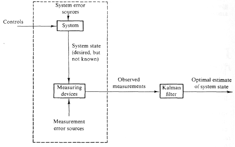
Figure 1.1 depicts a typical situation in which a Kalman ﬁlter could be used

advantageously. A system of some sort is driven by some known controls, and

measuring devices provide the value of certain pertinent quantities. Knowl-

edge of these system inputs and outputs is all that is explicitly available from

the physical system for estimation purposes.

The

need

for a ﬁlter now becomes apparent. Often the variables of interest,

some ﬁnite number of quantities to describe the “state” of the system, cannot

Maybeck, Peter S.,

Stochastic Models, Estimation, and Control

, Vol. 1 5

OPYRIGHT

CADEMIC

RESS

, I

ECEMBER

25, 1999 11:00

be measured directly, and some means of inferring these values from the avail-

able data must be generated. For instance, an air data system directly provides

static and pitot pressures, from which velocity must be inferred. This infer-

ence is complicated by the facts that the system is typically driven by inputs

other than our own known controls and that the relationships among the vari-

ous “state” variables and measured outputs are known only with some degree

of uncertainty. Furthermore, any measurement will be corrupted to some

degree by noise, biases, and device inaccuracies, and so a means of extracting

valuable information from a noisy signal must be provided as well. There may

also be a number of different measuring devices, each with its own particular

dynamics and error characteristics, that provide some information about a par-

ticular variable, and it would be desirable to combine their outputs in a sys-

tematic and optimal manner. A Kalman ﬁlter combines all available

measurement data, plus prior knowledge about the system and measuring

devices, to produce an estimate of the desired variables in such a manner that

the error is minimized statistically. In other words, if we were to run a number

of candidate ﬁlters many times for the same application, then the average

results of the Kalman ﬁlter would be better than the average results of any

other.

Conceptually, what any type of ﬁlter tries to do is obtain an “optimal” esti-

mate of desired quantities from data provided by a noisy environment, “opti-

mal” meaning that it minimizes errors in some respect. There are many means

of accomplishing this objective. If we adopt a Bayesian viewpoint, then we

want the ﬁlter to propagate the

conditional probability density

of the desired

FIG. 1. 1 Typical Kalman ﬁlter application

Maybeck, Peter S.,

Stochastic Models, Estimation, and Control

, Vol. 1 6

OPYRIGHT

CADEMIC

RESS

, I

ECEMBER

25, 1999 11:00

quantities, conditioned on knowledge of the actual data coming from the mea-

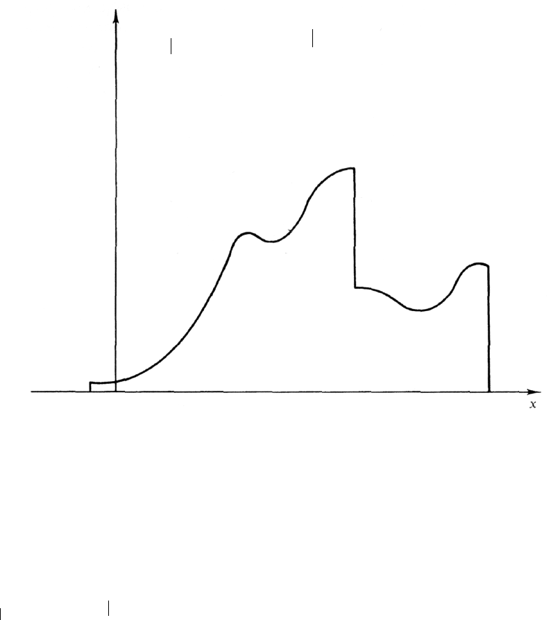
suring devices. To understand this concept, consider Fig. 1.2, a portrayal of a

conditional probability density of the value of a scalar quantity at time

instant ( ), conditioned on knowledge that the vector measurement at

time instant 1 took on the value ( ) and similarly for instants 2

through , plotted as a function of possible values. This is denoted as

. For example, let be the one-dimensional

position of a vehicle at time instant 1, and let be a two-dimensional vector

describing the measurements of position at time by two separate radars.

Such a conditional probability density contains all the available information

about : it indicates, for the given value of all measurements taken up

through time instant , what the probability would be of assuming any

particular value or range of values.

It is termed a “conditional” probability density because its shape and loca-

tion on the axis is dependent upon the values of the measurements taken. Its

shape conveys the amount of certainty you have in the knowledge of the value

of . If the density plot is a narrow peak, then most of the probability

“weight” is concentrated in a narrow band of values. On the other hand, if

the plot has a gradual shape, the probability “weight” is spread over a wider

range of , indicating that you are less sure of its value.

FIG. 1. 2 Conditional probability density.

fxi()z1()z2()…zi(),,, xz

1z2…zi

,,,()

ixi() z1()

z1z1() z1

ixi()

fxi()z1()z2()…zi(),,, xz

1z2…zi

,,,() xi()

zj()

xi()

ixi()

Maybeck, Peter S., Stochastic Models, Estimation, and Control, Vol. 1 7

Once such a conditional probability density function is propagated, the

“optimal” estimate can be deﬁned. Possible choices would include

(1) the mean—the “center of probability mass” estimate;

(2) the mode—the value of that has the highest probability, locating the

peak of the density; and

(3) the median—the value of such that half of the probability weight lies

to the left and half to the right of it.

A Kalman ﬁlter performs this conditional probability density propagation

for problems in which the system can be described through a linear model and

in which system and measurement noises are white and Gaussian (to be

explained shortly). Under these conditions, the mean, mode, median, and vir-

tually any reasonable choice for an “optimal” estimate all coincide, so there is

in fact a unique “best” estimate of the value of . Under these three restric-

tions, the Kalman ﬁlter can be shown to be the best ﬁlter of any conceivable

form. Some of the restrictions can be relaxed, yielding a qualiﬁed optimal ﬁl-

ter. For instance, if the Gaussian assumption is removed, the Kalman ﬁlter can

be shown to be the best (minimum error variance) ﬁlter out of the class of lin-

ear unbiased ﬁlters. However, these three assumptions can be justiﬁed for

many potential applications, as seen in the following section.

1.4 BASIC ASSUMPTIONS

At this point it is useful to look at the three basic assumptions in the Kal-

man ﬁlter formulation. On ﬁrst inspection, they may appear to be overly

restrictive and unrealistic. To allay any misgivings of this sort, this section

will brieﬂy discuss the physical implications of these assumptions.

A linear system model is justiﬁable for a number of reasons. Often such a

model is adequate for the purpose at hand, and when nonlinearities do exist,

the typical engineering approach is to linearize about some nominal point or

trajectory, achieving a perturbation model or error model. Linear systems are

desirable in that they are more easily manipulated with engineering tools, and

linear system (or differential equation) theory is much more complete and

practical than nonlinear. The fact is that there are means of extending the Kal-

man ﬁlter concept to some nonlinear applications or developing nonlinear ﬁl-

ters directly, but these are considered only if linear models prove inadequate.

“Whiteness” implies that the noise value is not correlated in time. Stated

more simply, if you know what the value of the noise is now, this knowledge

does you no good in predicting what its value will be at any other time. White-

ness also implies that the noise has equal power at all frequencies. Since this

results in a noise with inﬁnite power, a white noise obviously cannot really

exist. One might then ask, why even consider such a concept if it does not

Maybeck, Peter S., Stochastic Models, Estimation, and Control, Vol. 1 8

exist in real life? The answer is twofold. First, any physical system of interest

has a certain frequency “bandpass”—a frequency range of inputs to which it

can respond. Above this range, the input either has no effect, or the system so

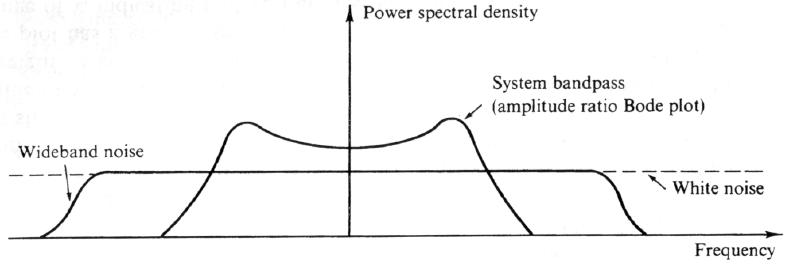
severely attenuates the effect that it essentially does not exist. In Fig. 1.3, a

typical system bandpass curve is drawn on a plot of “power spectral density”

(interpreted as the amount of power content at a certain frequency) versus fre-

quency. Typically a system will be driven by wideband noise—one having

power at frequencies above the system bandpass, and essentially constant

power at all frequencies within the system bandpass—as shown in the ﬁgure.

On this same plot, a white noise would merely extend this constant power

level out across all frequencies. Now, within the bandpass of the system of

interest, the ﬁctitious white noise looks identical to the real wideband noise.

So what has been gained? That is the second part of the answer to why a white

noise model is used. It turns out that the mathematics involved in the ﬁlter are

vastly simpliﬁed (in fact, made tractable) by replacing the real wideband noise

with a white noise which, from the system’s “point of view,” is identical.

Therefore, the white noise model is used.

One might argue that there are cases in which the noise power level is not

constant over all frequencies within the system bandpass, or in which the

noise is in fact time correlated. For such instances, a white noise put through a

small linear system can duplicate virtually any form of time-correlated noise.

This small system, called a “shaping ﬁlter,” is then added to the original sys-

tem, to achieve an overall linear system driven by white noise once again.

Whereas whiteness pertains to time or frequency relationships of a noise,

Gaussianness has to do with its amplitude. Thus, at any single point in time,

the probability density of a Gaussian noise amplitude takes on the shape of a

normal bell-shaped curve. This assumption can be justiﬁed physically by the

fact that a system or measurement noise is typically caused by a number of

small sources. It can be shown mathematically that when a number of inde-

pendent random variables are added together, the summed effect can be de-

scribed very closely by a Gaussian probability density, regardless of the shape

of the individual densities.

FIG. 1. 3 Power spectral density bandwidths.

Maybeck, Peter S., Stochastic Models, Estimation, and Control, Vol. 1 9

There is also a practical justiﬁcation for using Gaussian densities. Similar

to whiteness, it makes the mathematics tractable. But more than that, typically

an engineer will know, at best, the ﬁrst and second order statistics (mean and

variance or standard deviation) of a noise process. In the absence of any

higher order statistics, there is no better form to assume than the Gaussian

density. The ﬁrst and second order statistics completely determine a Gaussian

density, unlike most densities which require an endless number of orders of

statistics to specify their shape entirely. Thus, the Kalman ﬁlter, which propa-

gates the ﬁrst and second order statistics, includes all information contained

in the conditional probability density, rather than only some of it, as would be

the case with a different form of density.

The particular assumptions that are made are dictated by the objectives of,

and the underlying motivation for, the model being developed. If our objective

were merely to build good descriptive models, we would not conﬁne our atten-

tion to linear system models driven by white Gaussian noise. Rather, we

would seek the model, of whatever form, that best ﬁts the data generated by

the “real world.” It is our desire to build estimators and controllers based upon

our system models that drives us to these assumptions: other assumptions gen-

erally do not yield tractable estimation or control problem formulations. For-

tunately, the class of models that yields tractable mathematics also provides

adequate representations for many applications of interest. Later, the model

structure will be extended somewhat to enlarge the range of applicability, but

the requirement of model usefulness in subsequent estimator or controller

design will again be a dominant inﬂuence on the manner in which the exten-

sions are made.

1.5 A SIMPLE EXAMPLE

To see how a Kalman ﬁlter works, a simple example will now be developed.

Any example of a single measuring device providing data on a single variable

would sufﬁce, but the determination of a position is chosen because the proba-

bility of one’s exact location is a familiar concept that easily allows dynamics

to be incorporated into the problem.

Suppose that you are lost at sea during the night and have no idea at all of

your location. So you take a star sighting to establish your position (for the

sake of simplicity, consider a one-dimensional location). At some time you

determine your location to be . However, because of inherent measuring

device inaccuracies, human error, and the like, the result of your measurement

is somewhat uncertain. Say you decide that the precision is such that the stan-

dard deviation (one-sigma value) involved is (or equivalently, the variance,

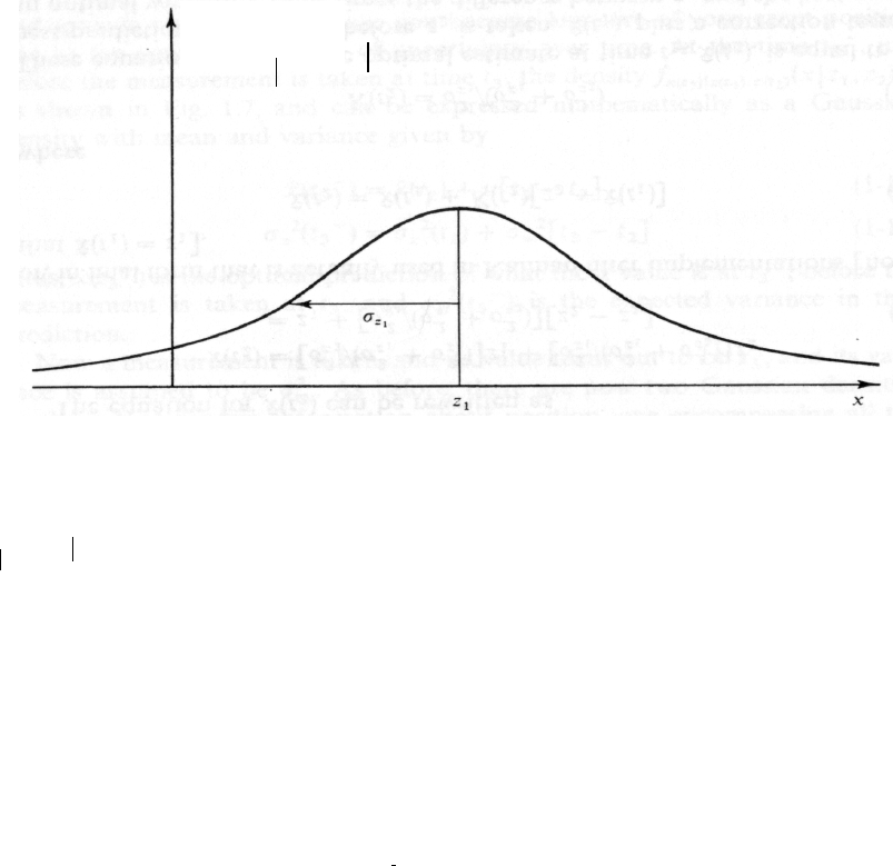
or second order statistic, is ,). Thus, you can establish the conditional prob-

ability of , your position at time , conditioned on the observed value of

σz1

() t1

Maybeck, Peter S., Stochastic Models, Estimation, and Control, Vol. 1 10

the measurement being , as depicted in Fig. 1.4. This is a plot of

as a function of the location : it tells you the probability of

being in any one location, based upon the measurement you took. Note that

is a direct measure of the uncertainty: the larger is, the broader the

probability peak is, spreading the probability “weight” over a larger range of

values. For a Gaussian density, 68.3% of the probability “weight” is con-

tained within the band units to each side of the mean, the shaded portion in

Fig. 1.4.

Based on this conditional probability density, the best estimate of your

position is

(1-1)

and the variance of the error in the estimate is

(1-2)

Note that is both the mode (peak) and the median (value with of the

probability weight to each side), as well as the mean (center of mass).

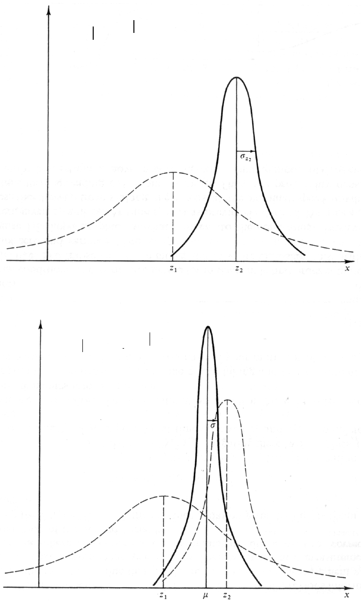
Now say a trained navigator friend takes an independent ﬁx right after you

do, at time (so that the true position has not changed at all), and obtains

a measurement with a variance . Because he has a higher skill, assume

the variance in his measurement to be somewhat smaller than in yours. Figure

1.5 presents the conditional density of your position at time , based only on

the measured value . Note the narrower peak due to smaller variance, indi-

cating that you are rather certain of your position based on his measurement.

At this point, you have two measurements available for estimating your

position. The question is, how do you combine these data? It will be shown

subsequently that, based on the assumptions made, the conditional density of

FIG. 1. 4 Conditional density of position based on measured value .z1

fxt

()zt

()

fxt

()zt

()

() x

σz1σz1

ˆt1

() z1

σx

2t1

() σ

ˆ12⁄

t2t1

≅

z2σz2

Maybeck, Peter S., Stochastic Models, Estimation, and Control, Vol. 1 11

FIG. 1. 5 Conditional density of position based on measurement alone.z2

FIG. 1. 6 Conditional density of position based on data and .z1z2

fxt

()zt

()

fxt

()zt

(),xz

1z2

,()

Maybeck, Peter S., Stochastic Models, Estimation, and Control, Vol. 1 12

your position at time , , given both and , is a Gaussian density

with mean and variance as indicated in Fig. 1.6, with

(1-3)

(1-4)

Note that, from (l-4), is less than either or , which is to say that the

uncertainty in your estimate of position has been decreased by combining the

two pieces of information.

Given this density, the best estimate is

(1-5)

with an associated error variance . It is the mode and the mean (or, since it

is the mean of a conditional density, it is also termed the conditional mean).

Furthermore, it is also the maximum likelihood estimate, the weighted least

squares estimate, and the linear estimate whose variance is less than that of

any other linear unbiased estimate. In other words, it is the “best” you can do

according to just about any reasonable criterion.

After some study, the form of given in Eq. (1-3) makes good sense. If

were equal to , which is to say you think the measurements are of equal

precision, the equation says the optimal estimate of position is simply the

average of the two measurements, as would be expected. On the other hand, if

were larger than , which is to say that the uncertainty involved in the

measurement is greater than that of , then the equation dictates “weight-

ing” more heavily than . Finally, the variance of the estimate is less than

, even if is very large: even poor quality data provide some information,

and should thus increase the precision of the ﬁlter output.

The equation for can be rewritten as

(1-6)

or, in ﬁnal form that is actually used in Kalman ﬁlter implementations [noting

that ]

(1-7)

where

(1-8)

These equations say that the optimal estimate at time , , is equal to the

best prediction of its value before is taken, , plus a correction term of

an optimal weighting value times the difference between and the best pre-

diction of its value before it is actually taken, . It is worthwhile to under-

stand this “predictor-corrector” structure of the ﬁlter. Based on all previous

t2t1

≅xt

() z1z2

µσ

2σz1

2σz2

+()⁄[]z1σz1

2σz1

2σz2

+()⁄[]z2

1σ2

⁄1σz1

⁄()1σz2

⁄()+=

σσ

z1σz2

ˆt2

() µ=

σ2

µσ

σz2

σz1σz2

z1z2

z2z1

σz1σz2

ˆt2

()

ˆt2

() σ

2σz1

2σz2

+()⁄[]z1σz1

2σz1

2σz2

+()⁄[]z2

z1σz1

2σz1

2σz2

+()⁄[]z2z1

–[]+=

ˆt1

() z1

ˆt2

() x

ˆt1

() Kt

()z2x

ˆt1

()–[]+=

() σ

2σz1

2σz2

+()⁄=

t2x

ˆt2

()

ˆt1

()

ˆt1

()

Maybeck, Peter S., Stochastic Models, Estimation, and Control, Vol. 1 13

information, a prediction of the value that the desired variables and measure-

ment will have at the next measurement time is made. Then, when the next

measurement is taken, the difference between it and its predicted value is used

to “correct” the prediction of the desired variables.

Using the in Eq. (l-8), the variance equation given by Eq. (1-4) can be

rewritten as

(1-9)

Note that the values of and embody all of the information in

. Stated differently, by propagating these two variables, the

conditional density of your position at time , given and , is completely

speciﬁed.

Thus we have solved the static estimation problem. Now consider incorpo-

rating dynamics into the problem.

Suppose that you travel for some time before taking another measurement.

Further assume that the best mode1 you have of your motion is of the simple

form

(1-10)

where is a nominal velocity and is a noise term used to represent the un-

certainty in your knowledge of the actual velocity due to disturbances, off-

nominal conditions, effects not accounted for in the simple ﬁrst order equa-

tion, and the like. The “noise” will be modeled as a white Gaussian noise

with a mean of zero and variance of .

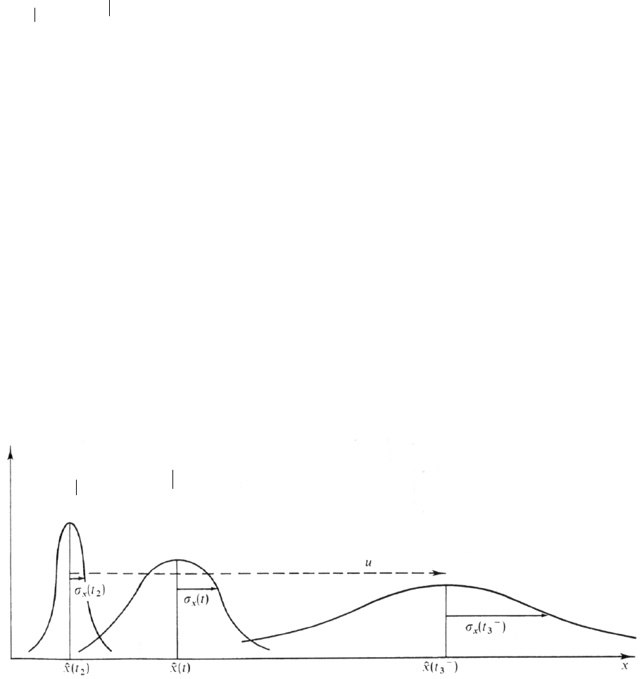
Figure 1.7 shows graphically what happens to the-conditional density of

position, given and . At time it is as previously derived. As time

progresses, the density travels along the axis at the nominal speed , while

simultaneously spreading out about its mean. Thus, the probability density

starts at the best estimate, moves according to the nominal model of dynamics,

()

σx

2t2

() σ

2t1

() Kt

()σ

2t1

()–=

ˆt2

() σ

2t2

()

fxt

()zt

(),xz

1z2

,()

t2z1z2

dx dt⁄uw+=

σw

FIG. 1. 7 Propagation of conditional probability density.

fxt()zt

()zt

(),xz

1z2

,()

z1z2t2

Maybeck, Peter S., Stochastic Models, Estimation, and Control, Vol. 1 14

and spreads out in time because you become less sure of your exact position

due to the constant addition of uncertainty over time. At the time , just

before the measurement is taken at time , the density is

as shown in Fig. 1.7, and can be expressed mathematically as a Gaussian den-

sity with mean and variance given by

(1-11)

(1-12)

Thus, is the optimal prediction of what the value is at , before the

measurement is taken at , and is the expected variance in that

prediction.

Now a measurement is taken, and its value turns out to be , and its vari-

ance is assumed to be . As before, there are now two Gaussian densities

available that contain information about position, one encompassing all the

information available before the measurement, and the other being the infor-

mation provided by the measurement itself. By the same process as before, the

density with mean and variance is combined with the density

with mean and variance to yield a Gaussian density with mean

(1-13)

and variance

(1-14)

where the gain is given by

(1-15)

The optimal estimate, , satisﬁes the same form of equation as seen previ-

ously in (1-7). The best prediction of its value before is taken is corrected

by an optimal weighting value times the difference between and the predic-

tion of its value. Similarly, the variance and gain equations are of the same

form as (1-8) and (1-9).

Observe the form of the equation for . If , the measurement noise

variance, is large, then is small; this simply says that you would tend to

put little conﬁdence in a very noisy measurement and so would weight it

lightly. In the limit as , becomes zero, and equals ; an

inﬁnitely noisy measurement is totally ignored. If the dynamic system noise

variance is large, then will be large [see Eq. (l-12)] and so will

; in this case, you are not very certain of the output of the system mode1

within the ﬁlter structure and therefore would weight the measurement

heavily. Note that in the limit as , and , so Eq. (1-

13) yields

(1-16)

—

fxt

()zt

(),xz

1z2

,()

ˆt3

—

() x

ˆt2

() ut

3t2

–[]+=

σx

2t3

—

() σ

2t2

() σ

2t3t2

–[]+=

ˆt3

—

() xt

—

t3σx

2t3

—

()

σz3

ˆt3

—

() σ

2t3

—

()

z3σz3

ˆt3

() x

ˆt3

—

()Kt

()z3x

ˆt3

—

()–[]+=

σx

2t3

() σ

2t3

—

()Kt

()σ

2t3

—

()–=

()

() σ

2t3

—

()σ

2t3

—

()σ

+[]⁄=

ˆt3

()

() σ

()

σz3

2∞→ Kt

() x

ˆt3

() x

ˆt3

—

()

σw

2σx

2t3

—

()

σw

2∞→σ

2t3

—

() ∞→Kt

() 1→

ˆt3

() x

ˆt3

—

()1z3x

ˆt3

—

()–[]⋅+= z3

Maybeck, Peter S., Stochastic Models, Estimation, and Control, Vol. 1 15

Thus in the limit of absolutely no conﬁdence in the system model output, the

optimal policy is to ignore the output and use the new measurement as the

optimal estimate. Finally, if should ever become zero, then so does

; this is sensible since if , you are absolutely sure of your esti-

mate before becomes available and therefore can disregard the measure-

ment.

Although we have not as yet derived these results mathematically, we have

been able to demonstrate the reasonableness of the ﬁlter structure.

1.6 A PREVIEW

Extending Eqs. (1-11) and (1-12) to the vector case and allowing time vary-

ing parameters in the system and noise descriptions yields the general Kalman

ﬁlter algorithm for propagating the conditional density and optimal estimate

from one measurement sample time to the next. Similarly, the Kalman ﬁlter

update at a measurement time is just the extension of Eqs. (l-13)-(1-15). Fur-

ther logical extensions would include estimation with data beyond the time

when variables are to be estimated, estimation with nonlinear system models

rather than linear, control of systems described through stochastic models, and

both estimation and control when the noise and system parameters are not

known with absolute certainty. The sequel provides a thorough investigation

of those topics, developing both the theoretical mathematical aspects and

practical engineering insights necessary to resolve the problem formulations

and solutions fully.

GENERAL REFERENCES

1. Aoki, M., Optimization of Stochastic Systems—Topics in Discrete-Time Systems. Academic

Press, New York, 1967.

2. Aström. K. J., Introduction to Stochastic Control Theory. Academic Press, New York, 1970.

3. Bryson, A. E. Jr., and Ho. Y., Applied Optimal Control. Blaisdell, Wahham, Massachusetts,

1969.

4. Bucy, R. S., and Joseph, P. D., Filtering for Stochastic Processes with Applications to Guidance.

Wiley, New York, 1968.

5. Deutsch, R., Estimation Theory. Prentice-Hall, Englewood Cliffs, New Jersey, 1965.

6. Deyst, J. J., “Estimation and Control of Stochastic Processes,” unpublished course notes. M.I.T.

Dept. of Aeronautics and Astronautics, Cambridge, Massachusetts, 1970.

7. Gelb, A. (ed.), Applied Optimal Estimation. M.I.T. Press, Cambridge, Massachusetts, 1974.

8. Jazwinski, A. H., Stochastic Processes and Filtering Theory. Academic Press, New York, 1970.

9. Kwakernaak. H., and Sivan. R., Linear Optimal Control Systems. Wiley, New York, 1972.

10. Lee, R. C. K., Optimal Estimation, Identiﬁcation and Control. M. I. T. Press, Cambridge, Mas-

sachusetts, 1964.

11. Liebelt, P. B., An Introduction to Optimal Estimation. Addison-Wesley, Reading, Massachusetts,

1967.

12. Maybeck, P. S., “The Kalman Filter—An Introduction for Potential Users,” TM-72-3, Air Force

Flight Dynamics Laboratory, Wright-Patterson AFB, Ohio, June 1972.

σx

2t3

—

()

() σ

2t3

—

() 0=

Maybeck, Peter S., Stochastic Models, Estimation, and Control, Vol. 1 16

13. Maybeck, P. S., “Applied Optimal Estimation—Kalman Filter Design and Implementation,”

notes for a continuing education course offered by the Air Force Institute of Technology,

Wright-Patterson AFB, Ohio, semiannually since December 1974.

14. Meditch, J. S., Stochastic Optimal Linear Estimation and Control. McGraw-Hill, New York,

1969.

15. McGarty, T. P., Stochastic Systems and State Estimation. Wiley, New York, 1974.

16. Sage, A. P., and Melsa, J. L., Estimation Theory with Application to Communications and Con-

trol. McGraw-Hill, New York, 1971.

17. Schweppe, F. C., Uncertain Dynamic Systems. Prentice-Hall, Englewood Cliffs, New Jersey,

1973.

18. Van Trees, H. L., Detection, Estimation and Modulation Theory, Vol. 1. Wiley, New York, 1968.

Maybeck_ch1_10 Maybeck_ch1 Maybeck Ch1

Navigation menu

Versions of this User Manual:

Views

Navigation