Mc 105
User Manual: MC 105
Open the PDF directly: View PDF ![]() .
.
Page Count: 385 [warning: Documents this large are best viewed by clicking the View PDF Link!]

1
MANAGEMENT ACCOUNTING: NATURE AND SCOPE
Objective: The present lesson explains the meaning, nature, scope and limitations
of accounting. Further, it discusses the activities covered under
management accounting and its difference with financial accounting.
LESSON STRUCTURE
1.1 Introduction
1.2 Definitions of Management Accounting
1.3 Nature of Management Accounting
1.4 Functions of Management Accounting
1.5 Scope of Management Accounting
1.6 The Management Accountant
1.7 Management Accounting and Financial Accounting
1.8 Cost Accounting and Management Accounting
1.9 Limitations of Management Accounting
1.10 Self-Test Questions
1.11 Suggested Readings
1.1 INTRODUCTION
Management accounting can be viewed as Management-oriented Accounting.
Basically it is the study of managerial aspect of financial accounting,
"accounting in relation to management function". It shows how the accounting
function can be re-oriented so as to fit it within the framework of management
activity. The primary task of management accounting is, therefore, to
redesign the entire accounting system so that it may serve the operational
COURSE: MANAGEMENT ACCOUNTING
COURSE CODE: MC-105 AUTHOR: Dr. N. S. MALIK
LESSON: 01
V
ETTER: Prof. M S Turan
2
needs of the firm. If furnishes definite accounting information, past, present or
future, which may be used as a basis for management action. The financial
data are so devised and systematically development that they become a
unique tool for management decision.
1.2 DEFINITIONS OF MANAGEMENT ACCOUNTING
The term “Management Accounting”, observe, Broad and Carmichael, covers
all those services by which the accounting department can assist the top
management and other departments in the formation of policy, control of
execution and appreciation of effectiveness. This definition points out that
management is entrusted with the primary task of planning, execution and
control of the operating activities of an enterprise. It constantly needs
accounting information on which to base its decision. A decision based on
data is usually correct and the risk of erring is minimized. The position of the
management in respect of its functions can be compared to that of an army
general who wants to wage a successful battle. A general can hardly fight
successfully unless he gets full information about the surrounding situation
and the extent of effectiveness of each of his battalions and, to the extend
possible, even the enemy's intentions. Like a general a successful
management too strives to outstrip other competitors in the field by
streamlining its operating efficiency. It needs a thorough knowledge of the
situation and the circumstances in which the firm operates. Such knowledge
can only be gained through the processed financial data rendered by the
accounting department on the basis of which it can take policy decision
regarding execution, control, etc. It is here that the role of management
accounting comes in. It supplies all sorts of accounting information in the
3
form of such statements as may be needed by the management. Therefore,
management accounting is concerned with the accumulation, classification
and interpretation of information that assists individual executives to fulfill
organizational objectives.
The Report of the Anglo-American Council of Productivity (1950) has also
given a definition of management accounting, which has been widely
accepted. According to it, "Management accounting is the presentation of
accounting information in such a way as to assist the management in creation
of policy and the day to day operation of an undertaking". The reasoning
added to this statement was, "the technique of accounting is of extreme
importance because it works in the most nearly universal medium available
for the expression of facts, so that facts of great diversity can be represented
in the same picture. It is not the production of these pictures that is a function
of management but the use of them." An analysis of the above definition
shows that management needs information for better decision-making and
effectiveness. The collection and presentation of such information come
within the area of management accounting. Thus, accounting information
should be recorded and presented in the form of reports at such frequent
intervals, as the management may want. These reports present a systematic
review of past events as well as an analytical survey of current economic
trends. Such reports are mainly suggestive in approach and the data
contained in them are quite up to date. The accounting data so supplied thus
provide the informational basis of action. The quality of information so
supplied depends upon its usefulness to management in decision-making.
The usual approach is that, first of all, a thorough analysis of the whole
4
managerial process is made, then the information required for each area is
explored, and finally, all the information, after analysis in terms of alternatives,
is taken into consideration before arriving at a management decision. It is to
be understood here that the accounting information has no end in itself; it is a
means to an end. As its basic idea is to serve the management, its form and
frequency are all decided by managerial needs. Therefore, accounting aids
the management by providing quantitative information on the economic well
being of the enterprise. It would be appropriate if we called management
accounting an Enterprise Economics. Its scope extends to the use of certain
modern sophisticated managerial techniques in analyzing and interpreting
operative data and to the establishment of a communication network for
financial reporting at all managerial levels of an organization.
1.3 NATURE OF MANAGEMENT ACCOUNTING
The term management accounting is composed of 'management' and
'accounting'. The word 'management' here does not signify only the top
management but the entire personnel charged with the authority and
responsibility of operating an enterprise. The task of management accounting
involves furnishing accounting information to the management, which may
base its decisions on it. It is through management accounting that the
management gets the tools for an analysis of its administrative action and can
lay suitable stress on the possible alternatives in terms of costs, prices and
profits, etc. but it should be understood that the accounting information
supplied to management is not the sole basis for managerial decisions. Along
with the accounting information, management takes into consideration or
weighs other factors concerning actual execution. For reaching a final
5
decision, management has to apply its common sense, foresight, knowledge
and experience of operating an enterprise, in addition to the information that is
already has.
The word 'accounting' used in this phrase should not lead us to believe that it
is restricted to a mere record of business transactions i.e., book keeping only.
It has indeed a 'macro-economic approach'. As it draws its raw material from
several other disciplines like costing, statistics, mathematics, financial
accounting, etc., it can be called an interdisciplinary subject, the scope of
which is not clearly demarcated. Other fields of study, which can be covered
by management accounting, are political science, sociology, psychology,
management, economics, statistics, law, etc. A knowledge of political science
helps to understand authority relationship and responsibility identification in an
organization. A study of sociology helps to understand the behaviour of man
in groups. Psychology enables us to know the mental make-up of employers
and employees. A knowledge of these subjects helps to increase motivation,
and to control the actions of the people who are ultimately responsible for
costs. This builds a better employer-employee relationship and a sound
morale. The subject of management reveals the processes involved in the art
of managing, a knowledge of economics assists in the determination of
optimum output in the forecasting of sales and production, etc., and also
makes it possible to analyze management action in terms of cost revenues,
profits, growth, etc. It is with the help of statistics that this information is
presented to the management in a form that can be assimilated. The subject
of management accounting also encompasses the subject of law, knowledge
6
of which is necessary to find out if the management action is ultra-vires or not.
It is, therefore, a wide and diverse subject.
Management accounting has no set principles such as the double entry
system of bookkeeping. In place of generally accepted accounting principles,
the philosophy of cost benefit analysis is the core guide of this discipline. It
says that no accounting system is good or bad but is can be considered
desirable so long as it brings incremental benefits in excess of its incremental
costs. Applying management accounting principles to financial matters can
arrive at no single perfect solution. It is, therefore, an inexact science, which
uses its own conventions rather than standardized principles. The facts to be
studied here can be interpreted in different ways and the precision of the
inferences depends upon the skill, judgement and common sense of different
management accountants. It occupies a middle position between a fully
matured and an infant subject.
Since management accounting is managerially oriented, its data is selective in
nature. It focuses on potential opportunities rather than opportunities lost.
The data is operative in nature catering to the operational needs of a firm. It
details events, monetary and non-monetary. The nature of data, the form of
presentation and its duration are mainly determined by managerial needs. It
is quite frequently reported as it is meant for internal uses and managerial
control. An accountant should look at his enterprise from the management's
point of view. Whenever he fails to do that he ceases to be a management
accountant.
Management accounting is highly sensitive to management needs. However,
it assists the management and does not replace it. It represents a service
7
phase of management rather than a service to management from
management accountant. It is rather highly personalized service. Finally, it
can be said that the management accounting serves as a management
information system and so enables the management to manage better.
1.4 FUNCTIONS OF MANAGEMENT ACCOUNTING
The basic function of management accounting is to assist the management in
performing its functions effectively. The functions of the management are
planning, organizing, directing and controlling. Management accounting helps
in the performance of each of these functions in the following ways:
(i) Provides data: Management accounting serves as a vital source of
data for management planning. The accounts and documents are a
repository of a vast quantity of data about the past progress of the
enterprise, which are a must for making forecasts for the future.
(ii) Modifies data: The accounting data required for managerial decisions
is properly compiled and classified. For example, purchase figures for
different months may be classified to know total purchases made
during each period product-wise, supplier-wise and territory-wise.
(iii) Analyses and interprets data: The accounting data is analyzed
meaningfully for effective planning and decision-making. For this
purpose the data is presented in a comparative form. Ratios are
calculated and likely trends are projected.
(iv) Serves as a means of communicating: Management accounting
provides a means of communicating management plans upward,
downward and outward through the organization. Initially, it means
identifying the feasibility and consistency of the various segments of
8
the plan. At later stages it keeps all parties informed about the plans
that have been agreed upon and their roles in these plans.
(v) Facilitates control: Management accounting helps in translating
given objectives and strategy into specified goals for attainment by a
specified time and secures effective accomplishment of these goals in
an efficient manner. All this is made possible through budgetary
control and standard costing which is an integral part of management
accounting.
(vi) Uses also qualitative information: Management accounting does
not restrict itself to financial data for helping the management in
decision making but also uses such information which may not be
capable of being measured in monetary terms. Such information may
be collected form special surveys, statistical compilations, engineering
records, etc.
1.5 SCOPE OF MANAGEMENT ACCOUNTING
Management accounting is concerned with presentation of accounting
information in the most useful way for the management. Its scope is,
therefore, quite vast and includes within its fold almost all aspects of business
operations. However, the following areas can rightly be identified as falling
within the ambit of management accounting:
(i) Financial Accounting: Management accounting is mainly concerned
with the rearrangement of the information provided by financial
accounting. Hence, management cannot obtain full control and
coordination of operations without a properly designed financial
accounting system.
9
(ii) Cost Accounting: Standard costing, marginal costing, opportunity
cost analysis, differential costing and other cost techniques play a
useful role in operation and control of the business undertaking.
(iii) Revaluation Accounting: This is concerned with ensuring that capital
is maintained intact in real terms and profit is calculated with this fact in
mind.
(iv) Budgetary Control: This includes framing of budgets, comparison of
actual performance with the budgeted performance, computation of
variances, finding of their causes, etc.
(v) Inventory Control: It includes control over inventory from the time it is
acquired till its final disposal.
(vi) Statistical Methods: Graphs, charts, pictorial presentation, index
numbers and other statistical methods make the information more
impressive and intelligible.
(vii) Interim Reporting: This includes preparation of monthly, quarterly,
half-yearly income statements and the related reports, cash flow and
funds flow statements, scrap reports, etc.
(viii) Taxation: This includes computation of income in accordance with the
tax laws, filing of returns and making tax payments.
(ix) Office Services: This includes maintenance of proper data processing
and other office management services, reporting on best use of
mechanical and electronic devices.
(x) Internal Audit: Development of a suitable internal audit system for
internal control.
(xi)
10
1.6 THE MANAGEMENT ACCOUNTANT
Management Accounting provides significant economic and financial data to
the management and the Management Accountant is the channel through
which this information efficiently and effectively flows to the management. The
Management Accountant has a very significant role to perform in the
installation, development and functioning of an efficient and effective
management information system. He designs the framework of the financial
and cost control reports that provide each management level with the most
useful data at the most appropriate time. He educates executives in the need
for control information and ways of using it. This is because his position is
unique with respect to information about the organization. Apart from top
management no one in the organization perhaps knows more about the
various functions of the organization than him. He is, therefore, sometimes
described as the Chief Intelligence Officer of the top management. He
gathers information, breaks it down, sifts it out and organizes it into
meaningful categories. He separates relevant and irrelevant information and
then ranks relevant information in an intelligible form to the management and
sometimes also to those who are interested in the information in the
information outside the company. He also compares the actual performance
with the planned one and reports and interprets the results of operations to all
levels of management and to the owners of the business. Thus, in brief,
management accountant or controller is the person who designs the
management information system for the organization, operates it by means of
interlocked budgets, computes variances and exhorts others to institute

11
corrective measures. Mr. P.L. Tandon has explained beautifully the position
of the management accountant in the following words.
"The management accountant is exactly like the spokes in a wheel,
connecting the rim of the wheel and the hub receiving the information. He
processes the information and then returns the processed information back to
where it came from"1.
Dr. Don barker2 sees a very bright future for the management accountants.
According to him, "Management Accountants will be presented with many
opportunities for innovative actions in the global economic environment. In
addition to their role of providing accurate, timely and relevant information,
management accountants will be expected to participate as business
consultants and partners with management in the strategic planning process".
Thus, there are tremendous possibilities for management accountants to
shine as a professional group in the years to come. To fit in this role, it is
necessary that the management accountants develop effective
communication abilities, adopt a structured approach, a flexible
accommodation and keep themselves aware with the latest evolving
technologies in the profession.
FUNCTIONS OF MANAGEMENT ACCOUNTANT
It is the duty of the management accountant to keep all levels of management
informed of their real position. He has, therefore, varied functions to perform.
His important functions can be summarized as follows:
1 Tandon, P.L.: "The Role of Management Accountants in General Management”. 4th All India
Seminar on Management Accounting, Lucknow, Feb. 1963.
2. President (1991-92), The Institute of Management Accountants, USA.
12
(i) Planning: He has to establish, coordinate and administer as an
integral part of management, an adequate plan for the control of the
operations. Such a plan would include profit planning, programmes of
capital investment and financing, sales forecasts, expenses budgets
and cost standards.
(ii) Controlling: He has to compare actual performance with operating
plans and standards and to report and interpret the results of
operations to all levels of management and the owners of the business.
This id done through the compilation of appropriate accounting and
statistical records and reports.
(iii) Coordinating: He consults all segments of management responsible
for policy or action. Such consultation might concern any phase of the
operation of the business having to do with attainment of objectives
and the effectiveness of the organizational structures and policies.
(iv) Other functions:
¾ He administers tax policies and procedures.
¾ He supervises and coordinated the preparation of reports to
governmental agencies.
¾ He ensures fiscal protection for the assets of the business through
adequate internal control and proper insurance coverage.
¾ He carries out continuous appraisal economic and social forces and
the government influences, and interprets their effect on the
business.
It should be noted that the functions of a Management Accountant are
more of those of a 'staff official'. He, in addition to processing historical
13
data, supplies a good deal of information concerning the future
operations in line with the management's needs. Besides serving top
management with information concerning the company as a whole, he
supplies detailed information to the line officers regarding alternative
plans and their profitability, which help them in decision-making. As a
matter of fact the Management Accountant should not bother himself
regarding the decision taken by the line officials after tendering advice
unless he has reasonable grounds to believe that such a decision is
going to affect the interests of corporation adversely. In such an event
also he should report it to the concerned level of management with
tact, firmness combined with politeness.
1.7 MANAGEMENT ACCOUNTING AND FINANCIAL ACCOUNTING
Financial accounting and management accounting are closely interrelated
since management accounting is to a large extent rearrangement of the data
provided by financial accounting. Moreover, all accounting is financial in the
sense that all accounting systems are in monetary terms and management is
responsible for the contents of the financial accounting statements. In spite of
such a close relationship between the two, there are certain fundamental
differences. These differences can be laid down as follows:
(i) Objectives: Financial accounting is designed to supply information in
the form of profit and loss account and balance sheet to external
parties like shareholders, creditors, banks, investors and Government.
Information is supplied periodically and is usually of such type in which
management is not much interested. Management Accounting is
designed principally for providing accounting information for internal
14
use of the management. Thus, financial accounting is primarily an
external reporting process while management accounting is primarily
an internal reporting process.
(ii) Analyzing performance: Financial accounting portrays the position of
business as a whole. The financial statements like income statement
and balance sheet report on overall performance or statues of the
business. On the other hand, management accounting directs its
attention to the various divisions, departments of the business and
reports about the profitability, performance, etc., of each of them.
Financial accounting deals with the aggregates and, therefore, cannot
reveal what part of the management action is going wrong and why.
Management accounting provides detailed analytical data for these
purposes.
(iii) Data used: Financial accounting is concerned with the monetary
record of past events. It is a post-mortem analysis of past activity and,
therefore, out the date for management action. Management
accounting is accounting for future and, therefore, it supplies data both
for present and future duly analyzed in detail in the 'management
language' so that it becomes a base for management action.
(iv) Monetary measurement: In financial accounting only such economic
events find place, which can be described in money. However, the
management is equally interested in non-monetary economic events,
viz., technical innovations, personnel in the organization, changes in
the value of money, etc. These events affect management's decision
and, therefore, management accounting cannot afford to ignore them.
15
For example, change in the value of money may not find a place in
financial accounting on account of "going concern concept". But while
affecting an insurance policy on an asset or providing for replacement
of an asset, the management will have to take into account this factor.
(v) Periodicity of reporting: The period of reporting is much longer in
financial accounting as compared to management accounting. The
Income Statement and the Balance Sheet are usually prepared yearly
or in some cases half-yearly. Management requires information at
frequent intervals and, therefore, financial accounting fails to cater to
the needs of the management. In management accounting there is
more emphasis on furnishing information quickly and at comparatively
short intervals as per the requirements of the management.
(vi) Precision: There is less emphasis on precision in case of
management accounting as compared to financial accounting since the
information is meant for internal consumption.
(vii) Nature: Financial accounting is more objective while management
accounting is more subjective. This is because management
accounting is fundamentally based on judgement rather than on
measurement.
(viii) Legal compulsion: Financial accounting has more or less become
compulsory for every business on account of the legal provisions of
one or the other Act. However, a business is free to install or not to
install system of management accounting.
The above points of difference between Financial Accounting and
Management Accounting prove that Management Accounting has flexible

16
approach as compared to rigid approach in the case of Financial Accounting.
In brief, financial accounting simply shows how the business has moved in the
past while management accounting shows how the business has to move in
the future.
An attempt may now be made to compare and study the two types of
accounting on basis of the characteristics of the data used. It is presented
through the box- 1.1, given below.
Box 1.1
Features of data Provided by Financial Provided by
Accounting Management accounting
1. Period After a stated period At frequent intervals
2. Time Historical data Current and future data
3. Unit of expression Money only Any statistical unit
4. Nature Actual data Projected data
5. Specificity Aggregates Detailed analysis
6. Description Money consequences Events
7. Reality Objective Subjective
8. Precision Pie to Pie accuracy May be guess-work
9. Principles Double entry system Cost benefit analysis
10. Legality Obligatory Optional
11. Purpose Overview of entire Analytical details of such
Business activity activities as call for decisions
1.8 COST ACCOUNTING AND MANAGEMENT ACCOUNTING
Cost accounting is the process of accounting for costs. It embraces the
accounting procedures relating to recording of all income and expenditure and
the preparation of periodical statements and reports with the object of
ascertaining and controlling costs. It is, thus, the formal mechanism by
means of which the costs of products or services are ascertained and
controlled. On the other hand, management accounting involves collecting,
analyzing, interpreting and presenting all accounting information, which is
useful to the management. It is closely associated with management control,
which comprises planning, executing, measuring and evaluating the
17
performance of an organization. Thus, management accounting draws
heavily on cost data and other information derived from cost accounting.
Today cost accounting is generally indistinguishable from the so-called
management accounting or internal accounting because it serves multiple
purposes. However, management accounting can be distinguished from cost
accounting in one important respect. Management accounting has a wider
scope as compared to cost accounting. Cost accounting deals primarily with
cost data while management accounting involves the considerations of both
cost and revenue. Management accounting is an all inclusive accounting
information system, which covers financial accounting, cost accounting, and
all aspects of financial management. But it is not a substitute for other
accounting functions. It involves a continuous process of reporting cost,
financial and other relevant data in an analytical and informative way to
management. We should not be very much concerned with boundaries of cost
accounting and management accounting since they are complementary in
nature. In the absence of a suitable system of cost accounting, management
accountant will not be in a position to have detailed cost information and his
function is bound to lose significance. On the other hand, the management
accountant cannot effectively use the cost data unless it has been reported to
him in a meaningful and informative form.
1.9 LIMITATIONS OF MANAGEMENT ACCOUNTING
Management accounting, being comparatively a new discipline, suffers from
certain limitations, which limit its effectiveness. These limitations are as
follows:
18
1. Limitations of basic records: Management accounting derives its
information from financial accounting, cost accounting and other
records. The strength and weakness of the management accounting,
therefore, depends upon the strength and weakness of these basic
records. In other words, their limitations are also the limitations of
management accounting.
2. Persistent efforts. The conclusions draws by the management
accountant are not executed automatically. He has to convince people
at all levels. In other words, he must be an efficient salesman in selling
his ideas.
3. Management accounting is only a tool: Management accounting
cannot replace the management. Management accountant is only an
adviser to the management. The decision regarding implementing his
advice is to be taken by the management. There is always a
temptation to take an easy course of arriving at decision by intuition
rather than going by the advice of the management accountant.
4. Wide scope: Management accounting has a very wide scope
incorporating many disciplines. It considers both monetary as well as
non-monetary factors. This all brings inexactness and subjectivity in
the conclusions obtained through it.
5. Top-heavy structure: The installation of management accounting
system requires heavy costs on account of an elaborate organization
and numerous rules and regulations. It can, therefore, be adopted only
by big concerns.
19
6. Opposition to change: Management accounting demands a break
away from traditional accounting practices. It calls for a rearrangement
of the personnel and their activities, which is generally not like by the
people involved.
7. Evolutionary stage: Management accounting is still in its initial stage.
It has, therefore, the same impediments as a new discipline will have,
e.g., fluidity of concepts, raw techniques and imperfect analytical tools.
This all creates doubt about the very utility of management accounting.
1.10 SELF-TEST QUESTIONS
1. What do you mean by management accounting? Explain giving examples.
2. What are the functions of a management accountant? Elaborate each one
of them.
3. Explain the benefits of management accounting in the business sector and
service sector.
4. Distinguish management accounting from financial accounting and cost
accounting.
5. Explain the limitations of management accounting.
1.11 SUGGESTED READINGS
1. Ashish K. Bhattacharya, Principles and Practices of Cost Accounting
(3rd.), New Delhi: Prentice Hall of India Private Limited, 2004.
2. Charles T. Horngren, Cost Accounting, A Managerial Emphasis,
Prentice Hall Inc., 1973.
3. D. T. Decoster and E. L. Schafer, Management Accounting, New York:
John Willey and Sons, 1979.
4. John G. Blocker and Wettmer W. Keith, Cost Accounting, New Delhi:
Tata Mc Grw Publishing Co. Ltd., 1976.
5. R. K. Sharma and Shashi K. Gupta, Management Accounting-
Principles and Practice (7th.), New Delhi: Kalyani Publishers, 1996.

20
FINANCIAL STATEMENT ANALYSIS
Objective: The present lesson explains the discrepancy between accounting
income and economic income; identify the devices used in practice to
exploit the use of the bottom line; the use of a firm's financial
statements to calculate standard financial ratios; decompose the return
on equity into its key determinants; carry out comparative analysis; and
highlights the uses of financial statement analysis for different
purposes.
LESSON STRUCTURE
2.1 Introduction
2.2 Financial Statements
2.3 Financial Statement Analysis
2.4 Methodical Presentation of Financial Statement Analysis
2.5 Techniques /Tools of Financial Statement Analysis
2.6 Self-Test Questions
2.7 Suggested Readings
2.1 INTRODUCTION
Financial statements are an important source of information for evaluating the
performance and prospects of a firm. If properly analyzed and interpreted,
financial statements can provide valuable insights into a firm's performance.
Analysis of financial statements is of interest to lenders (short term as well as
long term), investors, security analysts, managers, and others. Financial
statement analysis may be done for a variety of purposes, which may range
COURSE: MANAGEMENT ACCOUNTING
COURSE CODE: MC-105 AUTHOR: DR. N. S. MALIK
LESSON: 02
V
ETTER: Dr. Karam Pal
21
from a simple analysis of the short-term liquidity position of the firm to a
comprehensive assessment of the strengths and weaknesses of the firm in
various areas. It is helpful in assessing corporate excellence, judging
creditworthiness, forecasting bond ratings, evaluating intrinsic value of equity
shares, predicting bankruptcy, and assessing market risk.
2.2 FINANCIAL STATEMENTS
Managers, shareholders, creditors and other interested groups seek answers
to the following questions about a firm: What is the financial position of firm at
a given point of time? How has the firm performed financially over a given
period of time? What have been the sources and uses of cash over a given
period? To answer these questions, the accountant prepares two principal
statements, the balance sheet and the profit and loss account, and an
ancillary statement, the cash flow statement.
2.2.1 BALANCE SHEET
The balance sheet shows the financial condition of a business at a given point
of time. As per the Companies Act, the balance sheet of a company shall be
in either the account (horizontal) form or the report (vertical) form. Exhibit 2.1
shows the balance sheet of Horizon Limited as on March 31, 2005 cast in the
account as well as the report form. While the report form is most commonly
used by companies, it is more convenient to explain the contents of the
balance sheet of Horizon Limited, cast in the account form, as given Exhibit
2.2.
Structure of Balance Sheet as per the Companies Act
Exhibit 2.1 Account Form

22
Liabilities Assets
Share capital Fixed assets
Reserves and surplus Investments
Unsecured loans Current assets, loans and
advances
Current liabilities and provisions Current assets
Current liabilities Loans and advances
Provisions Miscellaneous expenditure
and losses
Exhibit 2.2 Report Form
I Sources of Funds
(1) Shareholders funds
(a) Share capital
(b) Reserves & surplus
(2) Loan funds
(a) Secured loans
(b) Unsecured loans
II Application of Funds
(1) Fixed assets
(2) Investments
(3) Current assets, loans and advances
Less: Current liabilities and provisions
Net current assets
(4) Miscellaneous expenditure and losses.
Liabilities. Liabilities defined very broadly represent what the business entity
owes others. The Companies Act classifies them as share capital, reserves
and surplus, secured loans, unsecured loans, current liabilities and provisions
Share Capital: This is divided into two types: equity capital and preference
capital. The first represents the contribution of equity shareholders who are
the owners to the firm. Equity capital, being risk capital, carries no fixed rate
of dividend. Preference capital represents the contribution of preference
shareholders and the dividend rate payable on it is fixed.
23
Reserves and Surplus: Reserves and surplus are profits, which have been
retained in the firm. There are two types of reserves: revenue reserves and
capital reserves. Revenue reserves represent accumulated retained earning
from the profits of normal business operations. These are held in various
forms: general reserve, investment allowance reserve, capital redemption
reserves, dividend equalization reserve, and so on. Capital reserves arise out
gains, which are not related to normal business operations. Examples of such
gains are the premium on issue of shares or gain on revaluation of assets.
Surplus is the balance in the profit and loss account, which has not been
appropriated to any particular reserve account. Note that reserves and
surplus along with equity capital represent owners' equity or net worth.
Secured Loans: These are the borrowings of the firm against which specific
collateral have been provided. The important components of secured loans
are: debentures, loans from financial institutions, and loans from commercial
banks.
Unsecured Loans. These are the borrowing of the firm against which no
specific security has been provided. The major components of unsecured
loans are: fixed deposits, loans and advances from promoters, inter-corporate
borrowings, and unsecured loans from banks.
Current liabilities and Provisions: Current liabilities and provisions, as per
the classification under the companies Act, consist of the amounts due to the
suppliers of goods and services bought on credit, advance payments
received, accrued expenses, unclaimed dividend, provisions for taxes,
dividends, and so on. Current liabilities for managerial purposes (as distinct
from their definition in the Companies Act) are obligations, which are expected
24
to mature in the next twelve months. So defined, they include current
liabilities and provisions as per the classification under the Companies Act
plus loans (secured and unsecured) which are repayable within one year from
the date of the balance sheet.
Assets: Broadly speaking, assets represent resources, which are of some
value to the firm. They have been acquired at a specific monetary cost by the
firm for the conduct of its operations. Assets are classified under the
Companies Act as fixed assets, investments, current assets, loans and
advances, miscellaneous expenditure and losses.
Fixed Assets: These assets have two characteristics: they are acquired for
use over relatively long periods for carrying on the operations of the firm and
they are ordinarily not meant for resale. Examples of fixed assets are land,
buildings, plant, machinery, patents, and copyrights.
Investments: These are financial securities owned by the firm. Some
investments represent long-term commitment of funds (usually these are the
equity shares of other firms held for income and control purposes). Other
investments are likely to be short term in nature such as holdings of units in
mutual fund schemes and may rightly be classified under current assets for
managerial purposes. (Under the requirements of the Companies Act,
however, short term holding of financial securities also has to be shown under
investments and not under current assets.)
Current Assets, Loans and Advances: This category consists of cash and
other assets, which get converted into cash during the operating cycle of the
fir. Current assets are held for a short period of time as against fixed assets,
which are held for relatively longer periods. The major components of current
25
assets are: cash, sundry debtors, inventories, loans and advances, and pre-
paid expenses. Cash denotes funds readily disbursable by the firm. The bulk
of it is usually in the form of bank balances and the rest is currency held by
the fir. Sundry debtors (also called accounts receivable) represent the
amounts owned to the firm by its customers who have bought goods and
services on credit. Sundry debtors are shown in the balance sheet at the
amount owed, less an allowance for bad debts. Inventories (also called
stocks) consist of raw materials, work-in-process, finished goods, and stores
and spares. They are usually reported at the lower of the cost or market
value. Loans and advances are the amounts loaned to employees, advances
given to suppliers and contractors, advance tax paid, and deposits made with
governmental and other agencies. They are shown at the actual amount.
Pre-paid expenses are expenditures incurred for services to be rendered in
the future. These are shown at the cost unexpired service.
Miscellaneous Expenditures and Losses: This category consists of two
items: (i) miscellaneous expenditures and (ii) losses. Miscellaneous
expenditures represent certain outlays such as preliminary expenses and
developmental expenses, which have not been written off. From the
accounting point of view, a loss represents a decrease in owners' equity.
Hence, when a loss occurs, the owners' equity should be reduced by that
amount. However, as per company law requirements, the share capital
(representing owners' equity) cannot be reduced when a loss occurs. So the
share capital is kept intact on the left hand side (the liabilities side) of the
balance sheet and the loss is shown on the right hand side (the assets side)
of the balance sheet.
26
2.2.2 PROFIT AND LOSS ACCOUNT
The Companies Act has prescribed a standard form for the balance sheet, but
none for the profit and loss account. However, the Companies Act does
require that the information provided should be adequate to reflect a true and
fair picture of the operations of the company for the accounting period. The
Companies Act has also specified that the profit and loss account must show
specific information as required by Schedule IV. The profit and loss account,
like the balance sheet, may be presented in the account form or the report
form. Typically, companies employ the report form. The report form
statement may be a single-step statement or a multi-step statement. In a
single step statement, all revenue items are recorded first, then the expense
items are show and finally the net profit is given. While a single step profit and
loss account aggregates all revenues and expenses, a multi-step profit and
loss account provides disaggregated information. Further, instead of showing
only the final profit measure, viz., the profit after tax figure, it presents profit
measures at intermediate stages as well.
¾ Net sales
¾ Cost of goods sold
¾ Gross profit
¾ Operating expenses
¾ Operating profit
¾ Non-operating surplus/deficit
¾ Profit before interest and tax
¾ Interest
¾ Profit before tax
¾ Tax
¾ Profit after tax.
2.3 FINANCIAL STATEMENTS ANALYSIS

27
Financial Statements Analysis (FSA) refers to the process of the critical
examination of the financial information contained in the financial statements in order
to understand and make decisions regarding the operations of the firm. The FSA is
basically a study of the relationship among various financial facts and figures is given
in a set of financial statements. The basic financial statements i.e. the Balance Sheet
and the Income Statement, already discussed in the preceding lesson contain a whole
lot of historical data. The complex figures as given in these financial statements are
dissected/broken up into simple and valuables elements and significant relationships
are established between the elements of the same statement or different financial
statements. This process of dissection, establishing relationships and interpretation
thereof to understand the working and financial position of a firm is called the FSA.
Thus, FSA is the process of establishing and identifying the financial weaknesses and
strength of the firm. It is indicative of two aspects of a firm i.e. the profitability and the
financial position and it is what is known as the objectives of the FSA.
2.3.1 Objectives of the FSA: Broadly, the objective of the FSA is to
understand the information contained in financial statements with a view to
know the weaknesses and strength of the firm and to make a forecast about
the future prospects of the firm and thereby enabling the financial analyst to
take different decisions regarding the operations of the firm. The objectives of
the FSA can be identified as:
¾ To assess the present profitability and operating efficiency of the firm
as a whole as well as for its different departments and segments.
¾ To find out the relative importance of different components of the
financial position of the firm.
¾ To identify the reasons for change in the profitability/financial position
of the firm, and
¾ To assess the short term as well as the long term liquidity position of
the firm.
2.3.2 Types of Financial Analysis
Financial analysis can be classified into different categories depending upon
(1) the material used, and (2) the modus operandi of analysis.
1. On the Basis of Material Used: Under this category the financial
analysis can be of two types: a) External Analysis; b) Internal Analysis
28
a. External Analysis: The outsiders to the business carry out this
kind of analysis, which includes investors, credit agencies,
government agencies and other creditors who have no access
to the internal records of the company. In the recent times this
analysis has gathered momentum towards better corporate
governance and government regulations for more detailed
disclosure of information by the companies in their financial
statements.
b. Internal Analysis: In contrary to the above this analysis is done
by those who have access to the books of accounts and other
information related to the business. The analysis is done
depending upon the objective to be achieved through this
analysis.
2. On the basis of Modus Operandi: In this case too, the financial
analysis can be of two types: a) Horizontal Analysis; b) Vertical
Analysis
a Horizontal Analysis: Under this financial statements for a
number of years are reviewed and analyzed. The current year’s
figures are compared with standard or base year.
b Vertical Analysis: Under this type of analysis a study is made
of the quantitative relationship of the various items in financial
statements on a particular date. For example, the ratios of
different items of costs for a particular period may be calculated
with the sales for that period. These types of financial analysis
are useful in comparing the performance of several companies
29
in the same group, or divisions or departments in the same
company.
In addition to above, the FSA for a firm can be undertaken in different ways.
There is 'the best' technique of the FSA, which can be applied to all the firms
under all the situations. The type of the FSA undertaken depends upon the
person doing the FSA and the purpose of which the FSA has been
undertaken. Different person/parties may undertake the FSA for different
purposes. The persons/parties, who are usually interested in the FSA, may
be the shareholders, the creditors, the financial institutions, the investors and
the management itself. The FSA can be classified into different categories as
follows: a) Internal and External FSA; b) Dynamic and Static FSA
a) Internal and External FSA: The FSA is said to be internal when it is
done by a person who has access to the books of the account and
other related information of the firm. This type of FSA is conducted for
measuring the operational and managerial efficiency at different
hierarchy levels of the firm. This type of analysis is quite
comprehensive and reliable. In order to undertake internal FSA, either
an employee of the same firm or an outside agency may be entrusted
the responsibility. External FSA, on the other hand, is one, which is
conducted by an outsider without having any access to the basic
accounting record of the firm. These outsiders may be the creditors,
the investors, the shareholders, the credit rating agencies etc. The
external FSA is dependent on the published financial data of the firm
and consequently can serve only limited purpose.
30
b) Dynamic and Static FSA: The FSA is said to be dynamic if it covers a
period of several years. Financial data/information for different years is
incorporated in the FSA to assess the progress of the firm. This type of
FSA is also called the horizontal analysis. The dynamic FSA is useful
for long-term trend analysis and planning. In dynamic FSA, the
figures/data for a year are placed and compared with the figures/data
for several other years and changes from 1 year to another are
identified. Since, the dynamic analysis covers a period of more than 1
year (may be up to 5 years or 10 years), is given a considerable insight
into areas of financial weaknesses and strength of the firm. On the
other hand, the static FSA covers a period of 1 year only and the
analysis is made on the basis of only one set of financial statements.
So, it is study in terms of information at a particular date only. It is also
called vertical FSA. Impliedly, the static FSA fails to incorporate the
periodic changes and therefore, may not be very conducive to a proper
understanding of the financial position of the firm. It may be noted that
both the dynamic and static FSA should be conducted simultaneously
as both are indispensable for understanding the profitability and
financial position of the firm.
On the basis of the above discussion, it can be said that FSA
investigative and thought provoking process in nature. The basic
objective of FSA is financial planning and forecasting on the basis of
meaningful interpretation of the financial information. It is forward
looking exercise. Since, decisions are going to be taken on the basis
31
of the FSA, the analyst must be careful, precise, analytical, objective
and intelligent enough to undertake the FSA in a systematic way.
2.4 METHODICAL PRESENTATION TO FSA
The financial statements usually present the financial data in a traditional
form. However, in order to make meaningful and convenient analysis, the
presentation of data may be modified and suitably rearranged. In the
modified form, the items of a statement are presented in a vertical form and in
a particular sequence only. However, it must be noted that this modified form
of the financial statements is only a matter of convenience and not a
compulsory requirement and therefore, there is no standard form of
methodical presentation. The FSA can be undertaken even without such
modification but not so conveniently. In methodical presentation, the financial
information can be presented even side by side for inter-firm comparison or
for dynamic FSA. A set of methodical presentation of the Income Statement
and the B/S are given in the Table 2.1 and 2.2 respectively.

32
Table 2.1 : Income Statement (Methodical presentation).
INCOME STATEMENT FOR THE YEAR ENDING......
Amount Amount
Sales
Cash sales *****
Credit sales *****
Less: Sales return *****
Net sales (1) *****
Less: Cost of good sold:
Opening stock *****
+ Purchases *****
+Manufacturing expenses *****
+ Direct expenses *****
- Closing stock *****
Total cost of goods sold (2) ***** *****
Gross Profit (3) *****
Less: Operating expenses : (4)
Selling expenses *****
Administrative expenses *****
Depreciation ***** *****
Operating profit (5) *****
Add: Non Operating Income *****
Less: Non Operating Expenses *****
Profit before Interest & Taxes (6) *****
Less : Interest Charges: (7)
Interest on Loans *****
Interest on Debenture ***** *****
Profit before tax (6-7) (8) *****
Less: Provision for tax (9) *****
Net Profit (10) *****

33
Table 2.2: The balance Sheet (Methodical presentation).
BALANCE SHEET AS ON.........
Amount Amount
Preference Share Capital *****
Equity Share Capital *****
Total Share Capital (1) ***** *****
Add: Capital Reserve *****
General Reserve *****
Share Premium A/c *****
Capital Redemption Reserve A/c *****
Profit & Loss A/c ***** *****
Less: Preliminary Expenses *****
Accumulated Losses ***** *****
Shareholders Fund (2) *****
Add: Long Term Loans *****
Debentures ***** *****
Capital Employed (3) *****
Represented by:
Fixed Assets
Land & Building *****
Plant & Machinery *****
Furniture & Fixture *****
Gross Block *****
Less : Depreciation *****
Fixed Assets (Net) (4) *****
Working Capital
Cash and Bank *****
Receivable *****
Marketable Securities *****
Liquid Assets (5) *****
+ Inventories *****
Total Current Assets (6) *****

34
Trade Creditors *****
Bills Payable *****
Expenses Outstanding *****
Provision for Tax *****
Quick Liabilities (7) *****
+ Bank Overdraft *****
Total Current Liabilities (8) *****
Net Working Capital (6-8) (9) *****
Total Assets (4+9) (10) *****
2.5 TECHNIQUES/TOOLS OF THE FSA
As already discussed, that the FSA can be undertaken by different persons
and for different purposes, therefore, the methodology adopted for the FSA
may be varying from the one situation to another. However, the following are
some of the common techniques of the FSA: a) Comparative financial
statements. (b) Common-size financial statements, (c) Trend percentages
analysis, and (d) Ration Analysis. The last techniques i.e. the ration analysis
is the most common, comprehensive and powerful tool of the FSA. For the
sake of proper understanding, all these techniques have been discussed in
detail as follows:
2.5.1 COMPARATIVE FINANCIAL STATEMENTS (CFS)
In CFS, two or more BS and/or the IS of a firm are presented simultaneously
in columnar form. The financial data for two or more years are placed and
presented in adjacent columns and thereby the financial data is provided a
times perspective in order to facilitate periodic comparison. In CFS, the BS
and the IS for number of years are presented in condensed form for year-to-
year comparison and to exhibit the magnitude and direction of changes.
35
The preparation of the CFS is based on the premise that a statement covering
a period of a number of years is more meaningful and significant than for a
single year only, and that the financial statements for one period represent
only 1 phase of the long and continuous history of the firm. Nowadays, most
of the published Annual Reports of the companies provide important statistical
information about the company in condensed from for the last so many years.
The presentation of such data enhances the usefulness of these reports and
brings out more clearly the nature and trends of changes affecting the
profitability and financial position of the firm.
So, the CFS helps a financial analyst in horizontal analysis of the firm and in
establishing operating and positional trend of the firm. The CFS may be
prepared to show the absolute amount of different items in monetary terms,
the amount of periodic changes in monetary terms and the percentages of
periodic changes to reveal the proportionate changes. The CFS can be
prepared for both the BS and IS.
Comparative Income Statement (CIS): A CIS shows the figures of different
items of the ISs of the firm in absolute terms, the absolute changes from one
period to another and if desired, the changes in percentage form. The CIS is
helpful in deriving meaningful conclusions regarding changes in sales volume,
cost of goods sold, different expense items etc. From the CIS a financial
analyst can quickly ascertain whether sales are increasing or decreasing and
by how much amount or by how much percentage. Similarly, analysis can be
made for other items also.
Comparative Balance Sheet (CBS): The CBS shows the different assets
and liabilities of the firm on different dates to make comparisons of absolute

36
balances and also of changes if any, from one date to another. The CBS may
be helpful in analyzing and evaluating the financial position of the firm over a
period of number of years. The preparation of CFS can be explained with the
help of Example 2.1.
Example 2.1: Following are the IS and BS of ABC & Co. for the year 2003
and 2004, Prepare the CBS and CIS for these two years.
Income Statements for the year 2003 and 2004
(Figures in Rs.)
To Cost of good sold 300000 375000 By Net Sales 400000 500000
To General Expenses 10000 10000
To Selling Expenses 15000 20000
To Net Profit 75000 95000
400000 500000 400000 500000
_________________________________________________________________
Balance Sheets as on December 31
(Figures in Rs.)
__________________________________________________________________
Liabilities 2003 2004 Assets 2003 2004
Capital 350000 350000 Land 50000 50000
Reserves 100000 122500 Building 150000 135000
Secured Loans 50000 75000 Plant 150000 135000
Creditors 100000 137000 Furniture 50000 70000
Outstanding 50000 75000 Cash 50000 70000
Expenses
Debtors 100000 150000
Stores 100000 150000
Particulars 2003 2004 Particulars 2003 2004

37
650000 760000 650000 760000
Solution:
COMPARATIVE INCOME STATEMENT
FOR THE YEARS ENDING 2003 AND 2004
(Figures in Rs.)
__________________________________________________________________
Liabilities 2003 2004 Change in % change in
2004 2004
Net Sales 400000 500000 100000 + 25
Less cost of goods 300000 375000 75000 + 25
Soled
Gross Profit (1) 100000 125000 25000 + 25
Less General 10000 10000 ---- -----
Selling Expenses 15000 20000 5000 + 33.3
Total Expenses (2) 15000 30000 5000 + 20
Net Profit (1-2) 75000 95000 20000 + 26.7
__________________________________________________________________
COMPARATIVE BALANCE SHEET AS ON DEC. 31
__________________________________________________________________
Liabilities 2003 2004 Change in % change in
2004 2004
Land 50000 50000 ---- ----
Building 150000 135000 - 15000 - 10
Plant 150000 135000 -15000 - 10
Furniture 50000 70000 20000 + 40
Total F. assets (1) 400000 390000 -10000 - 2.5
Cash 50000 70000 20000 40

38
Debtors 100000 150000 50000 50
Stock 100000 150000 50000 50
Total C. Assets (2) 250000 370000 120000 48
Creditors 100000 137500 37500 37.5
O/s Expenses 50000 75000 25000 50
Total Liabilities (3) 150000 212500 62500 41.7
Net Working 100000 157500 57500 57.5
Capital (2 - 3)
Total Assets (1+2) 650000 760000 110000 16.9
Capital 350000 350000 ------- ------
Reserves 100000 122500 22500 22.5
Proprietor's Fund (4) 450000 472500 22500 5
Secured Loans (5) 50000 75000 25000 50
Capital Employed 500000 547500 47500 9.5
(4+5)
Total Assets (1+2) 650000 760000 110000 16.9
Cap.+ Total
Liabilities (3+4+5) 650000 760000 110000 16.9
Interpretation: On the basis of CIS it can be said that Gross Profit for the
year 2004 has increased by 25% over the profit for the year 2003. The Net
Sales during the same period has increased by 25%, which was coupled with
increase in the cost of goods sold which also increased by same 25%. This
means that Input/Output ratio or the production efficiency level has been
maintained during 2004. the same increase of 25% in Net Sales and the Cost
of goods sold has resulted in increase in Gross Profit by 25%. The increase
in Net Profit is more pronounced i.e. by 26.7%. The reason for a higher
increase in Net Profit is the comparatively less increase in total expenses
(only 20%). The General Expenses during 2003 and 2004 were same but the
increase in Selling Expenses by 33 1/3% has resulted increase of total
39
expenses by 20%. The CBS also reveals many facts about the composition of
assets and the financial structure of the firm. The Fixed Assets have
decreased over the period by 2.5%, though this decrease has primarily
resulted by the amount of depreciation @ 10% on Buildings and Plant.
However, the Current Assets have increased by 48%, this increase of 48% is
too much in view of increase in Net Sales by 25% only. Moreover, the
Current Liabilities have increased by 41.7%. Since the increase in Current
Assets is more than increase is Current Liabilities, therefore the Net Working
Capital has increased by 57.5%. The clearly indicates that the Working
Capital of the firm is not properly managed. Had the increase in current
assets restricted to 25% or the increase in current liabilities was also achieved
at 48% or so, then the situation would not have been so alarming. However,
the decrease in fixed assets has been offset by increase in Net Working
Capital and consequently the total assets have increased by 16.9%. The firm
has not raised any capital during the period and the increase in proprietor's
funds has resulted because of increase in retained profits by Rs. 22,500. The
Secured Loans have also increased by 50%. The funds provided by the
retained earnings and the secured loans seem to have been utilized in
financing the current assets. This has, on one hand increased the short term
paying capacity of the firm and on the other hand, will affect the earning
capacity of the firm as the current assets are less or non productive. The
increase in total assets by 16.9% is matched with the increase in total
liabilities (proprietor's fund plus the secured loans)) by 16.9%. So, the CFS
explains about the changes in different items of the financial statements.
However, despite this revelation, the CFS fails to highlight the component

40
changes in relation to total assets or total liabilities. The CFS does not throw
light on the variations in each asset as a percentage of total assets for a
particular period or changes in different liabilities in relation to total liabilities
for that period etc. This drawback of CFS is taken care of by the Common
Size Statement.
2.5.2 COMMON SIZE STATEMENT (CSS)
The CSS represents the relationship of different items of a financial statement
with some Common item by expressing each item as a percentage of the Common
item. In Common size Balance Sheet, each item of the Balance Sheet is stated as a
percentage of the total of the Balance Sheet. Similarly in Common size Income
Statement, each item is stated as percentage of the Net Sales. The percentages for
different items are computed by dividing the absolute amount of that item by the
Common base (i.e. the Balance Sheet Total or the Net Sales as the case may be) and
then multiplying by 100. The percentage so calculated can be easily compared with
the corresponding percentages in some other period. Thus, the CSS is useful not only
in intra-firm comparisons over a series of different year but also in making inter-firm
comparisons for the same year or for several years. The procedure and the technique
of preparation of the CSS can be explained with the help of Example 2.2.
Example 2.2.
With the use of data given in the Example 2.1 prepare the Common Size BS and
Common Size IS for the years 2003 & 2004.
Solution:
COMMON SIZE BALANCE SHEET
Amount (Rs.) Percentages
__________________________________________________________________
Liabilities 2003 2004 2003 2004
Land 50000 50000 7.70 6.59
Building 150000 135000 23.07 17.76
Plant 150000 135000 23.07 17.76
Furniture 50000 70000 7.70 9.21
Total Fixed Assets (1) 400000 390000 61.54 51.32
Cash 50000 70000 7.70 9.20
Debtors 100000 150000 15.38 19.74
Stock 100000 150000 15.38 19.74
Total C. Assets (2) 250000 370000 38.46 48.68

41
Total Assets (1+2) 650000 760000 100 100
Capital 350000 350000 53.85 46.05
Reserves 100000 122500 15.38 16.12
Proprietor's Fund (3) 450000 472500 69.23 62.17
Secured Loan 50000 75000 7.70 9.87
Creditor 100000 137500 15.37 18.09
O/s Expenses 50000 75000 7.70 9.87
Total Liabilities (4) 200000 287500 30.77 37.83
Total Capital +
Liabilities (3+4) 650000 760000 100 100
_________________________________________________________________
COMMON SIZE INCOME STATEMENT
Amount (Rs.) Percentages
__________________________________________________________________
2003 2004 2003 2004
Net Sales 400000 500000 100.0 100.0
Less : Cost of goods sold 300000 375000 75.0 75.0
Gross Profit (1) 100000 125000 25.0 25.0
Less : General Expenses 10000 10000 2.5 2.0
Selling Expenses 15000 20000 3.75 4.0
Total Op. Expenses(2) 25000 30000 6.25 6.0
Net Profit (1-2) 75000 95000 18.75 19.00
Interpretation: The Common size BS and the Common Size IS reveal that
proportion of fixed assets out of total assets has reduced from 61.54% to
51.32% whereas the proportion of reliance of the firm on the current assets.
Similarly, out the total liabilities the proportion of the proprietor's funds has
reduced from 69.23% to 62.17% and the proportion of external liabilities has
increased from 30.77% to 37.83%. Since, no new capital has been issued
and the other liabilities have increased, the proportion of capital in the total
financing of the firm has gone down from 53.85% to 46.05%.
Further, the Cost of goods sold as well as the Gross Profit has remained
pegged at 75% and 25% of Net Sales. However, the Net Profit has increased
42
from 18.75% to 19% of Net Sales. This is due to decrease in operating
expenses from 6.25% to 6% of the Net Sales.
It can be observed that the CSS can be used for analyzing and comparing the
financial position of a firm for two different periods or between two firms for
the same year. This comparability was not available in the CFS because of
difference in firms’ sizes or in different years. Of course, in order to make the
CSS more meaningful, the analyst should ensure that accounting policies of
different firms being compared or for different year are unchanged or not
significantly different.
The CSS can be easily used for analyzing and for some real insight into
operational and financial position of the firm over a period of different years.
However, it may become difficult and cumbersome if the period to be covered
is more than two years. The CSS does not show the variations in different
items from one period to another. In horizontal analysis, the CSS may not
provide sufficient information about the changing pattern or trend of different
items over years. In such a situation, the Trend Percentage Analysis can be
of immense help.
2.5.3 TREND PERCENTAGE ANALYSIS (TPA)
The TPA is a technique of studying several financial statements over a series
of years. In TPA, the trend percentages are calculated for each item by taking
the figure of that item for some base year as 100. So, the trend percentage is
the percentage relationship, which each item of different years bears to the
same item in the base year. Any year may be taken as the base year. Any
year may be taken as the base year, but generally the starting/initial year is
taken s the base year. So, each item for base year is taken as 100 and then

43
the same item for other years is expressed as a percentage of the base year.
The TPA which can be used both for the BS as well as the IS has been
explained with the help of the Example 3.3.
Example 2.3: From the following data relating to the ABC & Co. for the year
2001 to 2004, calculate the trend percentages (taking 2001 as base year).
(Figure in Rs.)
__________________________________________________________________
2001 2002 2003 2004
Net Sales 200000 190000 240000 260000
Less: Cost of goods sold 120000 117800 139200 145600
Gross Profit 80000 72200 100800 114400
Less: Expenses 20000 19400 22000 24000
Net Profit 60000 52800 78800 90400
__________________________________________________________________
Trend percentages
__________________________________________________________________
2001 2002 2003 2004
Net Sales 100 95.0 120.0 130.0
Less: Cost of goods sold 100 9.2 115.8 121.3
Gross GXX Profit 100 90.3 126.0 143.0
Less: Expenses 100 97.0 110.0 120.0
Net Profit 100 88.0 131.3 150.6
__________________________________________________________________
Interpretation: On the whole, the 2002 was a bad year but the recovery was
made during 2003 with increase in volume as well as profits. The figures of
2002 when compared with 2001 reveal that the Sales have reduced by 5%,
but the cost of goods sold and the Expenses have decreased only by 1.8%
and 3% respectively. This resulted in decrease in Net Profit by 12%. The
44
position was recovered in 2003 and not only the decline was arrested but the
positive growth was also visible both in 2003 and 2004. Again, the increase in
Net Profit by 31.3% (2003) and 50.6% (2004) is much more than the
increased in sales by 20% and 30% respectively. This again testifies that a
substantial portion of the cost of goods sold and expenses is of fixed nature.
So, the TPA is an important tool of historical analysis. It can be of immense
help in making a comparative analysis over a series of years. The TPA
provides brevity and easy readability to several financial statements as the
percentages figures disclose more than the absolute figures. However, some
precautions must be taken while using the TPA as a technique of the AFS as
follows:
There should not be a significant and material change in accounting policies
over the years. This consistency is necessary to ensure meaningful
comparability.
i. Proper care must be taken while selecting the base year. It must be a
normal and a representative year. Generally the initial year is taken as
base year, but intervening year can also be taken as the base year, if the
initial year is not found to be normal year.
ii. The trend percentages should be analyzed vis-à-vis the absolute figure to
avoid any misleading conclusions.
iii. If possible, the figures for different year should be adjusted for variations in
price level also. For example, increase in Net Sales by 30% (from 100 in
2001 to 130 in 2004) over 3 years might have resulted primarily because
of increase in selling price and not because of increase in volume.

45
Quite often, it may be difficult to interpret the increase or decrease in any item
(in absolute terms or in percentages terms) as a desirable change or an
undesirable change. For example, decrease in cash may be discouraging if it
is going to affect the liquidity but may be encouraging if it has resulted out of
better cash management. Similarly, increase in inventory may result because
of decrease in sales or because of necessity to maintain a minimum level of
stock. In such cases, therefore, the techniques of CFS, CSS and the TPA
may not be of much help. Financial analysts have developed another
technique called the Ratio Analysis, which is presumably the most common
and widely used technique of the FSA.
2.5.4 RATIO ANALYSIS (RA)
The RA has emerged as the principal technique of the FSA. A ratio is a
relationship expressed in mathematical terms between two individual or groups of
figures connected with each other in some logical manner. The RA is based on the
premise that a single accounting figure by itself may not communicate any meaningful
information but when expressed as a relative to some other figure, it may definitely
give some significant information. The relationship between two or more accounting
figures/groups is called a financial ratio. A financial ratio helps to summarize a large
mass of financial data into a concise form and to make meaningful interpretations and
conclusions about the performance and positions of a firm. For example, a firm having
Net Sales of Rs.5, 00,000 is making a gross profit of Rs.1, 00,000. It means that the
ratio of the Gross Profit to Net Sales is 20% i.e.
(Rs.1, 00,000/Rs.5, 00,000) x 100.
Steps in Ratio Analysis: The RA requires two steps as follows:
i. Calculation of a ratio (as discussed later), and
ii. Comparing the ratio with some predetermined standard. The standard
ratio may be the past ratio of the same firm or industry's average ratio or
a projected ratio or the ratio of the most successful firm in the industry.
In interpreting the ratio is compared with some predetermined standard.
The importance of a correct standard is obvious as the conclusion is
going to be based on the standard itself.
46
Types of comparisons: As already stated that the RA comprised of two
steps i.e. the calculation and thereafter the comparison with some standard.
The calculation part (as discussed later) of a ratio merely involves the
application of a formula to the given financial data to establish the
mathematical relationship. The comparison is the next steps. The ratio can
be compared in three different ways.
Cross-Section Analysis: One way of comparing the ratio or ratios of a firm
is to compare them with the ratio or ratios of some other selected firm in the
same industry at the same point of time. So, it involves the comparison of two
or more firm's financial ratios at the same point of time. The Cross-Section
Analysis helps the analyst to find out as to how a particular firm has
performed in relation to it competitors. The firm’s performance may be
compared with the performance of the leader in the industry in order to
uncover the major operational inefficiencies. In this type of an analysis, the
comparison with a standard helps to find out the quantum as well as direction
of deviation from the standard. It is necessary to look for the large deviations
on either side of the standard could mean a major concern for attention. The
Cross-Section Analysis is easy to be undertaken as most of the data required
for this may be available in financial statements of the firm.
2.5.5 Time-Series Analysis
The analysis is called Time-Series Analysis when the performance of a firm is
evaluated over a period of time. By comparing the present performance of a
firm with the performance of the same firm over last few years, an
assessment can be made about the trend in progress of the firm, about the
direction of progress of the fir. The information generated by the Time-Series
Analysis can also help the firm to assess whether the firm is approaching long
term goals or not. The Time-Series Analysis can be extended to cover
47
projected financial statements. In particular, the Time Series Analysis looks
for (i) Important trends in financial performance, (ii) Shift in trend over the
years, and (iii) Significant deviations if any, from the other set of data.
Combined Analysis: If the Cross-Section and Time Series Analyses, both
are combined together to study the behavior and pattern of ratios, then
meaningful and comprehensive evaluation of the performance of the firm can
definitely be made. A trend of ratios of a firm compared with the trends of the
ratios of the standard firm can give good results. For example, the ratio of
Operating expenses to Net Sales for a firm, may be higher than the industry
average, however, over the years it has been declining for the firm, whereas
the industry average has not shown any significant changes. (This topic is
covered in detail in the chapters to follow)
2.6 SELF-TEST QUESTIONS
6. What do you mean by financial statements? Explain their different types .
7. What is financial statement analysis? Explain its objectives.
8. What are the types of financial statement analysis? How an accountant in
a firm can arrange them?
9. Explain the benefits of financial statement analysis to a business operating
in the manufacturing sector and service sector.
10. Explain the various techniques applied for carrying out the financial
statement analysis.
2.7 SUGGESTED READINGS:
1. Ashish K. Bhattacharya, Principles and Practices of Cost Accounting (3rd.),
New Delhi: Prentice Hall of India Private Limited, 2004.
2. Charles T. Horngren, Cost Accounting, A Managerial Emphasis, Prentice
Hall Inc., 1973.
48
3. D. T. Decoster and E. L. Schafer, Management Accounting, New York:
John Willey and Sons, 1979.
4. John G. Blocker and Wettmer W. Keith, Cost Accounting, New Delhi: Tata
Mc Grw Publishing Co. Ltd., 1976.
5. R. K. Sharma and Shashi K. Gupta, Management Accounting-Principles
and Practice (7th.), New Delhi: Kalyani Publishers, 1996.

49
COURSE: MANAGEMENT ACCOUNTING
Author: Dr. B.S. Bodla
Course code: MC-105 Vetter: Dr. Karam Pal
Lesson: 3
RATIO ANALYSIS
Objective: To make appropriate decisions in keeping with the objectives of the
firm, the financial manager must have analytical tools. The financial
ratio analysis which is the subject matter of this chapter is such a tool.
After going through this chapter, the students must be capable of
analysing the financial data using ratio analysis.
Lesson Structure
3.1. Introduction to financial analysis
3.2. Use of financial ratios
3.3. Precaution in using ratio analysis
3.4. Types of ratios
3.4.1. Liquidity ratios
3.4.2. Debt (or leverage) ratios
3.4.3. Coverage ratios
3.4.4. Profitability ratios
3.4.5. Market-value ratios
3.5. Illustrative problems
3.6. Summary
3.7. Review questions
3.8. Suggested readings
3.1. Introduction to Ratio Analysis
To evaluate the financial performance of a company, the financial ratios are used as a
very sophisticate tool. But, the type of analysis varies according to the specific
interests of the party involved. Trade creditors are interested primarily in the liquidity
of a firm. Their claims are short term, and the ability of a firm to pay these claims is
best judged by means of a thorough analysis of its liquidity. The claims of
bondholders, on the other hand, are long term. Accordingly, they are more interested
in the cash-flow ability of the company to service debt over the long run. The
bondholder may evaluate this ability by analyzing the capital structure of the firm, the
major sources and uses of funds, its profitability over time, and projections of future
profitability.
Investors in a company’s common stock are concerned principally with present and
expected future earnings and the stability of these earnings about a trend, as well as
50
their covariance with the earnings of other companies. As a result, investors might
concentrate their analysis on a company’s profitability. They would be concerned
with its financial condition insofar as it affects the ability of the company to pay
dividends and to avoid bankruptcy. In order to bargain more effectively for outside
funds, the management of a firm should be interested in all aspects of financial
analysis that outside suppliers of capital use in evaluating the firm. Management also
employs financial analysis for purposes of internal control. In particular, it is
concerned with profitability on investment in the various assets of the company and in
the efficiency of asset management.
3.2. Use of Financial Ratios
For analysing the financial condition and performance of a company, the financial
analyst needs certain yardsticks. The yardstick frequently used is a ratio, or index,
relating two pieces of financial data to each other. Analysis and interpretation of
various ratios should give experienced, skilled analysts a better understanding of the
financial condition and performance of the firm than they would obtain from analysis
of the financial data alone.
The analysis of financial ratios involves two types of comparison. First, the analyst
can compare a present ratio with past and expected future ratios for the same
company. The current ratio (the ratio of current assets to current liabilities) for the
present year end could be compared with the current ratio for the preceding year end.
When financial ratios are arrayed on a spreadsheet over a period of years, the analyst
can study the composition of change and determine whether there has been an
improvement or deterioration in the financial condition and performance over time.
The above is termed as trend analysis. Financial ratios also can be computed for
projected, or pro forma, statements and compared with present and past ratios. In the
comparison over time, it is best to compare not only financial ratios but also the few
figures.
The second method of comparison involves comparing the ratios of one firm with
those of similar firms or with industry averages at the same point in time. Such a
comparison gives insight into the relative financial condition and performance of the
firm. Sometimes a company will not fit neatly into an industry category. In such
situations, one should try to develop a set, albeit usually small, of peer firms for
comparison purposes.
3.3. Precaution in using Ratio Analysis
The analyst should avoid using rules of thumb indiscriminately for all industries. For
example, the criterion that all companies should have at least a 2-to-1 current ratio is
inappropriate. The analysis must be in relation to the type of business in which the
firm is engaged and to the firm itself. The true test of liquidity is whether a company
has the ability to pay its bills on time. Many sound companies, including electric
utilities, have this ability despite current ratios substantially below 2 to 1. It depends
on the nature of the business. Only by comparing the financial ratios of one firm with
those of similar firms can one make a realistic judgement.
Similarly, analysis of the deviation from the norm should be based on some
knowledge of the distribution of ratios for the companies involved. If the company
being studied has a current ratio of 1.4 and the industry norm is 1.8, one would like to
know the proportion of companies whose ratios are below 1.4. If it is only 2 per cent,
we are likely to be much more concerned than if it is 25 per cent. Therefore, we need
information on the dispersion of the distribution to judge the significance of the
deviation of a financial ratio for a particular company from the industry norm.

51
Comparisons with the industry must be approached with caution. It may be that the
financial condition and performance of the entire industry is less than satisfactory, and
a company’s being above average may not be sufficient. The company may have a
number of problems on an absolute basis and should not take refuge in a favourable
comparison with the industry. The industry ratios should not be treated as target asset
and performance norms. Rather, they provide general guidelines. For benchmark
purposes, a set of firms displaying ‘best practices’ should be developed.
In addition, the analyst should realize that the various companies within an industry
grouping may not be homogeneous. Companies with multiple product lines often defy
precise industry categorization. They may be placed in the most ‘appropriate’ industry
grouping, but comparison with other companies in that industry may not be
consistent. Also, companies in an industry may differ substantially in size.
Because reported financial data and the ratios computed from these data are
numerical, there is a tendency to regard them as precise portrayals of a firm’s true
financial status. Accounting data such as depreciation, reserve for bad debts, and other
reserves are estimates at best and may not reflect economic depreciation, bad debts,
and other losses. To the extent possible, accounting data from different companies
should be standardized.
3.4. Types of Ratios
Financial ratios can be grouped into five types: liquidity, debt, profitability, coverage,
and market-value ratios. No one ratio gives us sufficient information by which to judge
the financial condition and performance of the firm. Only when we analyze a group of
ratios we are able to make reasonable judgements. We must be sure to take into account
any seasonal character of a business. Underlying trends may be assessed only through a
comparison of raw figures and ratios at the same time of year. We would not compare a
December 31 balance sheet with a May 31 balance sheet, but we would compare
December 31 with December 31.
Although the number of financial ratios that might be computed increases geometrically
with the amount of financial data, we concentrate only on the more important ratios in
this lesson. Computing unneeded ratios adds both complexity and confusion to the
problem. To illustrate the ratios discussed in this lesson, we use the balance sheet and
income statements of a Hypothetical Manufacturing Company shown in Tables 1 and 2.
Table 3.1: Hypothetical Manufacturing Company Balance Sheet
March 31, 2005
(Rs.) March 31, 2004
(Rs.)
Assets
Cash and short-term investments 177689 175042
Accounts receivable 678279 740705
Inventories 1328963 1234725
Prepaid expenses 20756 17197
Deferred income taxes 35203 29165
Current assets 2240890 2196834
Property, plant, and equipment 159686 1538495
Less: Accumulated depreciation 856829 791205
740057 747290
Investment, long term 65376 -
Other assets 205157 205624
Total assets 3251480 3149748
Liabilities and shareholders’ equity
Bank loans and notes payable 448508 356511

52
Accounts payable 148427 136793
Income taxes payable 36203 127455
Accruals 190938 164285
Current liabilities 824076 785044
Long-term debt 630783 626460
Shareholders’ equity
Common stock (Rs. 5 par value) 420828 420824
Additional paid-in capital 361158 361059
Retained earnings 1014635 956361
Total shareholders’ equity 1796621 1738244
Total liabilities and equity 3251480 3149748
3.4.1. Liquidity ratios
Liquidity ratios are used to judge a firm’s ability to meet short-term obligations. From them,
much insight can be obtained into the present cash solvency of a company and its ability to
remain solvent in the event of adversities. Essentially, we wish to compare short-term
obligations with the short-term resources available to meet these obligations.
Table 2. Hypothetical Manufacturing Company Statement of Earnings
Year ended March
31, 2005 (Rs.)
Year ended march
31, 2004 (Rs.)
Net sales 3992758 3721241
Cost of goods sold 2680298 2499965
Selling, general, and administrative expenses 801395 726959
Depreciation 111509 113989
Interest expense 85274 69764
Earnings before taxes 314282 310564
Provision for taxes 113040 112356
Earnings after taxes 201242 198208
Cash dividends 142968 130455
Retained earnings 58274 67753
Current ratio
One of the most general and most frequently used liquidity ratios is the current ratio:
Current assets
Current liabilities (1)
For Hypothetical Manufacturing Co., the ratio for the 2005 year end is
Rs. 2240890
Rs. 824076 = 2.72
The higher the current ratio, supposedly, the greater the ability of the firm to pay its bills. The
ratio must be regarded as a crude measure of liquidity, however, because it does not take into
account the liquidity of the individual components of the current assets. A firm having
current assets composed principally of cash and current receivables is generally regarded as
more liquid than a firm whose current assets consist primarily of inventories. Consequently,
we must turn to ‘finer’ tools of analysis if we are to evaluate critically the liquidity of the
firm. It is noteworthy that liquidity has been defined as the ability to realize value in money,

53
the most liquid of assets. Liquidity has two dimensions: (1) the time required converting the
asset into money and (2) the certainty of the price realized. To the extent that the price
realized on receivables is as predictable as that realized on inventories, receivables would be
a more liquid asset than inventories, owing to the shorter time required to convert the asset
into money. If the price realized on receivables is more certain than is that on inventories,
receivables would be regarded as being even more liquid.
Quick ratio
A somewhat more accurate guide to liquidity is the quick, or acid-test, ratio:
Current assets less inventories
Current liabilities (2)
For Hypothetical Co., this ratio is
Rs. 2240890 – Rs. 1328963
Rs. 824076 = 1.11
This ratio is the same as the current ratio, except that it excludes inventories– presumably the
least liquid portion of current assets– from the numerator. The ratio concentrates on cash,
marketable securities, and receivables in relation to current obligations and thus provides a
more penetrating measure of liquidity than does the current ratio.
Liquidity of receivables
Sometimes there are suspected imbalances or problems in various components of the current
assets. In these situations, the financial analyst will want to examine these components
separately in assessing liquidity. Receivables, for example, may be far from current.
Regarding all receivables as liquid when in fact a sizable portion may be past due, overstates
the liquidity of the firm being analyzed. Receivables are liquid assets only insofar as they can
be collected in a reasonable amount of time. For our analysis of receivables, we have two
basic ratios, the first of which is the average collection period:
Receivables × Days in year
Annual credit sales (3)
If we assume for Hypothetical that all sales are credit sales, this ratio is
Rs. 678279 × 365
Rs. 3992758 = 62 days
The average collection period tells us the average number of days receivables is outstanding,
that is, the average time it takes to convert them into cash.
The second ratio is the receivable turnover ratio:
Annual credit sales
Receivables (4)
For Hypothetical Co., this ratio is Rs. 3992758
Rs. 678279 = 5.89
These two ratios are reciprocals of each other. The number of days in the year, 365, divided
by the average collection period, 62 days, gives the receivable turnover ratio, 5.89. The
number of days in the year divided by the turnover ratio gives the average collection period.
Thus, either of these two ratios can be employed.
Year-end versus average receivables- The receivable figure used in the calculation
ordinarily represents year-end receivables. When sales are seasonal or have grown
considerably over the year, using the year-end receivable balance may not be appropriate.
With seasonality, an average of the monthly closing balances may be the most appropriate

54
figure to use. With growth, the receivable balance at the end of the year will be deceptively
high in relation to sales. The result is that the collection period calculated is a biased and high
estimate of the time it will take for the receivable balance at year end to be collected. In this
case, an average of receivables at the beginning and at the end of the year might be
appropriate if the growth in sales were steady throughout the year. The idea is to relate the
relevant receivable position to the relevant credit sales.
Interpreting the information- The average collection period ratio or the receivable turnover
ratio indicates the slowness of receivables. Either ratio must be analyzed in relation to the
billing terms given on the sales. If the average collection period is 45 days and the terms are
2/10, net 301 the comparison would indicate that a sizable proportion of the receivables is
past due beyond the final due date of 30 days. On the other hand, if the terms are 2/10, net 60,
the typical receivable is being collected before the final due date. Too low an average
collection period may suggest an excessively restrictive credit policy. The receivables on the
books may be of prime quality, yet sales may be curtailed unduly- and profits less than they
might be- because of this policy. In this situation, credit standards for an acceptable account
should be relaxed somewhat. On the other hand, too high an average collection period may
indicate too liberal a credit policy. As a result, a large number of receivables may be past
due- some uncollectible. Here, too, profits may be less than those possible, because of bad-
debt losses and the need to finance a large investment in receivables. In this case, credit
standards should be raised.
Aging of accounts- Another means by which we can obtain insight into the liquidity of
receivables is through an aging of accounts. With this method, we categorize the receivables
at a moment in time according to the proportions billed in previous months. We might have
the following hypothetical aging of accounts receivable at December 31.
Month December November October September August and Total
before
Proportion of
Receivables billed 67% 19% 7% 2% 5% 100%
If the billing terms are 2/10, net 30, this aging tells us that 67 per cent of the receivables at
December 31 are current, 19 per cent are up to 1 month past due, 7 per cent are 1 to 2 months
past due, and so on. Depending on the conclusions drawn from our analysis of the aging, we
may want to examine more closely the credit and collection policies of the company. In the
example, we might be prompted to investigate the individual receivables that were billed in
August and before, in order to determine if any should be charged off. The receivables shown
on the books are only as good as the likelihood that they will be collected. An aging of
accounts receivables gives us considerably more information than the calculation of the
average collection period because it pinpoints the trouble spots more specifically.
Duration of payables
From a creditor’s standpoint, it would be desirable to obtain an aging of accounts payable.
However, few customers are willing to provide such information, and many will resent being
asked. Nonetheless, we often are able to compute the average age of a company’s accounts
payable. The average payable period is
Accounts payable × 365
Purchases (5)
where accounts payable is the average balance outstanding for the year and the denominator
is external purchases during the year.
1 The notation means that the supplier gives a 2 per cent discount if the receivable invoice is paid within 10 days
and that payment is due within 30 days if the discount is not taken.

55
When information on purchases is not available, one can occasionally use the cost of goods
sold in the denominator. A department store chain, for example, typically does no
manufacturing. As a result, the cost of goods sold consists primarily of purchases. However,
in situations where there is sizable value added, such as with a manufacturer, the use of the
cost of goods sold is inappropriate. One must have the amount of purchases if the ratio is to
be used. Another caveat has to do with growth. As with receivables, the use of a year-end
payable balance will result in a biased and high estimate of the time it will take a company to
make payment on its payables if there is strong underlying growth. In this situation, it may be
better to use an average of payables at the beginning of the year and at the end.
The average payable period is valuable in evaluating the probability that a credit applicant
will pay on time. If the average age of payables is 48 days, and the terms in the industry are
net 30, we know that a portion of the applicant’s payables are not being paid on time. A credit
check of other suppliers will give insight into the severity of the problem.
Liquidity of inventories
We may compute the inventory turnover ratio as an indicator of the liquidity of inventory
Cost of goods sold
Average inventory (6)
For Hypothetical, the ratio is Rs. 2680298
(Rs. 1328963 + Rs. 1234725)/2 = 2.09
The figure for cost of goods sold used in the numerator is for the period being studied-
usually 1 year; the average inventory figure used in the denominator typically is an average
of beginning and ending inventories for the period. The inventory turnover ratio tells us the
rapidity with which the inventory is turned over into receivables through sales. This ratio, like
other ratios, must be judged in relation to past and expected future ratios of the firm and in
relation to ratios of similar firms, the industry average, or both.
Generally, the higher the inventory turnover, the more efficient the inventory management of
a firm. Sometimes a relatively high inventory turnover ratio may be the result of too low a
level o inventory and frequent stockouts. It might also be the result of too many small orders
for inventory replacement. Either of these situations may be more costly to the firm than
carrying a larger investment in inventory and having a lower turnover ratio. Again, caution is
necessary in interpreting the ratio. When the inventory turnover ratio is relatively low, it
indicates slow-moving inventory or obsolescence of some of the stock. Obsolescence may
necessitate substantial write-downs, which, in turn, would negate the treatment of inventory
as a liquid asset. Because the turnover ratio is a somewhat crude measure, we would want to
investigate any perceived inefficiency in inventory management. In this regard, it is helpful to
compute the turnover of the major categories of inventory to see if there are imbalances,
which may indicate excessive investment in specific components of the inventory. Once we
have a hint of a problem, we must investigate it more specifically to determine its cause.
3.4.2. Debt (or leverage) ratios
Extending our analysis to the long-term liquidity of the firm (that is, its ability to meet long-
term obligations), we may use several debt ratios. The debt-to-equity ratio is computed by
simply dividing the total debt of the firm (including current liabilities) by its shareholders’
equity:
Total debt
Shareholders' equity (7)
For Hypothetical, the ratio is

56
Rs. 1454859
Rs. 1796621 = 0.81
When intangible assets are significant, they frequently are deducted from shareholders’
equity.
The ratio of debt to equity varies according to the nature of the business and the volatility of
cash flows. An electric utility, with very stable cash flows, usually will have a higher debt
ratio than will a machine tool company, whose cash flows are far less stable. A comparison of
the debt ratio for a given company with those of similar firms gives us a general indication of
the creditworthiness and financial risk of the firm.
In addition to the ratio of total debt to equity, we may compute the following ratio, which
deals with only the long-term capitalization of the firm:
Long-term debt
Total capitalization (8)
where total capitalization represents all long-term debt, preferred stock, and share-holders’
equity. For Hypothetical, the ratio is Rs. 630783
Rs. 2427404 = 0.26
This measure tells us the relative importance of long-term debt in the capital structure. The
ratios computed here have been based on book-value figures; it is sometimes useful to
calculate these ratios using market values. In summary, debt ratios tell us the relative
proportions of capital contribution by creditors and by owners.
Cash flow to debt and capitalization
A measure of the ability of a company to service its debt is the relationship of annual cash
flow to the amount of debt outstanding. The cash flow of a company often is defined as the
cash generated from the operation of the company. This is defined as earnings before interest,
taxes and depreciation (EBITD). The cash-flow-to-total-liabilities ratio is simply
Cash flow (EBITD)
Total liabilities (9)
For Hypothetical Co., the ratio is Rs. 511065
Rs. 1454859 = 0.35
The cash flow is composed of earnings before taxes, Rs. 314282, plus interest, Rs. 85274,
and depreciation, Rs. 111509. This ratio is useful in assessing the creditworthiness of a
company seeking debt funds.
Another ratio is the cash-flow-to-long-term-debt ratio-
Cash flow (EBITD)
Long-term debt (10)
Here we have the following for Hypothetical Co. Ltd.:
Rs. 511065
Rs. 630783 = 0.81
This ratio is used to evaluate the bonds of a company. The two cash-flow ratios just described
have proven useful in predicting the deteriorating financial health of a company.
This is particularly helpful in corporate restructuring, where heavily levered transactions
occur. Another ratio often used in this regard is total interest-bearing debt plus equity in
relation to operating cash flows. Known as the enterprise value-to-EBITD ratio, it can be
expressed as
Total borrowings + Equity
Cash flow (EBITD) (11)

57
For Hypothetical Co., this ratio is
Rs. 2875912
Rs. 511065 = 5.63
where bank loans, notes payable, and long-term debt represent total borrowings. The higher
this ratio, the greater the value that is being placed on the securities. Lenders in highly
levered transactions become concerned when the ratio exceeds 8, as the possibility of default
has been found to be significant at this point.
3.4.3. Coverage ratios
Coverage ratios are designed to relate the financial charges of a firm to its ability to service
them. Bond-rating services, such as CRISIL, ICRA, Moody and Standard and Poor’s, make
extensive use of these ratios. Interest coverage ratio
Interest coverage ratio is one of the most traditional of the coverage ratios. The ratio of
earnings before interest and taxes for a particular reporting period to the amount of interest
charges for the period is known as interest coverage ratio. We must differentiate which
interest charges should be used in the denominator. The overall coverage method stresses a
company’s meeting all fixed interest, regardless of the seniority of the claim. We have the
following financial data for a hypothetical company:
Average earnings before interest and taxes Rs. 2,000,000
Interest on senior 7% bonds - 400,000
Rs. 1,600,000
Interest on junior 8% bonds 160,000
The overall interest coverage would be Rs. 2,000,000/Rs. 560,000, or 3.57. This method
implies that the creditworthiness of the senior bonds is only as good as the firm’s ability to
cover all interest charges.
Of the various coverage ratios, the most objectionable is the prior deductions method. Using
this method, we deduct interest on the senior bonds from average earnings and then divide the
residual by the interest on the junior bonds. We find that the coverage on the junior bonds in
our example is 10 times (Rs. 1600000/Rs. 160000). Thus, the junior bonds give the illusion
of being more secure than the senior obligations. Clearly, this method is inappropriate. The
cumulative deduction method, perhaps, is the most widely used method of computing interest
coverage. Under this method, coverage for the senior bonds would be 5 times. Coverage for
the junior bonds is determined by adding the interest charges on both bonds and relating the
total to average earnings. Thus, the coverage for the junior bonds would be Rs. 2000000/Rs.
560000 = 3.57 times. Cash-flow coverage ratios
This ratio involves the relation of earnings before interest, taxes, and depreciation (EBITD) to
interest and to interest plus principal payments. For the cash-flow coverage of interest we
have
EBITD
Annual interest payments (12)
Cash flow is very useful in determining whether a borrower is going to be able to service
interest payments on a loan. Even for highly levered transactions, lenders want a coverage
ratio comfortably above 2.0. The EBITD interest coverage ratio is highly correlated with

58
bond ratings and the market’s assessment of risk. To be investment grade, that is, AAA, AA,
A, or BBB, the ratio for an industrial corporation usually must be above 4.0.
The limitations of an interest coverage ratio are that a firm’s ability to service debt is related
to both interest and principal payments. Moreover, these payments are not met out of
earnings per se, but out of cash. Hence, a more appropriate coverage ratio relates the cash
flow of the firm to the sum of interest and principal payments. The cash-flow coverage of
interest and principal ratio may be expressed as-
EBITD
Interest + Principal payments [1/(1 - t)]
where t is the income tax rate and principal payments are annual. Because principal payments
are made after taxes, it is necessary to gross them up so that they correspond to interest
payments, which are made before taxes. If the tax rate were 40 per cent and annual principal
payments Rs. 120,000, before-tax earnings of Rs. 200,000 would be needed to cover these
payments. If the company has preferred stock outstanding, the stated dividend on this stock,
grossed up by 1 minus the tax rate, should appear in the denominator of Equation 13.
For measuring the financial risk of a firm, the financial analyst should first compute the debt
ratios as a rough measure of financial risk. Depending on the payment schedule of the debt
and the average interest rate, debt ratios may or may not give an accurate picture of the ability
of the firm to meet its financial obligations. Therefore, it is necessary to analyze additionally
the cash-flow ability of the company to service debt. This is done by relating cash flow not
only to the amount of debt outstanding but also to the amount of financial charges. Neither
debt ratios nor coverage ratios are sufficient by themselves.
3.4.4. Profitability ratios
There are two types of profitability ratios: (i) those showing profitability in relation to sales,
and (ii) those showing profitability in relation to investment. Together these ratios indicate
the firm’s efficiency of operation.
Profitability in relation to sales
Gross profit margin = Sales less cost of goods sold
Sales (14)
For Hypothetical, the gross profit margin is
Rs. 1312460
Rs. 3992758 = 32.9%
Gross profit margin ratio tells us the profit of the firm relative to sales after we deduct the
cost of producing the goods sold. It indicates the efficiency of operations as well as how
products are priced. A more specific ratio of profitability is the net profit margin:
Net profits after taxes
Sales (15)
For Hypothetical, this ratio is
Rs. 201242
Rs. 3992758 = 5.04%
This ratio tells us the relative efficiency of the firm after taking into account all expenses and
income taxes, but not extraordinary charges.
Profitability in relation to investment
The group of profitability ratios relates profits to investments. One of these measures is the
rate of return on equity, or the ROE:

59
Net profits after taxes – Preferred stock dividend
Shareholders' equity
For Hypothetical Co., the rate of return is
Rs. 201242
Rs. 1796621 = 11.2%
The rate of return on equity tells us the earning power on shareholders’ book investment and
is frequently used in comparing two or more firms in an industry. The figure for share-
holders’ equity used in the ratio may be expressed in terms of market value instead of book
value. When we use market value, we obtain the earnings/price ratio of the stock.
A more general ratio used in the analysis of profitability is the return on assets, or the ROA:
Net profits after taxes
Total assets (16)
For Hypothetical Co., the ratio is
Rs. 201242
Rs. 3251480 = 6.19%
ROA ratio is somewhat inappropriate, inasmuch as profits are taken after interest is paid to
creditors. Because these creditors provide means by which part of the total assets are
supported, there is a fallacy of omission. When financial charges are significant, it is
preferable, for comparative purposes, to compute a net operating profit rate of return instead
of a return on assets ratio. The net operating profit rate of return may be expressed as
Earnings before interest and taxes
Total assets (17)
Using this ratio, we are able to abstract from differing financial charges (interest and
preferred stock dividends). Thus, the relationship studied is independent of the way the firm
is financed. Assets turnover ratio
Generally, the financial analyst relates total assets to sales to obtain the asset turnover ratio:
Sales
Total assets (18)
Hypothetical Co. turnover for the 2005 fiscal year was
Rs. 3992758
Rs. 3251480 = 1.23
Assets turnover ratio tells us the relative efficiency with which the firm utilizes its resources
in order to generate output. It varies according to the type of company being studied. A food
chain has a considerably higher turnover, for example, than does an electric utility. The
turnover ratio is a function of the efficiency with which the various asset components are
managed: receivables as depicted by the average collection period, inventories as portrayed
by the inventory turnover ratio, and fixed assets as indicated by the plant or the sales to net
fixed asset ratio. Earning power
When we multiply the asset turnover of the firm by the net profit margin, we obtain the return
on assets ratio, or earning power on total assets:
Earning power = Sales
Total assets × Net profits after taxes
Sales (19)
=
Net profits after taxes
Total assets

60
For Hypothetical Co., we have
Rs. 3992758
Rs. 3251480 × Rs. 201242
Rs. 3992758 = 6.19%
None of these two ratios (the net profit margin and the turnover ratio) by itself provides an
adequate measure of operating efficiency. The net profit margin ignores the utilization of
assets, whereas the turnover ratio ignores profitability on sales. The return on assets ratio, or
earning power, resolves these shortcomings. An improvement in the earning power of the
firm will result if there is an increase in turnover, an increase in the net profit margin, or both.
Two companies with different asset turnovers and net profit margins may have the same
earning power. Firm A, with an asset turnover of 4 to 1 and a net profit margin of 3 per cent,
has the same earning power – 12 per cent- as firm B, with an asset turnover of 11
2 to 1 and a
net profit margin of 8 per cent.
Another way to look at the return on equity (ROE) is
ROE = Earning power × ⎟
⎟
⎠
⎞
⎜
⎜
⎝
⎛+Equity
Debt
1 (20)
In this equation, earning power is grossed up by the equity multiplier associated with the use
of debt. For Hypothetical Co.
ROE = 6.19% × 1.81 = 11.20%.
With all the profitability ratios, comparing one company with similar companies is valuable.
Only by comparison are we able to judge whether the profitability of a particular company is
good or bad, and why. Absolute figures provide insight, but relative performance is most
revealing. 3.4.5. Market-value ratios
We do find several widely used ratios that relate the market value of a company’s stock to
profitability, to dividends, and to book equity.
Price/earnings ratio
The price/earnings ratio of a company is simply
P/E ratio =
Share price
Earnings per share (21)
Here, earnings per share (EPS) usually are the trailing 12 months of earnings. However,
security analysts sometimes use estimated EPS for the next 12 months. Suppose Hypothetical
Manufacturing Company has a share price of Rs. 38. With a par value of Rs. 5 per share at
2005 fiscal year end in Table 1, there are 84165600 shares outstanding. Therefore, earnings
per share are earnings after taxes divided by number of shares outstanding, or Rs.
201242000/84165600 = Rs. 2.39. The P/E ratio for Hypothetical Co. is
Rs. 38.00
Rs. 2.39 = 15.9 times
In fact, the P/E ratio is considered as one measure of relative value. The higher this ratio, the
more the value of the stock that is being ascribed to future earnings as opposed to present
earnings. That is to say, likely future growth is what is being valued. During the last 20 years,
the P/E ratio for Standard and Poor’s 500 stock indexes has ranged from 8 to 28. The ratio
reflects a number of things including interest rates, growth expectations for stocks in general.

61
Dividend Yield
The dividend yield for a stock relates the annual dividend to share price. Therefore,
Dividend yield =
Dividends per share
Share price (22)
Going to Tables 1 and 2, we determine that dividends per share for the 2005 fiscal year are
Rs. 1.70. Therefore, the dividend yield for Hypothetical is
Rs. 1.70
Rs. 38.00 = 4.47%
Noteworthy it is that companies with good growth potential retain a high proportion of
earnings and have a low dividend yield, whereas companies in more mature industries pay
out a high portion of their earnings and have a relatively high dividend yield. Hypothetical
Co. falls in the latter category. Market-to-Book Ratio
The final market-value ratio we consider relates market value per share to book value
M/B ratio =
Share price
Book value per share (23)
where M/B ratio is the market-to-book value ratio. Going again to Table 1, we divide
shareholders’ equity by the number of shares outstanding to get a book value per share of Rs.
21.35. Therefore, for Hypothetical Co., we have
M/B ratio =
Rs. 38.00
Rs. 21.35 = 1.78
The market-to-book value ratio is a relative measure of how the growth option for a company
is being valued vis-à-vis its physical assets. The greater the expected growth and value placed
on such, the higher this ratio. M/B ratios for established companies range from as little as 0.5
to as high as 8.0. The former often is associated with a company that earns less than what the
financial markets require, a harvest situation, and the latter with a company that earns
substantially more through industry attractiveness and/or competitive advantage.
3.5. Illustrative problems
Problem 1. X Co. has made plans for the next year. It is estimated that the company will
employ total assets of Rs. 8, 00,000; 50 per cent of the assets being financed by borrowed
capital at an interest cost of 8 per cent per year. The direct costs for the year are estimated at
Rs. 4, 80,000 and all other operating expenses are estimated at Rs. 80,000. The goods will be
sold to customers at 150 per cent of the direct costs. Tax rate is assumed to be 50 per cent.
You are required to calculate: (i) net profit margin; (ii) return on assets; (iii) assets turnover
and (iv) return on owners’ equity.
Solution.
The net profit is calculated as follows:
Rs. Rs.
Sales (150% of Rs. 4, 80,000) 7, 20,000
Direct costs 4, 80,000
Gross profit 240000
Operating expenses 80,000
Interest charges (8% of Rs. 4, 00,000) 32,000 1, 12,000
Profit before taxes 1, 28,000
Taxes (@ 50%) 64,000
Net profit after taxes 64,000

62
(i) Net profit margin = Profit after taxes
Sales = Rs. 64000
Rs. 720000 = 0.089 or 8.9%
(ii) Return on assets = EBIT (1 - T)
Assets = 160000 (1 - 0.5)
800000 = 0.10 or 10%
(iii) Assets turnover = Sales
Assets = Rs. 720000
Rs. 800000 = 0.9 times
(iv) Return on equity = Net profit after taxes
Owners' equity = Rs. 64000
50% of Rs. 800000
=
Rs. 64000
Rs. 400000 = 0.16 or 16%
Problem 2. The total sales (all credit) of a firm are Rs. 6, 40,000. It has a gross profit margin
of 15 per cent and a current ratio of 2.5. The firm’s current liabilities are Rs. 96,000;
inventories Rs. 48,000 and cash Rs. 16,000. (a) Determine the average inventory to be carried
by the firm, if an inventory turnover of 5 times is expected? (Assume a 360-day year), (b)
Determine the average collection period if the opening balance of debtors is intended to be of
Rs. 80,000? (Assume a 360-day year).
Solution.
(a) Inventory turnover = Cost of goods sold
Average inventory
Since gross profit margin is 15 per cent, the cost of goods sold should be 85 per cent of the
sales.
Thus, Cost of goods sold = 0.85 × Rs. 640000 = Rs. 544000.
=
Rs. 544000
Av. inventory = 5
Average inventory =
Rs. 544000
5 = Rs. 1, 08,800
(b) Average collection period: Average debtors
Credit sales × 360
Average debtors = (op. debtors + cl. Debtors)/2
Closing balance of debtors is found as follows:
Current assets (2.5 of current liabilities) Rs. 2, 40,000
Less: Inventories Rs. 48,000
Cash 16,000 64,000
∴ Debtors Rs. 1, 76,000
Average debtors = (Rs. 1, 76,000 + Rs. 80,000)/2 = Rs. 1, 28,000
Average collection period = Rs. 128000
Rs. 640000 × 360 = 72 days
Problem 3. The following figures relate to the trading activities of Hind Traders Limited for
the year ended 30th June, 2004:
Table 3. Hind Traders Limited _________________________
Rs. Rs.
Sales 15,00,000 Administrative expenses
Purchases 9,66,750 Salaries 81,000
Opening stock 2,28,750 Rent 8,100
Closing stock 2,95,500 Stationery, postage, etc. 7,500
Sales returns 60,000 Depreciation 27,900
Selling and distribution expenses Other charges 49,500
Salaries 45,900 Provision for taxation 1,20,000

63
Advertising 14,100 Non-operating income
Travelling 6,000 Dividend on shares 27,000
Non-operating expenses Profit on sale of shares 9,000
Loss on sale of assets 12,000
You are required to (1) rearrange the above figures in a form suitable for analysis, and (2)
show separately the following ratios: (i) gross profit ratio; (ii) operating ratio; (iii) stock
turnover ratio.
Solution.
Table 4. Hind Traders Ltd. _______________________________
Profit and Loss Statement
Rs.
Sales (less returns) 15, 00,000
Less: Cost of goods sold:
Opening stock 2, 28750
Purchases 9, 66,750
11, 95,500
Less: Closing stock 2, 95,500 9, 00,000
Gross profit 6, 00,000
Operating expenses
Selling and distribution expenses 66,000
Administrative expenses 1, 74,000 2, 40,000
Operating net profit 3, 60,000
Non-operating income 36,000
Non-operating expenses 12,000 24,000
Profit before tax 3, 84,000
Provision for taxes 1, 20,000
2, 64,000
(a) Gross profit ratio = Rs. 600000
Rs. 1500000 = 0.40 or 40%
(b) Operating ratio =
Cost of goods+Operating expenses
Sales = Rs. 1140000
Rs.1500000 = 0.76 or 76%
(c) Stock turnover ratio= Cost of goods sold
Average stock = Rs. 900000
Rs. 262125 = 3.43 times
Problem 4. Towards the end of 2004 the directors of Wholesale Merchants Ltd. decided to
expand their business. The annual accounts of the company for 2004 and 2005 may be
summarised as follows:
Table. Wholesale Merchants Ltd _______________________________
Financial statements (Rs.)
Year 2004 Year
2005
Sales:
Cash 42,000 44,800
Credit 3,78,000 4,78,800
4,20,000 5,23,600
Cost of sales 3,30,400 4,17,200
Gross margin 89,600 1,06,400

64
Expenses:
Warehousing 18,200 19,600
Transport 8,400 14,000
Administration 26,600 26,600
Selling 15,400 19,600
Debenture interest - 2,800
68,600 82,600
Net profit 21,000 23,800
Fixed assets (Less: depreciation) 42,000 56,000
Current assets
Stock 84,000 1,31,600
Debtors 70,000 1,14,800
Cash 14,000 1,68,000 9,800 2,56,200
Less: Current liabilities 70,000 1,06,400
Net current assets 98,000 1,49,800
Net assets 1,40,000 2,05,800
Share capital 1,05,000 1,05,000
Reserves and undistributed profit 35,000 58,000
Debenture loan - 42,000
Capital employed 1,40,000 2,05,800
You are informed that: (a) All sales were from stocks in the company’s warehouse. (b) The
range of merchandise was not changed and buying prices remained steady throughout the two
years. (c) Budgeted total sales for 2002 were Rs. 3, 90,000. (d) The debenture loan was
received on 1st January 2002, and additional fixed assets were purchased on that date.
You are required to state the internal accounting ratios that you would use in this type of
business to assist the management of the company in measuring the efficiency of its
operation, including its use of capital.
Your answer should name the ratios and give the figures (calculated to one decimal place) for
2004 and 2005, together with possible reasons for changes in the ratios for the two years.
Ratios relating to capital employed should be based on the capital at the end. Ignore taxation.
Solution. The following ratios are calculated for Wholesale Merchants Ltd.:
Table. Ratios for wholesale merchant ltd. _____________________
Ratios (Rs. ‘000) Year
2004
(Rs’ 000) Year 2005
1. Net margin: EBIT/Sales 21,000/4,20,000 5.0% 26,600/5,23,600 5.1%
2. Sales to capital employed 4,20,000/1,40,000 3.0 times 5,23,600/2,05,800 2.5 times
3. Return on capital employed:
EBIT/CE
21,000/1,40,000 15.0% 26,600/2,05,800 12.9%
4. Gross margin: gross profit/sales 89,600/4,20,000 21.3% 1,06,400/5,23,600 20.3%
5. Expenses (excluding interest) to
sales
68,600/4,20,000 16.3% 79,800/5,23,600 15.2%
6. Stock turnover: CGS/Stock 3,30,400/84,000 3.9 times 4,17,200/1,31,600 3.2 times
7. Debtors turnover: credit 3,78,000/70,000 5.4 times 4,78,800/1,14,800 4.2 times

65
sales/debtors
8. Current ratio: CA/CL 1,68,000/70,000 2.4 times 2,56,200/1,06,400 2.4 times
9. Quick ratio: CA-Stock/CL 84,000/70,000 1.2 times 1,24,600/1,06,400 1.2 times
10. Long-term debt-equity 0 42,000/1,63,800 0.3
Note: EBIT for 2004 and 2005 respectively is: Rs. 21,000 + 0 = Rs. 21,000 and Rs. 23,800 + 2,800 = Rs. 26,600.
Comments. The return on capital employed has fallen from 15% in 2004 to 12.9% in 2005.
The reason lies in the sales to capital ratio which has also fallen in 2005. The increase in
capital employed has not been profitably utilised. The increased capital seems to have been
blocked in stock and debtors.
It will be noticed that the gross margin ratio decreased from 21.3% in 2004 to 20.3% in 2005.
This may be attributed to reduced selling price or granting of trade discounts on bulk orders.
The operating ratio (expense to sales ratio) has fallen in 2004 by 1% and this had a slight
impact on net profit ratio which has increased by 0.1%.
The short-term solvency of the company, reflected by current ratio and quick ratio, is more or
less constant. However, there has been deterioration in the stock turnover and debtors
turnover ratios. This implies the company is holding stocks for longer periods and allowing
longer credit periods to customers.
There is no threat to the long-term solvency of the company. It did not use any long-term debt
in 2004. A debenture loan of Rs. 42,000 is taken in 2005 and is about 0.26 of the equity
funds. By a normal criterion, the company could have a debt equity ratio of 2: 1.
3.6. Summary
Financial ratios can be derived from the balance sheet and the income statement. They are
categorized into five types: liquidity, debt, coverage, profitability, and market value. Each
type has a special use for the financial or security analyst. The usefulness of the ratios
depends on the ingenuity and experience of the financial analyst who employs them. By
themselves, financial ratios are fairly meaningless; they must be analyzed on a comparative
basis.
A comparison of ratios of the same firm over time uncovers leading clues in evaluating
changes and trends in the firm’s financial condition and profitability. The comparison may be
historical and predictive. It may include an analysis of the future based on projected financial
statements. Ratios may also be judged in comparison with those of similar firms in the same
line of business and, when appropriate, with an industry average. From empirical testing in
recent years, it appears that financial ratios can be used successfully to predict certain events,
bankruptcy in particular. With this testing, financial ratio analysis has become more scientific
and objective than ever before, and we can look to further progress in this regard.
3.7. Review questions
1. Explain the need for the financial analysis. How does the use of ratios help in
financial analysis?
2. Is it possible for a firm to have a high current ratio and still find difficulties in paying
its current debt? Explain with illustration.
3. What are the leverage, or capital-structure, ratios? Explain the significance and
limitations of the debt-equity ratio as a measure of the firm’s solvency?
4. Why is it necessary to calculate the profitability ratios in relation to sales? Illustrate
your answer.
5. Explain the calculation and significance of the various measures of rate of return on
investment.
6. Explain the ratios which you, as an analyst, will focus your attention to in the
following cases:

66
(i) A bank is approached by a company for a loan of Rs. 50 lakh for working-
capital purposes.
(ii) A company requests a financial institution to grant a 10-year loan of Rs. 5
crore.
7. Which of the financial ratios of a company would you most likely refer to in each of
the following situations? Give reasons.
(i) The company asks you to sell material on credit.
(ii) You are thinking of investing Rs. 25,000 in the company’s debentures.
(iii) You are thinking of investing Rs. 25,000 in the company’s shares.
8. “A higher rate of return on capital employed implies that the firm is managed
efficiently.” Is this true in every situation? What or why not?
9. Ratios are generally calculated from historical data. Of what use are they in assessing
the firm’s future financial condition?
10. A firm’s sales are Rs. 4, 50,000, cost of goods sold is Rs. 2, 40,000 and inventory is
Rs. 90,000. What is its turnover? Also, calculate the firm’s gross margin.
11. The only current assets possessed by a firm are: cash Rs. 1, 05,000, inventories Rs. 5,
60,000 and debtors Rs. 4, 20,000. If the current ratio for the firm is 2-to-1, determine
its current liabilities. Also, calculate the firm’s quick ratio.
12. High-Low Plumbing Company sells plumbing fixtures on terms of 2/10 net 30. Its
financial statements over the last 3 years follow:
Amount (Rs.)
2003 2004 2005
Cash 30,000 20,000 5,000
Accounts receivable 200,000 260,000 290,000
Inventory 400,000 480,000 600,000
Net fixed assets 800,000 800,000 800,000
1,430,000 1,560,000 1,695,000
Accounts payable 230,000 300,000 380,000
Accruals 200,000 210,000 225,000
Bank loan, short term 100,000 100,000 140,000
Long-term debt 300,000 300,000 300,000
Common stock 100,000 100,000 100,000
Retained earnings 500,000 550,000 550,000
1,430,000 1,560,000 1,695,500
Sales 4,000,000 4,300,000 3,800,000
Cost of goods sold 3,200,000 3,600,000 3,300,000
Net profit 300,000 200,000 100,000
Using the ratios taken up in the chapter, analyze the company’s financial condition and
performance over the last 3 years. Are there any problems?
13. Assume that a firm has owners’ equity of Rs. 1, 00,000. The ratios for the firm are:
Current debt to total debt 0.40

67
Total debt to owners’ equity 0.60
Fixed assets to owners’ equity 0.60
Total assets turnover 2 times
Inventory turnover 8 times
Complete the following balance sheet, given the information above.
Liabilities Rs. Assets Rs.
Current debt …….. Cash ……..
Long-term debt …….. Inventory ……..
Total debt …….. Total current assets ……..
Owners’ equity …….. Fixed assets ……..
Total capital …….. Total assets ……..
3.8. Suggested readings
1. Jain and Khan: Management Accounting, TMH, Delhi.
2. Pandey, I.M.: Financial Management, Vikas Publishing House, Delhi.
3. Periasamy, P.: Financial, Cost and Management Accounting, HPH, Delhi.
4. Maheshwari, S.N.: Accounting for Management and Control, Sultan Chand and Sons,
Delhi.
5. Van Horne: Financial Management and Analysis, Pearson Publication, Delhi.

68
Objectives: After readings this chapter you will be able to: prepare a
statement of changes in working capital; make out a statement of
sources and application of funds; and understand that why non-cash
transactions do not affect funds.
Lesson Structure:
4.1 Introduction
4.2 Meaning & Definitions
4.3 Objectives
4.4 Limitations
4.5 Procedure of Preparing Funds Flow Statement
4.5.1 Statement of Changes in Working Capital
4.5.2 Funds Flow Statement
4.6 Parties Interested in Funds Flow Statement
4.7 Typical Items Which Require Particular Care
4.8 Self Assessment Questions
4.9 Suggested Readings
4.1 INTRODUCTION
The balance sheet and income statement are the traditional basic financial statements
of a business enterprise. Balance sheet gives the summary of the firm’s resources and
obligations at a point of time; profit & loss account reflects the results of the business
Subject: Management Accounting
Subject Code: 105 Author: Ashish Garg
Lesson No: 4
Vetter: Dr B S Bodla
FUNDS FLOW STATEMENT
69
operations by summarizing revenue and expenses during a period of time. While they
do furnish useful financial data regarding operations, a serious limitation of these
statements is that they do not provide information regarding changes in the firm’s
financial position during particular period of time. They fail to provide the information
regarding causes of changes or the movements of finances between two-time period or
determine the various causes that lead changes in financial position of a concern.
Therefore, an additional statement should be prepared to show the
changes in assets, liabilities and owner’s equity between dates of two
balance sheets. Such a statement referred to as the statement of
changes in financial positions. The statement of changes in financial
position overcomes these limitations of basic financial statements. The
most commonly used forms of the statement of changes in financial
position are called the Funds Flow Statement and the Cash Flow
Statement. Present chapter is oriented on the concept of Funds Flow
Statement
4.2 MEANING & DEFINITIONS
The Funds Flow Statement is combination of three words Funds, Flow and
Statement.
Funds mean working capital. There are mainly two concepts regarding the meaning
of the working capital. First, the broad concept according to which working capital
refers to the gross working capital and represents the amount of funds invested in
current assets. Thus, the gross working capital is the capital investment in total current
assets of the enterprise. Current assets are those assets, which in the ordinary course
of business can be converted onto cash within a short period of time normally one
accounting year. Second, the narrow sense, which termed working capital as the
excess of current asset over current liabilities or that part of the current asset, which is
70
financed by the long-term source of finance. In case of the Funds Flow Statement we
will use the narrow concept of the working capital.
Flow means movement. It we take the flow of funds it means changes in the position
of the funds due to any transaction. As a result of the transaction the funds may
increase or decrease. The increase in funds is called funds inflow and if funds
decrease, it is called funds outflow. The one important point to be noted here is that
the flow of funds only occurs when a transaction affects on the one hand a non current
account and on the other a current account and vice-versa. If a transaction only two
current account or only two non-current accounts then flow of funds does not take
place because here funds means the difference of the current assets and current
liabilities.
Statement means the written description about some thing or a detail note, which
provide the informations. The Funds Flow Statement means a summary of the sources
and uses of the working capital.
Definitions:
“A statement of sources and application of funds is a technical device designed to
analyze the changes in the financial condition of a business enterprise between two
dates.” Foulke
According to I.C.W.A. “Funds Flow Statement is a statement either
prospective or retrospective, setting out the sources and applications
of the fund of an enterprise. The purpose of the statement is to
indicate clearly the requirement of funds and how they are proposed
to be raised and the efficient utilization and application of the same.”
Anthony defines the Funds Flow Statement as
71
the sources from which additional funds were derived and the use to
which these sources were put.
Thus, Funds Flow Statement is a statement, which indicates various means by which
the funds have been obtained during a certain period and the ways to which these
funds have been used during that period.
4.3 OBJECTIVES OF FUNDS FLOW STATEMENT
As it is clear form the above discussion the main objective of the Funds Flow
Statement is to know the sources and applications of the funds within a specific time
period. Some other questions are also there which can be sorted out by the help of
Funds Flow Statement. These questions are:
• What happened to the net profit? Where did they go?
• How the higher dividend can be paid in case of shortage of funds?
• What are causes of the shortage of fund in spite of higher profit?
• How the fixed assets have been financed?
• How the obligations are fulfilled?
• How was the increase in working capital financed and how it will be
financed in future?
Importance of funds flow statement is as follows:
1. Provide the information regarding changes in funds position
Funds Flow Statement provides the infomations regarding the funds, from
where they have procured and where they have invested meanwhile two
specific dates.
2. It helps in the formation of future dividend policy
72
Sometimes a firm has sufficient profit available for distribution as dividend
but yet it may not be advisable to distribute dividend for lack of liquid or cash
resources. In such cases, funds flow statement helps in the formation of a
realistic dividend policy.
3. It helps in proper allocation of resources
The resources of a concern are always limited and it wants to make the best
use of these resources. A projected funds flow statement constructed for the
future helps in making managerial decisions. The firm can plan the
deployment of its resources and allocate them among various applications.
4. It act as future guide
A projected funds flow statement also acts as a guide for future to the
management. The management can come to know the various problems it is
going to face in near future for want of funds. The firm’s future needs of funds
can be projected well in advance and also the timing of these needs. The form
can arrange to finance these needs more effectively and avoid future problems.
5. It helps in appraising the use of working capital
It helps to appraise the performance of a financial manager in utilization of the
working capital and also suggested the right way to use the working capital
efficiently.
6. It helps to the overall credit worthiness of a firm
The financial institutions and banks such as SFI, IDBI, IFCI etc. all ask for
funds flow statement constructed for a number of years before granting loans
to know the creditworthiness and paying capacity of the firm. Hence, a firm
seeking financial assistance firm these institutions has no alternative but to
prepare funds flow statements.

73
7. It helps to know about the utilization of the sources
It also provides the information to the managers and the
another interested parties that the sources they have collected
or provided where they have allocated.
4.4 LIMITATIONS
The funds flow statement also suffers from some of the limitations, which are as
follows:
1. Prepared from the final statements: The funds flow statement is prepared
with the help of final statements. So all the limitations of the final
statements are inherent in it.
2. Only rearrangement: The funds flow statement is only the rearrangement
of the data provided by the final statements so this is not providing the
actual figure and facts.
3. Past oriented: The funds flow statements provides only the historical
information. They are not guiding about the future.
4. Working capital oriented: It concentrates on the concept of the working
capital and show the position of the working capital in the concern while
changes in cash are more important and relevant for financial
management than the working capital.
5. Periodic in nature: It only reveals the changes in the working capital
position in the concern between to specific dates. It cannot reveal
continuous changes.
6. Not a substitute: It is not a substitute of an income statement or a balance sheet, it
provide only some additional information as regards changes in working capital.
4.5 PROCEDURE FOR PREPARING FUNDS FLOW STATEMENT
Funds flow statement can be prepared by comparing two balance sheets and other information
derived from various accounts as may be needed. While preparing the funds flow statement mainly
two statements are prepared:
1) Schedule of Changes in Working Capital
2) Funds Flow Statement
4.5.1 SCHEDULE OF CHANGING IN WORKING CAPITAL
As earlier stated, here we are using the narrow concept of the working capital it means
working capital means the surplus of current assets over current liabilities. This
statement is made to recognize the changes in the amount of working capital among
the dates of two balance sheets. This statement is prepared by deriving the values of

74
current assets and current liabilities from the balance sheet. Current assets are those
assets, which can be converted into cash into a short time period in the ordinary
course of the business. Similarly current liability means those obligations, which are
to be fulfilled in a short time period, generally a financial year.
The schedule of changes in working capital can be prepared by comparing the balance
sheets of two dates. Firstly we have to recognize the current assets and current
liabilities of the concern and then compare them between two dates if the current
assets of current year are more than the previous year that is recognized as an increase
in working capital or vice-versa. On the other hand if current liabilities of current year
is more than the previous year it will recognize as decrease in working capital or vice-
versa because Working Capital = Current Assets – Current Liabilities.
Figure 4.1 shows that if two current accounts increases and decreases simultaneously
it puts no effect on the working capital but if any transaction affects a current account
or a non-current account it affects the position of the working capital of concern.
The Performa of the Schedule of Changes in Working Capital is as follows.
Schedule of Changes in Working Capital
Changes in Working Capital
Particulars Previous Year Current Year Increase Decrease
Current Assets:
Cash in Hand
DECREASE INCREASE CURRENT
ACCOUNTS NON-CURRENT
ACCOUNTS
NO IMPACT IMPACT
IMPACT NO IMPACT
CURRENT ACCOUNTS
NON-CURRENT ACCOUNTS
FIG 4.1: EFFECT OF CHANGES IN ACCOUNTS ON WORKING CAPITAL

75
Cash at Bank
Sundry Debtors
Temporary Investment
Stock/Inventories
Prepaid Expenses
Accrued Income
Total Current Assets
Current Liabilities:
Bills Payable
Sundry Creditors
Outstanding Expenses
Bank Overdraft
Short-term Advances
Dividend Payable
Proposed Dividend*
Provision for Taxation*
Total Current Liabilities
Working Capital (CA-CL)
Net Increase/Decrease
Working Capital
* Proposed dividend and Provision for taxation may be considered as
current liabilities or long-term liabilities. If they are considered as current
liabilities then these will be shown in Schedule of changing in working
capital.
Illustration 4.1: Prepare a Statement of change in working capital from the
following Balance Sheet of Rohan Steel Co.
Balance Sheet of Rohan Steel Ltd. as on 31st Dec.
Liabilities 2003 2004 Assets 003 2004
Creditors 15,000 18,000 Cash 11,200 8,500
Bills Payable 10,000 7,500 Debtors 21,300 23,500
Loan on Mortgage 40,000 40,000 Stock 35,000 30,600
Capital 50,000 45,000 Sinking Find Investment 16,000 12,000
Sinking Fund 16,000 12,000 Land 10,000 10,000
Profit & Loss a/c 13,950 16,275 Building 60,000 60,000

76
Provision for Doubtful Debts 1,350 1,425 Furniture & Fixture 8,000 7,000
Depreciation Fund 15200 11400
1,61,500 1,51,600 1,61,500 1,51,600
Solution:
Schedule in Changes in Working Capital
2003 2004 Changes in Working
Increase Decrease
Current Assets:
Cash 11,200 8,500 2,700
Debtors less provision 19,950 22,075 2,125
Stock 35,000 30,600 4,400
Total 66,150 61,175
Current Liabilities
Creditors 15,000 18,000 3,000
Bills Payable 10,000 7,500 2,500
Total 25,000 25,500 10,100 4,625
Working Capital (CA-CL) 41,150 35,675
Increase in Working Capital 5,475 5,475
41,150 41,150 10,100 10,100

77
4.5.2 FUNDS FLOW STATEMENT
Funds flow statement is a statement, which shows the sources and application of the funds during
a particular time period. This statement shows that during that period from where the funds
have been procured and where have been invested. This statement can be prepared in two forms:
1) Report Form
2) T Form or Account Form
Specimens of the both of the form are as follows:
Specimen of T Form of Funds Flow Statement (for the year ended ……..)
Sources of Funds
Amount
Applications of Funds
Amo
unt
Funds from operations Funds Lost in Operations
Issue of Share Capital Redemption of Preference Share
Raising of Long term Loans Redemption of Debentures
Receipts from partly paid shares Repayment of Long-term loan
Sales of non-current assets Purchase of non-current assets
Non-trading receipts Non-trading payments
Sale of Investment Payment of Dividend*
Decrease in working capital Payment of Tax*
Increase in working capital
*Note Payment of dividend and tax will appear as an application of the funds only when
these items are considered as non-current item. If no thing is specified in question then that
depends on the discretion of the student how to treat these items.
Specimen of Report Form of Funds Flow Statement
Sources of Funds Amount
Funds from operations
Issue of Share Capital

78
Raising of Long term Loans
Receipts from partly paid shares
Sales of non-current assets
Non-trading receipts
Sale of Investment
Decrease in working capital
Total
Applications of Funds
Funds Lost in Operations
Redemption of Preference Share
Redemption of Debentures
Repayment of Long-term loan
Purchase of non-current assets
Non-trading payments
Payment of Dividend
Payment of Tax
Increase in working capital
Total
Let us put a light on the items of the Funds Flow Statement.
Sources of the Funds
Under this heading we will show all the sources of the funds from where the funds are
procured. These sources can be classified in two categories.
1) Internal Source
2) External Source
1.Internal Source: Funds from Operations is only single internal source of funds. Funds
from operations means the funds obtained by the general business of the organization. It is
equal to the difference of revenue obtained by the sale of goods and the total cost of
manufacturing them. As example if a businessman is selling 1000 units of a good @ Rs. 7 per
unit and the direct and indirect expenses incurred on the production of a unit is Rs. 5 per unit.

79
Then funds from operations will be 1000 X 7 – 1000 X 5 = Rs. 2000. During the calculation
of funds from operations following things should be considered.
The profit or loss shown by the Profit & Loss a/c is not always equal to the funds from
operations because in the some non-cash items are included in the Profit & Loss a/c, which
does not affect the working capital such as Depreciation and amortization or written off
Preliminary Expenses, Discount on Debentures, goodwill, Patent Rights, Advertisement
Expenses, Underwriting Commission etc. All the expenses, which do not affect the position
of the funds, should be added back in the profit.
With the non cash expenses some exceptional items are also there which are not concerning
with the operations of the business such as profit or loss arise from the sale of fixed assets
and investment and non business incomes such as dividend received, interest received, rent
received, refund of income tax and appreciation in the value of fixed assets etc. These items
should be deducted from the profit to calculate the funds from operations. There are two
methods to prepare the funds from operations, which are as follows:
A) The First method is to proceed from the figure of net profit or net loss as arrived at
from the profit and loss account already prepared. Funds from operations by this
method can be calculated as below.
Calculations if Funds from Operations
Closing balance of P &L A/c or Retained Earning
Add: Non fund and Non operating items which have been already debited
in P &L A/c
1) Depreciation and Depletion
2) Amortization of fictitious or intangible assets such as:
i) Goodwill
ii) Patents
iii) Trade Mark
iv) Preliminary Exp.
v) Discount in Issue of Shares Etc.
3) Appropriation of Retained Earning such as:
i) Transfer to General Reserve
ii) Dividend Equalization Fund
iii) Transfer to Sinking Fund
iv) Contingency Reserve etc.
4) Loss on Sale of any Non Current assets such as:
i) Loss of sale of Land and Building
ii
)
Loss of sale of Machinery

80
B) The second method is to prepare the Profit & Loss account afresh by taking into
consideration only funds and operational items, which involves funds and are related to
the normal operations of the business. The balancing figure in this case will be either
funds from operation or funds lost in operations depending upon whether income or credit
side of profit and loss a/c exceeds the expenses or debit side of the profit and loss a/c or
vice-versa.
Funds from operations can also be calculated by preparing Adjusted Profit & Loss A/c
Adjusted Profit and Loss Account
Particulars Amount Particulars Amount
To Depreciation & Depletion By Opening Balance of P & L A/c
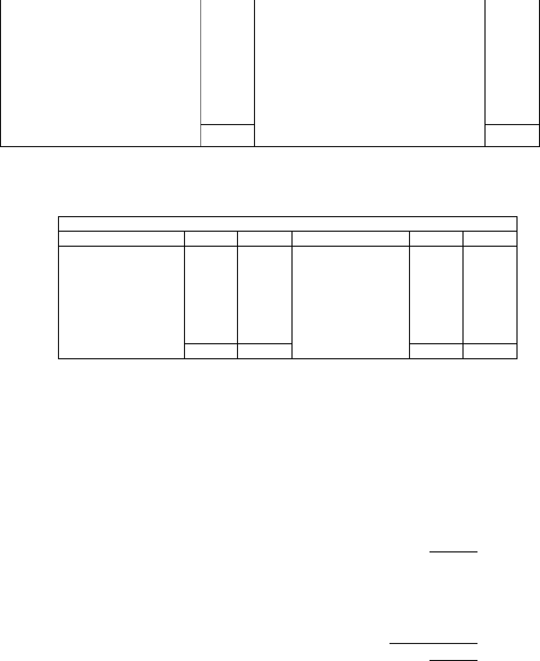
81
To Appropriation of retained earnings By Transfer from excess provisions
To Loss on sale of fixed assets By Appreciation in the value of fixed assets
To Dividend By Dividend received
To Proposed Dividend By Profit on the sale of fixed assets
To Provision for Taxation By Funds from Operations
To Closing Balance of P & L A/c
To Funds lost in Operations (B/F)
Let us take an example of the funds from operations.
Illustration 4.2: Following are Balance Sheet of a Limited Co. as on 31st Dec.2003 and
2004. Balance Sheet
Liabilities 2003 2004 Assets 2003 2004
Share Capital 61,000 74,000 Plant 45,000 43,000
Reserves 13,000 15,500 Building 50,950 48,000
Creditors 28,000 24,000 Stock 20,500 18,800
Bank Overdraft 18,000 Debtors 20,000 16,200
Provision for Taxation 8,000 8,500 Cash 150 180
Profit & Loss A/c 8,600 8,800 Cash at Bank 2,100
Goodwill 2,520
1,36,600 1,30,800 1,36,600 1,30,800
Taking into account the following information, calculate funds from operations: -
1) Interim Dividend was paid Rs.2,000.
2) Dividend proposed for Rs. 4,000.
3) Provision of Rs.9,000 was made for Income Tax.
4) Rs. 2000 was written off as depreciation on Plant and Rs.2,950 on Building.
5) Profit on Sale of Fixed Investment Rs. 1,500.
Solution:
Calculation of net profit for 2003
Rs. Rs.
Credit balance of P & L A/c on 31Dec. 2003 8,800
Less: Credit Balance of P& LA/c on 31Dec.2002 8,600
200
Add:
Interim Dividend 2,000
Proposed Dividend 4,000
Provision made for Income Tax 9,000
Provision Made for Reserve 2,500 17,500
Net Profit During the Year 17,700
Calculation of Funds From Operations

82
Net Profit During the Year 17,700
Add:
Depreciation on Building 2,950
Depreciation on Plant 2,000 4,950
22,650
Less:
Profit on sale of Fixed Investment 1,500
Profit from Business Operations 21,150
The alternative method for calculation of Funds from operations is as follows:
Adjusted Profit and Loss A/c
To Interim Dividend 2,000 By Opening Balance 8,600
To Dividend Proposed 4,000 By Profit on Sale of Investment 1,500
To Provision for Income Tax 9,000 By Profit From Business Operations 21,150
To Provision for Reserve 2,500 (Balancing Figure)
To Plant A/c(Depreciation) 2,000
To Building A/c (Depreciation) 2,950
To Closing Balance 8,800
31,250 31,250
2. External Source: These sources include:
i) Issue of Share Capital: One of the source of collection of the funds is issuance
of the new share that may be preference share issue or equity share issue. Not only
the new issue but also the call made on the partly paid share is also considered as
the source of the funds because it generates inflow of funds. The premium charged
on the time of issue is also considered, as inflow of funds and similarly the
adjustment for the discount provided on the time of issue should be made. If the
shares are issued in respect of another consideration rather than cash then it will
not be considered as a source of funds.
ii) Issue of Debenture and Raising of Loans: Just like the shares issue of debenture
and raising of loans are also a source of funds and the same adjustment regarding
the premium and discount should be made as in case of the issuance of the share.
iii) Sale of the Fixed Assets and Long-term Investments: One can increase the
funds in the concern by selling their investment they have made in different
alternatives and in fixed assets just like plant, machinery, building etc. but one
83
thing that should be remembered that if the assets are exchanged with rather than
cash that will not a source of funds.
iv) Non-Trading Receipts: Any non-trading receipts just as rent received, interest
received, dividend received and refund of tax or any another non-operating
income generates the inflow of cash will be treated as source of funds.
v) Decrease in Working Capital: If the working capital decreases in comparison of
previous year in the release of funds from the working capital so that will be
termed as source of funds.
Application or Uses of Funds
The other side of the funds flow statement is application of funds that side shows how the
funds procured from different sources are allocated or used. There may be following uses
or applications of the funds:
1) Funds lost in Operations: Sometimes the result of trading in a certain year is a loss
and some funds are lost during that trading period. Such loss of funds means outflow
of funds so that item if treated as an application of funds.
2) Redemption of the Preference Share Capital: A company can’t redeem its equity
share within its life time but can redeem their preference share as the result of
redemption of preference share an outflow of funds takes place. So the redemption of
the shares is written in the application side of the funds flow statement. One thing
should be remembered is that the premium provided on the redemption will also
considered as an application.
3) Repayment of Loans & Redemption of Debentures: As share the repayment of
loans and redemption of debenture also leads a outflow of cash so these items are also
treated as application of the funds.
84
4) Purchase of any Non-current or Fixed Asset: If the businessman purchases any
fixed asset or making investment for the long time period that will also generate a
outflow of funds and treated as an application of funds. But if the fixed asset is
purchased in exchange of any other consideration rather than cash that will not treated
as application of funds.
5) Payment of Dividend & Tax: Payment of dividend and tax are also applications if
funds. It is the actual payment of dividend and tax, which should be taken as an
outflow of funds and not the mere declaration of the dividend or creation of a
provision for taxation.
6) Any other Non-trading Payment: Any payment or expenses not related to the
trading operations of the business amounts to outflow and is taken as an application of
funds. The examples could be drawing in case of sole trader or partnership firm, loss
of cash.
4.6 PARTIES INTERESTED IN FUND FLOW STATEMENT
Funds flow statement is useful for different parties interested in the
business. They include owner or shareholder, financial institutions,
employees etc.
1. Owners or Shareholders: Owners and Shareholders are interested in ascertaining the
financial position of the concern. Funds flow statement helps them to find out:
i) Whether the business has enough funds to pay dividend at reasonable rates?
ii) Whether the business is in a position to meet its present liabilities in time?
iii) Whether the management is making effective use of funds at their disposal?
2. Financial Institutions: The financial institutions are interested in the
safety of their funds. A careful analysis of the fund flow statement will
help them in ascertaining:
85
i) Overall creditworthiness of the enterprise.
ii) The resources from which the enterprise will be in a position to
make repayments of the loans taken.
3. Employees: The employees have also a stake in the business. Their
growth and security of job depends upon the profitability of the firm
which is directly related to effective utilisation of the funds by the
enterprise. The employees can ascertain firm the funds flow statement
regarding effective use of funds by the management during a particular
period. The funds should be managed in a manner that the business is in
a position to make payment of salaries to the employees in the time
beside meeting other business costs.
It is a useful practice in business firms to prepare projected funds flow
statement for a number of years to predict the future availability of the
funds and their utilization. All this will help the firm in better planning of
its resources and their utilizations.
4.7 SOME TYPICAL ITEMS WHICH REQUIRE PARTICULAR CARE
The following items require particular care while preparing a funds flow
statement.
1. Digging out the hidden information: While preparing a funds flow
statement one has to analyze the given balance sheet. Items relating
to current account to be shown in the schedule of change in working
capital. But the non-current items have to be further analyzed to fund
out the hidden information in regard to sale or purchased of non
current assets, issue or redemption of share capital, raising or
repayment of long-term loans, transfer to reserves and provisions etc.
the hidden information can be digged out either by preparing working
notes in the statement form or preparing concerned accounts of non-
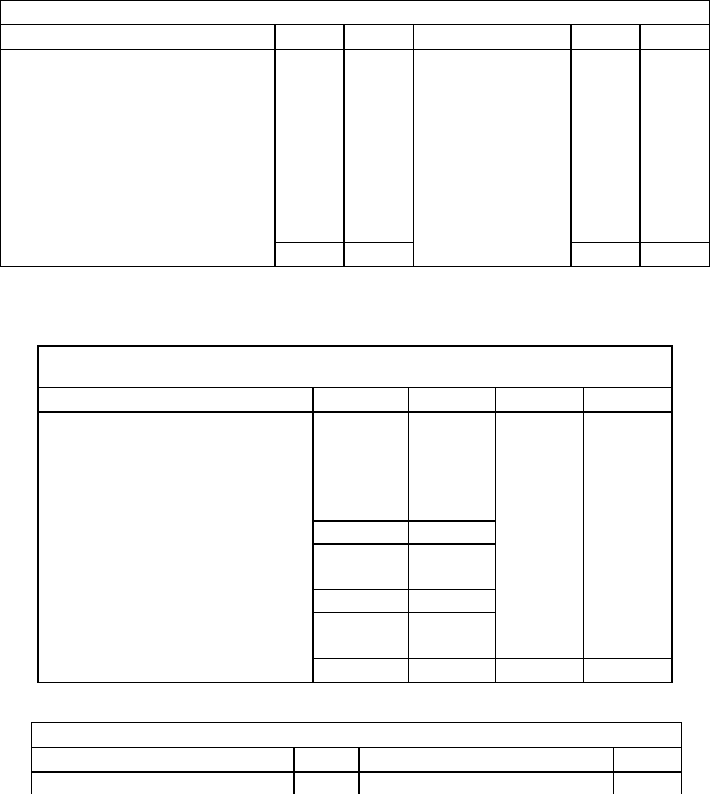
86
current assets and non-current liabilities. Both of these methods have
been clarified by following illustration:
Illustration 4.3 The following is the Balance Sheet of Anil Corporations Ltd.
as on 31st Dec. 2003 and 2004. You are required to prepare a Schedule of
Changes in Working Capital and a Funds Flow Statement.
Balance Sheet of Anil Corporation Ltd.
Liabilities 2003 2004 Assets 2003 2004
Share Capital (Paid up): Land & Buildings 60,000 50,000
11% Cumulative Preference Share 30,000 Plant and Machinery 30,000 50,000
Equity Shares 1,10,000 1,20,000Sundry Debtors 40,000 48,000
General Reserve 4,000 4,000 Stock 60,000 70,000
Profit & Loss A/c 2,000 2,400 Bank 2,400 7,000
9% Debentures 12,000 14,000 Cash 600 1,000
Provision for Taxation 6,000 8,400
Proposed Dividend 10,000 11,600
Current Liabilities 49,000 35,600
1,93,000 2,26,000 1,93,000 2,26,000
Solution:
Schedule of Changes in Working Capital
Particulars 2003 2004 Increase Decrease
Current Assets:
Sundry Debtors 40,000 48,000 8,000
Stock 60,000 70,000 10,000
Bank 2,400 7,000 4,600
Cash 600 1,000 400
1,03,000 1,26,000
Current Liabilities:
Current Liabilities 49,000 35,600 13,400
49,000 35,600
Working Capital (CA-CL) 54,000 90,400
Net increase in Working Capital 36,400 36,400
90,400 90,400 36,400 36,400
Funds Flow Statement
Sources Rs. Applications Rs.
Issue of the Preference Shares 30,000 Purchase of Plant and Machinery 20,000

87
Issue of the Equity Shares 10,000 Provision for Taxation* 6,000
Issue of the Debentures 2,000 Proposed Dividend** 10,000
Sale of the Land and Buildings 10,000 Net Increase in Working Capital 36,400
Funds from Operations 20,400
72,400 72,400
* For 2003 assumed to be paid
** For 2003 assumed to be paid
Working Notes:
1. As current Liabilities are separately given, provision for taxation and proposed
dividend has not been taken as current liabilities.
2. Calculations of Issue of Preference Shares:
Preference share in beginning of 2004 --------
Preference share raised during the year 2004 30,000
Preference share at the end of 2004 30,000
3. Calculation of Issue of Equity Share:
Equity Share Capital In the beginning of 2004 1,10,000
Equity Share Capital at the end of 2004 1,20,000
Equity Share Capital issued during the year 2004 10,000
4. Issue of Debenture:
9% Debenture in the beginning of 2004 12,000
9% Debenture at the end of the year 2004 14,000
9% Debenture issued during the year 2004 2,000
5.Provision for taxation and proposed dividend for 2003 have been presumed
to be paid in 2004.
6.Calculations of Sale of Land and Buildings:
Opening Balance of Land & Building in 2004 60,000
Closing Balance of Land & Building in 2004 50,000
Land and Building purchased during the year 2004 10,000
7.Purchase of Plant & Machinery:
Opening Balance in 2004 30,000
Closing Balance in 2004 50,000
Purchased during the year 20,000
8.Calculation of Funds from Operations:
Closing Balance of P & L A/c in 2004 2,400
Add: Non-fund and Non-operating items
Debited to P & L A/c:
Provision for taxation 8,400
Proposed Dividend 11,600
22,400
Less: Opening Balance of P & L A/c 2,000

88
Funds from Operations 20,400
2. Investments: The treatment of the investment depends on the nature of the
investment. If the investment is made in short term investment instrument then it is
considered as current assets and shown in the schedule of changing in working
capital. Or if the investment is made in long term instrument then the difference
between opening and closing balance is treated as purchase or sale of investment and
will be shown in the funds flow statement and appropriate adjustment regarding the
profit or loss on sale of investment is made during the calculation of funds from
operations.
3. Provision for Taxation: If the provision for taxation is treated as current liability
then it should be shown in the schedule of changing in working capital. If it treated, as
non-current liability then opening balance will be shown in the funds flow statement
by assuming it as paid for last year and closing balance will be added back in the
profit if it is debited earlier in P & L A/c for calculation of Funds from Operations.
4. Proposed Dividend: Proposed dividend also can be treated in two ways as same as
provision for taxation. And adjustment will be same as in the case of provision for
taxation.
5. Interim Dividend: The expression interim dividend denotes a dividend paid to the
members of the company during a financial year, before the finalization of annual
accounts. The dividend paid or declared in between the two annual general meeting
should be added back while calculating funds from operations. However, if the figure
of profit is taken prior to the debit of interim dividend this adjustment is nor required.
The interim dividend is also an application of funds and has to appear on the
applications side of funds flow statement.

89
6. Provision against Current Assets: The provision against the current assets either
deducted from their respective opening and closing balances before entering in the
schedule of changes in working capital or the difference between the opening and
closing balance if excess provision has been created may be treated as appropriation
of profit and should be added back while calculating the funds from operations. The
amount of excess provision will not be shown in the schedule of changes in working
capital.
7. Depreciation: depreciation means decrease in the value of an asset due to wear and
tear, lapse of time, obsolesce and accident. Depreciation is taken as an operating
expense while calculating operating profit. When we make the entry of depreciation
profit and loss account is debited while fixed asset account is credited with the
amount of depreciation. Since, both the accounts are non-current accounts so
depreciation is treated as a non-fund item. It is neither a source nor a application of
funds so it is added back to operating profit to find out funds from operations.
Illustration 4.4: The following schedule shows the balance sheets in
condensed form of Bharat Carbons Limited at the beginning and end
of the year:
Particulars 1/1/2002 31-12-2002
Cash 50,409 40,535
Sundry Debtors 77,180 73,150
Temporary Investment 1,10,500 84,000
Prepaid Expenses 1,210 1,155
Inventories 92,154 1,05,538
Surrender Value of Life Policies 4,607 5,353
Land 25,000 25,000
Other Fixed Assets(Including Machinery) 1,47,778 1,82,782
Debenture Discount 4,305 2,867
5,13,143 5,20,380
Sundry Creditors 1,03,087 95,656

90
Outstanding Expenses 12,707 21,663
4% Mortgage Debentures 82,000 68,500
Accumulated Depreciation 96,618 81,633
Allowance for Inventory Loss 2,000 8,500
Reserve for Contingency 1,06,731 1,34,178
Surplus in P/L A/c 10,000 10,250
Equity Share Capital 1,00,000 1,00,000
5,13,143 5,20,380
Additional Information:
1. Net profit for the year 2002 as P/L A/c is Rs. 49,097.
2. 10% cash dividend was paid during the year.
3. The premium on life policies Rs. 2,773 was paid during the year, which Rs. 1,627 has
been written off from P/L A/c.
4. New machinery was purchased for Rs. 31,365 and machinery costing Rs. 32,625 was
sold during the year. Depreciation on machinery sold had accumulated to Rs. 29,105
at the date of the sale. It was sold as scrap for Rs. 1,500.
5. The Mortgage debentures mature at the rate of Rs. 5,000 per year. In addition to the
above The Company purchased and retired Rs. 8,500 of the debentures at Rs. 103.
Both the premium on retirement and the applicable discount were charged to P/L A/c.
6. The allowance for inventory loss was credited by a charge to expenses in each year to
provide for obsolete items.
7. A debit to reserve for contingencies of Rs. 11,400 was made during the year. This
was in respect of settlement of past tax liability.
You are required to prepare a statement showing the sources and applications of funds for the
year 2002.
Solution:
Statement of Changes in Working Capital
Particulars 1/1/2002 31/12/02 Increase Decrease
Current Assets:
Cash 50,409 40,535
9,874
Sundry Debtors 77,180 73,150 4,030
Temporary Investment 1,10,500 84,000 26,500
Prepaid Expenses 1,210 1,155 55
Inventories 92,154 1,05,538 13,384
3,31,453 5,20,380
Current Liabilities:
Sundry Creditors 1,03,087 95,656 7,431
Outstanding Expenses 12,707 21,663 8,956

91
Allowance for Inventory Loss 2,000 8,500 6,500
1,17,794 1,25,819
Working Capital 2,13,659 1,78,559
Net Decrease in W.C. 35,100 35,100
2,13,659 2,13,659 59,915 59,915
Note :
1) Surrender value of the life insurance policy is not considered as a current asset.
2) Allowance for inventory loss which is a provision against the current asset has been treated
as a current liability like provision for doubtful debts not to be an appropriation of profits.
Statement of Sources and Applications of Funds for the year ended 31/12/02
Sources Rs. Applications Rs.
Funds from Operation 68,957 Redemption of debentures 13,755
Sale of Machinery as scrap 1,500 Purchase of machinery 31,365
Net Decrease in W.C. 35,100 Purchase of other fixed assets 36,264
Payment of life insurance premium 2,773
Payment of Tax 11,400
Payment if Dividend 10,000
1,05,557 1,05,557
Working Notes:
4% Mortgage Debentures A/c
To Cash 5,000 By Balance b/d 82,000
To cash 8,755 By Adjusted P/L A/c(Premium) 255
To Balance c/d 68,500
82,255 82,255
Other Fixed Assets (including machinery)
To Balance b/d 1,47,778By Accumulated Depreciation 20,105
To Cash(Purchase) 31,365 By Cash (Sale) 1,500
To Cash(Purchase)balancing figure 36,264 By Adjusted P/L A/c(loss) 2,020
BY Balance c/d 1,82,782
2,15,407 2,15,407
Accumulated Depreciation A/c
To Other Fixed Assets A/c 29,105By Balance b/d 96,618
To Balance c/d 81,633By Adjusted P/L A/c(b/f) 14,120
1,10,738 1,10,738
Reserve for Contingency A/c
To Tax Paid 29,105 By Balance b/d 1,06,731
To Balance c/d 1,34,178By Adjusted P/L A/c(b/f) 28,847
1,45,578 1,45,578

92
Debenture Discount A/c
To Balance b/d 4,305 By Adjusted P/L A/c(b/f) 1,438
By Balance c/d 2,867
4,305 4,305
Life Policy A/c
To Balance b/d 4,607 By Adjusted P/L A/c 1,627
To Cash (Premium Paid) 2,773 By Adjusted P/L A/c 400
( Rs 1,627 given to be transferred to
P/L A/c and Rs.400 B/F being excess
of book value over surrender value)
By Balance c/d 5,353
7,380 7,380
Adjusted Profit & Loss A/c
To 4% Mortgage debenture a/c By Balance b/d 10,000
Premium on redemption 255 By Funds From Operation 68,957
To Accumulated Dep. A/c 14,120
To Other Fixed Assets A/c- loss on sale 2,020
To Reserve for Contingency A/c 38,847
To Debenture Discount A/c 1,438
To Dividend 10,000
To Life Insurance Policy 2,027
To Balance c/d 10,250
78,957 78,957
Note: If allowance for Inventory Loss is not treated as a currently liability net decrease in
working capital shall be Rs. 28,600.
Illustration 4.5: From the following Comparative Balance Sheet and
Income Statement of ABC Ltd. prepare a Statement of Changes in
Financial Position:
ABC Limited
COMPARATIVE BALANCE SHEET
For the year ended 31st Dec. 2003 and 2004
Particular 2003 2004
Current Assets:
Cash 70,000 50,000
Debtors 40,000 45,000
Stock 1,25,000 90,000

93
Total Current assets 2,35,000 1,85,000
Fixed Asset:
Land and Building 1,50,000 1,00,000
Plant and Machinery 22,000 2,00,000
Less: Accumulated Depreciation 82,000 80,000
Total Fixed Assets 2,88,000 2,20,000
Total Assets 5,23,000 4,05,000
Current Liabilities:
Creditors 25,000 30,000
Salaries Payable 15,000 10,000
Provision for tax 50,000 60,000
Provision for Dividend 40,000 40,000
Total Current Liabilities 1,30,000 1,40,000
Long Term Liabilities:
Bank Loan 23,000 15,000
Debentures 1,20,000 1,50,000
Total Long term Liabilities 1,43,000 1,65,000
Total Liabilities 2,73,000 3,05,000
Owner's Equity:
Share Capital 175,000 75,000
Share Premium 12,500 7,500
Reserve and surplus 62,500 17,500
Total Equities 2,50,000 1,00,000
5,23,000 4,05,000
ABC Limited
Income Statement
For the year ended 31st Dec. 2004
Particulars Rs. Rs.
Sales 5,00,000
Less: Cost of Goods Sold 2,10,000
Gross Profit 2,90,000
Less: Operating Expenses:
Office and Administration Exp. 45,000
Selling and Distribution Exp. 25,000
Interest 12,000
Depreciation 22,000 1,04,000
Operating Profit 1,86,000
Add: Gain on sale of Plant 6,000
Total Profit 1,92,000
Less: Income Tax 85,000
Net Profit 1,07,000

94
Additional Information:
1) During the year plant Rs. 50,000 (accumulated depreciation Rs. 20,000) was sold
2) The debentures of Rs. 30,000 were converted into share capital at per.
3) The company declared a cash dividend of Rs.40, 000 and a stock dividend of Rs.
20,000 for the year.
4) The company issued 5,000 additional shares, par value Rs.10 per share, at premium of
10% during the year.
Solution:
Schedule of Changes in Working Capital
Particulars 2003 2004 Increase Decrease
Current Assets:
Cash 50,000 70,000 20,000
Debtors 45,000 40,000 5,000
Stock 90,000 1,25,000 35,000
Total Current assets 1,85,000 2,35,000
Current Liabilities:
Creditors 30000 25000 5,000
Salaries Payable 10000 15000 5,000
Provision for tax 60000 50000 10,000
Provision for Dividend 40000 40000
Total Current Liabilities 1,40,000 1,30,000
Working Capital 45,000 1,05,000 70,000 10,000
Increase in Working Capital 60,000 60,000
Total 1,05,000 1,05,000 70,000 70,000
Funds Flow Statement
Sources:
Funds from Operations 1,21,000
Sales of plant 36,000
Loan from bank 8,000
Issue of share 55,000
2,20,000
Applications:
Purchase of land & Building 50,000
Purchase of Plant & Machinery 70,000
Payment of Dividend 40,000
Increase in Working capital 60,000
2,20,000
Note: Stock dividend and debenture converted into share do not find place in a funds flow
statement because these items are not affecting the position of the funds in the concern.

95
Working Notes: Adjusted Reserve and Surplus A/c
To proposed Dividend 60,000 By Balance b/d 17,500
To accumulated Depreciation 22,000 By Plant and Machinery 6,000
To Balance b/d 62,500 (Profit on Sale)
By Funds from Operations 1,21,000
1,44,500 1,44,500
Plant and Machinery A/c
To Balance b/d 2,00,000By Accumulated Depreciation 20,000
To Adjusted Reserve and Surplus A/c 6,000 By Cash (Sale) 36,000
To Cash (Purchase - B/F) 70,000 By Balance c/d 2,20,000
2,76,000 2,76,000
Accumulated Depreciation A/c
To Plant A/c 20,000 By Balance b/d 80,000
To Balance c/d 82,000 To Adjusted Reserve and Surplus A/c 22,000
(Depreciation)
1,02,000 1,02,000
Further practice can be done with the help of textbooks.
4.8 SELF-ASSESSMENT QUESTIONS
1. What is the Funds Flow Statement? Examine its managerial uses.
2. “Funds flow statement represents a stock to flow linkage”, Justify.
3. Discuss the Procedure of making a Funds Flow Statement.
4. What are the Causes for Change in Working Capital? Discuss.
5. Briefly discuss the meaning, importance and objectives of the Funds Flow
Statement.
6. From the following Balance Sheet of a company you are required to prepare 1) a
statement showing changes in working capital 2) a statement of sources and
applications of the funds.

96
Balance Sheet
Particular Jan.2003 Jan.2004
Cash 40,000 44,400
Account Receivable 10,000 20,700
Inventories 15,000 15,000
Land 4,000 4,000
Building 20,000 16,000
Equipment 15,000 17,000
Accumulated Depreciation -5000 -2,800
Patents 1,000 900
1,00,000 1,15,200
Current Liabilities 30000 32,000
Bonds Payable 22,000 22,000
Bonds Payable Discount -2,000 -1,800
Capital Stock 35,000 43,500
Retained Earnings 15,000 19,500
1,00,000 1,15,200
Additional Information:
1. Income for the period Rs.10,000
2. A building that cost Rs.4000 and which had a book value of Rs.1000 was sold
for Rs. 1400.
3. The depreciation charge for the period was Rs. 800.
4. There was Rs. 5000 issue of common stock.
5. Cash Dividend Rs. 2000 and a Rs. 3500 stock dividend were declared.
[Ans. Net Increase in working capital: Rs. 13,100 , Source of Funds: Rs. 17,100,
Application of funds: Rs. 4,000 Funds From Operations: Rs. 10,700]
7. A balance Sheet of retained earning of X Ltd. is given below:
Balance of retained earning, 1st Jan. 2003 3,25,600
Add: Net Profit after tax. 6,48,480
Tax Refund 25,470
9,99,550
Less: Loss on sale of Plant & Machinery 14,460
Goodwill written off 95,370
Dividend Paid 4,70,350
5,80,180
Balance of Retained Earning, 31st Dec.2003 4,19,370
Additional Information:

97
1. Plant and Machinery having a written off value of Rs.54,360 was sold on
Oct. 200.
2. Depreciation of Rs.68,250 has been deducted while arriving at net profit for
the year.
3. Plant and Machinery was purchased during the year at a cost of Rs. 1,60,000
but the payment was made in the form of 8% debentures of Rs. 100 Each for
the same.
4. Rs. 72,800 dentures have been redeemed during year 2003.
You are required to prepare a statement of Sources and Applications of the funds for
the Year ended on 31st Dec.2003.
[Ans. Funds from operations Rs. 7,16,730 Funds flow statement. Rs.7,82,100
increase in the working capital Rs.2,38,950]
8. The following is the Balance Sheet of Sri Krishna Limited:
As on As on As on As on
31/3/2002 Liabilities 31/3/2003 31/3/2002 Assets 31/3/2003
(in Lakhs) (in Lakhs) (in Lakhs) (in Lakhs)
Share capital: 15 Plant 18.00
100.00 Equity Shares of Rs. 100
Each 15.00 6.00 Stock 3.00
9% redeemable preference 15.00 Debtors 10.00
Share of Rs. 100 each Rs.50 1.00 Cash Balance 1.00
5.00 Called up Nil 1.00 Misc. Expenditure 4.00
0.25 Share Premium Nil
Nil Capital Redemption Reserve 5.00
10.00 General Reserve 7.00
2.75 Profit & Loss A/c 3.00
10.00 Other Liabilities 6.00
38.00 36.00 38.00 36.00
Further information furnished:
1. The company declared a dividend of 20% to equity share on 30/6/2002.
2. The company issued notice to preference share for redemption at a premium
of 5% on 1/7/2002 and the entire proceeding were completed before
15/8/2002/in accordance with the law after making a call of Rs. 50 per share,
so as to make shares fully paid.
3. The company provided depreciation at 10% on the closing of Plant. During
the year one plant of book value Rs. 1,00,000 was sold at loss of Rs. 25,000.
98
4. There was no change in the schedule of debtors as on 31/3/2002. However,
as the company felt that certain debtors were doubtful of recovery, a
provision was made in the account.
5. Miscellaneous expenditure included Es.5 lakh shares issue and other
expenses paid during the year.
Prepare funds flow statement for the year ended 31/3/2003.
[ Ans. Net decrease in working capital. Rs. 4 lakh, funds flow statement
Rs.24,06,250 funds from operations. Rs. 9,31,250]
4.9 SUGGESTED READINGS
1. Pandey, I.M., Management Accounting, Vikas Publishing House, N.Delhi
2. Horngren & Sundem, Introduction to Management Accounting, Prentice Hall of
India, N.Delhi.
3. Anthony R.N. and Reece J.S., Management Accounting Principles, 6th ed.,
Homewood, Illinois, Richard D.Irwin, 1995.
4. Hansen & Mowen, Management Accounting, Thomson Learning, Bombay.
5. Anthony Robert and Hawkins David, Accounting: Text & Cases, McGraw Hill,
1999
6. Mittal, S.N., Management Accounting and Financial Management, Shree Mahavir
Book Depot, N.Delhi.
7. Jain, S.P and Narang, K.L., Advanced Cost Accounting, Kalyani Publishers,
Ludhiana.
8. Gupta, R.L., and Radha Swamy, M, Advanced Accounting, Sultan chand & Sons,
N.Delhi.
9. Khan, M.Y. and Jain, P.K., Management Accounting, TMH, N.Delhi.

99
Objectives: After reading this chapter you will be able to: prepare a statement of changes
in cash; make out a statement of sources and applications of cash; and
understand that why after a high profit cash position become worst.
Lesson Structure:
5.1 Introduction
5.2 Meaning
5.3 Purpose and Uses
5.4 Structure of Cash Flow Statement
5.5 Treatment of Some Typical Items
5.6 Format of Cash Flow Statement
5.7 Procedure for preparing Cash Flow Statement
5.8 Limitations of Cash Flow Statement
5.9 Comparison between Cash Flow Statement and Funds Flow Statement
5.10 Self-Assessment Questions
5.11 Suggested Reading
Subject: Management Accounting
Subject Code: 105 Author: Ashish Garg
Lesson No: 5 Vetter: Dr. B.S.Bodla
CASH FLOW STATEMENT
100
5.1 INTRODUCTION
The statement of changes in financial position based on working
capital is of immense use in long-range financial planning. The long-
term financing and investment activities are specifically portrayed.
The net working capital requirements are shown as residual figures.
However, the working capital concept may conceal or exclude too
much. It treats increases in inventories and account receivable as
equaling to an increase in bank overdraft. This is not a correct
treatment. In fact, accrued expenses like wages and salaries may
become payable in next 10 days or so: sundry creditor’s bills may fall
due for payment during the next one month, where as bank overdraft
may be for a longer period of, say three months or even more.
Similarly, inventories and account receivables undergo a
transformation before they become money assets. It is possible that
there is sufficient net working capital as revealed by the statement of
changes in financial position, and yet the firm may be unable to meet
its current liabilities as and when they fall due. It may be due to a
sizeable piling up of inventories and an increase in debtors. Caused by
a slow-down in collections. The firm’s failure to meet its short-term
commitments, in spite of its sound long-range financial position and
adequate profitability, may plunge it to technical insolvency.
Therefore, in making plans for the more immediate future, the
management is vitally concerned with a statement of cash flow, which
provides more detailed information. Such a statement is useful for
the management to assess its ability to meet obligation to trade
creditors, to pay bank loans, to pay interest to debenture-holders and
dividends to its shareholders. Furthermore, the projected cash flow
statement prepared month wise or so can be useful in presenting
information of excess cash in some months and shortage of cash in
others. By making available such information in advance the
statement of cash flow enables the management revise its plan. So
101
avoid the technical insolvency and to get aware about the short-term
liquidity position management have to make Cash Flow Statement.
5.2 MEANING OF THE CASH FLOW STATEMENT
Cash Flow Statement is a statement that describes the inflow
(sources) and outflow (applications) of cash and cash equivalent in an
enterprise during a specified period of time. Such a statement
enumerates net effect of the various business transactions on cash
and its equivalent and takes into account receipts and disbursement
of cash. Cash flow statement summaries the causes of changes in
cash position of a business enterprise between dates of two balance
sheets. According to AS-3 (revised), an enterprise should prepare a
cash flow statement and should present it for each period for which
financial statements are prepared. The term cash, cash equivalent and
cash flow are used in the statement with the following meanings:
Cash comprises cash on hand and demand deposit with bank.
Cash Equivalents are short term highly liquid investments that are
readily convertible into known amounts of cash and which are subject
to an insignificant risk of changes in value. Cash equivalent are held
for the purpose of meeting short term cash commitments rather than
for investment or other purposes. An investment normally qualifies as
a cash equivalent only when it has a short-maturity, of say, three
months or less from the date of acquisitions.
Cash flow means movement of funds that may be toward outside
called outflow of cash and that may be from outside to inside business
called inflow of cash. In another words flow of cash is said to have
taken place when any transaction makes changes in the amount of
cash and cash equivalent before happening of the transaction.
Cash flows exclude movements between items that constitute cash or
cash equivalent because these components are part of the cash
102
management of an enterprise rather than part of its operating,
investing and financing activities. Cash management includes the
investment of excess cash in cash equivalent.
In another words a cash flow statement is a statement depicting
changes in cash position from one period to another. For example, if
the cash balance of a business is shown by its Balance Sheet in 31st
Dec. 2003 at Rs. 20,000 while the cash balance as per its Balance
Sheet on 31St Dec. 2004 is Rs.30,000, there has been an inflow of
cash of Rs.10,000 in the year 2004 as compared to the year 2003. The
cash flow statement explains the reasons for such inflows or outflows
of cash, as the case may be. It also helps management in making
plans for the immediate future. A projected cash flow will be available
to meet obligation to trade creditors, to pay bank loans and to pay
dividend to the shareholders.
5.3 PURPOSE AND USES OF CASH FLOW STATEMENT
The main purpose of the statement of cash flows is to provide relevant
information about the cash receipts and cash payments of an
enterprise during a period. The information will help users of financial
statements to assess the amounts, timing and uncertainty of
prospective cash flows to the enterprise. The statement of the cash
flows is useful to them in assessing an enterprise’s liquidity, financial
flexibility, profitability and risk. It also provides a feedback about the
previous assessments of these factors. Investors, analyst, creditors,
managers and others will find the information in the statement of
cash flows helpful in assessing the following:
1. It is very useful in the evaluation of cash position of a firm.
2. A projected cash flow statement can be prepared in order to know
the future cash position of a concern so as to enable a firm to plan
and coordinates its financial operations properly.
103
3. A comparison of historical and projected cash flow statement can
be made so as to find the variation and deficiency or otherwise in
the performance so as to enable the firm to take immediate and
effective actions.
4. A series of intra firm and inter firm cash flow statement reveals
whether the firm’s liquidity is improving or deteriorating over a
period of time.
5. Cash flow statement helps in planning the repayment of loans,
replacement of fixed assets and other similar long term planning of
cash.
6. Cash flow analysis is more useful and appropriate than funds flow
analysis for short-term financial analysis as in a very short period
it is cash, which is more relevant, then the working capital for
forecasting the ability of the firm to meet its immediate obligations.
7. Cash flow statement prepared according to AS-3 is more suitable
for making comparison than the funds flow statement, as there is
no standards format used for the same.
8. Cash flow statement provides information of all activities classified
under operating, investing and financing activities.
5.4 STRUCTURE OF CASH FLOW STATEMENT
According to AS-3, the cash flow statement should report cash flows
during the period classified by operating, investment and financing
activities as follows:
• Cash flow from operating activities
• Cash flow from investing activities
104
• Cash flow from financing activities
1. Cash flow from operating activities involves cash generated by
producing and delivering goods and providing services. Cash inflow
includes receipts from customers for sales of goods and services
(including collection of debtors). Cash outflow from operating activities
include payments to suppliers for purchase of material and for
services, payment to employees for services and payment to
governments for taxes and duties. Then by comparing the inflow and
outflow of cash we can determine the net value of cash flows. If the
inflows are more than outflows then it is called cash generated from
operating activities or if cash outflows are more than cash inflows
then it is called cash lost in operating activities. This cash flow is a
key indicator of the extent to which the operations of the enterprise
have generated sufficient cash flows to maintain the operating
capability of the enterprise, pay dividend, repay loans and make new
investments without recourse to external sources of financing.
Information about the specific component of historical operating cash
flows is useful, in conjunction with other information, in forecasting
future operating cash inflows.
Examples of cash flows from operating activities are:
• Cash receipts from the sale of goods and rendering the
services.
• Cash receipts from royalties, fees, commission and other
revenue.
• Cash payment to suppliers of goods and services.
• Cash payment to and on behalf of employees.
• Cash receipts and cash payment of an insurance enterprise for
premium and claims, annuities and other policy benefits.
105
Cash payment and refund of income tax unless can be specifically
identified with financing and investing activities.
• Cash receipts and payments relating to futures contract, forward
contracts, option contracts and swap contracts when the contracts
are held for dealing or trading purpose.
Some transactions, such as the sale of an item of plant, may rise to a
gain or loss that is included in the determination of the net profit or
loss. However, the cash flow relating to such transactions are cash
flows from investing activities.
2. Cash flow from investing activities involves the cash generated by
making and collecting loans and acquiring and disposing of debts and
equity instruments and fixed assets. Cash inflows from investing
activities are receipts from collection of loans, receipts from sales of
shares, debts or similar instruments of other enterprises, receipts
from sale of fixed assets and interest and dividend received firm loans
and investments. Cash outflows from investing activities are
disbursement of loans, payments to acquire share debts or similar
instruments of other enterprise and payment to acquire fixed assets.
Cash receipts and payments relating to futures contract, forward
contracts, option contracts and swap contracts except when the
contracts are held for dealing or trading purpose or the payments or
receipts are classified as financing activities.
3. Cash flows from financing activities involves cash generated by
obtaining resources from owners and providing them with a return on
their investment, borrowing money and repaying amounts borrowed
and obtaining and paying for other resources obtained from creditors
on long-term credit. Cash flows from financing activities involve the
proceeding from issuing share or other similar instrument,
debentures, mortgages, bonds and other short term or long-term
borrowings. Cash outflow from financing activities are payments of
106
dividend, payments to acquire or redeem shares to other similar
instruments of the enterprise, payment of amount borrowed, principal
payment to creditors who have extended long-term credit and interest
paid.
It is important to note down that the classification of the cash flows
into operating, investing and financing categories will depend upon
the nature of the business. For example, for financial institutions like
banks lending and borrowing are parts of their business operations.
So the income and expenditure regarding the borrowing and lending
will be included in the cash flow from operating activities.
Figure 5.1 : Structure of Cash Flows
Cash Inflows Activities Cash
Outflows
Receipts from
customers for sale
of goods and
services.
Operating Activities
Payments to suppliers
and employees for
material and services
Payments to
government for taxes
and duties.
Receipts from
sales of assets.
Payment for

107
5.5 TREATMENT OF SOME TYPICAL ITEMS
AS-3 (Revised) has also provided for the treatment of cash flow from
some peculiar items as discussed below:
1) Extraordinary items: The cash flow from extraordinary items just
like winning the lottery, loss by fire etc. either classified as arising
from operating, investing or financing activities as appropriate and
separately disclosed in the cash flow statement to enable users to
understand their nature effect on the present and future cash flows of
the enterprise.
2) Interest and Dividend: A great care have to be taken regarding the
interest and dividend as receivable of the interest and dividend is a
Receipts from sale
of investments
and from
collection of loans
Receipts from
interest and
dividend on loan
and investments
Investing Activities
Receipts from
issuance of
shares
Receipts from
issuance of
debentures
Receipts from
other long-term
borrowing
Financing Activities
Payment for purchase
of investments and for
making of loans
Payment for
dividend on share
capital
Payments for
principal on
debentures and
other borrowin
g
s
Payments for
interest on
debenture and
other borrowin
g
s
108
result of investment so it is considered as cash inflow from investing
activities while payment of dividend and interest arise due to
collection of finance so it is termed as cash outflow from financing
activities. But in case of a financial institution payment and receipts
of interest and dividend are related to their main business so these
items are treated under the head of cash flow from operating
activities.
3) Taxes on Income: Taxes paid by the business should be treated as
cash outflow generated by operating activities if nothing is stated in
the problem but if it is specified in question that the tax arise due to
financing and investing activities then that tax should be treated
under respective activities.
4) Acquisitions and Disposal of Subsidiaries and other Business
Units: The aggregate cash flows arising from acquisitions and from
disposal subsidiaries or other business units should be presented
separately and classified as investing activities. The separate
presentation of the cash flow effects of acquisitions and disposal of
subsidiaries and other business units as single line items helps to
distinguish these cash flows from other cash flows. The cash flow
effects of disposal are not deducted from those of acquisitions.
5) Foreign Currency Cash Flow: Cash flows arising from transactions in
a foreign currency should be recorded in an enterprise’s reporting
currency by applying to the foreign currency amount the exchange
rate between the reporting currency and the foreign currency at the
date of the cash flow. The effect of the changes in exchange rates on
cash and cash equivalents held in a foreign currency should be
reported as a separate part of the reconciliation of the changes in cash
and cash equivalents during the period.
Unrealized gains and loss arising from changes in foreign exchange
rates are not cash flows. However, the effect of exchange rate changes
on cash and cash equivalent held is reported in the cash flow

109
statement in order to reconcile the value of cash and cash equivalent
at the beginning and the end of the period. This amount is presented
separately from cash flows from operating, investing and financing
activities and includes the difference, if any.
6) Non-Cash Transactions: There are some transactions, which do not
affect the cash positions of the business directly but affect the capital
and asset structure of an enterprise. Such as the conversion of debts
into equity, the acquisitions of an enterprise by means of issue of
shares etc. These transactions should not be included in the cash flow
statement but due to their importance these can be shown as
additional information under the statement.
5.6 FORMAT OF CASH FLOW STATEMENT
AS-3 (Revised) has not provided any specific format for preparing a
cash flow statement. The cash flow statement should report cash flows
during the period classified by operating, investing and financing
activities. A widely used format of cash flow statement is given below.
COMPANY’S NAME:…………………………
Cash Flow Statement
For the year ended…………..
Cash flow from Operating Activities
(List of the individual inflows and outflows) ………...
Net Cash Flow from Operating Activities ………
Cash Flows from Investing Activities
(List of individual inflows and outflows) ……….
Net Cash Flows from Investing Activities ……….
Cash Flows from Financing Activities
(List of individual inflows and outflows) ……….
Net Cash Flows from Financing Activities ……….
Net increase (Decrease) in Cash and Cash Equivalents ……….
Cash and cash Equivalent at the Beginning of the period ……….
Cash and cash Equivalent at the End of the period ……….
Particulars Rs. Rs.

110
5.7 PROCEDURE FOR PREPARING A CASH FLOW STATEMENT
Let us study how to construct the cash flow statement. As shown in the format of the
cash flow statement all the cash inflows and outflows will be classified according to
operating, investing and financing activities. Following are the procedures of the
calculation of cash flow from different activities: -
Determination of cash flow from operating activities: The profit and loss accounts
shows whether an enterprise’s operations have results in profit or loss, but it does not
indicate cash inflows and cash outflows from operating activities. This is because bet
profit is computed using the accrual basis of accounting. Revenue is recorded when
earned although the cash for some of them may not have been collected, and expenses
are recorded when incurred although all of them may not have been paid in cash.
Further, depreciation, amortization and provision for doubtful debts do not reflect
cash outflows in both current and future periods. Thus, the net profit will not indicate
the net cash flow from operations. In order to arrive at net cash flow from operating
activities, it is necessary to restate revenues and expenses on a cash basis. This is done
by adjusting for the effects of transactions considered in preparing the profit and loss
account that did not involve cash inflows or cash outflows. There are two methods for
reporting the net cash flow from operating activities.
1) Direct method
2) Indirect method
1) Direct method: Under this method, cash receipts from operating
activities and cash payments for operating expenses are calculated to
arrive at cash flows from operating activities. The difference between

111
the cash receipts and cash payments is the net cash flow provided by
operating activities. Cash flow from operating activities can be
calculated as follows:
Cash Flow from Operating Activities:
Cash received from customers XXX
Cash paid to suppliers and employees (XXX)
Cash generated from operations XXX
Income tax paid (XXX)
Cash flow before extraordinary item XXX
Extraordinary item (XXX)
Net cash flow from operating activities XXX
Cash received from customers: Cash receipts from customers from
cash sales and collections of debtors arising from credit sales. Cash
sales result in cash inflows in the current period. However, collections
from customers require additional calculations, sales from an earlier
period may be collected in the current period, sales from the current
period may be collected in future period or some debtors may not be
collected at all. As result, collections from customers in current period
are seldom equal to credit sales. The relationship among the credit
sales, change in debtors and collections from customers may be stated
in equation form as follows:
Cash received form customers= Sales + Opening balance of trade debtors (Debtors &
B/R) – Closing balance of trade debtors.
Cash paid to suppliers and employees: After calculation of cash received from
customers the second thing that would be calculated is cash paid to suppliers and
employees in lieu of services and goods received from them. Cash paid to customers
and employees can be calculated by using following equation:

112
Cash Paid to suppliers and employees = Purchases for the year as per statement of
profit + Opening trade creditors (Creditors & B/P) – Closing trade creditors + selling
and administrative expenses + prepaid expenses at the end of the year – prepaid
expenses in the beginning of the year.
Income tax paid: The amount of the income tax paid usually differs from the
estimated income tax expense, appearing on the profit and loss account. Also a part of
the income tax expenses for a year is paid in the following year. The difference
between income tax payment and income tax expense result in a change in income tax
payable. The following equation shows this relationship:
Tax paid during the year = Opening balance of tax unpaid + Provision made during
the year – Closing balance of tax unpaid.
Let us take an example to understand these treatments.
Illustration 5.1: The Board of Director of Amit ltd. was not able to decide that why
the Co. are not having adequate cash balance. The amount of profit of the company
for the year 2003 was Rs. 90,000. This was highest amount as compared to previous
years. You have been asked to prepare a Cash Flow Statement with the help of
following information using direct method.
Balance Sheet
(Rs. in thousands)
Liabilities Dec.2002 Dec.2003 Assets Dec.2002 Dec.2003
Issue and paid up capital 1,575.00 1,575.00 Long term assts 1,125.00 2.047.50
Profit and Loss A/c 157.00 225.00 Closing stock 337.50 900.00
Mortgage Loan 900.00 Prepayments 45.00 90.00
Tax unpaid 22.50 67.50 Trade debtors 112.50 450.00
Trade creditors 315.00 877.50 Cash 450.00 157.50
2,070.00 3,645.00 2,070.00 3,645.00
Statement of Profit
(For the year ended Dec.2003)

113
Particulars Rs. ,000 Rs. ,000
Sales 2,250.00
Opening stock 337.50
Add. Purchases 2205.00
2,542,50
Less Closing stock 900.00 1642.50
Gross profit 607.50
Less:
Administrative expenses 247.50
Depreciation 180.00
Taxes (Provision) 90.00 517.50
Net Profit 90.00
Payment of dividends 22.50
67.50
Add. Profit and loss a/c (Jan.2003) 157.50
Balance on Dec. 2003 225.00
You are also informed that a new building was purchased on 15th June 2003 for Rs.
11,02,500.
Solution:
Cash Flow Statement
(For the year ended 31st Dec.2003)
Particulars Rs., 000 Rs., 000
Cash Flow from Operating Activities
Cash Received from Customers (Note-1) 1,912.50
Cash Paid to Suppliers and Employees (Note-2) (1,935.00)
Cash generated from Operating Activities (22.50)
Income Tax Paid (Note-3) (45.00)
Net Cash Used in Operating Activities (67.50)
Cash Flow from Investing Activities
Purchase of New Building (1,102.50)
Net Cash Used in Investing Activities (1,102.50)
Cash Flow from Financing Activities
Raising of Mortgage Loan 900.00
Dividend Paid (22.50)
Net Cash Provided by Financing Activities 877.50
Net decrease in cash and cash equivalent (292.50)
Opening balance of cash 450.00
Closing balance of cash 157.50
Working Notes:

114
1. Calculation of cash received from customers:
Sales for the year as per the statement 2,250.00
Add: Trade debtors in the beginning 112.50
2362.50
Less: Trade debtors at the end 450.00
Cash received from customers 1912.50
2. Calculation of cash paid to suppliers and employees:
Purchase for the year as per the statement of profit 2,205.00
Add: Trade creditors in the begging 315.00
2520.00
Less: Trade creditors at the end 877.50
Cash paid to creditors for purchase of goods (A) 1642.50
Administrative expenses as per the statement of profit 247.50
Add: Prepaid exp. at the end 90.00
337.50
Less: Prepaid Exp. In the begging 45.00
Cash paid for services (B) 292.50
Cash paid to suppliers and employees (A+B) 1,935.00
3.Calculation of tax paid:
Opening balance of tax unpaid 22.50
Add: Provision made during the year 90.00
112.50
Less: Closing balance of tax unpaid 67.50
Tax paid during the year 45.00
3) Indirect Method: Under the indirect method, the net cash flow from
operating activities is determined by adjusting net profit or loss for the
effect of:
i) Non cash items such as depreciation, provision, deferred taxes and
unrealized foreign exchange gains and losses
ii) Changes during the period in inventories and operating receivables and
payables.
iii) All other items for which cash effects are investing or financing flows.

115
The indirect method is also called the reconciliation method as it involves reconciliation of
net profit or loss as given in the profit and net cash flow from operating activities as shown in
the cash flow statement. Cash flow from operating activities by using the indirect method can
be calculated as follows:
Net Profit before Tax and Extraordinary Items XXX
Add: Non-cash and non-operating items, which have already been
Debited to P/L A/c;
Depreciation
Transfer to reserve and provisions
Goodwill written off
Preliminary expenses written off
Other intangible assets written off just as discount or loss on issue of
Shares, debentures and underwriting commission
Loss on disposal of fixed assets
Loss on sale of investment
Foreign exchange loss XXX
XXX
Less: Non-cash and non-operating items, which have already been
Credited to P/L A/c
Gain on the sale of fixed assets
Profit on sale of investment
Income from interest or dividend
Appreciation in values of fixed assets
Reserve written back
Foreign exchange gains (XXX)
Operating profit before adjustment of working capital changes XXX
Adjustment for changes in current operating assets and liabilities:
Add: Decrease in accounts of current assets (except cash and cash equivalents) XXX
Add: Increase in accounts of current operating liabilities (except Bank overdraft) XXX
Less: Increase in accounts of current assets (XXX)
Less: Decrease in accounts of current liabilities (XXX)

116
Cash generated from operation before tax
XXX
Less: Tax paid (XXX)
Cash flow before extra-ordinary items XXX
Add/Less: Extra-ordinary items XXX
Net cash flow from operating activities XXX
Let us take an example to clear the above points.
Illustration 5.2: The following are the comparative Balance Sheet of Ashish Ltd. as
on 31st Dec.2003 and 2004.
Balance Sheet
Liabilities 2003 2004
Assets
2003 2004
Share capital
(share of Rs.10 each) 3,50,000 3,70,000 Land 1,00,000 1,50,000
Profit & Loss A/c 50,400 52,800 Stock 2,46,000 2,13,500
9% Debentures 60,000 30,000 Goodwill 50,000 25,000
Creditors 51,600 59,200 Cash & Bank 42,000 35000
Temporary Investment 3,000 4000
Debtors 71,000 84,500
5,12,000 5,12,000 5,12,000 5,12,000
Other particulars provided to you are: A) Dividend declared and paid during
the year Rs.17,500 B) Land was revaluated during the year at Rs. 1,50,000
and profit on the revaluation transferred to P/L A/c. you are required to
prepare a cash flow statement for the year ended 31/12/04.
Solution:
Cash Flow Statement
(for the year ended 31St Dec.2004)
Particulars Rs. Rs.
Cash Flow from Operating Activities
Increase in the balance of P/L A/c 2,400
Adjustment for non-cash and non-operating items:
Profit on revaluation of land (50,000)
Goodwill written off 25,000
Dividend declared 17,500

117
Operating profit before working capital changes (5,100)
Adjustment for changes in current operating assets and liabilities:
Increase in creditors 7,600
Decrees in stock 32,500
Increase in debtors (13,500)
Cash generated from operating activities 21,500
Income tax paid --------
Cash flow from extra ordinary items ---------
Net cash flow from operating activities 21,500
Cash flow from investing activities -------- --------
Cash flow from financing activities
Proceeds from issue of share capital 20,000
Redemption of debentures (30,000)
Dividend paid (17,500)
Net cash used in financing activities (27,500)
Net decrease in cash and cash equivalent (6,000)
Cash and cash equivalent at the begging of the year 45,000
Cash and cash equivalent at the end of the year 39,000
5.8 LIMITATIONS OF CASH FLOW STATEMENT
Despite a numbers of uses, cash flow statement suffers from the
following limitations:
1. As cash flow statement is based on cash basis of accounting, it ignores the basic
accounting concepts of accrual basis.
2. Some people feel that as working capital is a wider concept of funds flow
statement provides a more complete picture than cash flow statement. So it is
based on narrow concept.
3. Cash flow statement is not suitable for judging the profitability of a firm as non-
cash charges are ignored while calculating cash flows from operating activities.
5.9 COMPARISON BETWEEN FUNDS FLOW AND CASH FLOW STATEMENT
The term funds have a variety of meaning. In narrow sense it means
cash and the statement of changes in the financial position prepared
on cash basis is called a cash flow statement. In the most popular
sense, the term funds refer to working capital and a statement of

118
changes in the financial position prepared on this basis is called a
funds flow statement. A cash flow statement is much similar to a
funds flow statement as both are prepared to summarize the causes of
changes in the financial position of a business. However the following
are the main differences between funds and a cash flow statement.
Difference between Funds Flow Statement and Cash Flow Statement
Basis of Difference Funds Flow Statement Cash Flow Statement
1. Basis of Concept It is based on a wider concept of
funds, i.e. working capital
It is based on a narrow concept of
funds, i.e. cash
2. Basis of Accounting It is based on accrual basis of
accounting.
It is based on cash basis of
accounting.
3. Schedule of changes
in working capital
Schedule of changes in working
capital is prepared to show the
changes in current assets and current
liabilities.
No schedule of changes in
working capital is prepared.
4. Method of Preparing Funds flow statement reveals the
sources and applications of funds.
The net difference between sources
and applications of funds represents
net increase in working capital.
It is prepared by classifying all
inflows and outflows in term of
t
ing , investing and financing
t
ies. The net difference represents
t increase or decrease
5. Basis of Usefulness It is useful in planning intermediate
and long term financing.
It is useful in planning intermediate
and long term financing.
6.Discription It describes the reasons for change in
working capital.
It describes the reasons for changes
in cash and cash equivalent.
Illustration 5.3: Western Telecommunication Company’s profit and loss account for the year
ended January 31,2004, and its balance sheet as on Dec.2003 and Dec.2004 are as follows:
Western Telecommunication Company: Profit and Loss Account
(For the year ended Dec. 2004)
Sales Rs 5,70,000
Interest Income 2,000

119
Gain on sale of investment 7,000
Cost of goods sold 4,45,000
Depreciation Expenses 89,000
Selling and Distribution Exp. 46,000
Interest Exp. 14,000
Loss on sale of plant and machinery 3000
Profit before income tax and extraordinary items (18000)
Income Tax -----------
Profit before extraordinary items (18,000)
Extraordinary item: Insurance proceeds from Earthquake loss claim ----------
Net Profit (18,000)
WESTERN TELECOMMUNICATION COMPANY: Balance Sheet as on 31St
December
Sources of Funds 2003 2004
Shareholder funds
Equity share capital 1,55,000 85,000
Profit and loss account 1,02,000 1,20,000
Total share holder fund 2,57,000 2,05,000
Loan funds
Secured loans 97,000 57,000
Unsecured loans 1,81,000 1,91,000
Total loan funds 2,78,000 2,48,000
Current liabilities
Bill payable 6,000 9,000
Creditors 24,000 1,78,000
Income tax payable 9,000 17,000
Total current liabilities 39,000 2,04,000
Total source of funds 5,74,000 6,57,000
Applications of funds
Fixed assets
Plant and machinery 7,20,000 5,40,000
Less accumulated depreciation 3,62,000 3,05,000
Fixed assets (net) 3,58,000 2,35,000
Investment 18,000 66,000
Current assets
Inventories 1,51,000 1,19,000
Debtors (less provision of doubtful debts 8,000 & 12,000) 29,000 1,66,000
Prepaid expenses 6,000 2,000
Cash and cash equivalent 12,000 69,000

120
Total current assets 1,98,000 3,56,000
Total application of funds 5,74,000 6,57,000
Additional information:
i. Purchased machinery costing Rs.1,50,000 with cash.
ii. Sold machinery with cost of Rs.45,000 and accumulated depreciation of
Rs.32,000 for Rs.10,000.
iii. Purchased investment for Rs. 30,000.
iv. Sold investment costing Rs. 78,000 for Rs.85,000
v. Purchased machinery for Rs 75,000 in exchange for secured debentures.
vi. Issued at par share for Rs. 50,000
vii. Converted secured debentures of Rs. 20,000 to equity share of Rs. 10 at par
viii. Repaid unsecured debentures of Rs. 10,000.
ix. Redeemed secured debentures of Rs. 15,000 at par
x. Wrote off Rs. 14,000 of debtors when a customer become insolvent and provided
Rs. 10,000 for doubtful, included in selling and distribution expenses.
Required
1. Prepare the statement of cash flows according to direct method.
2. Prepare the statement of cash flows according to indirect method.
Solution:
1. Statement of Cash Flows- Direct Method
WESTERN TELECOMMUNICATION COMPANY: Statement
of Cash Flows
(For the year ended Dec.2004)
Cash Flow from Operating Activities
Cash received from customers (I) 6,97,000
Cash paid to suppliers and employees (ii) (674,000)
Cash generated from operations 23,000
Income tax Paid (iii) (8,000)
Cash flow before extraordinary items 15,000
Extraordinary items 0
Net cash provided by Operating Activities 15,000
Cash Flows from Investing Activities
Purchase of plant and machinery (150,000)
Proceeds from sale of plant and machinery 10,000
Purchase of investments (30,000)
Proceeds from sale of investment 85,000

121
Interest received 2,000
Net Cash Used in Investing Activities (83,000)
Cash Flows from Financing Activities
Proceeds from Issuance of share capital 50,000
Repayment of unsecured loans (10,000)
Redemption of secured debentures (15,000)
Interest paid (14,000)
Net Cash Provided By Financing Activities 11,000
Net Decrease in Cash and Cash Equivalent (57,000)
Cash and Cash Equivalent at beginning of period 69,000
Cash and Cash Equivalent at end of period 12,000
Supplemental schedule of non-cash investing and financing activities
1. The company purchased for Rs. 75,000 in exchange for secured debentures.
2. The company converted secured debentures of Rs. 20,000 to equity shares of Rs. 10 at
par.
Working Notes:
i. (5,70,000 + 1,78,000 - 37,000 - 14000)
ii. (4,45,000 + 46,000 - 1,19,000 - 2,000 + 9,000 + 1,78,000 + 1,51,000 +
6,000 - 6,000 - 24,000 - 10,000)
iii. (17,000 – 9,000)
2. Statement of Cash Flows – Indirect Method
WESTERN TELECOMMUNICATION COMPANY: Statement
of Cash Flows
(For the year ended Dec.2004)
Cash Flow from Operating Activities (18,000)
Net profit before income tax and extraordinary items
Adjustment to reconcile Net Profit to net cash flow from
Operating Activities
Depreciation 89,000
Provision for doubtful debts 10,000
Loss on sale of plant and machinery 3,000
Gain on sale of investment (7,000)
Interest expenses 14,000
Interest income (2,000)
Operating profit before working capital changes 89,000
Decrease in Debtors 1,27,000
Increase in inventories (32,000)
Increase in Prepaid expenses (4,000)
Decrease in bills payable (3,000)

122
Decrease in creditors (154,000)
Cash generated from operations 23,000
Income tax paid (8,000)
Cash flow before extraordinary items 15,000
Extraordinary items: Proceed from Earthquake Insurance
Claim 0
Net Cash Provided by Operating Activities 15,000
Cash Flows from Investing Activities
Purchase of plant and machinery (150,000)
Proceeds from sale of plant and machinery 10,000
Purchase of investments (30,000)
Proceeds from sale of investment 85,000
Interest received 2,000
Net Cash Used in Investing Activities (83,000)
Cash Flows from Financing Activities
Proceeds from Issuance of share capital 50,000
Repayment of unsecured loans (10,000)
Redemption of secured debentures (15,000)
Interest paid (14,000)
Net Cash Provided By Financing Activities 11,000
Net Decrease in Cash and Cash Equivalent (57,000)
Cash and Cash Equivalent at beginning of period 69,000
Cash and Cash Equivalent at end of period 12,000
Supplemental schedule of non-cash investing and financing activities
1.The company purchased for Rs. 75,000 in exchange for secured debentures.
2. The company converted secured debentures of Rs. 20,000 to equity shares of Rs. 10 at
par.
5.10 SELF-ASSESSMENT EXERCISE
1. Define the term ‘Cash Flow’. Explain the objective of cash flow analysis.
2. How does the statement of cash flows differ from the funds flow statement?
3. What is the purpose of statement of cash flows? How is it
prepared? Explain and illustrate.
4. Why is the statement of cash flow considered necessary in addition to the profit and loss
account and balance sheet?
5. Explain the procedure of preparing a cash flow statement.
6. The comparative balance sheet for Varun Ltd. are given below:
Dec.2002 Dec.2003
Assets:
Cash and Bank Balance 82,000 22,000

123
Debtors 1,04,000 24,000
Stock 1,12,000 60,000
Prepaid Expenses 22,000 14,000
Plant and Machinery 3,80,000 3,60,000
Goodwill 36,000 40,000
7,36,000 5,20,000
Liabilities:
Creditors 30,000 14,000
Provision for Depreciation 1,00,000 60,000
Debentures 1,02,000 1,02,000
Premium on Debenture Issue 12,000 18,000
Share Capital 1,90,000 90,000
Share Premium 30,000
Reserve and Surpluses 2,72,000 2,36,000
7,36,000 5,20,000
The following additional informations is available from the accounting records for 2002.
1. Debenture premium of Rs. 6,000 was amortized during the year.
2. Dividend paid Rs. 6,000.
You are required to prepare a cash flow statement.
(Answer: Net cash used in operating activities Rs.44,000; Net cash used in investing activities
Rs. 20,000; Net cash provided by financing activities Rs. 1,24,000; net increase in cash and cash
equivalent Rs. 60,000)
7. Prepare a cash flow statement of Anoop Business Corporation from the following
informations:
Balance Sheet
As on Jan, 1st & Dec. 31st 2002
Jan.1 Dec.31
Assets
Cash and Bank 40,000 44,400
Account Receivables 10,000 20,700
Inventories 15,000 15,000
Land 4,000 4,000
Business Premises 20,000 16,000
Plant and Equipment 15,000 17,000
Accumulated Deprecation (5,000) (2,800)
Patents and Trade marks 1,000 900
Total Assets 1,00,000 1,15,200
Liabilities:
Current Liabilities 30,000 32,000
Bonds Payable 22,000 22,000
Bonds Payable Discount (2,000) (1,800)
Capital Stock 35,000 43,500
Retained Earning 15,000 19,500

124
Total Liabilities 1,00,000 1,15,200
Additional Information
• Income for the period Rs.10,000.
• A building the cost Rs.4,000 and which had a book value of Rs. 1,000 was sold for
Rs. 1,400.
• Depreciation charged for the year Rs. 800
• There was Rs. 5,000 issue of capital stock
• Cash dividend of Rs. 2,000 and stock dividend of Rs. 3,500 was declared.
(Answer: Net cash operating activities Rs2,000; Net cash used in investing activities Rs. 600;
Net cash from financing activities Rs. 3,000; net increase in cash and cash equivalent Rs. 4,000)
8. From the following particulars, prepare a cash flow statement for the year ended 31st March 2004
i) Total sale for the year were Rs. 20,50,000 out of which cash sales amounted to Rs. 14,20,000.
ii) Total purchases for the year were Rs. 15,30,000 out of which cash purchases amounted to Rs.
10,20,000.
iii) Cash collected from creditors during the year amounted to Rs. 4,80,000.
iv) Cash paid to suppliers was Rs.4, 50,000.
v) Income tax paid Rs. 80,000.
vi) Equity shares of the face value of Rs. 2,00,000 were issued at a premium of 5% during the year.
vii) Rs. 25,000 was paid as dividend for the year ended 31st March 2004.
viii) Redeemable preference share of the face value of Rs. 1,00,000 were redeemed during the year at a
premium of 10%.
ix) New machinery war purchased for Rs. 30,000on 1st Jan. 2004.
x) Depreciation for the year was Rs. 40,000 where as salary and other expenses amounted to Rs.
1,80,000 out of which Rs. 20,000 are outstanding.
xi) The balance of the cash & bank as on 1st April 2003 was Rs. 85000.
(Answer: Net cash flows from operating activities Rs 1,90,000; Net cash used in investing
activities Rs. 30,000; Net cash from financing activities Rs. 75,000; net increase in cash and cash
equivalent Rs. 2,35,000)
9. The following are the Balance Sheets of GOYAL enterprises
Jan.1 Dec.31
Assets
Cash and Bank 5,000 8,000
Account Receivables 35,000 38,000
Inventories 25,000 22,000
Land 20,000 30,000
Business Premises 50,000 5,50,000
Machinery less Dep. 80,000 87,000

125
Delivery van 25,000
Total Assets 2,15,000 2,65,000
Liabilities:
Current Liabilities 35,000 40,000
Loan from Banks 30,000 25,000
Mrs. Goyal’s Loan 20,000
Capital 1,00,000 1,60,000
Hire Purchase vendor 20,000
Total Liabilities 2,15,000 2,65,000
Additional Information
The delivery van was purchased on hire purchase basis on Dec.2003, Payment of Rs. 5,000
was made at the time of agreement and the balance of amount is to be paid in 20 monthly installments
of Rs. 1,000 each together with interest @10% per annum. During the year the proprietor withdraw Rs.
25,000 for household expenses. The provision for depreciation on machinery on 1/1/03 was Rs. 27,000
and on 31/12/03 was Rs. 35,000. You are required to prepare the cash flow statement.
(Ans. Cash operating Profit Rs. 43,000)
5.11 SUGGESTED READINGS
1. Sharma, R.K. & Gupta, Shashi K., Management Accounting, Kalyani Publication,
New Delhi.
2. Horngren & Sundem, Introduction to Management Accounting, Prentice Hall of
India, N.Delhi.
3. Anthony R.N. and Reece J.S., Management Accounting Principles, 6th ed.,
Homewood, Illinois, Richard D.Irwin, 1995.
4. Hansen & Mowen, Management Accounting, Thomson Learning, Bombay.
5. Anthony Robert and Hawkins David, Accounting: Text & Cases, McGraw Hill,
1999
6. Jain, S.P and Narang, K.L., Advanced Cost Accounting, Kalyani Publishers,
Ludhiana.

126
Objective: The present lesson explains the CVP analysis. Further, it discusses the use of
the marginal costing technique for tactical decisions in different
manufacturing concerns.
LESSON STRUCTURE
6.1 Introduction
6.2 CVP Assumptions and Uses
6.3 Break-Even Point and Margin of Safety Equation Method
6.4 Graphical Representation of CVP Relationship
6.5 Marginal Costing Techniques
6.6 Summary
6.7 Self-Test Questions
6.8 Suggested Readings
6.1 INTRODUCTION
It is important for managers to ascertain the cost behavior pattern and use it to
estimate the total cost, total revenues and thereby profits at various sales volumes.
The cost revenue relationship holds for a short period. Therefore, this relationship
cannot be used to estimate long-term performance of the firm. However, this short--
term validity helps to maximise profit with given resources. For the purpose of taking
tactical decisions managers use the marginal costing techniques because these short-
term decisions influence fixed costs. To understand the use of Marginal costing
techniques, we have to study Cost-volume-profit (CVP) analysis. The Cost-volume-
profit (CVP) analysis is the study of the effects on future profit of changes in fixed
COURSE: MANAGEMENT ACCOUNTING
COURSE CODE: MC-105 AUTHOR: SURINDER S. KUNDU
LESSON: 06 VETTER: PROF. H. L. VERMA
MARGINAL COSTING AND PROFIT PLANNING

127
cost, variable cost, sales price, quantity and mix. The aim of CVP analysis is to
estimate the total cost, total revenue and thereby profit of various sales volumes.
Managers use this technique extensively to determine the break-even point and
margin of safety. Break-even point is the level of activity at which there is neither
profit nor loss. Margin of safety ratio indicates the percentage by which forecast
turnover exceeds or falls short of breakeven turnover. The CVP analysis assumes that
output is the only cost and revenue driver.
6.2 CVP ASSUMPTIONS AND USES
The assumptions of the CVP analysis are: (a) Fixed and variable cost patterns can be
established with reasonable accuracy, (b) Total fixed costs and variable cost per unit
will not change during the period under consideration, (c) Selling price will remain
constant at all sales volumes, (d) Factor price per unit (e.g. material prices, wage
rates) will remain constant at all sales volumes, (e) Efficiency and productivity will
remain unchanged during the period under consideration, (f) In a multi-product
situation, sales-mix will remain unchanged during the period, (g) Output is the only
relevant factor affecting costs and revenue, and (h) The volume of production will be
equal to the volume of sales that is accretion decoration to inventory level will be
insignificant during the period.
The uses of CVP analysis are: (a) To determine the 'Break-even point' in terms of
sales volume or sales value, (b) To ascertain the Margin of safety ratio, (c) To
estimate profits or losses at various activity levels, (d) To assess the likely effect of
management decisions such as an increase or a reduction in selling price, adoption of
a new method of production which will reduce fixed costs and increase variable costs
on the profitability of the firm, and (e) To determine the optimum selling price.
6.3 BREAK-EVEN POINT AND MARGIN OF SAFETY EQUATION METHOD
Break-even point is the sales volume or sales value at which the firm neither makes
128
profit nor incurs loss. In other words, at the break-even point, revenue equals total
costs.
6.3.1 Marginal Cost Equation
Revenue - Variable costs - Fixed costs = Operating income
Or S – V – F = P
Or S-V=F+P=C
Where S = revenue, V = total variable cost, C = total contribution F = total fixed cost
6.3.2 Contribution/Sales Ratio (C/S Ratio)
C/S = Total contribution/Total turnover x 100
Or (S-V)/S x 100 or (F+P)/S x 100
The C/S ratio represents the percentage of sales, which contributes towards fixed
costs and operating profit. CVP analysis assumes that C/S ratio does not change with
changes in output or sales volumes. It is also termed as Profit Volume ratio or PV
ratio.
6.3.3 Break-even Sales
In determining break-even sales, we need to know
(a) Fixed costs and (b) Contribution per unit or the C/S ratio.
At break-even point (BEP), total contribution equals fixed costs. Therefore, BEP in
terms of unit is calculated by dividing total fixed costs by contribution per unit. BEP
in terms of sales value is calculated by dividing total fixed costs by the C/S ratio.
Example 6.1: The following information is available from the annual budget of a
company manufacturing only one item.
Budgeted output and sales 5000 units
Budgeted selling price per unit Rs. 40
Budgeted cost per unit:
Material Rs. 15
Direct labour Rs. 5

129
Variable overhead Rs. 10
Fixed cost per unit Rs. 5 (35)
Budgeted profit per unit Rs. 5
Calculate the break-even point both in terms of the number of units and sales value.
Solution:
Contribution per unit of the given product is as follows:
Selling price Rs. 40; Variable cost: Material Rs.15; Direct labour Rs.5; Variable
overhead Rs.10 and Contribution margin per unit Rs.10. Fixed cost per unit, included
in the total cost per unit, is the average fixed cost per unit, calculated on the basis of
budgeted fixed cost (total) and budgeted output. Therefore, budgeted fixed cost (total)
= Rs. 5 x 5,000 = Rs. 25,000.
The two factors (e.g. fixed costs and contribution margin per unit) are now known to
us, and, therefore, we can calculate the BEP
BEP = Fixed Cost/Contribution per unit
= 25000/10= 2500 units.
At BEP, total contribution (2,500 x Rs. 10), that is, Rs. 25,000 is equal to fixed
costs.
C/S ratio = C per unit/ Selling price per unit
= 10/40 x 100 =25%.
BEP = Fixed cost/ C/S ratio
= 25000/25% = Rs. 1,00,000.
6.3.4 Margin of Safety
Margin of safety is the difference between the estimated sales and sales at BEP. It
provides very useful information to management, i.e. by how much can sales drop
below the budgeted sales before a loss is incurred. Margin of safety is usually
expressed as a percentage of budgeted sales.
In the example 6.1, margin of safety is (5,000 - 2,500) units or 2,500 units that is 50%
of the budgeted sales.
6.3.5 C/S Ratio and Break-even Point in a Multi-Product Situation
In a multi-product situation, it is not possible to express the break-even point in terms
of units. It is quite likely that different measuring units are used to measure sales

130
quantity of different products. Even if a single unit is used, products may not be
comparable and contribution per unit would be different. Therefore, under a multi-
product situation, BEP is calculated in terms of sale value by using weighted average
C/S ratio. Weight of each product in the sales-mix is used to calculate the weighted
average C/S ratio. The underlying assumption is that the same percentage movement
in sales of all the products in the product-mix accompanies a percentage movement in
total sales.
Break-even point is calculated with the following assumptions: (a) Constant C/S ratio
for each product; (b) Constant sales-mix; and (c) Constant fixed cost. The steps
involved in calculating the break-even points are: (a) Calculate the C/S ratio for each
product; (b) Calculate weighted average C/S ratio in relation to estimated proportion
of sales; and (c) Use the weighted average C/S ratio to calculate break-even point in
terms of sale-value.
Example 6.2: (A) SSK manufactures and sells four types of products under the
brand names A, B, C and D. The sales-mix in value comprises 3
1
33 %, 3
2
41 %,
3
2
16 % and 3
1
8 % of A, B, C and D respectively. The total budgeted sales (100%) are
Rs. 60,000 per month. Operating costs are:
Variable costs: Product: A 60% of selling price; B 68% of selling price; C 80% of
selling price; D 40% of selling price; and Fixed cost Rs. 14,700 per month. Calculate
the break-even point for the products on an overall basis.
(B) It has been proposed to introduce a change in the sales mix as follows, the total
sales per month remaining Rs. 60,000:
Product A 25%
B 40%
C 30%
D 5%
Assuming that the proposal is implemented, calculate the break-even point
Solution:

131
C/S ratio for each product
Product Variable cost to sales ratio C/S ratio (100- variable cost to sales ratio)
A 60% 40%
B 68% 32%
C 80% 20%
D 40% 60%
Weighted average C/S ratio:
Product C/S ratio (Percentage)
A 3
1
33 x 40% 13.33
B. 3
2
41 x 32% 13.44
C 3
2
16 x 20% 3.33
D 3
1
8 x 60% 5.00
Weighted average c/s ratio
BEP = ratioSC
tsFixed
/
cos = %35
700,14.
Rs = 42,000 per month
Weighted average C/S ratio with changed sales-mix, without any change in individual
C/S ratio.
Weighted average C/S ratio:
Product C/S ratio (Percentage)
A 25% x 40 10.00
B. 40% x 32 12.80
C 30% x 20 6.00
D 5% x 60 3.00
Weighted average c/s ratio
BEP = ratioSC
tsFixed
/
cos = %80.31
700,14 = 46,226 per month
Proof (Nor required in examination)
Product Old sales-mix New sales-mix
Sales(Rs.) Contribution(Rs.) Sales(Rs.) Contribution(Rs.)
A 60,000 x 3
1
33 % 20,000 x 40% 60,000 x 25% 15,000 x40%
i.e. 20,000 i.e. 8,000 i.e. 15,000 i.e. 6,000
B 60,000 x
3
2
41 25,000 x 32% 60,000 x 40% 24,000 x 32%
i.e. 25,000 i.e. 8,000 i.e. 24,000 i.e. 7,680

132
C 60,000 x 3
2
16 10,000 x 20% 60,000 x 30% 18,000 x 20%
i.e. 10,000 i.e. 2,000 i.e. 18,000 i.e. 3,600
D 60,000 x 3
1
8 5,000 x 60% 60,000 x 5% 3,000 x 60%
i.e. 5,000 i.e. 3,000 i.e. 3,000 i.e. 1,800
Total Rs. 60,000 Rs. 21,000 Rs. 60,000 Rs. 19,080
Weighted average C/S ratio Weighted average C/S ratio
000,60
000,21 x 100 i.e. 35% 000,60
080,19 x 100 i.e. 31.80%
6.4 GRAPHICAL REPRESENTATION OF CVP RELATIONSHIP
As an aid to management, CVP analysis is presented in graphical
form. This graph is popularly known as the 'break-even chart'. Break-
even chart can be drawn in many ways. The construction of break-
even chart is exemplified in Graphs 6.1 to 6.5.
Example 6.3: You are given the following data for the coming year for a factory.
Budgeted output 80000 units; Fixed expenses Rs. 400000; Variable expenses per unit
Rs. 10; Selling price per unit Rs. 20; 80,000 units Rs. 4, 00,000. Draw a break-even
chart showing the break-even point. If the selling price be reduced to Rs. 18 per unit,
what will be the new break-even point?
Solution:
Detailed notes: (i) The horizontal axis shows the units of output; (ii) The vertical axis
shows the cost and revenue in terms of value; (iii) The fixed cost line at Rs. 4, 00,000
is assumed to be same at all output levels; (iv) The revenue line (assuming the same
selling price per unit at all output levels) starts at nil and progresses evenly; (v) The
total cost line commences at the fixed cost of Rs. 4, 00,000 (fixed cost is incurred
even at nil production) and increase by the addition of variable cost per unit as output
increases; (vi) The break-even point is the point of intersection (which reads at 40,000
units on the graph) between total cost and revenue lines. This can be proved
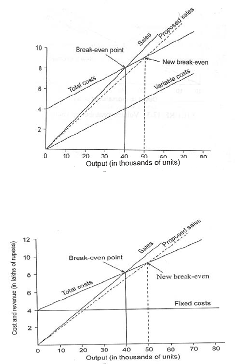
133
arithmetically. Contribution at 40,000 units is 40,000 x Rs. (20 - 10), i.e. Rs. 4, 00,000
which is equal to the fixed cost; and (vii) Revised revenue (revised on account of
reduction in selling price) shown by dotted line intersects total cost line at an output
of 50,000 units. The new break-even point is 50,000 units.
Graph 6.1: Break-even Chart
Graph 6.2: Break-even Chart with variable cost line
Detailed notes: (i) As in the conventional chart, the horizontal axis shows the units of
output and the vertical axis shows the cost and the revenue; (ii) The variable cost line
starts at nil and progresses evenly as the output increases. The conventional chart does
not show the variable cost line; (iii) Total cost line is parallel to variable cost line; the
gap between the two represents the fixed cost (Rs. 4, 00,000); and (iv) Revenue line
has been drawn in the same way as is drawn on conventional chart.
6.4.1 Volume contribution chart in Graph 6.3 is another way of presenting the

134
break-even point. Information in Example 6.3 has been used to draw the chart.
In this chart the contribution line starts at nil for nil output and progresses
evenly with increase in output. Break-even point is the point of intersection
between the contribution line and the fixed cost line. The advantage of this
method is that several lines at various selling prices and variable costs may be
drawn without the chart becoming too overburdened.
Graph 6.4 shows another method of depicting the break-even point. The horizontal
axis not only shows the sales volume in quantities, it shows the revenue (in rupee)
too. The chart clearly shows the profit or loss area, which starts at Rs. 4, 00,000 below
the break-even line (because Rs. 4, 00,000 being the fixed costs to be recovered to
break-even). Contribution line starts at nil with nil output and progresses evenly with
increase in sales. The point of intersection between the fixed cost line and the
Graph 6.3: Volume contribution chart
Graph 6.4: Volume contribution break-even chart.
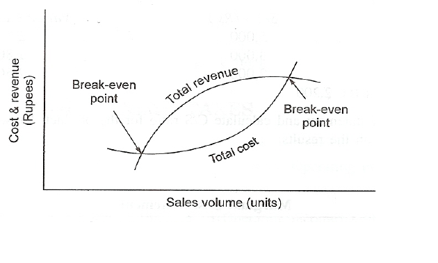
135
contribution line shows the break-even point.
The chart with reduction in selling price has to be drawn separately to avoid
confusion. (It will be a good practice for the reader to draw the chart with a reduced
selling price.) The fixed cost line and the revenue line will look the same as in Graph
6.4 except a change in the scale for revenue (Rs.) at the horizontal axis.
6.4.2 Limitation of break-even chart
In actual practice, Break-even charts are quite unlikely to resemble the chart shown
above because underlying assumptions in CVP analysis do not hold good in real-life
situations. The cost and revenue lines are not straight lines. They are rather curvilinear
and the chart might show more than one break-even point. Such a break-even chart
may look like the chart given in Graph 6.5.
6.4.3 Angle of incidence
This is the angle at which the sales line cuts the total cost line (Graphs 6.1 and 6.2). If
the angle is large, the firm (or product) is earning .profit at a high rate. If used in
conjunction with the margin of safety, it indicates an extremely favourable condition.
A small angle of incidence shows that although the firm (or the product) is making
profit, it is being achieved under less favorable conditions.
6.4.4 MULTI-PRODUCT PROFIT GRAPH
When a firm manufactures and sells more than one product of varying profitability; a
Graph 6.5: Curvilinear break- even chart.

136
CVP chart may be drawn to show the relative profitability of different products. This
graph is known as ‘Sequential profit graph’ or ‘Profit path chart’. The following steps
are involved in drawing the graph: (a) The C/S ratio is determined for different
products and products are arranged in order of the descending C/S ratio, i.e. the
product showing the highest C/S ratio is shown first and so on; (b) A statement is
prepared showing the cumulative sales and the cumulative profit; (c) Sales are plotted
on horizontal axis; (d) Fixed cost is plotted on vertical axis below the horizontal axis;
(e) Starting from the fixed cost point a profit path is drawn which terminates at the
profit point reached by the last product; (f) The end of the profit path is connected
with the fixed cost point. This line is called the total profit line; (g) The point of
intersection between the total profit line and the total sale line is called the break-even
point for a group of products.
Example 6.4: A manufacturing company produces three products: P, Q and R. The
following are the results for 2003.
Product Sales (Rs.) Variable cost (Rs.)
P 5000 2000
Q 3000 1800
R 2000 2500
Fixed Costs Rs. 2200
Prepare a marginal cost statement and calculate C/S ratio for the product. Draw a
profit-graph of products and comment on the results.
Solution:
Product P (Rs.) Q (Rs.) R (Rs.) Total (Rs.)
Sales 5,000 3,000 2,000 10,000
Variable cost (2,000) (1,800) (2,500) (6,300)
Contribution 3,000 1,200 (500) 3,700
C/S ratio 100
5000
3000 x 100
3000
1200 x 100
2000
500 x 100
10000
3700 x
= 60% = 40% = 25% = 37%
Break-even point = Fixed cost/ c/s ratio= 2,200/37%= Rs. 5,946.

137
Data for graph
Products are arranged in order of descending C/S ratio.
Product Sales
(Rs.) Cumulative
sales (Rs.) Contribution
(Rs.) Cumulative
contribution
(Rs.)
Fixed
cost
(Rs.)
Cumula
tive
profit
P 5,000 5,000 3,000 3,000 2,200 800
Q 3,000 8,000 1,200 4,200 2,200 2,000
R 2,000 10,000 (500) 3,700 2,200 1,500
Product R’s contribution is negative. Therefore, it should be discontinued, if possible.
The production of P, which has the highest contribution, should be increased.
However, non-cost factors should also be considered before taking the final decision.
6.4.5 Effects of Income Taxes
Generally, we know S-V-F= P or operating income,
After income tax effects, it will
Net income = Operating income - [(Operating income) x (Tax-rate)]
Or Net income = (Operating income) x (1 - Tax rate)
Or Operating income = Net Income/ (1 - Tax rate)
Thus, Revenue - Variable costs - Fixed costs = Net Income/ (1 - Tax rate)
Example 6.5: Football Shoe Company produces different products-all of which has
the same C/S ratio of 20%. The present sale is Rs. 60,000 per month and fixed cost is
Rs. 80,000 per annum. The following information is available from the budgeted
forecasts for the coming year:
Volume of sales No change
Increase in variable cost 5%
Estimated fixed cost Rs. 90,000
You are required to calculate: (a) The present yearly profit and (b) The percentage
increase required in selling prices during the forthcoming budget year in order to
maintain the existing level of profit.
Solution:
(a) The present yearly profit: Rs.
Sales for the current year 60,000 x 12 720000
Variable cost (80% of sales) Contribution (576000)
Fixed cost 144000

138
Present yearly profit (80000)
64000
(b) Percentage increase required in selling price:
Budgeted fixed cost 90000
Required profit 64000
Required contribution 154000
Variable cost (5, 76,000 + 5%) 604800
Required revenue 758800
Increase in price: increase
x%39.5
720000
100)720000758800( =
−
6.4.6 Break-even point and profit planning
Now, in the ensuing examples, we will explain the profit planning decisions.
Example 6.6: A company sells its product at Rs. 15 per unit. In a period, if it
produces and sells 8000 units, it incurs a loss of Rs. 5 per unit; if the volume is raised
to 20000 units, it earns a profit of Rs. 4 per units. Calculate break-even point both in
terms of rupees as well as units.
Solution:
Suppose, the contribution margin is c and fixed cost of F; therefore, contribution on
sale of 8000 units is 8000 c.
Thus,
8000 c = F-8000 x Rs. 5 or 8000c = F-Rs. 40000 (1)
Similarly, on sale of 20000 units, contribution is 20000 c
Thus,
20000c = F + 20000 x Rs. 4 or 20000c = F + Rs. 80000 (2)
Deducting Eq. (1) from Eq. (2) we get:
12000 c = Rs. 120000 or c + Rs. 10
Substituting c = Rs. 10 in Eq., (1) we get F = Rs. 120000
Break-even pointy in units = Rs. 120000/Rs. 10 units = 12000 units,
Break-even point in rupees = 1200 units x Rs. 15 = Rs. 180000.

139
Example 6.7: Indian Traders and Indian Corporation sell the same type of products
in same type of market. Their budgeted profit and loss account for the ending 2003
are as follows:
Indian Traders
Indian Corporation
Rs. Rs. Rs. Rs.
Sales 300000 300000
Variable cost 240000 200000
Fixed costs 30000 (270000) 70000 (270000)
Net Profit 30000 30000
You are required to:
a) Calculated the break-even points of each business; b) Calculated the sales-
volume at which each of the business will earn Rs. 10000 profit; and state which
business is likely to earn greater profit in condition of: Heavy demand for the profit;
and Low demand for the product. Give your reasons.
Solution:
(a) Break-even point
Indian Traders Indian Corporation
(Rs.) (Rs.)
Sales 300000 300000
Variable cost (240000) (200000)
Contribution 60000 100000
C/S ratio= 60000 x 100/300000= 20% 100000x100/ 3000000= 33.33%
Break-even point Rs. 30000 = Rs. 150000 Rs. 70000 = Rs. 21000
20% 33%
(b) Total contribution required:
Fixed costs 30000 70000
Profit required 10000 10000
40000 80000
Rs. 40000/20% Rs. 80000/33.33%
= Rs. 200000 = Rs. 240000
(c) Sales-volume at which both the firms would earn equal profit:
Let the sales volume be a
Profit of Indian Traders: a x 20 % - Rs. 30000 = 0.20 a – 30000
Profit for Indian Corporation: a x 33*1/3 % - Rs. 70000
The profit for both the firms being equal,
0.20a – a/3 – Rs. 30000 + Rs. 70000 = 0 or a = Rs. 300000

140
The C/S ratio of Indian Corporation at 33.33% is higher than that of Indian Traders at
20% Therefore, Indian Corporation will earn a higher profit if the sales volume
exceeds Rs. 300000 level. However, below that level profit for Indian Traders will be
higher. It may be concluded that Indian Corporation is likely to earn a higher profit
under conditions of heavy demand for the product. Similarly, Indian Traders is likely
to earn a higher profit under conditions of low demand for the product.
Example 6.8: Two manufacturing companies, which have the following operating
details, decide to merge.
Company 1
Company 2
Capacity utilization % 90 60
Sale (Rs. Lakh) 540 300
Variable costs (Rs. Lakh) 396 225
Fixed costs (Rs. Lakh) 80 50
Assuming that proposal is implemented, calculate:
(a) Break-even sales of the merged plant and the capacity
utilization at that stage
(b) Profitability of the merged plant at 80% capacity utilization
(c) Sales turnover of the merged plant to earn a profit of Rs. 75
lakh
(d) When the merged plant is working at a capacity to earn a profit
of Rs. 75 lakh, what percentage increase in selling price is required to
sustain as increase of 5 % in fixed overhead?
Solution: Operating data of the merged plant at 100% capacity:
Company 1 Company 2 Total merged
plant
Capacity 100% 100% 100%
(Rs. lakh) (Rs. lakh) (Rs. lakh)
Sales 54010.90 = 600 30010.60 = 500 1,100
Variable cost 396/0.90 = (440) 22510.60 = (375) (815)
Contribution 160 125 285
Fixed cost (80) (50) ( 130)
Profit 80 75 155
(a) Break-even point of the merged plant:

141
C/S ratio: Contribution x 100/Sales = 285 x 100/1100 = 25.91 %
Break-even point of the merged plant:
Fixed cost of the merged plant/ (c/s ratio) =130/25.91% = Rs. 501.74 lakh
Capacity utilization at break-even level:
= Sale value at break-even level/ Sale value at 100% capacity
= Rs. 501.74 lakh x 100/1100 = 45.6%
(b) Profitability of the merged plant at 80 % capacity utilization:
Sales at 80% capacity utilization = Rs. 1,100 lakh x 80% Rs. 880 lakh
Contribution at 80% capacity = Rs. 880 x 25.91 % Rs. 228 lakh
Fixed cost (Rs. 130 lakh)
Profit Rs. 98 Lakh
Profitability at 80% level 98 x 100/880 = 11.14%
(c) Sales to earn profit of Rs. 75,000:
Required contribution: (Rs. 75,000 + 1, 30,000) = Rs. 205 lakh
Sales turnover required: Required contribution
= Rs. 205 lakh = Rs. 781.20
C/S ratio 25:91 %
(d) Required percentage increase in selling price to sustain 5% increase in relaxed
cost:
Fixed cost at current level: Rs. 130 lakh
Increase in fixed cost 5% of Rs. 130 lakh Rs. 6.50 lakh
Hence, additional contribution required Rs. 6.50 lakh
Increase in selling price required =6.5 x 100/791.20 = 0.8215%
Example 6.9: X limited has been offered an order from A Ltd. for 10,000 units of
output @ Rs. 100 each which has a variable cost of Rs. 60 and will involve an outlay
of Rs. 60,000 to set-up jigs and dies. At the same time, there is another offer of B
Ltd., for 8,000 units of output at Rs. 110 each. Variable costs are estimated at Rs. 68
each and involve an outlay of Rs. 50,000 to set-up jigs and dies. Which offer should
the company accept?
Solution:
a) Contribution per units:
Price per unit Rs. 100 Rs. 110
Variable cost per unit (60) (68)
Contribution per unit Rs. 40 Rs. 42
b) Statement of profitability: A Ltd. B Ltd.

142
Output of units 10000 8000
Total contribution per unit Rs. 400000 Rs. 336000
Net profit (60000) (50000)
Net profit Rs. 340000 Rs. 286000
Profit from the offer of A Ltd., would be higher as compared to profit from the offer
of B Ltd. Therefore, the offer of A Ltd. should be accepted.
6.5 MARGINAL COSTING TECHNIQUES
Marginal costing technique assumes that fixed costs are given and only variable costs
and revenue can be influenced by short-term managerial actions. Therefore, in the
short-term, profit can be maximised by maximising total contribution, which is the
difference between total revenue and total variable costs. Managers decide the use of
scarce resources to maximise total contribution by evaluating alternative uses of
available resources. Underlying assumptions that fixed costs do not change with
change in the activity level and that there is a linear relationship between revenue and
variable costs, which do not hold good beyond the relevant range. Similarly, in
practice, it is difficult to segregate the total cost into fixed and variable elements
accurately. All these limit the reliability of marginal costing techniques. In spite of
these limitations, the marginal costing technique has emerged as an important
management tool.
6.5.1 PRODUCT MIX
6.5.1.1 Product Profitability
If the same facilities can be used to produce more than one product, contribution per
unit is taken as the profitability index for each product. The assumption is that there is
no limiting factor and there is no limit on the number of units of each product, which
can be produced and sold. In normal absorption costing, fixed costs are apportioned
equitably over products to determine each product's profitability. Apportionment is
based on the estimated usage of common resources by each product. The result may
143
be misleading because it may lead to the conclusion that products, which show a net
loss, should be discontinued.
6.5.1.2 Limiting Factor Analysis
Limiting factor or key factor is defined as anything which limits the activity of an
entity. An entity seeks to optimize the benefit it obtains from the limiting factor.
Examples are a shortage of supply of a resource and a restriction on sales at a
particular price. Limiting factors restrict the number of units that can be produced or
sold. Typical examples of limiting factors are: a) Sales demand in quantity, b) Sales
demand in value, c) A limit to availability of material, d) A limit to availability of a
particular grade of labour, e) A limit to machine capacity, and f) A shortage of
working capital. More than one limiting factor may operate at a particular point in
time. Under such a situation, the factor, which keeps the activity level at the
minimum, should be considered as the key factor. However, the impact of other
factors should also be considered in arriving at the final decision. Optimal utilization
of a scarce resource implies that all the available supply of that resource is used up.
Therefore, the contribution fund can be maximised by maximising the production and
sale of the product, which earns the highest contribution per unit of the limiting factor.
Thus, to determine the optimum production plan, the contribution per unit of the
limiting factor for each product is calculated and products are ranked in descending
order of contribution per unit of the limiting factor.
Example 6.10: A firm can produce two products A and B. The following are the cost
structures:
Product A (Rs.) Product B (Rs.)
Selling price per unit 20 22
Variable manufacturing cost per unit 5 6
Variable selling expenses per unit 3 2
Labour hours per unit 2 3

144
Total available labour hours are 1,200 per week. Assuming that the availability of
labour hours is the only limiting factor, determine which product should be
manufactured and sold.
Solution:
Contribution Statement
Product A Product B
(a) Selling price Rs.20 Rs.22
(b) Variable costs:
Manufacturing 5 6
Selling expenses 3
2
Total cost per unit Rs. 8
Rs. 8
(c) Contribution per unit (a - b) Rs. 12. Rs. 14
(d) Labour hours per unit 2 3
(e) Contribution per labour hour (c/d) Rs. 6 Rs. 4.67
If the firm utilizes all the available machine hours to produce product A, it will earn a
total contribution of Rs. 6 x 1,200, i.e. Rs. 7,200. On the other hand, if it uses the
available labour hours to produce product B, it will earn a total contribution of Rs.
4.67 x 1,200, i.e. Rs. 5,600. Therefore, product A should be manufactured. This can
also be verified as follows:
Product A Product B
(a) Available labour hour Rs. 1200 Rs. 1200
(b) Labour hours per unit 2 3
(c) Maximum output (a/b) 600 Units 400 Units
(d) Contribution per unit Rs. 12 Rs. 14
Total contribution (c x d) Rs. 7200 Rs. 5600
These calculations show that product A is more profitable than B. The same result
was reflected by the method of ranking products based on the contribution per labour
hour. Determination of the limiting factor poses problems because it changes rapidly.
A detailed analysis of the economic environment and the supply market of various
resources as well as internal factors are necessary to identify potential limiting factors.
Identification of limiting factors facilitates performance planning. The determination
145
of limiting factor is comparatively simple when only one product is produced or when
more than one product is produced using the same raw materials, labour and other
resources using the same process. However, it becomes very complex when a number
of products are manufactured from a variety of materials with different types of
labour using different types of machines or applying different processes. When there
is more than one limiting factor operating at a particular point in time, the profit
maximising budget could be determined by formulating and solving a linear
programming problem. This is beyond the scope of this book. However, simpler
decision models may be used when activities are restricted by only two limiting
factors.
6.5.2 MAKE OR BUY DECISION
If no limiting factor is in operation, the decision to buy or to manufacture a product
rests on whether the bought-out price of an article is lower than its marginal cost. The
fixed cost is irrelevant for our decision because fixed cost will not change as a result
of buying the product/component from outside. If the bought-out price of an article is
lower than its marginal cost, it will be profitable to buy the article from outside in all
circumstances. The firm will save marginal cost and will spend lower than the
marginal cost to buy the article. If the bought-out price is higher than the marginal
cost, the total cost of production will increase, if the firm decides to buy the article
from outside. Therefore, if it has a choice, it will buy the article for which the
difference between the bought-out price and the marginal cost is the lowest among
article under consideration. If a limiting factor is in operation, the excess of bought-
out price over marginal cost per unit of the limiting factor is to be considered. The
article having the lowest excess of bought out price over its marginal cost per unit of
the limiting factor will be selected for buying out from outside.

146
Example 6.11: The cost of manufacturing and bought-out prices of four articles is as
follows:
Article A B C D
Production cost per article:
Marginal cost Rs. 10.00 Rs. 12.00 Rs. 15.00 Rs. 15.00
Fixed cost 2.00 4.00 5.00 15.00
Total cost 12.00 16.00 20.00 30.00
Production per-man hour 0.25 0.20 0.20 0.33
Production per machine hour 1.00 0.50 0.25 0.20
Bought-out price Rs. 9.00 Rs. 17.00 Rs. 22.00 Rs. 26.00
Rank the products in the order of your preference for buying them from outside (a)
when there is no limiting factor; (b) if man-hour is the limiting factor, (c) if machine
capacity is the limiting factor.
Solution:
Articles A B C D
Bought-out price per unit Rs. 9.00 Rs. 17.00 Rs. 22.00 Rs. 26.00
Marginal cost (per unit) of
production 10.00 12.00 15.00 15.00
Excess of bought-out price
over
marginal cost per article
-1.00 5.00 7.00 11.00
Excess per man-hour -1.00 x 0.25
= - 0.25 5.00 x 0.20
= 1.00 7.00 x 0.20
= 1.40 11.00 x 0.33
= 3.63
Excess per machine hour -1.00 x 1
= -1.00 5.00 x 0.50
= 2.50 7.00 x 0.25
= 1.75 11.00 x 0.20
= 2.20
In case of article A, the bought-out price is lower than the marginal cost, hence to
purchase A from outside is always profitable.
Ranking of products in order of preference for buying out:
(a) When there is no limiting factor 1st A, 2nd B, 3rd C, 4th D
(b) When man-power is the limiting factor 1st A, 2nd B, 3rd C, 4th D
(c) When machine capacity is the limiting factor 1st A, 2nd C, 3rd D, 4th B
6.5.3 DECISION ON METHODS OF MANUFACTURING
Marginal costing technique can be used to choose from alternative methods of
manufacturing. The method, which generates the highest contribution, is the most
desirable method. The decision, therefore, rests on the contribution per unit or the
contribution per unit of the limiting factor, if a limiting factor is identified.

147
Example 6.12: An undertaking is producing an article, the selling price of which is
Rs. 20 per unit. A decision has to be taken whether:
(a) to produce by hand (Method A); or
(b) to produce by machine, one operator to one machine (Method B); or
(c) to produce by machine, one operator to two machines (Method C); or
(d) to produce by machine, one operator to three machines (Method D).
The cost of manufacturing the article by different methods is as follows:
Method A B C D
Cost per article (Rs.):
Material 1 unit 5.00 5.00 5.00 5.00
Direct labour @ Rs. 3 per man-hour 5.00 3.00 1.70 1.50
Variable overhead @ Rs. 2 per man-hour 3.30 2.00 1.10 1.00
Variable overhead @ Re. 1 per machine-
Hour - 1.00 1.10 1.50
Total marginal cost 13.30 11.00 8.90 9.00
Fixed overhead @ Re. 1 per man-hour 1.70 1.00 0.90 0.50
Fixed overhead @ Rs. 6 per machine-
Hour - 6.00 6.60 9.00
Total cost 15.00 18.00 16.40 18.50
Production per man-hour 0.60 1.00 1.75 2.00
Production per machine-hour - 1.00 0.875 0.66
Solution:
Method A B C D
Selling prices per unit (Rs.) 20.00 20.00 20.00 20.00
Marginal cost per unit (Rs.) (13.30) (11.00) (8.90) (9.00)
Contribution per unit 6.70 9.00 11.10 11.00
Contribution per unit of material
6.70/1
= Rs. 6.70 9.00/1
= Rs. 9.00 11.10/1
= Rs. 11.00 11.00/1
= Rs. 11.00
Contribution per man hour
6.70 x 0.6
= Rs. 4.20 9.00 x 1
= Rs. 9.00 11.10 x 1.75
= Rs. 19.40 11.00 x 2
= Rs. 22.00
Contribution per machine hour
9.00 x 1
= Rs. 9.00 11.10 x 0.875
= Rs. 9.70 11.00 x 0.66
= Rs. 7.30
If there is no limiting factor, Method C should be selected as it generates the highest
contribution per unit. If a limiting factor is in operation, the method to be adopted
should be the one, which gives the highest contribution per unit of the limiting factor.
Thus,
(a) If material is the limiting factor, method C should be adopted.
148
(b) If man-power is the limiting factor, method D should be adopted.
(c) If machine capacity is the limiting factor, method C should be adopted.
6.5.4 SHUTTING DOWN DECISIONS
Marginal costing technique can be used in deciding whether to discontinue a section
of the business. If we assume that discontinuance will not influence the total fixed
costs of the firm, the decision will hinge on whether the particular section of the
business is contributing towards fixed overheads. Closure of an activity, which
generates positive contribution, reduces the current operating profit or increases the
operating loss. In certain situations, a part of the fixed cost is avoided by temporary
closure. In such a situation, if avoidable fixed cost is higher than expected
contribution, the business segment should be closed.
Example 6.13: A company making a single product has a factory at Howrah (near
Kolkata) and distributes its product through three depots situated in Kolkata, Kanpur
and Chennai. It is estimated that during the year 1, 00,000 units will be manufactured
and sold at a price of Rs. 30 per unit, the sales being spread is as follows:
Kolkata 70,000 units
Kanpur 20,000 units
Chennai 10,000 units
Standard costs of production are:
Direct materials Rs. 6 per unit
Direct wages Rs. 5 per unit
Factory variable overheads 160% of direct wages
Factory fixed overheads Rs. 6, 00,000 per annum
The cost of selling and distribution incurred by the depots are:
Calcutta Kanpur Chennai
Fixed Cost per annum 100000 70,000 30000
Variable cost (% of sales value) 10% 8% 7%
The budget for the business prepared from these figures caused the management to
consider the closure of Kanpur and/or Chennai depots. If this is done, all sales in these
areas will be lost, but sales from the Kolkata depot will remain unaffected.
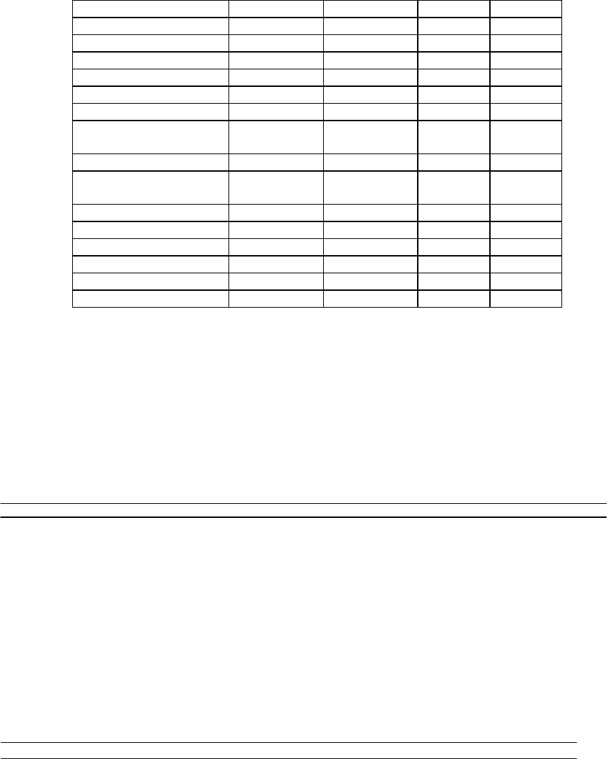
149
You are required to
(a) Prepare a budget for the business from the figures provided; and
(b) Advise the management on the desirability of closing down Kanpur and Chennai
depots.
Solution:
This presentation shows that operations of Kanpur and Chennai depots have resulted
in losses and this leads the management to consider their closure. An alternative
presentation using the marginal cost approach helps the management to take correct
decision.
Kolkata Kanpur Chennai Total
Sales 2100 600 300 3000
Variable costs of production
Direct materials 600
Direct wages 500
Variable factory overheads 800
Allocated pro-rata to units 1330 380 190 1900
770 220 110 1,100
Variable costs of selling and distribution 210 48 21 279
Contribution to all fixed expenses 560 172 89 821
Fixed costs of selling and distribution assuming 100 70 30 200
that they are specific to each depot
Contribution to fixed factory overheads 460 102 59 621
Fixed factory overheads 600
Net profit. 21
Calcutta Kanpur Chennai Total
Unit 70,000 20,000 10.000 100,000
Sales Rs. '000 Rs. '000 Rs. '000 Rs. '000
2,100 600 300 3000
Production Cost :
Direct Material 600
Direct Wages 500
Factor Variable
overheads 800
Factory fixed overheads 600
Allocated pro-rata to
units 1,750 500 250 2500
Gross Profit 350 100 50 500
Selling and distribution
Variable 210 48 21 279
Fixed 100 70 30 200
Local costs 310 118 51 479
Net Profit/(loss) 40 (18) (1) 21
150
This presentation shows that sales at Kanpur and Chennai depots make contribution of
Rs. 1, 02,000 and Rs. 59,000 respectively, towards fixed factory overheads.
Therefore, none of those two depots should be closed down. In the above
presentation, it is assumed that fixed selling and distribution costs could be avoided
by closing those depots. This may not happen in the short term.
6.5.5 MARGINAL COST AND PRODUCT PRICING
A long-term pricing policy should aim to recover more than the 'full cost' to ensure a
reasonable return on capital employed. A firm cannot survive if it has to sell its
products continuously below 'full cost'. Marginal cost may be used as a basis for
short-term pricing decisions. Usually, marginal cost is used to determine prices for
non-repetitive orders under difficult business conditions or to use spare capacity when
acceptance of lower contributions and profit margins may be necessary. When
capacity is unused, acceptance of an order with lower contribution helps partial
recovery of the fixed cost. Factors to be considered in fixing selling prices when
demand is below normal are the amount and the rate of contribution which the
proposed selling price would yield; probability of securing an order with higher
contribution during the period of execution of the order; proposed concession, when
compared with the normal selling price on full cost basis; probable adverse effects on
future sales. When one or more resources are scarce, (e.g. material is scarce), the first
consideration must be to reserve the same for orders that would yield the highest
contribution per unit of the scarce resource (the limiting factor). A decision to sell at a
lower price might also have an adverse effect on the firm's general level of selling
prices in its established market. This aspect should also be carefully examined before
accepting an order with contribution lower than the normal contribution.

151
Other factors, which strongly justify acceptance of an order with lower contribution at
the time adverse trade situations, are to: (a) hold together the skilled labour force; (b)
keep the plant and machinery in operation and the workers busy; (c) utilize materials
already received; (d) avoid costs involved in the closing and re-opening of the plant;
(e) maintain the sales of complementary products at a satisfactory level; and (f)
maintain position in established markets to avoid additional sales promotion expenses
in reestablishing the markets.
Selling below full cost prices, even under a normal situation, may be adopted in order
to: (a) introduce a new product, (b) execute an order in a special market segment (say,
defense supply) which is immune from other market segments; (c) expand the export
market; and (d) dispose of a product which deteriorates fast.
Example 6.14: The Everest Snow company manufactures and sells direct to
consumers 10,000 jars of 'Everest Snow' per month at Rs. 1.25 per jar. The company's
normal production capacity is 20,000 jars of snow per month. An analysis of cost for
10,000 jars is given below:
Direct material Rs. 1000
Direct labour 2475
Power 140
Miscellaneous supplies 430
Jars 600
Fixed expenses of manufacturing, selling and administration 7955
Total Rs. 12600
The company has received an offer for the export, under a different brand name for
1, 20,000 jars of snow at 10,000 jars per month at 75 paise a jar. Write a short report
on the advisability or otherwise of accepting the offer.
Solution:
Statement of Contribution from the Export Order
Selling price per unit Rs. 0.7500
Variable cost per unit:
Direct material Rs. 1,000/10,000 0.1000

152
Direct labour Rs. 2,475/10,000 0.2475
Power Rs. 140/10,000 0.0140
Misc. supplies Rs. 430/10,000 0.0430
Jars Rs. 600/10,000 0.0600 (0.4645)
Contribution margin per unit Rs. 2855
Contribution per month: Rs. 0.2855 x 10,000 Rs. 2855
Acceptance of the export order would result in incremental contribution of Rs. 2,855
per month. The following statement reveals monthly profit, with and without
acceptance of order.
Present position Proposed offer Total
(10,000 jars) (10000 jars) (20000 jars)
Sale Value Rs. 12,500 7500 20000
Variable cost of sales @ Rs. 0.4645 (4,645) (4,645) (9290)
Contribution 7,855 2855 10710
Fixed Cost (7,955) - (7955)
Profit -100 2855 2755
It is advisable to accept the order provided:
(a) interest on incremental working capital would be lower than the total contribution
from the export order;
(b) acceptance of the export order with lower contribution would not adversely affect
the price in home-maker or the future sales;
(c) there is no possibility for dumping, i.e. re-export by the supplier; and
(d) there is no possibility of securing an order with higher contribution during the
period of execution of the order.
Example 6.15: AB Ltd. manufactures three products X, Y, and Z. Standard selling
process and costs have been established for 2003 as follows: .
X Y Z
Selling price per unit Rs. 28 Rs. 60 Rs. 125
Direct materials per unit 8 15 20
Direct wages per unit 10 20 50
Variable overheads per unit 5 10 25

153
Direct wages are paid at the rate of Rs. 2 per hour in each case. Fixed overheads are
budgeted at Rs. 25,000 for the coming year.. In the short run, the company cannot
increase its direct labour strength and as a result, only 35,000 direct labour hours will
be available in the coming year. The company has commitments to produce 500 units
of each product. It has been suggested that after meeting the minimum requirements
for X, Y and Z, the balance of available direct labour hours should be used to produce
product Z. You are required:
A) To prepare an income statement showing the expected results if the proposal is
adopted.
B) Comment on the statement you have produced in (a) and prepare an income
statement for any alternative policy, which you consider would be more
profitable.
C) Basing your calculations on your suggestion in (b), show the company's break-
even point in terms of units and sales value.
D) Show the sale value which is required to produce an after tax return of 10% on
capital employed of Rs. 1, 00,000 assuming tax rate of 50%.
Solution:
(a) Income Statement Showing Results if the Proposal is Adopted (Rs. '000)
Product X Product Y Product Z Total
1. Sales value 14.00 30.00 137.50 181.50
2. Variable costs:
Direct materials 4.00 7.50 22.00 33.50
Direct wages 5.00 10.00 55.00 70.00
Variable overheads 2.50 5.00 27.50 35.00
Total 11.50 22.50 104.50 138.50
3. Contribution fund (1 - 2) 2.50 7.50 33.00 43.00
4. Fixed overheads 25.00
5. Operating profit (3 - 4) 18.00
Thus, the operating profit will be Rs. 18,000.

154
Notes: (i) Total available direct labour hours 35,000
Labour hours to be utilized to meet commitments:
(500 x 5 + 500 x 10 + 500 x 25) 20,000
Balance hours available 15,000
(ii) Additional units of Z to be produced 15,000/25, i.e. 600 units
Thus, total production of Z will be (500 + 600), i.e. 1,100 units
(iii) Required direct labour hours for each unit of production of
X: 10/12, i.e. 5 hours, Y: 20/2, i.e. 10 hours and Z: 50/2, i.e. 25 hours.
(b) Profitability Statement
Product X Product Y Product Z
1. Selling price Rs.28 Rs.60 Rs. 125
2. Variable costs per unit:
Direct materials 8 15 20
Direct wages 10 20 50
Variable overheads 5 10 25
Total Rs.23 Rs.45 Rs.95
3. Contribution per unit (1 - 2) Rs. 5 Rs.15 Rs.30
4. Required labour hours per unit 5 10 25
5. Contribution per labour hour (3/4) Re. 1.00 Rs. 1.50 Rs. 1.20
6. Ranking III I II
Availability of labour hours being limited, AB Ltd. should produce as many unit of T
as possible. There being no restriction on the units of Y that can be sold, available
labour hours, after meeting the commitments for products X and Z should be allocated
to Y. Thus, optimal product mix is:
Product Units to be produced Allocated Labour hours
X 500 2500
Y 2,500 20000 (Balancing figure)
Z 500 12500
35,000
Income Statement with the above Alternative
Products Total

155
X Y Z (Rs. ‘000)
Contribution 2.5 30.00 15.00 47.50
Fixed costs 25.00
Operating profit (1 - 2) 22.50
(c) Break-even point in terms of units and sales
Contribution from committed production and sales:
Production X: 500 x Rs. 05.00 Rs. 2,500
Production Y: 500 x Rs. 15.00 7,500
Production Z: 500 x Rs. 30.00 15,000
Rs. 25,000
Fixed cost being Rs. 25,000, break-even sales of AB Ltd. is sales of 500 units of each
of the three products X, Y and Z. Break-even sales in terms of value is (500 x 28 +
500 x 60 + 500 x 125), i.e. Rs. 1,06,500.
(d) Sales value to earn a post-tax return of 10% on capital employed
Required return 10% of Rs. 1,00,000 i.e. Rs. 10,000
Required operating profit = 20,000 Rs.
50.0
10,000 Rs.
0.50)(1
10,000 Rs.
ratetax (1
return Required ==
−
=
−
Committed sales will earn contribution enough to meet fixed costs. Therefore, to earn
an operating profit of Rs. 20,000 additional units of Y is to be sold to earn a
contribution of Rs. 20,000. Thus, the total number of units of Y to be sold is (500 +
Rs. 20,000/15) i.e. 1,833.33 or 1,834 units.
Thus, total sale value is
X: 500 x Rs. 28 = Rs. 14,000
Y: 1,834 x Rs. 60 = Rs. 1,10,040
Z: 500 x Rs. 125 = Rs. 62,500
Total = Rs. 1, 86,540

156
Example 6.16: The costs per unit of the three products A, Band C of a company are
given below:
Product A Product B Product C
Direct material Rs.20 Rs.16 Rs. 18
Direct labour 12 14 12
Variable expenses 8 10 6
Fixed expenses 6 6 4
46 46 40
Profit 18 14 12
Selling price 64 60 52
No. of units produced 10,000 5,000 8,000
Production arrangements are such that if one product is given up the production of the
other can be raised by 50%. The directors propose that C should be given up because
the contribution from the product is the lowest. Present suitable analysis of the data
indicating whether the proposal should be accepted.
Solution:
Statement Showing Contribution per Unit
Product A Product B Product C
Selling price per unit Rs. 64 Rs.60 Rs.52
Variable costs: Direct material Rs.20 Rs. 16 Rs.18
Direct labour 12 14 12
Variable expenses 8 10 6
Rs.40 Rs.40 Rs.36
Contribution per unit Rs.24 Rs.20 Rs. 16
In the absence of any limiting factor, the company should produce as many units of A
as possible. In case a limiting factor is in operation, contribution per unit of the
limiting factor should be used to measure profitability. In this particular case, the
limiting factor is not clearly spelt out, although a restrictive condition is specified. It
indicates the discontinuance of a product, which will result in the increase in
production of other products by 50%. In this situation, a decision to abandon a
product line should consider incremental contribution from each of the three
alternatives, giving up either product A or product B or product C.
Alternative I- Discontinue product A

157
Additional contribution:
Product B: 0.5 x 5,000 x Rs. 20 = Rs. 50,000
Product C: 0.5 x 8,000 x Rs. 16 = Rs. 64,000 Rs. 1,14,000
Loss of contribution A: 10,000 x Rs. 24 (Rs. 2, 40,000)
Incremental contribution (Rs. 1, 26,000)
Alternative II-Discontinue product B
Additional contribution:
Product A: 0.5 x 10,000 x Rs. 24 = Rs. 1,20,000
C: 0.5 x 8,000 x Rs. 16 = Rs. 64,000 Rs.1, 84,000
Loss of contribution B: 5,000 x Rs. 20 (1, 00,000)
Incremental contribution Rs. 84,000
Alternative III-Discontinue product C
Additional contribution:
Product A: 0.5 x 10,000 x Rs. 24 = Rs. 1,20,000
B: 0.5 x 5,000 x Rs. 20 = Rs. 50,000 Rs. 1, 70,000
Loss of contribution A: 8,000 x Rs. 16 (1, 28,000)
Incremental contribution Rs. 42,000
Incremental contribution is highest from alternative II (discontinuance of product B),
and therefore, the decision to discontinue product C is sub-optimal. Product B should
be discontinued for maximising profit and proposal to discontinue product C should
not be accepted.
6.6 SUMMARY
Cost-volume-profit (CVP) analysis is the study of the effect on future profit of
changes in fixed cost, variable cost, selling price, sales quantity and sales mix. CVP
analysis assumes that the cost structure and the relationships between fixed costs,
158
variable cost and selling price will remain valid during the period under consideration.
Therefore, the analysis produces useful results for decisions within the 'relevant range'
and the ‘relevant period’. Moreover, there are certain simplistic assumptions
underlying the CVP analysis which limit the precision and reliability of the result of
the analysis. CVP analysis uses a simple equation, which captures the relationships
between different variables. Graphical methods are also used for the study. A break-
even chart represents the relationships between different variables. Managers use
different variations of the simple breakeven chart.
In this chapter, we have discussed the use of cost information for tactical decisions.
Tactical decisions are short-term decisions that aim at maximizing operating profit,
with available facilities. Therefore, usually such decisions take into consideration
marginal costs only. However, sometimes short-term decision influence fixed costs,
e.g. additional advertising expenses. Thus, incremental fixed expenses cannot be
ignored. Marginal costing technique is used to determine optimal product-mix. A firm
maximizes operating profit by producing products, which contribute highest towards
fixed costs and profit. Therefore, contribution per unit of the limiting factor is used as
profitability index. The limiting factor is the scarce resource or any other factor,
which restricts the activity level. Often other restrictive conditions determine the
optimal product-mix. Marginal costing technique is used to decide whether a
component is to be manufactured or to be purchased from outside. If spare capacity is
available, the product should be manufactured only if variable-manufacturing cost is
lower than purchase price. If spare capacity is not available, manufacturing decision
results in the discontinuance of another product. Therefore, loss of contribution due to
discontinuance should be added to the costs of manufacturing and the total should be
compared with the purchase price. If the firm has no choice but to purchase some
159
components from outside, it decides in favour of the component, manufacturing of
which generates savings lowest among the alternative products. For short-term
decisions on methods of manufacturing or temporary shut down of plant/ business,
managers use marginal costing technique-considerations are similar to those discussed
above.
6.7 SELF-TEST QUESTIONS
1. Define 'marginal costing'. How are variable costs and fixed costs treated in
marginal costing? Give a journal entry for overhead accounts under marginal
costing.
2. What are the important areas of management decisions opened up by the
application of marginal costing technique? Answer briefly and to the point.
3. Explain CVP analysis and Break-even-point analysis.
4. In a purely competitive market, 10,000 pocket transistors can be manufactured
and sold, and a certain profit is generated. It is estimated that 2,000 pocket
transistors need to be manufactured and sold in a monopoly market to earn the
same profit. Profit under both the conditions is targeted at Rs. 2, 00,000. The
variable cost per transistor is Rs. 100 and the total fixed cost is Rs. 37,000. You
are required to find out the unit selling prices both under monopoly and
competitive conditions. (Ans: A: Rs. 218.50, B: Rs. 123.70).
5. Y Company has just been incorporated and plans to produce a product that will
sell for Rs. 10 per unit. Preliminary market survey shows that demand will be
around 10,000 units per year. The company has the choice of buying one of the
two machines, each of which has a capacity of 10,000 units per year. Machine A
would have fixed costs of Rs. 30,000 per year and would yield a profit of Rs.
30,000 per year on the sale of 10,000 units. Machine B would have fixed costs of

160
Rs. 18,000 per year and would yield a profit of Rs. 22,000 per year on the sale of
10,000 units. Variable costs behave linearly for both machines. Required:
(a) Break-even sales for each machine.
(b) Sales level where both machines are equally profitable.
(c) Range of sale where one machine is more profitable than the other.
(Ans.: (a) 5000 units, 4500 units; (b) 6,000 units; (c) As the C/S ratio in the case
of Machine A (60%) is higher than the C/S ratio in the case of Machine B (40%),
profit in the case of Machine A increases at a faster pace as compared to the
increase in profit in the case of Machine B beyond the break-even point. From the
fact that at the output level of 6,000 units both machines are equally profitable, it
is obvious that below 6,000 units output level, profit from Machine B is higher as
compared to profit from Machine A and beyond 6,000 units output level, profit
from machine A is more).
6. A company has an opening stock of 6,000 units of output. The production planned
for the current period is 24,000 units and expected sales for the current period
amounted to 28,000 units. The selling price per unit of output is Rs. 10. Variable
cost per unit is expected to be Rs. 6 per unit while it was only Rs. 5 per unit
during the previous period. What is the break-even volume for the current period
if the total fixed costs for the current period are Rs. 86,000? Assume that the first-
in-first-out system is followed. (Ans.: 20,000 units).
7. (Closure of product line) A Ltd. manufactures three products and the cost
particulars for a year are as follows:
Product X (Rs.) Product Y(Rs.) Product Z
Sales 2, 00,000 4, 00,000 2,50,000
Material 1, 00,000 1, 50,000 1, 25,000
Labour cost 30,000 50,000 40,000

161
Variable overheads 10,000 20,000 25,000
Fixed Overheads 35,000 50,000 25,000
The company imports one of the raw materials, which is used in the manufacture
of all products. The consumption of material is as follows:
X - 2,000 kgs.
Y - 5,000 kgs.
Z - 3,000 kgs.
There is a restriction on the import of the material. The management is planning to
close down one of the lines of product and utilize the material for other two lines
to improve the profitability. As the secretary of the company, prepare a report for
the closure of one line for improving the profitability.
(Ans.: Contribution per kg of imported material X: Rs. 30, Y: Rs. 36, Z: Rs. 20).
8. (Product-mix) Mega Corporation manufactures and sells three products to the
automobile industry. All the products must pass through a machining process, the
capacity of which is limited to 20,000 hours per annum, both by equipment design
and government regulation. The following additional information is available:
Product X (Rs.) Product Y (Rs.) Product Z
Selling price Rs./ unit 1,900 2,400 4,000
Variable cost Rs./ unit 700 1200 2800
Machine requirement hrs./ unit 3 2 1
Maximum possible sales units10,000 2,000 1,000
Required: A statement showing the best possible production mix which would
provide the maximum profit for Mega Corporation, together with supporting
work.
(Ans.: Product-mix X: 5,000 units, Y: 2,000 units, Z: 1,000 units. Total
contribution = Rs. 96,000).
8. (Acceptance of export order) A company produces a single product which is sold
by it presently in the domestic market at Rs. 75 per unit. The present production
and sales is 40,000 units per month representing 50% of the capacity available.
The cost data of the product are as under:
Variable cost per unit Rs. 50
Fixed cost per month Rs. 10 lakh.
162
With a view to improve the profitability, the management has three proposals on
hand as under: (a) to accept an export supply order for 30,000 units per month at a
reduced price of Rs. 60 per unit, incurring additional variable costs of Rs. 5 per
unit towards export packing, duties etc.; (b) to increase the domestic market sales
by selling to a domestic chain stores 30,000 units at Rs. 55 per unit, retaining the
existing sales at the existing price; (c) to reduce the selling price for the increased
domestic sales as advised by the sales department as under:
Reduce selling price per unit by Rs. Increase in sales expected (in units)
5 10,000
8 30,000
11 35,000
Prepare a table to present the results of the above proposals and give your
comments and advise on the proposals.
(Ans.: Operating profits: Current Nil, Proposal (a) Rs. 1,50,000; Proposal (b) Rs.
1,50,000, Proposal (c) Selling price 70 Rs. Nil, S.P. Rs. 67, Rs. 1, 90,000, S.P. Rs.
64, Rs.50, 000).
6.8 SUGGESTED READINGS
1. Ashish K. Bhattacharya, Principles and Practices of Cost Accounting (3rd.),
New Delhi: Prentice Hall of India Private Limited, 2004.
2. Charles T. Horngren, Cost Accounting, A Managerial Emphasis, Prentice Hall
Inc., 1973.
3. D. T. Decoster and E. L. Schafer, Management Accounting, New York: John
Willey and Sons, 1979.
4. John G. Blocker and Wettmer W. Keith, Cost Accounting, New Delhi: Tata
McGraw Publishing Co. Ltd., 1976.
5. R. K. Sharma and Shashi K. Gupta, Management Accounting-Principles and
Practice (7th.), New Delhi: Kalyani Publishers, 1996.

163
Objective: The present lesson explains the various facets of a standard costing system.
LWSSON STRUCTURE
7.1 Introduction
7.2 Meaning of Standard Cost And Standard Costing
7.3 Steps involved in Standard Costing
7.4 Standard Costing Vs. Budgetary Control
7.5 Standard Costs and Estimated Costs
7.6 Advantages of Standard Costing
7.7 Limitations of Standard Costing
7.8 Preliminaries for Establishing Standard Costing System
7.9 Analysis of Variances
7.10 Accounting Treatment of Variances
7.11 Summary
7.12 Self-Test Questions
7.13 Suggested Readings
7.1 INTRODUCTION
The basic function of management accounting is to facilitate the managerial control in
a business unit or organisation. Management control is the process of evaluating
performance and applying corrected measures, if required, so that performance takes
place according to plans. The major aspect of managerial control is cost control. And
the ‘Standard Costing’ is that technique which helps management to control costs and
COURSE: MANAGEMENT ACCOUNTING
COURSE CODE: MC-105 AUTHOR: SURINDER SINGH KUNDU
LESSON: 07 VETTER: PROF. H. L. VERMA
STANDARD COSTING
164
business operations. It aims at eliminating wastes and increasing efficiency in
performance through setting up standards or formulating different cost plans.
7.2 MEANING OF STANDARD COST AND STANDARD COSTING
The word ‘standard’ means a benchmark or gauge. The ‘standard cost’
is a predetermined cost which determines in advance what each
product or service should cost under given circumstances. Backer and
Jacobsen define “Standard cost is the amount the firm thinks a
product or the operation of a process for a period of time should cost,
based upon certain assumed conditions of efficiency, economic
conditions and other factors”. Chartered Institute of Management
Accountants, London defines standard cost as “a predetermined cost
which is calculated from management’s standards of efficient
operation and the relevant necessary expenditure”. They are the
predetermined costs based on technical estimate of material, labour
and overhead for a selected period of time and for a prescribed set of
working conditions.
The technique of using standard costs for the purposes of cost control
is known as standard costing. Brown and Howard define “standard
costing is a technique of cost accounting which compares the
standard cost of each product or service with actual cost to determine
the efficiency of the operation so that any remedial action may be
taken immediately”. The terminology of Cost Accountancy defines
standard costing as “the preparation and use of standard costs, their
comparison with actual costs, and the analysis of variance to their
causes, and points of incidence”. The London Institute of Cost and
Works Accountants define it as "An estimate cost, prepared in
advance of production or supply correlating a technical specification of
material and labour to the price and wage rates estimated for a
selected period of time, with an addition of the apportionment of
overheads expenses estimated for the same period within a prescribed
set of working conditions”. Further, it is a system of cost accounting,
165
which is designed to find out how much should be the cost of a
product under the existing conditions. The actual cost can be
ascertained only when production is undertaken. The predetermined
cost is compared to the actual cost and a variance between the two
enables the management to take necessary corrective measures.
7.3 STEPS INVOLVED IN STANDARD COSTING
The technique of standard costing involves the determination of cost before occurring.
The standard cost is based on technical information after considering the impact of
current conditions. With the change in condition, the cost also can be modified so as
to make it more realistic. The standard cost is divided into standards for materials,
labour and overheads. The actual cost is recorded when incurred. The standard cost is
compared to the actual cost. The difference between the two costs is known as
variance. The variances are calculated element wise. The management can take
corrective measures to set the things right on the basis of different variances.
The basic purpose of standard costing is to determine efficiency or inefficiency in
manufacturing a particular product. This will be possible only if both standard costs
and actual costs are given side by side. Though standard costing system will be useful
for all types of commercial and industrial undertakings but it will be more useful in
those undertakings where production is standardized. It will be of less use in job
costing system because every job has different specifications and it will' be difficult to
determine standard costs for every job.
7.4 STANDARD COSTING Vs. BUDGETARY CONTROL
In budgetary control, budgets are used as a means of planning and control. The targets
of various segments are set in advance and actual performance is compared with
predetermined objects. In this way management can assess the performance of
different departments. On the other hand, standard costing also set standards and
enables to determine efficiency on the basis of standards and actual performance.
166
Budgetary control is essential to determine standard costs, whereas, the standard
costing system is necessary for planning budgets. In budgetary control the budgets are
prepared for the concern as a whole whereas in standard costing the standards are set
for producing a product or for providing a service. In standard costing, unit concept is
used while in budgetary control total concept is used. The budgets are fixed on the
basis of past records and future expectations. Standard costs are fixed on the basis of
technical information. Standard costs are planned costs and these are expected in
future. As far as scope is concerned, in case of budgetary control it is much wider than
standard costing. Budgets are prepared for incomes, expenditures and other functions
of the departments such as purchase, sale, production, finance and personnel
department. In contrary, standards are set up for expenditures only and, therefore, for
manufacturing departments standards are set for different elements of cost i.e.,
material, labour and overheads.
Further, in budgetary control, the targets of expenditure are set and these targets
cannot be exceeded. In this system the emphasis is on keeping the expenditures within
the budgeted figures. In standard costing the standards are set and an attempt is made
to achieve these standards. The emphasis is on achieving the standards. Actual costs
may be more than the standard costs and there can be no such thing in budgetary
control. The budgetary control system can be applied partly or wholly. Budgets may
be prepared for some departments and may not be prepared for all the departments. If
a concern is interested in preparing production budget only, it is free to do so.
Standard costing cannot be used partially; it will have to be used wholly. The
standards will have to be set for all elements of cost. In fact, the systems operate in
two different fields and both are complimentary in nature.
7.5 STANDARD COSTS AND ESTIMATED COSTS
167
The standard costs and estimated costs both are used to determine price in advance.
The purpose of both of them is to control cost. They follow the same accounting
principles. Despite similarities, they differ in terms of objects and purpose. Estimated
costs are based on historical accounting. It is an estimate of what the cost will be. It is
a cost of guesswork or reasonable estimate for the costs in future. On the other hand
standard costs are based on scientific analysis and engineering studies. Standard
costing determines what the cost should be. Standard costs are used as a device for
measuring efficiency. The standards are predetermined and a comparison of standards
with actual costs enables to determine the efficiency of the concern. Estimated costs
cannot be used to determine efficiency. It only determines the expected costs. An
effort is made that estimated cost should almost be near to actual costs. The purpose
of determining estimated costs is to find out selling price in advance to take a decision
whether to produce or to make and also to prepare financial budgets. Estimated costs
do not serve the purpose of cost control. On the other hand standard costs are helpful
in cost control. The analysis of variance enables to take corrective measures, if
necessary. Standard costs are not easily changed. The standards are set in such a way
that small changes in conditions do not require a change in standards. Estimated costs
are revised with the change in conditions. They are made more realistic by
incorporating changes in prices. Standard costs are more static than estimated costs.
Estimated costs are used by the concern using historical costing. Standard costing is
used by those concerns which use standard costing system. Standard costing is a part
of cost accounting process while estimated costs are statistical in nature and as such
they may not become a part of accounting.
7.6 ADVANTAGES OF STANDARD COSTING
Standard costing is not only helpful for cost control purposes but it is also useful in
168
production planning and policy formulation. It derives following advantages:
1. Measurement of Efficiency: It is a tool for assessing the efficiency after
comparing the actual costs with standard costs to enable the management to evaluate
performance of various cost centres. By comparing actual costs with standard costs
variances are determined and management is able to identify the place of
inefficiencies. It can fix responsibility for deviation in performance. A regular check
on various expenditures is also ensured by standard costing system. The standards are
being constantly analyzed and an effort is made to improve efficiency. Whenever a
variance occurs the reasons are studied and immediate corrective measures are
undertaken.
2. Production and Price Policy Formulation: It becomes easy to formulate
production plans by taking into account standard costs. It is also supportive for
finding prices of various products. In case, tenders are to be submitted or prices are to
be quoted in advance then standard costing produces necessary data for price fixation.
3. Reduction of Work: In this system, management is supplied with useful
information and necessary information is recorded and redundant data are avoided.
The report presentation is simplified and only required information is presented in
such a form that management is able to interpret the information easily and usefully.
Therefore, standard costing reduces clerical work to a considerable extent
5. Management by Exception: Management by exception means that
everybody is given a target to be achieved and management need not supervise each
and everything. The responsibilities are fixed and every body tries to achieve his
targets. If the things are going as per targets then the management needs not to bother.
Management devotes its time to other important things. So, management by exception
is possible only when targets of work can be fixed. Standard costing enables the
169
determination of targets.
170
7.7 LIMITATIONS OF STANDARD COSTING
Besides all the above benefits derived from this system, it has a number of limitations,
which are discussed as follows:
1. Standard costing cannot be used in those concerns where non-standard
products are produced.
2. The time and motion study is required to be undertaken for the process of
setting up standards. These studies require a lot of time and money. Further, the
process of setting up standards is a difficult task, as it requires technical skill.
3. There are no inset circumstances to be considered for fixing standards. With
the change in circumstances the standards are also to be revised. The revision of
standard is a costly process.
4. This system is expensive and small concerns may not afford to bear the cost.
For small concerns the utility from this system may be less than the cost involved in
it.
5. The fixing of responsibility is not an easy task. The variances are to be
classified into controllable and uncontrollable variances. The responsibility can be
fixed only for controllable variances not in the case of uncontrollable.
6. The industries liable for frequent technological changes will not be suitable for
standard costing system. The change in production process will require a revision of
standard. A frequent revision of standard will be costly. So this system will not be
useful for industries where methods and techniques of production are fast changing.
7.8 PRELIMINARIES FOR ESTABLISHING STANDARD COSTING
SYSTEM
The establishment of a standard costing system involves the following steps:
171
1. Determination of Cost Centre: A cost centre may be a department or part of
a department or item of equipment or machinery or a person or a group of persons in
respect of which costs are accumulated and one where control can be exercised. Cost
centres are necessary for determining the costs.
2. Classification of Accounts: Classification of accounts is necessary to meet a
required purpose i.e., function, asset or revenue item. Codes can be used to have a
speedy collection of accounts. A standard is a predetermined measure of material,
labour and overheads. It may be expressed in quantity and its monetary measurements
in standard costs.
3. Types of Standards: The standards are classified into three categories:
(i) Current Standard. A current standard is a standard which is established for
use over a short period of time and is related to current condition. It reflects the
performance which should be accomplished during the current period. The period for
current standard is normally one year. It is supposed that the conditions of production
will remain unchanged. In case there is any change in price or manufacturing
condition, the standards are also revised. Current standard may be ideal standard and
expected standard.
(a) Ideal Standard. The standard represents a high level of efficiency. It is fixed on
the assumption that favourable conditions will prevail and management will be at its
best. The price paid for materials will be lowest and wastages cost of labour and
overhead expenses will be minimum possible.
(b) Expected Standard. This standard is based on expected conditions. It is the target
which can be achieved if expected conditions prevail. All existing facilities and
expected changes are taken into consideration while fixing these standards. An
allowance is given for human error and normal deficiencies. It is realistic and an
172
attainable and it is used for fixing efficiency standard.
(ii) Basic Standard: A basic standard is established for use for an indefinite period or
a long period. These standards are revised only on the changes in specification of
material and technology production.
(iii) Normal Standard: Normal standard is a standard which is anticipated can be
attained over a future period of time, preferably long enough to cover one trade cycle.
This standard is based on the conditions which will cover a future period, say 5 years,
concerning one trade cycle. If a normal cycle of ups and downs in sales and
production is 10 years then standard will be set on average sales and production which
will cover all the years.
4. Organisation for Standard Costing: In a business concern a standard costing
committee is formed for the purpose of setting standards. The committee includes
production manager, purchase manager, sales manager, personnel manager, chief
engineer and cost accountant. The Cost Accountant acts as a coordinator of this
committee. He supplies all information for determining the standard and later on
coordinates the costs of different departments. He also informs the committee about
the change in price level, etc. The committee may revise the standards in the light of
the changed circumstances.
5. Setting of Standards: The standard for direct material, direct labour and overhead
expenses are fixed. The standards for direct material, direct labour and overheads
should be set up in a systematic way so that they can be used as a tool for cost control
easily.
7.9 ANALYSIS OF VARIANCES
The divergence between standard costs, profits or sales and actual
costs, profits or sales respectively will be known as variances. The
173
variances may be favourable and unfavourable. If actual cost is less
than the standard cost and actual profit and sales are more than the
standard profits and sales, the variances will be favourable. On the
contrary if actual cost is more than the standard cost and actual profit
and sales are less than the standard profits and sales, the variances
will be unfavourable. The variances are related to efficiency. If
variances are favourable, it will show efficiency and if variances are
unfavourable it will show inefficiency. The variances may be classified
into four categories such as Direct Materials Variances, Direct Labour
Variances, Overheads Cost Variances and Sales or Profit Variances.
7.9.1 DIRECT MATERIAL VARIANCES
Direct material variances are also known as material cost variances. The material cost
variance is the difference between the standard cost of materials that should have been
incurred for manufacturing the actual output and the cost of materials that has been
actually incurred. Material Cost Variance comprises of: (i) Material Price Variance
and (ii) Material Usage Variance: Material usage variance may further be subdivided
into material Mix Variance and Material Yield Variance.
The Chart 7.1 depicts the divisions and subdivisions of material variances.
Chart 7.1
Material Cost Variance (MCV)
Materials Price Variance (MPV) Materials Usage Variance (MUV)
Materials Mix Variance (MMV) Materials Yield Variance (MYV)
The following equations may be used for verification of material cost variances.
(i) MCV=MPV+MUV or MPV+MMV+MYV
(ii) MUV=MMV+MYV
(a) Materials Cost Variance: Material cost variance is the difference
174
between standard materials cost and actual materials cost. Material cost variance
arises due to change in price of materials and variations in use of quantity of
materials. Material cost variance is ascertained as such:
Materials Cost Variance = Standard Material Cost – Actual Material Cost
Standard Material Cost = Standard Price per unit x Standard Quantity of materials
Actual Material Cost = Actual price per unit x Actual quantity
of materials.
If the standard cost is more than the actual cost, the variance will be favourable and
on the other hand, if the actual cost is more than the standard cost, the variance will be
unfavourable or adverse.
(b) Materials Price Variance: Materials price variance arises due to the
standard price specified and actual price paid. It may also arise due to: (i) Changes in
basic prices of materials, (ii) failure to purchase the quantities anticipated at the time
when standards were set, (iii) failure to secure discount on purchases, (iv) failure to
make bulk purchases and incurring more on freight, etc., (v) failure to purchase
materials at proper time, and (vi) Not taking cash discount when setting standards.
Materials Price Variance= Actual Quantity (Standard price–Actual price)
In this case actual quantity of materials used is taken. The price of
materials is taken per unit. If the answer is in plus, the variance will
be favourable and it will be unfavourable if the result is in negative.
(c) Material Usage Variance. Material usage (or quantity) variance arises due to
the difference in standard quantity specified and actual quantity of materials used.
This variance may also arise due to: (i) Negligence in use of materials, (ii) More
wastage of materials by untrained workers or defective methods of production, (iii)
Loss due to pilferage, (iv) Use of material mix other than the standard mix, (v) More
175
or less yield from materials than the standard set, and (vi) Defective production
necessitating the use of additional materials.
Materials usage variance= Standard Price (Standard Quantity – Actual Quantity)
The quantities of material specified and actually used are taken and standard price per
unit is used. If the answer from the above mentioned formula is in plus, the variance
will be a favourable variance but if the answer is in minus the variance will be
unfavourable or adverse. .
Example 7.1: Following is the data of a manufacturing concern. From the figures
given below, calculate (i) Materials Cost Variance, (ii) Material Price Variance, and
(iii) Material Usage Variance. The standard quantity of materials required for
producing one ton of output is 40 units. The standard price per unit of materials is Rs.
3. During a particular period 90 tons of output was undertaken. The materials required
for actual production were 4,000 units. An amount of Rs. 14,000 was spent on
purchasing the materials.
Solution:
Standard quantity of material (SQ) = (90 x 40) = 3600 units
Standard price per unit = Rs. 3
Actual price per unit = 14000/4000 = Rs. 3.50
(i) Material Cost Variance = Standard material cost – Actual material cost
Standard material cost = Standard quantity x Standard price (3,600 x 3 = Rs. 10,800)
= 10,800 – 14,000
= (–) Rs. 3,200 Adverse
(ii) Material Price Variance = Actual Quantity (Standard price per unit – Actual
price per unit)
= 4,000 (3.00 – 3.50)
= 4,000 (–0.50)
= (–) Rs. 2,000 Adverse
(iii) Material Usage Variance= Standard Price per unit (SQ – AQ)
. = 3 (3,600 – 4,000)
176
= 3 (–400) = (–) Rs. 1,200 Adverse
Verification: MCV = MPV + MUV
– 3,200 = – 2,000 – 1,200
– 3,200 = – 3,200
Example 7.2: From the data given below, calculate: (i) Material Cost Variance, (ii)
Material Price Variance, and (iii) Material Usage Variance.
Product Standard Standard Actual Actual
Quantity Price Quantity Price
(Units) Rs. (Units) Rs.
A 1,050 2.00 1,100 2.25
B 1,500 3.25 1,400 3.50
C 2,100 3.50 2,000 3.75
Solution:
(i) Material Cost Variance = Standard Cost – Actual Cost
Or (SQ x Std. Rate) – (AQ. x Actual Rate)
Material A = (1,050 x 2) – (1,100 x 2.25)
2,100–2,475 = – Rs. 375
Material B = (1,500 x 3.25) – (1,400 x 3.50)
4,875–4,900= – Rs. 25
Material C = (2,100 x 3.50) – (2000 x 3.75)
7,350–7,500 = – Rs. 150
Material Cost Variance = Rs. 550 Unfavourable
(ii) Material Price Variance = Actual Quantity (Standard Price – Actual Price)
Material A = 1,100 (2.00 – 2.25)
= 1,100 (–0.25) = Rs. 275
Material B = 1,400 (3.25 – 3.50)
= 1,400 (–0.25) = – Rs. 350
Material C = 2,000 (3.50 – 3.75)
=2,000 (–0.25) = – Rs. 500
Material Price Variance = Rs. 1,125 Unfavourable
(iii) Material Usage Variance = Standard Price (SQ – AQ)
Material A = 2 (1.050 – 1,100)
= 2 (–50) = Rs. 100
177
Material B = 3.25 (1,500–1,400)
= 3.25 (100) = Rs. 325
Material C = 3.50 (2,100 – 2,000)
= 3.50 (100) = Rs. 350
Material Usage Variance = Rs. 575 Favourable
Verification: MCV = MPV + MUV
– Rs.550= – Rs. l125 + Rs. 575
– Rs. 550 = – Rs. 550
(d) Material Mix Variance: Materials mix variance is that part of material usage
variance which arises due to changes in standard and actual composition of mix.
Materials mix variance is the difference between standard price of standard mix and
standard price of actual mix. The standard price is used in calculating this variance.
The variance is calculated under two situations: (i) When actual weight of mix is
equal to standard weight of mix, and (ii) When actual weight of mix is different from
the standard mix.
(i) When Actual Weight and Standard Weight of Mix is Equal
In this case the formula for calculating mix variance is :
Standard cost of standard mix – Standard cost of actual mix.
(Standard Price x Standard Quantity) – (Standard Price x Actual Quantity)
Or Standard unit cost (Standard Quantity – Actual Quantity)
In case standard quantity is revised due to shortage of one material, the formula will
be equal to Standard unit cost (Revised Standard Quantity – Actual Quantity).
Example 7.3: Calculate material mix variance from the data given as such:
Standard Actual
Materials Quantity Price Quantity Price
(Units) per unit (Units) per unit
Rs. Rs.
A 50 2.00 60 2.25

178
B 100 1.20 90 1.75
Due to the shortage of material A, the use of material A was reduced by 10% and that
of material B increased by 5%.
Solution:
In this question the standards will be revised. Revised standards will be :
Material A = 50 – 5 (50 x 10/100) = 45
Material B = 100 + 5 (100 x 5/100) = 105
Material Mix Variance = Standard Unit Price (Revised Standard Quantity – AQ)
Material A = 2 (45 – 60)
= 2 (– 15) = – Rs. 30
Material B = 1.20 (105 – 90)
= 1.20(15) = Rs. 18
Material Mix Variance= – Rs. 12 Unfavourable
(ii) When Actual Weight and Standard Weight of Mix are Different
When quantities of actual material mix and standard material mix are different,
the formula will be:
Total Weight of Actual mix
Total Weight of Standard mix
– (Standard cost of actual mix)
In case the standard is revised due to the shortage of one material then revised
standard will be used instead of standard, the formula will become:
Total Weight of Actual mix
Total Weight of Revised Standard mix
Standard cost of
Revised Standard mix
Example 7.4: From the following data calculate various material variances:
Standard Actual
Material Quantity Price Quantity Price
(units) per unit (units) per unit
Rs. Rs.
A 80 8.00 90 7.50
B. 70 3.00 80 4.00
Solution:
(a) Material Cost Variance= Standard Material Cost– Actual Material Cost
(Standard Qty. x Standard Price) – (Actual Qty. x Actual Price)
x Standard cost of Standard
i
- (Standard cost of Actual Mix)
x

179
Material A = (80 x 8) – (90 x 7.50)
= 640–675 = – Rs. 35
Material B = (70 X 3) – (80 X 4.00)
=210–320 = – Rs. 110
Material Cost Variance = Rs. 145 Unfavourable
(b) Material Price Variance= Actual Quantity (Standard Price – Actual Price)
Material A = 90 (8.00 – 7.50)
= 90 (0.50) = + Rs. 45
Material B = 80 (3.00 – 4.00)
= 80 (–1.00) = – Rs. 80
Material Price Variance = Rs. 35 Unfavourable
(c) Material Usage Variance= Standard Price (Standard Quantity – Actual Quantity)
Material A = 8 (80 – 90)
= 8 (–10) = – Rs. 80
Material B = 3 (70 – 80)
= 3 (–10) = – Rs. 30
Material Usage Variance = Rs. 110 Unfavourable
(d) Material Mix Variance: In this question standard weight of mix is different from
the actual weight of mix, so the formula will be :
Total Weight of Actual Mix x Standard cost of Standard Mix)
Total weight of Standard Mix
x 80 x 8 +70 x 3 – [90 x 8 + 80 x 3]
x 850 – 960 = 963.3 – 960 = Rs. 3.3 Favourable
(e) Materials Yield Variance. This is the sub-variance of material usage variance. It
results from the difference between actual yield and standard yield. It may be defined
as that portion of the direct materials usage variance which is due to the standard yield
specified and the actual yield obtained. It may arise due to low quality of materials,
defective methods of production, carelessness in handling materials, etc.
Material yield variance is calculated with the following formula:
Standard Rate (Actual yield – Standard yield)
170
150
170
150

180
Standard Rate is calculated as follows:
There may be a situation where standard mix may be different from the actual mix. In
this case the standard is revised in relation to actual mix and the question is solved
with the revised standard and not with the original standard. The standard rate will be
calculated as follows:
In the earlier variances if the standard was more than the actual, the variance was
favourable. But, in case of material yield variance the case is different. When actual
yield is more than the standard yield, the variance will be favourable.
Example 7.5: The standard mix of a product is as under:
A 60 units at 15 P. per unit Rs. 9
B 80 units at 20 P. per unit Rs. 16
C 100 units at 25 P. per unit Rs. 25
240 Rs. 50
Ten units of finished product should be obtained from the above .mentioned mix.
During the month of January, 1996 ten mixes were completed and the consumption
was as follows:
A 640 units at 20 P. per unit Rs. 128
B 960 units at 15 P. per unit Rs. 144
C 840 units at 30 P. per unit Rs. 252
2,440 Rs. 524
The actual output was 90 units.
Calculate various material variances.
Solution:
(i) Material Cost Variance:
The standard has been given for producing 10 units in one mix. Ten mixes have been
completed, so standard production will be 100 units. .
Standard cost for 100 Units = 50 x 10 = Rs. 500
Standard Cost of Standard mix
Net standard output i.e., Gross output – Standard Loss
S
t
d. Rate =
Standard Cost of revised Standard mix
Net standard output
Std. Rate =

181
Actual yield is 90 units, so standard cost will be adjusted accordingly.
Standard cost for actual yield = 100 X 90 = Rs. 450
Material Cost Variance = Standard Cost – Actual Cost
= 450 – 524 = Rs. 74 unfavourable
(ii) Material Price Variance= Actual Quantity (Standard Price – Actual Price)
Material A = 640 (0.15 – 0.20)
= 640 (–0.05) = Rs. 32 unfavourable
Material B = 960 (0.20 – 0.15)
= 960 (0.05) = Rs. 48 favourable
Material C = 840 (0.25 – 0.30)
= 840 (–0.05) = Rs. 42 unfavourable
Material price Variance (A + B + C) = Rs. 26 unfavourable
(iii) Material Usage Variance:
The standard quantity will be revised in proportion to actual production. Revised
quantity will be :
Standard Price (Standard Quantity – Actual Quantity)
Material A : 15 P. (540 – 640)
15 (– 100) = Rs. 5 unfavourable
Material B : 20 P. (720 – 960)
20 (– 240) = Rs. 48 unfavourable
Material C : 25 P. (900 – 840)
25 (60) = Rs. 15 favourable
Material usage Variance = Rs. 48 unfavourable.
(iv) Material Mix Variance
There is a difference between standard quantity (240 x 10= 2,400) and actual quantity
(2,440), so the standard will be revised first.
Revised standard quantity will be :
60
240
80
A= 600
100 x90
B= 800
100 x 90
= 540
= 720
C= 1000
100 x 90 = 900
A= x 2,440 = 610
B= x 2,440 = 813 (approximately)

182
Standard Rate =
240
Material Mix Variance: Standard Price (Revised Standard Quantity – AQ)
Material A: 15 P. (610 – 640)
.15 (–30) = Rs. 4.50 unfavourable
Material B : 20 P. (813 – 960)
.20 (–147) = Rs. 29.40 unfavourable
Material C : 25 P. (1017 –840)
25 (177) = Rs. 44.25 favourable
Material Mix Variance = Rs. 10.35 favourable
(V) Material Yield Variance= Standard Rate (Actual Yield – Standard–Yield)
= 50/10 = Rs. 5
Standard Yield =10/240 x 2440 = 101.67 units
Yield Variance = 5 (90 – 101.67) = Rs. 58.35 unfavourable.
Verification: (i) MCV=MPV+MUV or –74=–26–48 =–74
(ii) MUV = MMV+MYV or –48 = 10.35 – 58.35 = – 48
Example 7.6: KSS Ltd. produces an article by blending two basic raw
materials. It operates a standard costing system and the following
standards have been set for raw materials:
Materials Standard Mix Standard Price per kg.
A 40% Rs.4.00
B 60% Rs. 3.00
The standard loss in processing is 15%. During April, 1996, the company produced,
1,700 kg. of finished output.
The position of stock and purchases for the month of April, 1996 is as under:
Material Stock on Stock on Purchased during
1–4–96 30–4–96 April, 1996
kg kg kg Cost Rs.
A 35 5 800 3,400
B 40 50 1,200 3,000
C= x 2,440 = 1,017 (approximately)
100
240
Standard Cost of revised Standard mix
Net standard output

183
Calculate the following variances:
(i) Material Price Variance; (ii) Material Usage Variance; (iii) Material Yield
Variance; (iv) Material Mix Variance; (v) Total Material Cost Variance.
Solution:
Calculation of Standard Cost of Standard Mix
Material Standard Quantity of Standard Price Standard
Material required per kg. Cost
kg. Rs. Rs.
A 800 4 3,200
B 1,200 3 3,600
Total 2,000 6,800
Standard Cost
The standard loss is 15% ; so to get 85 finished kgs. 100 kgs. of material are required.
Actual finished product is 1,700 kgs; so standard material required will be
= 2,000 kgs.
Out of 2,000 kgs ; material A will be 800 kgs. (40%) and material B will be 1,200 kgs
(60%).
Calculation of Actual Cost of material used
Material A :
Opening Stock : 35 kgs @ Rs. 4 (standard rate) Rs. 140.00
Out of Purchases : 795 kgs @ Rs. 4.25 (actual rate) Rs. 3,378.75
(Purchases – Closing Stock) Rs. 3518.75
Material B :
Opening Stock : : 40 kgs @ Rs. 3 (standard rate) Rs. 120.00
Out of Purchases : 1,150 kgs @ 2.50 (actual rate) Rs 2,875.00
(Purchase – closing stock) Rs. 6513.75
Actual Rate:
Material A = = Rs. 4.25, Material B = = Rs. 2.50
(i) Material Price Variance:
Material A = (830 kg x 4) – (35 kgs x 4 + 795 kgs x 4.25)
= Rs. 3,320 – Rs. 3,518.75
= Rs. 198.75 Adverse.
Material B = (1,190 kgs x 3) – (40 kgs x 3 + 1,150 kgs x 2.50)
= Rs. 3,570 – Rs. 2,995 = Rs. 575 (Favourable)
1,700 x100
85
Rs. 3400
800 kgs Rs. 3000
1200 kgs
184
Total Material Price Variance = – 198.75 + 575 = Rs. 376.25 Favourable.
(ii) Material Usage Variance:
Standard Price (Standard Usage–Actual Usage)
Material A : Rs. 4 (800 kgs – 830 kgs) = Rs. 120 Adverse
Material B : Rs. 3 (l, 200 kgs – 1,190 kgs) = Rs. 30 Favourable
Total Material Usage Variance = –120 + 30 = 90 Adverse
(iii) Material Yield Variance
Standard Rate (Actual yield – Standard Yield)
= Rs. 4 (1.700 kgs –1,717 kgs)
= Rs. 68 Adverse
Standard Rate = = Rs. 4
Standard Yield = x 2,020 = 1,717 kgs.
(iv) Material Mix Variance:
–(Standard Cost of Actual Mix)
x Rs. 6,800 – (830 kgs x 4 + 1,190 kgs x 4) = Rs. 6868 – Rs. 6,890
= Rs. 22 Adverse
(v) Total Material Cost Variance:
Standard Cost of Materials – Actual Cost of Materials
Rs. 6,800 – Rs. 6,513.75 = Rs. 286.25 Favourable.
7.9.2 DIRECT LABOUR VARIANCES
Labour Variances are discussed as follows:
(a) Labour Cost Variance
Labour Cost Variance or Direct Wage Variance is the difference between the standard
direct wages specified for the activity and the actual wages paid. It is the function of
labour rate of pay and labour time variance. It arises due to a change in either a wage
rate or in time or in both. It is calculated as follows:
Labour Cost Variance = Standard Labour Cost – Actual Labour Cost (Standard time x
Standard Wage Rate) – (Actual Time x Actual Wage Rate)
Rs. 6,800
1,700 kgs
1,700
2,000
Total Weight of Actual Mix
Total Weight of Standard Mix x Standard Rate
2020
2,000
185
(b) Labour Rate of Pay or Wage Rate Variance
It is that part of labour cost variance which arises due to a change in specified wage
rate. Labour rate variance arises due to (i) change in basic wage rate or piece-work
rate, (ii) employing persons of different grades then specified, (iii) payment of more
overtime than fixed earlier, (iv) new workers being paid different rates than the
standard rates, and (v) different rates being paid to workers employed for seasonal
work or excessive work load.
The wage rates are determined by demand and supply conditions of labour conditions
in labour market, wage board awards, etc. So, wage rate variance is generally
uncontrollable except if it arises due to the development of wrong grade of labour for
which production foreman will be responsible. This variance is calculated by the
formula: Labour Rate of Pay Variance = Actual time (Standard Rate – Actual Rate)
The variance will be favourable if actual rate is less than the standard rate and it will
be unfavourable or adverse if actual rate is more than the standard rate.
(c) Labour Efficiency or Labour Time Variance
It is that part of labour cost variance which arises due to the difference between
standard labour hours specified and the actual labour hours spent. It helps in
controlling efficiency of workers. The reasons for this variance are: (i) lack of proper
supervision, (ii) defective machinery and equipment, (iii) insufficient training and
incorrect instructions, (iv) increase in labour turnover, (v) bad working Conditions,
(vi) discontentment along workers due to unsatisfactory personnel relations, and (vii)
use of non-standard material requiring more time to complete work.
Labour efficiency variance is calculated as: Labour efficiency variance = Standard
Wage Rate (Standard Time–Actual Time).
If actual time taken for doing a work is more than the specified standard time, the

186
x Standard Cost of Standard Labour Mix
variance will be unfavourable. On the other hand, if actual time taken for a job is less
than the standard time, the variance will be favourable.
(d) Idle Time Variance
This variance is the standard cost of actual time paid to workers for which they have
not worked due to abnormal reasons. The Reasons for idle time may be power failure,
defect in machinery, and non supply of materials, etc. Idle time variance should be
segregated from the labour efficiency variance otherwise it will show inefficiency on
the part of workers though they are not responsible for this. Idle time variance is
always adverse and needs investigation for its causes. This variance is calculated as:
Idle Time Variance-Idle Hours x Standard Rate
(e) Labour Mix or Gang Composition Variance
This variance arises due to change in the actual gang composition than the standard
gang composition. This variance shows to the management how much labour cost
variance is due to the change in labour composition.
It may be calculated in two ways:
(i) When standard and actual times of the labour mix are same. In this case the
variance is calculated as follows: .
Labour Mix Variance = Standard Cost of Standard Labour Mix – Standard Cost of
Actual Labour Mix.
Due to the non-availability of one grade of labour, there may be a change in standard
labour mix, and then revised standard will be used for standard mix. The formula will
be: Labour Mix Variance = Standard cost of Revised Standard Labour Mix - Standard
Cost of Actual Labour Mix.
(ii) When standard and actual time of labour mix are different:
In this case the variance will be calculated as follows:
Total Time of Actual Labour Mix
Total Time of Standard Labour Mix

187
x Standard Cost of Revised Standard
- (Standard Cost of Actual Labour Mix)
As in the earlier case, if labour composition is revised because of non–availability of
one grade of labour then revised standard mix will be used instead of standard mix
and the formula will become:
Labour Mix - (Standard Cost of Actual Labour Mix)
Example 7.7: The information regarding the composition and the weekly wage rates
of labour force engaged on a job scheduled to be completed in 30 weeks:
Standard Actual
Category of No. of Weekly Wage No. of Weekly Wage
Workers workers rate per worker workers rate per worker
Rs. Rs.
Skilled 75 60 70 70
Semi–skilled 45 40 30 50
Unskilled 60 30 80 20
The work was completed in 32 weeks. Calculate various labour variances.
Solution:
(i) Labour Cost Variance= Standard Labour Cost– Actual labour Cost
Standard Labour Cost : Rs.
Skilled : 75 x 60 x 30 = 1, 35,000
Semi–skilled : 45 x 40 x 30 = 54,000
Unskilled : 60 x 30 x 30 = 54,000
Total 2, 43,000
Actual Labour Cost:
Skilled : 70 x70 x 32 = 1, 56,800
Semi Skilled : 30 x 50 x 32 = 48,200
Unskilled : 80 x 20 X 32 = 51.000
Total 2,56,000
Total Labour Cost Variance: 2,43,000 – 2,56,000 = Rs. 13,000 Adverse
Total Time of Actual Labour Mix
Total Time of Revised Standard Labour Mix

188
(ii) Labour Rate Variance= Actual Time (Standard Rate – Actual Rate)
Skilled : 2,240 (60 – 70)
2,240 (– 10) = Rs. 22,400 Adverse
Semi Skilled : 960 (40 – 50)
960 (–10) = Rs. 9,600 Adverse
Unskilled : 2,560 (30 – 20)
2,560 (10)= Rs. 25,600 Favourable
Labour Rate Variance =Rs. 6,400 Adverse
(iii) Labour Efficiency Variance= Standard Rate (Standard Time – Actual Time)
Skilled : 60(2,250 – 2,240)
60(10) = Rs. 600 Favourable
Semi Skilled : 40(1,350-960)
40(390) = Rs. 15,600 Favourable
Unskilled : 30(1,800 – 2,560)
30 ((-760) =Rs. 22,800 Adverse.
Labour Efficiency Variance =Rs. 6,600 Adverse
Verification:
Labour Cost Variance = Labour Rate Variance + Labour Efficiency Variance
– 13,000 = – 6,400 – 6,600
–13,000=–13,000.
Example 7.8: The following data is taken out from the books of a manufacturing
company:
Budgeted labour composition for producing 100 articles
20 Men @ Rs. 125 per hour for 25 hours
30 women @ 1.10 per hour for 30 hours
Actual labour composition for producing 100 articles
25 Men @ Rs. 1.50 per hour for 24 hours
25 Women @ Re.l.20 per hour for 25 hours
Calculate: (i) Labour Cost Variance, (ii) Labour Rate Variance, (iii) Labour
Efficiency Variance, (iv) Labour Mix Variance.
Solution:
(i) Labour Cost Variance= Standard Labour Cost – Actual Labour cost
Men : (20 x 25 x 1.25) – (25 x 24 x 1.50)
625 – 900 = Rs.275 Adverse

189
x Standard Cost of Revised Standard
Women: (30 x 30 x 1.10) – (25 x 25 x 1.20)
990 – 750 = Rs. 240 Favourable
Labour Cost Variance = – 275 + 240 =Rs. 35 Adverse.
(ii) Labour Rate Variance= Actual Time (Standard Rate – Actual Rate)
Men : 600 (1.25 –1.50)
600 (–0.25) = Rs. 150.00 Adverse
Women : 625 (1.10– 1.20)
625 (–0.10)= Rs. 62.50 Adverse
Labour Rate Variance = Rs. 212.50 Adverse.
(iii) Labour Efficiency Variance= Standard Rate (Standard Time – Actual Time)
Men : 1.25 (500 – 600)
1.25 (– 100) = Rs. 125 Adverse
Women : 1.10(900-625)
1.10 (275) = Rs. 302.50 Favourable
Labour Efficiency Variance = Rs. 177.50 Favourable
(iii) Labour Mix Variance:
Standard time for Men and Women = 1,400 hours
Actual time for Men and Women = 1,225 hours
When standard time of labour mix is different from the actual time of labour mix, the
formula for calculating labour mix variance is:
Labour Mix - (Standard Cost of Actual Labour Mix)
1225/1440 x (20 x 25 x 1.25) + (30 x 30 x 1.10) – (25 x 24 x 1.25) + (25 x 25 x 1.10)
1413.12- 1437.50 = Rs. 24.38 Adverse.
7.9.3 OVERHEAD VARIANCES
Overhead is the aggregate of indirect material cost, indirect wages (indirect labour
cost) and indirect expenses. Thus, overhead costs are indirect costs and are important
for the management for the purposes of cost control. Under cost accounting, overhead
costs ace absorbed by cost units on some suitable basis. Under standard costing,
overhead rates are predetermined in terms of either labour hours (per hour) or
production units (per unit of output). The formula for the calculation of overhead cost
Total Time of Actual Labour Mix
Standard Time of Revised Standard Labour mix
190
variance is given below:
Overhead Cost Variance = Actual Output x Standard Overhead Rate per unit Actual
Overhead Cost
or, = Standard Hours for Actual Output x Standard Overhead Rate per hour Actual
Overhead Cost
An analytical study of the behaviour of overheads in relation to changes in volume of
output reveals that there are some items of cost which tend to vary directly with the
volume of Output whereas, there are others which remain unaffected by variations in
the volume of output achieved or labour hours spent. The former costs represent the
variable overhead and the latter fixed overheads. Therefore, overhead cost variances
can be classified as:
Total Overheads Cost Variance
Variable Overhead Variance Fixed overhead Variance
Expenditure Efficiency Expenditure Efficiency
Variance Variance Variance Variance
Capacity Calendar Efficiency
Variance Variance Variance
(i) Variable overhead variance: Variable overheads vary directly with the
volume of output and hence, the standard variable overheads very directly with the
volume of output and hence, the standard variable overhead rate remains uniform.
Therefore, computation of variable overhead variance, also known as variable
overhead cost variance parallels the material and labour cost variances. Thus, variable
overhead cost variance (VOCV) is the difference between the standard variable
overhead cost for actual output and the actual variable overhead cost. It can be
calculated as follows:
VOCV = (Actual Output x Standard Variable Overhead Rate per unit) – Actual
Variable Overheads or, = (Standard Hours for Actual Output X Standard Variable
191
Overhead Rate per hour) –Actual Variable Overheads.
In case information relating to standard hours allowed, for actual output and the actual
time (hours) taken is available, variable overhead cost variance can be further
analysed into:
(a) Variable Overhead Expenditure or Spending Variance, and
(b) Variable Overhead Efficiency Variance.
(a) Variable Overhead Expenditure or Spending Variance: It is the difference
between the standard variable overheads for the actual hours and the actual variable
overheads incurred and can be calculated as:
Variable Overhead Expenditure Variance = (Actual Hours x Standard Variable
Overhead Rate per hour)–Actual Variable Overhead or, = Actual Hours (Standard
Variable Overhead Rate– Actual Variable Overhead Rate)
(b) Variable Overhead Efficiency Variance. It represents the difference between
the standard hours allowed for actual production and the actual hours taken multiplied
with the standard variable overhead rate. Symbolically:
Variable Overhead Efficiency Variance = Standard Variable Overhead Rate (Standard
Hours) – Actual Hours for Actual Output.
Example 7.9: Calculate variable overhead variances from the
following data:
Budgeted Production for January, 1996 3000 units
Budgeted Variable Overhead Rs. 15,000
Standard Time for One Unit 2 hours
Actual Production for January, 1996 2,500 units
Actual Hours Worked 4500 hours
Actual Variable Overhead Rs. 13,500.
Solution:
1. Variable Overhead Cost Variance (VOCV)= Actual Output x Standard
192
Variable Overhead Rate– Actual Variable Overhead
= Rs. (2500 x 5)– 13500
= Rs. 1000 (Adverse)
(Standard Variable Overhead Rate = 15000/3000= Rs. 5 per unit).
2. Variable Overhead Expenditure or Spending Variance (VOSV)
= (Actual Hours x Standard Variable Overhead Rate)– Actual Variable Overhead
= Rs. (4500 x 2.50) – 13500
= Rs. 11250 – 13500 = Rs. 2250 (Adverse)
3. Variable Overhead Efficiency Variance (VOEV) = Standard Variable
Overhead Rate (Standard Hours for Actual Output–Actual Hours)
= Rs. 2.50 (5000 – 4500)
= Rs. 1250 (Favourable)
Verification:
VOCV = VOSV + VOEV
–1000 = – 2250 + 1250
or – 1000 = –1000
(ii) FIXED OVERHEADS VARIANCE
This variance is calculated as: Actual Output x Standard Fixed Overheads Rate–
Actual Fixed Overheads. (The standard fixed overhead rate is calculated by dividing
budgeted fixed overheads by standard output specified). It may be divided into
expenditure and volume variances.
(a) Expenditure Variance = Budgeted Fixed Overheads – Actual fixed Overheads
(b) Volume Variance:
This variance shows a variation in overhead recovery due to budgeted production
being more or less than the actual production. When actual production is more than
the standard production, it will show an over–recovery of fixed overheads and the
variance will be favourable. On the other hand, if actual production is less than the
standard production it will show an under recovery and the variance will be
unfavourable. Volume variance may arise due to change in capacity, variation in
193
efficiency or change in budgeted and actual number of working days. Volume
variance is calculated as: Actual Output x Standard Rate– Budgeted Fixed Overheads
Volume variance is sub-divided into following variances:
(i) Capacity Variance: It is that part of volume variance which arises due to over-
utilization or under-utilization of plant and equipment. The working in the factory is
more or less than the standard capacity. This variance arises due to idle time caused
by strikes, power failure, and non-supply of materials, break down of machinery,
absenteeism etc. Capacity variance is calculated as: Standard Rate (Revised Budgeted
Units– Budgeted Units) or, Standard Rate (Revised Budgeted Hrs- Budget Hrs).
(ii) Calendar Variance: This variance arises due to the difference between actual
number of days and the budgeted days. It may arise due to more public holidays
announced than anticipated or working for more days because of change in holidays
schedule, etc. If actual working days are more than budgeted, the variance will be
favourable and it will be unfavourable if actual working days are less than the
budgeted number of days Calendar variance can be expressed as:
Decrease or Increase in number of units produced due to the difference of budgeted
and actual days x Standard Rate per unit.
(iii) Efficiency Variance: This is that portion of the volume variance which arises
due to increased or reduced output because of more or less efficiency than expected. It
signifies deviation of standard quantity from the actual quantity produced. This
variance is related to the efficiency variance of labour. Efficiency variance is
calculated as: Standard Rate (Actual Quantity – Standard Quantity) or, Standard Rate
per hour (Standard Hours Produced – Actual Hours). If Actual quantity is more than
the budgeted quantity, the variance will be favourable and it will be vice versa if
actual quantity is less than the budgeted quantity.
194
Example 7.10: From the following information calculate various overhead variances:
Budget Actual
Output in units 12,000 14,000
Number of working days 20 22
Fixed Overheads 36,000 49,000
Variable Overheads 24,000 35,000
There was an increase of 5% in capacity.
Solution:
Standard Fixed Overheads Rate = 36000/12000 = Rs. 3
Standard Variable Overheads Rate = 24000/12000 = Rs. 2
(i) Total Overheads Cost Variance= Actual Output x Standard Rate – Actual
Overheads
14,000 x (3 + 2) – (49,000+ 35,000)
= 70,000 – 84,000 = Rs. 14,000 Adverse.
(ii) Variable Overheads Variance= Actual output x Standard Variable Overheads
Rate – Actual Variable
Overheads
14,000 x 2 – 35,000 = 28,000 – 35,000 = Rs. 7,000 Adverse.
(iii) Fixed Overheads Variance= Actual Output x Standard Fixed Overheads Rate –
Actual Standard Overheads
14,000 x 3 –49,000
42,000 – 49,000 = Rs. 7,000 Adverse.
(iv) Expenditure Variance= Budgeted Fixed Overheads – Actual Fixed Overheads
36,000 – 49,000 = Rs. 13,000 Adverse.
(v) Volume Variance= Actual Output x Standard Rate – Budgeted Fixed Overheads
14,000 x 3 – 36,000
42,000 – 36,000 = Rs. 6,000 Favourable.
(vi) Capacity Variance= Standard Rate (Revised Budgeted Units – Budgeted Units)
=3 (12,600–12,000)
=3 (600) = Rs. 1,800 Favourable.
(Revised Budgeted Units = 12,000 + 12,000 x 5/100 = 12,600)
(vii) Calendar Variance:
Change in Number of units by change in actual and standard number of days x
Standard Rate.

195
There is an increase of 2 working days than budgeted.
Increase in units in 2 days = 12600/20 x 2 = 1,260 units
Calendar Variance = 1,260 x 3 = Rs. 3,780 Favourable.
(viii) Efficiency Variance= Standard Rate (Actual Quantity – Standard Quantity)
Standard Quantity = 12,000
Increase in production due to change in capacity = 600
Increase in production due to increase in working days = 1,260
Standard Quantity (Revised) = 13,860
3 (14,000 – 13,860) = Rs. 420 Favourable.
7.9.4 SALES VARIANCES
A sales value variance exposes the difference between actual sales and budgeted
sales. It may arise due to change in sales price, sales volume or sales mix. It is
important to study profit variances. It may be classified as follows:
1. Sales Value Variance: A Sales Value Variance is the difference between
budgeted sales and actual sales. It is calculated as:
Sales Value Variance = Actual Value of Sales – Budgeted Value of Sales.
If actual sales are more than the budgeted sales, the variance will be favourable and
on the other hand, the variance will be unfavourable if actual sales are less than the
budgeted sales.
2. Sales Price Variance: A sales price variance arises due to the difference
between the standard price specified and the actual price charged. It is calculated as:
Sales Price Variance = Actual Quantity (Actual Price– Standard Price).
3. Sales Volume Variance: It is the difference between actual quantity of sales
and budgeted quantity of sales. It is calculated as:
Sales Volume Variance = Standard Price (Actual Quantity of Sales – Standard
Quantity of Sales).
4. Sales Mix Variance. It is the difference of standard value of revised mix and

196
standard value of actual mix.
Example 7.11: The budget and actual sales for a period in respect of two products are
as follows:
Budgeted Actual
Product
Quantity Price Value Quantity Price Value
(Units) (Rs.) (Rs.) (Units) (Rs.) (Rs.)
X 600 3 1,800 800 4 3,200
Y 800 4 3,200 600 3 1,800
Calculate Sales Variances.
Solution:
(i) Sales Value Variance= Actual Value of Sales – Standard Value of Sales
Total Actual Value: 3,200 + 1,800 = Rs. 5,000
Total Standard Value: 1,800 + 3,200 = Rs. 5,000
Sales Value Variance = 5,000 – 5,000 = Nil
(ii) Sales Price Variance= Actual Quantity Sold (Actual Price – Standard Price)
Product A 800 (4– 3) = Rs. 800 Favourable
Product B 600(3–4) = Rs. 600 Unfavourable
Sales Price Variance = Rs. 200 Favourable
(iii) Sales Volume Variance= Standard Price (Actual Units – Standard Units)
Product A 3 (800 – 600) = Rs. 600 Favourable
Product B 4(600–800) = Rs. 800 Unfavourable
Sales Volume Variance = Rs. 200 Unfavourable.
Verification:
Sales Value Variance = Sales Price Variance + Sales Volume Variance
0 = 200 + (–200)
Example 7.12: The information regarding budgeted and actual sales of two products
has been given as follows:
Budgeted Actual
Quantity Sales Price Quantity Sales Price
(units) (Rs.) (units) (Rs.)
Product 800 10 1,000 12
Product B 1,200 6 1,400 5

197
Find out variances.
Solution:
(i) Sales Value Variance= Actual Value of Sales – Standard Value of Sales
Actual Value of Sales:
Product A 1,000 x 12 = 12,000
Product B 1,400 x 5 = 7,000
Total Rs. 19,000
Standard Value of Sales:
Product A 800 x 10 = 8,000
Product B 1,200 x 6 = 7,200
Total Rs. 15,200
Sales Value Variance = 19,000–15,200 = Rs. 3,800 Favourable.
(ii) Sales Price Variance= Actual Quantity Sold (Actual Price– Standard Price)
Product A = 1,000 (12 – 10)
=1,000 (2)
= Rs. 2,000 Favourable
Product B = 1,400 (5 – 6)
=1,400 (–1)
= Rs. 1400 Unfavourable
Sales Price Variance = Rs. 600 Favourable
(iii) Sales Volume Variance= Standard Price (Actual Units Sold – Standard
Units)
Product A = 10 (1,000 – 800)
=10(200)
= Rs. 2,000 Favourable
Product B = 6 (1,400 – 1,200)
=6 (200)
= Rs. 1200 Favourable
Sales Volume Variance = Rs. 3,200 Favourable.
(iv) Sales Mix Variance: There is a difference between standard quantity and
actual quantity, so the standard will be revised in proportion to actual quantity of
sales.
Revised Standard:
Product A = 800/2000 x 2,400 = 960 Units .

198
Product B = 1200/2000 x 2,400 = 1,440Units
Sales Mix Variance = Standard Value of Actual Mix – Standard Value of Revised
Standard Mix
Standard Value of Actual Mix: Rs.
Product A = 10 x 1,000 = 10,000
Product B=6x 1,400 = 8,400
Total = 18,400
Standard Value of Revised Standard Mix:
Product A = 10 x 960 = Rs. 9,600
Product B = 6 x 1,440 = Rs. 8,640
Total =Rs. 18,240
Sales Mix Variance = 18,400 – 18,240 = Rs. 160 Favourable.
Verification:
Sales Value Variance = Sales Price Variance + Sales Volume Variance
Rs. 3,800 (Fav.) = Rs. 600 (Fav.) + Rs. 3,200 (Fav.)
Rs. 3,800 (Fav.) = Rs. 3,00 (Fav.)
7.9.4.1 PROFIT AND TURNOVER METHODS OF CALCULATING
SALES VARIANCES
A businessman may be interested more in knowing variations in profits and sales. The
profit and turnover methods of calculating sales variances will be useful for this
purpose. The variances are analysed as follows:
(a) Total Sales Margin Variance: Actual Profit – Budgeted Profit.
Actual Profit = Actual quantity sold x Actual profit per unit.
Budgeted Profit = Budgeted quantity of Sales x Budgeted profit per unit.
(b) Sales Margin Variance due to Selling Price. This variance arises due to the
difference between actual selling price and standard selling price. This variance is
calculated as :
Actual Quantity (Actual Price – Standard Price)
(c) Sales Margin Variance due to Volume. This Variance arises due to the
199
difference between actual quantity of sales and budgeted quantity of sales. It is
calculated as: Standard Profit per Unit (Actual Quantity of Sales – Standard Quantity
of Sales).
(d) Sale Value Variance= Budgeted sales value-Actual sales value.
(e) Sales Volume Variance= Standard selling price per Unit (Actual Quantity of
Sales – Standard Quantity of Sales).
(f) Selling Price Variance= Actual Quantity (Budgeted selling Price – Actual
Selling Price).
(g) Sales Quantity Variance= Budgeted sale value-Revised standard sales value.
Budgeted sale value=Budgeted quantity x budgeted selling price per Unit
Standard sales value= Actual Quantity x budgeted selling price per Unit
Actual sales value= Actual Quantity x Actual selling price per Unit
Revised Standard sales value= Total Standard sales value x budgeted proportion.
(h) Sales Mix Variance= Revised Standard sales value -Standard sales value
Example 7.12: S. M. Ltd., has given the following budgeted and actual sales figures:
Budgeted Actual
Quantity Sale Price Value Quantity Sales Price Value
Rs. Rs. Rs. Rs.
Product A 500 60 30,000 600 65 39,000
Product B 700 40 28,000 650 38 24,700
The cost per unit of product A and B was Rs. 55 and Rs. 32 respectively. Compute
variances to explain difference between budgeted and actual profit.
Solution:
(i) Total Sales Margin Variance= Actual Profit– Budgeted Profit
or Actual Quantity x Actual Profit per Unit – Budgeted Quantity x Budgeted Profit
per Unit
Actual Profit per Unit
Actual Sales Price – Actual Cost
Product A = 65 – 55 = Rs. 10
Product B = 38 – 32 = Rs. 6

200
Budgeted Profit per Unit = Budgeted Sale Price – Actual Cost
Product A = 60 – 55 = Rs. 5
Product B = 40– 32 = Rs. 8
Actual Profit
Product A = 600 x 10 = Rs. 6,000
Product B = 650 x 6 = Rs. 3,900
Rs. 9,900
Budgeted Profit
Product A: 500 x 5 = Rs. 2,500
Product B : 700 x 8= Rs. 5,600
Rs. 8,100
Sales Margin Variance = 9,900– 8,100 = Rs. 1,800 Favourable
(ii) Sales Margin Variance due to Selling Price:
Actual Quantity (Actual Price– Standard Price)
Product A = 600 (65-60) = Rs. 3,000 Favourable
Product B = 650 (38–40) = Rs. 1,300 Unfavourable
Sales Margin Variance due to Selling Price= Rs. 1,700 Favourable
(iii) Sales Margin Variance due to Volume:
Standard Profit per unit (Actual Quantity– Standard Quantity)
Product A: 5(600–500) = Rs. 500 Favourable
Product B: 8(650–700) = Rs. 400 Unfavourable
Sales Margin Variance due to Volume
= Rs. 100 Favourable
(iv) Sale Value Variance= Budgeted sales value-Actual sales value.
=(500 x 60+700 x 40)- (600 x 65+650 x 38)= 5700 (F)
(v) Sales Volume Variance= Standard selling price per Unit (Actual Quantity of
Sales – Standard Quantity of Sales).
Budgeted Actual Diff. Budgeted Variance
Qty. Qty. Price (Rs.) Rs.
Product A 500 600 100 (F) 60 6000 (F)
Product B 700 650 50 (A) 40 2000 (A)
4000 (A)
(vi) Selling Price Variance= Actual Quantity (Budgeted selling Price – Actual
Selling Price).

201
B. P (Rs.) A. P. (Rs.) Diff. AQ Variance
Product A 60 65 05 (F) 600 3000 (F)
Product B 40 38 02 (A) 650 1300 (A)
1700 (F)
(vii) Sales Quantity Variance= Budgeted sale value-Revised standard sales value.
BSV(Rs.) AQ B. P (Rs.) SSV OF AQ Revised SSV OF AQ Var.
Product A 30000 600 60 36000 62000 x 30000/58000
= (32069) 2069(F)
Product B 28000 650 40 26000 62000 x 28000/58000
= (29931) 1931 (F)
4000 (F)
(viii) Sales Mix Variance= Revised Standard sales value -Standard sales value
AQ B. P (Rs.) SSV OF AQ Revised SSV OF AQ Var.
Product A 600 60 36000 62000 x 30000/58000
= (32069) 3991 (F)
Product B 650 40 26000 62000 x 28000/58000
= (29931) 3991 (A)
Nil
7.10 ACCOUNTING TREATMENT OF VARIANCES
When the financial statements are prepared they contain actual cost figures there is no
variances. But, at the time of implementation of standard costing system, the
accounting records contain both standard costs and actual costs, by which we
calculate variances. Then the next question arises that how to deal with the variances
at the end of the accounting period? Which method should be followed for treating
them? The accountants suggest a number of methods for this purpose. Some of them
are discussed, which may be adopted for the accounting treatment of variances:
1. Transfer to Profit and Loss Account. Under this method all variances are
transferred to profit and loss account. In this method, the stock of finished goods,
work-in-progress and cost of sales are shown at standard cost. It is considered that
variances arise due to insufficiency or waste, so these should not become a part of
normal cost of production.
2. Allocation of Variances to Finished Stock. In this method, variances are
202
apportioned to finished goods, work–in–progress and cost of sales either on the basis
of value of closing balances or on the basis of units. This method has the effect or
recording actual costs in the financial statements. The adjustment of variances is made
only in the general ledger and not in subsidiary books. The distribution of variances is
not made to products. The variances not being actual losses should not be taken to
profit and loss account.
3. Transfer of Variances to the Reserve Account. In this method cost
variances are taken to next accounting period as deferred items. The variances
whether favourable or adverse are transferred to a reserve account and are offset
against future fluctuations. If the variances are favourable then they are taken to the
liability side of the balance sheet and they are set off against adverse variances in
future. On the other hand, if variances are adverse then these are taken to the balance
sheet as a deferred charge and are written off against future favourable variances. This
method is not in common use but it may be useful in cases where seasonal
fluctuations occur so that favourable and adverse variances may be written off in the
course of a business cycle concerning more than one accounting period.
7.11 SUMMARY
Firms use the standard costing technique, in combination with an appropriate product
costing method, for managing costs. Engineering driven standards for usage of
resources are set, which are converted into rupee value by using budgeted process.
Therefore, while standard quantities are not revised unless warranted by changes in
product specification, design or process of manufacturing, standard prices are revised
on yearly basis. A firm may set standards at an ideal level or at the attainable level or
at the basic level depending on the objective it desires to achieve through the standard
costing system. The key to a standard costing system is variance reporting. Variances
203
between actual and standards are reported for investigation and corrective actions are
taken to remove the causes of adverse variances. Favourable variances must also be
investigated and standards are reviewed and revised, if necessary. Sales variances are
presented either in term of variances in margin or in terms of variances in turnover.
Usually, a comprehensive report, which, reconciles the actual profit and the budgeted
profit, is presented showing sales and cost variances. Many firms maintain cost ledger
within a standard costing system. The three important methods of accounting are:
partial plan or output plan, single plan or input plan and dual plan. These methods
treat variances differently while basic principles of book-keeping are the same in all
three methods,
7.12 SELF-TEST QUESTIONS
1. What is meant by Standard Costing? Distinguish between Standard Cost and
Estimated Cost?
2. What are the advantages of Standard Costing? Also discuss the limitations of standard
costing.
3. Distinguish between Standard Costing and Budgetary Control.
4. Discuss the preliminary steps for establishing a system of standard costing.
5. Write short notes on the following:
(a) Current Standard
(b) Basic Standard
(c) Normal Standard.
6. Describe the managerial uses of variance analysis.
7. Explain in brief the various types of variances used in standard costing.
8. The standard material required for production is 10,500 kgs. A price of Rs. 2 per kg
has been fixed for the materials. The actual quantity of materials used for the product
is 11,000 kgs. A sum of Rs. 24,750 has been paid for the materials.
Calculate: (i) Material Cost Variance, (ii) Material Rate Variance, and (iii) Material
Usage Variance. [Ans. (i) Rs. 3,750 Adv., (ii) Rs. 2,750 Adv.; (iii) Rs. 1,000 Adv.]
9. The standard cost of a chemical mixture is :
40% Material A at Rs. 20 per kg.
204
60% Material B at Rs. 30 per kg.
A standard loss of 10% is expected in production. During a period, there is used: 90
kgs Material A at a cost of Rs. 18 per kg. 110 kgs material B at a cost of Rs. 34 per
kg. The weight produced is 182 kgs. of good product. Calculate (a) Material price
variance, (b) Material mix variance, (c) Material yield variance, and (d) Material cost
variance. [Ans. (a) Rs. 260 Adv. ; (b) Rs. 100 Fav. ; (c) Rs. 52 Fav. ; (d) Rs. 108
Adv.]
10. The standard material cost to produce a tonne of chemical S is :
200 kg of material A @ Rs. 10 per kg.
300 kg of material B @ Rs. 5 per kg.
400 kg of material C @ Rs. 7 per kg.
During the period, 100 tonnes of mixture S were produced from the usage of: 30
tonnes of material A at a cost of Rs. 9,000 per tonne
40 tonnes of material B at a cost of Rs. 6,000 per tonne
50 tonnes of material C at a cost of Rs. 7,000 per tonne.
Calculate: (a) Material Cost Variance, (b) Material Price Variance, and (c) Material
Usage Variance. [Ans. (a) Rs. 2,30,000 Adv.; (b) Rs. 10,000 Adv. (c) Rs. 2,20,000
Adv.]
11. In a factory 100 workers are engaged and the average rate of wage is 50 paise per
hour. Standard working hours per week are 40 and the standard performance is 10
units per gang hour. During a week in March, wages paid for 50 workers were at the
rate of 50.paise per hour, 10 workers at 70 paise per hour and 40 workers at 40 paise
per hour. Actual output was 380 units. The factory did not work for five hours due to
breakdown of machinery. Calculate appropriate labour variances. [Ans.(a) LCV = Rs.
20 Adv.; (b)LRV = Rs. 80 Fav. ; (c) LEV =Rs. 150 Fav.. ; (d) Idle Time Variance =
250 Adv. (e) LYV = Rs. 150 Fav.] .
12. From the following information compute: (i) Fixed Overheads Variance, (ii)
Expenditure Variance, (iii) Volume Variance, (iv) Capacity Variance, and (v)
Efficiency Variance.
Budget Actual
Fixed Overheads for November Rs. 20,000 20,400
Units of Production in November 10,000 10,400
Standard time for 1 Unit = 2 hours
Actual Hours Worked = 20, 100 hours
205
(Ans. (i) Rs. 300 Un favourable, (ii) Rs. 400 Unfavourable, (iii) Rs. 100 Favourable,
(iv) Rs. 800 Favourable, and (v) Rs. 700 Unfavourable.
13. The standard cost of a product was fixed as follows:
Standard Price of Material Rs. 5 per kg.
Standard Quantity of Material 6 kg. per unit
Standard Direct labour Cost Rs. 100 per unit.
Factory Overheads (Standard) Rs. 2,40,000 p.a.
Normal operating time for the year was estimated at 2400 hours and standard time for
production per unit was fixed at 9 machine hours. 15 identical machines were
employed by the company in the manufacture of this product. The production during
1995 was 3500 units. All machines were working throughout the year without any
breakdown and were fully employed in the' manufacturing operations. 20,000 kg. of
material was consumed at a total cost of Rs. 1,20,000. The wage bill amounted to Rs.
4,00,000. There had been no increase in wage rates as compared to the rates prevailed
at the time standards were fixed. The actual overhead for the year 1995 was Rs.
2,60,000. Compute the standard and actual cost per unit of the product and the
following variances:
(i) Material Price Variance, (ii) Material Usage Variance,
(iii) Labour Efficiency Variance, (iv) Overhead Expenditure Variance, and
(v) Overhead Volume Variance.
Ans: (i) Rs. 20,000 (Adverse), (ii) 5000 (Favourable), (iii) Rs. 50,000 (Adverse), (iv)
Rs. 20,000 (Adverse), and (v) Rs. 30,000 (Adverse).
7.13 SUGGESTED READINGS
6. Ashish K. Bhattacharya, Principles and Practices of Cost Accounting (3rd.), New
Delhi: Prentice Hall of India Private Limited, 2004.
7. Charles T. Horngren, Cost Accounting, A Managerial Emphasis, Prentice Hall Inc.,
1973.
8. D. T. Decoster and E. L. Schafer, Management Accounting, New York: John Willey
and Sons, 1979.
9. John G. Blocker and Wettmer W. Keith, Cost Accounting, New Delhi: Tata Mc Grw
Publishing Co. Ltd., 1976.
10. R. K. Sharma and Shashi K. Gupta, Management Accounting-Principles and Practice
(7th.), New Delhi: Kalyani Publishers, 1996.

206
COURSE: MANAGEMENT ACCOUNTING
Author: Dr. B.S. Bodla
Course code: MC-105 Vetter: Karam Pal
Lesson: 8
BUDGETARY CONTROL
Objective: After going through this lesson, you should be able to
understand meaning, objectives, scope organisation and
types of budgets and budgetary control.
Structure
8.1. Definition of Budget
8.2. Objectives of Budgetary Control
8.3. Scope and Techniques of Budgetary Control
8.4. Requisites for Effective Budgetary Control
8.5. Organization for Budgetary Control
8.6. Advantages and Limitations of Budgetary Control
8.7. Types of Budgets
8.8. Summary
8.9. Self-Assessment Questions
8.10. Suggested Readings
8.1. Definition of Budget
The Chartered Institute of Management Accountants, England, defines a ‘budget’ as
under:
“A financial and/or quantitative statement, prepared and approved prior to define
period of time, of the policy to be perused during that period for the purpose of
attaining a given objective.”
According to Brown and Howard of Management Accountant “a budget is a
predetermined statement of managerial policy during the given period which provides
a standard for comparison with the results actually achieved.”
An analysis of the above said definitions reveal the following essentials of a budget:
1. It is prepared for a definite future period.
2. It is a statement prepared prior to a defined period of time.
3. The budget is monetary and/or quantitative statement of policy.

207
4. The budget is a predetermined statement and its purpose is to attain a given
objective.
A budget, therefore, be taken as a document which is closely related to both the
managerial as well as accounting functions of an organization.
Forecast Vs Budget
Forecast is mainly concerned with an assessment of probable future events. Budget is
a planned result that an enterprise aims to attain. Forecasting precedes preparation of a
budget as it is an important part of the budgeting process. It is said that the budgetary
process is more a test of forecasting skill than anything else. A budget is both a
mechanism for profit planning and technique of operating cost control. In order to
establish a budget it is essential to forecast various important variables like sales,
selling prices, availability of materials, prices of materials, wage rates etc. both
budgets and forecasts refer to the anticipated actions and events. But still there are
wide differences between budgets and forecasts as given below:
Forecasts Budgets
1. Forecasts is mainly concerned with
anticipated or probable events
1. Budget is related to planned events
2. Forecasts may cover for longer period
or years
2. Budget is planned or prepared for a
shorter period
3. Forecast is only a tentative estimate 3. Budget is a target fixed for a period
4. Forecast results in planning 4. Result of planning is budgeting
5. The function of forecast ends with the
forecast of likely events
5. The process of budget starts where
forecast ends and converts it into a
budget
6. Forecast usually covers a specific
business function
6. Budget is prepared for the business as
a whole
7. Forecasting does not act as a tool of
controlling measurement.
7. Purpose of budget is not merely a
planning device but also a controlling
tool.
Budgetary control
Budgetary control is the process of establishment of budgets relating to various activities and
comparing the budgeted figures with the actual performance for arriving at deviations, if any.
Accordingly, there cannot be budgetary control without budgets. Budgetary control is a
system which uses budgets as a means of planning and controlling.
According to I.C.M.A. England Budgetary control is defined by Terminology as “the
establishment of budgets relating to the responsibilities of executives to the requirements of a
208
policy and the continuous comparison of actual with the budgeted results, either to secure by
individual actions the objectives of that policy or to provide a basis for its revision”.
Brown and Howard defines budgetary control is “a system of controlling costs which
includes the preparation of budgets, co-ordinating the department and establishing
responsibilities, comparing actual performance with the budgeted and acting upon results to
achieve maximum profitability.”
The above definitions reveal the following essentials of budgetary control:
1. Establishment of objectives for each function and section of the organization.
2. Comparison of actual performance with budget.
3. Ascertainment of the causes for such deviations of actual from the budgeted
performance.
4. Taking suitable corrective action from different available alternatives to achieve the
desired objectives.
8.2. Objectives of Budgetary Control
Budgetary control is planning to assist the management for policy formulation, planning,
controlling and co-ordinating the general objectives of budgetary control and can be stated in
the following ways:
1. Planning: A budget is a plan of action. Budgeting ensures a detailed plan of action for
a business over a period of time.
2. Co-ordination: Budgetary control co-ordinates the various activities of the entity or
organization and secure co-operation of all concerned towards the common goal.
3. Control: Control is necessary to ensure that plans and objectives are being achieved.
Control follows planning and co-ordination. No control performance is possible
without predetermined standards. Thus, budgetary control makes control possible by
continuous measures against predetermined targets. If there is any variation between
the budgeted performance and the actual performance the same is subject to analysis
and corrective action.
8.3. Scope and Techniques of Budgetary Control
Scope:
1. Budgets are prepared for different functions of business such as production, sales etc.
Actual results are compared with the budgets and control is exercised.
2. Budgets have a wide range of coverage of the entire organization. Each operation or
process is divided into number of elements and standards are set for each such
element.
3. Budgetary control is concerned with origin of expenditure at functional levels.
4. Budget is a projection of financial accounts whereas standard costing projects the cost
accounts.
Technique:
1. Budgetary control is exercised by putting budgets and actual side by side. Variances
are not normally revealed in the accounts.
2. Budgetary control system can be operated in parts. For example, advertisement
budgets, research and development budgets, etc.
3. Budgetary control of expenses is broad in nature.
8.4. Requisites for Effective Budgetary Control
The following are the requisites for effective budgetary control:
1. Clear cut objectives and goals should be well defined.
2. The ultimate objective of realising maximum benefits should always be kept
uppermost.
209
3. There should be a budget manual which contains all details regarding plan and
procedures for its execution. It should also specify the time table for budget
preparation for approval, details about responsibility, cost centers etc.
4. Budget committee should be set up for budget preparation and efficient of the plan.
5. A budget should always be related to a specified time period.
6. Support of top management is necessary in order to get the full support and co-
operation of the system of budgetary control.
7. To make budgetary control successful, there should be a proper delegation of
authority and responsibility.
8. Adequate accounting system is essential to make the budgeting successful.
9. The employees should be properly educated about the benefits of budgeting system.
10. The budgeting system should not cost more to operate than it is worth.
11. Key factor or limiting factor, if any, should consider before preparation of budget.
12. For budgetary control to be effective, proper periodic reporting system should be
introduced.
8.5. Organization for Budgetary Control
In order to introduce budgetary control system, the following are essential to be considered
for a sound and efficient organization. The important aspects to be considered are explained
as follows:
1. Organisation chart: For the purpose of effective budgetary control, it is imperative on the
part of each entity to have definite ‘plan of organization’. This plan of organization is
embodied in the organization chart. The organization chart explaining clearly the position of
each executive’s authority and responsibility of the firm. All the functional heads are
entrusted with the responsibility of ensuring proper implementation of their respective
departmental budgets. An organization chart for budgetary control is given showing clearly
the type of budgets to be prepared by the functional heads.
Organization Chart
Chairman
Budget Officer
Budget Committee
(All Functional Heads)
Purchase Production Sales Personnel Finance Accounts
Manager Manager Manager Manager Manager Manager
(Purchase & (Production (Sales Budget (Labour (Cash Budget (Cost
Material Budget Plant Advertising Budget) & Income & Budget)
Budget) Utilization Budget & Expenditure Budget)
Cost Budget Budget)
From the above chart we can observe that the chairman of the company is the overall in
charge of the functions of the Budgeted Committee. A Budget Officer is the convener of the
budget committee, who helps in co-ordination. The Purchase Manager, Production Manager,
Sales Manager, Personnel Manager, Finance Manager and Account Manager are made
responsible to prepare their budgets.
2. Budget Center: A budget center is defined by the terminology as ‘a section of the
organization of an undertaking defined for the purpose of budgetary control’. For effective
budgetary control budget centre or departments should be established for each of which
budget will be set with the help of the head of the department concerned.
3. Budget officer: Budget officer is usually some senior member of the accounting staff who
controls the budgetary process. He does not prepare the budget himself, but facilitates and co-
210
ordinates the budgeting activity. He assists the individual departmental heads and the budget
committee, and ensures that their decisions are communicated to the appropriate people.
4. Budget committee: Budget committee comprising of the Managing Director, the
Production Manager, Sales Manager and Accountant. The main objective of this committee is
to agree on all departmental budgets, normal standard hours and allocations. In small
concerns, the Budget Officer may co-ordinate the work for preparation and implementation
of budgets. In large-scale concern a budget committee is setup for preparation of budgets and
execution of budgetary control.
5. Budget manual: A budget manual has been defined as ‘a document which set out the
responsibilities of persons engaged in the routine of and the forms and records required for
budgetary control”. It contains all details regarding the plan and procedures for its execution.
It also specifies the time table for budget preparation to approval, details about responsibility,
cost centres, constitution and organisation of budget committee, duties and responsibilities of
budget officer.
6. Budget period: A budget is always related to specified time period. The budget period is
the length of time for which a budget is prepared and employed. The period may depend
upon the type of budget. There is no specific period as such. However, for the sake of
convenience, the budget period may be fixed depending upon the following factors:
(a) Types of business
(b) Types of budget
(c) Nature of the demand of the product
(d) Length of trade cycle
(e) Economic factors
(f) Availability of accounting period
(g) Availability of finance
(h) Control operation Key Factor
Key Factor is also called as ‘Limiting Factor’ or Governing Factor. While preparing the
budget, it is necessary to consider key factor for successful budgetary control. The influence
of the Key Factor which dominates the business operations in order to ensure that the
functional budgets are reasonably capable of fulfilment. The key factors include- raw
materials may be in short supply, non-availability of skilled labours, Government restrictions,
limited sales due to insufficient sales promotion, shortage of power, underutilization of plant
capacity, shortage of efficient executives, management policies regarding lack of capital, and
insufficient research into new product developments.
8.6. Advantages and Limitations of Budgetary Control
The advantages of budgetary control may be summarized as follows:
1. It facilitates reduction of cost.
2. Budgetary control guides the management in planning and formulation of policies.
3. Budgetary control facilitates effective co-ordination of activities of the various
departments and functions by setting their limits and goals.
4. It ensures maximization of profits through cost control and optimum utilization of
resources.
5. It evaluates for the continuous review of performance of different budget centres.
6. It helps to the management efficient and economic production control.
7. It facilitates corrective actions, whenever there are inefficiencies and weaknesses
comparing actual performance with budget.
8. It guides management in research and development.
211
From the above it is clear that the budgetary control is an effective tool for management
control. However, it has certain important limitations which are identified below:
1. The budget plan is based on estimates and forecasting. Forecasting cannot be
considered to be an exact science. If the budget plans are made on the basis of
inaccurate forecasts then the budget programme may not be accurate and ineffective.
2. For reason of uncertainty about future, and changing circumstances which may
develop later on, budget may prove short or excess of actual requirements.
3. Effective implementation of budgetary control depends upon willingness, co-
operation and understanding among people reasonable for execution. Lack of co-
operation leads to inefficient performance.
4. The system does not substitute for management. It is like a management tool.
5. Budgeting may be cumbersome and time consuming process.
8.7. Types of Budgets
As budgets serve different purposes, different types of budgets have been developed. The
following are the different classification of budgets developed on the basis of time, functions,
and flexibility or capacity.
(A) Classification on the basis of Time:
1. Long-term budgets
2. Short-term budgets
3. Current budgets
(B) Classification according to functions:
1. Functional or subsidiary budgets
2. Master budgets
(C) Classification on the basis of capacity:
1. Fixed budgets.
2. Flexible budgets
(A) Classification on the basis of time
1. Long-term budgets: Long-term budgets are prepared for a longer period varies
between five to ten years. It is usually developed by the top level management. These
budgets summarise the general plan of operations and its expected consequences.
Long-term budgets are prepared for important activities like composition of its capital
expenditure, new product development and research, long-term finance etc.
2. Short-term budgets: These budgets are usually prepared for a period of one year.
Sometimes they may be prepared for shorter period as for quarterly or half yearly.
The scope of budgeting activity may vary considerably among different organization.
3. Current budgets: Current budgets are prepared for the current operations of the
business. The planning period of a budget generally in months or weeks. As per
ICMA London, “Current budget is a budget which is established for use over a short
period of time and related to current conditions.”
(b) Classification on the basis of function
1. Functional budget: The functional budget is one which relates to any of the functions
of an organization. The number of functional budgets depends upon the size and
nature of business. The following are the commonly used:
(i) Sales budget
(ii) Purchase budget
(iii) Production budget
(iv) Selling and distribution cost budget

212
(v) Labour cost budget
(vi) Cash budget
(vii) Capital expenditure budget
2. Master budget: The master budget is a summary budget. This budget encompasses all
the functional activities into one harmonious unit. The ICMA England defines a
Master Budget as the summary budget incorporating its functional budgets, which is
finally approved, adopted and employed.
(C) Classification on the basis of capacity
1. Fixed budget: A fixed budget is designed to remain unchanged irrespective of the
level of activity actually attained.
2. Flexible budget: A flexible budget is a budget which is designed to change in
accordance with the various level of activity actually attained. The flexible budget
also called as Variable Budget or Sliding Scale Budget, takes both fixed, variable and
semi fixed manufacturing costs into account.
8.7.1. Control Ratios
Ratios are used by the management to determine whether performance of its activities
is going on as per estimates or not. If the ratio is 100% or more, the performance is
considered as unsatisfactory. The following are the ratios generally calculated for
performance evaluation.
1. Capacity ratio: This ratio indicates the extent to which budgeted hours of activity is
actually utilised.
Capacity Ratio = Actual hours worked production
Budget hours × 100
2. Activity ratio: This ratio is used to measure the level of activity attained during the
budget period.
Activity ratio = Standard hours for actual production
Budgeted hours × 100
3. Efficiency ratio: This ratio shows the level of efficiency attained during the budget
period
Efficiency ratio = Standard hours for actual production
Actual horus worked × 100
4. Calendar ratio: This ratio is used to measure the proportion of actual working days to
budgeted working days in a budget period.
Calendar ratio =
Numbr of actual working days in a period
Budgeted working days for the period × 100
Illustration 1. A company produces two articles A and B. Each unit takes 4 hours for A and
10 hours for B as production time respectively. The budgeted production for April, 2005 is
400 units of A and 800 units for B. The actual production at the end of the months was 320
units of A and 850 units of B. Actual hours spent on this production were 200. Find out the
capacity, activity and efficiency ratios for April 2003. Also find out the Calendar ratio if the
actual working days during the month be 28 corresponding to 26 days in the budget.
Solution.
Standard budgeted hours:
A – 400 ÷ 4 = 100 hours
B – 800 ÷ 10 = 80 hours
180 hours

213
Standard hours for actual production:
A – 320 ÷ 4 = 80 hours
B – 850 ÷ 10 = 85 hours
165 hours
(1) Capacity ratio = Actual hours worked
Budgeted hours × 100
=
200
180 × 100
= 111.1%
(2) Activity ratio = Standard hours for actual production
Budgeted hours × 100
=
165
180 × 100
= 91.66%
(3) Efficiency ratio = Standard hours for actual production
Actual hours worked × 100
=
165
200 × 100
= 82.5%
(4) Calendar ratio = Number of actual working days in a period
Number of working days in a budget period ×100
=
28
26 × 100
= 107.69%
Illustration 2. Product A takes 4 hours to make and B requires 8 hours. In a month 27
effective days of 8 hours a day. 500 units of A and 300 units, of Y were produced. The
company employ 25 workers in the production department. The budgeted hours are 60,000
for the year. Calculate capacity ratio, activity ratio and effective ratio.
Solution.
Standard hours for actual production:
Product A: 500 × 4 = 2000 hours
Product B: 300 × 8 = 2400 hours
4400 hours
Budgeted hours for the month = 60000
12
= 5000 hours
Actual hours worked = 25 × 27 × 8 = 5400 hours
(1) Capacity ratio = Actual hours worked
Budgeted hours × 100
=
5400
5000 × 100
= 108%
(2) Activity ratio = Standard hours for actual production
Budgeted hours × 100
=
4400
5000 × 100
= 91.66%
(3) Efficiency ratio = Standard hours for actual production
Actual hours worked × 100

214
=
4400
5400 × 100
= 81.48%
8.7.2. Sales Budget
Sales budget is one of the important functional budgets. Sales estimate is the commencement
of budgeting may be made in quantitative terms. Sales budget is primarily concerned with
forecasting of what products will be sold in what quantities and at what prices during the
budget period. Sales budget is prepared by the sales executives taking into account number of
relevant and influencing factors such as: Analysis of past sales, key factors, market
conditions, production capacity, government restrictions, competitor’s strength and weakness,
advertisement, publicity and sales promotion, pricing policy, consumer behaviour, nature of
business, types of product, company objectives, salesmen’s report, marketing research’s
reports, and product life cycle.
Illustration 3. Ashish Engineering Co. Ltd. manufacturers two articles X and Y. Its sales
department has three divisions: West, South and East. Preliminary sales budgets for the year
ending 31st December 2003, based on the assessments of the divisional executives:
Product X: West 40,000 units: South 1,00,000 units and East 20,000 units
Product Y: West 60,000 units: South 8,00,000 units and East Nil
Sales price X Rs. 2 and Y Rs. 3 in all areas.
Arrangements are made for the extensive advertising of product X and Y and it is estimated
that West division sales will increase by 20,000 units. Arrangements are also made to
advertise and distribute product Y in the Eastern area in the second half of 2003 when sales
are expected to be 1,00,000 units.
Since the estimated sales of the South division represented an unsatisfactory target, it is
agreed to increase both the estimates by 10%. Prepare a sales budget for the year to 31st
December 2003.
Solution: Sales budget for the year 2003
Product X Product Y Division
Qty. Price
Rs.
Value Rs. Qty. Rs. Price
Rs.
Value Rs.
Total Rs.
West 60,000 2 1,20,000 80,000 3 2,40,000 3,60,000
South 1,10,000 2 2,20,000 88,000 3 2,64,000 4,84,000
East 20,000 2 40,000 1,00,000 3 3,00,000 3,40,000
Total 1,90,000 3,80,000 2,68,000 8,04,000 11,84,000
Illustration 4. Natarajan Ltd. has four sales territories A, B, C, D. Each salesman is expected
to sell the following number of units during the First Quarter of 2003. Assume the average
selling price to be Rs. 10:
Month A
Units
B
Units
C
Units
D
Units
April 500 750 1,250 1,750
May 1,000 900 1,400 2,000
June 1,250 1,000 1,500 2,250
Solution:

215
Sales budget, First Quarter 2003
Territory April May June Quter
Qty.
Unit
Price
Rs.
Value
Rs.
Qty.
Unit
Price
Rs.
Value
Rs.
Qty.
Unit
Price
Rs.
Value
Rs.
Qty.
Unit
Value
Rs.
A 500 10 5,000 1,000 10 10,000 1,250 10 12,500 2,750 27,500
B 750 10 7,500 900 10 9,000 1,000 10 10,000 2,650 26,500
C 1,250 10 12,500 1,400 10 14,000 1,500 10 15,000 4,150 41,500
D 1,750 10 17,500 2,000 10 20,000 2,250 10 22,500 6,000 60,000
Total 4,250 42,500 5,300 53,000 6,000 60,000 15,550 1,55,500
8.7.3. Production Budget
Production budget is usually prepared on the basis of sales budget. But it also takes into
account the stock levels desired to be maintained. The estimated output of business firm
during a budget period will be forecast in production budget. The production budget
determines the level of activity of the produce business and facilities planning of production
so as to maximum efficiency. The production budget is prepared by the chief executives of
the production department. While preparing the production budget, the factors like estimated
sales, availability of raw materials, plant capacity, availability of labour, budgeted stock
requirements etc. are carefully considered.
8.7.4. Cost of Production Budget
After preparation of production budget, this budget is prepared. Production cost budgets show
the cost of the production determined in the production budget. Cost of production budget is
grouped in to material cost budget, labour cost budget and overhead cost budget. Because it
break up the cost of each product into three main elements material, labour and overheads.
Overheads may be further subdivided in to fixed, variable and semi-fixed overheads.
Therefore separate budgets required for each item.
Illustration 5. From the following particular, you are required to prepare production budget
of Mittal Ltd. a manufacturing organization that has three products X, Y and Z.
Product Estimated stock at the
beginning of the
budget period
Estimated stock at the
end of the budget
period
Estimated sales as per
sales budget
X 5,000 units 6,400 units 21,600 units
Y 4,000 units 3,850 units 19,200 units
Z 6,000 units 7,800 units 23,100 units
Solution.
Particulars X (Units) Y (Units) Z (Units)
Expected sales during the period 21,600 19,200 23,100
Add: Closing stock at the end of budget period 6,400 3,850 7,800
28,000 23,050 30,900
Less: Opening stock at the beginning of the budget period 5,000 4,000 6,000
Budgeted production 23,000 19,050 24,900
Illustration 6. Production cost of a factory for a year is as follows:
Direct wages Rs. 40,000
Direct materials Rs. 60,000

216
Production overhead fixed Rs. 20,000
Production overhead variable Rs. 30,000
During the forthcoming year, it is expected that
(a) The average rate for direct labour remuneration will be far from Rs. 3 per hour to Rs. 2
per hour
(b) Production efficiency will remain unchanged
(c) Direct labour hours will increase by 331/3%
The purchase price per unit of direct materials and of the other materials and services which
comprise overheads will remain unchanged.
Draw up a budget and a factory overhead rate, the overhead being absorbed on a direct wage
basis.
Solution: Cost of production budget
Particulars Rs. Amount Rs.
Direct Materials 60,000
Direct wages ⎥
⎦
⎤
⎢
⎣
⎡×× 3
4
3
2
000,40.Rs 35,556
Prime cost 95,556
Add: Production overhead:
Fixed Rs. 20,000
Variable Rs. 30,000 50,000
Factor cost (or) cost of production 1,45,556
8.7.5. Material Purchase Budget
The different levels of material stock are based on planned out. Once the production
budget is prepared, it is necessary to consider the requirement of materials to carryout
the production activities. Material purchase budget is concerned with purchase and
requirement of direct materials to be made during the budget period. While preparing
the materials purchase budget, the following factors to be considered carefully:
1. Estimated sales and production.
2. Requirement of materials during budget period.
3. Expected changes in the prices of raw materials.
4. Different stock levels, EOQ etc.
5. Availability of raw materials, i.e., seasonal or otherwise.
6. Availability of financial resources.
7. Price trend in the market.
8. Company’s stock policy etc.
Illustration 7. Draw up a material purchase budget from the following information:
Estimated sales of a product are 30,000 units. Two kinds of raw materials A and B are
required for manufacturing the product. Each unit of the product requires 3 units of A and 4
units of B. The estimated opening balance in the beginning of the next year: finished goods
5,000 units; A, 6,000 units: B, 10,000 units. The desirable closing balance at the end of the
next year: finished product, 8,000 units; A, 10,000 units, B 12,000 units.
Solution:

217
Estimated production = Expected sales + desired closing stock of finished goods –
Estimated opening stock of finished goods
= 30,000 + 8,000 – 5,000
= 33,000 units
Material purchase budget for the year
Particulars
Material A
(Units)
Material B
(Units)
Material required to meet production Target
Material A – 33,000 × 3 99,000 1,32,000
Material B – 33,000 × 4
Add: Desired closing stock at the end of next year 10,000 12,000
1,09,000 1,44,000
Less: Expected stock at the commencement of next year
(opening balance) 6,000 10,000
Quantity of materials to be purchased 1,03,000 1,34,000
8.7.6. Cash Budget
This budget represents the anticipated receipts and payment of cash during the budget
period. The cash budget also called as Functional Budget. Cash budget is the most
important of the entire functional budget because, cash is required for the purpose to
meeting its current cash obligations. If at any time, a concern fails to meet its
obligations, it will be technically insolvent. Therefore, this budget is prepared on the
basis of detailed cash receipts and cash payments. The estimated cash receipts
include: cash sales, credit sales, collection from sundry debtors, bills receivable,
interest received, income from sale of investment, commission received, dividend
received and income from non-trading operations etc.
The estimated cash payments include the following:
1. Cash purchase
2. Payment to creditors
3. Payment of wages
4. Payments relate to production expenses
5. Payments relate to office and administrative expenses
6. Payments relate to selling and distribution expenses
7. Any other payments relate to revenue and capital expenditure
8. Income tax payable, dividend payable etc.
Illustration 8. Prasad and Co. wishes to prepare cash budget from January. Prepare a cash
budget for the first six months from the following estimated revenue and expenses:
Month Total sales
(Rs.)
Materials
(Rs.)
Wages
(Rs.)
Production
overheads
(Rs.)
Selling and
distribution
overheads
(Rs.)
January 10,000 10,000 2,00 1,600 400
February 11,000 7,000 2,200 1,650 450
March 14,000 7,000 2,300 1,700 450
April 18,000 11,000 2,300 1,750 500

218
May 15,000 10,000 2,000 1,600 450
June 20,000 12,500 2,500 1,800 600
Additional information
1. Cash balance on 1st January was Rs. 5,000. New machinery is to be installed at Rs.
10,000 on credit, to be repaid by two equal instalments in March and April.
2. Sales commission @ 5% on total sales is to be paid within a month of following
actual sales.
3. Rs. 5,000 being the amount of 2nd call may be received in March. Share Premium
amounting to Rs. 1,000 is also obtainable with the 2nd call.
4. Period of credit allowed by suppliers- 2 months.
5. Period of credit allowed to customers- 1 month.
6. Delay in payment of overheads- 1 month.
7. Delay in payment of wages- ½ month.
8. Assume cash sales to be 50% of total sales.
Solution. Cash Budget from January to June
Particulars
January
(Rs.)
February
(Rs.)
March
(Rs.)
April
(Rs.)
May
(Rs.)
June
(Rs.)
Opening balance 5,000 9,000 14,900 13,500 12,350 16,550
Estimated cash receipts:
Cash sales 5,000 5,500 7,000 9,000 7,500 10,000
Credit sales - 5,000 5,500 7,000 9,000 7,500
Second call - - 5,000 - - -
Share premium - - 1,000 - - -
Total cash Receipts (A) 10,000 19,500 33,400 29,500 28,850 34,050
Estimated cash payments:
Materials - - 10,000 7,000 7,000 11,000
Wages 1,000 2,100 2,250 2,300 2,150 2,250
Production Overheads - 1,600 1,650 1,700 1,750 1,600
Selling & Distribution overheads - 400 450 450 500 450
Sales commission - 500 550 700 900 750
Purchase of machinery - - 5,000 5,000 - -
Total cash Payment (B) 1,000 4,600 19,900 17,150 12,300 16,050
Closing balance (A – B) 9,000 14,900 13,500 12,350 16,550 18,000
Illustration 9. From the following data, forecast the cash position at the end of April, May
and June 2005.
Month Sales (Rs.) Purchase (Rs.) Wages (Rs.) Miscellaneous
(Rs.)
February 60,000 42,000 5,000 3,500
March 65,000 50,000 6,000 4,000
April 40,000 52,000 4,000 3,000
May 58,000 53,000 5,000 6,000
June 44,000 40,000 4,000 3,000
Additional information:

219
1. Sales: 10% realized in the month of sales; balance realised equally in two subsequent
months.
2. Purchases: These are paid in the month following the month of supply.
3. Wages: 10% paid in arrears following month.
4. Miscellaneous expenses: Paid a month in arrears.
5. Rent: Rs. 500 per month paid quarterly in advance due in April.
6. Income tax: First instalment of advance tax Rs. 15,000 due on or before 15th June.
7. Income from investment: Rs. 3,000 received quarterly in April, July etc.
8. Cash in hand: Rs. 3,000 on 1st April 2005.
Solution. Cash budget for the month of April, May and June
Particulars April (Rs.) May (Rs.) June (Rs.)
Opening balance of cash 3,000 7,550 700
Add: Cash receipts:
Cash sales 4,000 5,800 4,400
Receipts from debtors (Credit Sales)
Collection in 1st month 29,250 18,000 19,800
Collection in 2nd month 27,000 29,250 18,000
Income from investment 3,000 - -
Total cash receipts (1) 66,250 60,600 42,900
Less: Cash payments:
Creditors for purchases 50,000 52,000 53,000
Wages: Current (90%) 3,600 4,500 3,600
Arrears (10%) 600 400 500
Rent 500 - -
Miscellaneous expenses 4,000 3,000 6,000
Income tax - - 15,000
Total payments (2) 58,700 59,900 78,100
Closing balance of cash (1-2) 7,550 700 (-) 35,200
Working notes:
1. Out of total sales, 10% are cash sales. Balance 90% is credit sales. In any given month
50% of credit sale of the previous two months are collected (See W.N.).
2. In any given month, 90% of the wages of the same month and 10% of previous
month’s wages are paid.
3. Working notes for collection of cash from debtors and sales
Particulars
February
(Rs.)
March
(Rs.)
April
(Rs.)
May
(Rs.)
June
(Rs.)
Total sales 60,000 65,000 40,000 58,000 44,000
Less: Cash sales (10%) 6,000 6,500 4,000 5,800 4,400
Credit sales 54,000 58,500 36,000 52,200 39,600
Collection in 1st month after credit sales - 27,000 29,250 18,000 19,800
Collection in 2nd month after credit sales - - 27,000 29,250 18,000

220
Total credit - - 56,250 47,250 37,800
8.7.8. Master Budget
When the functional budgets have been completed, the budget committee will prepare
a master budget for the target of the concern. Accordingly a budget which is prepared
incorporating the summaries of all functional budgets. It comprises of budgeted profit
and loss account, budgeted balance sheet, budgeted production, sales and costs. The
ICMA England defines a Master Budget as ‘the summary budget incorporating its
functional budgets, which is finally approved, adopted and employed’. The master
budget represents the activities of a business during a profit plan. This budget is also
helpful in coordinating activities of various functional departments.
Illustration 10. Pushpack and Co., a glass manufacturing company requires you to calculate
and present the budget for the next year from the following information:
Toughened glass Rs. 2,00,000
Bent toughened glass Rs. 3,00,000
Direct material cost 60% of sales
Direct wages 10 workers @ Rs. 100 per month
Factory overheads
Indirect labour:
Work manager Rs. 300 per month
Foreman Rs. 200 per month
Stores and spares 2% on sales
Depreciation on machinery Rs. 6,000
Light and power Rs. 2,000
Repairs and maintenance Rs. 4,000
Other sundries 10% on direct wages
Administration, selling and distribution expenses Rs. 7,000 per year.
Solution. Master budget for the year ending ………..
Particulars Amount Amount
Sales (as per sales budget):
Toughened glass 2,00,000
Bent toughened glass 3,00,000
5,00,000
Less: Cost of production:
(as per cost of production budget)
Direct materials 3,00,000
Direct wages 12,000
Prime cost 3,12,000
Add: Factory overhead:
Variable:
Stores and spares Rs. 10,000
Light and power Rs. 2,000
Repairs and maintenance Rs. 4,000 16,000
Fixed:
Work Manager’s salary Rs. 3,600
Foreman salary Rs. 2,400

221
Depreciation Rs. 6,000
Sundries Rs. 1,200 13,200 3,41,200
Work’s cost 3,41,200
Gross profit 1,58,800
Less: Administration, selling & distribution
overheads
7,000
Net profit 1,51,800
8.7.9. Fixed Budget
A budget is drawn fro a particular level of activity is called fixed budget. According
to ICWA London ‘Fixed budget is a budget which is designed to remain unchanged
irrespective of the level of activity actually attained.” Fixed budget is usually prepared
before the beginning of the financial year. This type of budget is not going to
highlight the cost variance due to the difference in the levels of activity. Fixed
budgets are suitable under static conditions.
8.7.10. Flexible Budget
Flexible budget is also called variable or sliding scale budget, ‘takes both the fixed
and manufacturing costs into account. Flexible budget is the opposite of static budget
showing the expected cost at a single level of activity. According to ICMA, England
defined Flexible Budget is a budget which is designed to change in accordance with
the level of activity actually attained.”
According to the principles that guide the preparation of the flexible budget a series of
fixed budgets are drawn for different levels of activity. A flexible budget often shows
the budgeted expenses against each item of cost corresponding to the different levels
of activity. This budget has come into use for solving the problems caused by the
application of the fixed budget.
Advantages of flexible budget
1. Advantages of flexible budget
1. In flexible budget, all possible volume of output or level of activity can be covered.
2. Overhead costs are analysed into fixed variable and semi-variable costs.
3. Expenditure can be forecasted at different levels of activity.
4. It facilitates at all times related factor can be compared, which essential for intelligent
decision are making.
5. A flexible budget can be prepared with standard costing or without standard costing
depending upon what the company opts for.
6. A flexible budget facilitates ascertainment of costs at different levels of activity, price
fixation, placing tenders and quotations.
7. It helps in assessing the performance of all departmental heads as the same can be
judged by terms of the level of activity attained by the business.
Distinction between fixed budget and flexible budget
Fixed budget Flexible budget

222
1. It does not change with the volume of
activity
1. It can be recast on the basis of volume
of cost.
2. All costs are related to one level of
activity only.
2. Costs are analysed by behaviour and
variable costs are allowed as per
activity attained.
3. If budget and actual activity levels
vary, cost ascertainment does not
provide a correct picture.
3. Flexible budgeting helps in fixation of
selling price at different levels of
activity.
4. Ascertainment of costs is not possible
in fixed cost.
4. Costs can be easily ascertained at
different levels of activity.
5. It has a limited application for cost
control.
5. It has more application and can be used
as a tool for effective cost control.
6. It is rigid budget and drawn on the
assumption that conditions would
remain constant.
6. It is designed to change according to
changed conditions.
7. Comparison of actual and budgeted
performance cannot be done correctly
because the volume of production
differs.
7. Comparisons are realistic according to
the change in the level of activity.
8. Costs are not classified according to
their variability, i.e., fixed, variable
and semi-variable.
8. Costs are classified according to the
nature of their variability.
Method of preparing flexible budget
The following methods are used in preparing a flexible budget:
1. Multi-activity method
2. Ratio method
3. Charting method.
1. Multi-Activity method: This method involves preparing a budget in response to
different level of activity. The different level of activity or capacity levels are shown
in Horizontal columns, and the budgeted figures against such levels are placed in the
Vertical Columns. The expenses involved in production as per budget are grouped as
fixed, variable and semi variable.
2. Ratio method: According to this method, the budget is prepared first showing the
expected normal level of activity and the estimated variable cost per unit at the side
expected level of activity in addition to the fixed cost as estimated. Therefore, the
expenses as per budget, allowed for a particular level of activity attained, will be
223
calculated on the basis of the following formula: Budgeted fixed cost + (Variable cost
per unit of activity × Actual unit of activity).
3. Charting method: Under this method total expenses required for any level of activity,
are estimated having classified into three categories, viz., variable, semi variable and
fixed. These figures are plotted on a graph. The expenses are plotted on the Y-axis
and the level of activity is plotted on X-axis. The graphs will thus, help in ascertaining
the quantum of budgeted expenses corresponding to the level of activity attained with
the help of this chart.
8.7.11. Zero Base Budgeting (ZBB)
Zero base budgeting is a new technique of budgeting. It is designed to meet the needs
of the management in order to ensure the operational efficiency and effective
utilization of the allocated resources of a concern. This technique was originally
developed by Peter A. Phyhrr, Manager of Taxas Instrument during 1969. This
concept is widely used in USA for controlling their state expenditure when Mr.
Jimmy Carter was the president of the USA. At present the technique has for its
global recognition for many countries have implemented in real terms.
According to Peter A. Phyhrr ZBB is defined as an “Operative planning and
budgeting process which requires each manager to justify his entire budget in detail
from Scratch (hence zero base) and shifts the burden of proof to each manager to
justify why we should spend any money at all”.
In zero-base budgeting, a manager at all levels, have to justify the importance of
activity and to allocate the resources on priority basis.
Important aspect of ZBB
Zero-based budgeting involves the following important aspects:
1. It emphasises on all requisites of budgets.
2. Evaluation on the basis of decision packages and systematic analysis, i.e., in view of
cost benefit analysis.
3. Planning the activities, promotes operational efficiency and monitors the performance
to achieve the objectives.
Steps involved in ZBB
The following are the steps involved in zero base budgeting:
1. No previous year performance of inefficiencies is to be taken as adjustments in
subsequent year.
2. Identification of activities in decision packages.
3. Determination of budgeting objectives to be attained.
4. Extent to which zero base budgeting is to be applied.
5. Evaluation of current and proposed expenditure and placing them in order of priority.
6. Assignment of task and allotment of sources on the basis of cost benefit comparison.
7. Review process of each activity examined afresh.
8. Weightage should be given for alternative course of actions.
Advantages of ZBB
1. Utilization of resources at a maximum level.
2. It serves as a tool of management in formulating production planning.

224
3. It facilitates effective cost control.
4. It helps to identify the uneconomical activities.
5. It ensures the proper allocation of scarce resources on priority basis.
6. It helps to measure the operational inefficiencies and to take the corrective actions.
7. It ensures the principles of management by objectives.
8. It facilitates co-operation and co-ordination among all levels of management.
9. It ensures each activity is thoroughly examined on the basis of cost benefit analysis.
8.7.12. Performance Budgeting
Performance budget has been defined as a ‘budget based on functions, activities and
projects.’
Performance budgeting may be described as ‘the budgeting system in which input
costs are related to the performance, i.e., end results.’
According to National Institute of Bank Management, Performance budgeting is, “the
process of analyzing, identifying, simplifying and crystallizing specific performance
objectives of a job to be achieved over a period, in the framework of the
organizational objectives, the purpose and objectives of the job.”
From the above definitions, it is clear that budgetary performance involves the
following:
1. Establishment of well defined centres of responsibilities:
2. Establishment for each responsibility centre- a programme of target
performance is in physical units.
3. Forecasting the amount of expenditure required to meet the physical plan laid
down.
4. Comparison of the actual performance with the budgets, i.e., evaluation of
performance.
5. Undertaking periodic review of the programme with a view to make
modifications as required.
Illustration 11. Prepare a flexible budget for overheads on the basis of the following data.
Ascertain the overhead rates at 50%, 60% and 70% capacity.
At 50% capacity (Rs.)
Variable overheads:
Indirect material 3,000
Indirect labour 9,000
Semi-variable overheads:
Electricity (40% fixed 60% variable) 15,000
Repairs (80% fixed 20% variable) 1,500
Fixed overheads:
Depreciation 8,250
Insurance 2,250
Salaries 7,500
Total overheads 46,500
Estimated direct labour hours 93,000

225
Solution. Flexible budget
Particulars 50% capacity 60% capacity 70% capacity
Variable overheads:
Indirect material 2,500 3,000 3,500
Indirect labour 7,500 9,000 10,500
Semi-variable overheads:
Electricity 13,500 15,000 16,500
Repairs and maintenance 1,450 1,500 1,550
Fixed overheads:
Depreciation 8,250 8,250 8,250
Insurance 2,250 2,250 2,250
Sales 7,500 7,500 7,500
Total overheads 42,950 46,500 50,050
Estimated direct labour hours 77,500 93,000 1,08,500
Overhead rate Re. 0.55 Re. 0.50 Re. 0.46
Working notes:
1. Electricity: Rs. 15,000 is the cost of electricity at 60% capacity, of which 40% are
fixed overheads, i.e., Rs. 6,000 and variable is Rs. 9,000:
For 60% capacity variable overheads = Rs. 9,000
For 50% capacity variable overheads = 9000
60 × 50 = Rs. 7,500
Therefore electricity cost at 50% capacity = 6,000 + 7,500 = Rs. 13,500
For 70% capacity, variable overheads = 9000
60 × 70 = Rs. 10,500
Therefore electricity cost at 70% = Rs. 10,500 + Rs. 6,000
= Rs. 16,500
2. Repairs and maintenance: Rs. 1500 is the cost of repairs and maintenance at 60%
capacity, of which 80% is fixed overhead, i.e., Rs. 1,200 and variable is Rs. 300:
For 60% capacity variable overhead = Rs. 300
For 50% capacity variable overhead = 300
60 × 50 = Rs. 250
Therefore the total cost of repairs and maintenance at 50%
= Rs. 1,200 + Rs. 250 = Rs. 1,450
For 70% capacity, variable overhead = 300
60 × 70 = Rs. 350
Therefore the total cost of repairs and maintenance
= Rs. 1,200 + Rs. 350 = Rs. 1,550
Illustration 12. With the following data for a 60% activity prepare a budget for production at
80% and 100% capacity
Production at 60% capacity 300 units
Materials Rs. 100 per unit
Labour Rs. 40 per unit
Expenses Rs. 10 per unit

226
Factory expenses Rs. 40,000 (40% fixed)
Administrative expenses Rs. 30,000 (60% fixed)
Solution. Flexible Budget
Particulars 60% capacity
300 units
80% capacity
400 units
100%
capacity
500 units
Direct cost:
Material Rs. 100 per unit 30,000 40,000 50,000
Labour Rs. 40 per unit 12,000 16,000 20,000
Expenses Rs. 10 per unit 3,000 4,000 5,000
Total direct costs 45,000 60,000 75,000
Add: variable factory expenses (Rs. 40 per unit) 12,000 16,000 20,000
Variable administrative expenses (Rs. 20 per unit) 6,000 8,000 10,000
Fixed factory expenses (40% of Rs. 40,000) 16,000 16,000 16,000
Fixed administrative expen. (60% of Rs. 30,000) 18,000 18,000 18,000
Total 97,000 1,18,000 1,39,000
8.8. Summary
Budgeting has come to be accepted as an efficient method of short-term planning and control. It
is employed, no doubt, in large business houses, but even the small businesses are using it at least
in some informal manner. Though the budgets, a business wants to know clearly as to what it
proposes to do during an accounting period or a part thereof. The technique of budgeting is an
important application of management accounting. Probably, the greatest aid to good management
that has ever been devised is the use of budgets and budgetary control. It is a versatile tool and
has helped managers cope with many problems including inflation.
8.9. Self-Assessment Questions
1. What do you mean by a budget? List out its essentials.
2. What are the differences between budgets and forecasts?
3. What do you understand by budgetary control? Explain briefly the characteristics of a
good budget.
4. What are the objectives of budgetary control?
5. Describe essential requisites for effective budgetary control.
6. What do you understand by organization for budgetary control?
7. What are the advantages and limitations of budgetary control?
8. What is sales budget? What are the factors considered in developing the sales budget?
9. Write short notes on: (a) Production budget, (b) cost of production budget, and (c)
materials budget.
10. What do you understand by cash budget? Discuss the procedure for preparing the cost
budget.
11. What do you understand by master budget?
12. What do you understand by fixed budget and flexible budget? What are the
advantages of flexible budget?
13. Describe the different methods of preparing flexible budget.
14. A manufacturing company submits the following figures:
Budgeted production 44 units; Actual production 40 units;
Standard hours per unit 8; Actual work hours 500.

227
You are required to calculate (a) capacity ratio, (b) activity ratio, and (c) efficiency
ratio.
15. Two articles A and B are manufactured in a department. Sales for the year 2003 were
planned as follows:
Product 1st quarter
Units
2nd quarter
Units
3rd quarter
Units
4th quarter
Units
A 5,000 6,000 6,500 7,500
B 2,500 2,250 2,000 1,900
Selling price were Rs. 10 per unit for A and Rs. 20 per unit for B respectively.
Average less return are 10% of sales and the discounts and bad debts amount to 2% of
the total sales.
16. A company is expecting to have Rs. 25,000 cash in hand on 1st April 2003 and it
requires you to prepare an estimate of cash position in respect of three months from
April to June 2003, from the information given below:
Sales (Rs.) Purchase (Rs.) Wages (Rs.) Expenses (Rs.)
February 70,000 40,000 8,000 6,000
March 80,000 50,000 8,000 7,000
April 92,000 52,000 9,000 7,000
May 1,00,000 60,000 10,000 8,000
June 1,20,000 55,000 12,000 9,000
Additional information:
(a) Period of credit allowed by suppliers- two months.
(b) 25% of sale is for cash and the period of credit allowed to customer for credit
sale one month.
(c) Delay in payment of wages and expenses one month.
(d) Income tax Rs. 25,000 is to be paid in June 2003.
17. PQR company Ltd. has given the following particulars, you are required to prepare a
cash budget for the three months ending 1st December, 2003.
Months Sales Materials Wages Overheads
August 20,000 10,200 3,800 1,900
September 21,000 10,000 3,800 210
October 23,000 9,800 4,000 2,300
November 25,000 10,000 4,200 2,400
December 30,000 10,800 4,500 2,500
Credit terms are:
Sales/Debtors- 10% sales are on cash basis: 50% of the credit sales are collected next month
and the balance in the following month:
Creditors Materials 2 months
Wages 1/5 month
Overheads ½ month
228
18. A factory is currently to 50% capacity and produces 10,000 units estimate the profits
of the company when it works at 60% and 80% capacity and offer your critical
comments.
At 60% working raw materials cost increases by 2% and selling price falls by 2% at
the 80% working, raw material cost increases by 5% and selling price falls by 5%.
At 50% capacity working the product costs Rs. 180 per unit and is sold at Rs. 200 per
unit. The unit cost of Rs. 180 is made up as follows:
Materials Rs. 100
Labour Rs. 30
Factory overhead Rs. 30 (40% fixed)
Administrative overhead Rs. 20 (50% fixed)
[Ans. Rs. 2,00,000; Rs. 2,12,000; Rs. 2,12,000]
8.10. Suggested Readings
1. Jain and Khan: Management Accounting, TMH, Delhi.
2. Pandey, I.M.: Financial Management, Vikas Publishing House, Delhi.
3. Periasamy, P.: Financial, Cost and Management Accounting, HPH, Delhi.
4. Maheshwari, S.N.: Accounting for Management and Control, Sultan Chand and Sons,
Delhi.
5. Van Horne: Financial Management and Analysis, Pearson Publication, Delhi.

229
Objective: The objectives of the present lesson are to understand the various elements
and steps required for installation of MIS at different management levels.
Further, the chapter also intends to discuss the concepts of management
reporting system and its principles.
LESSON STRUCTURE
9.1 Introduction
9.2 Elements of MIS
9.3 Meaning and Definition of Report
9.4 Objectives of Report Preparation
9.5 Management Reporting
9.6 Methods of Reporting
9.7 Requisites of A Good Report
9.8 Kinds of Reports
9.9 Level of Management And Reporting
9.10 Reporting System
9.11 Principles of A Good Reporting System
9.12 Process of Report Writing
9.13 Summary
9.14 Self-Test Questions
9.15 Suggested Readings
COURSE: MANAGEMENT ACCOUNTING
COURSE CODE: MC-105 AUTHOR: SURINDER SINGH
LESSON: 09 VETTER: Dr. N. S. Malik

230
9.1 INTRODUCTION
Today, the business operates under an environment, which is more competitive and
complex as compared to earlier times. The rapid growth or size of business has
necessitated the delegation of authority at various levels of management. There are
problems of control, co-ordination and communication. The decision-making has
become a difficult task. The decisions have wider ramification for business and a
wrong decision may than lead to its closure. Management needs full information
before taking any decisions. Because, good decisions can minimise cost and optimise
return. Thus, Management Information System (MIS) can be helpful to the
management in undertaking managerial function smoothly and effectively. It is an
approach of providing timely, adequate and information to the right person in the
organization, which helps him in taking right decisions. So, management information
system is a planned and organized approach to the transferring of intelligence within
an organization for the organization of management. The information is furnished into
useful quantum of knowledge in the form of reports.
9.2 ELEMENTS OF MIS
An effective system of MIS collects data from all possible sources. The information is
properly processed and stored for use in future. Basically, the elements of MIS are:
(i) To determine the need, type and sources of information.
(ii) To process and store the collected information.
(iii) To determine the time and quantum of information needed.
(iv) To sent the desired information to different managerial levels within specified time.
(v) To involve the process of measuring the adequacy of served. Otherwise, the information
should be enlarged or modified.
9.2.1 TYPES OF MIS
Management Information System has the following types:
231
(A) Management Operating System: This system is meant for meeting for
information needs of lower and middle level management. The information
supplied generally relates to operations of the business. The figures about
finance, raw materials, labour, production, sales, etc; are supplied to
concerned persons. The operational information is required to see the pace of
work and make necessary changes, if needed. The supply of information is
quick and regular. The use of electronic devices is made for processing and
analysing data.
(B) Management Reporting System: This system is designed to supply the
information to top-level management for decision taking. The information is
presented in a way, which enables the management to take quick decisions.
Sometimes, comparative information is to present before management the real
position of the enterprise. The supply to this information is slow because
information from various sources is compiled firstly. Decision-making
requires full information about all-important areas of the enterprise.
9.2.2 INSTALLATION OF MIS
The installation of management information system requires the following steps:
(i) Preliminaries: The introduction of MIS requires a proper study of the
business objectives, plans, policies, etc. It enables in deciding the type of data
required, its sources and the levels at which it is required. The organization
structure should be able to supply the required information. The organizational
levels, authorities, responsibilities, etc. should be studied for this purpose. The
success of MIS will depend upon the support of top-level management. The
management also should be able to supply the requisite finances.
232
(ii) Planning: The information needs of top; middle and lower levels of
management should be studied so that the system is planned accordingly. The
functions of each level of management should also be studied. The points like
what data are needed? When is it needed? Who needs it and; in what form is it
needed? Should be studied for making the system effective.
(iii) Implementation: MIS can effectively be applied only when every person in
the organisation is involved in it. The person should also be given training for
implementing this system. Information system manuals should be prepared to
devise the procedure for it. The manual and mechanical devices necessary for
processing data should also be selected. Standard proformas, etc, should also
be decided for collecting information. The main emphasis should be on the
involvement in the organisation.
(iv) Review. The review of the system is very essential. The problems and
difficulties in the system and additional requirements should be pointed out.
The review of MIS will enable us to mark the loopholes and a corrective
action will make the system more effective. It should be determined whether
the information supplied was sufficient or not? Was the information relevant
and critical? Was the frequency of reporting justified? The answers to these
questions will help in making changes in the system. Without a proper review,
the system will cease to be effective and useful after some time. It should
constantly be reviewed with the change in the situation in the business.
9.3 MEANING AND DEFINITION OF REPORT
The word ‘Report’ is derived from the Latin word ‘portage’ that means ‘to carry’. So
‘report’ is a document, which carries the information. The word report consists of two
parts, viz, RE+PORT. The meaning of the word RE is ‘again’ or ‘back’ and PORT
233
means ‘to carry’. Combining these two words it means to carry the information again.
It must be clear that reports are always written for any event, which has already
occurred. So report is a written document, which carries the information again.
Dictionary meaning of the word report is ‘to convey’ or to transmit as having been
said.’ In fact, a report is a communication from someone who has the information to
some one who wants to use that information. Report is always planned for use.
According to G.R. terry, report is “a written statement based on a collection of facts,
event and opinion and usually expresses a summarized and interpretative value of this
information. It may deal with past accomplishments, present conditions or future
developments”. Terry talks about report as a written communication prepared on the
basis of collected information related to present, past or future. In the word of Johnson
and Savage, “A good business report is a communication that contains factual
information, organised and presented in clear, correct and coherent language”.
Simply, report can be defined as “a form of statement which presents and examines
facts relating to an event, problem, progress of action, state of business affairs etc, and
for the purpose of conveying information, reporting findings, putting forward ideas
and making recommendations as the basis of action”. So report is an impartial
presentation of facts. These facts may arise out of available factual data or through
enquiry, investigation, survey, interview, experiments or research. A mere expression
of opinion without supporting factual data is not a report.
9.4 OBJECTIVES OF REPORTING
The reports are prepared and written to serve the following purpose
(i) Communication: Reports are means of upward commutation. It is a
communication from someone who has the information to someone who needs
that information for carrying out functions of management. Report provides
234
information to executives, government agencies, shareholders, creditors,
customers or general public.
(ii) Record: Report provides valuable records for future reference. Reports record
facts and results of investigation. The facts can be of great importance in
future.
(iii) Legal requirements: Reports are also written and submitted to fulfill legal
requirements. For instance, annual report of company’s accounts is necessarily
to be furnished to shareholders under companies act, 1956. Similarly, audit
repot of accounts must accompany the income–tax return Income Tax Act,
1961.
(iv) Public relations: Reports of general progress of business and utilisation of
national resources to public helps in increasing the goodwill and developing
public relations.
(v) Measuring performance tool: Routine reports about the work performance
of employees help the management to measure performance in view of the
objects. The reports on performance shall become the basis for promotions and
incentives.
(vi) Control: Report is the basis of and control process. It is on the basis of report,
actions are initiated and instructions are given to improve the performance.
9.5 MANAGEMENT REPORTING
The process of providing information to the management is known as ‘Management
Reporting’. The reports are regularly sent to various levels of management so as to
enable in judging the effectiveness of their responsibility centers. These reports also
become a base for taking corrective measures, if necessary. According to Anthony
and Reece, “Reports on what has happened in a business, are useful for two general
235
purposes: information and control, respectively”. Information reports are useful to tell
management what is going on. On the other hand, control reports are useful in
assessing personal performance and economic performance. Reporting is not
equivalent to communication. Communication is both downward and upward i.e.
decisions are communicated to lower levels and reactions of lower levels are
communicated to top-level management. Reporting is only upward. The reports are
prepared by the management accountant and sent for the review of top-level
management. The communication of reports may be oral, written or graphic. The
reports may be sent weekly, monthly, quarterly or yearly. The timing of reports is
linked with their nature. The sales and production reports may be weekly, whereas
profitability reports may be annually.
9.6 METHODS OF REPORTING
Reports may be presented in a number of ways. The method of reporting may depend
upon the nature of information to be conveyed, the volume of data or information to
be the media available for communications. Following methods of reporting may be
used:
9.6.1 Written Reporting
A number of written reports may be sent to different levels of management. These
reports may be:
(i) Formal financial statements: Such statements may deal with actual figures
against the budgeted ones or comparative accounting statement giving
information at different period of time.
(ii) Tabulated information: The tabulated statistics, which include analysis
according to products, time, territories etc. A particular type of information,

236
for examples sales, may be tabulated as per different periods, products, areas
etc.
(iii) Accounting Ratios: Accounting ratios may be presented as a part of formal
financial statements. The ratios are useful in appropriate analysis of financial
statements. The ratios may be current ratios, efficiency ratios, long-term
solvency ratios, profitability ratios, etc.
9.6.2 Graphic Reporting
The reports may be presented in the form of charts, diagrams and pictures. These
reports have the advantage of quick grasp of trends of information presented. A look
at the chart of diagram may enable the reader to have an idea about the information.
9.6.3 Oral Reporting
Oral reporting may be of: a) Group meetings, b) Conversation with
individuals.
Oral reporting is helpful only to a limited extent. It cannot form a part of important
managerial decision making. For that purpose the reports must be in writing so that
these may be referred in future discussions too. A combination of written, graphic
and oral reporting may be useful for the concern.
9.7 REQUISITES OF A GOOD REPORT
A report is a vehicle carrying information to those who need it. A report is prepared
by putting in labour by the executives. The usefulness of the report will depend upon
its quality and the way in which it has been communicated. A report should be
prepared in a way it serves the purpose and presented at a time when it is needed.
Good reporting is thus essential for effective communication. A good report should
have the following requisites:
1. Good form and content: The following points must be taken into account
while preparing a report:
237
(i) The report should be given a proper title, headings, sub headings and
paragraph divisions. The title will explain the purpose for which the report has
been prepared the title also enables to point out the persons who need the
report. A production report may be titled as ‘Production Report for the Month
of April 1992”. The title explains the purpose and period of preparing the
report.
(ii) If statistical figures are to be given in the report then only significant figures
and totals should be made a part of it and other detailed figures should be
given in appendix.
(iii) The reports should contain facts and not opinions. The opinion may come, if
essential, as a sequel to certain facts and not otherwise.
(iv) The report must contain the date of its preparation and date of submission.
(v) If the report is prepared in response to a request or letter then it should bear
reference number of such request or letter.
(vi) The contents of a report must serve the purpose for which it has been
prepared. Separate reports should be prepared for different subjects. Various
aspects of the subject should be properly conveyed.
(vii) The contents of the report should be in a logical sequence.
2. Simplicity: The report should be presented in a simple, unambiguous and
clear language. The language should be non-technical. If the report is loaded with
technical terminology, it will reduce its utility because the reader may be unfamiliar
with that language. The reader should be able to understand report without any
difficulty. The report should also be readable. The figures should be rounded so as to
make then easily understandable. If possible, chart, diagrams or graphs should be used
for presenting information.
238
3. Promptness: Promptness in submitting a report is an essential element of a
good report. The reports should be sent at the earliest. These are required for studying
the progress and performance of various departments. A considerable delay in the
occurrence of an event and reporting of the same will defeat the purpose of reporting.
Information declared is information denied. The quick supply of reports will enable
the management to take corrective measures at the earliest. The reports are to be
based on information; the promptness in reporting will depend on quick collections of
facts and figures. Following steps may help in quick reporting.
(i) A proper record-keeping system should be introduced in the organisation to
meet various information needs.
(ii) To avoid clerical errors, mechanized accounting should be used.
(iii) The accounting work should be centralized to avoid bottlenecks in collecting
information.
4. Relevancy: The reports should be presented only to the persons who need
them. They should be marked to relevant officials. Sometimes reports are sent to
various departments in a routine way, then it will involve unnecessary expenditure
and the reports will not remain secret. The persons or departments to whom the report
is to be sent must be clear to the sender. People do not give much attention to reports
coming in a routine way. So, this type of practice involves unavoidable expenditure
and reduces the importance of reports.
5. Consistency: There should be a consistency in the preparation of reports. The
comparability of reports will be possible only if they are consistent. For consistency,
the reports should be prepared from the same type of information and statistical data.
This will be possible if same accounting principles and concepts are used for
239
collecting, classifying, tabulating and presenting of information. Consistency in
reporting enhances their utility.
6. Accuracy: The reports should be reasonably accurate. Statistical reports may
sometimes be approximated to make them easily understandable. The production of
figures accurate upto paise may be difficult to be remembered, their reasonable
approximation may make them readable and understandable. The degree of accuracy
depends upon the nature of information and the purpose of its collection. The
approximation should not be done upto the level where information loses its form and
utility. So accuracy should be used to enhance the use of reports.
7. Controllability: The reports should be addressed to appropriate persons in
respective responsibility centres. The reports should give details of variances, which
are related to that centre. This will help in taking corrective measures at appropriate
levels. The variances which are not controllable at a particular responsibly centre may
also be mentioned separately in the report.
8. Cost Consideration: The cost of preparing and presenting the report should
also be considered. This cost should not be more than the benefits expected from such
reports. The cost should be reasonable so that all types of concerns may use reporting.
The cost-benefit analysis will help in deciding about the adopting of reporting system.
9. Comparability: The reporting system is meant to help management in taking
correct decision and improving the operational efficiency of the organisation. This
objective will better be achieved if reports give comparative information. The
comparative information can be in relation to previous period, current standards, or
budgets. This information helps in finding out deviations or variances. Where
performance is below standards or expectations, such variances can be highlighted in
the reports. The ‘management by exception’ is possible when exceptional information

240
will be supplied to the management. The comparative reporting will, at once, help the
reader to reach at conclusions about his performance of the responsibility o centre
mentioned in the report.
10. Frequency of Report: Along with promptness, the frequency of reporting is
also significant. The reports should be sent regularly when they are required. The
timing of reporting will depend upon the nature of information and its purpose. Some
reports may be sent daily, some weekly, some monthly and so on. Frequency of
reports means that these should be sent when required. The reports are prepared at
appropriate times and sent to appropriate persons as per their requirements.
9.8 KINDS OF REPORTS
The reports may be classified into the following categories:
9.8.1 ACCORDING TO OBJECT AND PURPOSE
Reporting based on objectives and purpose has been further been grouped into the
following:
(A) External Reports: The reports meant for persons outside the business are
known as external reports. Outsiders interested in company reports may be
shareholders, creditors or bankers. Though the company may not be
answerable to outsiders but still some reports are meant for outside public. The
company publishes income Statement and Balance Sheet at eh end of every
financial year and these statements are filed with the Registrar of Companies
and stock Exchanges. Final statements of accounts are expected to conform to
certain basic details. In India, Companies Act has made it compulsory to
disclose some minimum information in final accounts.
(B) Internal Reports. Internal reports refer to those reports, which are meant for
different levels of management. Internal reports are not public documents and
they are not expected to conform to any standards. These reports are prepared
241
by keeping in view the needs of disposal for scanning them. These reports may
be meant for top level, middle level and lower level of management. The
frequency of these reports very in accordance with the purpose they serve.
Some of the internal reports that are commonly used are: period report about
profit or loss and financial position, statement of cash flow and changes in,
working capital, report about cost of production, production trends and
utilisation of capacity, labour turnover reports, material utilisation reports,
periodic reports on sales, credit collection period and selling and distribution
expenses, report on stock position, etc.
9.8.2 ACCORDING TO NATURE
According to nature, reports are divided into three categories:
(A) Enterprise Reports: These reports are prepared for the concern as a whole.
These reports serve as a channel of communication with outsiders. Enterprise
reports may concern all activities of the enterprise or may be related to
different activities. Enterprise reports may include balance sheet, income
statement, income tax returns, employment reports, chairman’s report, etc.
These report contain standardised information and are beneficial to outsiders.
The interpretation of financial statements can also be undertaken from these
reports. The reports are important from financial analysis point of view.
(B) Control Reports. Control reports deal with two aspects. One aspect relates to
the personal performance and the second aspect deals with the economic
performance. The first type of reports is reported to judge the performance of
managers and heads of responsibility centres with that performance should
have been under the prevailing circumstances. The reasons for deviations in
performance are also identified. The second type of reports shows how well
242
the responsibility centre has faired as an economic entity. Such analysis is
made periodically. This type of analysis requires the use of full cost
accounting rather than responsibility accounting. Control reports should
consider the following:
(i) Control reports should be related to personal responsibility.
(ii) They should compare actual performance with the standards.
(iii) They should highlight significant information.
(iv) These reports should be sent at a proper time as to enable taking
corrective measures.
(C) Investigative Reports: These reports are linked with control reports. In case
some serious problem arises then the causes of this situation are studied and
analysed. Investigative reports are based on the outcome of special solution
studies. These reports are intermittent and are prepared only when a situation
arises. They are prepared according to the nature of every situation. They are
helpful to the management in analysing the cause of some problems.
9.8.3 ACCORDING TO PERIOD
According to period the reports may be:
(A) Routine Reports: These reports are prepared about day-to-day working of the
concern. They are periodically sent to various levels of management. These
reports may differ according to the nature of information and details to be
reported. So far as the timing is concerned they may be sent daily, weekly
monthly, or quarterly. Routine reports may relate to sales information,
production figures, capital expenditure, purchases of raw materials, market
trends, labour situations, etc. There is a tendency to ignore routine reports by
all recipients because of their routine nature. Important information in the
243
report should be highlighted or presented in a different way or may be written
in a different ink.
(B) Special Reports. The management may confront some difficulties and routine
reports may not give sufficient information to tackle these situations. Under
such circumstances, special reports are required for special purposes only,
which are known as ‘Special reports’. There reports are prepared according to
the need of the situation. Available accounting information may not be
sufficient, so data may have to be especially collected. There may be a need to
put extra staff for compiling these reports. It may also involve co-ordination of
different departments and different levels of management. According to J.
Batty, special reports should be divided into sections, each covering the main
purposes: reasons for the report; investigation made; finding a conclusion and
recommendations.
Special reports may deal with the following topics.
a. Information about market analysis and methods of distribution of
competitors.
b. Technological change in the industry.
c. Problems about him purchase of raw materials, etc.
d. Reports about the change in methods of production and their
implications.
e. Trade association matters.
f. Report by the secretary on company matters.
g. Political development at home and abroad having impact on business.
9.8.4 ACCORDING TO FUNCTIONS
According to function, the reports may be divided into two categories:
244
(A) Operating Reports: These reports provided information about operations of
the concern. The operating reports may consist of the following:
(i) Control Reports. These reports are used for managerial control. They
are intended to spot deviations from budgeted performance without
loss of time so that corrective action can be taken. Control reports are
also used to assess the performance of individuals.
(ii) Information Reports. These reports are prepared to provide useful
information, which will enable planning and policy formation for
future. Information reports can take the form of trend reports and
analytical reports. Trend reports provide information in comparative
form over a period of time. Graphic representations can be effectively
used in trend reports. As opposed to trend reports, analytical reports
provide information in a classified manner about composition of
certain results so that one can identify specific factors in the overall
total.
(B) Financial Reports: These reports provide information about the financial
position of the concern on specific dates or movement of finances during a
specific period. The balance sheet provides information movement of cash
during a particular period. These reports can be either static or dynamic.
Balance sheet and other subsidiary reports are examples of static reports: cash
flow, fund flow statements and other reports showing financials position as
compared to the budgeted are examples of dynamic reports.
9.9 LEVEL OF MANAGEMENT AND REPORTING
245
There are generally, three levels of management and their informational needs are
different. Some type of information and in the same form and content may not be
needed at all the managerial levels. The three levels of management are:
(A) Top level management
(B) Middle Level Management
(C) Lower level Management or First line management
The information to be presented and the method of reporting should meet the specific
requirements of various levels of management. The guiding principles for reporting
to different levels of management are as follows:
(i) The lower the level of management the more detailed will be the reports and
higher the level of management the shorter or summarized will be the reports.
The lower level management consisting of foremen, section in-charges,
supervisors, etc. need more detailed reports because they are concerned with
actual execution of work. On the other hand, top management (i.e. Board of
Directors) has limited time and needs summarized reports. Sometimes only
exceptional matters are reported to this level.
(ii) The frequency of reports is also connected with the level of management the
lower the level of management the higher will be the frequency of reporting.
The middle and lower levels of management need the reports more frequently
because they deal with day-to-day operations of the business. The top-level
management will ask for the repots when some decision is to be taken or some
policy has to be decided.
(iii) The number of reports to be sent is also concerned with the levels of
management. The top level management will get maximum number of reports
and lower levels will get lesser number of reports. The top management is to
246
get reports about every activity in the business while lower level management
is concerned with a particular department or section so it will get information
about this area only. The Board of Directors will receive a large number of
reports because it controls every function in the organisation.
9.9.1 REPORTS FOR TOP LEVEL MANAGEMENT: Top level management
consists of Board of Directors. Top level management is concerned with
policy planning and coordinating activities. The goals are set for the
organization and policies are devised to achieve these goals. The work of
executing policies is left to the top level management.
(i) Periodic report about profit and loss account and balance sheet.
(ii) Statements of funds flow and cash flow at regular intervals.
(iii) Reports on production trends and utilisation of capacity.
(iv) Reports about cost of production.
(v) Periodic reports on sales, credit collection period and selling and
distribution expenses
(vi) A statement on development and research expenditure.
9.9.2 REPORTS FOR MIDDLE LEVEL MANAGEMENT
The Middle level management is assigned the work for executing various policies.
Top management sets the objects or goals. The requisite authority is delegated to
middle level management so that organisation goals may be achieved. The reports
submitted to middle level management are detailed so that a corrective view of
performance of different departments is undertaken. Middle management also
undertakes the work of co-ordinating activites of different departments. The report
submitted to middle management could be classified as follows:
(A) Production Manager
247
1. Actual production figures along with budgeted production figures for that
period. These reports are generally daily, weekly or fortnightly;
2. The figures about the availability and utilisation of workers. Figures about
normal and abnormal idle time are also reported;
3. Capacity utilisation Reports;
4. Material Usage Reports;
5. Machine and labour utilisation Reports;
6. Absenteeism and labour Turnover Reports;
7. Scrap Report;
8. Machine Hours Lost Report;
9. Stock Position Report;
10. Analysis of Budgeted cost of Production and Actual Cost of Production, etc.
(B) Sales Manager
1. Reports on actual and budgeted sales. These reports are submitted area-wise
and product wise;
2. Weekly reports on orders booked, orders executed and orders still to be
executed;
3. Reports on credit collection and bad debts, etc;
4. Reports on stock position;
5. Analysis of selling and distribution Expenses, product as well as area wise;
6. Market Survey Reports;
7. Reports on customer’s complaints;
8. Reports on effectiveness of sales promotion campaigns, etc.
(C) Purchase Manager
1. Raw materials purchases, actual materials received and orders pending;
2. Use of raw materials for production;
248
3. Raw materials balance and information when minimum level or maximum
level reaches;
4. Analysis of purchase expenses;
5. Budgeted cost of Purchases and actual cost of purchases, etc.
(C) Finance Manager
1. Cash and Bank position reports;
2. Periodic fund flow and cash flow statements;
3. Debtors collection period reports;
4. Average payment period;
5. Analysis of working capital;
6. Report on budgeted profit and actual profit;
7. Statement of financial position;
8. Capital expenditure reports, etc.
9.9.3 REPORTS FOR LOWER LEVEL MANAGEMENT
Lower level management consists of foremen or sectional in charges. They are
responsible for the actual execution of policies. They are in touch with the day-to-day
performance of their sections. They get daily reports from their junior. Junior level
management prepares and sends regular reports to middle level management. Reports
for foremen may include:
1. Labour utilisation report and causes of lost time;
2. Worker’s efficiency reports;
3. Scrap report;
4. Actual shop expenses against budgeted expenses;
5. Maintenance cost reports, etc.
9.10 REPORTING SYSTEM
249
The reporting system involves at all levels of management. The reports originate from
junior levels of management and go upto top level management, consisting of board
of directors. The reporting system of a large-scale organisation is shown in the
Graphics 9.1, given below:
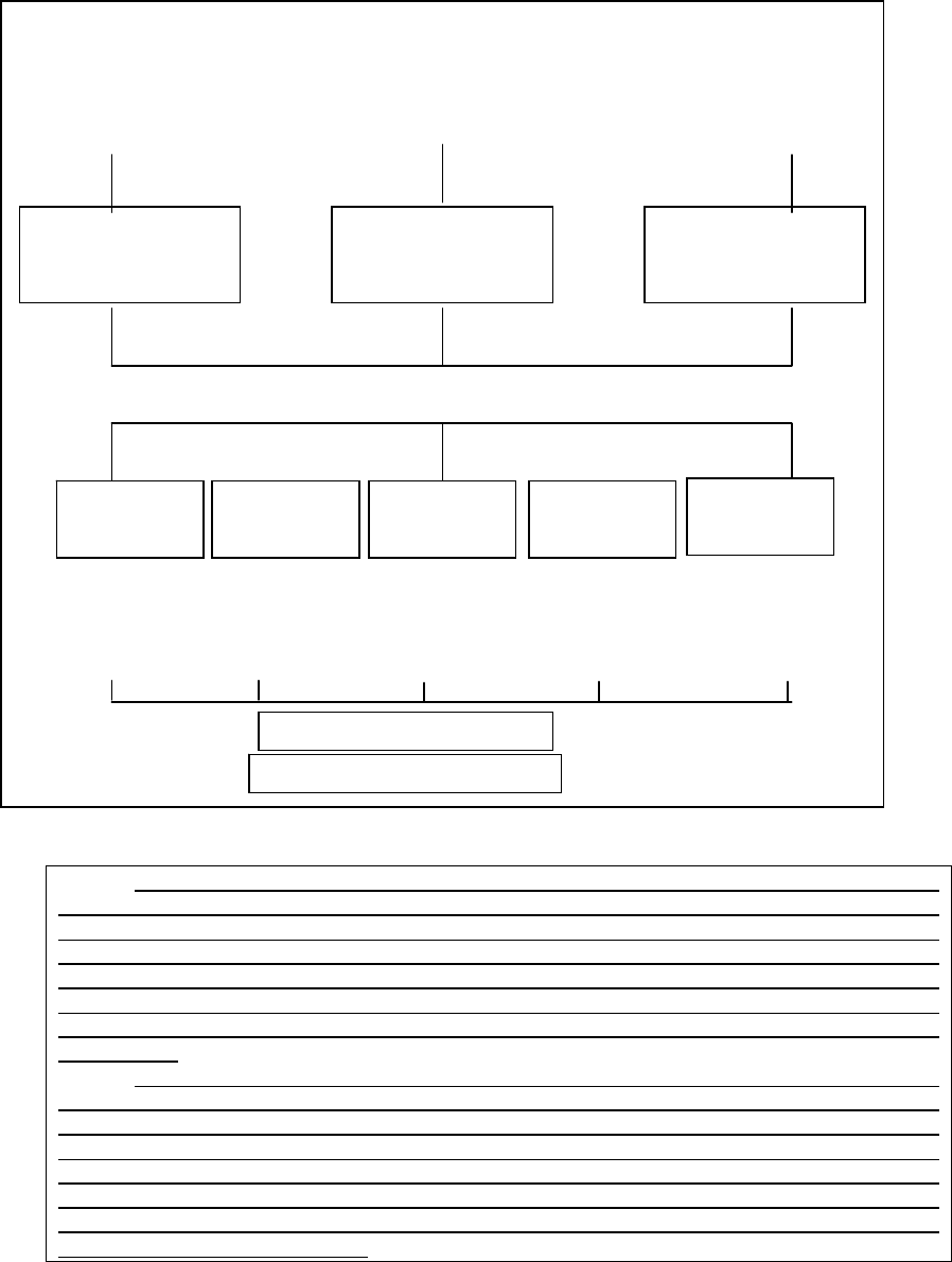
250
Graphics: 9.1
The sectional incharge of every section regularly reports the progress of his section to his
superior. In this diagram, functional have deputy managers who control department sections.
The combined reports of different sections reach the department manger, called functional
manager. Different functional managers submit the progress of their departments to the
managing director. The brief summaries of departmental reports are submitted to the board of
directors for reviewing polices and making strategy for the future. An effective reporting system
will enable the top management to remain in constant touch with the progress of different
departments.
The sectional incharge of every section regularly reports the progress of his section to his
superior. In this graphics, Functional Managers have Deputy Managers who control
departmental sections. The combined reports of different sections reach the departmental
manager, called functional manager. Different functional managers submit the progress of their
departments to the Managing Directior. The brief summaries of departmental reports are
submitted to the Board of Directors for reviewing policies and making strategy for the future. An
effective reporting system will enable the top management to remain in constant touch with
progress of different departments.
9.11 PRINCIPLES OF A GOOD REPORTING SYSTEM
Reporting to Management
Sectional Incharge
Department - B
Sectional Incharge
Department - A
Sectional Incharge
Department - C
Deputy Manager
Department - A Deputy Manager
Department - A Deputy Manager
Department - A
Controller Purchase
Manager
Factory
Manager Sales Personne
Functional Area
Maintenance
of Account Incharge of
Production Incharge of
Purchase Incharge of
Marketing Incharge
of
MANAGER
BOARD OF DIRECTORS
251
A good reporting system is helpful to the management in planning and controlling.
Every level of management needs information relating to its activities so that effective
planning may be undertaken and current activities may be controlled and necessary
corrective measures may also be taken in time, if needed. Some general principles are
followed for making the reporting system effective. These principles are discussed as
follows:
1. Proper flow of information: A good reporting system should have a proper
flow of information. The information should flow from the proper place to the
right levels of management. The information should be sent in the right form
and at a proper time so that it helps in planning and co-ordination. The
frequency of reports will depend upon the nature of report, the types of data
required for preparing the information and cost involved in preparing such
reports. The flow of reports should be such that it does not cause delay in
taking decisions. The reports should flow at regular intervals so that
information needs of different managerial levels are met at a proper time.
Flow of information is a continuous activity and affects all levels of the
organisation. Information may flow upward, downwards or sideways within
and organisation. Orders, instructions, plans etc may flow from top to bottom.
Reports grievances, suggestions etc. may flow from button to top,
Notifications, letters; settlements, complaints may flow from outside.
Information also flows sideways from one manger to another at the same level
through meetings discussions etc.
2. Proper timing: Since reports are used a controlling device so they should be
presented at the earliest or immediately after the happenings of an event. The
time required for preparation of reports should be reduced to the minimum; for
252
routine reports the period should be known and strictly adhered to. It will be a
waste of time and effort to prepare information, which is too late to be of any
use. The absence of information when needed will either mean wrong
decisions or deferment of decisions on matters, which may be urgent in nature.
3. Accurate information: The information should be as accurate as possible. If
the information supplied is inaccurate it may result in making wrong
decisions. However, the degree of accuracy may differ in different reports.
Sometimes, fractional information may be supplied as a guide for future policy
making, so the degree of accuracy may be less. The supply of exact figures
may involve a problem of understanding. Approximate figures are more
understandable than accurate figures given upto paise. Accuracy should also
not involve excessive cost of preparation nor should it be achieved at the
sacrifice of promptness of presentation. It will be better to have approximate
figure at a proper time than delayed information prepared accurately.
4. Basis of comparison: The information supplied through reports will be more
useful when it is supplied in comparison with past figures, standards set or
objectives lay down. The comparison of information with past or budgeted
figures enables the reader to find out trends of variations. The decision taking
authority will be able to make use of comparative figures while taking a
decision. Corrective measures can also be initiated to improve upon the past
performance. The management accountant can make the reports more useful
by giving his own interpretations to the information.
5. Reports should be clear and simple: The purpose of preparing reports is to
help management in planning, co-ordinating and controlling. This purpose can
be achieved only when the readers easily understand the reports. The
253
information should be presented in a clear manner by avoiding extraneous
data. Only relevant important information should become the part of a report.
If supporting information cannot be avoided then it should either be given in
appendix or separate chart should be attached for it. The method of presenting
information should be such that it attracts the eye, and enables the reader to
from an opinion abut the information. The graphic presentation of information
will enable the reader to find out the trends and also to determine deviations
more quickly than in other methods. The arrangement of presentation should
be brief, clear and complete. Simplicity is a good guide for reports
preparation.
6. Cost: The benefit derived from reporting system must be commensurate with
the cost involved in it. Though, it is not possible to assess the benefit of this
system in monetary terms, there should be an endeavour to make the system as
economical as possible.
7. Evaluation of Responsibility: The reporting system should enable the
evaluation of managerial responsibility. The targets are fixed for various
functional departmental heads. The record of actual performance is monitored
along with the standards so as to enable management to assess the
performance of different individuals. So, management reporting should be
devised in a way that it helps in evaluating the work assigned to various
persons.
9.12 PROCESS OF REPORT WRITING
The process of designing and writing a report consists of three stages. These stages
are as follows:
9.12.1 DECIDING THE NATURE AND PURPOSE OF THE REPORT

254
The first stage is to know the type of the report. Whether the report is statutory or
non-statutory. Its type shall determine the nature and shape of the report. It is also
very essential to know the purpose or object of the report. The purpose shall
determine the other two stages.
9.12.2 PLANNING STRUCTURE OF THE REPORT
There is no one-way to design the structure of the report. But following parts are
common in any report.
(i) Heading: A short. Clear, meaningful and attractive heading or title is
necessary for a report. Title or heading should indicate the subject matter of
the report.
(ii) Address: Every report is written for some one. So it is essential to write the
name of reader or readers. Report must be addressed to some person or body
of persons.
(iii) Contents: It is a list of chapters of the report. The contents of the report are
listed in serial order along with page numbers on which such contents are to be
found. Contents should be arranged logically.
(iv) Terms of reference or introduction: It gives the reasons for writing a report.
Brief description of the problem is stated. The object and scope of
investigation are also given in this part.
(v) Body of the report: This part is most important and lengthy. The writer
presents here the facts and data collected by him. Use of tables, graphs, and
diagrams can be made here or in appendices. The analysis of data is shown in
this part.
(vi) Recommendations: This part is the summary of the report and consists of
conclusions and recommendations. The conclusions are made on the basis of
STRUCTURE OF THE REPORT
(i) Heading
(
ii
)
Address
255
the facts and collected data. Recommendations or suggestions are given on the
basis of conclusions.
(vii) Reference and appendices: It is customary to mention, list of references and
bibliography indicating the sources from where the writer has taken material
for writing the report. Appendices contain diagrams, statistical tables,
specimen forms etc.
(viii) Signature. The person responsible for its preparation should sign every report.
The chairman should sign any report submitted by a committee. It is advisable
to mention date on the report.
9.12.3 DRAFTING OF REPORT
Drafting of a report is an important stage in report writing. This stage includes
following considerations.
(i) Collection of data and its analysis. First step in drafting is collecting
information, facts and data necessary for the purpose of the report. Data can be
collected from secondary or primary sources. Data is collected by
investigations, observations, and interviews or by survey etc. Collected data
has to be classified tabulated, edited and analysed. The collected data has to be
arranged logically and conclusions are drawn.

256
(ii) Format of a report. The format of a repot, which has already been explained.
It is concerned with the layout of the report and arrangement of the data. It can
be standardised for the purpose. Following is a specimen of a report form. If
report is in a letter form then it has salutation and a complimentary close. If
report is in memorandum form, both salutation and complimentary close may
be dispensed with.
Address (s) Date
Dear Sir (s)
Title
1. Terms of Reference
2. Finding of Investigation.
3. Conclusions
4. Suggestions
Prepared by
(Signature)
(iii) Writing of report: Report writing is an art, which can be developed by
practicing report writing and by studying the reports of other writers. Reports
are written for other so the needs and style preferred by the reader should be
kept in mind while writing a report. The general principles of a good reporting
system, which have been explained earlier, will help in writing the report.
(iv) Presentation of report. General layout of a report should be pleasing to the
eye. Report may be typewritten, printed or handwritten depending on the
number of copies required. Sufficient space and margin should be kept on the
left hand side. Reports should be written on one side of the paper with double
spacing. Pages, paras and sections should be numbered. Use of diagrams,
illustrations, charts, and tables may be made and these should be numbered. If
report is voluminous or is liable to constant handling it should be in bound
form.
9.13 SUMMARY
257
To know the present situation of the business and to formulate the policies for future
in business, reports are very crucial item. The problems of control, co-ordination,
communication and decision-making may be handled properly with reports, which are
delivered by the subordinates to the superiors. The decisions have wider implication
for business as a wrong decision may lead to its closure. Management needs detailed
information before taking any decision. The good decisions can minimise cost and
have a long-term positive bearing on the results. In all, it is the management reporting
that furnishes useful quantum of knowledge in the form of reports.
9.14 SELF-TEST QUESTIONS
1. Explain MIS and Management Reporting.
2. What do you understand by report and its types? Why the reporting is
compulsory in the business world?
3. What are the basic principles of report writing?
4. Explain the various steps for installing the reporting system at the various
levels of management. Discuss them in detail.
5. What are the requisites for a good reporting system?
9.15 SUGGESTED READINGS
11. Ashish K. Bhattacharya, Principles and Practices of Cost Accounting (3rd.),
New Delhi: Prentice Hall of India Private Limited, 2004.
12. Charles T. Horngren, Cost Accounting, A Managerial Emphasis, Prentice Hall
Inc., 1973.
13. D. T. Decoster and E. L. Schafer, Management Accounting, New York: John
Willey and Sons, 1979.
14. John G. Blocker and Wettmer W. Keith, Cost Accounting, New Delhi: Tate
McGraw Publishing Co. Ltd., 1976.
15. R. K. Sharma and Shashi K. Gupta, Management Accounting-Principles and
Practice (7th.), New Delhi: Kalyani Publishers, 1996.

258
Subject: Management Accounting
Course: M. Com Author: Dr. Karam Pal
Course Code: MC-105 Vetter: Prof. M. S. Turan
Lesson: 10
ROLE OF COMPUTER IN ACCOUNTING
Objective: The foremost objective of this lesson is to generate some awareness
among the students with regard to the role of computer in accounting.
Lesson Structure
10.1 Introduction
10.2 The History of Computer
10.3 Old Methods and Machines Used in Accounting
10.4 Role of Computers in Accounting
10.5 Advantages and Limitations
10.6 Merging Accounting and Computer Applications
10.7 Self Assessment Exercise
10.8 Suggested Readings.
10.1 INTRODUCTION
The most common method of keeping the financial records of a company was
manual. A bookkeeper kept the journals, the accounts receivable, the accounts
payable and the ledgers in his best possible penmanship. In later years, an
accounting machine, which was capable of performing normal bookkeeping
functions, such as tabulating in vertical columns, performing arithmetic
259
functions, and typing horizontal rows was used. The billing machine, which
was designed to typewrite names, addresses, and descriptions, to multiply and
extend, to compute discounts, and to add net total, posting the requisite data to
the proper accounts, and so to prepare a customer’s bill automatically once the
operator has entered the necessary information, was used. Early accounting
machines were marvels of mechanical complexity, often combining a
typewriter and various kinds of calculator elements. The refinements in speed
and capacity made possible by advances in electronics and operating
complexity of these machines. Many of the newer “generations” of accounting
machines are operated by a computer to which they are permanently connected.
Computers are rapidly changing the nature of the work for most accountants
and auditors. With the aid of special software packages, accountants summarize
transactions in standard formats for financial records and organize data in
special formats for financial analysis. These accounting packages greatly
reduce the amount of tedious manual work associated with data management
and recordkeeping. Computers enable accountants and auditors to be more
mobile and to use their clients’ computer systems to extract information from
databases and the Internet. As a result, a growing number of accountants and
auditors with extensive computer skills specialize in correcting problems with
software or in developing software to meet unique data management and
analytical needs. Accountants also are beginning to perform more technical
duties, such as implementing, controlling, and auditing systems and networks,
and developing technology plans and budgets.
Increasingly, accountants also are assuming the role of a personal financial
advisor. They not only provide clients with accounting and tax help, but also
help them develop personal budgets, manage assets and investments, plan for
retirement, and recognize and reduce exposure to risks. This role is a response
to client demands for a single trustworthy individual or firm to meet all of their
financial needs. However, accountants are restricted from providing these
services to clients whose financial statements they also prepare.
260
Persons planning a career in accounting should have an aptitude for
mathematics and be able to analyze, compare, and interpret facts and figures
quickly. They must be able to clearly communicate the results of their work to
clients and managers. Accountants and auditors must be good at working with
people, as well as with business systems and computers. At a minimum,
accountants should be familiar with basic accounting software packages.
Because financial decisions are made based on their statements and services,
accountants and auditors should have high standards of integrity.
Increased awareness of financial crimes such as embezzlement, bribery, and
securities fraud will also increase the demand for forensic accountants to detect
illegal financial activity by individuals, companies, and organized crime rings.
Computer technology has made these crimes easier to commit, and it is on the
rise. But, development of new computer software and electronic surveillance
technology has also made tracking down financial criminals easier, thus
increasing the ease and likelihood that forensic accountants will discover their
crimes. As success rates of investigations grow, demand will also grow for
forensic accountants.
Proficiency in accounting and auditing computer software, or expertise in
specialized areas such as international business, specific industries, or current
legislation, may be helpful in landing certain accounting and auditing jobs. In
addition, employers increasingly seek applicants with strong interpersonal and
communication skills. Because many accountants work on teams with others
from different backgrounds, they must be able to communicate accounting and
financial information clearly and concisely. Regardless of one’s qualifications,
however, competition will remain keen for the most prestigious jobs in major
accounting and business firms.
10.2 THE HISTORY OF COMPUTER
The logical first step in becoming computer literate is to appreciate the origins
of computers. Computers are the result of a long history of mathematical
261
exploration and innovations. They have their earliest roots in primitive systems
of counting that relied on fingers and toes or stones to enumerate objects.
Historically, the most important early computing instrument is the abacus,
which has been known and widely used for more than 2,000 years. It is simply
a wooden rack holding parallel wires on which beads are strung. When these
beads are manipulated (moved along the wire) according to “programming”
rules that the user must memorize, all ordinary arithmetic operations can be
performed. Another computing instrument, the astrolabe, was also in use about
2,000 years ago for navigation.
Blaise Pascal is widely credited with building the first “digital calculating
machine” in 1642. It performed only the addition of numbers entered by means
of dials and was intended to help Pascal’s father, who was a tax collector. In
1671, Gottfried Wilhelm von Leibniz invented a computer that was built in
1694. It could add, and by successive adding and shifting, multiply. Leibniz
invented a special “stepped gear” mechanism for introducing the addend digits,
and this mechanism is still used. The machine of Leibniz was in a sense a
forerunner of the mechanical desk calculator invented by Charles X. de Comar
in 1820.
The first real computer didn’t change the world. It was never built. It existed, in
fantastic detail, in the mind of a grumpy English mathematics teacher named
Charles Babbage around the time of our civil war. He loved problems and
puzzles, as do computer people today. He taught himself arithmetic, and when
he went to college, he knew more algebra than his teacher. He invented
speedometers and a machine for playing tic-tac-toe. Later he built an adding
machine that could solve a particular kind of problem. Then, he began to
design an “analytical engine” that could solve any kind of arithmetic problem.
Babbage put together the idea of instructions sorted in punched cards with the
idea of a calculating machine. To set up the machine to solve a new problem—
weave a new arithmetic pattern—he would just change cards. The two ideas
added up to a sum vastly greater than its parts. Inside Babbage’s head was the
262
first true computer. His design was practical, but it required cogwheels and
gears and other parts that the machinists of his time could not make, and so the
analytical engine had to wait a hundred years to be translated from a brilliant
idea to working machine. The next influential invention was the census
machine of Herman Hollerith. In the late nineteenth century, census taking had
become a major task; tabulation of such a vast amount of data was slow and
problematical. In an effort to find a faster way to compile raw statistical data,
the Census Bureau sponsored a contest. Herman Hollerith’s device was chosen
the most effective and practical.
Hollerith had designed a device that read data from punched cards and kept
track of the count. The keypunch system of data processing was popular for
many years, although recently it has succumbed to faster and less cumbersome
methods. Hollerith was so successful that he left the census Bureau in 1896 to
form the International Business Machine Corporation -IBM, a recognized
leader in the field of data-processing technology even today.
This concept led to systems using electromechanical devices, in which electric
power provided mechanical motion—such as for turning the wheels of an
adding machine. Such systems soon included features to feed in automatically a
specified number of cards from a “read-in” station; and feed out cards punched
with results. By modern standards the punch-card was slow, typically
processing from 50 to 250 cards per minute, with each card holding up to 80
decimal numbers. At the time, however, punched cards were an enormous step
forward.
Vannevar Bush, a professor at MIT, built and demonstrated a differential
analyzer in 1930. It was large, and had many gears, but it used electric motors.
It worked, and could be programmed to perform many different types of
calculating work. Bush’s machine was also the first to use titles. His machine
could store numbers or quantities of electricity in one part of the system. This
ability led some to name Bush the Father of the Electronic Computer. The day
263
of the gear driven computer was almost over. Konrad Zuse, a German engineer,
and Howard Aiken, a Harvard math professor, both built hybrid (part
mechanical, part electronic) machines in the period between 1930 and 1950.
Both used binary arithmetic and both used electric relays to perform math
operations.
Professor Aiken worked in conjunction with IBM and had discovered
Babbage’s work. The ideas were so close to Aiken’s that he thought he had
received a personal message from the past. Professor Aiken was building a
computer named Mark I. Instead of punched cards, Professor Aiken used rolls
of punched paper to tell the machine what to do. Electricity turned the counter
wheels, and eight hundred thousand switches, buttons, and other electrical parts
filled a room three times as big as an ordinary living room.
In 1942, two men and their associates were at work at the Moore School of the
University of Pennsylvania on a machine which, while embodying enormous
advances in automatic computing, was less famed than the Mark I. It was not
operational until two months after the Japanese surrender and therefore did not
get credit for helping to win World War II. The co-inventors of ENIAC
(Electronic Numerical Integrator and Calculator) which was actually the
world’s first electric computer were Dr. J. Prosper Eckert, an electrical
engineer, and Dr. John Mauchly, a physicist. It would have been easily possible
for them to build ENIAC twelve to fifteen years earlier, as it would have been
possible to build the Mark I—all of the components and the theory required
were in existence except for the fact that nobody put up the money or had the
incentive to do so. The patron of ENIAC was the United States government,
more specifically, the Army.
The most significant feature of ENIAC was that it introduced vacuum tube
technology, and no longer were calculations and operations performed by
moving mechanical parts. This feature allowed for greatly increased speed of
performance. The next computer was developed by Mauchly, Eckert, and
264
others and was called the Electronic Discrete Variable Automatic Computer
(EDVAC). It was smaller and more powerful than its predecessors. It also had
two other important features: it used binary numbering systems, and it could
internally sort instructions in numerical form. Today, a1l data and programs are
stored in binary form. This method of storing instructions inside the computer
is far more efficient than paper tape storage used in earlier devices.
Another member of the first generation of computers was the Electronic
Delayed Storage Automatic Computer (EDSAC) built at Cambridge University
in England. This computer introduced the concept of stored programs. Before
this, computers often had to be rewired to be used for various operations. Their
memories were incapable of storing more than one program at a time. EDSAC
helped eliminate time consuming and costly rewiring procedures.
In 1946, Mauchly and Eckert formed a corporation to build computers for
commercial use; the UNIVAC (1951) was the first electronic computer used by
large business firms. This launched the major growth of computers into the
business field. The first generation of computers, which thrived from 1951
until 1964, was characterized by vacuum tube technology. Although they were
amazing devices in their time, they were large, took up valuable space, were
expensive to operate, and required almost constant maintenance to function
properly. The next generation of computers attempted to resolve some of these
problems.
The second generation of computers extended from 1959 until 1964 and was
characterized by transistor technology. The transistor was developed by John
Bardeen and others at the Bell Laboratories in New Jersey. Bardeen studied
substances that permitted a limited amount of electricity through them—
semiconductors. Transistors using semiconductor material could perform the
work of vacuum tubes and took up less space.
265
Because transistors were smaller, the distance between operating parts was
reduced and speed of performance was increased significantly. Transistors
were also much cooler than vacuum tubes, reducing the need for expensive air
conditioning in areas where computers were housed. Transistors did present
several problems, though. They were relatively expensive because each
transistor and its related parts had to be individually inserted into holes in a
plastic board. Also, wires had to be fastened by floating boards in a pool of
molten solder. Even thought the distance between individual parts was reduced,
it was still great enough to limit speed of computer operations. The next
generation of computers helped to alleviate some of these problems.
The development of integrated circuits in 1963 spawned the third generation of
computers, lasting from 1964 to 1975. Integrated circuits developed from a
need to mass produce transistors in a few simple production steps. The
production process begins when tubes of silicon are sliced into wafer thin disks
that are chemically pure and cannot hold electrical charge. Then a preconceived
design is etched onto the surface of the wafer with the use of light rays.
The integrated circuit continued the trend toward miniaturization that has
resulted in the popularity of the microcomputer and the personal computer
system. Integrated circuit technology spawned a generation of computers that
had greater storage capacity and technically increased speeds of performance.
Many accessory devices were developed and marketed, such as magnetic tape
drives and disc drives. Popular programming languages were developed and
refined, many of which are still in use today.
Third generation computers are not aimed at specific applications such as
business or scientific use. Rather, they were designed as general purpose
computers. They represented a giant leap forward in the data processing field.
Not only were speed and reliability enhanced, but power consumption was
decreased markedly. Computers became smaller and less expensive, putting
266
computer power into the hands of a greater number of users than ever before.
Computer Technology began to snowball.
Engineers were not satisfied with the degree of miniaturization that resulted
from the integrated circuit. Also, the integrated circuits of the third generation
were designed primarily with chips having the only function. As engineers
learned how to manufacture chips more easily, they conceived the idea of
grouping an assortment of functions on a single chip, creating a microelectronic
“system” capable of performing various tasks required for a single job. This
technology became known as Large Scale Integration (LSI). Thus, the fourth
generation of computers was born in the mid-1970.
LSI technology has also been responsible for the recent popularity of the
microcomputer. These “Litt1e giants” fit easily on a desk top and put computer
power in the hands of an increased number of people. Declining prices of
powerful computer systems have also encouraged development of the
electronics field in genera1. LSI turned computer technology into big business,
and this trend will certainly continue in the foreseeable future.
A hint of tomorrow’s computer capability can be found in the IBM 3081,
introduced in 1980. This computer is twice as powerful as its immediate
predecessor. It was designed with Very Large Scale Integrated (VLSI) circuitry
further increases the speed at which computers are able to function.
Multiprocessing—the simultaneous running of several programs by one
computer is likely to develop further in the fifth generation of computers.
Computers will continue to get smaller as well as prices becoming lower.
10.3 OLD METHODS AND MACHINES USED IN ACCOUNTING
The most common method of keeping the financial records of a company was
manually. A bookkeeper kept the journals, the accounts receivable, the
accounts payable and the ledgers in his best possible penmanship. In later
267
years, an accounting machine, which was capable of performing normal
bookkeeping functions, such as tabulating in vertical columns, performing
arithmetic functions, and typing horizontal rows was used. The billing
machine, which was designed to typewrite names, addresses, and descriptions,
to multiply and extend, to compute discounts, and to add net total, posting the
requisite data to the proper accounts, and so to prepare a customer’s bill
automatically once the operator has entered the necessary information, was
used. Early accounting machines were marvels of mechanical complexity,
often combining a typewriter and various kinds of calculator elements. The
refinements in speed and capacity made possible by advances in electronics
and operating complexity of these machines. Many of the newer “generations”
of accounting machines are operated by a computer to which they are
permanently connected.
10.4 ROLE OF COMPUTER IN ACCOUNTING
Because of the minute by minute change in finances, accurate record keeping is
critical. Computerizing a business’s general ledger, payroll, and other
accounting tasks increases office efficiency. With a computer, you can request
and receive an in house balance sheet, an income statement, or other
accounting reports at a moment’s notice. While keeping your checkbook on a
computer may not be practical, computers are great for handling complex home
financial records. You can get statements on net worth and year’s tax
deductible expenses within minutes.
A. Spreadsheets
Electronic spreadsheets allow you to do anything that you would normally do
with a calculator, pencil and columnar scratch pad. Spreadsheets were
primarily designed for managers who in the process of planning must do “what
if” calculations. Due to their flexibility, electronic spreadsheets have found
their way into small businesses and, to a lesser extent to homes. A typical
integrated double entry accounting system will contain some or all of the
268
following components: accounts receivable, accounts payable, general ledger,
inventory, order entry, payroll, time, and billing.
It takes its name from the accountant’s spreadsheet—a sheet of paper with rules
for rows and columns—on which such work was usually done. Spreadsheet
programs are much faster, more accurate, and easier to use than traditional
accounting techniques. The programs are widely used on personal computers
for keeping sales, expense and inventory records, and for budgeting and
forecasting future sales and expenses. As a result of these and many other
applications, computer spreadsheets have become the most important of all
software tools for modern businesses.
Early programs such as VisiCalc provided 254 rows and 63 columns for
entering data and formulas for calculations. Some modern programs for
computers with large memories provide thousands of rows and hundreds of
columns. VisiCalc was introduced by Robert Frankston, a young computer
programmer, and Dan Bricklin, a Harvard Business School student who was
looking for a way to use the power of a computer to simplify complex time-
consuming financial analyses. VisiCalc proved so useful in such applications
that it provided an entry for personal computers into the business world. In
1980, the Sorcim Corporation introduced SuperCalc, a similar spreadsheet
program for personal computers using the CPM operating system.
A new generation of computer software for business began with integrated
spreadsheet programs, which can be used to prepare spreadsheets, create
graphs, and manage data. In such programs, for example, it is easy to display
spreadsheet data in the form of a graph or to transfer data from a data base to a
spreadsheet. One of the first such programs was Lotus 1-2-3, an immediate
success following its introduction in 1983.
In the third generation of integrated business software, spreadsheet, graphics,
and data management capabilities were supplemented by word processing and
269
communications capabilities. With such comprehensive programs, it became
possible to create multiple windows on the computer display. Each window
could contain a different application—a graph in one, a spreadsheet in another,
and word processing in a third. The window capabilities of integrated programs
such as Symphony and Framework make it easy, for example, to transfer a
spreadsheet or a data-base report to word processing for styling and formatting
before printing.
B. General Ledger
General Ledger is a labor saving device for the preparation of financial
statements and for establishing multiple income and cost entries.
C. Accounts Receivables
Accounts receivable, when computerized, can get your bills out the same day
you’ve performed a service. An accounts receivable module prepares invoices
and customer accounts, adds credit charges where appropriate, handles
incoming payments, flags your attention to customers that are delinquent, and
produces dunning notices. It allows you to have daily cash control. You get out
the bills on time, yet you avoid errors such as billing a customer twice for the
same item. The further advantage is that debits and credits are posted
automatically to the general ledger, order entry, and in some instances
inventory, once they are entered in accounts receivable.
D. Accounts Payables
Accounts payable, when computerized, will provide for purchase order control,
invoice processing, payment selection and handling, check writing and control,
cash-requirements, forecasting, and format preparation. It will also double-
check the accuracy of the vendor’s invoice, and some software systems will
cross-check it against the purchase order and the inventory module.
E. Inventory Control
Inventory Control module has multiple functions, including tracking inventory
for both costing and tax purposes, controlling purchasing (and the overall level
270
of expenditure) and minimizing the investment in inventory (and subsequent
loss of cash flow). The payroll module prepares and prints payroll checks,
including all itemized deductions. It is integrated with the general ledger so you
automatically set aside the correct amount for FICA and withholding.
F. Point of Sale
Point of sale module captures all sales information at (or in place of) the cash
register, including salesperson, date, customer, credit information, items, and
quantity sold. It can produce sales slips or sales invoices, plus it reports on
items, customer, and salesperson activity.
G. Purchasing and Receiving
Purchasing and receiving module can represent an invaluable addition. It can
generate purchase orders and track their fulfillment. You can find out which
vendors are delivering on time and saving you the expense of having to follow
up on partial and incomplete orders.
H. Time and Billing Module
Time and billing module reduces manual and clerical work, simplifies the
billing process, prompts you and your partners to bill on time, reduces unbilled
work-in progress, minimizes unreported time, reduces unbilled time, measures
and analyzes non-chargeable time and provides criteria to analyze staff
performance. Because a computerized accounting system is basically a
computerized data management system, the disposition of labor is almost the
same. One staff member must serve as a data-base manager and be in charge of
setting up the chart of accounts, establishing the interrelationships among the
files and establishing and maintaining an audit trail.
10.5 ADVANTAGES AND LIMITATIONS OF COMPUTER USE
The most important advantage of using the computer is the speed with which
we can get accounting done. In addition, we find that it is very easy to do
accounting functions. Posting to the ledger, a tedious task of double entry,
when done directly from the general ledger module, can be largely automated
271
when done through special purpose modules like accounts payable or accounts
receivable. With an accounts receivable module, you just need to enter the
actual cash totals of items purchased and the software distributes these amounts
to the general ledger so they become credits to corresponding revenue
accounts. At the same time, an offsetting entry is made automatically to the
accounts receivable account.
With a computer, one can receive a balance sheet, income statement or other
accounting reports at a moment’s notice. We also find that some day to day
data entry can be turned over to relatively unskilled workers.
When you use a computer, it is possible that data can be lost because of
hardware or software damage. Since the computer has no judgement of its own,
it does not pick up on errors as a human being does. There can be loss of data
due to accidents like fire etc... There can be loss of data or change of data due
to fraud or embezzlement. There can be loss or unavailability of data due to
loss of staff. Inaccurate data may be due to clerical error or mistakes in
programming. Total security is economically unachievable and some failures
must be expected. The right level of expenditure on security measures will
minimize the sum of the cost of the measures and the expected loss. There will
always be some risks that are best shared through insurance, rather than
prevented or avoided.
Much computer-related crime is opportunist: People who were not seeking
any advantage had temptation thrust under their noses. Copies of computer
printouts get mis-directed, or thrown in a waste paper basket in a public place.
Magnetic tapes from bankrupt companies have been sold with data still on
them. Often a programming error reveals a system flaw: someone who by
chance reads a magnetic tape file that he should have been writing discovers
interesting data on it.
272
Sabotage, vandalism, malicious damage, and arson tend to be even more
destructive than the Acts of God they emulate. Political and industrial action,
riots and civil commotions, may not be aimed specifically at the computer but
they can be very effective in preventing its operation.
Fraud and embezzlement are usually achieved on a computer system by
altering data or programs. There are numerous techniques, varying from
additions and deletions to input data, through changing the standing
information files, modifying the behavior of programs, to duplicating or
suppressing output. Although most frauds that have been reported had gone on
for some time, it could be that ‘one shot’ frauds have been more frequent but
more often escape detection.
Eavesdropping and stealing information by tapping telecommunications lines
requires the sort of technical skill which is very widely available (to the
surprise of those without technical education). It is possible to emulate a
legitimate user of a system, or discover his password through trickery or as the
result of carelessness, and thus have access to the information he would have,
such access can be very important for setting up more profitable operations,
such as taking money out of little used bank accounts, or concealing changes
made in files. There are other ways of trespassing, without using wire tapping.
For example, the magnetically encoded cards often used as keys to systems can
be copied and altered, giving the villain access to credit, cash or other valuable
assets.
Wherever a computer is used to handle an organization’s accounts, it can be
used as a means of attacking the funds it controls. In most computerized
bookkeeping systems, it is the computer which effectively causes credit
transfer; so by establishing false accounts, or diverting some of the contents of
the real ones, credit can reach a false beneficiary. The system can also be used
to conceal a change in the cost, or the illegitimate acquisition or the destruction
of tangible goods and services.

273
Duplication which is designed to minimize losses in the event of deliberate or
accidental threat can be used. Duplication is designed to ensure that the system
survives damage to any individual part. Duplication is also the fundamental
method of detecting errors in processing. Defense in depth is designed to make
the attacker overcome a series of barriers before he can damage any vital part
of the system. In addition, most companies have computer auditors who ensure
the integrity and accuracy of the organizations records, protect and conserve
the organization’s assets and prevent fraud, theft and error. These auditors also
ensure that systems will survive the hazards to which they are exposed.
10.6 MERGING ACCOUNTING AND COMPUTER APPLICATIONS
There has been increasing concern recently that accounting, the "language of
business," is not expressive enough to match the potential created by the
phenomenal growth of technology. While management accountants have taken
a lead role in developing frameworks for performance evaluation that
encompass financial and nonfinancial measures, the methods by which
antiquated accounting systems are designed prevent them from taking full
advantage of advances in information technology. If management accountants
were to get more involved in the process of software design, particularly
through models such as the resources, events, and agents (REA) model, they
could become more involved in supporting firm-wide strategic management
and control.
Management accountants have a greater opportunity to support corporate
strategy when they are involved in developing IT databases using a conceptual
design tool in concert with the balanced scorecard (BSC). We try to establish a
logical link between the design potential of the REA model and the
performance measurement framework of the BSC. This link provides the basis
for an integrated conceptual database design framework that will enable
management accountants to assist in the development of meaningful

274
accounting information systems and establish their role as partners in the
development and evaluation of corporate strategy and planning.
Peter Drucker spoke of the turbulence in accounting that is becoming evident
as the CFO's role in organizational strategy undergoes a transformation. Now
that structured tasks are computerized, which has resulted in reengineering and
some outsourcing of traditional accounting tasks, management accountants
who use only the traditional skills required for such tasks do so at their and the
profession's peril. The work of management accountants has become analytical
and decision oriented, but these financial professionals are unable to fully
realize the changes in their role unless they become partners in the design and
development of the information systems in their organizations. To become
partners, management accountants need to develop and identify tools that give
them greater insight into database development processes.
It is important to describe two developments in accounting: the resources,
events, and agents (REA) model and the balanced scorecard (BSC) model. The
two, operating together, can close the loop among the performance
measurement, strategic decision-making, and systems design functions of a
company.
The REA model, a conceptual model for database design, has the potential to
enable management accountants to play an intrinsic role in the design of
information systems. The balanced scorecard provides a framework for an
"integrated view" of the organization that extends beyond the traditional
financial view. It also provides a wealth of information about the firm that can
enable management accountants to define and describe entities in the database
more accurately.
Are there developments in accounting aimed to meet these challenges? The
traditional "accounting view" of the organization is insufficient to satisfy many
"information customers." Accounting systems, which are driven by

275
transaction-based financial accounting requirements, capture limited
characteristics of transactions. As a result, different functional areas maintain
parallel information systems to cater to their individual needs, causing
inefficiencies in data storage and making it difficult to integrate information
across functional areas.
The key problem is antiquated design and development of accounting systems.
The only planning in traditional accounting is the "chart of accounts," the first
step in the accounting cycle that focuses on financial transactions and
culminates in summarized, uniform financial statements. The accounting
system still depends largely on the debit-credit model that has a 700-year
history dating back to Lucas Pacioli. This model had validity in manual
systems and gave shape to accounting activities in traditional accounting. But
with changes in the nature and size of firms and the advent of databases and
online computing, this antiquated system has become a handicap to designing
information systems required for executive decision making.
This situation has largely left information systems development activities to
people in management information systems (MIS). MIS has developed the
sequence of activities called "systems development life cycle" (SDLC), which
includes systems planning, analysis, design, and implementation. Depicting the
information systems in terms of Michael Porter's value chain concepts helps us
gain insights into the issues that impact the development of corporate
information systems
The design phase of the SDLC adds value to the information system because it
helps determine the adequacy and relevance of information for decision
making. It is in this phase that the information for strategic and other decisions
is framed and determined. Currently, information systems personnel from MIS
departments, who are trained in technical aspects of information systems, play
the key role in systems design and implementation activities. Management
accountants, however, are in the position to be most knowledgeable about the

276
information value chain and the means through which it can add value.
Accordingly, as Michael Porter puts it, "No other business information system
has the ability to combine the performance of all functions of a business into
one set of measures, which has led accounting to be known as the 'language of
business.'" Peter Drucker, as quoted earlier, also predicted that the challenges
to information systems would not be technical but rather would be the ability to
translate data into information that is useful for decision making. Therefore, the
key benefit of the information value chain would be to collect and present
relevant information that would add value to control and decision-making
processes. But traditional accounting systems give only a limited view of the
organizational processes, which means management accountants are
handicapped from playing a major role in the overall systems design. What is
needed is an "integrated" and encompassing view of the organization. It can be
provided by the REA model and the balanced scorecard, with management
accountants deeply involved in both.
The REA model provides management accountants with a tool for designing
database systems. The balanced scorecard, a downstream activity in the
information value chain, provides a framework of performance measures that
can be used for communicating and measuring strategy and providing a
framework for systems design. The two tools converge in the design phase of
information systems development, and here management accountants have an
opportunity to create a new role for themselves in the information systems area.
Kaplan and Norton see "functional silos" as handicaps in the development and
implementation of strategy. They point out that, "Organizations are
traditionally designed around functional specialties such as finance,
manufacturing, marketing, sales, engineering, and purchasing. Each function
has its own body of knowledge, language, and culture. Functional silos arise
and become a major barrier to strategy implementation as most organizations
have great difficulty communicating and coordinating across these specialty

277
functions." Management accountants can play a key role in harnessing the
potential of a measurement system that encompasses the specialty functions.
Research has also helped in highlighting that systems design in the information
systems value chain can have an important impact on the effectiveness of
measurements. This confirms--and research supports--those management
accountants should be more involved in systems design and implementation. It
is at the design stage that these measures are fully integrated into the system.
The relationship between meanings attached to different measures and the data
that is collected must be consistent across functional areas and reflect business
activities. Research confirms that measures commonly used across business
units are more useful for decisions. This highlights the need for greater
uniformity and comparability of measures. In addition, the need to coordinate
and communicate strategy throughout the organization also confirms the need
for measures to cascade to different levels in the organization without changes
in meaning. For example, Kaplan and Norton have indicated a link between the
BSC implementation process and information systems when they point out that
"a newly formed team develops an implementation plan for the scorecard,
including linking the measures to databases and information systems,
communicating the balanced scorecard throughout the organization, and
encouraging and facilitating the development of second-level metrics for
decentralized units. As a result of this process, an entirely new executive
information system that links top-level business unit metrics down through
shop floor and site-specific operational measures could be developed"
(emphasis added). The design of information systems, therefore, is an
important component of implementing a BSC that conforms to corporate
strategy.
10.7 SELF ASSESSMENT EXERCISE
1. What do you think can be the major role of computer in accounting
particular in management accounting? Briefly explain any two roles
with examples.

278
2. The basic objective of computer applications in accounting is to make it
easily understandable to common users. Discuss a detailed and planned
reaction for the purpose
3. Assuming you are appointed the manager of a business organization
with an authority to put latest technology in place? Put up a detailed plan
for the purpose
4. Discuss and illustrate with suitable examples the effective role of
computer in accounting required in modern times.
10.8 SUGGESTED READINGS
1. Kenton B. Walker and Eric L. Denna, "A New Accounting System Is
Emerging," Management Accounting, July 1997, pp. 22-30.
2. Michael Porter, Competitive Advantage: Creating and Sustaining Superior
Performance, Simon & Schuster, New York, N.Y., 1985.
3. Robert S. Kaplan and David P. Norton, "Using the Balanced Scorecard as a
Strategic Management System," Harvard Business Review,
January/February 1996, pp. 75-85.
4. Mary A. Malina and Frank H. Selto, "Communicating and Controlling
Strategy: An Empirical Study of the Effectiveness of the Balanced
Scorecard," Journal of Management Accounting Research, 2001 (Volume
13), pp. 47-90.
5. Robert S. Kaplan and David P. Norton, "The Balanced Scorecard--
Measures That Drive Performance," Harvard Business Review,
January/February 1992, pp. 71-79.
6. Christopher Ittner and David F. Larcker, "Are Nonfinancial Measures
Leading Indicators of Financial Performance?: An Analysis of Customer
Satisfaction," Journal of Accounting Research, 1998 (Volume 36), pp. 1-35.
7. Rajiv D. Banker, G. Potter, and Dhinu Srinivasan, "An Empirical
Investigation of an Incentive Plan that Includes Nonfinancial Performance
Measures," The Accounting Review, January 2000, pp. 65-92.
8. Venky Nagar and Madhav V. Rajan, "The Revenue Implications of
Financial and Operational Measures of Product Quality," The Accounting
Review, October 2001, pp. 495-513.

279
Course : Management Accounting Writer : Dr. M.C. Garg
Course Code : MC-105 Vetter : Dr. B.S. Bodla
LESSON-11
INFLATION ACCOUNTING
Objective: On completion of this lesson, you should be able to (a) Explain the
impact of increase in price level on financial statements (b) to make
adjustments in (conventional) financial statements for increase in
general price level resulting in decrease in purchasing power of money
and (c) to prepare financial statements on the basis of current cost
instead of historical cost.
LESSON STRUCTURE
11.1 Introduction
11.2 Reasons for Inflation Accounting
11.3 Limitations of Historical Accounting
11.4 Methods of Inflation Accounting
11.5 Advantages of Inflation Accounting
11.6 Disadvantages of Inflation Accounting
11.7 Summary
11.8 Self Assessment Questions
11.9 Suggested Readings
11.1 introduction to inflation accounting
Inflation is a state to inflation accounting in which purchasing power of money goes
down or conversely there is more money in circulation than is justified by goods and
services. The effect of inflation is that prices of assets go up and the accounts
prepared on the basis of conventional accounting system present much distorted
figures to the users of accounts.
Accountants prepare Profit and Loss Account and Balance sheet at historical costs.
Profit is the difference between revenue and costs. Revenue reflects the current value
whereas costs represent current as well as historical costs. Thus the profit is overstated
measured in terms of money and the value of money is fluctuating due to inflation,
any measurement with fluctuating scale is unreliable and would distort the true
financial position of the organization.
In such cases to make the measurement perfect, the scale should be kept steady. If this
is not possible, an alternative should be evolved to adjust the effects of fluctuating
changes in money value and make the financial statements reflect current values in
real terms. Management Accountant has responsibility towards shareholders and
internal management of the organisation to appraise the true financial position of the
organisation.
Inflation Accounting devised to show the effect of changing cost and prices on affairs
of a company during the course of relative accounting periods. It is also known as
‘Accounting for price level changes’.
11.2 Reasons for Inflation Accounting
Financial accounts are the basis on which the success of the business is measured and
on which investors can find out whether or not their investment is safe and will
produce a reasonable return for them. Financial accounts, therefore, have a significant
effect on the business, and shareholders are particularly interested in them from the
280
point of view of not only obtaining a good return on their investment but also of
maintaining the value of that investment.
But if this value is expressed in terms of historical costs, without allowing for the
inspect of inflation, it could be illusory. Hence, the need for inflation accounting. The
purpose of inflation adjusted accounting is to restore the principle of matching current
revenues with current costs or current purchasing power to the Profit and Loss
Account, thus removing the inflationary element from historic cost profit and/or
allowing the concept of physical capital maintenance to be adopted.
Inflation accounting is a system of accounting which regularly records all items in
financial statements at their current values. The system recognizes the fact that the
purchasing power of money is decreasing day-by-day during inflation and finds out
profit or loss or states the financial position of the business on the basis of the current
prices prevailing in the economy.
11.3 Limitations of Historical Accounting
Now there is a near unanimity among the accountants that historical cost accounts
suffer from many serious limitations during the period of rapidly changing prices. The
following are the main limitations of historical accounts :
1. Utility of accounting records seriously impaired : Financial statements or
reports based on historical cost fail to reflect the effect of such changes in
purchasing power on the financial position and profitability of the firm.
Financial statements may be incorrectly interpreted unless adjustments are
made to place the data on the current price level. In this way, the utility of the
accounting records not taking care of price level changes is seriously impaired
and makes a demand on the accounts for adjusting financial accounting for
inflation to know the real financial position and profitability of a concern.
2. Unrealistic profits : Under the historical accounting system, depreciation
calculated on the basis of historical cost of old assets is usually lower than that
of those calculated at current value or replacement value. This results in more
profits on paper which, if distributed in full, will lead to various consequence
of over statement of profits as more taxes, more bonus to the employees, more
dividend to shareholders etc. Thus there will be reduction of capital and
ultimately the company may go into liquidation.
3. Insufficient provision of depreciation : Under the historical accounting
system, depreciation is calculated on the original cost of fixed assets with the
result that only an amount equivalent to the original cost of the fixed assets is
available for its replacement when its life is over. But the replacement cost of
the asset will be more than the original cost on account of inflation so that the
replacement provision made by way of depreciation charge on the original
cost will be insufficient for the purpose.
According to the Economic Survey, “there is now considerable evidence that
the steep increase in cost of machinery and equipment in recent years is
affecting not only new investment but also modernization and replacement of
existing equipment. In a period of rapidly rising prices depreciation formulae
based on historical cost cease to provide adequate resources for the
replacement of the existing worn out equipment. Moreover, in industries under
price control, so long as the calculations of permissible rates of return continue
to be based on historic cost of fixed capital in use, there is a built in
disincentive to new investment.” Most of the industrial sickness in India is due
to the insufficient funds available for replacement and renovation on account
of charging depreciation on historical cost.

281
4. Fixed assets values are unrealistic : In times of rising prices, the
conventional system of accounts based on historical cost does not give a true
and fair view of the business enterprise as is required under the Companies
Act, 1956 as fixed assets are shown at their historical cost and not at current
values.
5. Different basis : In conventional system of accounting, fixed assets are
shown at the historical costs whereas operating expenses and incomes are
taken at current prices. Thus different bases adopted are not desirable for
having correct and reliable information about the business.
6. Return on capital employed misleading : Under historical cost accounting
system the profits are overstated and fixed assets are understated specially
when there is increase in the price of the old fixed assets. Return on capital
employed which is very useful for the valuation of the business by its owners,
creditors and management will not be correct and may lead to misleading
decisions. This will be clearer from the following example.
Rs.
Fixed Assets at cost 20,00,000
Less : Accumulated Depreciation
12,00,000
---------------
8,00,000
Add : Current Assets 10,00,000
---------------
Total Assets 18,00,000
Less : Current Liabilities 4,00,000
---------------
Capital Employed 14,00,000
Net profit after tax @ 50% and 10% depreciation on original cost is Rs. 2,80,000.
Replacement cost of the fixed assets is Rs. 40,00,000.
In the above example, under the historical accounting system return on capital
employed (after taxes) is 20%, i.e.
Net Profit
Capital Employed 100 Rs. 2,80,000
Rs.14,00,000 100×
F
H
G
I
K
J=×
But if we calculate depreciation on replacement cost of the fixed assets, return on
capital employed will not be 20% as is shown below :
(Rs.)
Net Profit as given
2,80,000
Add : 10 % depreciation on Rs. 20,00,000 fixed assets
2,00,000
written back
282
Add : Tax written back (50% of profit before tax, i.e., 50% of
2,80,000
Rs. 5,60,000) ----
-----------
Profit before depreciation and tax
7,60,000
Less : 10% Depreciation on replacement cost of Rs.40,00,000
4,00,000
-----------
-----
3,60,000
Less : 50% Tax 1,80,000
-----------
-----
Profit on the basis of price level accounting
1,80,000
-----------
-----
Capital employed on the basis of replacement cost :
(Rs.)
Fixed assets at replacement cost
40,00,000
Less : Accumulated depreciation (60% as in historical accounting
24,00,000
system) -----------
-----
16,00,000
Add : Current assets
10,00,000
-----------
-----
26,00,000
Less : Current liabilities
4,00,000
-----------
-----
Capital Employed
22,00,000
-----------
-----

283
Return on capital employed Rs.1,80,000
Rs.22,00,000 100 8.2%=×=
7. Matching Principle Violated : Financial accounting based on historical cost shows
closing stock at cost or market price, whichever is lower. Sales are shown at current
purchasing power of the rupee while stocks are shown at cost or market price,
whichever is lower. Thus, profit disclosed by financial accounting based on historical
cost during inflation does not represent increase in wealth of the business in terms of
current purchasing power because closing stocks are not shown at their current value.
8. Incorrect ascertainment of operating capacity : In historical cost accounting, cost
of goods sold is understated because replacement cost of inventory consumed or used
is not matched against revenue giving rise to higher figure of profit. It thus does not
give true and fair view of the operating capability of the enterprise.
9. Difficulty in comparison of profitability of two plants : In case of price level
changes, comparison of profitability of two plants set up at different dates becomes
difficult. Suppose a plant costing Rs. 10,00,000 was set up by one firm 9 years ago
and the plant of the same capacity costing Rs. 20,00,000 (price increased due to
inflation) is set up by another firm in 2003. It is the practice of the firm to charge 10%
depreciation on plant. The old firm will charge Rs. 1,00,000 as depreciation (i.e., 10%
on Rs. 10,00,000) and the new firm will charge Rs. 2,00,000 as depreciation (i.e.,
10% on Rs. 20,00,000). Consequently, profit of the old firm will be overstated by Rs.
1,00,000 because of less depreciation as compared to the new firm even though the
efficiency of the both the plants may be the same. Hence comparison of the two plants
set up at different dates is not possible.
10. Violation of the law of additivity : During inflation accounting data may not be
additive. It is argued that date may be added or subtracted if the purchasing power of
the currency remains the same. Since the value of the rupee does not remain the same
on account of price level changes, the addition and subtraction of accounting data
does not give meaningful results and violates the law of additivity.
11. Misleading interperiod and interfirm comparison : For the purpose of interperiod
and interfirm comparison, ratios are to be calculated. Financial ratios calculated based
on historical costs will not give correct view. No meaningful information will be
available for correct decisions.
From the above discussion, it is clear that conventional accounting based on historical
cost has outlived its utility when prices are changing frequently. To overcome the
drawbacks of conventional accounting, the adoption of accounting for changing prices
is advocated.
11.4 METHODS OF Inflation ACCOUNTING
Many alternatives have been proposed in accounting to minimize the limitations of
historical cost-based financial statements and to recognize the effects of inflation on
financial statements. Though no consensus has yet been reached on a specific
solution, the professional bodies in various countries have issued a number of
statements suggesting the use of different methods of accounting for changing prices.
It would indeed be a major development in the building up of a coherent and logical
structure of accounting, if an objective and useful method of accounting for changing
prices gains universal acceptance. Of the many proposals that have been put forward
for inflation accounting, the following two methods need specific consideration.
(1) Current Purchasing Power Method (CPP). Also known as Constant Purchasing
Power Accounting, General Price-Level Accounting.
(2) Current Cost Accounting Method (CCA).
284
11.4.1 Current Purchasing Power (CPP) Method
Under this method of adjusting accounts to price changes, all items in the financial
statements are restated in terms of a constant unit of money i.e. in terms of general
purchasing power by using an appropriate multiplier. A general price index is used for
this purpose since it is the best indicator of the changes in the purchasing power of
money as a whole. This method takes into account the changes in the general
purchasing power of money and ignores the actual rise or fall in the price of the given
item. The values of historical costs are to be converted into value of purchasing
power as at the end of the period. Two index numbers are required one showing the
general price level at the end of the period and the other reflecting the same at the date
of the transaction.
Profit under this method, is increased in the value of the net assets over a period. All
valuations are being made in terms of current purchasing power. For the purpose of
CPP method of accounting it is necessary to distinguish between two classes of items
monetary and non-monetary items.
(a) Monetary items : Monetary items may be defined as those fixed by contract
or by their nature and are expressed in rupees regardless of changes in the
price level. They include monetary assets such as cash, debtors and loans, and
exist as money or as claims to specified sums of money. Holders of monetary
assets suffer a loss in the general purchasing power of their assets during
period of inflation.
Thus, if one holds money in the form of a bank deposit and the yearly rate of
inflation is 25 per cent the loss in the purchasing power of that money by the
end of the period will be 25 per cent. Monetary items include monetary
liabilities such as creditors, bank overdrafts and long-term loans. As the value
of money falls during a period of inflation, it follows that the value of such
liabilities in current rupees will fall similarly, and this fall represents a
purchasing power gain to the debtor.
Consequently, those who incur monetary liabilities gain at the expense of
creditors during periods of inflation, since they will settle these liabilities with
rupees possessing less purchasing power than those they have previously
received directly or indirectly at the time the liabilities were incurred.
(b) Non-monetary items : Non-monetary items are assets and liabilities such as
fixed assets, shareholders’ equity, which are assumed neither to lose nor to
gain in value by reason of inflation or deflation. This is because price changes
for these items will tend to compensate for changes in the value of money. For
example, if stock on hand at the beginning of the year remain unsold at the end
of the year, then there will be no purchasing power loss since one assumes the
sale price when they are sold would be adjusted upwards to take account of the
fall in the value of money.
Illustration-11.1 : ABC Ltd. was formed on 1st January, 2004, with a share
capital of Rs. 75,000 which was fully subscribed in cash on the date. On
the same day, equipment was purchased for Rs. 45,000, of which Rs. 20,000
was paid immediately, the balance of Rs. 25,000 being payable in 2 years from
date of purchase. The price level index was 100 on 1st January, 2004.
Goods were purchased in two installments prior to commencing business as
follows :
1st purchase of Rs. 44,000, when the price level index was 110.

285
2nd purchase of Rs. 45,000, when the price level index was 120.
All sales were made when the price level index was 130, and expenses of Rs.
16,000 were also incurred at the same index level. Stocks were valued on the
FIFO methods and the closing stock was valued at Rs. 29,000. The price level
index at 31st December, 2004 was 130.
The Profit and Loss Account and Balance Sheet in respect of year 2004,
prepared on a historical cost basis, are as follows :
Balance Sheet as at 31st December, 2004
Rs.
Fixed Assets 45,000
Less : Accumulated Depreciation 4,500
40,500
Current Assets
Stock 29,000
Debtors 19,000
Bank Balance 39,500
87,500
Less: Current Liabilities 33,500
Net Current Assets 54,000
94,500
Share Capital 75,000
Profit and Loss Account 19,500
94,500
Profit and Loss Account for the year ended 31st December, 2004
Sales 1,00,000
Cost of goods sold 60,000
Gross operating income 40,000
Expenses 16,000
Depreciation (10% of Rs. 45,000) 4,500 20,500
Net Operating Profit 19,500
Required :
(a) Calculating the purchasing power gain or loss on the monetary items.
(b) Prepare an inflation adjusted Profit and Loss Account for the year ended 31st December,
2004.
(c) Prepare an inflation adjusted Balance Sheet as at 31st December, 2004 when the price
level index was 130.
(a) Calculation of purchasing power gain or loss on monetary items during the year
ended 31st December, 2004
Particulars Unadjusted
monetary
items (Rs.)
Conversion
Factor Adjusted
monetary
items (Rs.)
Net Current Monetary items on
1st January, 2004 (cash invested
75,000 130/100 97,500

286
Sales 1,00,000 130/130 1,00,000
(a)
1,75,000 1,97,500
Less :
Purchases of Equipment 20,000 130/100 26,000
Purchase of Goods
(i) Index at 110 44,000 130/110 52,000
(ii) Index at 120 45,000 130/120 48,750
Expenses 16,000 130/130 16,000
(b) 1,25,000 1,42,750
Net current monetary items on 31-12-2004
(a-b)
50,000 54,750
Unadjusted net current monetary items on 31-
12-2004
- 50,000
Purchasing power loss for the year ended 31-12-
2004
4,750
(b) Preparation of inflation adjusted income statement for the year ended 31st
December, 2004
Particulars Unadjusted
(Rs.) Conversion
Factor Adjusted
(Rs.)
Sales 1,00,000 130/130 1,00,000
Cost of goods sold
At index 110 44,000 130/110 52,000
At index 120 16,000 130/120 17,333
Expenses 16,000 130/130 16,000
Depreciation 4,500 130/100 5,850
(b) 80,500 91,183
Net Profit (a-b) 19,500 8,817
(c) Preparation of inflation adjusted Balance sheet as at 31st December, 2004
Particulars Unadjusted
(Rs.) Conversion
Factor Adjusted
(Rs.)
Fixed Assets 45,000 130/100 58,500
Less : Accumulated Depreciation 4,500 130/100 5,850
(a) 40,500 130/110 52,650
Current Assets
Stock 29,000 130/120 31,417
Debtors 19,000 130/130 19,000
Bank Balance 39,500 130/130 39,500
87,500 89,917
Less : Current Liabilities 33,500 130/130 33,500
Net Current Assets
(b)
54,000 56,417

287
Total Assets (a) + (b) 94,500 1,09,067
Share Capital 75,000 130/100 97,500
Profit and Loss Account 19,500 8,817
Accumulated purchasing power gain 2,750
94,500 1,09,067
Calculation of accumulated purchasing power gain
Gain on unpaid balance of purchase price of
equipment
Adjusted balance (Rs. 25,000 x 130/100) 32,500
Unadjusted balance 25,000
7,500
Less : Loss as computed on monetary items 4,750
Net accumulated purchasing power gain 2,750
Arguments in favour of CPP
A number of arguments have been advanced in favour of CPP which are as follows :
(i) Inflation is concerned with changes in the general level of prices, therefore, only
CPP can be regarded as a true form of inflation accounting. Those who consider inflation as an
increase in general price-levels and a decline in the purchasing power of the money, favour CPP
as the best approach to inflation accounting.
(ii) As CPP uses uniform purchasing power as the measuring unit, it possesses the
qualities of objectivity and comparability. It has the further advantage of being based
on historical costs used in conventional accounting system presently in use.
Therefore, it retains all the characteristics of historical cost accounting except for the
change in unit of measurement. Also it does not involve the sometimes subjective
measurements required by the current value and current cost methods.
(iii) Several authors, e.g., Mathews, Ijiri, Agrawal and Hallbaur, have demonstrated that
the adoption of CPP helps maintain the capital of the entity in terms of its general
purchasing powers. The accompanying retention of additional resources is
accomplished by expensive the inflation-adjusted costs of non-monetary assets and
recognizing a loss on holding net monetary assets in the computation of distributable
income.
(iv) CPP provides useful information about the comparable impact of inflation across
firms. Inflation affects firms differently, depending on the age and composition of
their assets and equities. Highly capital intensive firms are likely to report
significantly larger depreciation expense under CPP method than nominal
depreciation expense. Highly leveraged firms will report a larger purchasing power
288
gain during periods of increasing prices than firms that use relatively little debt. CPP
reports these differing effects of inflation across firms.
(v) CPP improves the relevance and measurement of net income as it provides a better
matching of revenues and expenses because of a constant and common measuring
unit. On the contrary, conventional historical accounting does not measure income
properly as a result of the matching of rupees of different size (purchasing power) on
the income statement.
Also, a gain or loss under CPP is explicitly recognized for the changes in the general
purchasing power of monetary assets and liabilities held. Income before the
purchasing power gain or loss must exceed any loss of purchasing power of monetary
assets and equities if the purchasing power of the monetary or financial, capital of the
firm is to be maintained.
(vi) CPP provides relevant information for management evaluation and use. Purchasing
power gain and loss resulting from holding monetary items reflect management’s
response to inflation. The restated non-monetary items indicate the approximate
purchasing power needed to replace the assets.
(vii) CPP presents to users, in general, the impact of general inflation on profit and
provides more realistic return on investment. Financial data adjusted for price-level
changes provide a basis for a more intelligent, better informed allocation of resources,
whether those resources are in the hands of individuals, business entities or
government. Limitation of CPP
Financial statements prepared under CPP method are criticized for the following
reasons :
i) In the long term, CPP method does not remedy the deficiencies of historic cost
accounting and so it does not provide the best long term solution to the problems of
accounting for inflation.
ii) The Retail Price Index is an index of prices of wide range goods and services
purchased by domestic consumers. In many cases, such an index will give a
misleading indication of effects of inflation on individual companies.
iii) The method leads to a new set of problems by expressing company accounts in a
new writ of measurement viz., quantity of current purchasing power instead of
monetary units. The unit of current purchasing power is likely to be conceptually
difficult for most users of accounts to understand.
11.4.2 Current Cost Accounting (CCA) Method
In order to rectify the defects and meet the problems of historic cost accounting and
the Current Purchasing Power method, an accounting system to be known as ‘Current
Cost Accounting’ is devised. The CCA method matches current revenues with the
current cost of the resources which are consumed in earning them.

289
In this method, historical values of items are not taken account; rather current values
of individual items are taken as the basis for preparing profit and Loss Account and
Balance Sheet.
Important Characteristics of Current Cost Accounting
1. Fixed assets are shown in the Balance Sheet at their current values and not at
their depreciated original costs.
2. Stocks are shown in the Balance Sheet at their value to the business, i.e., at the value
prevailing on the date of the Balance Sheet. These are not shown at cost or market
price whichever is lower as is done in case of historical accounting.
3. To find out profit for the year, depreciation is calculated on the current values of the
relevant fixed assets.
4. The difference between the current values and the depreciated original costs of fixed
assets is transferred to Revaluation Reserve Account and is written on the liabilities
side of the Balance Sheet. The revaluation reserve is not available for distribution as
dividend but is utilized for increased replacement cost of fixed assets and under
provision of depreciation in the past years.
5. The cost of stock consumed during the year is taken at current value of the stock at
the date of consumption and not the purchase price of the stock consumed.
6. Monetary assets and liabilities are not adjusted under this method because they are
always recorded at their value to the business. The values of these items do not
change with changes in price level because we are not going to receive more or pay
less on account of these items.
7. Under current cost accounting approach of inflation accounting, accounting profit is
divided into three parts : (i) current operating profit, (ii) realized holding gain, and
(iii) unrealized holding gain. The above classification is made to show separately the
effect of holding non-monetary assets (i.e., holding activities) during inflation. It will
also help to assess properly the result of operating activities. Now, we may give below
the meaning of these types of profits.
Realised Holding Gain : It is the excess of the replacement cost of a non-monetary asset
sold on the date of its sale over its historical cost.
Unrealised Holding Gain : It is the excess of the replacement cost of a non-monetary asset
on the closing date over its historical cost. Such a gain is shown separately in the Balance
Sheet as revaluation reserve and is not available for distribution as dividend but is utilized for
increased replacement cost of the non-monetary asset.
Current Operating Profit : It is the excess of the sale proceeds of goods and services sold
during a particular accounting period over the replacement cost of the goods or services sold
on the dates the sales were effected.
Objective of CCA
Current Cost Accounting (CCA) aims to maintain capital of a business enterprise in
terms of its operating capability. Operating capability is denoted by the net operating assets
of the enterprise in terms of shareholders funds. As an equation,
Net Operating assets = Total tangible assets + Net monetary working capital
(current assets – current liabilities)
A change in the input prices of goods and services used and financed by the business will
affect the amount of funds required to maintain the operating capability of the business enterprise.
Therefore, maintaining the operating capability is the objective which is attempted to be achieved
under CCA while preparing Profit and Loss Account and Balance Sheet. CCA is based on UK

290
accounting standard, SSAP 16 Current Cost Accounting, issued in 1980. CCA aims to prepare
the following :
(A) Current Cost Profit and Loss Account (to determine Current Cost Operating
Profit)
(B) Current Cost Balance Sheet
Current Cost Profit and Loss Account
In CCA, the profit and loss account is prepared to determine the current cost
operating profit (CCOP). CCOP is determined after allowing for the impact of price changes,
on the funds needed to continue the existing business and maintain its operating capability
whether financed by share capital or borrowing. CCOP is calculated before interest on net
borrowings and taxation. After determining CCOP, interest and taxes are considered in
current cost profit and loss account to finally ascertain net income under CCA. Net income
under CCA can be defined as the surplus amount which can be distributed to proprietor or
shareholders after keeping the operating capability of an enterprise intact. CCOP is
determined after making the following three adjustments to historical cost profit before
interest and taxes :
(1) Cost of Sales Adjustment (CCSA)
(2) Depreciation Adjustment
(3) Monetary Working Capital Adjustment (MWCA)
(4) Gearing Adjustment
1. Cost of Sales Adjustment (COSA) : The ‘Cost of Sales Adjustment’ refers to the
difference between the current cost of stocks at the date of sale and the amount
charged as the cost of goods sold in computing the historical cost profit. Business
enterprises use standard costing systems for the purpose of obtaining timely
information about the cost of stocks.
These standard costing systems are designed to identify and to reflect, inter alia,
changes in the current cost of purchased stocks. Where a standard costing system is in
use, it is possible to derive an analysis of the variances which are differences between
historical and standard costs, and to use this analysis to identify the extent, to which
current costs differ from standard costs. This information may be used to adjust the
standard cost of goods sold to their current costs.
Where standard costing systems are not used, it is possible to average out the changes
in the cost of sales. This method involves valuing the opening and closing stocks at
the average cost for the year. The cost of sales is established as the purchases of the
year, which are already stated at their average price for the year, adjusted by the
revised values of the opening and closing stocks.
The important principle to be remembered is that current costs must be matched with
current revenues. As far as sales are concerned, it is a current revenue and, therefore,
requires no adjustment. With reference to costs all operating expenses are current and
pose no problem.
But in the case of sales certain adjustment is needed if there are stocks. This
adjustment is known as Cost of Sales Adjustment (COSA). If there are no stocks then
cost of sales will comprise only current purchases and cost of sales adjustment is not
necessary.
Illustration-11.2 Historical Cost Data : (Rs. in
‘000)
Opening stock 350

291
Add : Purchases 2,300
2,650
Less : Closing stock 540
Cost of sales at historical cost 2,110
Index for the cost of stock
At the beginning of the year 100
At the end of the year 120
Average for the year 110
(a) Revised opening and closing stocks to average cost for the year
Opening stock (350x110/100) 385
Closing stock (540x110/120) 495
(b) Computation of current cost of sales using revised amounts for
Opening and Closing stocks.
Opening stock 385
Add : Purchases 2,300
2685
Less : Closing stock 495
Cost of sales on current cost basis 2,190
(c) Computation of Cost of Sales Adjustment
Cost of sales on current cost basis 2,190
Less : Cost of sales on historical cost basis 2,110
Cost of Sales Adjustment 80
Cost of Sales Adjustment can be ascertained with the help of the following
formula :
COSA =−− −CO Ia
C
Ia
O
Ic
b
g
where, O = Historical cost of opening stock
C = Historical cost of closing stock
Ia = Average index number for the period
Io = Index number appropriate to opening stock

292
Ic = Index number appropriate to closing stock
Io and Ic may be index numbers at a point of time or may be average
index numbers periods during which the opening stock and closing
stocks are built up depending on the information given in the
problem.
2. Depreciation Adjustment : The Depreciation Adjustment reflects the
difference between the depreciation calculated on the current cost of
fixed assets and the depreciation charged in computing the historical
cost profit. The accounting policy adopted for the purpose of
calculating the historical cost profit should be followed when
calculating the depreciation on the current cost of fixed assets.
Once an enterprise has established the current cost of an asset, the
determination of the depreciation adjustment is a simple matter. The
current cost depreciation charge may be computed by revising the
depreciation charge in accordance with the change in the appropriate
index level between the year of the purchase of the asset and the
current year. This calculation is illustrated below :
Illustration-11.3 :
Asset X Historical
Rs.
Index factor Current cost
Rs.
Cost in year 1 1,200 200/150 1,600
Depreciation (10% p.a.) 720 200/150 960
480 640
Index for Asset X
Mid of the year 150
End of the year 200
Calculate Depreciation Adjustment.
Calculation of Depreciation Adjustment
(Rs.)

293
Current Cost Depreciation (10% p.a. of Rs.
1,600)
160
Historical Cost Depreciation (10% p.a. of Rs.
1,200)
120
Depreciation Adjustment 40
In general, the accepted accounting practices for depreciation in
historical cost accounting apply equally in CCA. The charge for
depreciation for a period should represent the estimated consumption
of service potential during the period evaluated at current costs. The
current cost depreciation charge depends not only on the estimated
current replacement cost of the assets but also on the estimate of the
proportion of the total service potential which has been consumed.
Therefore, for the purpose of CCA, useful life of the asset must be
estimated at regular intervals.
3. Monetary Working Capital Adjustment (MWCA) – Besides showing
the adjustments to cost of sales and depreciation, it is also required to
show the financing adjustment. Financing adjustments have in
common a several recognition of the interaction between changing
prices and the financing of an enterprise, but there are differences of
opinion about the form such financing adjustment should take.
Current cost method require a financing adjustment reflecting the
effects of charging prices on net monetary assets or to a gain from
holding net monetary liabilities when prices are rising and vice versa.
Monetary working capital adjustment can be worked out with the help
of following formula :
MWCA Wc Wo Wc Wo
o
=−− −
b
g
Ia Ia I
where, Wo = Opening balance of monetary working capital
Wc = Closing balance of monetary working capital
Ia = Average index number for the period
Io = Index number appropriate to opening MWC
Ic = Index number appropriate to closing MWC
294
The purpose of this adjustment is to apply the concept of current
value to monetary assets, to achieve the same effect as do the
depreciation and the cost of sales adjustments in respect of fixed
assets and stocks. The MWCA represents the amount of additional
finance needed for monetary working capital as a result of changes in
input prices of goods and services.
Monetary working capital may be defined as the aggregate of :
(i) Trade debtors, prepayments and trade bills receivable, plus
(ii) Certain special categories of stocks not subject to COSA, less
(iii) Trade creditors, accruals and trade bills payable.
Any fluctuation in bank balances or overdrafts due to change in
volume of stock and other items mentioned above should also be
included in computation of ‘Monetary Working Capital’. The bank
balance or overdraft balance, to the extent it does not fluctuate,
should be taken into consideration for computation of ‘Gearing
Adjustment’.
The objective of the ‘Monetary Working Capital Adjustment’ and ‘Cost
of Sales Adjustment’ is to take account of the effects of changing
prices on the financing requirements necessary to maintain the
working capital applied to the day-to-day operations of the business.
The method used to compute the monetary working capital
adjustment should be compatible with that used to compute the Cost
of Sales Adjustment. For example, the sales of finished goods give rise
to trade debtors. Hence, all things being equal, changes in the amount
of finance required to support the increased level of trade debtors
associated with price inflation will tend to be proportional to changes
in the cost of goods finished.
Consequently, the change in the index of finished goods prices is used
to calculate that part of the monetary working capital, which relates to

295
supporting trade debtors. Equally, since the purchase of raw materials
in the case of a manufacturing company gives rise to trade creditors,
the change in the index of raw material prices is used to calculate that
part of the monetary working capital which relates to trade creditors.
Illustration-11.4 (Rs.)
Particulars Beginning
of the year
End of the
year
Historical Cost balance
Trade Debtors
Trade Creditors
60,000
50,000
80,000
65,000
Index Numbers Finished goods Raw materials
Beginning of the year 110 105
Average of the year 110
114
End of the year 118 120
Calculate Monetary Working Capital Adjustment
Particulars
(Rs.)
TRADE DEBTORS
ADJUSTMENT
Increase in Trade debtors (80,000-60,000)
20,000
Less : Index adjustment [(80,000x110/118) – (60,000 x
110/100)]
8,576
(a)
11,424
TRADE CREDITORS
ADJUSTMENT
Increase in Trade creditors (65,000-50,000)
15,000
Less : Index adjustment [(65,000x114/120) – (50,000 x
114/105)]
7,464
(b)
7,536
Monetary Working Capital Adjustment (a)- 3,888

296
(b)
It should be noted that most of the problems associated with the
calculation of the monetary working capital adjustment arise from the
needs to identify monetary assets and liabilities associated with the
net borrowing requirement. This net borrowing requirement affects the
gearing adjustment which has to be made under CCA.
4. Gearing Adjustment : The capital structure of a company has
important implications for financial management purposes. In
particular, the gearing is important, since it expresses the relationship
between fixed interest (loan) capital and fixed dividend (preference)
shares on the one hand and ordinary shares on the other. A company
that has a large proportion of fixed interest and fixed dividend bearing
capital to ordinary capital is said to be highly geared.
The purpose of the Gearing Adjustment is to allocate equitably the
current cost adjustments in order that the full burden should not fall
on ordinary shareholders; where they themselves have not financed
the entire assets in respect of which the adjustments are made. This
adjustment, subject to interest on borrowing, indicates the benefit or
cost to shareholders which is realized in the period, measured by the
extent to which a proportion of the net operating assets are financed
by borrowing.
The current cost profit attributable to shareholders is the surplus
after making allowance for the impact of price changes on the
shareholders’ interest in the net operating assets, after provision for
the maintenance of lenders’ capital in accordance with their
repayment rights.
A Gearing Adjustment to be made where a proportion of the assets of
the business are financed by borrowing. Net borrowing is defined as
the amount by which liabilities (defined in (i) below) exceed assets
(defined in (ii) below).

297
(i) The aggregate of all liabilities and provisions (including convertible
debentures and deferred tax but excluding dividends) other than those
included within monetary working capital.
(ii) The aggregate of all current assets other than those subject to a cost
of sales adjustment and those included within monetary working
capital.
The Gearing Adjustment itself results from the application of the
gearing ratio to the net adjustments made in converting the historical
cost profit to current cost profit. The gearing ratio is found in the
relationship between net borrowing (L) and the average ordinary
shareholder’s interest obtained from the opening and closing balance
sheet(S), as follows :
Gearing Ratio L
LS
=+
Illustration-11.5
(Rs.)
Particulars Opening
Balance
sheet
Closing
Balance
sheet
Average
Shareholders’ Interest
Share capital 100
100 100
Reserves (including the current cost reserve) 50
60 55
150
160 155
Net borrowing 100
110 105
250
270 260
Current Cost Adjustment
(Rs.)
Cost of sales 20
Add : Monetary working capital 10
30
Add : Depreciation 15
Current Cost Adjustment 45
298
Gearing Adjustment
Gearing Ratio = 105/(105+155) = 40.38%
Gearing Adjustment = 45 x 40.38/100 = 18%
Current Cost Reserve
Current cost accounting suggests the creation of a reserve account,
known as current cost reserve account. The current cost reserve includes (i)
current cost adjustments, i.e., depreciation backlog adjustment, cost of
sales adjustment and monetary working capital adjustment, (ii) gearing
adjustment, (iii) unrealized revaluations surpluses on fixed assets, closing
stock and investment. The gearing adjustment amount is credited to profit
and loss account and debited to Current Cost Reserve Account
Illustration-11.6 : Assume a company has a capital mix of 40 per cent
debt and 60 per cent equity. The following amounts of adjustments have
been found using CCA method :
Cost of sales adjustment Rs. 10,000
Depreciation adjustment Rs. 20,000
Monetary working capital adjustment Rs. 25,000
----------------
Total Rs. 55,000
----------------
In the above case debt constitutes 40 per cent of the total capital.
Therefore, the amount of gearing adjustment will be Rs. 22,000 (Rs.
55,000 x 40%). It means only Rs. 33,000 which represents
shareholders’ share will be charged to Profit and Loss Account. The
Current Cost Reserve Account will be credited with the amount of Rs.
33,000 on account of three adjustments. Alternatively, more
preferably, Rs. 55,000 is charged to Profit and Loss account. Since
the amount of gearing adjustment is credited to Profit and Loss
299
account, the net effect is that only Rs. 33,000 stands charged to Profit
and Loss account. Also, gearing adjustment is debited to Current Cost
Reserve account.
Preparation of Current Cost Balance Sheet
Under current cost accounting current cost balance sheet is prepared.
Balance sheet items are treated in the following manner :
(1) Fixed Assets – The fixed assets should be shown in the balance sheet
at their value to the business. The value of the business of an asset is
the amount which the business would lose if it were deprived of the
asset. Determining the value to the business, i.e. generally the current
cost of fixed assets, involves great difficulty, because usually the
assets now in use were acquired long ago than is typically the case
with inventory, and the assets in use, if replaced currently, would be
replaced by different assets.
Thus, if a used asset of like age and condition to the asset in use can
be priced, that will set the current cost. If a new asset has to be used
as the basis for pricing the old asset, adjustments have to be made for
the differences in life expectancy, productive capacity, quality of
service, and operating costs between the new and the old asset. The
concepts of gross and net current replacement cost are important in
this context. The gross current replacement cost of an existing asset is
the cost that would have to be incurred at the date of the valuation to
obtain and install a substantial identical asset in new conditions. For
example, if a plant purchased on January 1, 2001 for Rs. 80,000 can
be purchased on December 31, 2003, for Rs. 1,00,000, its gross
current replacement cost on December 31, 2003, will be Rs. 1,00,000.
The net current replacement cost of an existing asset refers to the
part of the gross current replacement cost which represents its
unexpired service potential. For example, suppose the plant in the
above example is estimated to have an economic life of five years.
300
Since it has been used for three years, its net current replacement
cost would be Rs. 40,000 (assuming that the equipment will have a
zero scrap value at the end of its economic life).
In circumstances, where the asset in use would not be replaced, if for
any reason it were taken out of service, its value to the business is not
its current cost but a lower recoverable amount. This recoverable
amount is its value if sold or its value if used, whichever is higher. Its
value if sold is its realizable value, net of selling costs. Its value in use
is the net present value of future cash flows (including the ultimate
proceeds of disposal) expected to be derived from the use of the asset
by the enterprise.
(2) Land and Buildings – The land and buildings occupied by the owner
himself, should be shown in the balance sheet at their value to the
business which will normally be the open market value for their
existing uses, plus estimated acquisition costs. However, in case
where an open market valuation of the land and buildings as a whole
cannot be made, the net replacement cost of the buildings and the
open market value of land for its existing use plus the estimated
acquisition costs should be taken as their value to the business. The
valuation should be made by professionally qualified valuers at
periodic intervals.
(3) Inventories – In the balance sheet, inventories should normally be
shown at the lower of the current replacement cost as on the date of
balance sheet and the net realizable value.
Revaluation Surplus Transferred to Current Cost Reserve
Account
Increase in the value of fixed assets like plant and machinery, land
and building, closing stock, investment is credited to current cost
reserve account. The increase in value of fixed asset is arrived at by
301
deducting the net historical cost of the asset from its net current cost
at the end of the year, both sums being calculated before taking
depreciation into account.
To take an example, assume a plant was purchased for Rs.1,20,000
having a useful life of ten years. Its replacement cost now is
Rs.1,80,000. In the fifth year, the amount to be transferred to current
cost reserve account will be Rs.36,000, calculated as follows :-
Net book value + Depreciation = Net book value before
after 5 years (Rs.) for 5th year depreciation (Rs.)
Current cost Rs.90,000 + Rs.18,000 = Rs.1,08,000
Historical cost Rs.60,000 + Rs.12,000 = Rs.72,000
---------------
Net credit to current cost reserve a/c Rs.36,00
0
-----------
----
The profit and loss account, balance sheet and current cost reserve
account under current cost accounting will appear as follows :-
Current Cost Accounting (CCA) Profit and Loss Account
(Rs.)
Historical profit before interest and tax
--
Less : Current cost operating adjustments :
(i) Depreciation adjustment --
(ii) Cost of sales adjustment (COSA) --
(iii) Monetary working capital adjustment (MWCA) --
--
-----------
-----
Current cost operating profit --
Less : Interest on borrowings including
debentures and dividend on preference shares
--
302
-----------
-----
Current cost profit after interest
--
Add : Gearing adjustment*
--
-----------
-----
Current cost profit before tax --
Less : Provision for tax --
-----------
-----
Current cost profit after tax (attributable to shareholders)
--
Less Dividends proposed
--
-----------
-----
Current cost profit retained
--
-----------
-----
Note - Amount of gearing adjustment is generally deducted from interest.
*Notes :
1. Alternatively, gearing adjustment amount could be deducted from the
total of current cost operating adjustments (dep. adjustment, COSA
and MWCA). The result will be the same if gearing adjustment is
deducted from current cost adjustments, or if not deducted from
current cost operating adjustment and subsequently added to current
cost profit.

303
2. Gearing adjustment is calculated only when a firm is financed partly
by borrowing. No gearing adjustment arises when a company is wholly
financed by shareholders’ capital. To find out the net borrowings, cash
balance is deducted from total borrowings. Or if cash balance is more
than the borrowings, there will be no gearing adjustment.
The above profit and loss account (prepared in a statement format)
can be shown in a ‘T’ format, as below.
Profit and Loss Account
To Depreciation adjustment -- -- By historical profit before --
To current cost reserve : interest and taxes
COSA -- By current cost reserve --
MWCA* -- -- (gearing adjustment)
To Interest --
To Profit before tax --
———————— —————
Total Total
———————— —————
* MWCA will be shown on credit side of profit and loss account in case of
negative adjustment. In this case entry will be :
Current Cost Reserve A/c Dr.
To Profit and Loss A/c
Entry for revaluation of assets is as follows :
Plant and Machinery A/c Dr.
To Current Cost Reserve A/c
Balance Sheet under CCA
————————————————————————————————————

304
Profit and Loss A/c -- Plant and Machinery
--
Current Cost Reserve -- (or similar assets)
(balance) (Revalued amount)
————————————————————————————————————
Current Cost Reserve A/c
————————————————————————————————————
To P. & L. A/c -- By Fixed Assets --
(gearing adjustment) (revalued surplus amount)
To depreciation By P & L A/c (COSA)
(backlog) By P & L A/c (MWCA) --
To balance c/d --
————————————————————————————————————
Illustration-11.6 : The summarized current balance sheet of Naveen Ltd.
and its 60% owned subsidiary Pracheen Ltd. are as follows :
(Rs.’000)
Naveen Ltd. Pracheen Ltd. Particulars
31-12-
2004
31-12-
2003
31-12-
2004
31-12-
2003
Fixed Assets 5,950
5,600
3,825 3,700
Investment in Pracheen Ltd. 600
600
- -
Stock 3,450
1,500
1,155 1,040
Debtorrs less Creditors 1,725
1,200
750 510
Taxation (550)
(430)
(450) (220)
Proposed Dividend (350)
(250)
- -
Total 10,825
8,220
5,280 5,030
Share Capital 3,000
3,000
1,000 1,000
Reserves 3,490
2,165,
2,250 21,300
6,490
5,165
2,250 1,300
Loan less Cash 4,335
3,055
2,030 2,730
Total 10,825
8,220
5,280 5,030
The historical cost Profit and Loss Account for the year ended 31-12-
2004 is as follows :
(Rs.’000)
Particulars Naveen
Ltd.
Pracheen
Ltd.

305
Turnover 15,500 12,100
Operating Profit 1,700 1,300
Interest payable 400 340
Profit before tax 1,300 960
Tax 550 450
Profit after tax 750 510
Proposed dividend 350 -
Retained profit 400 510
Notes :
(i) The following current cost adjustment has been calculated :
(Rs.’000)
Particulars Naveen Ltd. Pracheen Ltd.
Cost of sales 275 150
Monetary Working Capital 205 90
Depreciation 350 375
(ii) The following are the movements of the current cost reserves :
Surplus on revaluation
Fixed Assets 1200
800
Stocks 350
165
Monetary working capital adjustments (as above)
You are required to prepare :
(i) The consolidated current cost Profit and Loss Account for the year
ending 31-12-2004 for the Naveen group.
(ii) A statement of the movements on the group current cost reserve for
the year ending 31-12-2004.

306
Solution :
Group Current Cost Profit and Loss Account for the year ending
31-12-2004
(Rs.’000)
Turnover (15,500+12,100)
27,600
Profit before interest and tax on historical cost
basis
(1,700+1,300) 3,000
Less : Current Cost Operating Adjustment (Note
1)
1,445
1,555
Gearing Adjustment (Note 2) 656
Interest payable (400+340) 740 84
Current cost profit before tax 1,471
Tax (550+450) 1,000
Current cost profit after tax 471
Less : Attributable to outside shareholders (Note
4)
80
Current cost profit attributable to shareholders to
Naveen Ltd.
391
Proposed dividend 350
Retained current cost profit for the year 41
Statement of Retained profits/reserve
(Rs.’000)
Retained current cost profit for the year 41
Movement on current cost reserve (Note 5) 1,854
1,895
Retained profits/reserves at the beginning of the year (2,165+60% of
1,300)
2,945
Retained profits/reserves at year end (3,490+60% of
2,250)
4,840
Note 1 : Adjustments made in deriving Current Cost Operating
Profit (Rs.’000)
Cost of sales (275 + 150) 425

307
Monetary working capital (205 + 90) 295
Working Capital 720
Depreciation (350 + 375) 725
Current Cost Operating Adjustment 1,445
Note 2 : Gearing Adjustment (Group)
(Rs.’000)
Particulars 31-12-2004 31-12-2003
Net operating assets (Group)
Fixed Assets (5,950+3,825)
9,775
(5,600+3,700)
9,300
Stock (3,450+1,155)
4,605
(1,500+1,040)
2,540
Monetary Working Capital (1,725+750)
2,475
(1,200+510)
1,710
16,855
13,550
Financed by Net borrowing
(Group)
Loan less Cash (4,335+2,030)
6,365
(3,055+2,730)
5,785
Tax (550+450)
1,000
(430+220)
650
7,365
6,435
Gearing proportion = ,,
,, .%
7365 6 435
16 855 13550 100 45
+
+=
x
Current Cost Operation Adjustment (Note 1) = 1445
Gearing Adjustment = 1,445 x 45.4/100 = 656
Note 3 : Gearing Adjustment – Pracheen Ltd.
(Rs.’000)
Particulars 31-12-2004 31-12-
2003
Net Operating Assets
Fixed Assets 3,825 3,700
Stock 1,155 1,040
Monetary Working Capital 750 510
5,730 5,250
Financed by Net borrowing (Pracheen Ltd.)
Loan less Cash 2,030 2,730
Tax 450 220
2,480 2,950

308
Gearing proportion = ,,
,,
2 480 2 950
5730 5250 150 90 375 304
+
+++ =
bg
Note 4 : Current Cost Profit/Loss attributable to outside
shareholders (Rs.’000)
Current cost profit of Pracheen Ltd. 510
Less : Current Cost Operation Adjustment
Cost of sales 150
Monetary working capital 90
Depreciation 375 615
(105)
Add : Gearing Adjustment (Note 3) 304
199
Minority Interest 40% 80
Note 5 : Statement of movements on group Current cost Reserve
for the year ending 31.12.2004.
(Rs.’000)
Particulars Total Minority Attributable
to Group
Surplus on revaluation
Fixed Assets (1,200 + 800) 2,000 320 1,680
Stock (350 + 165) 515 66 449
MWCA 295 36 259
2,810 422 2,388
Gearing adjustment (656) (122) (534)
Net movement for the year 2,154 300 1,854
Advantage of CCA
The following are the main advantages of this approach :
(i) If maintains intact the operative capacity of the enterprise as this method seeks to
closely approximate the impact of inflation on the enterprise.
(ii) The theory underlying in this approach (i.e., earnings and assets of an enterprise
should be measured by reference to the value to the business) is quite logical and
useful for some group of users of financial statements.
(iii) The break up of the assets and liabilities under CCA approach is more accurate
and real financial picture of an enterprise will be available as compared to historical cost
accounting as CCA figures are with reference to the current price.

309
Limitations of CCA
The following are the main limitations of this approach :
1. There is an element of subjectivity inherent in periodic valuations especially where
reliable indices are not available. Under CCA accounts are not objective so as to
provide information capable of independent verification. The valuation of assets is
influenced by the discretion and subjective judgement.
2. Under CCA approach, figures of operative profit and capital employed in different
years are not comparable as current cost accounts are prepared in monetary units
having a different purchasing power in each year.
3. Under this approach, operating profits do not reflect the real earnings of the firm.
Profits when distributed will be out of capital and will not help to maintain the
operating capability of the firm.
4. External users will not be able to predict future cash flows (as CCA will not be
applicable to cash flow statements) which is very necessary for investment decision
making.
5. Under this approach, accounts of an enterprise shall have to be adjusted even if
changes in specific prices occur without any changes in the purchasing power of
money.
6. The valuation method under this approach is ill-defined. There is no integrated and
comprehensive body of procedures which is followed for valuation in CCA.
7. The various aspects of the CCA are not easily understood as it introduces into
accounts notional concept of valuation amount in place of the existing historical cost of assets.
Thus, the method is less intelligible.
8. The ultimate aim of CCA is to replace gradually historical cost accounts but there
may be legal problems in replacement as the income tax authorities may not recognize
CCA.
In view of the above limitations, CCA may not be generally acceptable to the
enterprise and professional bodies in various countries.
11.5 Advantages of Inflation Accounting
The advantages of Inflation Accounting include the following :
1. Historical accounting tends to inflate profits because less depreciation based on
historical costs of assets (which are usually lower) is charged. Inflated profits if
distributed as dividend will lead to erosion of capital. Accounting adjusted to price
level changes tends to correct this malady by charging depreciation on current values
of assets. In this way, capital is kept intact which is essential in a limited liability
business.
2. Inflation accounting helps to maintain the physical capital (.e., fixed assets) intact
because sufficient funds are made available for replacement of fixed assets when they
are worn out by charging depreciation on their current values.
3. Balance Sheet exhibits a true and fair view of the financial position of a firm because
assets are shown at their current values.
4. For managerial decisions, the anticipated and actual profit must be expressed in
rupees of the same purchasing power. Inflation accounting does this by matching the
cost and revenue at current values.
5. Financial ratios calculated on the basis of balance sheets and profit and loss account
adjusted to current values would provide more meaningful information as compared
to the ratios based on the historical costs.
6. A rate of return on capital employed adjusted to the current price index is more useful
in the valuation of business by its owners, creditors and management.

310
7. Employees, shareholders and public are not misled because inflation accounting
shows current profit based on current prices. Historical accounting shows exaggerated profits by
relying on historical values which may be very low. Exaggerated profit may induce employees
and shareholders to make a claim for higher wages and dividends.
11.6 Disadvantages of Inflation Accounting
1. Charging depreciation on current values of fixed assets is not acceptable to income
tax authorities, so no useful purpose will be served by following accounting for
changing prices so for as income tax is concerned.
2. Charging depreciation is a process of distribution of original cost of a fixed asset over
its effective life, so charging anything is excess over the effective life of an asset is
against the concept of depreciation.
3. Adjusting accounts to changing prices is a never ending process because prices
go on changing every day.
4. Price level accounting is not free from prejudice. Assets are recorded at current values
which will be according to the whims of an individual or group of individuals. It
would enable people to dress up their balance sheets according to their whims. On the
other hand, actual cost recorded in historical accounting is an objective evidence and
is free from prejudice.
5. The profit disclosed by system of price level accounting by taking items at current
values is not a realistic profit and, therefore, to that extent, it should not be distributed
as dividend. Distribution of unrealized profit as dividend amounts to erosion of
capital which is not desirable.
6. In times of deflation, lower depreciation will be charged because assets will have
lower current value. It will increase profit which will lead to payment of excessive
dividend. It is not desirable because it amounts to payment of capital profit.
11.7 Summary
Inflation accounting is a system of accounting which regularly records all items in
financial statements at their current values. The system recognizes the fact that the
purchasing power of money is decreasing day-by- day during inflation and finds out
profit or loss or states the financial position of the business on the basis of current
prices prevailing in the economy. At present there are two methods which help to take
the inflationary effect while preparing financial statements. These methods one(a)
current purchasing power method and (b) current cost accounting method. In current
purchasing power method, the historical accounting data are adjusted on the basis of
any established and approved general price index at a given date. This method takes
care of changes in the value of money but it does not account for changes the value of
individual items. The value of an item may be increased on the basis of general price
index whereas the act u al value of that item might have deceased. To remove this
drawback, in current cost accounting method, historical values of items are not taken
into account, rather current values of individual items are taken as the basis for
preparing profit and loss account and balance sheet.
11.8 Self Assessment Questions
1. Discuss the shortcomings of conventional accounting based on historical
cost during inflation.
2. Define inflation accounting. Give its advantages and disadvantages.
3. Discuss the methods which can be adopted to adjust price level changes,
while determining income.
4. Explain under CCA method what is meant by -
311
(a) Cost of Sales Adjustment
(b) Monetary Working Capital Adjustment
5. Discuss the features of CPP method for accounting under condition of
changing price levels. What are the limitations of this method ?
11.9 SUGGESTED READINGS
1. D Solomons, Making Accounting Policy, Oxford University Press, New York
2. American Institute of Certified Public Accountants, Reporting the
financial effects of price level changes, AICPA, New York
3. M O Alexnder, Effects of changing prices andvalues in John C Burton
et.al. (Ed), Handbook of Accounting and Auditing, Gorham and Lanont,
Warren
4. Report of the Inflation accounting Committee, HMSO, London
5. Shukla and Grewal, Advanced Accounting, S. Chand and Sons, New Delhi
6. Financial Reporting and Changing Prices, Financial Accounting Standards Board.

312
Course : Management Accounting Writer : Dr. M.C. Garg
Course Code : MC-105 Vetter : Dr. B.S. Bodla
LESSON-12
HUMAN RESOURCE ACCOUNTING
Objective : The objective of the present lesson is to discuss the concept,
objectives assumptions and methods of Human Resource
Accounting
LESSON STRUCTURE
12.1 Introduction
12.2 Concept of Human Resource Accounting
12.3 Objectives of HRA
12.4 Need for HRA
12.5 Assumption of HRA
12.6 Benefits of Human Resource Accounting
12.7 Methods of Accounting for Human Resources
12.8 Requirements under the Companies Act
12.9 Recording and Disclosure in Finance Statements
12.10 Problems and Limitation of HRA
12.11 Summary
12.12 Self Assessment Questions
12.13 Suggested Readings
12.1 introduction
It is widely recognized that human resources are no lesser important than other
productive resources. However the recognition of importance of people in
organisations as productive resources by the accountants is a recent origin. In
conventional accounting practices, human work force, a core element, did not find its
place. The expenses incurred in respect of acquisition, selection, layoff, training,
promotion and development etc. of employee are treated as revenue expenditure
which yield benefits to an enterprise in the form of service rendered by the manpower
and such expenditure should be quantified as well as capitalised and shown in the
Balance Sheet. But the managers failed to recognize and treat them as an asset in the
financial statements.
It was in 1960's, the behavioural scientists attacked the conventional accounting
practice for its failure to value the human resources of the organisation along with
other productive resources and pointed out that this was a serious handicap for
effective management. As a consequence, valuation of human resources has received
widespread recognition. In the course of time a number of accounting models have
been developed to value and report human resources of an organisation. In the
management terminology this is called “Human Resource Accounting” (HRA).
Human resources have certain distinct characteristics from other physical assets, like
personality, self control, devotion, quality, skill, talents, loyalty and initiativeness. An
organisation's basic need of present time is to improve productivity, that can be
improved by the human force. Hence to encourage, it is necessary to take progressive
decisions for them. Advocates of HRA stresses on the importance of the human
313
element in organisations and the failure of conventional accounting in dealing with it
as an asset. In its simplest form HRA involves the identification of the costs of
recruitment, training, and maintenance of an entity's human assets.
The basic premise underlying the theory of HRA are:
People are valuable resources of an enterprise.
The usefulness of manpower as an organizational resources is determined by the way
in which it is managed.
Information on investment and value of human resources is useful for decision-
making in the enterprise.
Just like financial capital structure, which consists of various types of capital, the
human capital structure consists of various types of employees employed in an
organisation. The type of employees may be executives, supervisory, artisans, clerical and
skilled staff or semi-skilled staff. The composition and proportion of various types of
employees play an important role in development of an organisation. The human capital
structure is highly related with HRA and the techniques to value human resource.
12.2 Concept of Human Resource Accounting
Human resource accounting is the process of measuring and reporting the human
resources of an organisation. It is the process of providing information about
individuals and groups of individuals, within an organisation to decision-makers both
inside and outside the organisation. The American Accounting Association’s
Committee on Human Resource Accounting (1973) defines HRA as “the process of
identifying and measuring data about human resources and communicating this
information to interested parties”. According to Flamholtz. “Human resource
accounting may be defined as the measurement and reporting of the cost and value of
people as organizational resources. It involves accounting for investments in people
and their replacement cost. It also involves accounting for the economic value of
people to an organisation.”
According Davidson and Weil "it is the process of measuring and reporting the human
dynamics of an organisation. It is the assessment of the condition of human resources
within an organisation and the measurement of the change in the condition through
time.”
According to the above definitions, the requirements of HRA are as follows :
o Valuation of human resources.
o Recording of human resources as per accounting principles.
o Disclosure of human resource information in the financial statements.
HRA is the measurement of cost value of people for organisation. HRA is the
systematic recording of the transactions relating the value of human resource. The
importance of people in the organisation as productive resource was ignored by the
management, but now a days it has received increasing attention and widespread
interest in developing the system of HRA.
The productivity of a company's investment is known for the rate of return, which is
calculated on the basis of physical assets investment only. There is need to find out
productivity of investment on human beings in any organisation. It is an effective tool
for decision making.
314
Human resources have certain distinct characteristics from the physical assets like
personality, self control, devotion, quality, skill, talent, loyalty, initiativeness etc. It is
a basic need of present time to improve productivity, that can be improved by the
human force. Hence to encourage, it is necessary to account them and to take
progressive decisions for them.
12.3 Objectives of HRA
HRA is basically adopted to treat human resources as assets, to generate human data
about human resources, to assign value to human resources and to present human
assets in the balance sheet. The following are the main objectives of an HRA system :
1. To furnish cost value information for making management decisions about
acquiring, allocating, developing and maintaining human resources in order to
attain cost effective organisation objectives.
2. To allow management personnel to monitor effectively the use of human
resources.
3. To provide a determination of asset control i.e., whether human assets are
conserved, depleted or appreciated.
4. To aid in the development of management principles by classifying the financial
consequences of various practices.
5. To recognize the nature of all resources used or cultivated by a firm and
improvement of the management of human resources so that the quality and
quantity of goods and services are increased.
6. To facilitate the effective and efficient management of human resources.
7. To evaluate the return on investment in human resources.
12.4 Need for HRA
HRA is required to be implemented in the organisation for the following reasons : 1.
The Balance Sheet and Profit and Loss Account of a firm cannot show true and fair
view of its affairs unless all resources and assets including human resources are
properly shown.
2 The expenditure on hiring, training and acquiring experience and efficiency on the
human element is huge amount in these days. Firms spend large amount on the
training and development of the skilled workers, the technical personnel, the
accountants and the managers. It is essential that the true position regarding the
nature of this expenditure and its role is prominently highlighted for the benefit of
all concerned.
3. Management is required to take important decisions regarding the appointment,
promotion, training, internal transfers, work distribution, merit rating, job evaluation,
layoff, discharge etc. in respect of its personnel. In the absence of proper accounting data,
sometimes the decisions are faulty and the organisation suffers on this account.
4. Employee also is well informed about the investment made by the employer on him
and his true value to the organisation, so that he adopts and enlightened attitude when
faced with certain important decisions regarding himself and react properly.
315
5. Strikes, lockouts, go slow, work to rule, absenteeism, high labour turnover rate etc.
which plague industry are natural in a system where the human resource are not
properly valued and prominently shown in the books. Wastage of human resource
and time due to the above would be checked to a large extent if its cost to the
different parties is calculated. Such information could also form the basis of wage
agreements.
6. Comprehensive manpower inventory is also essential for manpower planning
projections regarding the future requirements of manpower and their development
within the organisation or hiring from outside will be possible only if proper
records are maintained.
7. In the context of the country as a whole, while there is no scarcity of unskilled
workers and the inter-firm mobility is also low, there is relative scarcity of skilled and
technical manpower like the technicians and engineers, the accountants, the managers
etc. Precise estimates of the value of these scarce human resources is essential for their
systematic development.
12.5 Assumptions of HRA
The following assumptions which underly HRA :
1. Human resources provide benefits to an organisation in a fashion similar to the
manner in which financial and physical resources provide benefits.
2. The benefits associated with both conventional assets and human resources have
value to the organisation because these benefits contribute in some way to the
accomplishment of the organizational goals.
3. The acquisition of human resources typically involved an economic cost and the
benefits associated with such resources can personally be expected to contribute to the
economic effectiveness. It follows, therefore, that these benefits are essentially
economic in nature and are subject to measurement in financial terms.
4. Since the usual accounting definition of an asset involves the right to receive
economic benefits in future, human assets are appropriately classified as accounting
assets.
5. It is theoretically possible to identify and measure human resource costs and benefits
within an organisation.
6. Information with respect to human resource costs and benefits should be useful in the
process of planning, controlling, evaluating and predicting organizational
performance.
12.6 BENEFITS OF HUMAN RESOURCE ACCOUNTING
The concept of human resource accounting covers the people who
constitute a valuable resource of an enterprise and information on the
investment and value of such resources is useful for internal and
316
external decision–making. Such accounting is of peramount
importance to the nation and also to individual organisations. The
following are the main benefits of Human Resource Accounting :
1. Helpful in proper interpretation of Return on Capital Employed :
The human resource accounting will disclose the value of human
resources. This will help in proper interpretation of return on capital
employed. Such information will give long-term perspective of the
business performance which could be more reliable than the return.
on capital employed based on net profit only.
2. Improves managerial decision–making : The maintenance of
detailed records relating to internal human resources (i.e. employees),
will improve managerial decision- making specially in situations like
direct recruitment versus promotion, transfer versus retention,
retrenchment or relieving versus retention, utility of cost reduction
programme in view of its possible impact on human relations and
impact of budgetary control on human relations and organizational
behaviour and decision on relocating plants, closing down existing
units, developing overseas subsidiaries etc. Thus, the use of HRA will
definitely improve the quality of management.
3. Serves social purpose : It will serve social purpose by identification of
human resource as a valuable asset which will help in prevention of
misuse an under use due to thoughtless or rather reckless transfers,
demotions, lay offs and day to day maltreatment by supervisors and
other superiors in the administrative hierarchy; efficient allocation of
resources in the economy; effecting economy and efficiency in the use
of human resources and proper understanding of the evil effects of
avoidable labour unrest/disputes on the quality of the internal human
resources.
4. Increase productivity : It will have the way for increasing
productivity of the human resources because, the fact that a monetary
value is attached to human resources, and that human talent,
317
devotion and skill considered as valuable assets and allotted a place
in the financial statements of the organisation, would boost the
morale, loyalty and initiative of the employees, creating in their mind a
sense of belonging towards the organisation and would act as a great
incentive, giving rise to increased productivity.
5. Invaluable contribution to humanity. HRA will be an invaluable
contribution for accounting to humanity and it will lead to improve
human efficiency while preserving human dignity and honour. For
this, a basic change in individual behaviour, attitude and thinking is
required. HRA will help in realizing the value of human resources and,
thus, will influence the individual behaviour, attitude and thinking in
the desired direction.
6. Essential where the human element is the prime factor. HRA is
absolutely essential in such organisations where human element is
the prime factor, e.g., a professional accounting firm, a drama
company, a solicitor and attorney firm, an educational institution.
7. Completes MIS. Human resource data would create a more complete
management information system as it can provide information of vital
importance for both short-term and long-term decision-making as well
as performance measurement. It will provide adequate basis for
decision on allocation of resources e.g., budgeting, capital expenditure
decisions and better measurement of resources of an organisation.
Performance measurement helps in assessing the strengths and
shortcomings of an organisation and helps in making better
promotion policies.
8. For successful operation of an organisation. The success of an
organisation very much depends on the build up of quality work force
at all levels. The success stories of BHEL, ITC, Hindustan Lever,
Larsen & Toubro and several other enterprises are largely due to the
emphasis on human resource development. If this vital asset is not
318
shown in the balance sheet, to that extent the public and investors are
handicapped.
12.7 methods of accounting for human resources
Traditional accounting system treats human resources as current cost and charge such
cost as of revenue nature. On the basis of contractual obligation, the organisation,
pays only salaries, wages and related fringe benefits for human resources, i.e. what
the organisation pays in under normal methods of accounting chargeable to revenue
only and no human resource is carried over as asset in the Balance Sheet. The latest
thinking on HRA considers such resources as capital items and involving human
resources. The following are relevant :
- They render future service that have economic value,
- The value would depend upon how the resources are utilized.
Various management actions such as training, development and technological
advances have the effect of conserving, enhancing and depleting the value of human
resources. Like the accounting for any other assets, HRA involves :
- Capitalising the human resources and recording them as investments.
- Recording the routine expiration of the resources on the basis of amortisation.
- Record the loss of resources due to obsolescence and labour turnover.
- Valuation of the human resources after adjustments.
From time to time many methods have been suggested for the valuation of human resources. These methods can broadly be
classified into Cost Methods and Present Value Methods.
12.7.1 Cost methods
The HRA methods based upon cost involve computation of cost of human resources
to the organisation. The HRA models based upon cost are described as under :
1. Historical Cost Model
2. Replacement Cost Model
3. Opportunity Cost Model
4. Standard Cost Model
1. Historical or Acquisition Cost Model : This model is also known as 'Acquisition
Cost Model'. This model of accounting of human resources was first initiated by
Rinses Likert at R.G. Bary Corporation in Ohio Columbia (USA) in 1967. This model
involves capitalization of the actual cost incurred on developing the human resources
of the organisation. This historical cost consists of recruitment, selection, hiring
training and development etc.
Again historical cost may be categorized into two namely Acquisition cost and
Learning costs. Recruitment cost, selection cost, hiring cost and placement costs are
the examples of acquisition cost. Training and development costs are examples of
learning costs. The sum of such costs for all the employees of the organisation
represents the value of the human resources of the organisation.
This value is amortised over the expected length of service of individual employees.
The unexpired cost is considered to be the investment in human resources. If an
employee leaves the organisation due to resignation, death, dismissal etc., whole of
the amount not written off is charged to the current revenue.
Under this method, the actual cost of recruiting, selection, training, developing of an
employee are capitalized and written off over the his length of service. If an employee
expires or leaves the organisation within his tenure of service the remaining value is
charged off against revenue.
319
Advantages : Historical costs based HRA have several advantages. Because they use
primarily accounting techniques which have been in common use for many years, this
method is relatively easy to develop and apply. In addition management would have
little difficulty in understanding the meaning of the information supplied by cost-
based systems since the underlying concepts are consistent with those of the
conventional (historical) accounting data which management often rely upon. Another
important advantage is that the accumulation of the cost of human resources
investments in individuals is a much simpler process than attempts to measure the
value of these individuals. Thus, historical cost-based approaches avoid some of the
behavioural problems which are found in HRA.
Historical cost based HRA would be useful to business managers interested in
personnel control, evaluation, and lower labour turnover. The availability of human
resource costs bring home to managers the sums of money invested in personnel of
the relevant department, and the likely costs of replacing staff by persons of similar
competence. This approach can be used in personnel cost control where departments
are required to operate under a budgetary system.
Disadvantages : Historical cost based HRA has the following disadvantages :
(i) The principal shortcoming of historical cost approaches relates to the limitations
inherent in any accounting system based on historical costs, viz., past costs are not
particularly relevant to decisions about the present and the future. Historically cost-
based accounting for human resources has serious limitations for decision-making
purposes just as it does for financial or physical resources. It can be argued that a
balance sheet should reflect the economic value of an organisation’s assets and claims
thereon, and income measurement should assess the changes in these economic values
for specific time periods.
(ii) The measurement problems in historical cost approaches to HRA can be summarized
as follows. First, it is necessary to define and identify those items which are, in fact,
human resource costs. A second measurement problem involves distinguishing
between those costs which are to be capitalized and those costs which are to be treated
as expenses of the period in which they are incurred. An additional measurement
difficulty relates to the selection of reasonable procedures for the amortisation of
capitalized human resource costs. Although the significance of the measurement
problems associated with cost-based systems should not be underestimated, these
problems appear to be solvable at least for practical purposes.
(iii) Historical cost data must always be interpreted carefully keeping in mind the scope
and function of the measurement system which has generated the data.
2. Replacement Cost Model : This method of valuation of human resources was
developed by Eric G. Flamholty on the basis of concept of replacement cost suggested
by Rensis Likert. Replacement cost refers to the sacrifice that would have to be
incurred to replace resources presently owned or employed. It is the measure of the
cost to replace a firm's existing human assets. These costs consist the cost of selecting,
recruiting, hiring, training, placing and developing new employees to reach the level
of competence of the existing employees.
It has the advantage of adjusting the employee value to the current market value. This
approach is regarded as, “a good surrogate for the economic value of the asset in the
sense that, market considerations are essential in reaching a final figure. Such a final
figure is also generally intended to be conceptually equivalent to a notion of a person's
economic value.”
This method is based on current value or replacement cost. Under this system, an
organisation values an employee at the estimated cost of replacement with a new

320
employee of equivalent ability. The application of such a method, however, is made
difficult by the problems of defining and measuring replacement costs.
In the context of human resources, it refers to the cost that would have to be incurred
to replace human resources presently employed. Flamholty has referred to two
different concepts of replacement cost viz, Individual replacement cost and Positional
replacement cost.
(a) Individual Replacement Cost : The replacement cost of individuals in an
organisation as conceptualised by Flamholty comprises of :
(i) The present estimated cost of hiring, training and developing individuals upto the
normal level of productivity of the existing individuals, i.e. it includes the basic cost
elements like :
- Recruiting outlay cost
- Acquisition cost
- Formal training and orientation cost
- Informal training cost
- Efficiency recovery cost
- Extra supervision cost
- Familiarisation cost
- Cost of lost productivity during training
- Investment building experience cost
- Development cost
- Others
(ii) Costs associated with moving the existing position holders either out of the
organisation or to new positions within the organisation, i.e.
- The cost of carrying a vacancy until a suitable replacement can fill it i.e. likely cost of
contribution during the period when vacancies remain unfilled.
- Cost of moving and displacement.
- Loss of productivity of the employees and their co-workers prior to their separation.
- The effect of a vacant position on other employees.
(b) Positional Replacement Cost : Besides the assessment of replacement cost of
individuals, such a cost item may be estimated with reference to different positions in
an organisation rather than specific individuals to be referred to as positional
replacement cost. It may be difficult to identify a suitable replacement of an
individual employee in an orgnisation. One good design engineer may be produced
from a batch of thirty graduate trainee engineers after twenty years. Recognising this
fact, Flamholtz has introduced the concept of marginal value of replacement cost and
full replacement cost.
The marginal value replacement cost has been defined as the summation of :
(i) The cost to recruit one person at the entry level.
(ii) The cost to select one person at the entry level.
(iii) The cost to develop one person at each intermediate level.
(iv) The separation cost for one person at the critical level.
The full replacement cost refers to the summation of all such cost elements not for
only one person but for number of persons as needed so as to make available the
replacement for one individual.
Limitations : The following are the limitations of Replacement Cost Models :
This model claims to incorporate the current value of company’s human resources in
its annual accounts at the year end. However its utility in actual practice is limited as
321
it is very difficult to find exact replacements for individuals as no two human beings
are alike in terms of abilities.
The estimation of the replacement cost of individuals or the rebuilding cost of human
orgnisation would be based on the best judgment of the managers rather than facts and
figures, thus being subjective in nature, may not be acceptable to the traditional
accountants.
The replacement cost of individuals may affect their behaviour significantly and
might feel themselves indispensable, leading to subsequent increase in the cost of
retaining them.
Decrease in the rebuilding cost of human organisation may also be cause of concern
for the employees.
Market imperfections may make the replacement of an individual having specific skill
more costly. Moreover, costs are escalated due to inflationary conditions and other
influencing factors like union agreements, government legislations and external
labour market situations.
An increase in the capitalized value due to increase in replacement/rebuilding cost
may reflect spurious organizational profit primarily attributable to the operational
inefficiency, the effects of inflation, external factors and constraints whereas a
decrease in the cost reflect apparent loss due to operational efficiency and better
management of the human resource.
3. Opportunity Cost Model : This model of HRA seeks to measure the value of human
resources on the basis of economic concept of opportunity cost. This model was proposed
by Hekimian and Jones to overcome the limitations of replacement cost model. This
model is also known as ‘Competitive Bidding Model’.
It attempts to estimate the value of human resources by establishing an internal labour
market in an organisation through the process of competitive bidding. Under this model,
all managers of profit centres are encouraged to bid for any scarce employee they want.
This is largely artificial method involving the concept of the competitive bidding process.
In competitive bidding process, the opportunity cost of an employee or group of
employees in one department is calculated on the basis of the bids (offers) by other
departments for those employees. Thus the value of human resource is determined on the
basis of the value of an individual employee in alternative use.
Under this system, profit center managers are encouraged to bid for scarce employees, the
successful bid being included in the organisation’s human investment calculations.
Employee abilities are related to profit generation, and may lead to a more efficient
allocation of human resources. The employee is allotted to the highest bidder among the
divisional managers and the bid price is included in that division’s investment base. The
maximum bid price may go to the extent of the capitalized value of extra profits likely to
be generated by the ability and competence of the executives.
322
Example I : XYZ Ltd. has a capital base of Rs.10,00,000 and it earned profits of
Rs.1,00,000. The return on investment of the same group of firms is 12%. If the services
of a particular Engineer are required, it is expected that the profits will raise by Rs.30,000
over and above the target profit.
Capitalised value of Rs.30,000 at 12% rate of return = 30,000 x
100/12 = Rs.2,50,000
Limit upto which the company may bid for an Engineer =
Rs.2,50,000
New Capital base = 10,00,000 + 2,50,000 =
Rs.12,50,000
Required rate of return on new capital base = 12,50,000 x 12/100 =
Rs.1,50,000
Profit generated at old capital base = Rs.
1,00,000
Additional profit generated by the Engineer = 1,50,000 – 1,00,000 = Rs.50,000
Therefore, the maximum bid can go upto the capitalized value of additional profit of
Rs. 4,16,667 (i.e. 50,000 x 100/12).
Advantages : The advocates of this approach claim that this bidding process is helpful in :
More optimal allocation of human resources, and
Planning, developing and evaluating human resources of a business as it provides a
quantitative base for decision making.
Limitations : The following are the limitations of Opportunity Cost Model :
It excludes the value of employees who can be readily hired. In other words, it does
not consider those employees as an asset who are not scarce.
A person specialized in one type of work and having no alternative work may get zero
valuation.
It would mislead the information collected on the basis of whole orgnisation.
4. Standard Cost Method : This approach was given by David Watson. In this method the
standard cost of recruiting, hiring, training and development is accumulated every year
for each grade of employees. However, this method is found to be suitable for control
purposes and variance analysis, it has also the disadvantage of amortisation etc.
12.7.2 Present Value Models
The present value models use capital budgeting techniques to assess human resources,
the argument being that the value of firm’s employees is their discounted future
earnings. Present Value methods try to measure economic value rather than simply
record investment in human resources at historic or replacement cost.
Present value models seek to measure the value of human resources on the basis of
present value of the services to be generated by the employees of an organisation in
future. The following two approaches have been suggested for this purpose :

323
By discounting the future salaries and employee related capital costs (such as cost
incurred on recruiting, training and developing employees) by a certain rate of
discount, and
By discounting the future earning of an orgnisation at a certain date by a suitable rate
and allocating a part of such present value to human resources.
Based upon these premises the following HRA models have been developed :
1. Lev and Schwartz Model
2. Hermanson’s Models
3. Stochastic Rewards Valuation Model
4. Jaagi and Lau Model
5. Morse Model
6. Chakraborty Model
7. Dasgupta Model
I. Levand Schwartz Model. This model has been developed by Brauch Lev and Aba
Schwartz in 1971. They are of the opinion that determination of the total value of a
firm’s labour force is a straight forward extension of the measurement procedure of an
individual value to the organisation. This model is also known as ‘Present Value of
Future Earning Model’. The model is a salary based model. It is based on certain
assumption. One of the most important assumption is that the employee will not
leave the organisation till retirement. The aggregate present value of different groups
represents the capitalized future earnings of the firm as a whole. They have advocated
the use of cost of capital rate for the purpose of capitalizing the present value of the
future earning of the employees. According to them, the value of human capital
represented by a person of age ‘X’ is the present value of his remaining future
earnings from his employment. They have given the following formula for calculating
the value of an individual :
Vr It
IR
tr
=+−
∑
b
g
bg
Where Vr = the value of an individual r years old
I(t) = the individual’s annual earnings upto the retirement
t = retirement age
R = discount rate
However, the model suffers from the following limitations :
(i) A person’s value to an organisation is not determined entirely by the person’s
inherent qualities, traits and skills but also by the organizational role in which the individual is
placed. Moreover, the individual’s skill and knowledge are not valuable to an organisation in an
abstract form. They are valuable only when such qualities serve as a means to achieve the
organizational goals.
(ii) The model ignores the possibility and probability of an individual leaving the
organisation for reasons other than death or retirement. People may leave the
organisations for a variety of reasons.
(iii) If fails to correctly evaluate the team work involved. Team work is something more
than the sum of the values of individuals. The valuation does not reflect the
contribution of the team as a whole.

324
(iv) This model ignores security, bargaining capacity, skill and experience etc. which may
affect the payment of higher or lower salaries. Again salaries paid to the employees
may not reflect the real worth of the employees to the organisation.
2. Hermanson’s Models : Roger H. Hermanson has suggested two models for the
measurement of human resources : (i) Unpurchased Goodwill Model, and (ii)
Adjusted Discounted Future Wages Model.
(i) Unpurchased Goodwill Model
Under the model, it is argued that super normal profits in a firm are the indicators of
presence of human resources. The model requires computation of the ratio of net
income after taxes (EAT) to total assets (excluding human assets) of each firm. This
in turn is compared with the ratio for the industry as a whole. The value of human
resources of a firm is then measured with the help of differential rates.
In this the value of human assets of an organisation may be calculated by capitalising
earnings in excess of normal earnings for the industry or the group of companies of
which the firm is a part. It has been assumed that the excess profit earned by the
concern is due to the extra ability of employees.
Example 2 : The investment made in ABC Ltd. is Rs.5,00,000. The normal earnings are
10%. The company is earning at the rate of 15%.
Rs. 75,000
Rs. 50,000
Rs. 25,000
Company’s actual earnings (5,00,000 x 15/100)
Less : Normal earnings (5,00,000 x 10/100)
Excess earnings
Capitalised value of excess earnings (25,000 x 100/15)
Rs. 1,66,667
Therefore, the capitalized value of excess earnings i.e. Rs.1,66,667 is the value of human
assets under this model.
(ii) Adjusted Discounted Future Wages Model
This model uses compensation as a surrogate measure of a person’s value to the firm.
Compensation means the present value of future stream of wages and salaries to
employees of the firm. The discounted future wages stream is adjusted by an
‘efficiency ratio’ which is weighted average of the ratio of the return on investment of
the given firm to all the firms in the economy for a specified period, usually the
current year and the preceding four years. The weights are assigned in the reverse
order i.e., 5 to the current year and 1 to the proceeding fourth year. The following
formula is used :
RF(0) RF(1) RF(2) RF(3)
RF(4)
Efficiency Ratio = 5 -------- + 4 -------- + 3 -------- + 2 --------
+ --------
RE(0) RE(1) RE(2) RE(3)
RE(4)
Where,
RF(0) = Rate of accounting income on owned assets of the firm for the
current year.
325
RE(0) = Rate of accounting income on owned assets of all the firms in
the economy for the current year.
RF(4) = Rate of accounting income on owned assets of the firm for the
fourth previous year.
RE(4) = Rate of accounting income on owned assets of all the firms in
the economy for the fourth previous year.
The efficiency ratio measures the rate of effectiveness of the human
resources operating in the given entity over a five year period. A ratio
greater than one implies that the rate of return of the firm is above the
average rate of return for all firms in the economy. The efficiency ratio
has been criticized by certain authors as subjective because of
arbitrary weighting scheme and restricting the valuation period to five
years only.
The main drawback of the approach is the subjectivity in the method
of calculation of efficiency ratio. While calculating the efficiency ratio,
Hermanson assumed that the performance of the firm was entirely
due to the efforts of employees and not due to any other extraneous
cause.
Stochastic Rewards Valuation Model : This model has been
suggested by Flamholtz. It identifies the major variables that
determine an individual’s value to an organisation, i.e., his
expected realizable value. The expected realizable value of an
individual is the present worth of future services expected to be
provided during the period he is expected to remain in the
organisation. The model is based on the presumption that a
person’s value to an organisation depends upon the positions to be
326
occupied by him in the organisation. The movement of people from
one organizational role to another is stochastic process with
rewards. As people move and occupy different organizational
roles, they render services (i.e., rewards) to the organisation.
However, the roles they will occupy in future will have to be
determined probabilistically for each individual. The model
suggests a five steps approach for assessing the value of an
individual to the organisation :
1. Forecasting the period a person will remain the organisation i.e., his expected
service life.
2. Identifying the services states, i.e., the roles that he might occupy including, of
course, the time at which he will leave organisation.
3. Estimating the value derived by the organisation when a person occupies a
particular position for a specified time period.
4. Estimation of the probability of occupying each possible mutually exclusive
service state at specified future times.
5. Discounting the value at a predetermined rate to get the present value of human
resources.
4. Jaggi and Lau Model : The model suggested by Jaggi and Lau is based
on valuation of groups rather than individuals. A group implies
homogeneous employees who may or may not belong to the same
department or division. It might be difficult to predict an individual’s
expected service tenure in the organisation or at a particular level or
position, but on a group basis it is easier to ascertain the percentage of
327
people in a particular group likely either to leave the firm during each of
the forthcoming period, or to be promoted to higher levels.
In order to consider the role movements of employees within the
organisation a Markov Chain representation can be used. The model
required the determination of Rank Transitional Matrix and the expected
quantities of services for each rank of service. The matrix can be
prepared from the historical personnel records of the employees available
in the organisation. For the purpose of measurement of quantities of
services, a certain service or performance criteria is used.
The value of the services an organisation’s current employee render in
a future period is computed by multiplying the estimated number of
current employees that will be in each service state in that period, by the
value of the services an employee in each state (i.e. rank) renders to the
organisation.
The equation for the computation of value of human resources of an
organisatioin using Jaggi and Lau model is given below :-
TV = (N) r n (T) n (V)
Where,
TV = Column vector indicating the current value of all
current employees in each rank.
(N) = Column vector indicating the number of employees
currently in each rank.
n = Time period
r = Discount rate
(T) = Rank transitional matrix indicating the probability that
an employee will be in each rank within the
organisation or terminated in the next period given his
current rank.
(V) = Column vector indicating the economic value of an
employee of rank 1 during each period.
The model given by Jaggi and Lau tries to simplify the calculations of
the value of human resources by taking groups of employees as
valuation base. However this method is also difficult to apply in
practice because of difficulty in obtaining reliable data.
328
This model suggests valuation of human assets on a group basis
rather than on an individual basis. In this model ‘group’ means a
homogeneous group of employees who may not necessarily be working
in the same department. It is difficult to estimate the future period of
stay and chances of promotion on an individual basis.
5. Morse Model : Under it the value of human resources is equivalent to
the present value of the net benefits derived by the enterprise from the
service of its employees. The following steps are involved under this
approach :
a) The gross value of the services to be rendered in future by the
employees in their individual and collective capacity.
b) The value of direct and indirect future payments to the employees is
determined.
c) The excess of the value of future human resources (as per (a) above)
over the value of future payments (as per (b) above) is ascertained.
This represents the net benefit to the enterprise because of human
resources.
d) By applying a predetermined discount rate (usually the cost of capital)
to the net benefit, the present value is determined. This amount
represents the value of human resources to the enterprise.
6. Chakraborty Model : This model also known as Aggregate Payment
Model has been suggested by Prof. S.K. Chakraborty, the first Indian to
suggest a model on human resources of an enterprise. In his model, he
has valued the human resources in aggregate and not on an individual
basis. However, managerial and non-managerial manpower can be
evaluated separately. The value of human resources on a group basis can
be found out by multiplying the average salary of the group with the
average tenure of employment in that group. The average annual salary
payments for next few years could be found out by salary structure and
promotion schemes of the organisation.
329
He has further suggested that the recruitment, hiring, selection,
development and training cost of each employee can be recorded
separately. These could be treated as deferred revenue expenditure to be
written off over the expected average stay of the employee in the
organisation. The deferred portion should be shown in the position
statement of the organisation. If there is a permanent exist on account of
death, retrenchment etc. then the balance on deferred revenue
expenditure for that year attributable to that person should be written off
against the income in the year of exist itself.
The discount rate for the purpose of ascertaining the present value of
estimated payments in the future should be taken as the expected
average after tax return on capital employed over the average tenure
period. He suggested the adoption of such a long-term rate to avoid
fluctuations in human asset valuation from year to year simply due to
changing rates of return.
7. Dasgupta Model : Prof N. Dasgupta (1978) suggested this approach. The
various approaches (discussed in the previous pages) take into account
only those persons who are employed and ignore those who are
unemployed. According to him both employed and unemployed persons
should be brought in its purview for determination of the value of human
resources of the nation. Thus, for the preparation of the balance sheet of
the nation, the system should be such so that it fits and shows the
human resources not only a firm but also of the whole nation.
According to him, the total cost incurred by the individual up to that
position in the organisation should be taken as the value of a person
which is further adjusted by his intelligence level. It will include not only
all expenses incurred by the individual for his education and training but
also by the organisation on recruitment, training, familiarizing and
development human beings employed in the organisation. The valuation
can be done groupwise, if the number of employees is large. The value
thus, determined should be further adjusted at the end of each year by

330
organisation on the basis of his age, seniority, status, performance,
experience, leadership, managerial capabilities etc. The psychologists and
other concerned experts will be helpful for such measurement. The
revised value would be the value of the employee at the end of the year.
Theoretically this model may be sound but its practical application
may be difficult as it will involve a number of factors which may not be
capable of being expressed precisely and objectively in monetary terms.
Human resources valued according to this model should be shown
both on the assets and liabilities sides of the balance sheet. On the
assets side it should be shown after the fixed assets as Human Assets
classified into two parts : (i) value of individual (ii) value of firm’s
investment. On the liabilities side, it should be shown after the capital as
Human Assets by the amount at which it has been shown on the assets
side against the value of individuals. This will be more clear from the
following example.
Example 3 : A firm has started its business with a capital of Rs. 5,00,000.
It has purchased fixed assets worth Rs. 2,50,000 in cash. It has kept Rs.
1,30,000 as working capital and incurred Rs. 1,20,000 on recruitment,
training and developing the engineers and a few workers. The value of
engineers and workers is assessed as Rs. 4,00,000. Show these items in the
Balance Sheet.
BALANCE SHEET
(including Human Resources)
Liabilities Rs. Assets Rs.
Capital
Human Assets
5,00,000
4,00,000
Fixed Assets
Human Assets :
(i) Individual Value
(ii)Value of Firm’s
Investment
Current Assets
2,50,000
4,00,000
1,20,000

331
Less : Current Liabilities 1,30,000
9,00,000
9,00,000
12.8 Requirements under the Companies Act
At present, companies in India are expected to furnish information
relating to their employees such as name, age, qualification,
designation and nature of duties, remuneration, data of
commencement of employment, experience as per Section 217(2A) of
the Indian Companies Act,1956, read with the Companies (Particulars
of Employees) Amendment Rules, 1988 forming part of the Director’s
Report.
The particulars provided by companies relating to their employees are
only specific in nature. In other words, details of remuneration drawn
by the managerial employees alone are shown in the annual reports
and the details of remuneration of non-managerial personnel are not
shown.
The provisions includes only those employees whose remuneration
falls within certain specified limits. Moreover, only those companies
who have their employees drawing remuneration in excess of the
specified limits had to give an account of such details as required
under section 217(2A) of the Companies Act, 1956.
12.9 Recording and Disclosure in Financial Statements
The various models dealing with the mode of valuation of human resources as an
asset have been explained. In India Human Resource Accounting has not been
included so far as a system. India Companies Act, 1956 does not provide any scope
for furnishing any significant information about human resources in financial
statements. Beyond it, there is no rigid instruction on behalf of the Companies Act,
1956 to attach information about the value of human resources and the results of their
performance during the accounting year in notes and schedules. In India, a growing
trend towards the measurement and reporting of human assets, particularly in the
public sector, is noticeable during the past few years. There are about twelve
companies in India which have adopted the concept of human resource accounting so
far. The data of only four companies is compatible for comparison. The companies
are :
(i) Bharat Heavy Electrical Limited (BHEL), which is the first Indian company to
publish human resource accounts from 1974-75 onwards and is one of the FORTUNE
500 companies listed outside U.S.A.
332
(ii) Steel Authority of India Ltd. (SAIL), which is a holding company consisting of five
integrated steel plants and two alloy steel units in the public sector.
(iii) Minerals and Metals Trading Corporation (MMTC), which is the biggest trading
organisation in India.
(iv) Southern Petrochemical Industries Corporation Ltd. (SPIC), which is one of the
biggest diversified organisations in the Joint Sector, producing fertilizers, chemical,
electronic etc.
Most of the Indian enterprises observed Lev and Schwartz model in the sense that
they have computed the present value of future direct and indirect payment to their
employees as the basic frame work of human resource valuation.
12.10 PROBLEMS AND LIMITATIONS OF HRA
No doubt HRA can provide valuable information both for management
and outsiders, yet its development and application in different
industries and organisations has not been very encouraging. This
accounting concept is not popular like social accounting because it
may not result in providing immediate and tangible benefits and on
account of the fact of lack of consensus among accountants and other
concerned about the basis of measurement of the value of human
resources. The reluctance on the part of the organisation to introduce
the HRA system can be attributed to the following :
1. There are no specific and clear–cut guidelines for finding cost and
value of human resources of an organisation. The existing valuation
system suffers from many drawbacks.
2. The life of human resources is uncertain and therefore, valuing them
under uncertainty seems unrealistic.
3. There is a possibility that HRA may lead to dehumanizing and
manipulations in employees. For example, a person having a low value
may feel discouraged and thus, in itself, may affect his competency in
work.
4. The much needed empirical evidence is yet to be found to support the
hypothesis that HRA, as a managerial tool, facilitates better and
effective management of human resources.

333
5. Human resources, unlike physical assets, are not capable of being
owned, retained and utilized at the pleasure of the organization.
Hence, treating them as ‘asset’ in the strict sense of the term, could
not be appropriate.
6. There is a constant fear of opposition from the trade unions. Placing
the value on employees would prompt them to seek rewards and
compensation based on such valuation.
7. Tax laws do not recognize human beings as assets. So human
resource accounting has been reduced to a merely theoretical concept.
12.11 summary
Human resource accounting (HRA) is the art of valuing recording and presenting
systematically the work of human resources in the books of accounts of an
organization. The objectives of HRA is to inform the general public about human
capital measures taken by the enterprises and their effect on the human resources.
HRA is helpful in proper interpretation of return on capital employed, improves
managerial decision making increase productivity, serves social purpose, helps in
investment decisions, creates a complete management information system and leads
to improve human efficiency several methods for valuation of human resources have
been developed and can be broadly classified into cost models and Present Value
Models. HRA models based upon cost methods involve computation of cost of
human resources to the organization while present value methods use capital
budgeting techniques to assess human resources. Sourer companies in India have
adopted these models after modifications to suit Indian conditions. The absence of
general acceptance of the measurement criteria for valuation of human resources
would prove to be an impediment towards its wider adoption. However, as more
experience is gathered in the use of various models, it is expected that in the year to
come corporate reporting practices will ascribe greater importance to this emerging
diversion of accounting.
12.12 Self Assessment Questions
1. What do you mean by Human Resource Accounting ? Give the objectives of this
system.
2. Discuss the different methods of Human Resource Accounting. Which one of them will
you recommend for adoption in India under the prevailing circumstances ? Give
reasons.
3. In what way HRA information would be useful to management ?
4. Give the main problems and limitations of Human Resource Accounting.
5. Compare Lev and Schwartz model with Flamholtz model of measuring human
resources. Discuss their short comings.
334
12.13 SUGGESTED READINGS
1. American Accounting Association’s Committee on Human resource Accounting, The
accounting Review Supplement
2. Bikki Jaggi and H S Lau, Towards a model for Human Resource Valuation, Accounting
Review
3. E G Flamholtz, The impact of Haryana Resource Valuation on Management decisions,
Accounting, Organizations and Society.
4. E C Flamholtz, Human Resource accounting, Dickenson Publishing Co., Clifornia
5. American Accounting Association, report of the committee on accounting for Human
resources, The Accounting review Supplement.
6. Roger H Hermanson, Accounting for Human Assets, Michigan State University,
Michigan

335
Course : Management Accounting Writer : Dr. M.C. Garg
Course Code : MC-105 Vetter : Dr. B S Bodla
LESSON-13
SOCIAL ACCOUNTING
Objective : The objective of the present lesson is to discuss the concept,
objectives, scope approaches, benefits and limitations of Social
Accounting.
LESSON STRUCTURE
13.1 Introduction
13.2 Meaning of Social Accounting
13.3 Objectives of Social Accounting
13.4 Need for Social Accounting
13.5 Uses of Social Responsibility Accounting
13.6 Scope of Social Accounting
13.7 Social Benefits and Social Costs
13.8 Measurement of Social Costs and Benefits
13.9 Approaches in Social Accounting
13.10 Benefits of Social Reporting
13.11 Limitations of Social Reporting
13.12 Social Disclosure Practices in India
13.13 Summary
13.14 Self Assessment Questions
13.15 Suggested Readings
13.1 introduction
Conventional financial accounting primarily focuses on the measurement and
reporting of business transactions between two or more business firms. Financial
statements prepared under financial accounting are basically meant to serve the needs
of shareholders and potential investors in making sound economic decisions.
Exchanges between a firm and its social environment are practically ignored. The
conventional financial reporting system is designed to gather, process and report
financial results and operating statistics with no regard to social performance
information of business enterprises. This nature of financial accounting has led to, in
recent years, a serious debate that business activity should conform to socially,
desirable ends, e.g., that products should not be harmful to users, the pursuit of profit
should be constrained by social considerations; the environment should be protected
from industrial malpractices in the form of pollution of every kind; and employees
should have a right to security of employment. As business enterprises respond to
pressures of new dimension–social, human and environmental–they may not
necessarily change their basic (business) goals, but they will alter them to reflect the
new constraints to be satisfied.
American Accounting Association Committee on Measurement of Social Costs has
emphasized on operational objectives for the corporate enterprises such as increase in
annual profit by 8 per cent, an increase in sales by 20 per cent, a reduction in pollution
levels by 30 per cent and an employee mix that reflects the mix of minorities in
communities where plants are located. Recently a study conducted by Spicer
concludes that the most profitable, larger companies, in general, were judged by
336
investors to be less risky in terms of both total and systematic risk. In addition, these
companies were awarded generally higher price-earnings ratios than those with poorer
pollution–control records. Social accounting is based on the following hypothesis :
“The technology of an economic system imposes a structure on its society which not
only determines its economic activities but also influences its social relationships and
well–being. Therefore, a measure limited to economic consequences is inadequate as
an appraisal of the cause-effect relationships of the total system; it neglects the social
effects.”
13.2 MEANING OF SOCIAL ACCOUNTING
The term ‘social accounting’ is of recent origin and many other terms like, ‘social
audit’ ‘socio-economic accounting’, ‘social cost benefit analysis’, ‘report on corporate
social policies’, ‘social information system’, ‘social accounting’, ‘social responsibility
accounting’ etc. are often interchangeably used for this. Now –a –days it is being
realized that commercial evaluation of business units is not sufficient to justify
commitment of funds to a business unit. Rather evaluation will be complete only if it
takes into consideration social cost and benefits associated with them.
In order to gain understanding of the term social accounting, various points of view
given by some eminent accounting authorities are reproduced below:
Ralph Eates defines the term as “The measurement and reporting, internal and
external, of information concerning the impact of an entity and its activities on
society”.
Elliot uses the term social responsibility accounting which, according to him, “is a
systematic assessment of and reporting on those parts of a company’s activities that
have a social impact. Social responsibility accounting, therefore; describes the impact
of corporate decisions on environment pollution, the consumption of non-renewable
resources, and ecological factors; on the rights of individuals and groups; on the
maintenance of public services; on public safety; on health and education and many
other such social concerns.”
According to G.C. Maheshwari, social accounting is “identification, measurement,
recording and reporting of corporate activities which may permit informed decision-
making with respect to social activities of the firm having direct or indirect effect on
the very fabric of the society at large, while ‘social audit’ would mean enquiry into
the corporate social accounting records by an outside agency that can opine with a
view to attestation and authentication of such records and reports.”
It can be said that social accounting is rational assessment of and reporting on some
meaningful, definable domain of a business enterprise’s activities that have social
impact.
13.3 Objectives of Social Accounting
The objective of social accounting is to inform the general public about social welfare
measures taken by the enterprise, and their effects on the society. How far the
enterprise is successful in fulfilling the social obligations, also comes to light through
social accounting. The eminent objectives of social accounting are as follows :
To know the contribution of individual firms towards the society.
Through social accounting, firms strategies and practices that directly affect relative
resources can be determined.
Relevant information on firm’s goals and policies is made available to general public.
337
Social accounting aims at development of models of quantification and proper
presentation of social costs and benefits of an enterprise.
13.4 Need for Social Accounting
The practice of social accounting is followed only by a handful of enterprises in
public sector. There is a greater need for social accounting in a developing economy
is needed for the following reasons :
The management fulfils its social obligations and informs its members, the
government and the general public.
The management responds through social accounting to the criticisms leveled by
hostile media and voluntary social organisations.
There are certain legal obligations that have to be fulfilled by the business, such as
social security obligations and welfare measures etc. The management informs the
public and government about its efforts in this regard through social accounting.
The management gets feedback on its efforts and policies aimed at the welfare of the
society.
Social accounting is necessary from the view point of public interest groups, social
organisations and government bodies.
Through social accounting the company proves itself that it is not a society unethical
in view of moral cultures and environment degradation.
13.5 Uses of Social Responsibility accounting
Social responsibility information about business enterprises is mainly
useful to internal users (management), external users (shareholders
and other investors), and in influencing the share prices of a
company.
Internal Users
Within a company, the greatest need and the greatest demand for
social responsibility information comes from top management, or
board of directors. Top management, especially the chief executive
officer, needs social performance information to respond to a critical
press, to answer shareholders’ questions, and to ensure that company
policies are followed. Corporate directors, especially because of their
338
growing legal liability, need to know in some detail what sort of social
programmes the company is having, and what result it is getting.
Directors also need complete information about the effects of the
company on society; it is probably more important that they be fully
informed as to negative effects, since this is where the criticism will be
directed and this is where the directors may have to defend
themselves. Labour unions can also be expected to seek social
performance information about their companies.
External Users
The external users’ demand for social accounting information is even
more diverse. Social accounting and reporting are needed by present
and potential investors, by large institutions and individuals. Some
studies conducted in this area show the impact of social disclosure on
investment decisions. In a survey of institutional investors, Longstreth
and Rosenbloom found that 57 per cent of the respondents indicated
that they considered social factors in addition to economic factors
when making investment decision.
Impact on Share Prices
The disclosure of social information helps investors in studying the
negative effects of social awareness expenditures on earnings per
share alongwith any compensating positive effects that reduce risk or
create greater interest from a particular investment. Between firms
competing in the capital markets those perceived to have the highest
expected future earnings in combination with the lowest expected risk
from environmental and other factors will be most successful at
attracting long term funds. Others believe that ‘ethical investors’ form
a clientele that responds to demonstrations of corporate social
concern. Investors of this type would like to avoid particular
investments entirely for ethical reasons and would prefer to favour
socially responsible companies in their investment decisions.
339
13.6 Scope of Social Accounting
Brummet has identified five possible areas in which corporate social
objectives may be found :
1. Net income contribution
2. Human resource contribution
3. Public contribution
4. Environmental contribution
5. Product or service contribution
1. Net Income Contribution
The term ‘contribution’ includes both benefits and costs associated
with an organization’s activities. Implicit in this definition of the scope
of corporate social responsibility are a variety of users having different
purposes in using accounting information.
The growing attention which other social objectives are receiving does
not reduce the importance of the income objective. A business
organisation can not survive without an adequate financial surplus.
The recognition of the importance of other social objectives does not
diminish the importance of the income objectives. On the contrary, it
adds meaning to the significance of corporate net income by drawing
attention to the circumstances under which it has been produced. In
this sense, there is a clear correlation between income and other
objectives. The failure to recognize a social responsibility may well
affect the organization’s income performance either in the short term
or the long them. Thus, excessive hours of work under bad working
conditions may damage the ability of workers to maintain the level of
340
output. Failure to pay adequate attention to the quality of the
products and customer’s reactions to poor product quality may
ultimately affect sales and income. For this reasons, many would
argue that the income objective is the complete test of business
efficiency, both as regards financial and social goals.
2. Human resource contribution
This contribution reflects the impact of organizational activities on the
people who constitute the human resources of the organisation. These
activities include; recruiting practices; training programmes;
experience building; job rotation; job enrichment; wage and salary
levels; fringe benefit plans; management-union relations; employee
skills; employee knowledge; employee attitudes; employee self-
actualization; congruence of employee and organizational goals;
mutual trust and confidence; job security, stability of work force, lay-
off and recall practices; transfer and promotion policies; occupational
health; freedom from undue stress; on-the-job physical environment,
and on-the-job safety.
3. Public contribution
This area considers the impact of organizational activities on
individuals generally outside the organisation. For example, general
philanthropy—contributions to educational, cultural, or charitable
organisations; financial or manpower support for public
transportation; health services, urban housing, day-care centres,
minority business, community problem solving, minority group
programmes and general volunteer community activities; equal
opportunity employment practices; training and employment of
handicapped persons; and taxes paid.
The contribution which corporate enterprise may make towards the
public good are generally overlooked in the debate on social
accounting. It should be noted, for example, that the creation of jobs
341
and the provision of employment are important public contributions,
as well as the development of local services which often accompanies
corporate expansion into a community. The training and employment
of the handicapped is an important corporate social contribution.
4. Environmental contribution
This area involves the environmental aspects of production, covering the use of
resources, the production process and the product itself, including recycling and other
positive environmental activities. Attention has been drawn in recent years to the
negative aspects of organizational activities such as the pollution of air and water,
noise, and spoiling of the environment. Moreover, industrial activities lead to a net
use of irreplaceable resources and a net production of solid wastes.
Corporate social objectives are to be found in the abatement of these negative external
social effects of industrial production, and in adopting more efficient technologies to
minimize the use of irreplaceable resources and the production of waste.
5. Product or service contribution
This area concerns the qualitative aspects of the organization’s product or service, for
example, product utility, product life-durability, product safety, serviceability as well
as the welfare role of the product or service. Moreover, it includes customer
satisfaction, truthfulness in advertising, completeness and clarity of labeling and
packaging. Many of these considerations are important already from a marketing
point of view. It is clear, however, that the social responsibility aspect of the product
contribution extends beyond what is advantageous from a marketing angle.
13.7 Social Benefits and Social Costs
Corporate social accounting and reporting focuses, primarily, on the
measurement and reporting of social benefits and costs arising due to
social responsibilities and activities of business enterprises. It is
necessary to know what social benefits and costs are associated with
such social responsibilities and activities.
Social benefits
Generally speaking, the term ‘social benefits’ includes the following
benefits :
1. Products and services provided – Business enterprises generally
provide products and services; these are purchased by customers,
which provides prima facie evidence of benefit to society. The starting
point for valuing such benefits is the exchange prices usually arrived
342
at in response to demand and supply factors. In other words, an
automobile that sells for Rs. 1,00,000, presumably, is expected to
provide to the purchaser, one element of social, benefit having a
present value of at least Rs. 1,00,000. Included in this category of
benefits are facilities, equipment, and space provided to other
elements of society, for which rent is received.
Care must be exercised, however, to value only direct effects from the
products and services provided. Suppose that the automobile referred
to above provided the purchaser utility having an estimated present
value of Rs. 1,20,000, and that in turn used the auto to provide free
transportation to and from work for several neighbours, resulting in
additional benefits to the neighbours (but not to the owner) estimated
to Rs. 15,000. The amount to be reported by the selling firm, including
Rs. 20,000 in consumer surplus, would be Rs. 1,20,000 not Rs.
1,00,000 or Rs. 1,35,000 (the automobile owner could report social
benefits provided of Rs. 15,000). Significant indirect effects should be
reported in footnotes, but not integrated into the model, since they are
not actually provided by the reporting entity.
2. Payments to other elements of society – Companies render benefits to various
elements of society as they pay for goods and services used. The value of employment
provided should be separately disclosed; that is, payments to employees represent a
social benefit in the amount of money transmitted to such employees and made
available for their use. Since the value of human services used is separately reported
as a social cost, compensation that is less than the value of services used results in a
lower net social surplus (or greater social deficit).
Other significant payments included in this section include loans, contributions,
dividends, interests, taxes, and assessments. It should be noted that the benefit
provided by a firm disbursing money is the money itself; what the recipient entity
does with that money should be credited to that separate entity. In this case significant
indirect effects might be reported in a footnote but should not be integrated into the
model.
3. Additional direct employee benefits – The value of most fringe benefits should be
reported in this category, e.g., the value of experience provided, training programmes,
special opportunities provided, and rewarding work that provides utility to the
employee over and above the monetary remuneration.
4. Staff, equipment, and facility services donated – When business firms make
available their officers and employees to other organisations, benefits are provided
separate from the compensation paid to the employees. These benefits might be
estimated at the cost that would have been incurred by the outside organisation if it
had hired persons with the qualifications required.
343
5. Environmental Improvements – When companies provide clean areas, plant trees,
landscape eroded terrain, and clean polluted lakes, benefits accrue to society. The
company is charged for the social costs of environmental damage done, hence it
should receive credit for benefits provided through restoration of a previously
damaged environment. Valuation is difficult for these benefits and is, probably, not
accurately reflected by the amount of outlay. Community survey, shadow pricing, and
economic studies might be used to develop suitable estimates.
6. Other benefits – Companies may provide to society benefits not falling within the
above categories. These would include such programmes as free day-care centers,
special assistance to minority enterprises, and sponsorship of public interest television
programmes at a cost exceeding the advertising value.
Social costs
‘Social costs’, generally, include the following costs :
1. Goods and materials acquired – Raw materials acquired by an entity represent a
sacrifice to society to the extent of the value in alternative use.
2. Building and equipment purchases – When the reporting entity acquires a building
or piece of equipment, the utility from that item is lost to the rest of society for as long
as it is held by the entity. This cost to society should be approximated by the
exchange price, adjusted downward for producers’ surplus. In fact, in this approach,
there is no cost to society as the fixed assets are used by their owner. The full cost
occurs at the moment of transfer from the rest of society to the reporting entity, and is
measured by the discounted present value of the future stream or benefits that the
seller would have received had they not been sacrificed in the exchange.
3. Labour and services used – The cost to society of human services used is the
sacrifice in time and effort made by the employees (as elements of society); this can,
probably, be approximated by the benefits that they could obtain in alternative
employment and other activities. This raises difficult measurement problems. When
the measurements involve excessive subjectivity, it may be reasonable to value
employee services at the amount paid for them, with some adjustment for
underutilization, nepotism, favouritism, producers’ surplus and the like.
4. Discrimination – Entities may engage in two forms of discrimination : external
discrimination, or discrimination in hiring, and internal discrimination, or
discrimination in placement, advancement, and training. External discrimination
imposes direct cost on those women and minorities (or any other targets of
discrimination, for that matter) that would otherwise have been hired by the company.
Their social cost is the present value of income lost and the value of experience
forgone.
The social cost of internal discrimination is the present value of lifetime scarified
income and experience caused by a delay in advancement of one year (continuing
discrimination in succeeding years would be charged in the social reports of those
years). Internal discrimination should be easier to value, since a limited number of
specifically identifiable individuals are involved.
5. Work-related injuries and illness – Any injury and/or illness attributed to the entity
and its activities should be reported as a social costs. The cost of an injury or illness
might be estimated as the present value of lost income plus an increment for
discomfort, frustration, and delayed experience. This cost can, of course, be reduced
by installation of safety devices, elimination of unhealthy conditions, health
monitoring and similar efforts.
344
6. Public service and facilities used – This category includes the reporting entity’s
share of police and fire protection, the legislative and judicial system, and government
activities at all levels. Many of these services are so pervasive as to make estimation
of one entity’s share exceptionally difficult. The amount of taxes paid might be used
as a starting point. In addition, industry studies might be undertaken to produce
guidelines or adjustment factors for firms within the industry.
7. Environmental damage – The entity imposes damage on the environment most
noticeably through the production and waste disposal processes, but damage is also
done by delivery trucks, salesmen’s automobiles, construction, and some advertising.
The damage comes in several forms – air and water pollution, noise, plant-life
destruction, terrain damage, trash and litter, and even visual pollution. In measuring
environmental damage, the objective is to estimate the utility lost to society through
the entity’s activities or omissions. In the case of water pollution, estimates may be
sought for lost recreational utility, value of fish and plant life destroyed, increased
treatment cost down-stream, and impairment of living conditions proximate to the
waterway. Air pollution may require estimates of lost utility due to pollution-related
illness (medical costs, lost productivity, shortened life span, and discomfort), damage
to exterior finishes, impairment of living conditions, and plant-life damaged or
destroyed.
8. Payments for other elements of society – Customers, lenders, investors, and others
make payments to the reporting entity; in so doing they are sacrificing the utility that
such purchasing power could command. This sacrifice is a cost to society vis-à-vis the
reporting entity. Payments from customers might be netted against the value of the
products and services provided, but the proposed gross disclosure would be more
informative especially when market imperfections result in a significant difference
between the value of products or services and the amount paid.
13.8 Measurement of social costs and benefits
The greatest problem in social accounting and reporting is an apparent lack of valid
and reliable measurement technique. Social measurement often requires valuation of
goods, services and effects that have not been exchanged in the market and
consequently do not have recorded exchange or market prices. Exchange prices are
considered to be the foundation of business accounting. However, exchange prices are
often not available and are not very good indicators of social value. Therefore, some
other measures of social benefits and costs need to be developed. Social measurement
requires the estimation of benefits or utility provided by an entity, and the costs or
sacrifices imposed on elements of society. Several approaches for social
measurements can be used.
1. Surrogate Valuation
When a desired value can not be directly determined, a surrogate value needs to be
estimated, that is, some item or phenomenon that is logically expected to involve
approximately the same utility or sacrifice as the item in question. For example,
assume that we want to estimate the value of building facilities loaned by a company
to some community groups. In this case, a surrogate valuation can be obtained by
determining the amount of rent such groups would have to pay if they rented
commercial facilities having the same utility. Surrogate valuation has weaknesses; a
wrong thing could be measured or a surrogate may be selected which is not
sufficiently related in value to the item under consideration. In spite of this drawback,
surrogate valuation is one of the most useful tools available in social accounting.
345
2. Survey Techniques
Survey techniques involve obtaining information from those affected – elements of
society who make the sacrifice or who receive the utility – for measurement of social
cost and benefits. In this, a simple approach is to ask individuals directly what
something is worth to them. In this direct inquiry method, several criteria must be
fulfilled :
(a) The user of affected individual must have a clear appreciation of the impact on him of
the item under consideration.
(b) He must be able to relate this impact to monetary units, either directly or through the
use of surrogates.
(c) He must be willing to give a truthful answer or at least must have no discernible
reason for lying.
3. Restoration or Avoidance Cost
Certain social costs may be valued by estimating the monetary outlay necessary to
undo or prevent the damage. Some social effects can not be undone and, in such
cases, the restoration cost estimate is supplemented with estimates of such additional
damage. An example would be the damage to automobiles and vehicles from streets
and roads during rainy season. This damage can be prevented if proper care is taken.
Suppose the damage to a car amounted to Rs. 3,000 , but the cost of preventive
measures would have been only Rs. 1,500. Therefore, Rs. 1,500 is the proper value to
be assigned to this social cost.
4. Appraisals
Independent appraisals may be useful for valuing certain goods, buildings, and land.
These will often reflect nothing more than an expert estimate of market value and are,
thus, analogous to surrogate valuation performed by an outside expert. When
appraisals are used, it is necessary that we understand the basis for them and interpret
the results accordingly. 5. Analysis
Many times an economic and statistical analysis of available data produces a valid
and reliable measure of value. Estimates of the increased earnings value of education
have relied on present value analysis of comparative earnings rates and life
expectancies.
The above measurement approaches generally provide an adequate set of choice for
virtually any social measurement problem. They must be used, however, with care
and proper understanding in full recognition of their respective weaknesses and
especially with careful attention to the attributes that are ultimately intended to be
measured. The Sachar Committee Report has suggested that company social report
needs to be developed both in quantity and monetary terms.
13.9 Approaches in Social Accounting
Many different are used in corporate social accounting. However, no one approach is
widely recognized as the most appropriate for social accounting. Some of these
approaches in social accounting are as follows :-
(i) Cost-Benefit Analysis approach

346
(ii) Socio-Economic Operating Statement Approach
(iii) Integral Welfare Theoretical Approach
(iv) Descriptive or Narrative Approach
(v) Goal Oriented Approach
(vi) Value Added Approach
(vii) Pictorial Approach
(viii) Regulatory Requirements
(i) Cost-Benefit Analysis Approach
This approach has been developed and used by Abt Associates in the United States.
Under this approach presentation of social information in a quantitative form is made.
It consists two parts viz., (i) Social Income Statement and (ii) Social Balance Sheet.
The objective of this approach is to determine the full impact of corporate activities
on different constituents.
The Social Income Statement part provides social benefits and social costs to staff,
local community and general public. The Social Balance Sheet part depicts the social
investment of capital nature on the assets side such as township, water supply, roads,
buildings, hospital, ambulances, school, club etc. and shows organisation equity and
social equity on the liabilities side.
The main objective of this approach is to determine the full impact of corporate
activities on different social aspects. The format of Social Income Statement is given
in Table 13.1. It explains (i) Social benefits and costs to staff, (ii) Social benefits and
costs to community and (iii) Social benefits and costs to the general public.
Ultimately, it discloses net social income to staff, community and general public.
The Social Income Statement provides monetary quantification for the firm’s social
benefits. These benefits are defined as resources generated by the company operations
having a positive impact, or increasing the society’s resources. The social costs are
resources used in the company’s operations at a ‘cost sacrifice’. The net social income
is social gain or loss to the society’s resources due to the firms operations.
The format of Social Balance Sheet is given in Table 13.2. The balance sheet part of
social accounting contains information on social assets and social liabilities. The
utility of this approach lies in the presentation of information in quantitative
information is provided. Any other additional information is provided in footnotes.
Table 13.1
Social Income Statement of XYZ Ltd. for the year ended 31st March, …….
Particulars Amount
(I) Social Benefits and Costs to Staff
(a) Social Benefits to Staff
1. Medical and Hospital facilities
2. Educational facilities
3. Canteen facilities
x x x
x x x
x

347
4. Recreation, Entertainment and Cultural activities
5. Housing and Township facilities
(b) Social Cost to Staff
1. Layoff and Voluntary termination
2. Extra hours worked by Executives but not paid
Net Social Benefits to Staff
(II) Social Benefits and Costs to Community
(a) Social Benefits to Community
1. Local Taxes paid to Panchayat/Municipality
2. Environmental Improvements
3. Generation of Job Potential
4. Generation of Business
(b) Social Costs to Community
1. Increase in cost of living in the vicinity on account of
Company’s plants
Net Social Benefits to Community
(III) Social Benefits and Costs to General Public
(a) Social Benefits to General Public
1. Taxes and Duties paid to State Governments
2. Taxes and Duties paid to Central Governments
(b) Social Costs to General Public
1. State Services consumed – Electricity service
2. Central Services consumed – Telephone, Telegrams,
Postal services and Banking
Net Social Benefits to General Public
Net Social Income (I) + (II) + (III)
x x
x x x
x x x
x x x
--------------------------
x x x
-------------------------
x x x
x x x
x x x
x x x
x x x
--------------------------
x x x
-------------------------
x x x
x x x
x x x
x x x
x x x
--------------------------
x x x
-------------------------
x x x
Table 13.2
Social Balance Sheet of XYZ Ltd. as on 31st March,.…….
Liabilities Amount Assets Amount
I. Organisation Equity
II. Social Equity Contribution x x x
I. Social Capital Investment
Township Land
x x x

348
by Staff
x x x
------------
---
x x x
Building
(i) Township
(Residential & Welfare Buildings)
(ii) Canteen Buildings
Township Water Supply & Sewerage
Township Roads
Township Electrification
II. OTHER SOCIAL ASSETS
Hospital Equipments
Hospital Vehicles and Ambulances
School Equipments
Club Equipments
Playground/Park
School Buses
Others
III. HUMAN ASSETS
x x x
x x x
x x x
x x x
x x x
x x x
x x x
x x x
x x x
x x x
x x x
x x x
x x x
------------
---
x x x
(ii) Socio-Economic Operating Statement Approach
This approach was suggested by David Linowes and Ralph W. Estes. Linowes
proposes the development of a ‘Socio-Economic Operating Statement’ for social
reporting which aims at focusing on ‘what corporation has done for society’ on one
hand and ‘what it has failed to do’ on the other.
He suggested that a firm should prepare a social statement periodically along with the
Corporate Balance Sheet and Income Statement. It would include a tabulation of the
corporation’s voluntary expenditures to benefit its employees, public or environment,
offset against the cost of programmes which were not undertaken but which would
have resulted in improvement.
Estes proposed a comprehensive model to report and permitting the disclosure of all
direct benefits and costs of an entity in terms of its net contribution to society. The
main assumption under this approach is that, a firm gives something to the society and

349
uses something of society and this interaction be presented in a statement format
which is called the ‘Socio-Economic Operating Statement (SEOS)’. According to this
approach, the firm presents the positive and negative aspects of its social activities.
The positive aspects are termed as ‘social benefits’ and negative aspects as ‘social
costs’.
The net social contribution of a firm is represented by the difference between social
benefits and social costs. This approach suggests that a firm should prepare a social
statement periodically showing the expenditure made for ‘improvement in social
areas, offset the cost of programmes which were not undertaken but which would
have resulted in improvements’.
Typical basic guidelines for the preparation of SEOS are :
• If a socially beneficial action is required by enforceable law or union regulations, it is
not included in the SEOS.
• If a socially beneficial action is required by law but is ignored, the cost of such item is
a ‘detriment’ for the year. The same treatment is given to an item if postponed, even
with government approval.
• A prorated portion of salaries and related expenses of personnel who spend time in
socially beneficial actions or with social organisations is included.
• Cash and product contributions to social institutions are included. The cost of setting
up facilities for the general good of employees or the public, if done voluntarily
without union or government mandate, is included.
• Expenditure made voluntarily for the installation of safety devices on the premises or
in products and not required by law or other contract are included.
• The cost of voluntarily building a playground or nursery facility for employees and /
or neighbours is included. Operating costs of the unit are also included for each
succeeding year applicable.
• Extra costs of designing and building business facilities to upgrade health, beauty or
safety standards are included.
The format of Social Economic Operating Statement is given in Table 13.3. Further
Lee Seidler developed another approach for Social Accounting and reporting and
suggested two Income Statement formats, one for a profit seeking organisation and
another for a non-profit seeking organisation the result of which is a net social profit
or loss reflecting the net contribution of the entity to the society.
TABLE 13.3
Socio Economic Operating Statement of XYZ Ltd. for the year ended 31st March, 2004
(I) Social actions – People related
(a) Improvements
Minority enterprise technical assistance programme
4,000

350
Emergency flood relief
Training programme for handicapped workers
Executive time – hospital trusteeship
Minority hiring programme – extra training and
turnover costs
Day-care center for children of employees setup and
maintenance cost – voluntarily established
(b) Less : Detriments
Postponed installation of hydraulic safety control
system-cost of unit
Net Improvements for the year
(II) Social actions – Environment related
(a) Improvements
Cost of installing water quality monitoring system to
control pollution
Cost of clearing landscaping company-owned
ravaged area and dump
Executive time-free consulting service to state
environmental protection agency
(b) Less : Detriments
Deferral of liquid waste treatment facility
Postponed installation of higher smoke stacks to
reduce air pollution
Net Deficit for the year
(III) Social actions – Product related
(a) Improvements
Voluntary discontinued product judged unsafe for
home use- Projected annual net income.
Salary of safety engineer on loan to government
product safety committee.
3,000
8,000
5,000
6,000
11,000
---------------------
37,000
16,000
---------------------
16,000
---------------------
21,000
22,000
41,000
4,000
---------------------
67,000
60,000
19,000
---------------------
79,000
---------------------
12,000
23,000
21,000
---------------------
44,000
---------------------

351
(b) Less : Detriments
Cost of process redesign to reduce manufacturing
hazard – recommended by Safety Council, but
implementation deferred
Net Improvement for the year
Total Socio-economic improvements during the year
2003-04
Add : Net cumulative Socio-Economic Improvements
as at 1.4.2003
Net Socio-Economic Improvements upto 31st
March, 2004
36,000
---------------------
36,000
---------------------
8,000
17,000
1,76,000
---------------------
1,93,000
(iii) Integral Welfare Theoretical Approach
This approach deals with all activities which are expected to be undertaken by
business enterprises. The conceptual approach of this school of thought is well
summarized by Eichhorm (1974) in his book on ‘Social Accounting’. It intends to
develop an integral assessment of all activities on the part of business corporations
from the view point of society.
This school of thought involves the preparation of a social report comprising social
benefits and social costs. These social costs and social benefits are presented in Table
13.4, from which it is understood that corporate social accounting framework includes
social costs such as labour, material, fixed assets and capital costs.
In the same manner social benefits are provided in the form of qualitative products,
safety of products, rational prices and regular supply of products. It also prevents
value of negative external effects and value of positive external effects on the part of
business corporations.
Table 13.4 : Social Statement
Social Costs Rs. Social Benefits Rs.
(I) Producers’ Surplus for :
1. Labour Performance
2. Fixed Assets
3. Materials
4. Capital
5. Entrepreneurial Performance
6. Performance paid in advance
(II) Value of Negative
external effects on :
1. Employees
2. Population
3. Companies
4. Public Entites
x x x
x x x
x x x
x x x
x x x
x x x
------------
--
x x x
------------
--
x x x
(I) CONSUMERS’ SURPLUS
FOR :
1. Product A
2. Product B
3. Product C
4. Product D
(II) CONSUMERS’ SURPLUS
FOR :
1. Employees
2. Population
3. Companies
4. Public Entites
x x x
x x x
x x x
x x x
-----------
-
--
x x x
-----------
-
--
x x x

352
Net Social Benefits
x x x
x x x
x x x
------------
--
x x x
------------
--
x x x
Net Social Costs
x x x
x x x
x x x
-----------
-
--
x x x
-----------
-
--
x x x
(iv) Descriptive or Narrative Approach
The American Accounting Association’s Committee on ‘Environmental
Effects of Organisational Behaviour’ has proposed this method to
include certain environmental disclosures. The nature of such type of
narrative disclosure is non-quantitative. These disclosures would be
attached to the annual financial statements. Under this approach, a
firm highlights the positive aspects of its social activities. The
Committee recommended that the present reporting model be more
fully utilized to :
(a) Display environmental control expenses on a separate line in the
Income Statement.
(b) Disclose separately total environmental control expenditures in the
Funds Statement.
(c) Classify separately environmental control facilities in the Balance
Sheet.
(d) Use accrual accounting for Environmental Liabilities.
The Committee further recommended that the present reporting
system should help to identify the environmental problems facing the
organisation and the disclosure of material environmental effects on
financial position, earnings and business activities of the
corporations.
Under this method, the schedules representing employees benefit and
services, social overheads, township maintenance, etc., are prepared
and shown as part of annexure in the Annual Report. Social overhead
353
includes medical, education, canteen, transportation facilities etc.
Schedules of township maintenance contains expenditure on building,
water, sewerage etc. It consists of quantitative measurements on the
social involvement of the firms. This is to be included as an additional
footnote in the financial statement section of the annual report.
(v) Goal Oriented Approach
It is based on the recognition of the fact that companies usually have elaborate goals
and purposes describing the economic and social objectives which they have set for
themselves. Therefore, it involves two aspects :
(a) The selection of social goals, and
(b) The reporting and assessment of company’s performance according to these goals.
Compared to the other social approaches, this concept has the advantage because
indicators to be used to report on company’s achievements are not arbitrarily selected
but are derived from the specific goals and objectives under consideration. The
detailed activities are measured and analysed in pursuit of these goals. It also has the
advantage of integrating traditional financial reporting and social reporting.
(vi) Value Added Approach
Under the Value added Accounting, the income accruing to the enterprise after
external payments is taken into account. It represents the value added to goods and
services, required by the enterprises as a result of the efforts of management and
employees. (vii) Pictorial Approach
Under this approach, photographs of health care center, school and hospital etc. run
by the firm are presented in annual reports.
(viii) Regulatory Requirements
The reporting is done by other methods also which include mention of social activities
by an enterprise in the Chairman’s Report, Director’s Report or Auditor’s Report.
This approach is followed by many public and private sector enterprises, because it is
simple to present.
The Companies (Disclosure of Particulars in the Report of Board of Directors) Rules,
1988 require information regarding Conservation of energy, Technology absorption
and Foreign earnings and outgo. Disclosures requirement under this rule has covered
some aspects of social reporting.
Indian economy is based on the principle to democracy and socialism and as such the
social audit has greater importance for our country. For this reason an order for social
audit was issued by the Government of India by amending Section 227(4A) of the
Companies Act, 1956 and by passing the Manufacturing and Other Companies (Audit
Report) order, 1988.
13.10 Benefits of Social Reporting
Several benefits may be realized by an organisation by the publication of a social
statement. These may include :
354
• Presentation of a complete picture to the society and the management to enable
everybody to form correct opinions.
• Assist management in formulating appropriate policies and priorities.
• Avoidance of adverse publicity.
• Improved image leading to greater support from government and public.
• Help in marketing and greater customer support.
• Evidence of social commitment.
• Improved employee motivation.
• Better business relations with all concerned e.g. banks, insurance, government.
• Resolution of social problems can assist in long term growth of the organisation.
• Attracting and retaining high quality staff.
• Obtaining feedback from the public as to the changes required in the focus.
• Improve confidence of shareholders or members.
• Several companies are realizing that being a socially responsible organisation can be
good for productivity, morale and loyalty amongst employees.
In addition to the benefits derived by the individual organisation, various other interested
parties like government agencies, consumer council, shareholders associations, trade
associations, news media etc. also benefit because of ready availability of the
information.
13.11 Limitations of Social Reporting
Though the importance of social responsibility and reporting is being recognized by
many companies in India, yet its progress and performance is hindered due to the
following reasons :
• Not Mandatory : Disclosure of social responsibility information is not mandatory for
private sector units. In the case of public sector units also ‘order for social overheads
schedule’ does not at all fulfil the requirements of social audit.
• No Standard format : There are no well established concepts, conventions,
postulates and axioms to guide the Social Accountant in drafting his accounts and
reporting.
• Lack of clear cut definition of social reporting : Every enterprise adopts different
methods for measuring, reporting and evaluating social responsibility as there is no
clear cut definition and procedure for social reporting.

355
• No cadre of social auditors : There is no separate cadre of social auditors and it is
not clear how and who will conduct such audit.
• Auditing social cost and benefit is an intricate function : It is highly doubtful if
only accountancy scholars would be able to perform the stupendous task of
identifying and documenting the many sided social effects of business behaviour and
auditing social costs and benefits.
13.12 Social Disclosure Practices in India
In India, the Companies Act, 1956 deals with the preparation of balance sheet and
profit and loss account. The Act requires the auditor to make a report under section
227 to members (shareholders) and express an opinion whether the company’s
balance sheet and profit and loss account exhibit ‘true and fair’ view of the company’s
state of affairs. Although, this Act has been amended from time to time, no specific
provision has been made requiring companies to provide social responsibility
disclosures in their annual reports. The Government of India appointed a Committee
under the chairmanship of Justice Rajinder Sachar to consider and report on the
changes that are necessary in the form and structure of the Act. The Committee
recommended the inclusion of the following, inter alia, in the director’s report :
“Steps taken by the company in various spheres with a view to discharging its social
responsibilities towards different segments of the society, quantifying where possible and in
monetary terms. The Board should also report on the future plans of the company towards the
discharge of its social responsibilities and duties.”
In 1981, The Institute of Chartered Accountants of India after making a survey found
that 123 out of 202 companies provided some information in their directors reports
about company contribution in social responsibility areas.
The TISCO performed the first social audit (the company has used the term audit)
ever undertaken by any company public or private, in India. The purpose of the audit
was to examine and report whether, and the extent to which the company had fulfilled
objectives regarding its social and moral responsibilities to the consumers, employees,
shareholders, society and the local community. In its 65 page report, the Audit
committee has given the background of the idea (social audit) and explained the
company’s responses (action and inaction) towards Jameshedpur, pollution,
employer-employee relations, consumers, shareholders, community development and
social welfare programme, rural development programme, etc. The report about social
audit performed by the company is very descriptive and not structured and
accounting-oriented.
Some Indian Companies have made attempts to provide information on their social
responsibility activities in published annual reports. Some such companies have been
given social income statements and social balance sheet in their annual reports; some
have preferred to give narrative disclosures on social responsibility actions. Also,
social reporting policy of Indian Companies has not been consistent. Some Indian
Companies, after giving social responsibility reports for a few years, have
discontinued it without stating any reasons in this regard.
Social Accounting in Oil India Ltd.
In today’s corporate world, no organization can afford to ignore its responsibility to
society. Corporate reporting can no longer confine itself to the conventional form of

356
reporting. Society expects and in some countries the law recognizes that corporate
reporting should incorporate description of the employment policies (In Indian
context its policy towards employment of SC/ST and handicapped personnel), action
being taken for industrial health and safety of its personnel, policies towards
environment and expenditure on pollution control, fulfilling community obligations,
customer satisfaction and fulfilling national priorities. In the case of OIL, being a
public sector undertaking, fulfillment of social obligations assumes greater
significance.
OIL does not lag behind its commitment to fulfil its social obligations and
responsibilities. It recognizes its responsibility towards community in and around its
operational area and extends help towards community’s requirements of education,
medical, social, cultural, sports and other community welfare measures such as family
planning, immunization against communicable diseases etc. OIL encourages
indigenous industry by giving due attention to development of ancillary units making
available its technical know-how to achieve better quality of indigenous production
and giving price preference to indigenous supplies on global tenders.
OIL recognizes its basic responsibility to contribute towards National priority of self
sufficiency in production of crude oil. Success achieved by OIL in its exploratory and
development efforts towards discovery of hydrocarbon reserves is explained in the
directors report on current year’s performance.
Social accounting is termed as a process by which an organization’s social
performance is analyzed and interpreted to produce a set of social accounts. For a
number of years OL has been incorporating in its Annual Reports, Social Accounts
considered for evaluating the impact of OIL’s activities on society.
Social accounts have been prepared based on ‘Abt Associates approach’ with such
modifications as to suit Indian conditions and made the statement meaningful in the
context of OIL.
Some of the items incorporated in Social Accounts require special mention.
I. INCREMENTAL HYDRO-CARBON RESERVES
Since, 1996 OIL has decided to incorporate in social accounts, effect of its efforts
towards increase in hydrocarbon reserves. As a measure of abundant caution, OIL has
decided to restrict its reporting to increase in reserves of proved and developed
properties only. Cost of production has been based on actual cost incurred during the
current year.
II. FLARING OF GAS
In the past , flaring of gas has been reported by OIL as Social Cost to General Public.
OIL has constantly been endeavouring to minimize the extent of gas flaring. Success
achieved by OIL in its efforts is reflected hereunder :
Year Percentage of gas

357
Flare to total Production
1995-96 18.76
1996-97 11.59
1997-98 11.09
1998-99 11.90
1999-2000 10.43
OIL experts consider that the extent of flaring has been brought down to a level which
is now considered as unavoidable/inescapable. As there is no loss of natural
resources, social accounts do not include flaring of gas as a social cost.
III. PRICE DIFFERENCE
If OIL had sold its production in the International market then not only it would have
earned foreign exchange but would also have increased its profitability to the extent
of difference between International price and the current price received by OIL for
sale of its products. Such price difference has been exhibited as a benefit to general
public in social accounts.
IV. PROFITS
Being a public sector undertaking, OIL has considered it appropriate that dividends
paid and retained profits relating to Government share holdings, should be
incorporated as Social Benefit.
Social Income Statement as at 31st March, 2000
Rs. In lakhs
1999-00 1998-99
Social Benefit & Cost to Staff
I. A Social benefits to staff
1. Housing & Township facilities (including
Supply of Water, electricity & Gas) 2699 2779
2. Medical & Hospital Facilities 1477 1321
3. Transport 535 383
4. Holiday benefits 4071 2576
5. Educational facilities 306 296
6. Interest concession 364 599
7. Provident fund, Gratuity & Pension 2923 2367
8. Bonus & Ex-gratia payments. 660 688

358
9. Training to staff 385.33 713
10. Welfare activities including canteen facilities 781.63 477
11. Medical benefits to retired employees 52.81 61
12. Other benefits 58.84 89
Total Social Benefits to Staff 14314 12347
B. Social Costs to Staff
1. Involuntary Termination 39 3
Net Social Benefits to Staff (A-B) 14275 12344
II. Social Benefits & Costs to Community
A. Social Benefits to Community
1. Social Welfare to community 1045 1103
2. Environmental improvements 242 141
3. Generation of job potential 3959 18143
4. Generation of business 20545 14111
Total Social Benefits to Community 25792 33498
B. Social Costs to Community 0 0
Net Social Benefits & Costs to Society (A-B) 25792 33498
III. Social Benefits & Costs to Society
A. Social Benefits to General Public
1. Taxes & Duties paid to
(a) Central Government 53379 44090
(b) State Government 30028 24854
2. Difference between International Price
and
Administered Price received by OIL for Crude
Oil, Natural Gas & Liquefied Petroleum Gas
161339
62414
3. Price difference on Global tenders to
Indigenous suppliers
35 33
4. Evaluation of Increase in Hydro-carbon
Reserves (refer note 1 below) 402227 284075
5. Energy Conservation 730 437
6. Dividend paid to Central Government 10500 7700
7. Retained profits for the year relating to
Government share holding 28019 20067
8. Other benefits to general public 405 26

359
Total Social Benefits to General Public 686663 443696
B. Social Costs to General Public
1. Foreign exchange spent (refer not 2 below) 5842 7346
Total Social Cost to General Public 5842 7346
Net Social Benefits to Society (A-B) 680821 436350
Net Social Income to Staff, Community and General Public
(I+I+III) 720887 482192
Note :
1. Increase in Hydro-carbon reserves is restricted to proved and development
properties. Out of the value of such reserves at International price, deduction has
been made for its cost of production estimated at current year's actual cost.
2. In addition to social benefits as above, OIL has further contributed towards saving
in foreign exchange, to the extent of Rs. 3,29,637 lakhs(previous year Rs. 204, 493
Lakhs) by producing Crude Oil, Natural Gas and Liquefied Petroleum Gas.
Source : Oil India Ltd., Annual Report 1999-2000 Pp. 143-149
13.13 summary
The conceptual thinking about corporate social accounting has grown at a rate faster
than what has been done in practice. The social accounting information about
business enterprises are not only important for external users, public interest groups,
government, etc., but also for managements in planning and decision-making areas. In
pursuance of their basic goals, all organisations have a social commitment. The debate
on a suitable corporate social reporting model is continuing. At present, the primary
objectives for business enterprises should be to provide disclosure about their society
related activities. If a business enterprise decide to wait for a perfect model,
completely reliable measures, generally accepted reporting standards, and qualitative
characteristics applicable to social information, it would be failing in its
responsibilities as a stable and forward looking employer and a good citizen. Business
enterprises should be ready to accept growing challenged emerging in social
accounting and reporting area.
13.14 self assessment questions
1. What do you mean by Social Accounting ? Discuss the objectives and need for social
accounting.
2. Explain the various methods of measurement of social costs and social benefits.
3. How should social accounting information be reported in published annual reports?
Which method of disclosure, do your think, will be most appropriate ?
4. Discuss the effect of social disclosures on the share prices of a company. Explain the
limitations of social reporting also.
360
13.15 SUGGESTED READINGS
1. K V Ramananthan, Towards a theory of corporate social accounting, Accounting
Review
2. Sachar Committee Report of the High-Powered Expert committee on companies and
MRTP Acts, Minisrty of Law, Justice and Comapnt Affairs, New delhi
3. R L Gupta, Advanced Accounting, Sultan Chand and Sons, New delhi
4. A Belkaoui, Socio- Economic Accounting, Quorum Books, Westport.
5. Longstreth and Rosenbloom, Corporate social reporting and the institutional investor,
Praeger, New York

361
Course : Management Accounting Writer : Dr. M.C. Garg
Course Code : MC-105 Vetter : Dr. B.S. Bodla
LESSON-14
ECONOMIC VALUE ADDED (EVA) STATEMENTS
Objective : The objective of this lesson is to enable the readers to understand the
concept of Economic Value Added and procedure for its computation.
This would also familiarize about superiority of EVA over traditional
measures, drawbacks of EVA and EVA disclosure practices in India.
LESSON STRUCTURE
14.1 Introduction
14.2 Concept of EVA
14.3 Computation of EVA
14.4 Improving EVA
14.5 Superiority of EVA over Traditional Measures
14.6 Implementing EVA
14.7 EVA vs. Residual Income
14.8 Drawbacks of EVA
14.9 Market Value Added
14.10 EVA Disclosures in India
14.11 Summary
14.12 Self Assessment Questions
14.13 Suggested Readings
14.1 introduction
The goal of financial management is to maximize the shareholder’s value. The
shareholder’s wealth is measured by the returns they receive on their investment.
Returns are in two parts, first is in the form of dividends and the second in the form of
capital appreciation reflected in market value of shares.
The market value of share is influenced by number of factors, many of which may not
be fully influenced by the management of firm. However, one factor, which has a
significant influence on the market value, is the expectation of the shareholders
regarding the return on their investment.
The share prices are influenced by the extent to which the management is able to
meet the expectation of the shareholders. Various measures like Return on Capital
Employed, Return on Equity, Earnings per Share, Net Profit margin, Operating Profit
margin have been used to evaluate the performance of the business. The problem with
these performance measures is that they lack a proper benchmark for comparison. The
shareholders require at least a minimum rate of return on their investment depending
on the risk in the investment. Sometimes, the industry average or the competitor’s
performance may be considered as a benchmark, which may not be acceptable to meet
the shareholder’s minimum expectations.
14.2 concept of EVA
The New York based financial advisory Stern Stewart and Co. postulated a concept of
economic income in 1990 in the name of ‘Economic Value Added’ (EVA). EVA is a
modified version of residual income concept. EVA has provided financial discipline
in many U.S. companies and encouraged managers to act like owners and boosted
shareholders’ returns and the value of their companies.
362
The company creates shareholder value only if it generates returns in excess of its
cost of capital. The excess of returns over cost of capital is simply termed as
Economic Value Added (EVA). EVA measures whether the operating profit is
sufficient enough to cover cost of capital.
Shareholders must earn sufficient returns for the risk they have taken in investing
their money in company’s capital. The return generated by the company for
shareholders has to be more than the cost of capital to justify risk taken by the
shareholders. If a company’s EVA is negative, the firm is destroying shareholders
wealth even though it may be reporting positive and growing EPS or Return on
Capital employed.
EVA is just a way of measuring an operation’s real profitability. EVA holds a
company accountable for the cost of capital it uses to expand and operate its business
and attempts to show whether a company is creating a real value for its shareholders.
EVA is a better system, than ROI, to encourage growth in new products, new
equipment and new manufacturing facilities. EVA measurement also requires a
company to be more careful about resource mobilization, resource allocation and
investment decisions. It effectively measures the productivity of all factors of
production.
14.3 Computation of EVA
Operationally defined, EVA is the difference between the net operating profits after
taxes (NOPAT) and capital charge i.e., cost of capital employed (COCE) or the
product of capital employed with the difference between the Return on Capital
Employed (ROCE) and the Cost of Capital Employed (COCE) i.e.,
EVA = Net operating profits after taxes (NOPAT) – Capital Charge
(WACC × CE)
where WACC = Weighted Average Cost of Capital
CE = Capital Employed
NOPAT = Profits after depreciation and taxes but before interest cost
OR
EVA = Capital Employed (CE) × (Return on Capital Employed –
Cost of Capital
Employed)
1. NOPAT refers to quantum of net operating profit remained in the business after the
payment of taxes but before interest. Addition and subtraction of non-operating income
and expenses to the net profit figure and making certain other adjustments for turning
accounting profits into economic profits is also advocated. To convert the Generally
Accepted Accounting Principles (GAAP) earning into EVA, Stern Stewart has identified
about 164 potential adjustments to GAAP. But due to diverse accounting disclosure
practices adopted in India and abroad following are the adjustments being felt quite
sufficient in Indian context to convert the accounting profit, also known as GAAP
earnings, into economic profit or EVA.
• Accounting principles allows companies to write-off Research & Development
expenses. But these expenses may not be truly revenue in nature. For successful R&D
projects, EVA calculations writes back the R&D expenses and amortises them over a
period during which benefits of the successful R&D projects will be reaped. The
363
NOPAT figure calculated from Profit and Loss account is adjusted by adding back the
R&D expenses and capitalizing them in the balance sheet. Only those R&D expenses
that have no future value are charged to the income statement.
• During periods of rising prices companies save taxes by adopting the LIFO system of
inventory valuation. Under the LIFO method, costs of the recently acquired raw
material are charged to the production while the costs of earlier purchases are
accumulated in inventory thereby understating the inventory and the profits. For
calculating EVA the LIFO system of valuation is changed to FIFO basis which is a
better basis for estimating current replacement costs. NOPAT and Equity are adjusted
for this change from LIFO to FIFO by adding the difference between the LIFO and
FIFO inventory (or LIFO and FIFO cost of goods sold) to the equity and NOPAT.
This way the tax benefits of LIFO are retained.
• Deferred taxes arise due to the difference in timing of recognition of revenues and
expenses for financial reporting versus reporting for tax purposes. It is basically the
accumulation of the difference between accounting provision of taxes and the tax
amount actually paid under the head ‘Reserve for Deferred Taxes’. NOPAT is
adjusted for the tax actually paid instead of the accounting provisions. The reserves
for deferred taxes are added to the equity.
• The depreciation charge if excessive needs adjustments.
• Certain marketing expenses like advertising or sales promotion for a new brand
launch are capitalized and amortised over the period during which benefits will be
reaped.
• Goodwill of an acquired business, if written off, is capitalized and adjusted in
NOPAT and equity.
• Expenses incurred on employee training again will provide benefits over a period so
these expenses are also capitalized.
• Operating leases are to be capitalized. The net present value of the lease payments is
capitalized.
• Restructuring expenses and such other expenses which will benefit the firm in the
long run are capitalized and written-off over a period.
• Other adjustments like adding back the provision for warranty claims, provisions for
bad and doubtful debts are also made. They are accounted for on the cash basis.

364
Similarly other non-cash book-keeping entries are adjusted and accounted for on cash
basis.
• Provision for gratuity and pension should be recognized and provided for properly.
2. WACC is the weighted average of the cost of debt (ki), cost of equity (ke) and cost of
preference capital (kp), if any, with weights equivalent to the proportion of each in the
total capital, i.e.,
WACC ke X s
vki X b
vkp X p
v
v
=
++
where,
ke = Cost of equity
ki = Effective cost of debt i.e., kd (1-t),
kp = Cost of preference capital,
v = Total value of business,
s = Value of equity capital,
b = Value of debts,
p = Value of preference capital.
Ki refers to the average rate of interest the company pays for its debt obligation i.e., a
company’s effective debt cost is taken by measuring interest paid against total
borrowings and then adjusting it for taxes.
kp is the discount rate that equates the present value of after tax interest payment cash
outflows to current market value of the Preference Share Capital. Ke, Cost of equity can
be calculated opting for a number of theories e.g.,
− Capital Asset Pricing Model (CAPM)
− Bond yield plus risk premium approach.
− Earnings price (E/P) Approach.
− Realised yield Approach.
− Dividend Capitalisation Approach.
Under CAPM cost of equity capital is expressed as :-
Ke = Rf + β (Rm – Rf). Rf represents the most secure return that can be
achieved and in Indian context, it represents current yields available in long-term
government bonds.
β refers to the sensitivity of the security returns to changes in the market returns.
The suitability of a particular approach to calculation of cost of equity capital differs
from country to country depending on their distinct disclosure and reporting practices
and other environmental conditions.
3. Capital Employed (CE) is the next element required for calculating EVA and can be
calculated through the assets side or the liabilities side of a balance sheet.
From the assets side of the balance sheet :-
CE = Current Assets – Non interest bearing current liabilities (i.e., Net Working Capital
+ Net Fixed Assets)
From the liability side of the balance sheet :-

365
CE = Interest bearing debt (short term as well as long term) + Net worth less any non-
operating assets.
The mechanism of EVA is very simple. Applying the above mentioned methodology
if the result is positive, the firm in question has created value over the period and if
the EVA is negative, it will be termed as a value destroyer. A company having
consistently high EVA implies that it has been successful in creating value for the
business. It has effectively utilized the resources in the most profitable use. On the
other hand, a company having oscillating EVA or consistently negative EVA
indicates that there is something wrong with the Company.
The procedure of computing EVA is further explained herein with the help of a
hypothetical company’s income statement and balance sheet :-
Income Statement
(Rs.)
Net Sales 26,000
Cost of goods sold 14,000
Selling & distribution expenses 4,000
Depreciation 1,500
Other operating expenses 1,000 20,500
Operating Income 5,500
Interest expenses -2,000
Income Before Tax 3,500
Income tax (35%) -1,225
Net Profit After Tax 2,275
Balance Sheet
Liabilities Amount
(Rs.) Assets Amount
(Rs.)
Total Equity Capital : Land & Building 6,500
Share Capital 3,000 Equipment 4,100
Retained Earnings 4,300 Other long-term assets 4,900
Profit & Loss A/c 2,100 9,400 Inventory 2,500
Long –term Debt 7,600 Accounts Receivable (A/R) 4,000
Account Payable (A/P) 1,000 Cash 1,500
Accrued Expenses (A/E) 2,500
Short Term Debt 3,000
23,500 23,500
Step I : Calculate Net Operating Profit After Tax (NOPAT)
(Rs.)
Operating Income 5,500
- Tax (35%) 1,925
NOPAT 3,575
OR

366
Net Profit 2,275
+ Interest expense (1-Tax Rate) 1,300
NOPAT 3,575
Step II : Identify Company’s Capital
(Rs.)
Total Liabilities 23,500
Less : Rs.
Account Payable (A/P) 1,000
Accrued Expenses (A/E) 2,500 3,500
Capital (C)* 20,000
*Company’s Capital = Total Liabilities – Non-interest bearing liabilities
Step III : Determine Capital Cost Rate (CCR)
Here, CCR = 10%
The reason is that owners expect 13% return for using their money because less than
that is not attractive to them; this is about the return that investors can get by investing
long-term with equal risk (stock, mutual funds of other companies). The company has
9400/23500 = 40% (or 0.4) of equity with a cost of 13%. It has also 60% debt and
assumes that it has to pay 8% interest for it. So the average capital costs would be
CCR = Average equity proportion × Equity Cost + Average Debt Proportion × Debt Cost
= (40% ×13%) + (60% × 80%)
= 0.4 × 13% + 0.6 × 8%
= 5.2% + 4.8%
= 10%
Step IV : Calculate Company’s EVA :
———————————————————————————————————
EVA = NOPAT - C X CCR
= Rs. 3,575 - Rs. 20,000 ×10%
= Rs. 3,575 - Rs. 2,000
= Rs. 1,575
———————————————————————————————————
Thus, it is clear that the company has created in EVA of Rs. 1,575.
14.4 Improving EVA
EVA can be improved in any of the following ways :
• Increasing NOPAT with the same amount of capital.
• Reducing the capital employed without affecting the earnings i.e. discarding the
unproductive assets.
• Investing in those projects that earn a return greater than the cost of capital.
367
• By reducing the cost of capital, which means employing more debt, as debt is cheaper
than equity or preference capital.
14.5 Superiority of EVA over Traditional Measures
Performance measurement systems that were successful in the past are becoming
obsolete and in some cases are dysfunctional and obstructive to improvements. A
dynamic and more competitive environment requires dynamic benchmarks to get a
clear picture of :-
• What is really happening to the performance of a business firm?
• Whether the firm is a value generator or a value destroyer?
Ultimately, the value-based performance measures e.g., Cash Flow Return On
Investment (CFROI), Cash Value Added (CVA), Shareholder Value Added (SVA)
and Economic Value Added (EVA) have appeared on the scene. Out of these new
‘trendier’ performance measures the popularity graph of EVA is touching new heights
day-by-day and when compared with the traditional measures it occupies a place of
pride on the following grounds :
(i) EVA is a performance measure most directly linked to the definitive and
reliable measure of wealth creation which is Market Value Added (MVA), the
difference between the market value of an enterprise and the capital
contributed by shareholder and lenders. MVA is in fact the cumulative amount
by which a company has enhanced or diminished shareholder wealth.
(ii) ROCE, RONW, ROI etc. consider only one side of the performance i.e., they
consider the borrowing cost but ignore the cost of equity. This leads the
decision makers and financial analyst toward a failure to highlight whether the
return is commensurate with the risk of underlying assets. In turn, it ultimately
results into biased and inappropriate decisions regarding rejection of
economically profitable project or acceptance of unviable projects. For
instance, a company’s current ROCE 20% and its overall cost of capital is
16%. It receives a new investment opportunity with an estimated ROCE of
18%, cost of capital remains the same (i.e., at 16%). To maximize ROCE one
will reject the said opportunity. But actually, if accepted, it would have added
two per cent economic surplus to the shareholders’ wealth. In another case, the
present ROCE of a company is 12% and cost of capital is 16%. It receives a
new investment opportunity with an estimated ROCE of 14% with no change
in cost of capital. Again, to maximize ROCE the said opportunity will be
accepted by the company. But this will destroy shareholder’s wealth as
shareholders want to maximize the absolute return above the cost of capital
and not to maximize percentages.
On the contrary, EVA mechanism gives due recognition to the cost of equity
in all managerial decisions from board room to the shop floor and thus
provides a comprehensive and reliable yardstick to measure the shareholders’
value creation (or destruction) by an individual business entity focusing
towards maximization of absolute return above the cost of capital.
(iii) The EVA financial management system eliminates all the inconsistencies
among various parameters resulting from the use of different
criteria/financial measures for different corporate functions under the typical
traditional financial management system, by incorporating all business issues,
for instance, reviewing a capital budgeting process, valuing an acquisition,
368
considering strategic plan alternatives, assessing performance, communicating
or rewarding management into an integrated criteria of creating value. This
would unite all employees in the pursuit of the single goal of creating value.
Managers will certainly have to consider margins, turnover ratios, unit costs
and a host of other variables, but the anxiety is always in the context of their
impact on EVA. EVA system, thus, covers the full range of managerial
decisions against a typical traditional system with inconsistent standards, goals
and terminology.
(iv) Further, it links the management compensation to the shareholder value in a
much refined manner. With EVA the bonus targets are set every year as a
percentage gain in EVA and there is no cap on the maximum amount of bonus
payment. A part of the bonus earned is banked and paid in later years. EVA
results that are below target will shrink the banked bonus and vice-versa.
Thus, EVA-based compensation system ties management’s interest with those
of shareholders and the value creation motion will permeate the whole
organisation.
(v) EVA captures the performance status of corporate system over a broader
canvas i.e., to arrive at true profits, cost of borrowed capital as well as cost of
equity should be deducted from net operating profits. Further to maximize
earnings is not sufficient, at the same time consumption of capital should be
minimum/optimum under an EVA based system.
(vi) The utility of EVA simply does not end by indicating the degree of wealth
creation. It goes beyond that to pinpoint the lacunae in the business
performance. A regular monitoring of EVA throws light on the problem areas
of a company and thus helps managers to take corrective actions.
(vii) EVA does have an extremely important role in strategy formulation. It is used
to assess the likely impact of competing strategies on shareholder wealth and
thus helps the management to select the one that will best serve shareholders.
It can be particularly effective in this regard when it is augmented by new
tools such as Real Option Analysis, Balanced Score Card, Activity–Based
Costing and Activity–Based Management.
(viii) It also fits well with the concepts of corporate governance and thus is
considered to be the best corporate governance system. EVA bonus system
does this by giving employees an ownership stake in improvements in the
EVA of their divisions or operations. This causes employees to behave like
owners and reduces or eliminates the need for outside interference in decision
making.
(ix) The issue of capital charge compels operating managers to use assets more
diligently by focusing directly on the costs associated with inventories,
receivables and capital equipment. It enables managers to routinely and
automatically consider the cost of capital in every decision and accurately
assess the tradeoff between operating costs and capital costs. Combining
operating costs and capital costs in a single profit measure that is expressed in
rupee rather than a rate of return gives EVA another unique quality. Hence
managers could use EVA to guide their future resource allocation decisions
and economic income of the firm by any of the following strategies or a
combination of these.
(x) EVA is also an ideal technique for companies operating in new-age sectors. The
typical knowledge industry is not capital intensive, and the companies operating in
these industries are not faced with too many decisions involving huge amounts of
369
capital. Moreover in such industries returns on the capital invested are immediate. As
a result, EVA is almost a made-to-order performance metric for the knowledge
industries.
14.6 Implementing EVA
Measuring EVA is not enough-rather one needs to adopt it and implement it.
Implementing EVA is a 4-step process, also called as ‘the 4-M process’ and these 4-
Ms are :-
1. Measurement,
2. Management System,
3. Motivation,
4. Mindset.
(1) Measurement – Any company that wishes to implement EVA should institutionalize
the process of measuring the metric regularly. This measurement should be done after
carrying out the prescribed accounting adjustments, using the formula :--
EVA = (ROCE – COC) × Capital Employed
EVA = NOPAT – (WACC × Capital Employed)
(2) Management System – Further, the company should be willing to align its
management system to the EVA process. The EVA based management system is the
basis on which the company should take decisions related to the choice of strategy,
capital allocation, merger & acquisitions, divesting business and goal setting. In
effect, each one of a company’s activities should be aligned to, and derived from the
company’ EVA process.
(3) Motivation – Companies should decide to implement EVA only if they are prepared
to implement the incentive plan that goes with it. This plan ensures that the only way
in which managers can earn a higher bonus is by creating more value for
shareholders. Sales-based incentives reward managers for incremental sales without
considering the costs involved, and profits based reward systems can be the source of
resentment, at least among those managers who believe that their rewards are based
on variables beyond their control. An EVA based incentive system, however,
encourages managers to operate in such a way as to maximize the EVA, not must of
the operations they oversee but of the company as whole.
(4) Mindset - Like other transformation techniques, the effective implementation of
EVA necessitates a change in the culture and mindset of the company. All
constituents of the organisation need to be taught to focus on one objective
maximizing EVA. This singular focus leaves no room for ambiguity and also it is not
difficult for employees to know just what actions of their will create EVA, and what
will destroy it.
Other major issues related to the implementation of EVA are the geographical or
cultural context, the relative simplicity or complexity in adopting it as a measure of
corporate performance in some countries, the characteristics of a company,
identifying the particular stage in the organizational life style when it works best and
its suitability to one particular industry. A lot of attempts have been made to
investigate and solve these issues. It has been found that there is no particular
geographical or cultural context and no particular stage in a firm’s lifecycle where and
when EVA can be best implemented. The ideal company to implement it is one in
which the board of directors and the senior management want to improve the
efficiency of a firm, take advantage of opportunities quickly and align the interests of
the management and shareholders. As far as the industry is concerned, the nature of
industry is far less important than the attitude of management. The management must
surely wish to have the benefits of EVA. This is the key driver of its success.
370
14.7 EVA vs. Residual Income
It is strange but a fact that EVA has gained so much of popularity in recent years
even though the concept of residual income has been in existence even before EVA.
EVA is just a refinement of residual income. Residual income is defined as the
difference between profit and the cost of capital. It differs from EVA in the fact that
profits and capital employed are book figures i.e. the same as appearing in the
financial statements. No adjustments to profit and capital employed figures as
reported in Profit & Loss account and Balance sheet are made unlike EVA.
In fact in most of the articles in Indian newspapers and magazines the EVA figures
calculated for Indian companies are actually residual income and not EVA. The
information relating to most of the adjustments that need to be made to the NOPAT
and capital employed figures does not appear with the financial statements and is
available only to internal management, so an outsider can only calculate the residual
income.
14.8 Drawbacks of EVA
The following are the drawbacks of EVA :
One important drawback of EVA is that it ignores inflation. So it is biased against
new assets. Whenever a new investment is made capital charges is on the full cost
initially, so EVA figure is low. But as the depreciation is written off the capital charge
decreases and hence EVA goes up. This problem existed with measures like ROI
also.
Second problem is that since EVA is measured in rupee terms it is biased in favour of
large, low return businesses. Large business that has returns only slightly above the
cost of capital can have higher EVA than smaller business that earn returns much
higher than the costs. This makes EVA a poor metric for comparing businesses.
Thirdly, in the short term EVA can be improved by reducing assets faster than the
earnings and if this is pursued for long it can lead to problems in the longer run when
new improvements to the asset base are made. This new investment can have a high
negative effect on EVA because the asset base would have been reduced to a large
extent and improvements will involve huge investments.
14.9 Market Value Added (MVA)
A term closely related to EVA is MVA. MVA is the market value of the capital
employed in the firm less the book value of capital employed. MVA is calculated by
summing up the paid value of equity and preference share capital, retained earnings,
earnings, long term and short term debt and subtracting this sum from the market
value of equity and debt.
MVA is a cumulative measure of corporate performance. It measures how much a
company’s stock has added to or taken out of investors’ pocket book over its life and
compares it with the capital those same investors put into the firm. EVA drives the
MVA. Continuous improvements in EVA year after year will lead to increase in
MVA.
14.10 EVA DISCLOSURES IN INDIA
The number of companies that have turned to economic value added (EVA) over the
past few years as a new and modified way to gauge corporate financial performance is
going up. Highly rated companies like Coca Cola, AT&T, Quaker Oats, Briggs and
Stratton have set up separate EVA measurement systems in their organization. India
corporate world is also recognizing the importance of EVA. Particularly, after the
liberalization on foreign holdings in Indian Companies, the concept of shareholder
value is gaining grounds. Some companies e.g., Hindustan Lever, NIIT, Infosys

371
Technologies, Hyderabad based Dr. Reddy Laboratories have already made EVA a
part of their published Annual Reports and others e.g., Ranbaxy Laboratories, Samtel
India Ltd. have started calculating EVA as an internal report. EVA has become a part
of doing business at NIIT. EVA has enabled the management to link key decisions to
shareholder value. Several hundred front line management have already undergone
orientation and training in implementing EVA in their business activities.
ITC began consciously examining its shareholder value creating capabilities in 1996.
According to the CEO of ITC, the concept of EVA has been followed as it enables the
company to clearly identify value drivers from the perspective of the capital market,
and once they are identified, it becomes possible for the company to focus their
internal processes on them and take every strategic decision in a manner that
contributes to the enhancement of shareholder value.
Economic Value Added (EVA) Statement in Infosys Ltd.
Year ended March 31 2003 2002 2001 2000 1999
1. Average capital employed (Rs. in crore) 2470.48 1734.97 1111.47 703.87 245.42
2. Average debt/total capital (%) - - - - -
3. Beta variant 1.57 1.41 1.54 1.48 1.48
4. Risk-Free debt cost (%) 6.00 7.30 10.30 10.45 12.00
5. Market premium 7.00 7.00 7.00 8.00 9.00
6. Cost of equity (%) 16.99 17.17 21.08 22.29 25.32
7. Cost of debt (post tax) (%) N.A N.A. N.A. N.A. N.A.
8. Weighted average cost of capital (WACC) (%)
16.99 17.17 21.08 22.29 25.32
9. PAT as a percentage of average capital
employed (%)
38.78 46.57 56.08 40.63 54.16
10. Economic Value Added (EVA)
Operating profit
(In Rs. Crore)
(PBT excluding extraordinary income) 1158.93 943.39 696.03 325.65 155.86
Less : Tax 201.00 135.43 72.21 39.70 22.94
Less : cost of capital 419.73 297.90 234.30 156.89 62.14
Economic value added 538.20 510.06 389.02 129.06 70.78
11. Enterprise value (In Rs. Crore)
Market value of equity 26847.33
24654.33
26926.35 59338.17
9672.80
Less : cash and cash equivalents 1638.52 1026.96 577.74 508.37 416.66
Add : debt - - - - -

372
Enterprise value 25208.82
23627.37
26348.61 58829.80
9256.14
12. Ratios
EVA as a percentage of average capital
employed(%)
21.79 29.40 35.00 18.34 28.84
Enterprise value/average capital employed 10.20 13.62 23.71 83.58 37.72
Note :
1. The cost of equity is calculated by using the following formula :
return on risk-free investment + expected risk premium on equity
investment adjusted for beta variant for Infosys in India.
2. Till last year, we had used the average beta variant for software stocks
in the US in the above calculation.
3. The figures above are based on Indian GAAP financial statements.
14.11 summary
The basic objective of the EVA technique is to identify whether the organisation’s
Net Operating Profit After Tax generated during a given period is capable of covering
the cost of capital for the same period, thus generating value for its owners. Though
the technique is very simple to understand, it is tricky to implement. Companies
trying to implement EVA are asked to incorporate up to 164 changes to their
financial accounts. However, despite the computational difficulties, it emphasizes the
intrinsic truth that the equity capital of an organisation is expensive and risky and an
organisation capable of monitoring the net profit position with the cost of capital
would generate value for its owners in the long-run. Thus any system will bear fruits
only when it is well implemented and has the support of all the parties concerned and
EVA is no exception to this rule. Moreover, as with any other system EVA too has
limitations but it still stands as an improvement over measures like ROI and ROE and
if implemented well, by taking the limitations into account, will yield better results.
14.12 Self Assessment Questions
1. What is EVA concept ? State the conceptual issues involved in calculating EVA.
2. Discuss the ways in which EVA can be improved.
3. Discuss the considerations to be kept in mind for implementing EVA.
4. How is EVA superior to traditional performance measures.
14.13 SUGGESTED READINGS
1. E.C. Wood, “Added Value : They Key to Prosperity”, Business Books.
2. E.S. Hendriksen, Accounting Theory, Irwin.
3. Ahindra Chakrabarti, “Economic Value Added (EVA) Performance Metric to Sustain
Competitiveness”, Global Business Review.
4. K.P. Singh & M.C. Garg “EVA in Indian Corporates” Deep & Deep Publication

373
Course : Management Accounting Writer : Dr. M.C. Garg
Course Code : MC-105 Vetter : Dr. B.S. Bodla
LESSON-15
BRAND VALUATION AND ACCOUNTING
Objective : After reading this lesson, you should be able to describe the meaning
of brand, objectives of corporate branding, objectives of brand
accounting etc.
LESSON STRUCTURE
15.1 Introduction
15.2 Meaning of Brand
15.3 Identification of Brands as on Asset
15.4 Objectives of Corporate Branding
15.5 Meaning of Brand Accounting
15.6 Objectives of Brand Accounting
15.7 Difficulties in Brand Accounting
15.8 Valuation of Brands
15.9 Whole Organization as a Brand
15.10 Co-Branding
15.11 Brand Accounting Practices
15.12 Summary
15.13 Self Assessment Questions
15.14 Suggested Readings
15.1 introduction
The asset structure of corporate entities consists of both tangible and intangible assets.
Traditionally, accountants regarded tangible assets like land, building, plant and
machinery, cash and bank balances etc. as the only productive or earning generating
assets and gave undue importance in their maintenance and accounting. Accounting
principles and standards also laid stress on accounting for these tangibles.
In modern competitive environment, the corporate value and earning power are
decided and generated by both the classes of assets, often more by intangibles than
tangibles. In a turbulent marketing environment, brand gives tremendous competitive
advantage to corporate. It can be said that rather than product selling itself, it is brand
that sells the product. Vast sums are being spent by corporate to propagate and
perpetuate the brand identity among product or service users. Brands are strategic
assets. The key to survival of companies is their brands in the modern world of
complex and competitive business environment.
15.2 meaning of Brand
According to American Marketing Association “the word ‘brand’ means a name,
term, sign, symbol or design or a combination of these intended to identify the goods
or services of one seller or group of sellers and to differentiate them from those of
competitors.”
374
Corporate branding can be taken to means the strategic exercise, by managerial
decision making of creating, developing, maintaining and monitoring the identity,
image and ownership of a product/corporate entity. Among various intangibles such
as goodwill, patents, copyrights, brands etc., brands comprise an important item in
that they greatly determine the corporate market value of a firm.
Brand achieves a significant value in commercial operation through the tangible and
intangible elements. Brands may be that which is acquired from outside source while
acquiring business or may also be nurtured internally by a company, which are known
as “Home-grown brands”. By assigning a brand name to the product, the
manufacturer distinguishes it from rival products and helps the customers to identify it
while going in for it. The necessity of branding of products has increased enormously
due to the influence of various factors like growth of competition, increasing
importance of advertising etc.
Power brands make such a lasting impact on the consumers that it is almost
impossible to change his preferences even if cheaper and alternative products are
available in the market. Brands have major influence on takeover decisions as the
premium paid on takeover is almost always in respect of the strong brand portfolio of
the acquired company and of its long-term effect on the profits of the acquiring
company in the post –acquisition period.
15.3 Identification of brands as an asset
There are various definitions of the term ‘asset’. Asset as a concept, is generally
characterized by the following features :
• For an asset there must exist some specific right to future benefits or service
potentials.
• Rights over asset must accrue to a specific individual or firm.
• There must be a legally enforceable claim to the right or services over the asset.
• The asset must be the result of a past transaction or event.
The companies with valuable brands register those names and are legally entitled to
sole ownership and use of them. Brands are created through marketing efforts over
time, they are the result of several past transactions and events.
15.4 Objectives of Corporate Branding
Corporate managers have to continuously monitor the brand strengths in terms of
various brand attributes. Brand identification, market share, competitive strength,
international acceptance, brand availability, market stability etc. are some of the
attributes which build the brand strengths.
The cost incurred to propagate and popularize the brand does not automatically
guarantee the brand value. A proper linkage should always be envisaged between cost
and attributes. A cost in the form of advertisement etc. which strength the brand
attributes should add to the brand value and brand equity. The important objectives of
corporate branding are as follows :
1. Corporate Identity : Brands help companies in creating and maintaining an identity
for them in the market place. This is facilitated by brand popularity and the eventual
customer loyalty attached to the brands.
375
2. Total Quality Management (TQM) : By building brand image, it is possible for a
body corporate to adopt and practice Total Quality Management (TQM). Brands help
in building a lasting relationship between the brand owner and the brand user.
3. Customer Preference : The need for branding a product or service arises on account
of the perceived choice and preferences which are built up psychologically by the
customers. In fact, branding gives them the advantage of status fulfillment.
4. Market Segmentation : Segmenting a market requires classification of markets into
more strategic areas on a homogeneous pattern for efficient operations to enable firms
to effectively target consumers and to meet the competition. This segmenting of a
market is facilitated through the built-up strong brand values.
5. Strong Market : By building strong brands, firms can enlarge and strengthen their
market base. This would also facilitate programmes, designed to achieve maximum
market share.
15.5 meaning of Brand Accounting
The term brand accounting refers to “the practice of valuation and reporting of the
value of brand of a product or service in the financial statements of a corporate entity,
the value of a brand being ascertained either as a result of revaluation in the case of
home-grown brands or as a result of acquisition/merger in the case of newly acquired
brands”.
Accounting is basically a measurement and communication system. Corporate brand
accounting can be defined as a process of identification, measurement and
communication of brand value and brand equity to permit informed judgment and
decisions by the users of the information.
15.6 Objective of Brand Accounting
The accounting for brands is motivated by the following reasons :
1. Real Economic Value : By showing brand value in the Balance Sheet of a firm, an
objective and realistic assessment of the company’s real economic value could be
made possible. This would facilitate the ascertainment of correct Net Asset Value
(NAV) which would be useful in times of business acquisitions and mergers.
2. Future Profitability : A brand generated or purchased, could be very useful for
ascertaining the future income making ability of companies. In fact, enormous sums
of money spent on promoting and supporting brands would go to appreciate the value
of the firm. Companies which enjoy brand equity will have the market value of their
share enhanced. Brand equity refers to the value added to the equity of a firm by the
brand popularity and loyalty.
376
3. Preventing Predation : By building and explicitly disclosing brands in financial
statements, companies could put up a powerful defense against potential predators and
thereby ward off possible acquisition and take-over bids.
4. Leverage Benefits : By enhancing the NAVs through brand disclosure separately in
the Balance sheet, it is possible for companies to resort to easy debt borrowing as this
causes an increase in NAV. In fact, the borrowing limits a firm enhances with the
increase in NAV. This ultimately paves the way for sound capital structure and an
improved gearing ratio.
5. Quality Decisions : Inclusion of brand values not only enhances NAV, but also
ensures fair valuation of the firm. This promotes quality managerial decision making.
Brand valuation may help managers in placing importance on brand promotion and
strategic brand positioning which hold the key for corporate marketing success.
6. Quality Accounting : Brand value inclusion enhances the quality of accounting
practice since the value added by corporate brands are considered significant in
financial statements. This could ultimately improve the financial accounting system
and management control.
7. Social Obligation : Brand valuation and its disclosure would help managers and
shareholders alike appreciate the significant role of brands in maintaining and
enhancing the market value of firms. This could help especially the shareholders in
making an objective evaluation of companies (rating) before investing their money.
This exercise, in a way, helps firm fulfill their social obligations.
8. Other Benefits : Brand accounting provides a strong basis for self-evaluation of its
value by corporate. This could help firms in making a perfect estimate of the ability to
take on the competitors. It not only helps in tackling competitors locally, but could be
of much greater advantage to the foreign joint ventures and collaborations.
15.7 Difficulties in Brand Accounting
Intangibles are not easily measurable and it poses severe challenges in valuation of
brands also. Some of the difficulties faced by the accountants in brand valuation are
as follows :
1. Distinctiveness : Brands need to be valued distinctively as different from other
intangibles such as goodwill. For instance, any attempt to commonly treat brand as a
part of goodwill as is done at present may create serious distortions in accounting
position. Besides, this would create handicaps in brand accounting. This is because, a
brand cannot be treated like any other item such as patents and copyrights. In fact,
377
brand needs to be separately disclosed in the balance sheet, because of its significant
contribution to corporate image and identity.
2 Disclosure : There is always a problem of making disclosure of brand values in
financial statements. This is because, there is no standard accounting practice
requiring statement and disclosure of brand values in a particular way.
3 Uncertainty : The problem that is associated with the brand, as an item of
intangibles, is that its possible returns are uncertain, immeasurable and non-current in
nature. Any expected on such intangibles are usually either written off or treated as
deferred revenue expenditure.
4 The Dilemma : Another area of challenge posing brand accounting is whether to
amortize or capitalize the value of brand. There is no question of amortizing brand
values as either the economic life of the brand cannot be determined in advance or its
value depreciates over time. In fact, it is to be noted that a brand can be purchased or
generated and maintained, thus enhancing the corporate future income earnings
capacity. The challenge could, however, be overcome by categorizing the brand
expenditure into maintenance and investment. Whereas the maintenance expenditure
could be charged to Profit and Loss Account and the capital expenditures be shown in
the Balance Sheet and where the brand value is shown separately and explicitly in the
Balance Sheet, the leverage position of the company can be shown enhanced.
5 No Market : The prevailing practice is that the intangibles are not required to be
revalued according to some accounting standards on account of the non-existence of
an active secondary market for them. In fact, the need for brand accounting arises
mainly on account of conditions warranted by acquisition and merger.
6 New Brands : A related problem in accounting for such intangibles as brands is that
it is often difficult to determine whether a new one is being gradually substituted for
an existing brand. This raises the issue as to how to account for it in subsequent
years. In such case, the relevant question is : Should the original cost of brand be
written-down as it erodes? It may be difficult to determine whether a brand remains
the same asset over time as it is subtly reshaped to meet new market opportunities.
7 Joint Costs : The contribution to the value of a brand is made not simply by
investing a desirable product with a customer seductive name, but by building market
share by the skilful exploitation of the product in a whole host of ways of general
efficiency with which a business is conducted by expending money on a joint cost
basis. It is very difficult to segregate and account for joint costs that are incurred and
the cost of brand developed as a result of general operations of the business.
378
15.8 Valuation of brands
The methods of brand valuation would depend on one or more of the following
variables :
− Exclusive earning power of brand.
− Product as a brand and hence, product life cycle.
− Separating a brand from other less important value drivers
− Cost of acquisition of brand.
− Expenses incurred on nurturing a home grown brand.
− Impact of other brands as new entrants to the market.
− Intrinsic strength of the people and process handling the brand.
− Accuracy in projecting the super or extra earnings offered by a brand and rate of
discounting such cash flows.
− The cost of withdrawing or replacing the brand.
− Internationalization of a brand and therefore, local earning power of a brand in
various countries or markets.
Several approaches have been evolved over a period of time for determining the value
of brands. These models lay emphasis on ascertaining the ‘Brand Strength’ of a
product or service of a corporate entity, which is defined as the sum total of all
benefits flowing from different dimensions of a brand such as quality of market
leadership (ML) of the brand, relative stability of market (SM) enjoyed by the brand,
the extent of market share (MS) of the brand, the levels of international acceptance
(IA) of the brand, ability of the brand to meet the changing modern marketing trends
(MT), the extent of strategic support (SS) provided by the brand to the corporate’s
survival and growth, competitive strength (CS) offered by the brand and above all the
legal and social brand protection (BP). Thus, the brand value/strength can be stated as
follows :
Brand value = (ML + MS + SM + IA + MT + SS + CS + BP)
Here, ML = Market Leadership
MS = Extent of Market Share
SM = Stability of Market
IA = Levels of international acceptance
MT = Ability to meet the changing modern marketing trends
SS = Extent of Strategic support
CS = Competitive strength
BP = Social Brand protection
The valuation of brands is discussed from the angle of (i) Acquired brands, and (ii)
Self generated brands.
379
Valuation of Acquired Brands
A purchased brand is one, which is acquired from other existing concerns. The
acquiring company may acquire only the brand name(s). The value of acquired
brands would be the price paid for acquisition of that brand.
On the other hand, a company may acquire an existing business concern along with its
brands. There are the cases of business mergers and amalgamations. The sum
involved in these transactions provides an indication of the financial value of the
brands. At the maximum this value is equal to the difference between the price and
the value of the net assets indicated on the acquired company’s balance sheet.
Brand value = Purchase consideration - Net assets taken over
However, it is questionable to say that the excess price paid always represents the
brand value. The excess is only an amount of purchased goodwill and the acquiring
company may have paid the excess price for varied factors also, location of the
factory, long term contracts with suppliers, better employee morale, better
manufacturing technology etc. besides for brands.
It would be difficult to say what part of the excess price paid is attributable to brands.
Besides, the price payable is always decided by forces of demand and supply
conditions of mergers and amalgamations market. Competitive force may make the
acquirer to increase the bid price thereby increasing the amount of purchased
goodwill. This inseparability of brand from other intangible assets makes it difficult to
value the brands.
Valuation of Self-generated Brands
Several approaches have been evolved over a period of time for determining the brand
values. The important methods in valuation of self-generated brands are discussed
below :
1. Historical Cost Model : According to this approach, the valuation of a brand is
determined by taking into account the actual expenses incurred in the creation,
maintenance and growth of corporate brands. The value of the brand is computed as
follows:
Brand value = Brand Development Cost + Brand Marketing and Distribution Cost
+ Brand Promotion Costs including advertising and other costs.
The historical cost method is specifically applicable to home-grown brands for which
various costs like development costs, marketing costs, advertising and general
communication costs. are incurred. The sum total of all these costs would represent
the value of brands. However, the entire advertisement costs cannot be regarded as
incurred for brand. Further, several heavily advertised brands today show hardly any
value of presence.
The chief advantage of this model is that the various types of costs that are actually
incurred are considered. This facilitates easy computation of brand values. However,
it does not explain the impact of brand value on the profitability of a firm.
2. Replacement Cost Model : Under this model, the brands are valued at the costs,
which would be required to recreate the existing brands. The method is based on the
assumption that the existing brands can be recreated exactly by new brands. It is the
opportunity cost of investments made for the replacement of the brand.
Brand value = Replacement Brand Cost
380
The main disadvantage with this model is that this model gives an estimation of brand
value but it is near impossible to replace the existing brands by new brads. Further,
such values are only subjective ones.
3. Market Price Model : The probable value that a company would get for sale of its
brands is taken as the value of the brands under this model. Therefore, the brand value
is net realizable value from sale of a brand.
However, this value is only an assumed value because there exists no ready-made
market for many brands. Further, brands are created or bought by corporate not for
sale or resale. Value payable by the purchaser depends upon the benefits expected
from the purchase of brand. But the method determines the value from the seller’s
point of view.
4. Current Cost Model : According to this approach, the current corporate brands are
valued at the current value (current costs) to the group, which is reviewed annually
and is not subject to amortization. This basis of valuation ignores any possible
alternative use of brand, any possible extension to the range of products currently
marketed under a brand, any element of hope value and any possible increase in value
of a brand due to either a special investment or a financial transaction (e.g. licensing)
which would leave the group with different interest from the one being valued.
Brand value = Current use value
Market Current Value
Appreciation of the brand
Initial cost of Corrective and Cost of making
Leadership
acquisition or Sustenance it exclusive Cost
promotion Costs
FIGURE 15.1 CURRENT VALUE OF THE BRAND
5. Potential Earning Model : The Potential Earnings (PE) model is based on the
estimated potential earnings that would be generated by a brand and their
capitalization by using appropriate discount rate. The volume of revenues raised by a
brand in the market determines its value. Accordingly, the value of a brand at any
one point of time is given by :
Total Market value of brand = Net Brand Revenue/Capitalisation Rate
Where,
Net Brand Revenues = (Brand units x Unit brand price) – (Brand units
x Unit brand cost) – (Marketing cost + R
& D cost + Tax costs)
Though the model sounds objective, problem lies in ascertaining the actual marketing
cost incurred for a particular brand of a product. Moreover, it is difficult to select an
appropriate capitalization rate.

381
6. Present Value Model - According to present value model, the value of a brand is the
sum total of present value of future estimated flow of brand revenues for the entire
economic life of the brand plus the residual values attached to the brand. This model
is also called Discounted Cash Flow model which has been wisely used by
considering the year wise revenue attributable to the brand over period 5,8 or 10
years. The discounting rate is the weighted average capital cost, this being increased
where necessary to account the risks arising out of a weak brand. The residual value is
estimated on the basis of a perpetual income, assuming that such revenue is constant
or increased at a constant rate.
Brand value R
r
sidual value
r
ttN
=+++
11
bgbg
Re
Where,
R = Anticipated revenue in year t, attributable to the brand
t = Discounting rate
Residual value beyond year N
Brands supported by strong customer loyalty, may be visualized as a kind of an
annuity, since, mathematically, an annuity is a series of equal payments made at equal
internals of time. Brands backed up by the loyalty of hard-core customers offer strong
probability of having steady long –term incomes. Great care must be taken to estimate
as much correctly as possible, the future cash flow likely to emanate from a strongly
positioned specific brand. A realistic present value of a particular brand having strong
loyalty of customers can thus is obtained from summation of discounted values of the
expected future incomes from it.
The DCF model for evaluating brand values has got three sources of failure : (i)
Anticipation of cash flow, (ii) Choice of period, and (iii) Discounting rate.
7. Sensitivity Model : According to this approach, the brand revenues are determined as
a functional inflow of such market factors as level of awareness of brand (AB), level
of customer influence (BI) and level of brand autonomy (BA) in the market, all these
factors in the first place predominating the sales revenues and then the brand revenues
or the brand value. In other words, sensitivity of each of the above forces determines
the brand value.
Brand value = (Brand units sold x Unit Brand price) x AB x
BI x BA –
(BDC + BMDC + BPC)
Where,
AB, BI and BA are sensitivity index of brand values.
BDC = Brand Development Cost
BMDC = Brand Marketing and Distribution Cost
BPC = Brand Promotion Cost
The demerit of this model is that it gives more importance to subjective variables in
the estimation of brand value and this renders the whole exercise less reliable.
8. Life Cycle Model : Under this approach, the brand value is indicated by means of
relating the brand dimensions to the brand strength. This model is applicable to home
grown brands, where the brands are generated, nurtured and developed throughout
their life which resembles a product life cycle, The model is so called because the
382
various brand dimensions behave in a way over a period of time thus forming the
brand value, to its life. This results in the formation of S-curve. The model merely
gives a diagrammatic representation of formation and behaviour of brand strength.
The various dimensions assumed in this approach are difficult to be quantified. Figure
15.2 depicts the life cycle model of corporate brand strength.
Brand Dimension & Time
FIGURE 15.2 : LIFE CYCLE MODEL
9. Incremental Model : Under this approach, the value of a brand is measured in terms
of incremental benefits accruing to a firm on account of additions made to the brand
value as a result of acquisition or revaluation of brands. The brand value is computed
as follows:
Brand value = Total expected benefits after acquiring or revaluing brands – Total
benefits of brands owned
10. Super Profits Model : This is the most commonly used method for brand valuation.
The simple formula of valuation under this method is as follows :
Brand value = Discounting Factor × (Total profit of an enterprise in ‘n’ years ×
Profit of an enterprise without the brand in ‘n’ years)
The disadvantages in this method are as follows:
- How many years (‘n’) profits to be considered ?
- What should be the discounting rate ?
- How do we decide the profit of an enterprise without the brand ?
11. Market Oriented Approach : This method is much outward looking and emphasizes
on the market forces and competition, to arrive at a brand’s value. The method
requires very good understanding of the market, new entrants, exit of old competitors,
market expansion and shrinkage and impact of other macro–level variables on the
market. The valuation process demands due amount of conservation in projecting the
market size and company’s market share.
Brand value = Discounting Factor × Company’s profitability ratio x (Cumulative
market’s size in next ten years –Cumulative total of market share
enjoyed by other branded and non-branded products in next 10
years)
The advantage of this method is, it looks at macro aspects governing the brand’s
growth or shrinkage. It also takes the cognizance of non-branded products and their
threat to the company’s brand. Company’s profitability ratio and the accounting
factor are a matter of strategic benchmarking.
Brand Strength
Brand Value

383
15.9 Whole Organisation as a brand
Normally one cannot identify a product or process or programme as an exclusive
brand, the premium enjoyed by such enterprise becomes the value of the brand.
Brand value = Intrinsic value of an enterprise – Net asset value of the assets
of an enterprise
This method is useful under the following circumstances :
The buyer acquires the whole of the enterprise.
A going concern values itself and exhibits such premium enjoyed by it, in its Balance
Sheet.
One company becomes the brand equity or brand name for whole of the group.
Valuation of an enterprise as a brand is to be used as a base for computing the brand
value of each value driver in the value chain of the enterprise.
This method is a very accurate choice of performance indicators and their weight ages
which together decide the intrinsic value of the enterprise.
Vendors Value chain of the organisation Distributors
Interval Value Drivers
People Processes Programmes Policies Products Practices
FIGURE 15.3 : ORGANISATION AS A BRAND
15.10 Co-Branding
From an organizational perspective, co-branding represents an opportunity for a win-
win scenario. As we move from the era of transaction brand marketing to relationship
brand marketing, co-branding is becoming more important strategy for co-producing
an enhanced value.
Co-branding brings in royalty income, boosts sales, brings new markets, brings
additional consumer benefits, minimizes investments, avoids barriers to entry, reduces
risks, brings quicker returns, get price premiums, brings customer reassurance,
provides access to leading edge technologies, communicates high product/service
quality, contributes to market priming, reinforces advertising manager, builds brand’s
exposure, creates consumer interest and above all offers enhancement for the core
brand value.
Co-branding is also called as Partnership Branding, brings in better retailer
collaboration and clearly it is a powerful tool, offering major strategic and financial
advantages.
15.11 Band Accounting Practices
Accounting to the GAAP (Generally Accepted Accounting Principles) of ASB
(Accounting Standards Board), UK, there is a growing intensity among companies
wanting to include in their list of intangible assets, for the purpose of disclosure in
financial statements such items as brands for the purposes of acquisitions and
mergers etc. The board has laid down the following conditions in this regard :
a. Knowledge of historical costs of brand creation.
b. Ready ascertainability of brand costs.
c. Clear separability of brand from the characteristics of Goodwill.
d. Independent measurement of cost as different from Goodwill.
There has been, in fact, a raging debate as to whether to include brand and other items
under the broad head “Intangible fixed assets” which could be used for computing
NAV necessary at the time of acquisitions.
384
There has not been noticed any practice of accounting formally framed, regulated and
followed in any part of the world relating to brands. However, it is interesting to note
that (though the ASB has not allowed) some companies in UK make disclosure of
brand values and state the relevant accounting policy in their financial statements. For
instance, some companies have the practice of including brand values in the
computation of fair value of business acquired and of interest taken in associated
undertakings. This is recognized where the brand has a value which is substantial and
long-term. Acquired brands are only recognized where title is clear, brand earnings
are separately identifiable, the brand could be sold separately from the rest of the
business and where the brand achieves earnings in excess of those achieved by
unbranded products.
Similarly, amortization is not provided except where the end of the useful economic
life of the acquired brand can be foreseen. The useful economic lives of brands and
their carrying value are subject to annual review and any amortization or provision for
permanent impairment would be charged against the profit for the period in which
they arose. Moreover, the cost of the brands is calculated at acquisition, as part of the
fair value accounting for businesses acquired, on the basis of after tax multiples of
pre-acquisition earnings after deducting attributable capital employed.
According to the accounting practice of some companies, intangibles represent
significant owned brands acquired and valued at historical cost. No amortization is
charged as the annual results reflect significant expenditure in support of these brands
and the values are reviewed annually with a view to writing down if a permanent
diminution arises.
For some other companies, intangible fixed assets comprise certain acquired separable
corporate brand names. These are shown at a valuation of the incremental earnings
expected to arise from the ownership of brands. The valuations are based on the
present value of notional royalty savings arising from ownership of those brands and
on estimates of profits attributable to brand loyalty. The valuations are subject to
annual review. No depreciation is provided where, in the opinion of the directors,
brands do not have a finite useful economic life. Corporate brand names represent
the directors’ valuation of the brand names. These assets have been valued in
accordance with the Group’s accounting policy for intangible fixed assets.
It is pertinent to note that the ASB, UK, holds the view that the inclusion of brands
and other similar intangible assets in the Balance Sheet are undesirable developments
unless the conditions laid down under GAAP are fulfilled.
The ICAI (Institute of Chartered Accountants of India) makes a small mention as to
how the Goodwill must be disclosed as part of fixed asset in the Balance Sheet. The
Institute is yet to evolve a method for valuation, accounting and disclosure of
corporate brands. According to AS-6 of ICAI : Goodwill should be recorded in the
books only when some consideration in money or money’s work has been paid for
it. Whenever a business is acquired for a price (payable in cash or in shares or
otherwise) which is in excess of the value of net assets of the business taken over, the
excess should be termed as Goodwill.
15.12 Summary
Any item of financial transaction/asset which requires valuation (if any), and
disclosure in the accounting statements need a regulatory framework. The
development of brand valuation method and accounting framework are very
important in this regard. Not much headway, however, has been made in the sphere
of accounting for brands. Enervated by the benefits of brand value, many firms in the
West saw the sage of mega-mergers and acquisitions in the late eighties. This was
385
attributed to enhanced NAVs made possible by brands’ disclosure in the Balance
Sheet. However, there is a biggest handicap of reliable and independent assessment
of the brand value. This is the single most important reason for the brands not
allowed to be placed on the Balance Sheet by the Authorities concerned. Though,
value is assigned to externally acquired brands, there is no effective way for
assessment of home-grown brands. Nevertheless, it is gratifying to note that the
Institute of Chartered Accountants of England and Wales (ICAE & W), has given due
recognition to the internally generated brand values and allow disclosure in the
Balance Sheet which necessitates periodic revaluation.
The brands are to be explicitly recognized, as part of purchased Goodwill, by the
ICAI of India, which would make possible the recognition of brand values. Rules and
methodologies necessary for the valuation accounting and disclosure of brands may
be framed in this regard. This would go a long way in governing the brand
accounting practice and contribute to healthy business combinations in India,
especially where the brand values are given serious consideration in the emerging
strategic alliances, mergers and acquisitions fueled by the entry of MNCs. This
assumes special significance in the environment of globalization, liberalization and
privatization of Indian economy.
It emerges from the above discussions that Goodwill, brand valuation and
accounting are definite to take the world of accounting by storm in the near future
which would mark the beginning of a new era of accounting practice. Thus, there
exists a strong and a clear case for brand accounting, especially in view of the
imminent benefits of brand accounting to the corporate bodies and the investors alike.
15.13 Self Assessment Questions
1. Define Brand. Discuss the objectives of corporate branding ?
2. What is the necessity of brand accounting in the competitive business environment?
3. Discuss the difficulties in accounting the brands.
4. Explain various models available for valuation of home-grown brands.
5. How would you value the acquired brands ?
15.15 SUGGESTED READINGS
1. Kotler Philip, Armstrong Gary, Principles of Marketing, Printice-Hall of India (Pvt.)
Ltd.
2. ASB, Goodwill and Intangible Asset, U.K.
3. Pyne Radhanath, Valuing brands, The Accounting Debate, The Chartered Accountant.
4. Datta Manipadma, Brand Equity : A paradigm shift in firm valuation, Chartered
Secretary.
