User’s Guide Mod16 V6 User
User Manual:
Open the PDF directly: View PDF ![]() .
.
Page Count: 35
- 1.1 Energy Partitioning Logic
- 1.2 Penman-Monteith Logic
- 2. The MOD16A2/MOD16A3 algorithm logic
- 2.1. Daytime and Nighttime ET
- 2.2. Soil Heat Flux
- 2.3. Wet Surface Fraction
- 2.4. Evaporation from Wet Canopy Surface
- 2.5. Plant Transpiration
- 2.5.1. Surface Conductance to Transpiration
- 2.5.2. Aerodynamic Resistance
- 2.5.3. Plant Transpiration
- 2.6. Evaporation from Soil Surface
- 2.7. Total Daily Evapotranspiration
- 3.1.1. The BPLUT and constant biome properties
User’s Guide
MODIS Global Terrestrial Evapotranspiration (ET) Product
(NASA MOD16A2/A3)
NASA Earth Observing System MODIS Land Algorithm
Steven W. Running
Qiaozhen Mu
Maosheng Zhao
Alvaro Moreno
Version 1.6
For Collection 6
Aug 16th, 2018

MOD16 User’s Guide MODIS Land Team
Version 1.6, 08/16/2018 Page 2 of 35
Table of Contents
Synopsis...........................................................................................................................................3
1. The Algorithm, Background and Overview................................................................................3
1.1. Energy Partitioning Logic....................................................................................................3
1.2. Penman-Monteith Logic......................................................................................................4
2. The MOD16A2/MOD16A3 algorithm logic...............................................................................5
2.1. Daytime and Nighttime ET.................................................................................................5
2.2. Soil Heat Flux.....................................................................................................................6
2.3. Wet Surface Fraction..........................................................................................................7
2.4. Evaporation from Wet Canopy Surface..............................................................................7
2.5. Plant Transpiration.............................................................................................................8
2.5.1. Surface Conductance to Transpiration......................................................................8
2.5.2. Aerodynamic Resistance.........................................................................................10
2.5.3. Plant Transpiration..................................................................................................10
2.6. Evaporation from Soil Surface..........................................................................................11
2.7. Total Daily Evapotranspiration.........................................................................................12
2.8. Updates after Publication of RSE Paper by Mu et al. (2011) ..........................................12
3. Operational Details of MOD16 and Primary Uncertainties in the MOD16 Logic...................13
3.1. Dependence on MODIS Land Cover Classification MCDLCHKM.................................13
3.1.1. The BPLUT and constant biome properties............................................................14
3.2. Leaf area index, fraction of absorbed photosynthetically active radiation and
albedo.................................................................................................................................16
3.2.1. Additional Cloud/Aerosol Screening......................................................................16
3.3. GMAO daily meteorological data.....................................................................................17
4. Validation of MOD16...............................................................................................................18
5. Practical Details for downloading MOD16..............................................................................19
6. MOD16 Data Description and Process.....................................................................................19
6.1. Description and Process of MOD16 Data Files...............................................................19
6.2. Description of MOD16 Date Sets....................................................................................20
6.2.1.MOD16A2...............................................................................................................20
6.2.1.MOD16A3...............................................................................................................21
6.3. Evaluation of NASA Operational MOD16 with NTSG Gap-filled
.........................................................................................................................................23
LIST OF NTSG AUTHORED/CO-AUTHORED PAPERS USING MOD16 ET: 2007-
2015 ........................................................................................................................................31
REFERENCES.............................................................................................................................33

MOD16 User’s Guide MODIS Land Team
Version 1.6, 08/16/2018 Page 3 of 35
Synopsis
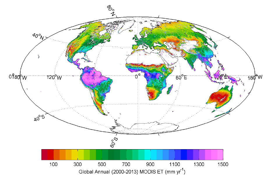
This user’s guide describes a level 4 MODIS land data product, MOD16, the global 8-day
(MOD16A2) and annual (MOD16A3) terrestrial ecosystem Evapotranspiration (ET) dataset at 0.5
km spatial resolution over the 109.03 Million km2 global vegetated land areas designed for the
MODIS sensor aboard the Aqua and Terra platforms. The MOD16 algorithm is based on the logic
of the Penman-Monteith equation which uses daily meteorological reanalysis data and 8-day
remotely sensed vegetation property dynamics from MODIS as inputs. This document is intended
to provide both a broad overview and sufficient detail to allow for the successful use of the data in
research and applications.
Please note the “MOD” prefix should be considered as referring to data sets derived from
MODIS onboard either TERRA or Aqua satellite. That is, “MOD” in this document can also be
treated as “MYD” derived from MODIS on Aqua.
1. The Algorithm, Background and Overview
Calculation of ET is typically based on the conservation of either energy or mass, or both.
Computing ET is a combination of two complicated major issues: (1) estimating the stomatal
conductance to derive transpiration from plant surfaces; and (2) estimating evaporation from the
ground surface. The MOD16 ET algorithm runs at daily basis and temporally, daily ET is the sum
of ET from daytime and night. Vertically, ET is the sum of water vapor fluxes from soil
evaporation, wet canopy evaporation and plant transpiration at dry canopy surface. Remote sensing
has long been recognized as the most feasible means to provide spatially distributed regional ET
information on land surfaces. Remotely sensed data, especially those from polar-orbiting satellites,
provide temporally and spatially continuous information over vegetated surfaces useful for
regional measurement and monitoring of surface biophysical variables affecting ET, including
albedo, biome type and leaf area index (LAI) (Los et al., 2000).
1.1 Energy Partitioning Logic
Energy partitioning at the surface of the earth is governed by the following three coupled
equations:
=
(1)
= ()
(+) (2)
==+ (3)
where H, E and A′ are the fluxes of sensible heat, latent heat and available energy for H and E;
Rnet is net radiation, G is soil heat flux; ∆S is the heat storage flux. is the latent heat of
vaporization. is air density, and CP is the specific heat capacity of air; Ts, Ta are the
aerodynamic

MOD16 User’s Guide MODIS Land Team
Version 1.6, 08/16/2018 Page 4 of 35
surface and air temperatures; ra is the aerodynamic resistance; esat, e are the water
vapour pressure
at the evaporating surface and in the air; r
s is the surface resistance to
evapotranspiration, which is
an effective resistance to evaporation from land surface and
transpiration from the plant canopy.
The psychrometric constant
is given by
=
(4)
where Ma and Mw are the molecular masses of dry air and wet air respectively and P
a the
atmospheric
p
ressure.
1.2 Penman-Monteith Logic
Developing a robust algorithm to estimate global evapotranspiration is a significant challenge.
Traditional energy balance models of ET require explicit characterization of numerous physical
parameters, many of which are difficult to determine globally. For these models, thermal remote
sensing data (e.g., land surface temperature, LST) are the most important inputs. However, using
the 8-day composite MODIS LST (the average LST of all cloud-free data in the compositing
window) (Wan et al., 2002) and daily meteorological data recorded at the flux tower, Cleugh et al.
(2007) demonstrate that the results from thermal models are unreliable at two Australian sites
(Virginia Park, a wet/dry tropical savanna located in northern Queensland and Tumbarumba, a
cool temperate, broadleaved forest in south east New South Wales). Using a combination of remote
sensing and global meteorological data, we have adapted the Cleugh et al. (2007) algorithm, which
is based on the Penman–Monteith method and calculates both canopy conductance and ET.
Monteith (1965) eliminated surface temperature from Equations (1) – (3) to give:
= + ()
+1 +
= +
+1 +
(5)
where
=(
)/
, the slope of the curve relating saturated water vapor pressure (e
sat
)
to
temperature; A′ is available energy partitioned between sensible heat and latent heat fluxes on
land
surface. VPD
=
e
sat
– e
is the air vapor pressure deficit. All inputs have been previously
defined
except for surface resistance r
s
, which is an effective resistance accounting for
evaporation from
the soil surface and transpiration from the plant canopy.
Despite its theoretical appeal, the routine implementation of the P-M equation is often
hindered by requiring meteorological forcing data (A', Ta and VPD) and the aerodynamic and
surface resistances (ra and rs). Radiation and soil heat flux measurements are needed to
determine
A′; air temperature and humidity to calculate VPD; and wind speed and surface
roughness
parameters to determine ra. Multi-temporal implementation of the P-M model at regional scales
requires routine surface meteorological observations of air temperature, humidity, solar radiation
and wind speed. Models for estimating maximum stomatal conductance including the effect of
limited soil water availability and stomatal physiology requires either a fully coupled biophysical
model such as that by Tuzet et al. (2003) or resorting to the empirical discount functions of Jarvis
MOD16 User’s Guide MODIS Land Team
Version 1.6, 08/16/2018 Page 5 of 35
(1976), which must be calibrated. Determining a surface resistance for partial canopy cover is even
more challenging with various dual source models proposed (e.g. Shuttleworth and Wallace, 1985)
to account for the presence of plants and soil.
2. The MOD16A2/MOD16A3 algorithm logic
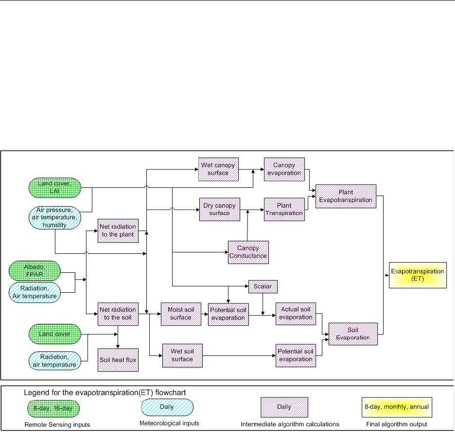
MOD16 ET algorithm is based on the Penman-Monteith equation (Monteith, 1965) as in
equation 5. Figure 2 shows the logic behind the improved MOD16 ET Algorithm for calculating
daily MOD16 ET algorithm.
Figure 2. Flowchart of the improved MOD16 ET algorithm. LAI: leaf area index; FPAR: Fraction
of
Photosynthetically Active Radiation. Net radiation calculation and the use of FPAR are detailed
in section 2.2.
2.1. Daytime and Nighttime ET
Daily ET should be the sum of daytime and nighttime ET. To separate daytime and
nighttime ET, we first obtain their air temperature which will be used in the following sections to
calculate the two ET components. To get nighttime average air temperature (Tnight), we assume
that daily average air temperature (Tavg) is the average of daytime air temperature (Tday) and
Tnight, and Tday is the average of air temperature when downward solar radiation is above 0. Thus,
= 2
(6)

MOD16 User’s Guide MODIS Land Team
Version 1.6, 08/16/2018 Page 6 of 35
The net incoming solar radiation at night is assumed to be zero. Based on the optimization theory,
stomata will close at night to prevent water loss when there is no opportunity for carbon gain
(Dawson et al., 2007). In the improved ET algorithm, at night, the stomata are assumed to close
completely and the plant transpiration through stomata is zero, except for the transpiration through
leaf boundary-layer and leaf cuticles (more details in section 2.5). Both nighttime and daytime
use the same ET algorithm except that different values at daytime and nighttime are used for the
same variable.
2.2. Soil Heat Flux
In MOD16 ET algorithm, the net incoming radiation to the land surface (Rnet) is
calculated as the equations 7 and 8 (Cleugh et al., 2007).
=(1)+ ()(273.15 +) (7)
= 1 0.26 (.)
= 0.97
where α is MODIS albedo, Rs↓ is the downward shortwave radiation, εs is surface emissivity,
εa is atmospheric emissivity, and T is air temperature in °C. At daytime, if Rnet is less than zero,
Rnet is set to be zero; at nighttime, if Rnet is less than -0.5 times of daytime Rnet, nighttime Rnet is set
as -0.5 multiplying daytime Rnet. There is no soil heat flux (G) interaction between the soil and
atmosphere if the ground is 100% covered with vegetation. Energy received by soil is the
difference between the radiation partitioned on the soil surface and soil heat flux (G).
= (8)
=
= (1 )
where A is available energy partitioned between sensible heat, latent heat and soil heat
fluxes on land surface; Rnet is the net incoming radiation received by land surface; AC is the
part of A
allocated to the canopy and ASOIL is the part of A partitioned on the soil surface. Net
radiation is partitioned between the canopy and soil surface based on vegetation cover fraction (FC),
in order to reduce numbers of inputs from MODIS datasets and to simplify the algorithm, we use
8-day 0.5 km2 MOD15A2H FPAR (the Fraction of Absorbed Photosynthetically Active Radiation)
as a surrogate of vegetation cover fraction (Los et al., 2000), FC = FPAR.
At the extremely hot or cold places or when the difference between daytime and nighttime
temperature is low (<5°C), there is no soil heat flux. The soil heat flux is estimated as:
=4.73 20.87 <,
0 <
0.39 ()> 0.39 ()

MOD16 User’s Guide MODIS Land Team
Version 1.6, 08/16/2018 Page 7 of 35
=(1 ) (9)
where G
soil
stands for the soil heat flux when F
C
=
0; T
i
means daytime or nighttime average
temperature in ℃;
Tannavg
is annual average daily temperature, and
Tmin close
is the threshold
value below which the stomata will close completely and halt plant transpiration (Table 3 . 2;
Running et al., 2004; Mu et al., 2007; Mu et al., 2011). At daytime,
G
soil day
=
0.0 if A
day
-
G
soil day
<
0.0
; at nighttime
,
G
soil night
=
A
night
+
0.5A
day
if A
day
>
0.0 and A
night
-
G
night
< -
0.5
A
day
.
2.3. Wet Surface Fraction
In the MOD16 algorithm, ET is the sum of water lost to the atmosphere from the soil
surface through evaporation, canopy evaporation from
the water intercepted by the canopy, and
transpiration from plant tissues (Fig. 2). The land surface
is covered by the plant and the bare
soil surface, and percentage of the two components is
determined by FC . Both the canopy and
the soil surface are partly covered by water under certain
conditions. The water cover fraction
(Fwet) is taken from the Fisher et al. (2008) ET model,
modified to be constrained to zero when
relative humidity (RH) is less than 70%:
=0 < 70%
70% 100% (10)
where RH is relative humidity (Fisher et al, 2008). When RH is less than 70%, 0% of the surface
is covered by water. For the wet canopy and wet soil surface, the water evaporation is calculated
as the potential evaporation as described in the next sections (2.4 and 2.6).
2.4. Evaporation from Wet Canopy Surface
Evaporation of precipitation intercepted by the canopy accounts for a substantial amount
of upward water flux in ecosystems with high LAI. When the
vegetation is covered with
water (i.e., Fwet is not zero), water evaporation from the wet canopy
surface will occur. ET from
the vegetation consists of the evaporation from the wet canopy surface
and transpiration from plant
tissue, whose rates are regulated by aerodynamics resistance and
surface resistance.
The aerodynamic resistance (rhrc , s m-1) and wet canopy resistance (rvc , s m-1) to
evaporated water on the wet canopy surface are calculated as
=1
(11)
=
4 (+273.15)
=
+

MOD16 User’s Guide MODIS Land Team
Version 1.6, 08/16/2018 Page 8 of 35
=1
where rhc (s m-1) is the wet canopy resistance to sensible heat, rrc (s m-1) is the resistance to
radiative heat transfer through air; glsh (s m-1) is leaf conductance to sensible heat per unit LAI,
gle wv (m s-1) is leaf conductance to evaporated water vapor per unit LAI, σ (W m-2 K-4) is
Stefan-Boltzmann constant.
Following Biome-BGC model (Thornton, 1998) with revision to
account for wet canopy,
the evaporation on wet canopy surface is calculated as
= + ()
+
(12)
where the resistance to latent heat transfer (rvc) is the sum of aerodynamic resistance (rhrc) and
surface resistance (rs) in equation 5.
2.5. Plant Transpiration
2.5.1. Surface Conductance to Transpiration
Plant transpiration occurs not only during daytime but also at nighttime. For many plant
species, stomatal conductance(
) decreases as vapor pressure deficit
(VPD) increases, and
stomatal conductance is further limited by both low and high temperatures
(Jarvis, 1976; Sandford
and Javis, 1986; Kawamitsu et al., 1993; Schulze et al., 1994; Leuning, 1995;
Marsden et al., 1996;
Dang et al., 1997; Oren et al., 1999; Xu et al., 2003; Misson et al.,
2004). Because high
temperatures
are often accompanied by high VPDs, we have only added constraints on stomatal
conductance
for VPD and minimum air temperature ignoring constraints resulting from high
temperature. Based on the optimization theory, stomata will close at night to prevent water loss
when
there is no opportunity for carbon gain (Dawson et al., 2007).
= () () =
0 =
(13)
The components of each terms in the above equation is calculated as below
=1
101300
+273.15
293.15 .

MOD16 User’s Guide MODIS Land Team
Version 1.6, 08/16/2018 Page 9 of 35
()=
1
<<
0
()=
1
<<
0
where CL is the mean potential stomatal conductance per unit leaf area, CL is set differently for
different biomes as shown in Table 3.2 (Kelliher et al., 1995; Schulze et al.,
1994; White et al.,
2000), m(Tmin) is a multiplier that limits potential stomatal conductance by minimum air
temperatures (Tmin), and m(VPD) is a multiplier used to reduce the potential stomatal conductance
when VPD (difference between esat and e) is high enough to reduce canopy conductance. Sub index
close indicates nearly complete inhibition (full stomatal closure) due to low Tmin and high
VPD,
and open indicates no inhibition to transpiration (Table 3.2). When Tmin is lower than the
threshold value Tmin close, or VPD is higher than the threshold VPDclose, the strong stresses from
temperature or water availability will cause stomata to close completely, halting plant transpiration.
On the other hand, when Tmin is higher than Tmin open, and VPD is lower than VPDopen, there will be
no temperature or water stress on transpiration. For Tmin and VPD falling into the range of the
upper and low limits, the corresponding multiplier will be within 0.0 to 1.0, implying a partial
stomatal closure. The multipliers range linearly from 0 (total inhibition, limiting rs) to 1 (no
inhibition) for the range of biomes are listed in a Biome Properties Look-Up Table (BPLUT)
(Table 3.2).
The reason we use the correction function rcorr for calculation of stomatal conductance is
that, the conductance through air varies with the air temperature and pressure. The prescribed
values are assumed to be given for standard conditions of 20˚C and 101300 Pa. Based on the
prescribed daily air temperature (converted to Kelvins) and an air pressure estimated from a
prescribed elevation, the prescribed standard conductances are converted to actual conductances
for the day according to Jones (1992) and Thornton (1998). Pa is calculated as a function of the
elevation (Thornton, 1998).
= 1
=
(14)
=
where LRSTD, TSTD, GSTD, RR, MA and PSTD are constant values as listed in Table 1.1
LRSTD (K m-1) is standard temperature lapse rate; TSTD (K) is standard temperature at 0.0 m
elevation; GSTD (m s-2) is standard gravitational acceleration; RR (m3 Pa mol-1 K-1) is gas law
constant; MA (kg mol-1) is molecular weight of air and PSTD (Pa) is standard pressure at 0 m
elevation.

MOD16 User’s Guide MODIS Land Team
Version 1.6, 08/16/2018 Page 10 of 35
Table 1.1 Other parameter values as used in the improved ET algorithm
LRSTD
TSTD
GSTD
RR
MA
PSTD
(K m-1)
(K)
(m s-2)
(m3 Pa mol-1 K-1)
(kg mol-1)
(Pa)
0.0065
288.15
9.80665
8.3143
28.9644e-3
101325.0
Canopy conductance (Cc) to transpired water vapor per unit LAI is derived from stomatal
and cuticular
conductances in parallel with each other, and both in series with leaf boundary layer
conductance
(Thornton, 1998; Running & Kimball, 2005). In the case of plant transpiration,
surface conductance is equivalent to the canopy conductance (CC), and hence surface resistance
(rs) is the inverse of canopy conductance (CC).
=(
+)
++ (1) (> 0, (1)> 0)
0 (= 0, (1)= 0)
(15)
=
=
=1
where the subscript i means the variable value at daytime and nighttime; GCU is leaf cuticular
conductance; is leaf boundary-layer conductance; is cuticular conductance per unit LAI,
set as a constant value of 0.00001 (m s-1) for all biomes; is leaf conductance to sensible heat
per unit LAI, which is a constant value for each given biome (Table 3.2).
2.5.2. Aerodynamic Resistance
The transfer of heat and water vapor from the dry canopy surface into the air above the canopy
is determined by the aerodynamic resistance (ra). ra is calculated as a parallel resistance to
convective (rh) and radiative (rr) heat transfer following Biome-BGC model (Thornton, 1998).
=
+
=1
(16)
=
4 (+273.15)
where glbl (m s-1) is leaf-scale boundary layer conductance, whose value is equal to leaf
conductance to sensible heat per unit LAI (glsh (m s-1) as in section 2.4), and σ (W m-2 K-4) is
Stefan-Boltzmann constant.
2.5.3. Plant Transpiration
Finally, the plant transpiration (AEtrans) is calculated as

MOD16 User’s Guide MODIS Land Team
Version 1.6, 08/16/2018 Page 11 of 35
= + ()
(1 )
+1 +
(17)
where r
a is the aerodynamic resistance calculated from equation 5.
= (1 )
+ (18)
with α = 1.26.
2.6. Evaporation from Soil Surface
The soil surface is divided into the saturated surface covered with water and the moist
surface by Fwet. The soil evaporation includes the potential evaporation from the saturated soil
surface and evaporation from the moist soil surface. The total aerodynamic resistance to vapor
transport (rtot) is the sum of surface resistance (rs) and the aerodynamic resistance for vapor
transport (rv) such that rtot = rv + rs (van de Griend & Owe, 1994; Mu et al., 2007). We assume that
rv (s m-1) is equal to the aerodynamic resistance (ra: s m-1) in Equation 5 since the values of rv
and ra are usually very close (van de Griend & Owe, 1994). In the MOD16 ET algorithm, the
rhs is assumed to be equal to boundary layer resistance, which is calculated in the same way as
total aerodynamic resistance (rtot) (Thornton, 1998) only that, rtotc is not a constant. For a given
biome type, there is a maximum (rblmax) and a minimum value (rblmin) for rtotc, and rtotc is a function
of VPD.
= (19)
=
()()
<<
where rcorr is the correction for atmospheric temperature and pressure (equation 13) above
mentioned. The values of rblmax and rblmin, VPDopen (when there is no water stress on transpiration)
and VPDclose (when water stress causes stomata to close almost completely, halting plant
transpiration) are parameterized differently for different biomes and are listed in Table 3.2.
The aerodynamic
resistance at the soil surface (ras) is parallel to both the resistance to
convective heat transfer (rhs:
s m-1) and the resistance to radiative heat transfer (rrs: s m-1)
(Choudhury and DiGirolamo, 1998), such that
=
+
= (20)
=
4 (+273.15)

MOD16 User’s Guide MODIS Land Team
Version 1.6, 08/16/2018 Page 12 of 35
The actual soil evaporation () is calculated in equation 21 using potential soil evaporation
( ) and soil moisture constraint function in the Fisher et al. (2008) ET model. This
function is based on the complementary hypothesis (Bouchet, 1963), which defines land-
atmosphere interactions from air VPD and relative humidity (RH, %).
= + (1 )
+
= + (1 )
(1)
+
(21)
= +
100
with β = 250.
2.7. Total Daily Evapotranspiration
The total daily ET is the sum of evaporation from the wet canopy
surface, the transpiration
from the dry canopy surface and the evaporation from the soil surface.
The total daily ET and
potential ET(λEPOT) are calculated as in equation 22.
= ++ (22)
= + + +
Combination of ET with the potential ET can determine environmental water stress and detect the
intensity of drought.
2.8. Updates after Publication of RSE Paper by Mu et al. (2011)
The MOD16 products are generated based on the MOD16 algorithm in Mu et al.'s 2011
RSE paper. Since the publication, Dr. Mu have updated the product to fix some issues and these
updates have been implemented in the operational code.
1. Issue of negative ET and PET values for some 8-day and monthly data.
In the previous product, we allowed the net incoming daytime radiation to be negative.
Only MERRA daytime downward solar radiation, daytime actual vapor pressure, daytime
temperature, daily average and minimum temperatures are used as meteorological inputs. The
outgoing and incoming longwave radiation is calculated as in Mu et al.'s 2011 RSE paper. In the
updated product, the nighttime actual vapor pressure, nighttime temperature, outgoing and
incoming longwave radiation are from MERRA directly. If daytime < 0; daytime = 0.
In the MOD16 ET algorithm, when we calculated the soil heat flux, we didn't constrain the
soil heat flux. The net radiation to the bare ground is difference between the fraction of the net
incoming radiation reaching to the ground surface (Rground) and the soil heat flux (G). In certain
MOD16 User’s Guide MODIS Land Team
Version 1.6, 08/16/2018 Page 13 of 35
cases, G is higher than Rground, resulting in negative soil evaporation. In the updated product,
We set limit to G. For daytime and :
() < 0; =
Whereas for nighttime and :
() < 0.5 ; = + 0.5
2. Issue of no valid MODIS surface albedo values throughout the year for vegetated pixels
due to high frequency of cloudiness.
In the improved MOD16. For example, no single valid MODIS albedo can be found
throughout an entire year over rainforests of west Africa due to severe and constant cloudiness. In
the update version, we specify an albedo value of 0.4 for the pixels, a typical value for nearby
rainforests with valid albedo values.
3. Operational Details of MOD16 and Primary Uncertainties in the MOD16
Logic
A number of issues are important in implementing this algorithm. This section discusses
some of the assumptions and special issues involved in development of the input variables, and
their influence on the final ET estimates.
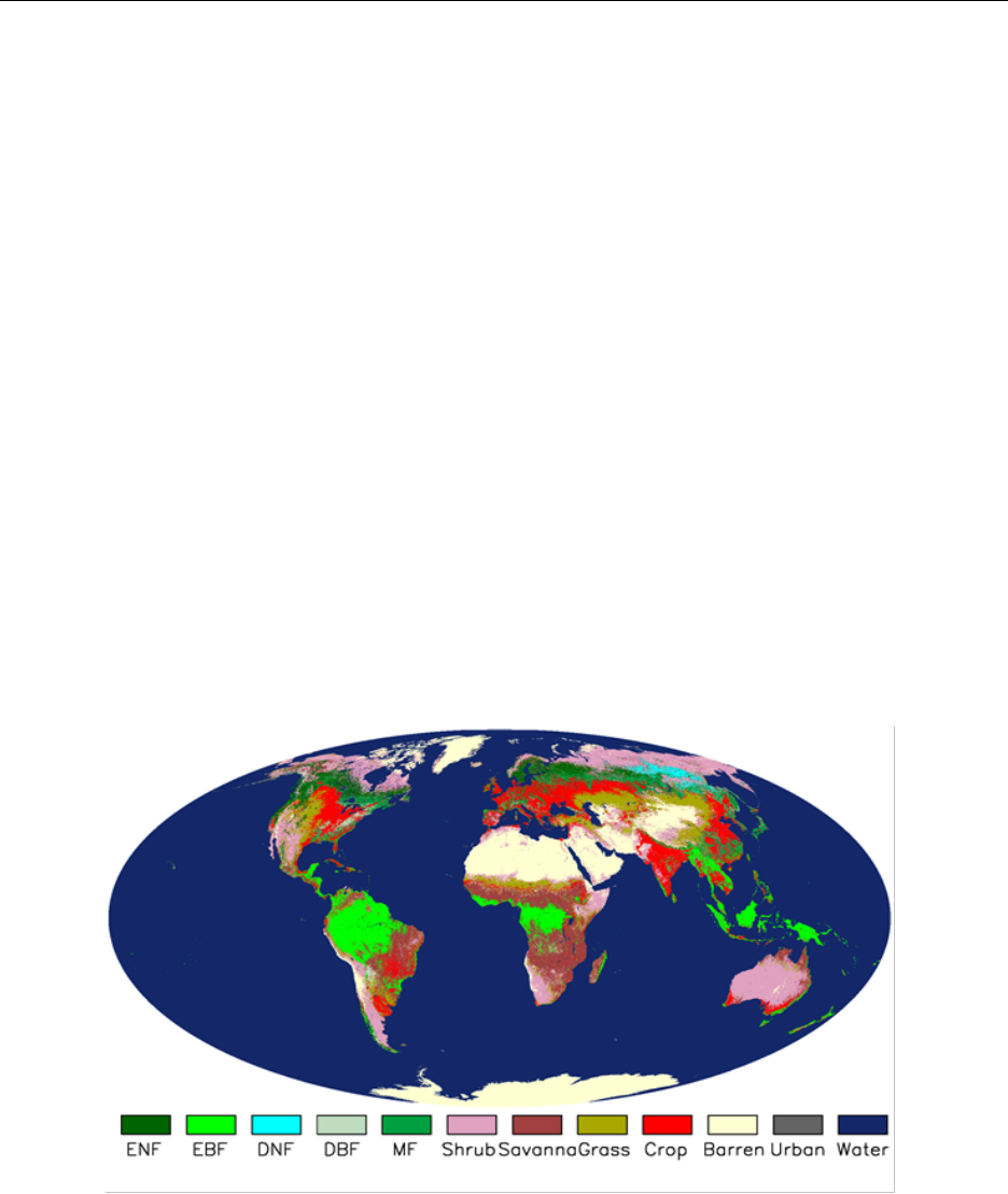
3.1. Dependence on MODIS Land Cover Classification MCDLCHKM
Figure 3.1. Collection5 1-km MODIS ET used land cover type 2 in 1-km Collection4
MOD12Q1 dataset. Whereas Collection6 operational 500-m MODIS ET is using land cover type
1 in Collection5.1 500-m MCDLCHKM which is a 3-year smoothed MODIS land cover data set.
This figures shows land cover types from the Collection4 MOD12Q1 dataset: Evergreen
Needleleaf Forest (ENF), Evergreen Broadleaf Forest (EBF), Deciduous Needleleaf Forest (DNF),
Deciduous Broadleaf Forest (DBF), Mixed forests (MF), Closed Shrublands (CShrub), Open
Shrublands (OShrub), Woody Savannas (WSavanna), Savannas (Savanna), grassland (Grass),
and Croplands (Crop). Note that in this figure, we combined CShrub and OShrub into Shrub, and

MOD16 User’s Guide MODIS Land Team
Version 1.6, 08/16/2018 Page 14 of 35
WSavanna and Savannas into Savanna. Globally, Collection5.1 500-m MCDLCHKM has a
similar spatial pattern to this image.
One of the first MODIS products used in the MOD16 algorithm is the Land Cover Product.
For the previous Collection5 1-km MODIS ET, the 1-km land cover type 2 in a frozen version of
the Collection4 MOD12Q1 was used. However, for the operational Collection 6 500-m MODIS
ET, a 3-year smoothed land cover data set, land cover type 1 in the Collection5.1 500-m
MCDLCHKM, is being used. The importance of this product cannot be overstated as the MOD16
algorithm relies heavily on land cover type through use of the BPLUT. The land cover type 1
created by 500-m MCDLCHKM is a 17-class IGBP (International Geosphere-Biosphere
Programme) land cover classification map (Running et al. 1994, Belward et al. 1999, Friedl et al.
2010) (Table 3.1). Figure 3.1 shows the Collection4 1-km MOD12Q1 dataset used by the
Collection5 MODIS ET. Globally, Collection5.1 500-m MCDLCHKM has a very similar spatial
pattern to this image though it may have a different land cover type for a given pixel.
3.1.1. The BPLUT and constant biome properties
Arguably, the most significant assumption made in the MOD16 logic is that biome-specific
physiological parameters do not vary with space or time. These parameters are outlined in the
BPLUT (Table 3.2) within the MOD16 algorithm. The BPLUT constitutes the physiological
framework for controlling simulated ET. These biome-specific properties are not differentiated
for different expressions of a given biome, nor are they varied at any time during the year. In other
words, a semi-desert grassland in Mongolia is treated the same as a tallgrass prairie in the
Midwestern United States. Likewise, a sparsely vegetated boreal evergreen needleleaf forest in
Canada is functionally equivalent to its coastal temperate evergreen needleleaf forest counterpart.
Table 3.1. The land cover types used in the MOD16 Algorithm.
Land Cover Type 1 in 500-m MCDLCHKM
Class Value
Class Description
0
Water
1
Evergreen Needleleaf Forest
2
Evergreen Broadleaf Forest
3
Deciduous Needleleaf Forest
4
Deciduous Broadleaf Forest
5
Mixed Forest
6
Closed Shrubland
7
Open Shrubland
8
Woody Savanna
9
Savanna
10
Grassland
12
Cropland
13
Urban or Built-Up
16
Barren or Sparsely Vegetated
254
Unclassified
255
Missing Data

Table 3.2. Biome-Property-Look-Up-Table (BPLUT) for MODIS ET algorithm with NCEP-DOE reanalysis II and the Collection 6
FPAR/LAI/Albedo as inputs. The full names for veget land cover classification system in 500-m MCDLCHKM dataset (fieldname:
Land_Cover_Type_1) are, Evergreen Needleleaf Forest (ENF), Evergreen Broadleaf Forest (EBF), Deciduous Needleleaf Forest (DNF),
Deciduous Broadleaf Forest (DBF), Mixed forests (MF), Closed Shrublands (CShrub), Open Shrublands (OShrub), Woody Savannas
(WSavanna), Savannas (Savanna), Grassland (Grass), and Croplands (Crop). Note this table has been updated since publication of RSE
paper by Mu et al. (2011), and please refer to section 2.8 for details.
VEG_LC
ENF
EBF
DNF
DBF
MF
CShrub
OShrub
WSavanna
Savanna
Grass
Crop
Tmin
close
(C)
-8.00
-8.00
-8.00
-6.00
-7.00
-8.00
-8.00
-8.00
-8.00
-8.00
-8.00
Tmin
open
(C)
8.31
9.09
10.44
9.94
9.50
8.61
8.80
11.39
11.39
12.02
12.02
VPD
open
(Pa)
650.0
1000.0
650.0
650.0
650.0
650.0
650.0
650.0
650.0
650.0
650.0
VPD
close
(Pa)
3000.0
4000.0
3500.0
2900.0
2900.0
4300.0
4400.0
3500.0
3600.0
4200.0
4500.0
gl
sh
(m s-1)
0.01
0.01
0.01
0.01
0.01
0.02
0.02
0.04
0.04
0.02
0.02
gl
e wv
(m s-1)
0.01
0.01
0.01
0.01
0.01
0.02
0.02
0.04
0.04
0.02
0.02
g
cu
(m s-1)
0.00001
0.00001
0.00001
0.00001
0.00001
0.00001
0.00001
0.00001
0.00001
0.00001
0.00001
CL (m s-1)
0.00240
0.00240
0.00240
0.00240
0.00240
0.00550
0.00550
0.00550
0.00550
0.00550
0.00550
rblmin (s m-1)
60.0
60.0
60.0
60.0
60.0
60.0
60.0
60.0
60.0
60.0
60.0
rblmax (s m-1)
95.0
95.0
95.0
95.0
95.0
95.0
95.0
95.0
95.0
95.0
95.0
MOD16 User’s Guide MODIS Land Team
Version 1.6, 08/16/2018 Page 15 of 35

MOD16 User’s Guide MODIS Land Team
Version 1.6, 08/16/2018 Page 16 of 35
3.2 Leaf area index, fraction of absorbed photosynthetically active radiation and
albedo
The FPAR/LAI product is an 8-day composite product. The MOD15 compositing
algorithm uses a simple selection rule whereby the maximum FPAR (across the eight days) is
chosen for the inclusion as the output pixel. The same day chosen to represent the FPAR measure
also contributes the current pixel’s LAI value. This means that although ET is calculated daily, the
MOD16 algorithm necessarily assumes that leaf area and FPAR do not vary during a given 8-day
period. Compositing of LAI and FPAR is required to provide an accurate depiction of global leaf
area dynamics with consideration of spectral cloud contamination, particularly in the tropics.
The MCD43A2/A3 albedo products are 16-day moving daily products too. Both Terra and
Aqua data are used in the generation of this product, providing the highest probability for quality
input data and designating it as an "MCD," meaning "Combined," product. Version-6
MODIS/Terra+Aqua BRDF/Albedo products are Validated Stage 1, indicating that accuracy has
been estimated using a small number of independent measurements obtained from selected
locations and time periods and ground-truth/field program efforts. Although there may be later
improved versions, these data are ready for use in scientific publications.
3.2.1. Additional Cloud/Aerosol Screening
The 8-day MOD15A2H and daily MCD43A3 are still contaminated by clouds and/or
aerosols in certain regions and times of year. As a result, in regions with higher frequencies of
cloud cover, such as tropical rain forests, values of FPAR and LAI will be greatly reduced and the
albedo signal dramatically increased. To distinguish between good quality and contaminated data,
MOD15A2H and MCD43A3 contain Quality Control (QC) fields, enabling users to determine
which pixels are suitable for further analysis. The use of contaminated FPAR, LAI or albedo inputs
will produce incorrect ET estimates. Thus for NASA’s operational MOD16 dataset, users should
be cautious when use the data and contaminated MOD16 data sets should be excluded from
analysis. In this case, QC data field should be used to distinguish uncontaminated or unreliable
MOD16 pixels for the same data period. Only for the reprocessed and improved MOD16, users
may ignore QC because the contaminated MODIS inputs to MOD16 have been temporally filled,
resulting in an improved MOD16. The following describes the method we employed for the
improved MOD16.
The following screening and gap-filling processes are only applied to the improved MOD16.
In the early of each year when the previous full yearly MOD15A2H/MCD43A3 are available for
reprocess (also see section 6.3).
To improve the MOD16 data product, we solved this problem related to
MOD15A2H/MCD43A3 inputs by removing poor quality FPAR/LAI/Albedo data based on the
QC label for every pixel. If, for example, any LAI/FPAR pixel did not meet the quality screening
criteria, its value is determined through linear interpolation between the previous period’s value
and that of the next period to pass the screening process. Contaminated MOD15A2H/MCD43A3
was improved as the result of the filling process. However, there are some unusual 8-day periods
with lower FPAR and LAI but good QC labels. In spite of this, we have to depend on QC label

MOD16 User’s Guide MODIS Land Team
Version 1.6, 08/16/2018 Page 17 of 35
because this is the only source of quality control. Improved MOD15A2H/MCD43A3 leads to
improvements of MOD16.
3.3. GMAO daily meteorological data
The MOD16 algorithm computes ET at a daily time step. This is made possible by the
daily
meteorological data, including average and minimum air temperature, incident PAR and
specific
humidity, provided by NASA’s Global Modeling and Assimilation Office (GMAO or MERRA
GMAO), a branch of NASA (Schubert et al. 1993). These data, produced every six
hours, are
derived using a global circulation model (GCM), which incorporates both ground and
satellite-
based observations. These data are distributed at a resolution of 0.5° x 0.6° (MERRA GMAO) or
1.00° x 1.25° (note that resolution may become finer with updates of GMAO system at NASA) in
contrast to the 0.5 km gridded MOD16 outputs. It is
assumed that the coarse resolution
meteorological data provide an accurate depiction of ground conditions and are homogeneous
within the spatial extent of each cell.
One major problem is the inconsistency in spatial resolution between half-degree GMAO/NASA
meteorological data and 0.5 km MODIS pixel. We solved the problem by spatially smoothing
meteorological data to 0.5 km MODIS pixel level. For the problem arising from coarse spatial
resolution daily GMAO data, we use spatial interpolation to enhance meteorological inputs. The
four GMAO cells nearest to a given 0.5 km MODIS pixel are used in the interpolation algorithm.
There are two reasons for choosing four GMAO cells per 0.5 km MODIS pixel: (1) this will not
slow down the computational efficiency of creating MOD16, which is a global product, and (2) it
is more reasonable to assume no elevation variation within four GMAO cells than more GMAO
cells. Although there are many formulae for non-linear spatial interpolation, for simplicity, we
use a cosine function because the output value can be constrained between 0 and 1. This function
still could not effectively boundary lines in a MOD16 image, and thus we utilized a modified
cosine function of the form:
))/)(2/((cos
max
4
ddD
ii
π
=
4,3,2,1=i
(23)
where, Di is the non-linear distance between the 0.5 km MODIS pixel and any one of four
surrounding GMAO cells; di is the great-circle distance between the 0.5 km pixel and the same
GMAO cell; and dmax is the great-circle distance between the two farthest GMAO cells of the four
being used. This ensures that Di = 1 when di = 0, and Di = 0 when di = dmax.
Based on the non-linear distance (Di), the weighted value Wi can be expressed as
∑
=
=
4
1
/
iiii DD
W
, (24)
and therefore, for a given pixel, the corresponding smoothed value
V
(i.e., interpolated Tmin,
Tavg, VPD, SWrad) is
MOD16 User’s Guide MODIS Land Team
Version 1.6, 08/16/2018 Page 18 of 35
∑
=
=
4
1
)(
iiiVWV
(25)
Theoretically, this GMAO spatial interpolation can improve the accuracy of
meteorological data for each 0.5 km pixel because it is unrealistic for meteorological data to
abruptly change from one side of GMAO boundary to the other. To explore the above question,
we use observed daily weather data from World Meteorological Organization (WMO) daily
surface observation network (>5000 stations) to compare changes in Root Mean Squared Error
(RMSE) and Correlation (COR) between the original and enhanced DAO data. As a result of the
smoothing process, on average, RMSE is reduced and COR increased for 72.9% and 84% of the
WMO stations, respectively, when comparing original and enhanced DAO data to WMO
observations for 2001 and 2002. Clearly, the nonlinear spatial interpolation significantly improves
GMAO inputs for most stations, although for a few stations, interpolated GMAO accuracy may be
reduced due to the inaccuracy of GMAO in these regions. (Zhao et al. 2005, 2006)
4. Validation of MOD16
To validate the MOD16 algorithm, we used the observed latent heat flux for 46 field-based
eddy covariance flux towers, global
232 watersheds, as well as global results over the past 11
years (2000 to 2010). We cut out the input MODIS data for the 3 x 3 1-km2 pixels surrounding
each tower. We
drove the MOD16 ET algorithm with both tower observed meteorological data and
global GMAO meteorological data. We got the average ET estimates over those of the 3 x 3 1-km2
pixels where
the tower actual vegetation type is the same as MODIS land cover. Then we compared
the
ET estimates with the tower ET observations. For each of the seven biome types among the
46 flux towers except for CSH and OSH since there is only one tower with fewer than
365 measurements for each of them, we chose one tower to show the performance of MOD16
ET
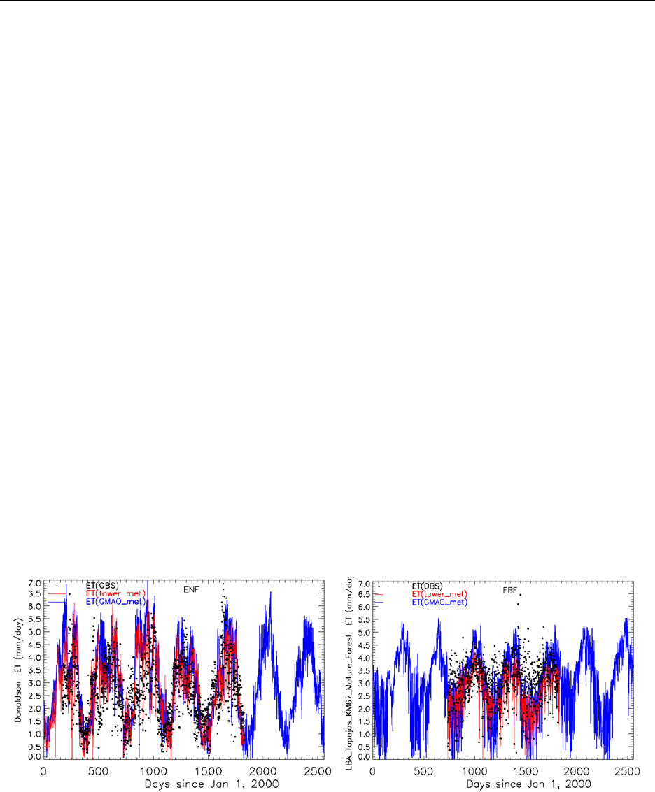
algorithm (Fig. 4.1).
Figure 4.1. The ET measurements (black dots, OBS), the ET estimates driven by flux tower measured
meteorological data (red lines) and GMAO meteorological data (blue lines) over 2000-2006 at seven tower
sites, Donaldson (a) and LBA Tapajos KM67 Mature Forest (b).
a
b

MOD16 User’s Guide MODIS Land Team
Version 1.6, 08/16/2018 Page 19 of 35
The average daily ET biases between ET observations and ET estimates across the 46
towers are -0.11 kg/m2/day driven by tower meteorological data and -0.02 kg/m2/day driven by
GMAO meteorological data. The average mean absolute errors (MAE) are 0.33 kg/m2/day (tower-
specific meteorology) and 0.31 kg/m2/day (GMAO meteorology). The MAE values are 24.6% and
24.1% of the ET measurements, within the 10-30% range of the accuracy of ET observations
(Courault et al. 2005; Jiang et al. 2004; Kalma et al. 2008).
5. Practical Details for downloading MOD16 Data
All MODIS land data products are distributed to global users from the USGS Land
Processes Distributed Active Archive Center (USGS LP DAAC), found here:
https://lpdaac.usgs.gov/
Specific details about the MODIS land products can be found here:
https://lpdaac.usgs.gov/dataset_discovery/modis
including details about sensor spectral bands, spatial/temporal resolution, platform overpass
timing, datafile naming conventions, tiling formats, processing levels and more.
When this document is being written, MODAPS at NASA is testing the operational
Collection6 MOD16 code and 500m MOD16 data will be released to the public through the USUS
LP DAAC soon (https://lpdaac.usgs.gov/data_access ).
The long-term consistent improved global Collection5 1-km MOD16 from year of 2000 to
the previous year can be downloaded at NTSG at site
http://www.ntsg.umt.edu/project/mod16#data-product
6. MOD16 Data Description and Process
6.1. Description and Process of MOD16 Data Files
There are two major MOD16 data sets, 8-day composite MOD16A2 and annual composite
MOD16A3. Both MOD16A2 and MOD16A3 are stored in HDFEOS2 scientific data file format
(http://hdfeos.org/software/library.php). HDFEOS2 file format is an extension of HDF4 by
adding geo-reference, map projection, and other key meta data information to HDF4 format
(https://support.hdfgroup.org/products/hdf4/) to facilitate users to use satellite data products from
NASA’s Earth Observing System (EOS) projects. Since MOD16 is a level 4 EOS data product,
the grid data sets are saved in Sinusoidal (SIN) map projection, an equal-area map projection, with
an earth radius of 6371007.181 meters (Note the inversed lat/lon are in WGS84 datum). The
MODIS high-level data sets divide the global SIN into many chunks, so-called 10-degree tiles
(https://modis-land.gsfc.nasa.gov/MODLAND_grid.html). There are 317 land tiles, and among
which, 300 tiles (286 tiles for the Collection5) located within latitude of 60°S and 90°N (90°N for

MOD16 User’s Guide MODIS Land Team
Version 1.6, 08/16/2018 Page 20 of 35
the Collection5) have vegetated land pixels. Therefore, for each 8-day Collection6 MOD16A2
and yearly MOD16A3, there are 300 land tiles globally if there are no missing tiles.
When MODIS updates MOD16 from the Collection5 to Collection6, the spatial resolution
has increased from nominal 1-km (926.62543313883 meters) to 500m (463.312716569415
meters), to be consistent with changes in the spatial resolution of a major input to MOD16, the 8-
day MOD15A2H.
For users don’t know how to handle and process MODIS high-level data products, we
suggest users use free or commercial software tools, such as MODIS Reprojection Tool (MRT)
(https://lpdaac.usgs.gov/tools/modis_reprojection_tool )
, HDF-EOS to GeoTIFF Conversion Tool (HEG) (http://hdfeos.org/software/heg.php ), or
MODIS toolbox in ArcMap (https://blogs.esri.com/esri/arcgis/2011/03/21/global-
evapotranspiration-data-accessible-in-arcmap-thanks-to-modis-toolbox/) to handle MOD16.
6.2. Description of MOD16 Date Sets
6.2.1. MOD16A2
Table 6.1 lists science data sets in the 8-day MOD16A2. ET_500m and potential ET (PET),
PET_500m, are the summation of 8-day total water loss through ET (0.1 kg/m2/8day), whereas
the associated latent heat fluxes and its potential, LE_500m and PLE_500m, are the average total
energy over a unit area for a unit day during the composite 8-day period (10000 J/m2/day). But be
cautious that the last 8-day (MOD16A2.A20??361.*.hdf) of each year is not 8-day but either 5-
day or 6-day depending on normal or leap year.
As listed in Table 6.1, for valid data (Valid_data with the valid range) of MOD16A2, the
real value (Real_value) of each data set (ET, LE, PET or PLE) in the corresponding units (kg/m2/8d
or J/m2/d) can be calculated using the following equation,
Real_value = Valid_data * Scale_Factor (26)
Table 6.1. The detailed information on science data sets in MOD16A2
Data Sets
Meaning
Units
Date
Type
Valid Range
Scale
Factor
ET_500m
8-day total ET
kg/m2/8d
int16
-32767 ~ 32760
0.1
LE_500m
8-day average LE
J/m2/d
int16
-32767 ~ 32760
10000
PET_500m
8-day total PET
kg/m2/8d
int16
-32767 ~ 32760
0.1
PLE_500m
8-day average PLE
J/m2/d
int16
-32767 ~ 32760
10000
ET_QC_500m
Quality Control
none
uint8
0 ~ 254
none
All data sets in MOD16A2, except Quality Control (QC) data field, ET_QC_500m, have
valid value ranging from -32767 to 32760 and are saved in signed 2-byte short integer (int16).
Though data attributes list just one _FillValue: 32767 in the head file of MOD16A2 file, there are,
in fact, 7 fill values listed below for non-vegetated pixels, which we didn’t calculate ET.

MOD16 User’s Guide MODIS Land Team
Version 1.6, 08/16/2018 Page 21 of 35
32767 = _Fillvalue
32766 = land cover assigned as perennial salt or Water bodies
32765 = land cover assigned as barren,sparse veg (rock,tundra,desert)
32764 = land cover assigned as perennial snow,ice.
32763 = land cover assigned as "permanent" wetlands/inundated marshland
32762 = land cover assigned as urban/built-up
32761 = land cover assigned as "unclassified" or (not able to determine)
The QC data layer, ET_QC_500m, directly inherits the QC data field, FparLai_QC, from the
corresponding MOD15A2 of the same 8-day. Detailed information of bitfields in 8 bitword is the
same as that from MOD15A2, as detailed below.
Data Field Name: ET_QC_500m
BITS BITFIELD
-------------
0,0 MODLAND_QC bits
'0' = Good Quality (main algorithm with or without saturation)
'1' = Other Quality (back-up algorithm or fill values)
1,1 SENSOR
'0' = Terra
'1' = Aqua
2,2 DEADDETECTOR
'0' = Detectors apparently fine for up to 50% of channels 1,2
'1' = Dead detectors caused >50% adjacent detector retrieval
3,4 CLOUDSTATE (this inherited from Aggregate_QC bits {0,1} cloud state)
'00' = 0 Significant clouds NOT present (clear)
'01' = 1 Significant clouds WERE present
'10' = 2 Mixed cloud present on pixel
'11' = 3 Cloud state not defined,assumed clear
5,7 SCF_QC (3-bit, (range '000'..100') 5 level Confidence Quality score.
'000' = 0, Main (RT) method used, best result possible (no saturation)
'001' = 1, Main (RT) method used with saturation. Good,very usable
'010' = 2, Main (RT) method failed due to bad geometry, empirical algorithm used
'011' = 3, Main (RT) method failed due to problems other than geometry, empirical algorithm
used
'100' = 4, Pixel not produced at all, value coudn't be retrieved (possible reasons: bad L1B data,
unusable MOD09GA data)
For non-improved NASA’s operational MOD16A2, we suggest users at least exclude cloud-
contaminated cells. For the improved and reprocessed MOD16A2, users may ignore QC data layer
because cloud-contaminated LAI/FPAR gaps have been temporally filled before calculating ET

MOD16 User’s Guide MODIS Land Team
Version 1.6, 08/16/2018 Page 22 of 35
(Mu e al., 2007, also see previous section 3.2.1 and following 6.3). QC just denotes if filled
LAI/FPAR were used as inputs. Because current operational MOD16A2 didn’t calculate ET when
the input MODIS data are unreliable, users may also ignore QC data layers for the NASA’s
operational MOD16 but just use pixels with values within the valid range.
6.2.2. MOD16A3
Table 6.2 lists science data sets in annual MOD16A3. ET_500m and PET_500m are the
summation of total daily ET/PET through the year (0.1 kg/m2/year) whereas LE and PLE are the
corresponding average total latent energy over a unit area for a unit day (10000 J/m2/day) through
the year. LE_500m and PLE_500m have the same unit, data type (signed 2-byte short int16), valid
range and fill values as those listed above for the 8-day MOD16A2; whereas annual ET_500m and
PET_500m are saved in unsigned 2-byte short integer (uint16) with valid range from 0 to 65528.
Similar to MOD16A2, as listed in Table 6.2, for valid data (Valid_data with the valid range)
of MOD16A3, the real value (Real_value) of each data set (ET, LE, PET or PLE) in the
corresponding units (kg/m2/yr or J/m2/d) can be calculated using the following equation,
Real_value = Valid_data * Scale_Factor (27)
Though data attributes list one _FillValue: 65535 in the HDFEOS MOD16A3 file, there are,
in fact, 7 fill values as listed below for non-vegetated pixels without ET calculations.
65535 = _Fillvalue
65534 = land cover assigned as perennial salt or Water bodies
65533 = land cover assigned as barren,sparse veg (rock,tundra,desert)
65532 = land cover assigned as perennial snow,ice.
65531 = land cover assigned as "permanent" wetlands/inundated marshland
65530 = land cover assigned as urban/built-up
65529 = land cover assigned as "unclassified" or (not able to determine)
Table 6.2. The detailed information on science data sets in MOD16A3
Data Sets
Meaning
Units
Date
Type
Valid Range
Scale
Factor
ET_500m
annual sum ET
kg/m2/yr
uint16
0 ~ 65528
0.1
LE_500m
annual average LE
J/m2/d
int16
0 ~ 32760
10000
PET_500m
annual sum PET
kg/m2/yr
uint16
0 ~ 65528
0.1
PLE_500m
annual average PLE
J/m2/d
int16
0 ~ 32760
10000
ET_QC_500m
Quality Assessment
Percent (%)
uint8
0 ~ 100
none
QC data field in annual MOD16A3, ET_QC_500m, is different from most MODIS QC
data sets because it is not bitfields but a more meaningful QC assessment for annual composite
values. We used the method proposed by Zhao et al. (2005) to define annual ET QC as
ET_QC_500m = 100.0 x NUg/Totalg (28)

MOD16 User’s Guide MODIS Land Team
Version 1.6, 08/16/2018 Page 23 of 35
where NUg is the number of days during growing season with filled MODIS 500m LAI inputs to
MOD16 due to missing or unfavorable atmospheric contaminated MODIS LAI (hence FPAR) if
improvement reprocess is employed. Totalg is total number of days in the growing season. The
growing season is defined as all days with Tmin above the value where stomata close as in the
BPLUT.
The data type of ET_QC_500m is unsigned 1-byte integer (uint8) with valid range from 0
to 100. For vegetated land pixels, if ET_QC_500m has no spatial variations, it will imply the
MOD16A3 is the NASA’s operational data product, but not the improved by reprocessing because
frequency of cloud contaminations varies with space. Though data attributes list one _FillValue:
255 in the HDFEOS MOD16A3 file, there are, in fact, 7 fill values as listed below for non-
vegetated pixels.
255 = _Fillvalue
254 = land cover assigned as perennial salt or Water bodies
253 = land cover assigned as barren,sparse veg (rock,tundra,desert)
252 = land cover assigned as perennial snow,ice.
251 = land cover assigned as "permanent" wetlands/inundated marshland
250 = land cover assigned as urban/built-up
249 = land cover assigned as "unclassified" or not able to determine
6.3. Evaluation of NASA Operational MOD16 with NTSG Gap-filled
The following subsection 1) reveals the differences between NASA operational and NTSG gap-
filled MOD16 by showing one 8-day global browser of ET in Figure 6.1; 2) demonstrates close
global agreements between NASA operational Collection6 MOD16A2, MYD16A2 and NTSG
Collection5 gap-filled data. Based on our evaluation, we conclude that NASA operational
Collection6 MOD16A2 and MYD16A3 are ready for users to apply the data to studies of global
terrestrial water and energy cycles and environmental changes.
As mentioned in the previous sections, NASA operational MOD16A2 contains data gaps
mainly due to cloudiness or snow cover, which obscures the ground information observed by
MODIS and results in unrealistic biophysical variables derived from MODIS, the inputs to
MOD16 (Figure 6.1). The reprocessed MOD16 dataset from Numerical Terradynamic Simulation
Group (NTSG) at University of Montana (UMT) is a gap-filled dataset which have solved the issue
of cloud- or snow-contaminations by temporally gap-filling the biophysical variables using the
data from the uncontaminated data prior and post the contaminated periods (Zhao et al., 2005; Mu
et al., 2007; Mu et al., 2011).
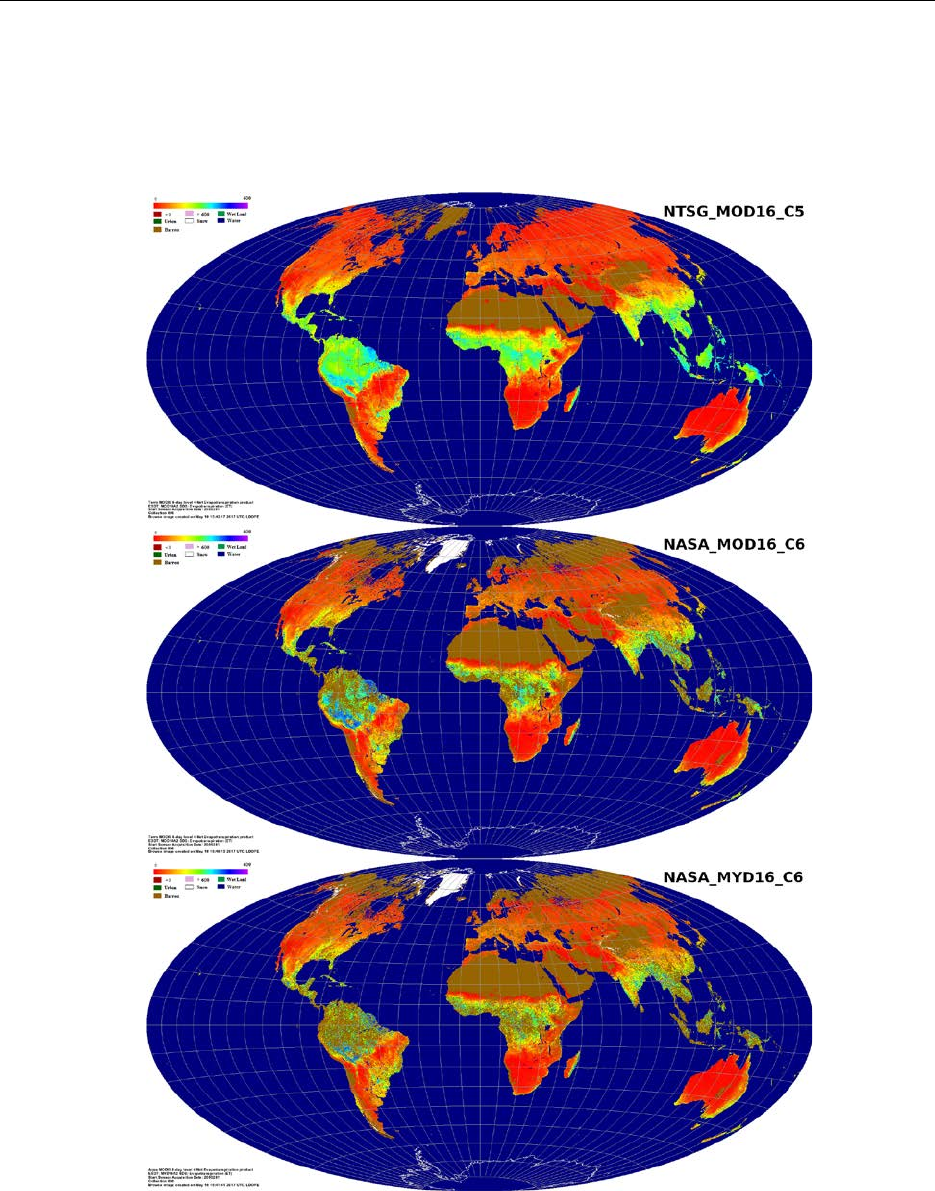
Figure 6.1 shows an 8-day (2008281, early October) MODIS ET from gap-filled NTSG
Collection5 (C5) and operational Collection (C6) NASA MOD16 and MYD16. It clearly shows
large areas with data gaps which are mainly caused by cloudiness or snow cover. Currently, fill
value denoting “Barren or sparsely vegetated” are used as value for these data gaps with vegetated
pixels in operational data set which is shown in bronze color in the image. In tropical rainforests,
there are large areas of data gaps caused by cloudiness in the NASA operational MOD16A2 8-day
ET datasets, similar phenomena occur to the other three variables: LE, PET and PLE (not shown).
MOD16 User’s Guide MODIS Land Team
Version 1.6, 08/16/2018 Page 24 of 35
The main reason for more data gaps in MYD16 than in MOD16 is the difference in the local
overpass time between TERRA and Aqua satellite. TERRA’s overpass time is in the morning
whereas Aqua in the afternoon, and convection is much stronger in the afternoon when the land
surface is warmer than in the morning when it is cooler. Stronger convection potentially can
induce more cloudiness.
Figure 6.1. Comparison of MOD16A2 for an 8-day of 2008281 (Oct 7th through Oct 14th) between
NTSG Collection5 gap-filled and NASA operational Collection6 with data gaps due to cloudiness
or snow cover.

MOD16 User’s Guide MODIS Land Team
Version 1.6, 08/16/2018 Page 25 of 35
We evaluated the NASA C6 operational MOD16 by comparing it with gap-filled NTSG
C5 just for commonly valid pixels from both data sets. Because C6 and C5 have different versions
of MODIS inputs, such as MODIS land cover, LAI/FPAR, and surface albedo, and the two also
use different versions of daily meteorological data sets (operational GMAO for NASA and long-
term consistent MERRA/GMAO for NTSG), it is expected that the two data sets would have
differences. In addition, the C6 has a higher spatial resolution (500m) then the C5 (1-km). We
randomly chose year 2008 because it is after year 2002, when a full yearly MODIS datasets are
available from either TERRA or Aqua. To perform pixel-by-pixel comparisons, we first smoothed
the NASA C6 operational 500m data into 1-km.
We used NTSG gap-filled MOD16 as baseline for the evaluation. We compared all 46 8-
day ET, LE, PET and PLE for both MOD16A2 and MYD16A2 and three statistic metrics (mean,
STD, and correlation) are used. Mean and TSD can reveal if the two data sets have similar
magnitude and range of variations, and correlation can reveal if the two data sets have similar
directions of variations. Though there is no gap-filled MYD16A2 from NTSG, we still use NTSG
MOD16A2 as baseline to assess NASA operational MYD16A2. We also separated MOD from
MYD to have two sets of evaluations in order to maximize the number of valid pixels involved for
the assessments. Otherwise, as shown in Figure 6.1, there would be much fewer common valid
pixels if we put NASA MOD16 and MYD16 together.
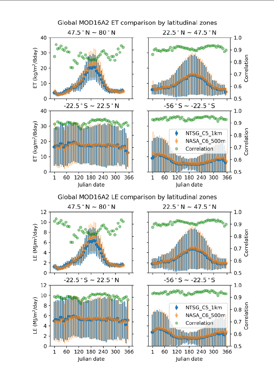
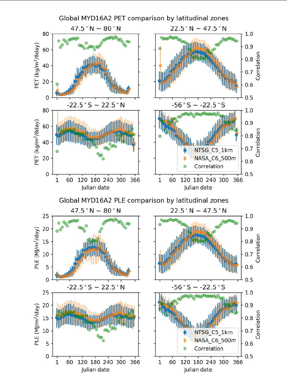
Figure 6.2 shows the seasonality of mean, STD, and correlation for ET, LE, PET and PLE
between baseline NTSG MOD16A2 and NASA operational MOD16A2; and between baseline
NTSG MOD16A2 and NASA operational MYD16A2, respectively. Correspondingly, Table 6.3
shows the averages of difference (
) in mean, relative differences (_
) in %, and average
correlation (
) across all 46 8-days in 2008 between the NASA operational MOD16A2 and
MYD16A2 and NTSG MOD16A2, respectively.
and _
are defined below,
=( )
46
(29)
_
=100
(30)
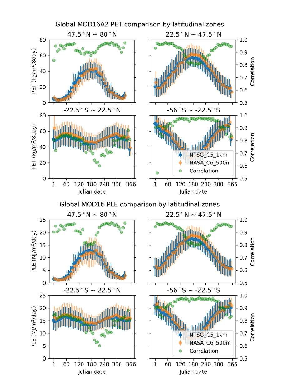
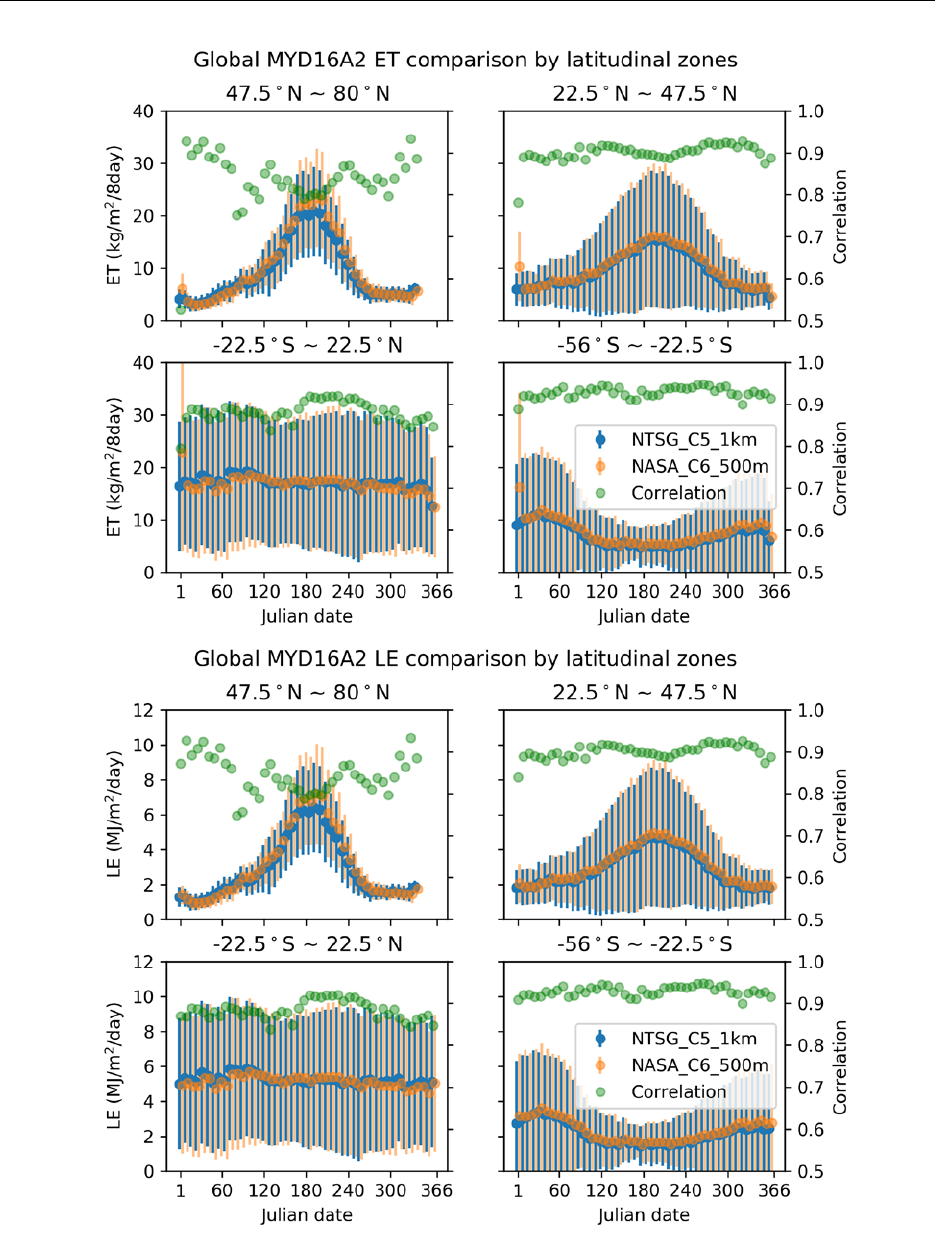
The figures and tables show that both NASA operational C6 MOD16 and MYD16 overall
tend to be higher than NTSG gap-filled MOD16. For ET and LE, the relative differences are
greater in the extra tropics than the tropics, whereas such tendency is opposite for the PET and
PLE. The averages of relative differences for four latitudinal zones are less than 9% and averages
of the correlations are around 0.9, suggesting the closeness of NASA operational MOD16A2 to the
baseline, NTSG gap-filled MOD16A2.
NTSG C5 MOD16A2 has been validated over eddy flux towers (Mu et al., 2011), and the
close agreement in the seasonality between NASA’s operational C5 MOD16A2, MYD16A2 and
NTSG data reveals the reasonability (magnitude, range and directions of variations) of NASA
operational MOD16A2 and MYD16A2 for valid pixels. Based on our evaluations, we conclude
that NASA operational MOD16A2 and MYD16A2 are ready and useful for users to apply the data
to the studies of global terrestrial water and energy cycles and environmental changes.

MOD16 User’s Guide MODIS Land Team
Version 1.6, 08/16/2018 Page 26 of 35
Table 6.3. A) Averages of difference (
), relative differences (_
) in %, and average
correlation (
) across all 46 8-days in 2008 between the NASA operational and NTSG
MOD16A2 by four latitudinal zones.
MOD16A2
ET
LE
PET
PLE
Latitudinal
Zones
,
_
,
_
,
_
,
_
47.5°N~80°N
0.65,
7.06%
0.86
0.20,
6.88%
0.86
-0.57,
-2.73%
0.93
-0.32,
-4.97%
0.92
22.5
°
N~47.5
°
N
0.49,
5.06%
0.91
0.14,
4.76%
0.92
0.90,
2.33%
0.91
0.24,
2.06%
0.91
-22.5
°
S~22.5
°
N
-0.12,
-0.67%
0.90
-0.06,
-1.05%
0.90
2.49,
5.02%
0.77
0.69,
4.55%
0.77
-56°S~-22.5°S
0.56,
7.90%
0.94
0.16,
7.14%
0.934
0.49,
1.00%
0.93
0.05,
0.33%
0.94
Table 6.3. B) Similar to A) but for NASA operational MYD16A2 against NTSG MOD16
MYD16A2
ET
LE
PET
PLE
Latitudinal
Zones
,
_
,
_
,
_
,
_
47.5
°
N~80
°
N
0.66,
7.16%
0.84
0.19,
6.74%
0.84
-0.52,
-2.45%
0.93
-0.32,
-4.83%
0.92
22.5
°
N~47.5
°
N
0.48,
5.08%
0.90
0.12,
4.21%
0.90
1.25,
3.21%
0.91
0.28,
2.33%
0.91
-22.5°S~22.5°N
-0.21,
-1.24%
0.88
-0.11,
-2.11%
0.88
2.88,
5.83%
0.77
0.69,
4.57%
0.78
-56
°
S~-22.5
°
S
0.59,
8.43%
0.93
0.14,
6.62%
0.93
1.00,
2.04%
0.93
0.03,
0.21%
0.94
Authors would like to acknowledge review and feedback from the Land Data Operational
Products Evaluation (LDOPE) at NASA Goddard Space Flight Center and the Land Processes
Distributed Active Archive Center (LP DAAC) at the U.S. Geological Survey (USGS) Earth
Resources Observation and Science (EROS) Center.
MOD16 User’s Guide MODIS Land Team
Version 1.6, 08/16/2018 Page 27 of 35
Figure 6.2. A) The 46 8-day mean, Standard Deviation (STD) of ET and LE for NASA and NTSG
MOD16A2 in year 2008, and the correlation between the two data sets by latitudinal zones.
MOD16 User’s Guide MODIS Land Team
Version 1.6, 08/16/2018 Page 28 of 35
Figure 6.2. B) The 46 8-day mean, Standard Deviation (STD) of PET and PLE for NASA and
NTSG MOD16A2 in year 2008, and the correlation between the two data sets by latitudinal
zones.
MOD16 User’s Guide MODIS Land Team
Version 1.6, 08/16/2018 Page 29 of 35
Figure 6.2. C) The 46 8-day mean, Standard Deviation (STD) of ET and LE for NASA and NTSG
MYD16A2 in year 2008, and the correlation between the two data sets by latitudinal zones.
MOD16 User’s Guide MODIS Land Team
Version 1.6, 08/16/2018 Page 30 of 35
Figure 6.2. D) The 46 8-day mean, Standard Deviation (STD) of PET and PLE for NASA and
NTSG MYD16A2 in year 2008, and the correlation between the two data sets by latitudinal zones.

MOD16 User’s Guide MODIS Land Team
Version 1.6, 08/16/2018 Page 31 of 35
LIST OF NTSG AUTHORED/CO-AUTHORED PAPERS
USING MOD16 ET: 2007 – 2015
[all available at http://www.ntsg.umt.edu/biblio]
Chen, Y., J. Xia, S. Liang, J. Feng, J. B. Fisher, X. Li, X. Li et al. (2014) Comparison of satellite-
based evapotranspiration models over terrestrial ecosystems in China. Remote Sensing of
Environment 140 (2014): 279-293.
Cleugh, H. A., Leuning, R., Mu, Q., and Running, S. W. (2007). Regional evaporation estimates
from flux tower and MODIS satellite data. Remote Sensing of Environment, 106(3), 285-
304.
Jovanovic, N., Mu, Q., Bugan, R. D., and Zhao, M. (2015). Dynamics of MODIS
evapotranspiration in South Africa. Water SA, 41(1), 79-90.
Jung, M., Reichstein, M., Ciais, P., Seneviratne, S. I., Sheffield, J., Goulden, M. L., ... and Dolman,
A. J. (2010). Recent decline in the global land evapotranspiration trend due to limited
moisture supply. Nature, 467(7318), 951-954.
Mu, Q., Heinsch, F. A., Zhao, M., and Running, S. W. (2007). Development of a global
evapotranspiration algorithm based on MODIS and global meteorology data. Remote
Sensing of Environment, 111(4), 519-536.
Mu, Q., Jones, L. A., Kimball, J. S., McDonald, K. C., and Running, S. W. (2009). Satellite
assessment of land surface evapotranspiration for the pan‐Arctic domain. Water Resources
Research, 45(9).
Mu, Q., Zhao, M., and Running, S. W. (2011). Improvements to a MODIS global terrestrial
evapotranspiration algorithm. Remote Sensing of Environment, 115(8), 1781-1800.
Mu, Q., Zhao, M., and Running, S. W. (2011). Evolution of hydrological and carbon cycles under
a changing climate. Hydrological Processes, 25(26), 4093-4102.
Mu, Q., Zhao, M., & Running, S. W. (2012). Remote Sensing and Modeling of Global
Evapotranspiration. In Multiscale Hydrologic Remote Sensing: Perspectives and
Applications (pp. 443-480), edited by Chang, N. B., Hong, Y., CRC Press.
Mu, Q., Zhao M., Kimball J. S., McDowell N., and Running S. W., (2013) A Remotely Sensed
Global Terrestrial Drought Severity Index, Bulletin of the American Meteorological
Society, 94: 83–98.
Renzullo, L. J., Barrett, D. J., Marks, A. S., Hill, M. J., Guerschman, J. P., Mu, Q., and Running,
S. W. (2008). Multi-sensor model-data fusion for estimation of hydrologic and energy flux
parameters. Remote Sensing of Environment, 112(4), 1306-1319.
Ruhoff, A. L., Paz, A. R., Aragao, L. E. O. C., Mu, Q., Malhi, Y., Collischonn, W., ... and Running,
S. W. (2013). Assessment of the MODIS global evapotranspiration algorithm using eddy
covariance measurements and hydrological modelling in the Rio Grande
basin. Hydrological Sciences Journal, 58(8), 1658-1676.
Smettem, K. R., Waring, R. H., Callow, J. N., Wilson, M., and Mu, Q. (2013). Satellite‐derived
estimates of forest leaf area index in southwest Western Australia are not tightly coupled
to interannual variations in rainfall: implications for groundwater decline in a drying
climate. Global Change Biology, 19(8), 2401-2412.
Wang, S., Pan, M., Mu, Q., Shi, X., Mao, J., Brümmer, C., ... and Black, T. A. (2015). Comparing
Evapotranspiration from Eddy Covariance Measurements, Water Budgets, Remote
Sensing, and Land Surface Models over Canada. Journal of Hydrometeorology, 16(4),
1540-1560.

MOD16 User’s Guide MODIS Land Team
Version 1.6, 08/16/2018 Page 32 of 35
Yao, Y., Liang, S., Li, X., Hong, Y., Fisher, J. B., Zhang, N., ... and Jiang, B. (2014). Bayesian
multimodel estimation of global terrestrial latent heat flux from eddy covariance,
meteorological, and satellite observations. Journal of Geophysical Research:
Atmospheres, 119(8), 4521-4545.
Zhang, K., Kimball, J. S., Mu, Q., Jones, L. A., Goetz, S. J., and Running, S. W. (2009). Satellite
based analysis of northern ET trends and associated changes in the regional water balance
from 1983 to 2005. Journal of Hydrology, 379(1), 92-110.

MOD16 User’s Guide MODIS Land Team
Version 1.6, 08/16/2018 Page 33 of 35
REFERENCES
Belward, A. S., Estes, J. E., and Kline, K. D. (1999). The IGBP-DIS global 1-km land-cover data
set DISCover: A project overview. Photogrammetric Engineering and Remote Sensing,
65(9), 1013-1020.
Bouchet, R. J. (1963). Evapotranspiration reelle, evapotranspiration potentielle, et production
agricole. Ann. agron, 14(5), 743-824.
Choudhury, B. J., & DiGirolamo, N. E. (1998). A biophysical process-based estimate of global
land surface evaporation using satellite and ancillary data I. Model description and
comparison with observations. Journal of Hydrology, 205(3-4), 164-185.
Choudhury, B. (2000). A Biophysical Process-Based Estimate of Global Land Surface
Evaporation Using Satellite and Ancillary Data. In Observing Land from Space: Science,
Customers and Technology (pp. 119-126). Springer Netherlands.
Cleugh, H. A., Leuning, R., Mu, Q., and Running, S. W. (2007). Regional evaporation estimates
from flux tower and MODIS satellite data. Remote Sensing of Environment, 106(3), 285-
304.
Courault, D., Seguin, B., and Olioso, A. (2005). Review on estimation of evapotranspiration
from remote sensing data: From empirical to numerical modeling approaches. Irrigation
and Drainage systems, 19(3-4), 223-249.
Dang, Q. L., Margolis, H. A., Coyea, M. R., Sy, M., and Collatz, G. J. (1997). Regulation of
branch-level gas exchange of boreal trees: roles of shoot water potential and vapor pressure
difference. Tree Physiology, 17(8-9), 521-535.
Dawson, T. E., Burgess, S. S., Tu, K. P., Oliveira, R. S., Santiago, L. S., Fisher, J. B., ... and
Ambrose, A. R. (2007). Nighttime transpiration in woody plants from contrasting
ecosystems. Tree Physiology, 27(4), 561-575.
Friedl, M. A., Sulla-Menashe, D., Tan, B., Schneider, A., Ramankutty, N., Sibley, A., and Huang,
X. (2010). MODIS Collection 5 global land cover: Algorithm refinements and
characterization of new datasets. Remote Sensing of Environment, 114(1), 168-182.
Fisher, J. B., Tu, K. P., and Baldocchi, D. D. (2008). Global estimates of the land–atmosphere
water flux based on monthly AVHRR and ISLSCP-II data, validated at 16 FLUXNET
sites. Remote Sensing of Environment, 112(3), 901-919.
Jarvis, P. G. (1976). The interpretation of the variations in leaf water potential and stomatal
conductance found in canopies in the field. Philosophical Transactions of the Royal Society
of London B: Biological Sciences,273(927), 593-610.
Jiang, L., Islam, S., and Carlson, T. N. (2004). Uncertainties in latent heat flux measurement and
estimation: implications for using a simplified approach with remote sensing
data. Canadian Journal of Remote Sensing, 30(5), 769-787.
Jones, H. G. (1992). Plants and microclimate: a quantitative approach to environmental plant
physiology. Cambridge university press.
Kalma, J. D., McVicar, T. R., and McCabe, M. F. (2008). Estimating land surface evaporation: A
review of methods using remotely sensed surface temperature data. Surveys in
Geophysics, 29(4-5), 421-469.
Kawamitsu, Y., Yoda, S., and Agata, W. (1993). Humidity pretreatment affects the responses of
stomata and CO2 assimilation to vapor pressure difference in C3 and C4 plants. Plant and
Cell Physiology, 34(1), 113-119.

MOD16 User’s Guide MODIS Land Team
Version 1.6, 08/16/2018 Page 34 of 35
Kelliher, F. M., Leuning, R., Raupach, M. R., and Schulze, E. D. (1995). Maximum conductances
for evaporation from global vegetation types.Agricultural and Forest Meteorology, 73(1),
1-16.
Leuning, R. (1995). A critical appraisal of a combined stomatal‐photosynthesis model for C3
plants. Plant, Cell & Environment, 18(4), 339-355.
Los, S. O., Pollack, N. H., Parris, M. T., Collatz, G. J., Tucker, C. J., Sellers, P. J., ... and Dazlich,
D. A. (2000). A global 9-yr biophysical land surface dataset from NOAA AVHRR
data. Journal of Hydrometeorology,1(2), 183-199.
Marsden, B. J., Lieffers, V. J., and Zwiazek, J. J. (1996). The effect of humidity on photosynthesis
and water relations of white spruce seedlings during the early establishment
phase. Canadian Journal of Forest Research,26(6), 1015-1021.
Misson, L., Panek, J. A., and Goldstein, A. H. (2004). A comparison of three approaches to
modeling leaf gas exchange in annually drought-stressed ponderosa pine forests. Tree
Physiology, 24(5), 529-541.
Monteith, J. L. (1965). Evaporation and environment. In Symposia of the Society for Experimental
Biology (Vol. 19, p. 205).
Mu, Q., Heinsch, F. A., Zhao, M., and Running, S. W. (2007). Development of a global
evapotranspiration algorithm based on MODIS and global meteorology data. Remote
Sensing of Environment, 111(4), 519-536.
Mu, Q., Zhao, M., and Running, S. W. (2011). Improvements to a MODIS global terrestrial
evapotranspiration algorithm. Remote Sensing of Environment, 115(8), 1781-1800.
Oren, R., Sperry, J. S., Katul, G. G., Pataki, D. E., Ewers, B. E., Phillips, N., and Schäfer, K. V.
R. (1999). Survey and synthesis of intra‐and interspecific variation in stomatal sensitivity
to vapour pressure deficit.Plant, Cell & Environment, 22(12), 1515-1526.
Running, S. W., Loveland, T. R., and Pierce, L. L. (1994). A vegetation classification logic
based on remote sensing for use in global scale biogeochemical models. Ambio, 23, 77-
81.
Running, S. W., Nemani, R. R., Heinsch, F. A., Zhao, M., Reeves, M., and Hashimoto, H. (2004).
A continuous satellite-derived measure of global terrestrial primary
production. Bioscience, 54(6), 547-560.
Running, S. W., and Kimball, J. S. (2005). Satellite‐Based Analysis of Ecological Controls for
Land‐Surface Evaporation Resistance. Encyclopedia of hydrological sciences.
Sandford, A. P., and Jarvis, P. G. (1986). Stomatal responses to humidity in selected conifers. Tree
Physiology, 2(1-2-3), 89-103.
Schubert, S. D., Rood, R. B., and Pfaendtner, J. (1993). An assimilated dataset for earth science
applications. Bulletin of the American meteorological Society, 74(12), 2331-2342.
Schulze, E. D., Kelliher, F. M., Korner, C., Lloyd, J., and Leuning, R. (1994). Relationships among
maximum stomatal conductance, ecosystem surface conductance, carbon assimilation rate,
and plant nitrogen nutrition: a global ecology scaling exercise. Annual Review of Ecology
and Systematics, 629-660.
Shuttleworth, W. J., and Wallace, J. S. (1985). Evaporation from sparse crops‐an energy
combination theory. Quarterly Journal of the Royal Meteorological Society, 111(469),
839-855.
Thornton, P.E. (1998). Regional ecosystem simulation: combining surface- and satellite-based
observations to study linkages between terrestrial energy and mass budgets. PhD.
Dissertation, School of Forestry, The University of Montana, Missoula, MT., 280 pp.

MOD16 User’s Guide MODIS Land Team
Version 1.6, 08/16/2018 Page 35 of 35
Tuzet, A., Perrier, A., and Leuning, R. (2003). Stomatal control of photosynthesis and
transpiration: Results from a soil–plant–atmosphere continuum model. Plant, Cell and
Environment, 26, 1097-1116.
van de Griend, A. A., and Owe, M. (1994). Bare soil surface resistance to evaporation by vapor
diffusion under semiarid conditions. Water Resources Research, 30, 181-188.
Wan, Z., Zhang, Y., Zhang, Q., and Li, Z. L. (2002). Validation of the land-surface temperature
products retrieved from Terra Moderate Resolution Imaging Spectroradiometer
data. Remote sensing of Environment, 83(1), 163-180.
White, M. A., Thornton, P. E., Running, S. W., and Nemani, R. R. (2000). Parameterization and
sensitivity analysis of the BIOME-BGC terrestrial ecosystem model: net primary
production controls. Earth interactions, 4(3), 1-85.
Xu, L., and Baldocchi, D. D. (2003). Seasonal trends in photosynthetic parameters and stomatal
conductance of blue oak (Quercus douglasii) under prolonged summer drought and high
temperature. Tree Physiology, 23(13), 865-877.
Zhao, M., Heinsch, F. A., Nemani, R. R., and Running, S. W. (2005). Improvements of the
MODIS terrestrial gross and net primary production global data set. Remote Sensing of
Environment, 95(2): 164–176.
Zhao, M., Running, S. W., and Nemani, R. R. (2006). Sensitivity of Moderate Resolution
Imaging Spectroradiometer (MODIS) terrestrial primary production to the accuracy of
meteorological reanalyses. Journal of Geophysical Research, 111, G01002,
doi:10.1029/2004JG000004
