Nbody6++ Manual
nbody6%2B%2B_manual
User Manual:
Open the PDF directly: View PDF ![]() .
.
Page Count: 61

NBODY6++
Manual for the Computer Code
Emil Khalisi, Long Wang, Rainer Spurzem
Astronomisches Rechen–Institut
Mönchhofstr. 12–14, 69120 Heidelberg, Germany Kavli Institute for Astronomy and
Astrophysics, Peking University, Beijing, China
Version 4.1
Latest update: September 26, 2018

2

Table of contents 3
Table of contents
1 Introduction..................................... 4
2 Codeversions.................................... 6
3 Gettingstarted.................................... 7
4 Inputvariables.................................... 10
5 Thresholds for the variables . . . . . . . . . . . . . . . . . . . . . . . . . . . . . 21
6 Howtoreadthediagnostics............................. 22
7 Runs on parallel machines . . . . . . . . . . . . . . . . . . . . . . . . . . . . . 27
8 The Hermite integration method . . . . . . . . . . . . . . . . . . . . . . . . . . 28
9 Individual and block time steps . . . . . . . . . . . . . . . . . . . . . . . . . . . 30
10 TheAhmad–Cohenscheme............................. 32
11 KS–Regularization ................................. 35
12 Nbody–units..................................... 37
13 Output........................................ 38
References......................................... 60
4 1 Introduction
1 Introduction
Gravity is an ever–present force in the Universe and is involved into the dynamics of all kinds
of bodies, from the tiny atom to the clusters of galaxies. At small spatial scales, its influence is
covered by other strong forces (e.g. magnetic, pressure, radiation induced), while on the very large
scale it becomes the most dominant power. In astrophysics, it governs the dynamical evolution
of many self–gravitating systems. Here, we concentrate on such systems that are dominated by
mutual gravitation between particles.
The numerical star-by-star simulation of a simple cluster containing some more than hundred
thousand members still places heavy demands on the available hard- and software. A balance has
to be found between two constraints: On one hand the realism, i.e. the input of profound physics,
inclusion of all astrophysical effects as well as the maintenance of the accuracy of calculations;
and on the other hand, the efficiency, i.e. the limitations given by the computational possibilities
and suitable codes to be finished in a reasonable time. Many different kinds of approaches have
been undertaken to suffice both:
•codes based on the direct force integration [2], [5], [6], see also:
,
•statistical models, which themselves divide into several subgroups (Fokker–Planck approx-
imation by [10]; Monte–Carlo method by [13]; Gas models by [27]),
•usage of high-performance parallel computers [28], [11],
•or the construction of special hardware devoted for these purposes (GRAPE [19], see also:
and
∼.
The code NBODY6++ described in this manual is designed for an accurate integration of many
bodies (e.g. in a star cluster, planetary system, galactic nucleus) based on the direct integration
of the Newtonian equations of motion. It is optimal for collisional systems, where long times
of integration and high accuracy or both are required, in order to follow with high precision the
secular evolution of the objects.
NBODY6++ is a descendant of the family of NBODY codes initiated by Sverre Aarseth [4],
which has been extended to be suitable for parallel computers [28]. The basic features of the code
increasing the efficiency may be considered under four separate headings: fourth order prediction–
correction method (Hermite scheme), individual and block time–steps, regularization of close
encounters and few-body subsystems, and a neighbour scheme (Ahmad–Cohen scheme). We
briefly describe these ideas in this booklet, while a detailed description can be found in [3] as well
as his book [6].
While NBODY6++ is not that different from NBODY6 to justify a completely new name, the
user should, however, be aware that in order to make a parallelization of regular and irregular force
computations possible at all, some significant changes in the order of operations became necessary.
As a consequence, trajectories of the same initial system, simulated by NBODY6 and NBODY6++
will diverge from each other, due to the inherent exponential instability and deterministic chaos in
N-body systems. Still one should always expect that the global properties are well behaved in both
cases (e.g. energy conservation). While much effort is taken to keep NBODY6 and NBODY6++
as close as possible this is never 100% the case, and the interested should always contact Sverre
Aarseth or Rainer Spurzem if in doubt about these matters.

5
This manual should serve as a practical starter kit for new students working with NBODY6++.
It is not meant as a complete reference or scientific paper; for that see the references and in
particular the excellent compendium of Aarseth’s book on Gravitational N-Body Simulations [6].
Acknowledgements
The authors of this manual would like to express their sincere gratitude to Sverre Aarseth and
Seppo Mikkola, for their continuous support and work over the decades. Also, many students
and postdocs in Heidelberg and elsewhere have contributed towards development, debugging and
improving the software for the benefit of the community. This booklet was written at the As-
tronomisches Rechen–Institut Heidelberg under the supervision of Rainer Spurzem.
6 2 Code versions
2 Code versions
The development of the NBODY code has begun in the 1960s [1], though there exist some earlier
precursors [29], [30]. It has set a quasi-standard for the precise direct integration of gravitat-
ing many-body systems. There exist several code groups (NBODY0–7, and a number of special
implementations) for different usage, some of which are rather of historical interest.
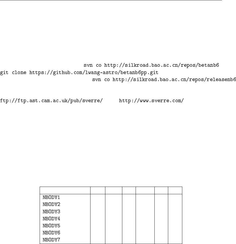
The current NBODY6++ code is available publicly under Subversion or Github. You can
download the beta version by using:
The stable version will be avaiable under
The documents and input samples are included.
The original N–body codes can be accessed publicly via Sverre Aarseth’s ftp and web sites at
and .
A brief comparison of the code versions:
ITS: Individual time–steps
ACS: Neighbour scheme (Ahmad–Cohen scheme) with block time–steps
KS: KS–regularization of few-body subsystems
HITS: Hermite scheme integration method combined with hierarchical block time steps
PN: Post-Newtonian terms
AR: Algorithmic regularization
ITS ACS KS HITS PN AR
X
X X
X X
X X
X X X
X X X
X X X X X
7
3 Getting started
After checkout the NBODY6++ by Subversion or Github (Ch. 2), A directory will be created con-
taining all the source files (routines and functions), documents and input samples. By default the
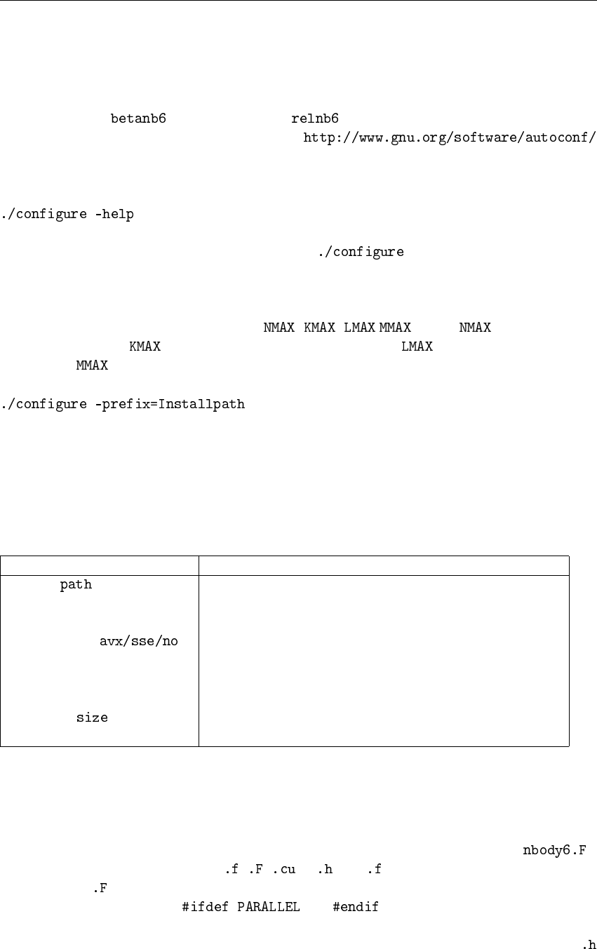
directory is called for beta version and for stable version. The current version use
“configure” scripts generated by GNU Autoconf
to manage the installation. You can check README file for basic examples of using “configure”
to select different features of NBODY6++ for compilation. More details of configure options can
be found by using:
The simple way to use configure is just type: Then the configure script will
check your system environments to find avaiable compilers, make decision for several features like
CUDA, SIMD and HDF5. In this simple example, if all checking pass successfully, there will be
a summary showing the name of excutable file (nbody6++.**), the supported features, installation
path and basic parameters for simulation ( , , , ). Here is the maximum
number of particles, is the maximum number of KS pairs, is the maximum neighbor
number and is the maximum merger number (≥3 bodies stable hierarchical system).
The default installation path is “/user/local”. If you want to change it, use:
Then the code will be installed in “Installpath”.
After successful configure, you just use
make
for compiling the code and
make install
for installation.
The most important options of configure you need to care is shown in Table 3.
Figure 3.0: Options of configure script
Option Description
–prefix= Installation path
–disable-gpu Disable GPU acceleration (In the case you don’t have
Nvidia GPU with cuda support)
–enable-simd= Switch the features of SIMD parallel method (AVX / SSE
/ NONE)
–disable-mpi Disable MPI parallelization
–disable-openmp Disable OpenMP support
–with-par= Choose the simulation parameters (NMAX, KMAX,
LMAX, MMAX), see detail by “./configure –help”
The document file is saved in “Installpath/share/doc”. The input samples are in directory
samples in your code directory.
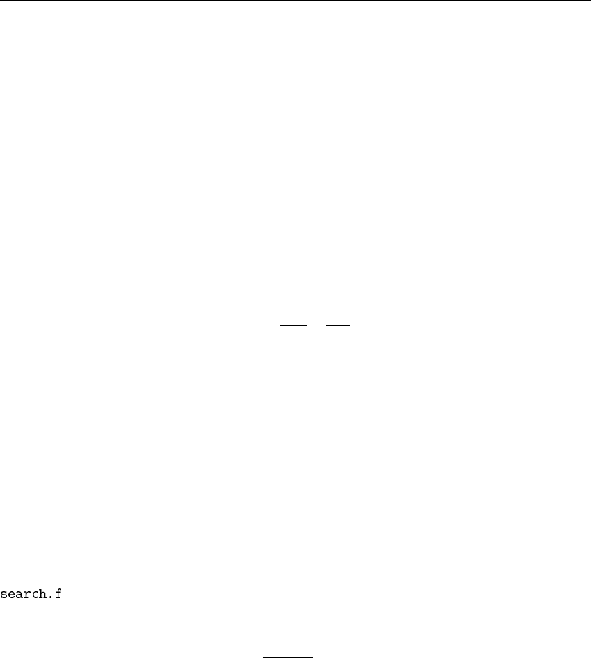
The code NBODY6++ is written in Fortran 77 and consists of about 300 files. Their function-
ality was improved as well as new routines included all the way through the decades along with
the technological achievements of the hardware. The starting (main) routine is called .
Most of the files have the suffix , , or . All files are directly read by a Fortran
compiler. The files will pass preprocessor first, which selects code lines separated by prepro-
cessor options, e.g. between and , for they activate the parallel code
on different multiprocessor machines. By this, some portability between different hardware is en-
sured at least, and a single processor version of the code can easily be compiled as well. The
8 3 Getting started
are header files and declare the variables and their blocks.
Depending on the user’s individual research, the Nbody code opens a wide field of application
possibilities. The user has to define his model by a number of input control variables, e.g. number
of stars, the size of the cluster, a mass function, profile, and many more. These control variables
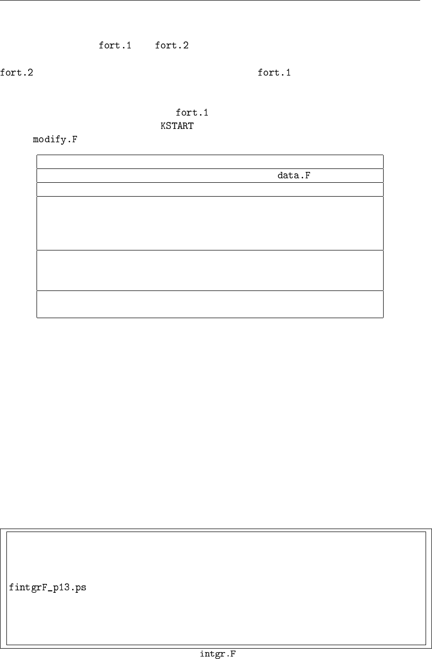
are gathered in the input files. The detailed explanation of its handling is given in Chapter 4. Al-
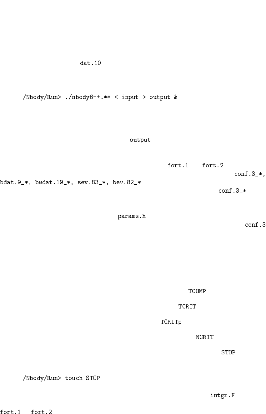
ternatively, a data file named can be used, which contains data for an initial configuration
(see Ch. 4). If the model criteria are defined, a single processor simulation run is started with the
command
homedir
In this example, the code reads the control variables given in the input file from Unix standard
input stdin. Then, a star cluster is created according to the user’s instructions, and the bodies are
moved one by one with respect to their time maturity. Some first results and error checks are
directed via the Unix standard output stdout to . This file provides snapshots of the state
of the system for a brief overview of some key data of the simulation to judge about the quality
and performance of the run.
There are several more files created. Most important are and , which contain
dumps of the complete common blocks for a restart and checkpoint purposes, and
that contain the particle data for the user’s
analysis. The detail descriptions of output files are shown in Ch. 13. In the , many
details of the run are saved, e.g. positions, velocities, neighbour densities, potential of each par-
ticle in any predefined time interval. The volume of data in all three mentioned files critically
depends on the dimensions of vectors in . Here, the particle data plus some user-
defined dimensions are given a threshold in order to save disk space when outputting to
— see Chapter 5.
At the time of this writing, the user has to provide own routines to postprocess the particle data
from the simulation, using e.g. additional routines or programs (like IDL, gnuplot etc.), in order
to extract the binary data from this file and plot graphics. Work is in progress to provide a better
visual interface delivered with the program.
A run will be finished when one of 4 conditions becomes true:
•the specified CPU–time on the computer is exceeded (variable in the input file), or
•the maximum Nbody–time (see Ch. 4) is reached (variable ), or
•the physical cluster time in Myr is reached (variable ), or
•the number of cluster stars has fallen below a minimum (variable ).
A soft termination of a running simulation can be realized by generating of a file in the exe-
cuting directory:
homedir
In that case, a checkpoint of the code is done, which is located in the routine and shown
in Figure 3.1. The program writes out the current variables, saves a complete common dump in
or and terminates. The run can be restarted and continued from the same point
where it was left.
9
Before a restart, it is recommendable to copy or rename the files, otherwise they may be
overwritten. Any file and is restartable. The different names are just for get-
ting common dumps at different time units. For example, if an irregular termination takes place,
contains the data at some earlier time point, while always contains the last time
data.
To restart a run, a different very short input control data file needs to be used, because most
of the control data are already stored in . Only the first line corresponds to the standard
input file, but the first input variable, , has to be changed to “2” or higher. In this case, the
routine will be entered.
KSTART Function
1 new run, start from initial values given in
2 continuation of a run without changes
3 restart of a run with changes of the following parameters given in
the second line of a newly created input file:
DTADJ, DELTAT, TADJ, TNEXT, TCRIT, QE, J, K
where the options KZ can be changed via KZ(J)=K
4 restart of a run with following parameters changed in the second
line: ETAI, ETAR, ETAU, DTMIN, RMIN, NCRIT, NNBOPT,
SMAX
5 restart of a run with all parameter changes in the run control index
3 and 4. The changes must succeed the first line.
“0” values in the fields are interpreted as: Do not change the value of this parameter.
The details of input and restart are discussed in Ch. 4.
Figure 3.1: Soft interruption of a simulation run in : If the dummy file “STOP” exists, then the run
terminates.
10 4 Input variables
4 Input variables
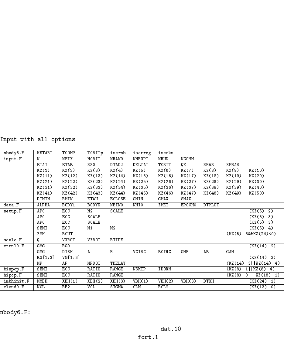
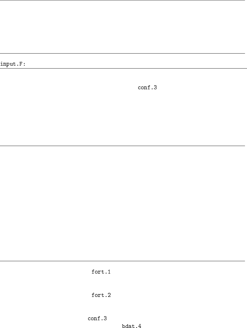
The input control file of NBODY6++ (see below), contains a minimum of 90 parameters which
guide one simulation run for its technical and physical properties (it is very similar but not identical
to the one used for NBODY6). As for the technical aspect, the file supervises the run e.g. for its
duration, intervals of the output, or error check; the physical parameters concern the size of a
cluster, initial conditions, or a number of optional features related to the numerical problem to be
studied. The handling of this input file appears rather entangled at first sight, for it has grown
rather historically and “ready–for–use” than custom–oriented. Thus, the input variables are read
by different routines (functions) in the code, and the nature of the parameters are woven with each
other in some cases. Also, some parameters require additional input, such that the total number of
lines and parameters may vary.
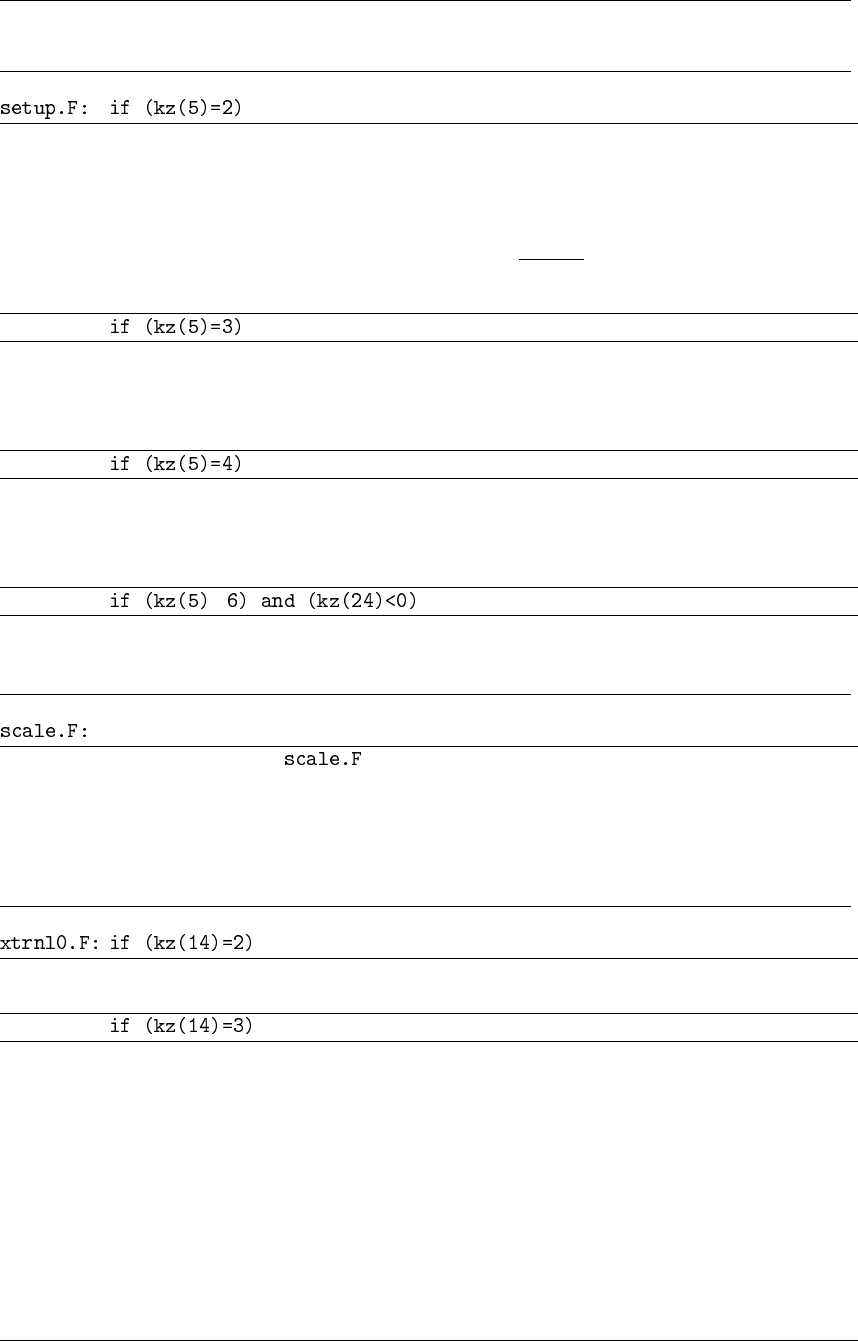
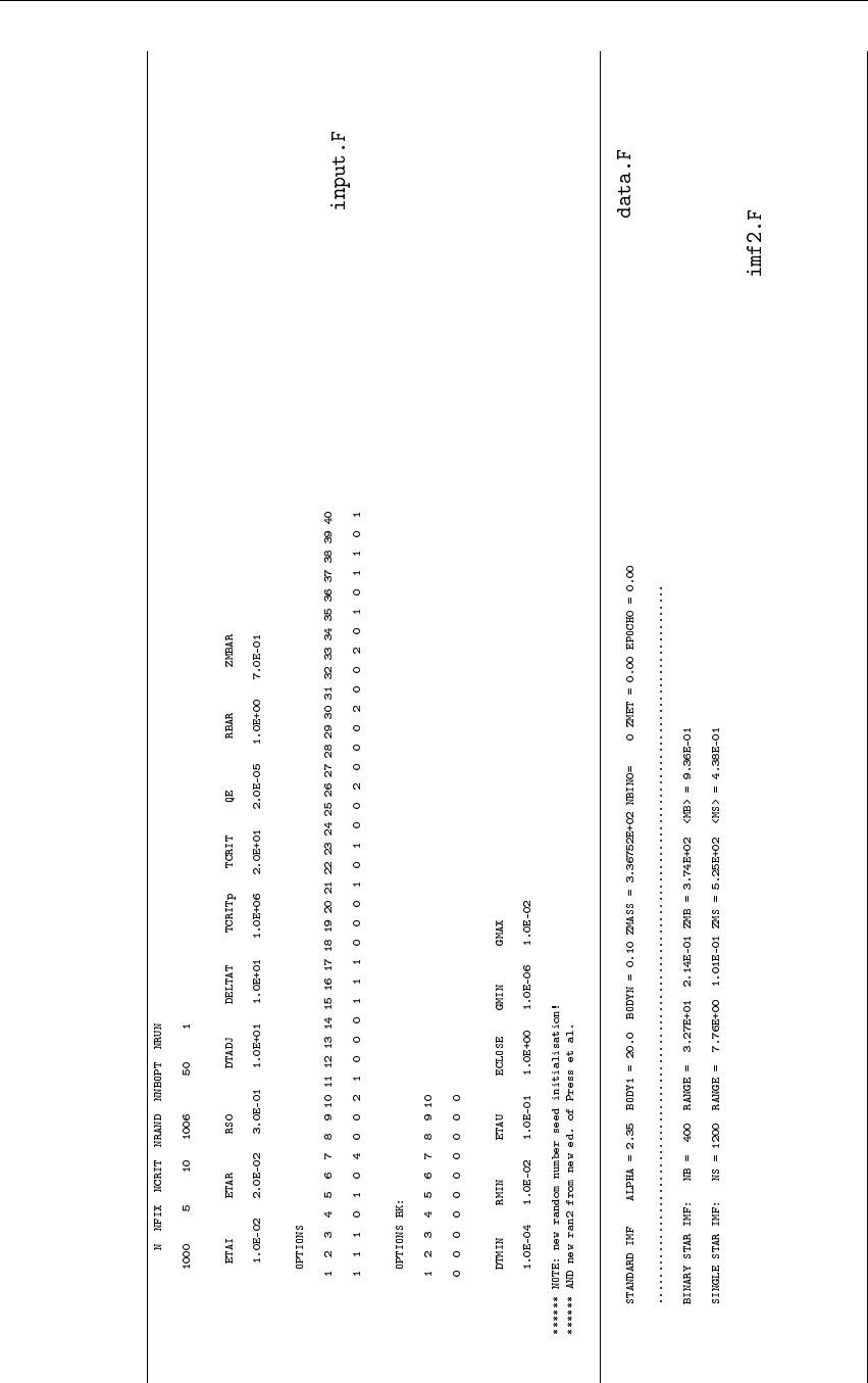
In the following, we explain the main input file and give an example of typical values for a
simulation of an isolated globular cluster. Then, we proceed to the thresholds.
:
=
=
=
=
=
=
=
= =
=>
>&& >
=
>
KSTART Run control index
=1: new run (construct new model or read from )
=2: restart/continuation of a run, needs
=3: restart + changes of DTADJ, DELTAT, TADJ, TNEXT, TCRIT, QE, J, KZ(J)
=4: restart + changes of ETAI, ETAR, ETAU, DTMIN, RMIN, NCRIT, NNBOPT,
SMAX
=5: restart containing the combination of the control index 3 and 4
TCOMP Maximum wall-clock time in seconds (parallel runs: wall clock)
TCRITP Termination time in Myr
isernb For MPI parallel runs: only irregular block sizes larger than this value are executed
in parallel mode (dummy variable for single CPU)
11
iserreg For MPI parallel runs: only regular block sizes larger than this value are executed in
parallel mode (dummy variable for single CPU)
iserks For MPI parallel runs: only ks block sizes larger than this value are executed in
parallel mode (dummy variable for single CPU)
N Total number of particles (single + c.m.s. of binaries; singles + 3×c.m.s. of binaries
< NMAX−2)
NFIX Multiplicator for output interval of data on and of data for binary stars (output
each DELTAT×NFIX time steps; compare KZ(3) and KZ(6))
NCRIT Minimum particle number (alternative termination criterion)
NRAND Random number seed; any positive integer
NNBOPT Desired optimal neighbour number (< LMAX−5)
NRUN Run identification index
NCOMM Frequency to store the dumping data (mydump)
ETAI Time–step factor for irregular force polynomial
ETAR Time–step factor for regular force polynomial
RS0 Initial guess for all radii of neighbour spheres (N–body units)
DTADJ Time interval for parameter adjustment and energy check (N–body units)
DELTAT Time interval for writing output data and diagnostics, multiplied by NFIX (N–body
units)
TCRIT Termination time (N–body units)
QE Energy tolerance:
– immediate termination if DE/E > 5*QE & KZ(2) ≤1;
– restart if DE/E > 5*QE & KZ(2) > 1 and termination after second restart attempt.
RBAR Scaling unit in pc for distance (N–body units)
ZMBAR Scaling unit for average particle mass in solar masses
(in scale-free simulations RBAR and ZMBAR can be set to zero; depends on KZ(20))
KZ(1) Save COMMON to file
=1: at end of run or when dummy file STOP is created
=2: every 100*NMAX steps
KZ(2) Save COMMON to file
=1: save at output time
=2: save at output time and restart simulation if energy error DE/E > 5*QE
KZ(3) Save basic data to file at output time (unformatted)
KZ(4) (Suppressed) Binary diagnostics on (# = threshold levels <10)
KZ(5) Initial conditions of the particle distribution, needs KZ(22)=0
=0: uniform & isotropic sphere
=1: Plummer random generation
=2: two Plummer models in orbit (extra input)
=3: massive perturber and planetesimal disk (each pariticle has circular orbit, con-
stant separation along radial direction between each neighbor and random phase)
(extra input)
=4: massive initial binary (extra input)
12 4 Input variables
=5: Jaffe model (extra input)
≥6: Zhao BH cusp model (extra input if KZ(24)<0)
KZ(6) Output of significant and regularized binaries at main output ( )
=1: output regularized and significant binaries (|E|>0.1 ECLOSE)
=2: output regularized binaries only
=3: output significant binaries at output time and regularized binaries with time
interval DELTAT
=4: output of regularized binaries only at output time
KZ(7) Determine Lagrangian radii and average mass, particle counters, average velocity,
velocity dispersion, rotational velocity within Lagrangian radii ( )
=1: Get actual value of half mass radius RSCALE by using current total mass
≥2: Output data at main output and
≥6: Output Lagrangian radii for two mass groups at and
( ; based on KZ(5)=1,2; cost is O(N2))
—- methods:
=2,4: Lagrangian radii calculated by initial total mass
=3,≥5: Lagrangian radii calculated by current total mass (The single/K.S-binary
Lagrangian radii are still calculated by initial single/binary total mass)
=2,3: All parameters are averaged within the shell between two Lagrangian radii
neighbors
≥4: All parameters are averaged from center to each Lagrangian radius
KZ(8) Primordial binaries initialization and output ( )
—- Initialization:
=0: No primordial binaries
=1,≥3: generate primordial binaries based on KZ(41) and KZ(42) ( )
=2: Input primordial binaries from first 2×NBIN0 lines of
—- Output:
>0: Save information of primordial binary that change member in ; binary
diagnostics at main output ( )
≥2: Output KS binary in , soft binary in at output time
KZ(9) Binary diagnostics
=1,3: Output diagnostics for the hardest binary below ECLOSE in
( )
≥2: Output binary evolution stages in ( )
≥3: Output binary with degenerate stars in ( )
KZ(10) K.S. regularization diagnostics at main output
>0: Output new K.S. information
>1: Output end K.S. information
≥3: Output each integrating step information
KZ(11) (Suppressed)
KZ(12) >0: HR diagnostics of evolving stars with output time interval DTPLOT in
(single star) and (K.S. binary)
=−1: used if KZ(19)=0 (see details in KZ(19) description)
KZ(13) Interstellar clouds
=1: constant velocity for new cloud
>2: Gaussian velocity for new cloud
KZ(14) External tidal force
=1: standard solar neighbor tidal field
13
=2: point-mass galaxy with circular orbit (extra input)
=3: point-mass + disk + halo + Plummer (extra input)
=4: Plummer model (extra input)
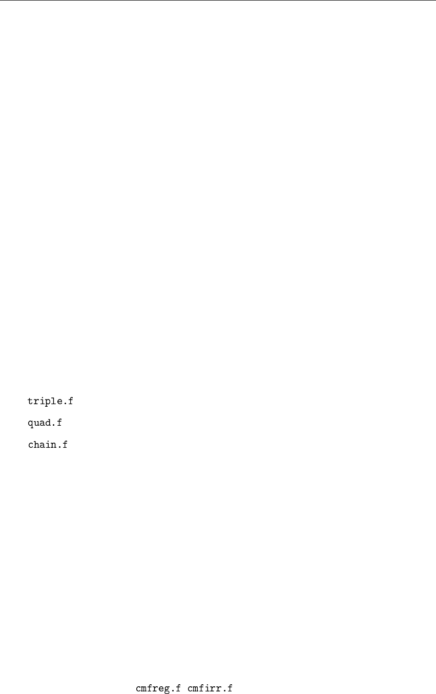
KZ(15) Triple, quad, chain and merger search
≥1: Switch on triple, quad, chain (KZ(30)>0) and merger search ( )
≥2: Diagnostics at main output at begin and end of triple, quad
≥3: Save first five outer orbits every half period of wide quadruple before merger
and stable quadruples accepted for merger in
KZ(16) Auto-adjustment of regularization parameters
≥1: Adjust RMIN, DTMIN & ECLOSE every DTADJ time
≥3: modify RMIN for GPERT > 0.05 or < 0.002 in chain; output diagnostics at
KZ(17) Auto-adjustment of ETAI, ETAR and ETAU by tolerance QE every DTADJ time
( )
≥1: Adjust ETAI, ETAR
≥2: Adjust ETAU
KZ(18) Hierarchical systems
=1,3: diagnostics ( )
≥2: Initialize primordial stable triples, number is NHI0 ( )
≥4: Data bank of stable triple, quad in ( )
KZ(19) Stellar evolution mass loss
=0: if KZ(12)=−1, the output data will keep the input data unit if KZ(22)=2−4
or N-body units if KZ(22)=6−10
=1,2: supernova scheme
≥3: Eggleton, Tout & Hurley
≥5: extra diagnostics (mdot.F)
=2,4: Input stellar parameters from ( )
N lines of (MI, KW, M0, EPOCH1, OSPIN)
MI: Current mass
KW: Kstar type
M0: Initial mass
EPOCH1: evolved age of star (Age =TIME[Myr] −EPOCH1)
OSPIN: angular velocity of star
KZ(20) Initial mass functions, need KZ(22)=0 or 9:
=0: self-defined power-law mass function using ALPHAS ( )
=1: Miller-Scalo-(1979) IMF ( )
=2,4: KTG (1993) IMF ( )
=3,5: Eggleton-IMF ( )
=6,7: Kroupa(2001) ( ), extended to Brown Dwarf regime ( )
—- Primordial binary mass
=2,6: random pairing ( )
=3,4,5,7: binary mass ratio corrected by (m1/m2)0= (m1/m2)0.4+ constant (Eggle-
ton, )
=8: binary mass ratio q=m1/m2(m2≤m1) use distribtution 0.6q−0.4(Kouwen-
hoven)
KZ(21) Extra diagnostics information at main output every DELTAT interval ( )
≥1: output NRUN, MODEL, TCOMP, TRC, DMIN, AMIN, RMAX, RSMIN,
NEFF
14 4 Input variables
≥2: Number of escapers NESC at main output will be counted by Jacobi escape
criterion (cost is O(N2), )
KZ(22) Initialization of basic particle data mass, position and velocity ( )
—- Initialization with internal method
=0,1: Initial position, velocity based on KZ(5), initial mass based on KZ(20)
=1: write initial conditions in ( )
—- Initialization by reading data from
=2: input through NBODY-format (7 parameters each line: mass, position(1:3),
velocity(1:3))
=3: input through Tree-format ( )
=4: input through Starlab-format
=6: input through NBODY-format and do scaling
=7: input through Tree-Format and do scaling
=8: input through Starlab-format and do Scaling
=9: input through NBODY-format but ignore mass (first column) and use IMF based
on KZ(20), then do scaling
=10: input through NBODY-format and all units are astrophysical units (mass: M;
position: pc; velocity: km/s)
KZ(23) Removal of escapers ( )
≥1: remove escapers and ghost particles generated by two star coalescence (colli-
sion)
=2,4: write escaper diagnostics in
≥3: initialization & integration of tidal tail
KZ(24) Initial conditions for subsystems
<0: ZMH & RCUT (N-body units) Zhao model (Need KZ(5)≥6, )
=1: Add one massive black hole (extra input: mass, position, velocity and output
frequency), will output black hole data in and its neighbor data in
KZ(25) Velocity kicks for white dwarfs ( )
=1: Type 10 Helium white dwarf & 11 Carbon-Oxygen white dwarf
=2: All WDs (type 10, 11 and type 12 Oxygen-Neon white dwarf)
KZ(26) Slow-down of two-body motion, increase the regularization integration efficiency
≥1: Apply to KS binary
≥2: Apply to chain
=3: Rectify to get better energy conservation
KZ(27) Two-body tidal circularization (Mardling & Aarseth, 2001; Portegies Zwart et al.
1997)
(Please suppress in KS parallel version)
=1: sequential
=2: chaos
=3: GR energy loss
=−1: Only detect collision and suppress coalescence
KZ(28) Magnetic braking and gravitational radiation for NS or BH binaries (Need KZ(19)=3
and based on KZ(27))
≥1: GR coalescence for NS & BH ( , )
≥2: Diagnostics at main output ( )
=3: Input of ZMH = 1/SQRT(2*N) (Need KZ(5)≥6) ( )
=4: Set every star as type 13 Neutron star (Need KZ(27)=3) ( )
KZ(29) (Suppressed) Boundary reflection for hot system
15
KZ(30) Hierarchical system regularization
=−1: Use chain only
=0: No triple, quad and chain regularization, only merger
=1: Use triple, quad and chain ( )
≥2: Diagnostics at begin/end of chain at main output
≥3: Diagnostics at each step of chain at main output
KZ(31) Centre of mass correction after energy check ( )
KZ(32) Adjustment (increase) of adjust interval DTADJ, output interval DELTAT and energy
error criterion QE based on binding eneryg of cluster ( )
KZ(33) Block-step statistics at main output (diagnostics)
≥1: Output irregular block step; and K.S. binary step if KZ(8)>0
≥2: Output regular block step
KZ(34) Roche-lobe overflow
=1: Roche & Spin synchronisation on binary with circular orbit ( )
=2: Roche & Tidal synchronisation on binary with circular orbit by BSE method
( )
KZ(35) TIME reset to zero every 100 time units, total time is TTOT = TIME + TOFF
( )
KZ(36) (Suppressed) Step reduction for hierarchical systems
KZ(37) Neighbour list additions ( )
≥1: Add high-velocity particles into neighbor list
≥2: Add small time step particle (like close encounter particles near neighbor radius)
into neighbor list
KZ(38) Force polynomial corrections during regular block step calculation
=0: no corrections
=1: all gains & losses included
=2: small regular force change skipped
=3: fast neighbour loss only
KZ(39) Neighbor radius adjustment method
=0: The system has unique density centre and smooth density profile
=1,≥3: The system has no unique density centre or smooth density profile
skip velocity modification of RS(I) ( , )
do not reduce neighbor radius if particle is outside half mass radius
reduce RS(I) by multiply 0.9 instead of estimation of RS(I) based on
NNBOPT/NNB when neighbor list overflow happens ( , )
=2,3: Consider sqrt(particle mass / average mass) as the factor to determine the
particle’s neighbor membership. ( , )
KZ(40) =0: For the initialization of particle time steps, use only force and its first derivative
to estimate. This is very efficent.
>0: Use Fploy2 (second and third order force derivatives calculation) to estimate the
initial time steps. This method provide more accurate time steps and avoid incorrent
time steps for some special cases like initially cold systems, but the computing cost
is much higher (O(N2))
KZ(41) proto-star evolution of eccentricity and period for primordial binaries initialization
( , )
KZ(42) Initial binary distribution
=0: RANGE>0: uniform distribution in log(semi) between SEMI0 and
SEMI0/RANGE
16 4 Input variables
RANGE<0: uniform distribution in semi between SEMI0 and -1*RANGE.
=1: linearly increasing distribution function f=0.03438 ∗logP
=2: f=3.5logP/[100 + (logP)∗∗2]
=3: f=2.3(logP −1)/[45 + (logP −1)∗∗2]; This is a “3rd” iteration when pre-ms
evolution is taken into account with KZ(41)=1
=4: f=2.5(logP−1)/[45+(logP−1)∗∗2]; This is a “34th” iteration when pre-ms
evolution is taken into account with KZ(41)=1 and RBAR<1.5
=5: Duquennoy & Mayor 1991, Gaussian distribution with mean logP=4.8, SDEV
in logP=2.3. Use Num.Recipes routine to obtain random deviates given
“idum1”
KZ(43) (Unused)
KZ(44) (Unused)
KZ(45) (Unused)
KZ(46) HDF5/BINARY/ANSI format output and global parameter output (main output, see
chapter 13 for details)
=1,3: HDF5(if HDF5 is compiled)/BINARY format
=2,4: ANSI format
=1,2: Only output active stars with time interval defined by KZ(47)
=3,4: Output full particle list with time interval defined by KZ(47)
KZ(47) Frequency for KZ(46) output
Output data with time interval 0.5KZ(47)×SMAX
KZ(48) (Unused)
KZ(49) Computation of Moments of Inertia (with Chr. Theis) in ( )
KZ(50) For unperted KS binary. The neighbor list is searched for finding next KS step. It is
safer to get correct step but not efficient when unperted binary number is large. To
suppress this, set to 1
DTMIN Time–step criterion for regularization search
RMIN Distance criterion for regularization search
ETAU Regularized time-step parameter (6.28/ETAU steps/orbit)
ECLOSE Binding energy per unit mass for hard binary (positive)
GMIN Relative two-body perturbation for unperturbed motion
GMAX Secondary termination parameter for soft KS binaries
SMAX Maximum time-step (factor of 2 commensurate with 1.0)
ALPHA Power-law index for initial mass function, routine
BODY1 Maximum particle mass before scaling (based on KZ(20); solar mass unit)
BODYN Minimum particle mass before scaling
NBIN0 Number of primordial binaries (need KZ(8)>0)
– by routine using a binary IMF (KZ(20)≥2)
– by routine splitting single stars (KZ(8)>0)
– by reading subsystems from (KZ(22)≥2)
NHI0 Number of primordial hierarchical systems (need KZ(18)≥2)
ZMET Metal abundance (in range 0.03 - 0.0001)
EPOCH0 Evolutionary epoch (in 106yrs)
DTPLOT Plotting interval for stellar evolution HRDIAG (N-body units; ≥DELTAT)
17
APO Separation of two Plummer models in N–body units (SEMI = APO/(1 +ECC). (No-
tice SEMI will be limited between 2.0 and 50.0)
ECC Eccentricity of two-body orbit (ECC ≥0 and ECC < 0.999)
N2 Membership of second Plummer model (N2 <= N)
SCALE Scale factor for the second Plummer model, second cluster will be generated by first
Plummer model with X×SCALE and V×√SCALE(≥0.2 for limiting minimum
size)
APO Separation between the perturber and Sun in N–body units
ECC Eccentricity of orbit (=1 for parabolic encounter)
SCALE Perturber mass scale factor, perturber mass = Center star mass ×SCALE (=1 for
Msun)
SEMI Semi-major axis (slightly modified; ignore if ECC > 1)
ECC Eccentricity (ECC > 1: NAME = 1 & 2 free-floating)
M1 Mass of first member (in units of mean mass)
M2 Mass of second member (rescaled total mass = 1)
≥
ZMH Mass of single BH (in N-body units)
RCUT Radial cutoff in Zhao cusp distribution (MNRAS, 278, 488)
Q Virial ratio (routine ; Q=0.5 for equilibrium)
VXROT XY–velocity scaling factor (> 0 for solid-body rotation)
VZROT Z–velocity scaling factor (not used if VXROT = 0)
RTIDE Unscaled tidal radius for KZ(14)=2 and KZ(22)≥2. If not zero, RBAR = RT/RTIDE
where RT[pc] is tidal radius calculated from input GMG and RG0
GMG Point-mass galaxy (solar masses, linearized tidel field in circular orbit)
RG0 Central distance (in kpc)
GMG Point-mass galaxy (solar masses)
DISK Mass of Miyamoto disk (solar masses)
A Softening length in Miyamoto potential (in kpc)
B Vertical softening length (kpc)
VCIRC Galactic circular velocity (km/sec) at RCIRC (=0: no halo)
RCIRC Central distance for VCIRC with logarithmic potential (kpc)
GMB Dehnen model budge mass (solar masses)
AR Dehnen model budge scaling radius (kpc)
GAM Dehnen model budge profile power index gamma
RG Initial position; DISK+VCIRC=0, VG(3)=0: A(1+E)=RG(1), E=RG(2)
VG Initial cluster velocity vector (km/sec)
18 4 Input variables
MP Total mass of Plummer sphere (in scaled units)
AP Plummer scale factor (N-body units; square saved in AP2)
MPDOT Decay time for gas expulsion (MP = MP0/(1 + MPDOT*(T-TD))
TDELAY Delay time for starting gas expulsion (T > TDELAY)
SEMI Initial semi-major axis limit
ECC Initial eccentricity
<0: thermal distribution, f(e) = 2e
≥0 and ≤1: fixed value of eccentricity
=20: uniform distribution
=30: distribution with f(e) = 0.1765/(e2)
=40: general f(e) = a∗eb,e0<=e<=1 with a= (1+b)/(1−e0(1+b)), current
values: e0=0 and b=1 (thermal distribution)
RATIO KZ(42)≤1: Binary mass ratio M1/(M1+M2)
KZ(42)=1.0: M1=M2=hMi
RANGE KZ(42)=0: semi-major axis range for uniform logarithmic distribution;
not used for other KZ(42)
NSKIP Binary frequency of mass spectrum (starting from body #1)
IDORM Indicator for dormant binaries (>0: merged components)
SEMI Max semi-major axis in model units (all equal if RANGE = 0)
ECC Initial eccentricity (<0 for thermal distribution)
RATIO Mass ratio (=1.0: M1=M2; random in [0.5∼0.9])
RANGE Range in SEMI for uniform logarithmic distribution (>0)
MMBH Mass of massive black hole in solar mass unit
XBH(1:3) 3 dimensional position of massive black hole in pc
VBH(1:3) 3 dimensional velocity of massive black hole in km/s
DTBH Output interval for massive black hole data in and (N-body unit)
NCL Number of interstellar clouds
RB2 Radius of cloud boundary in pc (square is saved)
VCL Mean cloud velocity in km/sec
SIGMA Velocity dispersion (KZ(13)>1: Gaussian)
CLM Individual cloud masses in solar masses (maximum MCL)
RCL2 Half-mass radii of clouds in pc (square is saved)
19
A typical input file can look like as follows. It defines a new simulation running for 1,000,000
CPU–minutes with N=16,000 particles distributed from a Plummer profile (KZ(5)=1). The run
may alternatively terminate when TCRIT=1000.0 N–body units. or if the final particle number of
NCRIT=10 has been reached. The output and adjustment time interval DELTAT/DTADJ are 1.0
N-body unit. The initial mass function follows Kroupa, (2001) with mass ranging from mmax =
20.0Mto mmin =0.08M(BODY1 and BODYN). The initial virial ratio is 0.5 (equilibrium).
The stellar evolution is switched on (KZ(19)=3) and initial metallicity is 0.001. Multiples and
chain regularization are switched on (KZ(15)=2 and KZ(30)=2). It uses solar neighbor tidal field
(KZ(14)=1).
Input variables for primordial Binaries
Many star clusters contain initial hard binaries with binding energies much larger than the thermal
energy (the threshold ECLOSE is a suitable division between hard and soft binaries). There are
two ways to initialise primordial binaries:
The first one always starts from some initial mass function (IMF) provided by the routines
or . The option KZ(8)=1 or ≥3 invokes the routine , which reads the last
line of the input file containing NBIN and the parameters of their distribution (see above). In this
case, binaries are created either by random pairing of single stars obtained from the IMF or by
splitting them, depending on the value of KZ(20) (see above).
The second way assumes that particle data, including the binaries, are provided via the input
data on file (as e.g. in the Kyoto–II collaborative experiment). In such a case KZ(8)=2
and NBIN0 should be set to the expected number of primordial binaries from the file. The code
will first create NBIN0 centers of masses, and then use those for scaling, before regularizing the
pairs and the calculation begins.
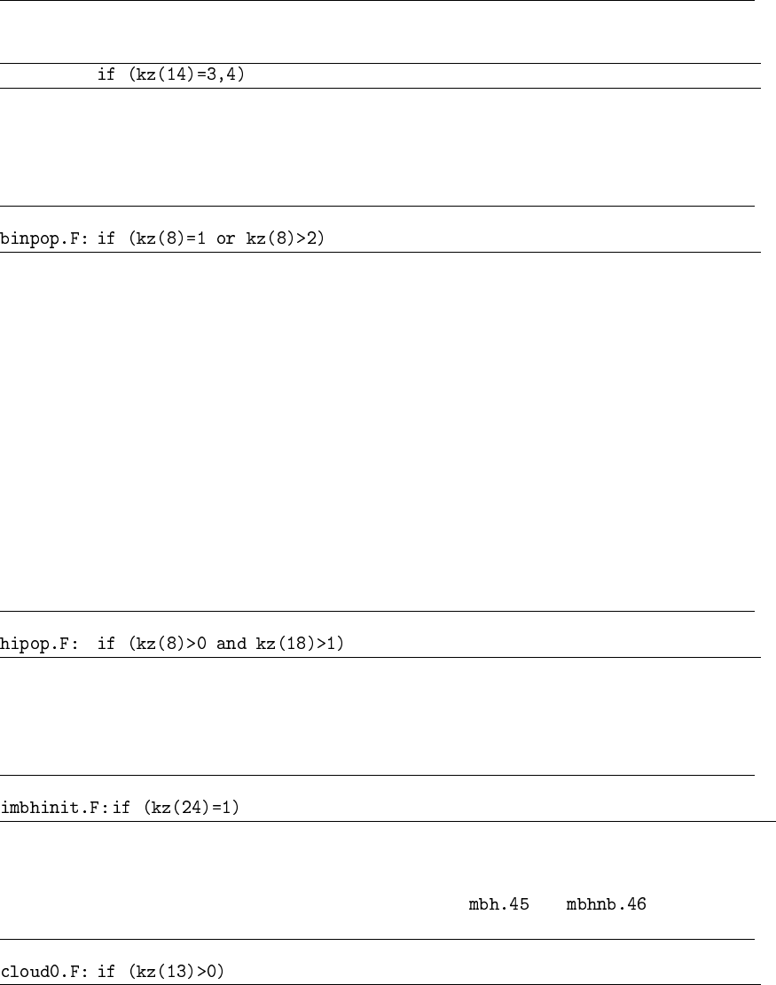
A typical input file with primordial binaries looks as follows. Here, we use binary random pair-
ing from and (KZ(20)=6 and KZ(8)=3, respectively) for 1000 initial binaries.
The semi-major axes of binaries use uniform distribution in log(semi) with a range from 41.3 AU
to 0.00413 AU. The eccentricity of binaries use thermal distribution. It was created from this input
file running for 1000 time units. Stellar evolution was also switched on in this file (KZ(19)=3). In
the package of the code, the file is included.
20 4 Input variables
Stellar Evolution
Stellar evolution is invoked by KZ(19)=1,2 or KZ(19)≥3, offering two different schemes. The
simpler one is KZ(19)=1, while the more complex one, K(19)≥3, is based on the Cambridge
stellar evolution package (Hurley, Pols, Tout 2000). The common envelope, roche transfering
binaries are also considered. The main effects are changing stellar masses, radii, and luminosities,
which give rise to cluster mass loss. The mass is assumed to escape from the cluster immediately
and possible collisions depend on stellar radii.
With the additional option KZ(12)>0, information on binaries and single stars is written on
two files (unit 82, file and unit 83, file ) in regular time intervals determined by
TPLOT (See details in Section Output).
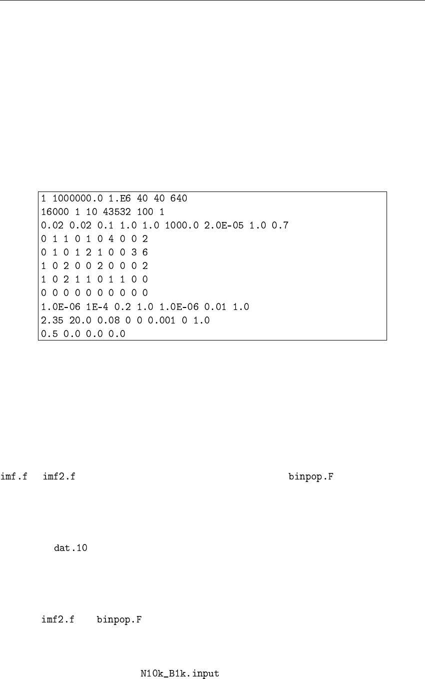
Restart
It’s very common that in the computer cluster every job has running time limit, or the simula-
tion stop due to some energy conservation problem or the normal stop when the stop criterion is
reached. In this case the user may want to continue the simulation from the last time point. Thus
the input parameter should changed to restart mode. The first line of input shown above combined
together with two extra lines (See the description of KSTART in the parameter table above). A
simple example is :
Here KSTART=2 means every parameter keeps the same value as before and just restarts
from the last saved file . If the user wants to change some parameters of simulation,
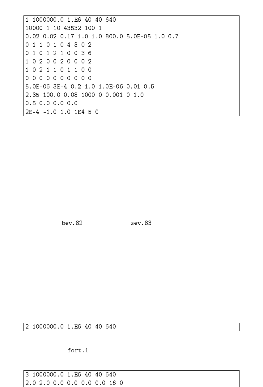
KSTART=3,5 can be set. For example:
This restart file will change DTADJ and DELTAT to 2.0. The KZ(16) is changed to 0. All
other parameters that are set to 0.0 (TADJ, TNEXT, TCRIT, QE) keep same as before.
21
5 Thresholds for the variables
Before the compilation of the code (Chapter 3), the parameter file ( ) should be consulted
to check whether some vector dimensions are in the desired range. Most important are
•the maximum particle number ,
•the maximum number of regularised KS pairs , and
•the maximum number of neighbours per particle .
The particles are saved in various lists which serve to distinguish between their funcionality.
The table below explains their nomenclature. “KS–pairs” are particles that approach each other
in a hyperbolic encounter; they are given a special treatment by the code (see Chapter 11). If
NPAIRS is the amount of KS–pairs, then IFIRST = 2*NPAIRS + 1 is the first single particle (not
member of a KS pair), and N the last one. NTOT = N + NPAIRS is the total number of particles
plus c.m.’s. Therefore NMAX, the dimension of all vectors containing particle data should be at
least of size N + KMAX, where N is the number of particles and KMAX the maximum number of
expected KS pairs. If one starts with single particles, KMAX = 10 or 20 should usually be enough,
but in clusters with a large number of primordial binaries, KMAX must be large.
N: Total number of particles
NBIN0: number of primordial binaries (physical bound stars)
NBIN: ???
NPAIRS: Number of binaries (KS–pairs, see Chapter 11), transient unbound pairs as well as
persistent binaries
NTOT: = N + NPAIRS;
Number of single particles plus centres of masses of regularized (KS) pairs
KMAX: threshold for the amount of allowed KS pairs
NMAX: = N + KMAX; threshold for the total number of particles and the centre of masses
Hier gibt’s noch ein Bildchen!
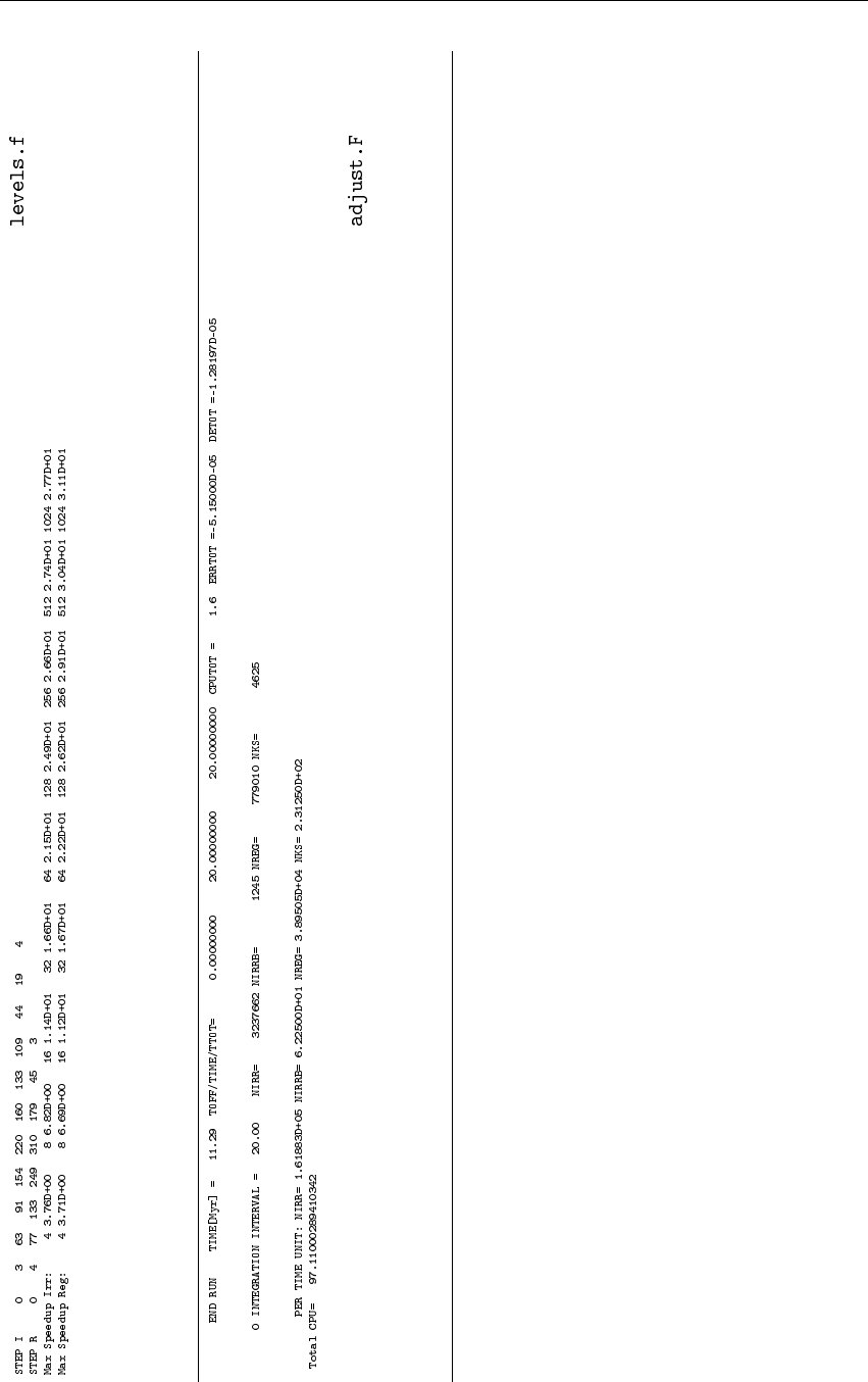
22 6 How to read the diagnostics
6 How to read the diagnostics
The diagnostics is the ASCII readable text printed on unit 6 stdout (“out1000” in Chapter 3) that gives a brief overview of the global status and progress
of the cluster simulation. Different routines write into that file, depending on the options chosen as the input variables. The following lines occur:
written by the routine:
Usage: Repetition of the
input variables
IMF power law index, max. mass, min. mass, total mass, # of primordial bin., metallicity, evolution. epoch [Myrs].
..................................................................
number of objects, mass range, average mass before scaling.
,
(if KZ(20)=0 &
BODY16=BODYN)
or
, if KZ(20)≥2
Information about initial
mass function (IMF).
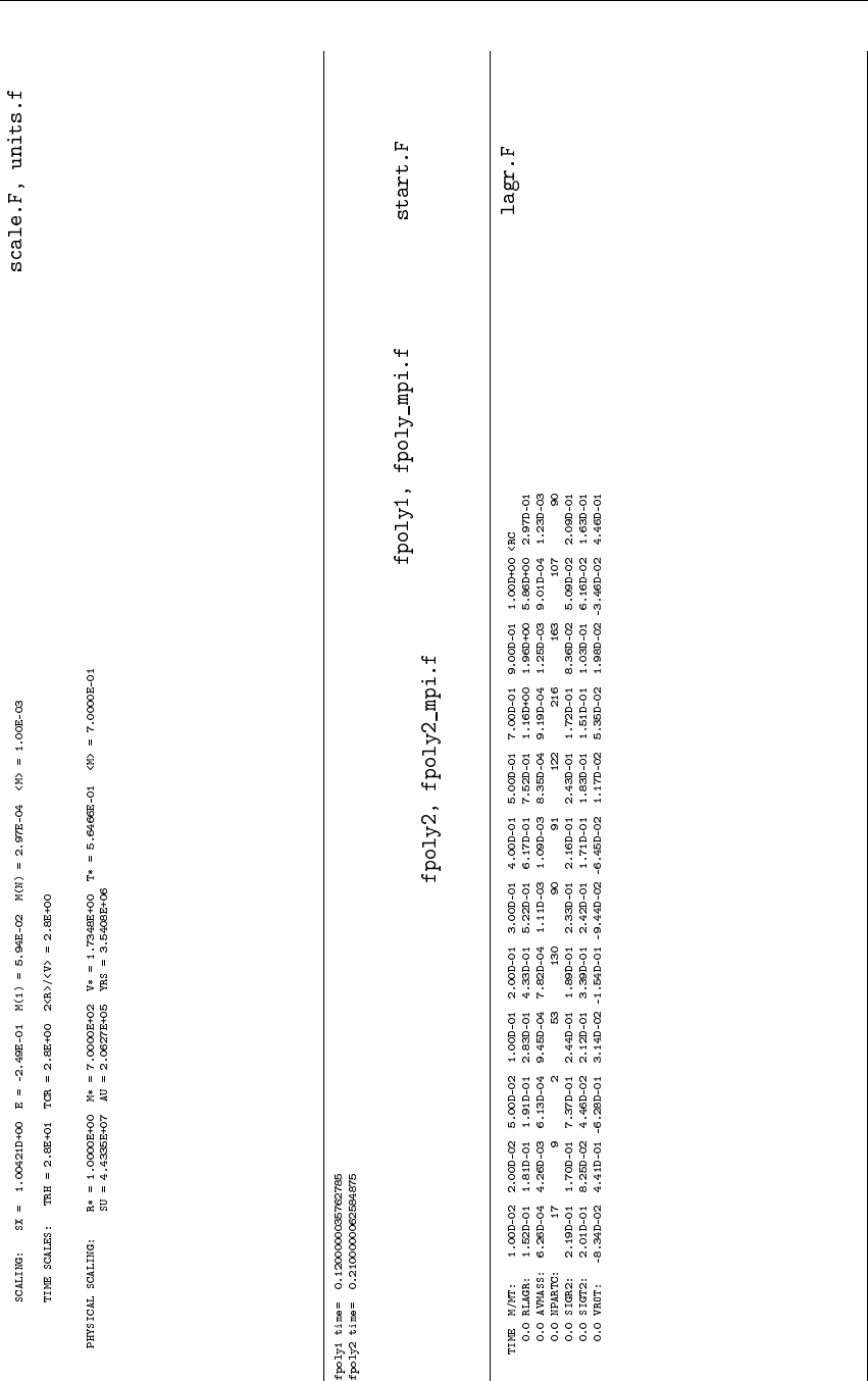
23
scaling factor for energy, total energy, max. mass, min. mass, average mass after scaling;
Spitzer’s half-mass relaxation time, crossing time obtained from total energy and mass, crossing time obtained from
virial radius (see 12);
information about physical scaling: values of one N–body unit in length (pc), mass (solar masses), velocity (km/s),
time (million years), average mass of particles (solar massses), astronomical units (one N–body unit) and years (one
N–body unit).
CPU (wall clock in parallel execution) time for initialising the force and its time derivative ( )
and the second and third time derivative of the force ( ). The mpi-versions are called for
initialisation in case of parallel runs.
Time, specification of the Lagrangian radii, core radius
Time, Lagrangian radii, core radius (if primordial binaries: separately for singles and binaries, not shown above)
Time, average mass between Lagrangian radii, avmass in the core
Time, number of particles within the shell, in the core
Time, radial velocity dispersion within the shell, in the core
Time, tangential vel. dispersion within the shell, in the core
Time, rotational vel. within the shell, in the core (not shown above)
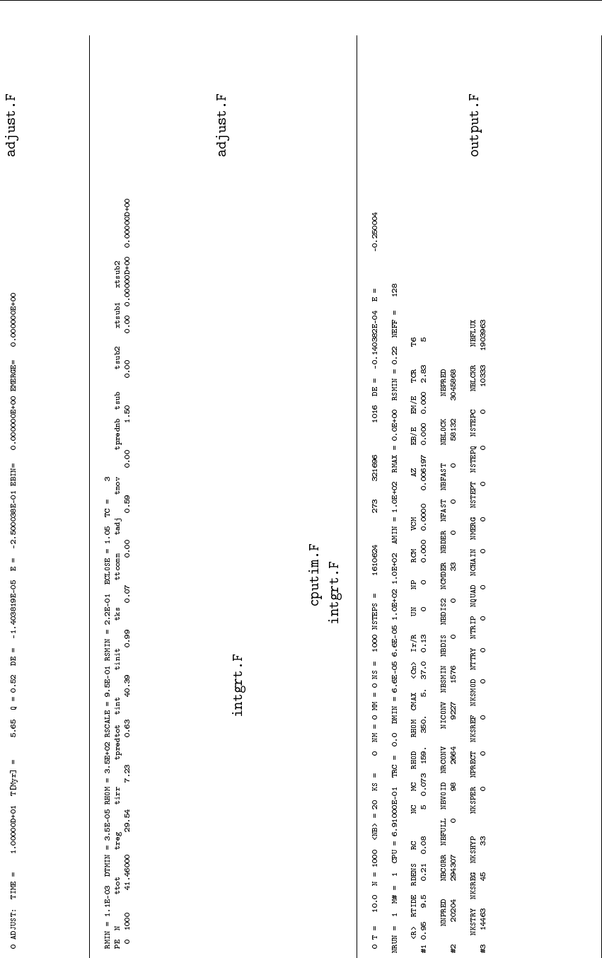
24 6 How to read the diagnostics
rank, “ADJUST:”, total time in NB units, physical time, virial ratio, relative energy error, total energy, total energy of
regularized pairs, energy of mergers
close encounter distance and minimum time step (for regularization search, updated from input parameters if
KZ(16)=1), maximum density, virial radius, minimum neighbour sphere, hard binary threshold energy, total run time
in units of initial crossing times
number of processors, number of particles, total processing time, total regular processing, total irregular processing,
processing of prediction, time spent in , for initialisation, for KS integration, for communication, for adjust
and energy check, for overhead of moving data in parallel runs, for neighbour predictions, for MPI communication
after irregular (tsub) and regular (tsub2) blocks, number of bytes transferred respectively. From xtsub1/tsub and
xtsub2/tsub2 the sustained bandwidth of MPI communication can be read off. Note, that the determination of these
quantities involves a certain overhead by many calls of per block, so for critically large production runs
one may want to comment these out (most of them in ).
time, actual particle number, average neighbour number, number of KS pairs, number of merged KS pairs, number of
hierarchical subsystems, number of single stars, step numbers (irregular, irr. c.m., regular, KS), relative energy error
since last output, total energy
several more lines uncommented here....
25
histogram of distribution of irregular (STEP I), regular (STEP R)
If there are p step distribution (not appearing here, STEP U, in physical time), statistics of parallel work for irr. and
reg. steps, figures given are theoretical speedups for infinitely fast communication (limit of large block sizes)
This is the regular end of a run giving: the integration time, total cumulative absolute and relative errors, cumulative
number of regular, irregular, KS steps, the step numbers per time unit and the total CPU (wall clock for parallel) time
in minutes.
26 6 How to read the diagnostics
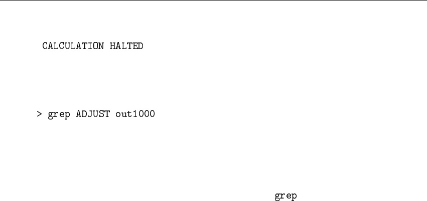
To check a regular stop of the run, look at the end of the diagnostics first. If there are failures,
the line “ ” appears and means that the energy conservation could not be
guaranteed. A restart with smaller steps (ETAI, ETAR) and larger neighbour number NNBOPT
may cure the problem, but not always; persistent problems should be reported to Rainer Spurzem.
The unix command on the output file, e.g.
homedir
produces an overview of the accuracy (energy error at every DTADJ interval). It may show where
problems originated; a restart from the last ADJUST before the error with smaller output intervals
is one way to look after it. Watch out, because sometimes errors are not reproducible, because
changes in ADJUST intervals change frequencies of prediction and small differences can build up.
A quick possibility to see the real evolution of the system is to for the lines with Lagrangian
radii and other quantities (see above), which can directly be plotted, e.g. with gnuplot, because the
first column is always the time.
27
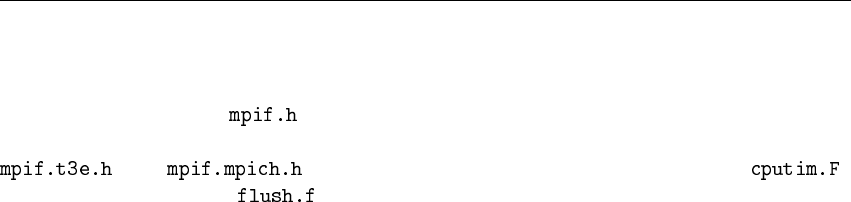
7 Runs on parallel machines
For parallel runs, the file is very important, and system specialists should be consulted
in addition to us what to use. Again, for some standard systems templates are provided (e.g.
or ). The routine providing CPU–time measurements, ,
and the use of the function may need special attention depending on the hardware.
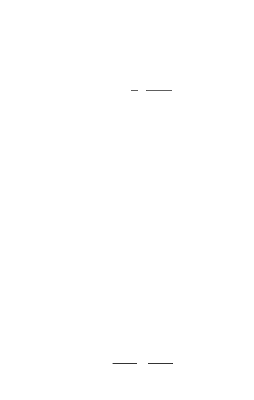
28 8 The Hermite integration method
8 The Hermite integration method
Each particle is completely specified by its mass m, position r0, and velocity v0, where the sub-
script 0 denotes an initial value at a time t0. The equation of motion for a particle iis given by its
momentary acceleration a0,idue to all other particles and its time derivative ˙
a0,ias
a0,i=−∑
i6=j
Gmj
R
R3,(1)
˙
a0,i=−∑
i6=j
GmjV
R3+3R(V·R)
R5,(2)
where Gis the gravitational constant; R=r0,i−r0,jis the relative coordinate; R=|r0,i−r0,j|the
modulus; and V=v0,i−v0,jthe relative space velocity to the particle j.
The Hermite scheme employed in NBODY6++ follows the trajectory of the particle by firstly
“predicting” a new position and new velocity for the next time step t. A Taylor series for ri(t)and
vi(t)is formed:
rp,i(t) = r0+v0(t−t0) + a0,i
(t−t0)2
2+˙
a0,i
(t−t0)3
6,(3)
vp,i(t) = v0+a0,i(t−t0) + ˙
a0,i
(t−t0)2
2.(4)
The predicted values of rpand vp, which result from this simple Taylor series evaluation, using
the force and its time derivative at t0, do not fulfil the requirements for an accurate high–order
integrator; they just give a first approximation to r1and v1at the upcoming time t1. Even if
the time step, t1−t0, is chosen impracticably small, a considerable error will quickly occur, let
alone the inadequate computational effort. Therefore, an improvement is made by the Hermite
interpolation which approximates the higher accelerating terms by another Taylor series:
ai(t) = a0,i+˙
a0,i·(t−t0) + 1
2a(2)
0,i·(t−t0)2+1
6a(3)
0,i·(t−t0)3,(5)
˙
ai(t) = ˙
a0,i+a(2)
0,i·(t−t0) + 1
2a(3)
0,i·(t−t0)2.(6)
Here, the values of a0,iand ˙
a0,iare already known, but a further derivation of equation (2) for
the two missing orders on the right hand side turns out to be quite cumbersome. Instead, one
determines the additional acceleration terms from the predicted (“provisional”) rpand vp; we
calculate their acceleration and time derivative according to the equations (1) and (2) anew and
call these new terms ap,iand ˙
ap,i, respectively. Because these values ought to be generated by
the former high–order terms also (which we avoided), we put them into the left–hand sides of (5)
and (6). Solving equation (6) for a(2)
0,i, then substituting it into (5) and simplifying yields the third
derivative:
a(3)
0,i=12a0,i−ap,i
(t−t0)3+6˙
a0,i+˙
ap,i
(t−t0)2.(7)
Similarly, substituting (7) into (5) gives the second derivative:
a(2)
0,i=−6a0,i−ap,i
(t−t0)2−22˙
a0,i+˙
ap,i
t−t0
.(8)

29
Note, that the desired high–order accelerations are found just from the combination of the low–
order terms for r0and rp. We never derived higher than the first derivative, but achieved the higher
orders easily through (1) and (2). This is called the Hermite scheme.
Previously, a four–step Adams–Bashforth–Moulton integrator was used (especially in NBODY5,
[2]), however, the new Hermite scheme allows twice as large timesteps for the same accuracy. Also
its storage requirements are less [16], [17], [4], [5].
Finally, we extend the Taylor series for ri(t)and vi(t), eqs. (3) and (4), by two more orders,
and find the “corrected” position r1,iand velocity v1,iof the particle iat the computation time t1as
r1,i(t) = rp,i(t) + a(2)
0,i
(t−t0)4
24 +a(3)
0,i
(t−t0)5
120 ,(9)
v1,i(t) = vp,i(t) + a(2)
0,i
(t−t0)3
6+a(3)
0,i
(t−t0)4
24 .(10)
The integration cycle for other upcoming steps may now be repeated from the beginning, eqs. (1)
and (2). The local error in rand vwithin the two time steps ∆t=t1−t0is expected to be of order
O(∆t5), the global error for a fixed physical integration time scales with O(∆t4)[15].

30 9 Individual and block time steps
9 Individual and block time steps
Stellar systems are characterized by a huge dynamical range in radial and temporal scales. The
time scale varies e.g. in a star cluster from orbital periods of binaries of some days up to the relax-
ation of a few hundred million years, or even billions of years. Even if we put for a moment the
very close binaries aside, which are treated differently (by regularization methods), there typically
is a large dynamic range in the average local stellar density from its centre to the very outskirts,
where it dissolves into the galactic tidal field. In a classical picture, the two closest bodies would
determine the time–step of force calculation for the whole rest of the system. However, for bodies
in regions where the changes of the force are relatively small, a permanent re–computing of the
terms appears time consuming. So, in order to economize the calculation, these objects shall be
allowed to move a longer distance before a recomputation becomes necessary. In between there
is always the possibility to acquire particle positions and velocities via a Taylor series prediction,
as described in Chapter 8. This is the idea of a vital method for assigning different time–steps,
∆t=t1−t0, between the force computations, the so–called “individual time–step scheme” [1],
which was later advanced to the hierarchical block steps.
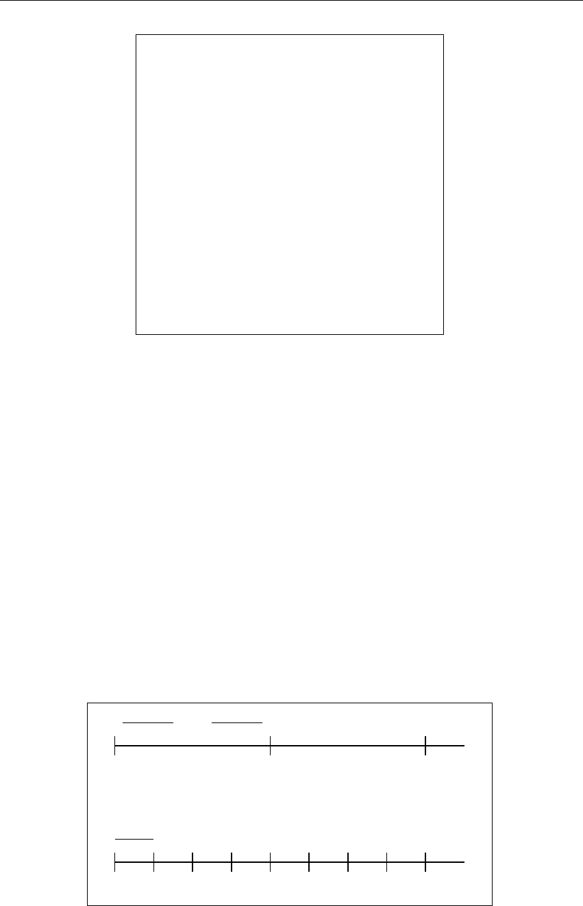
0 1 2 4 8 time steps 16
------------ - -
- - - - - -
- - - - - - - -
- -
i
k
l
m
particles
Figure 9.1: Block time steps exemplary for four particles.
Each particle is assigned its own ∆tiwhich is first illustrated for the case of “block time–steps”
in Figure 9.1. The particle named ihas the smallest time step at the beginning, so its phase space
coordinates are determined at each time step. The time step of kis twice as large as i’s, and its
coordinates are just extrapolated (“predicted”) at the odd time steps, while a full force calculation
is due at the dotted times. The step width may be altered or not after the end of the integration
cycle for the special particle, as demonstrated for kand lbeyond the label “8”. The time steps
have to stay commensurable with both, each other as well as the total time, such that a hierarchy
is guaranteed. This is the block step scheme.
As a first estimate, the rate of change of the acceleration seems to be a reasonable quantity for
the choice of the time step: ∆ti∝pai/˙
ai. But it turns out that for special situations in a many-body
system, it provides some undesired numerical errors. After some experimentation, the following
formula was adopted [2]:
∆ti=v
u
u
tη|a1,i||a(2)
1,i|+|˙
a1,i|2
|˙
a1,i||a(3)
1,i|+|a(2)
1,i|2,(11)

31
where ηis a dimensionless accuracy parameter which controls the error. In most applications it is
taken to be η≈0.01 to 0.02, see also next chapter.
For the block–time steps, the synchronization is made by taking the next–lowest integer of ∆ti;
the time steps are quantized to powers of 2 [15]. Then, there will be a group (block) of several
particles which are due to movement at each time step. If one keeps the exact ∆ti’s evaluated
from (11) for each particle, the commensurability is destroyed, and we arrive at the so–called
“individual time steps”; in this case, there exists one sole particle being due. The latter concept
is realized in the earlier codes NBODY1, NBODY3, NBODY5, where a neighbour scheme is
renounced. NBODY4, NBODY6, and NBODY6++ use a block step scheme.
Subsystems like star binaries, triples or a similar subgroups (they are termed KS pairs, chains,
hierarchies) enter the time–step scheme with their respective centre’s of masses only. Their inter-
nal motion is treated in a different way by a regularized integration (Chapter 11).

32 10 The Ahmad–Cohen scheme
10 The Ahmad–Cohen scheme
The computation of the full force for each particle in the system makes simulations very time–
consuming for large memberships. Therefore, it is desirable to construct a method in order to
speed up the calculations while retaining the collisional approach. One way to achieve this is to
employ a “neighbour scheme”, suggested by [9].
The basic idea is to split the force polynomial (5) on a given particle iinto two parts, an
irregular and a regular component:
ai=ai,irr +ai,reg.(12)
The irregular acceleration ai,irr results from particles in a certain neighbourhood of i(in the code,
FI and FIDOT are the irregular force and its time derivative at the last irregular step; internally
some routines use FIRR and FD as a local variable). They give rise to a stronger fluctuating
gravitational force, so it is determined more frequently than the regular one of the more distant
particles that do not change their relative distance to iso quickly (in the code, FR and FRDOT
are the regular force and its time derivative at the last regular step; some routines use as a local
variable FREG and FDR). We can replace the full summation in eq. (1) by a sum over the Nnb
nearest particles for ai,irr and add a distant contribution from all the others. This contribution is
updated using another Taylor series up to the order FRDOT, the time derivative of FR at the last
regular force computation1.
Wether a particle is a neighbour or not is determined by its distance; all members inside a
specified sphere (“neighbour sphere” with radius rs) are held in a list, which is modified at the end
of each “regular time–step” when a total force summation is carried out. In addition, approaching
particles within a surrounding shell satisfying R·V<0 are included. This “buffer zone” serves
to identify fast approaching particles before they penetrate too far inside the neighbour sphere.
The neighbour criterion should be improved according to relative forces rather than distances, in
particular, if there are very strong mass differences between particles (black holes!) — such kind
of work is under progress.
Figures 10.1 and 10.2 show how the Ahmad–Cohen scheme works for one particle [17]. At
the beginning of the force calculation, a list of neighbour objects around the particle iis created
first (filled dots). From this neighbour list the irregular component ai,irr is calculated, and then the
summation is continued to the distant particles obtaining ai,reg. At the same time we also calculate
the first time derivative. From the equations (5) and (6) the position and velocity of the particle
iare predicted. At time t1,irr we apply the “corrector” only for ai,irr from the neighbours; the
regular component we do not correct, but obtain by extrapolating ai,reg. At the next step, t2,irr, the
same predictor–corrector method proceeds for the neighbour particles, while the correction of the
distant acceleration term is still neglected. When t1is reached, the total force is calculated on the
basis of the full application of the Hermite predictor–corrector method. Also, a new neighbour list
is constructed using the positions at time t1. Thus, we calculate at certain times only the forces
from neighbours (irregular time–step, tirr), while at other times we calculate both the forces from
neighbours and distant particles (regular time–step, treg).
For a neighbour list of size Nnb N, this procedure can lead to a significant gain in efficiency,
provided the respective time scales for ai,irr and ai,reg are well separated.
1Note, that the code also keeps the variables F and FDOT, which contain one half (!) of the total force, and one
sixth (!) of the total time derivative of the force; this just a handy assignment for the frequent predictions of equation 3.
33
∗
•
•
•
•
••
•
•
rs
◦
◦
◦ ◦◦
◦◦ ◦◦
◦
◦
◦
◦
◦
◦
◦
◦◦
◦
◦
◦
◦
◦
◦
◦
◦
◦◦◦ ◦
Figure 10.1: Illustration of the neighbour scheme for particle imarked as the asterisk (after [2]).
The actual size of neighbour spheres in NBODY6++ is controlled iteratively by a requirement
in order to keep a certain optimal number of neighbours. This variable, NNBOPT, can be adjusted
according to performance requirements. Its typical values are between 50 and 200 for a very
wide range of total particle numbers N. Outside of the half-mass radius, the requirement of having
NNBOPT neighbours is relaxed due to low local densities. Insisting on NNBOPT neigbours could
result in undesired large amplitude fluctuations of the neighbour radii.
While [18] claim that the optimal neighbour number should grow as N3/4(which would be
unsuitable for the performance on parallel computers), this is still an unsettled question. [2] advo-
cates the coupling of the neighbour radius to the local density contrast, but NBODY6++ does not
use that, since it makes average neighbour numbers much less predictable, which is bad for the
performance and profiling issues on supercomputers, again.
Resuming, the method of the two particle groups is squeezed into the hierarchical time–step
scheme making the overall view quite complex. Each particle is moved due to its time–step order
and the time–steps, because the force calculation is divided: In eq. (11) a further subscript is
needed which distinguishes the regular and irregular time step. The accuracy can be tuned by
t1,irr t2,irr ... t1∗,irr t2∗,irr
t0t1t2
-
∆tirr
∆treg -
Figure 10.2: Regular and irregular time steps (after [17]).

34 10 The Ahmad–Cohen scheme
ηirr ≈0.01 and ηreg ≈0.02, again.
Both, the neighbour scheme and the hierarchical time–step scheme have in common that they
are centered on one particle i, and they distinguish between nearby and remote stars, and they
save computational time. One may ask: What is the intriguing difference between them? — The
neighbour scheme is a spatial hierarchy, which avoids a frequent force calculation of the remote
particles, because their totality provides a smooth potential which does not vary so much with
respect to the particle i; that potential is rather superposed by some fluctuating peaks of close–by
stars which will be “worked in” by the more often force determination. The time step scheme,
in contrast, exhibits the temporal behaviour of the intervals for re–calculation of the full force
in order to maintain the exactness of the trajectory; time steps chosen too small slow down the
advancing calculation losing the computer’s efficiency.
35
11 KS–Regularization
The fourth main feature of the codes since NBODY3 is a special treatment of close binaries. A
close encounter is characterised by an impact parameter that is smaller than the parameter for a 90
degree deflection
p90 =2G(m1+m2)/v2
∞(13)
where G,m1,m2,v∞are the gravitational constant, the masses of the two particles and their relative
velocity at infinity. In the cluster centre, it is very likely that two (or even more) stars come very
close together in a hyperbolic encounter. As the relative distance of the two bodies becomes small
(R→0), their timesteps are reduced to prohibitively small values, and truncation errors grow due
to the singularity in the gravitational potential, eqs. (1) and (2). In the NBODY code, the parameter
RMIN is used to define a close encounter, and it is kept to the value of equation 13 (if KZ(16) > 0
is chosen in the control parameters). The corresponding time step DTMIN can be estimated from
dtmin =κhη
0.03ir3
min
hmi1/2
(14)
where κis a free numerical factor, ηthe general time step factor, and hmithe average stellar mass
[2]. If two particles are getting closer to each other than RMIN, and their time steps getting smaller
than DTMIN, then they are candidates for “regularization”.
Regularization is an elegant trick in order to deal with such particles which are as close as the
diamond in the Figure 10.1. The idea is to take both stars out of the main integration cycle, replace
them by their centre of mass (c.m.) and advance the usual integration with this composite particle
instead of resolving the two components. The two members of the regularized pair (henceforth KS
pair) will be relocated to the beginning of all vectors containing particle data, while at the end one
additional c.m. particle is created (see below). One of the purposes of the code variable NAME(I)
is to identify particles after such a reshuffling of data.
To be actually regularized, the two particles have to fulfil two more sufficient criteria: that they
are approaching each other, and that their mutual force is dominant. In the equations in routine
, these sufficient criteria are defined as
R·V>0.1p(G(m1+m2)R
γ:=|apert|·R2
G(m1+m2)<0.25
Here, apert is the vectorial differential force exerted by other perturbing particles onto the two
candidates, R,R,Vare scalar and vectorial distance and relative velocity vector between the two
candidate, respectively. The factor 0.1 in the upper equation allows nearly circular orbits to be
regularized; γ<0.25 demands that the relative strength of the perturbing forces to the pairwise
force is one quarter of the maximum. These conditions describe quantitatively that a two-body
subsystem is dynamically separated from the rest of the system, but not unperturbed.
The internal motion of a KS pair will be determined by switching to a different (regularized)
coordinate system. This transformation can be traced back to the square in quaternion space, where
— by sacrificing some commutativity rules — it is guaranteed that the real-space motion does not
leave the three-dimensional Cartesian space. It involves a set of four regular spatial coordinates
and a fictitious time s(t), obtained in its simplest variant by the transformation dt =Rds. Any
unperturbed two–body orbit in real space is mapped onto a harmonic oscillator in KS–space with
double the frequency. Since the harmonic potential is regular, numerical integration with high
accuracy can proceed with much better efficiency, and there is no danger of truncation errors for
36 11 KS–Regularization
arbitrarily small separations. The internal time–step of such a KS–regularized pair is independent
of the eccentricity and, depending on the parameter ETAU, of the order of some 50–100 steps
per orbit. The method of regularization goes back to [14] and makes an accurate calculation of a
perturbed two–body motion possible. A modern theoretical approach to this subject can be found
in [25]; the Hamiltonian formalism of the underlying transformations is nicely explained in [20].
While regularization can be used for any analytical two–body solution across a mathematical
collision, it is practically applied to perturbed pairs only. Once the perturbation γfalls below
a critical value (input parameter GMIN ≈10−6), a KS–pair is considered unperturbed, and the
analytical solution for the Keplerian orbit is used instead of doing numerical integration. A little
bit misleading is that such unperturbed KS–pairs are denoted in the code as ”mergers”, e.g. in the
number or merges (NM) and the energy of the mergers (EMERGE). Merged pairs can be resolved
at any time if the perturbation changes. The two–body KS regularization occurs in the code either
for short-lived hyperbolic encounters or for persistent binaries.
In the code, the KS–pair appears as a new particle at the postion of the centre of mass. The
variable NTOT, that contains the total number of particles Nplus the c.m.’s, is increased by 1.
When the pair is disrupted, NTOT is decreased again. The maximum number of possible KS–
pairs is saved in the variable KMAX, which sets a threshold for the extension of the vector NTOT
(see Chapter 5).
Close encounters between single particles and binary stars are also a central feature of clus-
ter dynamics. Such temporary triple systems often reveal irregular motions, ranging from just a
perturbed encounter to a very complex interaction, in which disruption of binaries, exchange of
components and ejection of one star may occur. Although not analytically solvable, the general
three–body problem has received much attention. So, the KS–regularization was expanded to the
isolated 3– and 4–body problem, and later on to the perturbed 3–, 4–, and finally to the N–body
problem. The routines are called
•(unperturbed 3-body subsystems, [8]),
•(unperturbed 4-body subsystems), and
•with different stages of implementation (slow-down, Stumpff functions, see for
consecutive references Mikkola & Aarseth 1990, 1993, 1996, 1998, and [20]).
While occurrences of “triple” and “quad” will be rare in a simulation, the chain regularization is
invoked if a KS–pair has a close encounter with another single star or another pair. Especially,
if systems start with a large number of primordial binaries, such encounters may lead to stable
(or quasi-stable) hierarchical triples, quadruples, and higher multiples. They have to be treated
by using special stability criteria. Some of them are actually already implemented, but there is
ongoing research and development in the field.
A typical way to treat all such special higher subsystems is to define their c.m. to be a pseudo-
particle, i.e. a particle with a known sub-structure (very much like nodes in a TREE code). The
members of the pseudo-particles will be deactivated by setting their mass to zero (ghost particles).
At present there can only exist one chain at a time in the code, while merged KS binaries, and
hierarchical subsystems can be more frequent. Details of these procedures are beyond the scope
of this introductory manual.
Every subsystem — KS pair, chain or hierarchical subsystem — is perturbed. Perturbers are
typically those objects that get closer to the object than Rsep =R/γ1/3
min , where Ris the typical size
of the subsystem; for perturbers, the components of the subsystem are resolved in their own force
computation as well (routines , ).

37
12 Nbody–units
The NBODY–code uses Dimensionless units, so–called “Nbody units”. They are obtained when
setting the gravitational constant Gand the initial total cluster mass Mequal to 1, and the initial
total energy Eto −1/4 (see [12], [7]).
Since the total energy Eof the system is E=K+Wwith K=1
2Mhv2ibeing the total kinetic
energy and W=−(3π/32)GM2/Rthe potential energy of the Plummer sphere, we find from the
virial theorem that
E=1
2W=−3π
64
GM2
R.(15)
Ris a quantity which determines the length scale of a Plummer sphere. Using the specific defini-
tions for G,M, and Eabove, this scaling radius becomes R=3π/16 in dimensionless units. The
half mass radius rhcan easily be evaluated by the formula (e.g. [26]):
M(r) = Mr3/R3
(1+r2/R2)3/2(16)
when setting M(rh) = 1
2M. It yields rh= (22/3−1)−1/2R=1.30 R. The half–mass radius is located
at R=0.766, or about 3/4 “Nbody–radii”.
The virial radius of a system is defined by Rvir =GM2/2|W|, while the r.m.s. velocity is
hv2i1/2=2K/M. In virial equilibrium |W|=2K, so it follows for the crossing time
tcr :=2Rvir
hv2i1/2=GM5/2
(2|E|)3/2.(17)
The setting of G=M=1 and E=−0.25 also determines the unit of time; so it follows that
tcr =2√2 in N-body units. By inversion we have
τNB =GM5/2
(4|E|)3/2,(18)
for the unit of time τNB. The virial radius of Plummer’s model is Rvir =1 in N-body units.

38 13 Output
13 Output
Table 17: Definition of parameters
Global properties
TIME time of simulation
RSCALE Half mass radius
RTIDE Tidal radius
RC Core radius
NC Number of stars inside core radius
MC Core mass
VC r.m.s velocity inside core radius
CMAX Maximum number density / half mass mean value
RDENS(1:3) Density center position
RHOD Density weighted average density ΣRHO2/ΣRHO
RHOM Maximum mass density / half mass mean value
hMiAverage mass of star
M1 Mass of most massive star
ZMASS Total mass of cluster
MODEL Snapshot counter in output
NRUN Run identification index
TIDAL4 Twice angular velocity for linearised tidel force
Energy
DE relative energy error
DELTA absolute energy error
BE(1) Intial total energy
BE(2) Last adjust total energy
BE(3) Current total energy
ZKIN Kinetic energy
POT Potential energy
ETIDE Tidal energy
ETOT Total energy
E Mechanical energy: ZKIN - POT + ETIDE (E(3))
ESUB Binding energy of unperturbed triples and quadruples
EMERGE Binding energy of mergers (E(9))
EBIN Binding energy of KS binaries
ECOLL The difference of binding energy of inner binary at the end and begin
of hierarchical systems (E(10))
EMDOT Mechanical energy of mass loss due to stellar evolution (E(12))
ECDOT Energy of velocity kick due to stellar evolution
ECH Binding energy of chain
EBINP Primordial KS binary energy (E(1))
EBINN Energy of new KS binary formed by dynamics (E(2))
EESCS Single escaper mechanical energy (E(4))
EESCPB Binding energy of primordial KS binary escapers (E(5))

39
EESCPC Mechanical energy of center mass of primordial KS binary escapers
(E(6))
EESCNB Binding energy of new formed KS binary escapers (E(7))
EESCNC Mechanical energy of center mass of new KS binary escapers (E(8))
Scaling factors (Astronomical units = N–body units ×scaling factor)
RBAR PC
TSCALE Myr
TSTAR Myr
VSTAR km/s
RAU AU
ZMBAR Solar mass
SU Solar radius
Astronomical units
R* Solar radius
L* Solar luminosity
M* Solar mass
Status number
NTOT Total number of particles (include all binary components, single stars
and center of mass)
N Total number of stars (binary counts as two stars)
NS Single star number
NPAIRS Number of KS regularization pairs
NMERGE Number of mergers (stable triples)
MULT Number of ≥4 bodies merger
NZERO Initial particle number (2* binaries + singles, initial N)
NB0 Primordial binary number
NUPKS Unperturbed KS
NPKS Total perturber number of KS
NTYPE(1:16)Number of stars with type 1 to 16
For stars
I Index of star (position in particle data array)
NAME Identification of individual star, it’s constant and unique value for each
star (exclude un-physical particles like center mass and ghosts) during
the whole simulation
K* KSTAR type:
-1: Pre-main sequence.
0: Low main sequence (M < 0.7).
1: Main sequence.
2: Hertzsprung gap (HG).
3: Red giant (RG) branch.
4: Core Helium burning.
5: First Asymptotic giant branch (AGB).
6: Second AGB.
7: Helium main sequence.
8: Helium HG.
9: Helium giant branch.

40 13 Output
10: Helium white dwarf.
11: Carbon-Oxygen white dwarf.
12: Oxygen-Neon white dwarf.
13: Neutron star.
14: Black hole.
15: Massless supernova remnant.
M Mass of star
X(1:3) Three dimension position
V(1:3) Three dimension velocity
DM Current mass loss due to stellar evolution (N–body units)
DMA Accumulated mass loss due to stellar evolution
STEP Irregular time step of star
STEPR Regular time step of star
ZKIN Kinetic energy
POT Potential
NB Neighbor number
RNB Neighbor radius
RHO Mass density of individual star calculated by nearest 5 neighbors, (only
avaiable for particles inside core radius
Stellar evolution of star
RS star radius
L luminosity
Teff effective temperature
ROT angular velocity of star
For binaries
SEMI semi-major axis
ECC eccentricity
PERI Pericenter distance
R12 distance between two members of binary
RI distance to density center
VI velocity of center of mass
P Orbit period
I1/I2 Index for binary component 1/2 (Not always equal name)
ICM Index for center mass particle (Not always equal name)
NP perturber number
H Binary energy per unit mass
EB Binary energy: M(I1)*M(I2)/M(ICM)*H
GAMMA Perturbation on KZ binary
IPAIR Pair index for binary
STEP(I1) KS time step of binary
TC circularization timescale for current pericenter
FLAG-PB Primordial binary indicator. -1: Primordial bianry; 0: New binary
INEW Index of new star generated by binary collision or coalescence
For hierarchical systems
IM merger index
IMC Number count of current merger

41
INPAIR Index of inner binary
INCM Inner binary center mass index
NAME(IM) Merger center mass name
I1/I2 Inner binary two component indexs
I3 Outer particle index
ECC0 Inner binary orbit eccentricity
ECC1 Outer orbit eccentricity
EB0 Inner binary energy
EB1 Outer orbit energy
P0 Inner binary orbit period
P1 Outer orbit period
R12 Inner binary components seperation
RIN3 Separation between inner center mass and outer component
TG Inner orbit eccentricity growth timescale
ECCMIN Minimum eccentricity of inner binary orbit
ECCMAX Maximum eccentricity of inner binary orbit
PERIM smallest pericenter distance of outer particle orbit
PCR Stability triple system criterion for PERIM (assess.f), the real stability
criterion is more complicated and depend on the ECC1
SEMI0 Inner binary orbit semi-major axis
SEMI1 Outer orbit semi-major axis
INA Inclination angle in unit degree
FLAG-H Hierarchical system indicator. -1: merger, triple, chaotic binary, tidal
circularization binary...; 0: normal binary
For quadruple systems
OCM Outer binary center of mass index
OCPAIR Index of outer binary
I3/I4 Outer binary two component index
ECC2 Outer binary eccentricity
EB2 Outer binary energy
SEMI2 Outer binary orbit semi-major axis
R34 Outer binary components seperation
DP34 Difference potential correction for the outer binary
For chain
IC Chain index
NCH Number of chain members
ECH Total energy of perturbed system (N-body interface)
NP Perturbers of chain
ENERGY Total energy of chain
RSUM Sum of all chain distances
RGRAV Gravitational radius ((sum M(I)*M(J))/ABS(ENERGY))
TCR Local crossing time ((sum M(I))**2.5/ABS(2*ENERGY)**1.5)
RMAXS Maximum size of unperturbed configuration
RIJ(i-j) Distance between member i and j
ICM1 First binary index after termination
ICM2 Second binary index after termination

42 13 Output
For kick
M0 mass before kick
MN mass after kick
VK kick velocity after limit check
VI Initial velocity of kick star in cluster
VF Final velocity of kicked star in cluster
VK0 Kick velocity generated from Henon’s method (Douglas Heggie
22/5/97)
FB Fallback ratio, VK = VK*(1-FB)
VESC cluster escape velocity
VDIS escape velocity from binary system: SQRT(2*M(ICM)/R12)
Table 18: Notice for Table19
File format
Header-* The Header of file with line number *, the description of it is shown in
the right cell
H-Label-* Content labels are shown at the line number *, data begin from the next
line
F-Label Content labels are shown at the beginning of each line
I-Label Content labels are shown before each data
N-Label No labels in file
Frequency (freq.)
Tevent Output when event is triggered
T0Output during initialization
∆Tout Output time interval (input parameter DELTAT)
∆Tad j Adjust time interval (input parameter DTADJ)
∆THR Stellar evolution output time interval (input parameter DTPLOT)
NFIX Frequency of output (input parameter)
option
#[num]KZ option [num]
klogical or
&& logical and
CHAIN Use chain: #15 >0&&(#30 >0k#30 =−1)
USE_GPU switch on GPU during compiling code
USE_HDF5 switch on HDF5 during compiling code
Table19 show all output files of NBODY6++. The filename will be named as “[name].[unit]”. The
first column [name] with suffix “*” means this file will output as seperated snaphshots split by
TIME[NB] (shown as suffix of file name).
Table 19: Output file information
name unit code option freq. content

43
conf* 3 output.F #3 >0∆Tout
×
NFIX
Basic data snapshots
Header-1 NTOT, MODEL, NRUN, NK
Header-2 TIME[NB], NPAIRS, RBAR, ZMBAR, RTIDE, TIDAL4, RDENS(1:3),
TIME/TCR, TSCALE, VSTAR, RC, NC, VC, RHOM, CMAX,
RSCALE, RSMIN, DMIN1
N-Label M, RHO, XNS, X(1:3), V(1:3), POT, NAME (All in NB unit)
Notice the file is unformatted (binary file). Each item output continually from 1 to NTOT.
All items output in one line after two header lines.
NK : The number of parameters in Header-2, right now is always 20
TCR : Crossing time
RSMIN : Smallest neighbor radius obtained in last output (output.F) time
DMIN1 : Smallest two body distance
XNS : The fifth nearest neighbor distance, (only avaiable for particles inside core radius
degen 4 degen.f #9 ≥3Tevent Binary with degenerate stars
Header-1 RBAR, hMi[M*], M1[M*], TSCALE, NB0, NZERO
H-Label-2 ICASE, TIME[Myr], SEMI[AU], ECC, PERI/RS, P[days], RI[PC],
M(I1)[M*], M(I2)[M*], K*(I1),K*(I2),K*(ICM), NAME(I1),NAME(I2)
ICASE: 3: normal binary; 4: CE binary; 5: physical collision binary
PERI/RS: Pericenter / maximum stellar radius of two members
lagr 7 lagr.f #7 ≥3∆Tout Lagrangian radii, average mass, aver-
age velocity, velocity dispersion out-
put (calculation of Lagrangian radii
use initial total mass of cluster)
Header-1 Labels and column number for each output
H-Label-2 Rlagr,Rlagr,s,Rlagr,b,hMi,NShell ,hVxi,hVyi,hVzi,hVi,hVri,hVti,σ2,
σ2
r,σ2
t,hVrot.i(All in NB units)
For each items above, there are 18 columns with different mass fraction(%): 0.1, 0.3, 0.5,
1, 3, 5, 10, 20, 30, 40, 50, 60, 70, 80, 90, 95, 99, 100 and inside core radius (exclude
Rlagr,s,Rlagr,b)
Rlagr: Lagrangian radius
Rlagr,s: Single star Lagrangian radius
Rlagr,b: KZ binaries Lagrangian radius
hMi: Average mass of a spherical shell defined by Rlagr
hVx/y/zi: Mass weighted average velocity in x/y/z direction
hVti: Mass weighted average tangential velocity
hVri: Mass weighted average radial velocity
σ2: Mass weighted velocity dispersion square
σ2
r: Mass weighted radius velocity dispersion square
σ2
t: Mass weighted tangential velocity dispersion square
hVrot.i: Mass weighted average rotational velocity projected in x-y plane
bdat 8 ksin2.f #8 >0Tevent New hierarchical (B-S)-S binary in-
formation
ksinit.F #8 >0 New binary information
ksterm.F #8 >0 End binary information

44 13 Output
I-Label TIME[NB], NAME(I1) NANE(I2), FLAG-PB, M(I1)[NB], M(I2)[NB],
EB[NB], SEMI[NB], R12[NB], GAMMA[NB], RI[NB]
bdat* 9 bindat.f #8 ≥2∆Tout KS binary output
Header-1 NPAIRS, MODEL, NRUN, N, NC, NMERGE, TIME[NB],
RSCALE[NB], RTIDE[NB], RC[NB], TIME[Myr], ETIDC[NB],
0
Header-2 EBINP, EBINN, E, EESCS, EESCPB, EESCPC, EESCNB, EESCNC,
EMERGE, ECOLL (All in NB unit)
Header-3 SBCOLL, BBCOLL, ZKIN, POT, EBIN0, EBIN, ESUB, EMERGE,
BE(3), ZMASS, ZMBIN, CHCOLL, ECOLL (All in NB unit)
H-Label-4 NAME(I1), NAME(I2), M1[M*], M2[M*], E[NB], ECC, P[days],
SEMI[AU], RI[PC], VI[km/s], K*(I1), K*(I2), ZN[NB], RP[NB],
STEP(I1)[NB], NAME(ICM), ECM[NB], K*(ICM)
ETIDC[NB]: escape energy due to tidal force
SBCOLL: The difference of binding energy of inner binary at the end and begin of unper-
turbed triples
BBCOLL: The difference of binding energy of inner binary at the end and begin of un-
perturbed B-B quadruples
ZMBIN : Total KS binary masses
CHCOLL: The difference of binding energy of inner binary at the end and begin of chain
dat 10 start.F #22 =1T0Basic data after initialization
N-label M[NB], X(1:3)[NB], V(1:3)[NB]
esc 11 escape.f #23 =2,
4
∆Tad j escaping star output
H-Label-1 TIME[Myr], M[M*], EESC, VI[km/s], K*, NAME
EESC: dimensionless escape energy
hiarch 12 hiarch.f #18 =1,
3
Tevent New/End stable hierarchical system
(mergers) information
Header-1 RBAR, hMi[M*], M1[M*], TSCALE, NB0, NZERO
F-Label TIME, SEMI0, SMEI1, ECC1, PERI0, PERI0M, P1/P0,
M(INCM)/M(I3), PCR/SEMI0, M(INCM)/<M>, MR, INA, NAME(I1),
NAME(I2), NAME(I3), K*(INCM), ECC0, ECCMIN, ECCMAX,
K*(I1), K*(I2), RSM (All in NB unit)
F-Label TIME RI/RC, SEMI0, ECC0, PERI0, P0F/P0I, RC/RSCALE,
GAMMA(INCM), NKI, NKF, NPAIRS, NAME(I2) (All in NB unit)
PERI0: Inner binary pericenter distance
PERI0M: Inner binary minimum pericenter distance
MR: Mass ratio of inner binary components (>1)
PSM: Maximum stellar radius of two members of inner binary
P0F/P0I: Period of inner binary at the end of merger over at the beginning of merger
NKI: Orbit number the inner binary during the life of merger over the period of inner
binary at the beginning of merger
NKF: Orbit number the inner binary during the life of merger over the period of inner
binary at the end of merger

45
coll 13 mix.f #19 ≥3Tevent Mixed star (physical collision of bi-
nary without evolved stars) informa-
tion
Header-1 RBAR, hMi[M*], M1[M*], TSCALE, NB0, NZERO
H-Label-2 TIME[NB], NAME(I1), NAME(I2), K*(I1), K*(I2), K*(INEW),
M(I1)[M*], M(I2)[M*], M(INEW)[M*], DM[M*], RS(I1)[R*],
RS(I2)[R*], RI/RC, R12[R*], ECC, SEMI[R*], P[days]
shrink 14 shrink.f Tevent Diagnostics for shrink regular time
step for incoming high velocity star
coming
F-Label I, RN, FI/FJ, DT, STEPR (All in NB unit)
RN: Next distance from high velocity star after DT
FI/FJ: force at minimum distance / current force
DT: evaluated time of minimum approach truncated to next time
mix 15 mix.f #19 ≥3Tevent Mixed star information for the case
NS/BH form
F-Label K*(I1), K*(I2), K*(INEW), M(I1)[M*], M(I2)[M*], M(INEW)[M*]
hirect 16 hirect.f #27 =2
(hi-
grow.f) k
#34 >0
(brake2.f)
k#28 >0
(brake3.f)
Tevent Diagnostics for rectification of hierar-
chical binary due to the internal en-
ergy change of system
F-Label TIME[Nb],NAME,K*,ECC,R12/SEMI,H,DB,DH/H
H: inner binary energy
DM: change of binding energy
ksrect.f Tevent Diagnostics for rectification of KS or-
bit.
F-Label TIME[NB], IPAIR, R12/SEMI, H, GAMMA, DB, DH/H
binev 17 binev.f #9 ≥2Tevent Binary evolution stage, output when
binary change type
H-Label-1 TIME[Myr], NAME(I1), NAME(I2), K*(I1), K*(I2), K*(ICM),
M(I1)[M*], M(I2)[M*], RS(I1)[R*], RS(I2)[R*], RI[PC], ECC,
SEMI[R*], P[days], IQCOLL
IQCOLL: Type of stage, need table in the future
pbin 18 binout.f #8 >0∆Tout Diagnostics for the primordial binary
which exchanges members
I-Label TIME[NB], NAME(I1), NAME(I2), Flag-PB, Flag-H, M(I1)[NB],
M(I2)[NB], EB[NB], SEMI[NB], ECC, GX, RI[NB], VR[NB]
GX: maximum perturbation (near apocenter)
VR: radial velocity
bwdat* 19 bindat.f #8 ≥2 Wide Non-KS bianry output
Header-1 TIME[NB],TIME[Myr], N

46 13 Output
H-Label-2 NAME(I1), NAME(I2), M1[M*], M2[M*], E[NB], ECC, P[days],
SEMI[AU], RI[PC], VI[km/s], K*(I1), K*(I2)
symb 20 mdot.F #19 ≥3Tevent Symbiotic stars information
F-Label NAME, K*, TIME[Myr], M[M*], SEMI[R*], DM, DMA??
JC: Companion star index
DMX(JC): Mass loss from stellar wind of companion star
DMA: Accreted mass from companion star
rocdeg 22 roche.f #34 >0Tevent Roche overflow binary involving de-
generate objects
F-Label NAME(I1), NAME(I2), K*(I1), K*(I2), M(I1)[M*], M(I2)[M*],
TIME[Myr], SEMI[R*], P[days], MD(I1)[M*/Myr], MD(I2)[M*/Myr]
MD: Mass loss rate
ibeigen 23 binpop.F (#8 =1k
#8 ≥3)
&&
#42 =6
T0Initial binary data by using eigen-
evolution
F-Label ITER, I1, M(ICM)[M*], ECCI, ECCC, SEMII, SEMIC, P[days]
ITER: Iteraction times to generate parameter that satisfy the input criterions
ECCI: Initial eccentricity from thermal distribution
ECCC: Circularized eccentricity
SEMII: Initial semi-major axis generated by ECC0 and period
SEMIC: Circularized semi-major axis generated by ECCC and period
coal 24 coal.f #19 ≥3Tevent Binary coalescence (Stellar type with
cores and circular orbit)
Header-1 RBAR,hMi,M1,TSCALE,NB0,NZERO
H-Label-2 TIME[NB], NAME(I1), NAME(I2), K*(I1), K*(I2), K*1, IQ-
COLL, M(I1)[M*], M(I2)[M*], M(INEW)[M*], DM[M*], RS(I1)[R*],
RS(I2)[R*], RI/RC, R12[R*], ECC, SEMI[R*], P[days], RCOLL[R*],
EB[NB], DP[NB], VINF[km/s]
DP: Potential energy correction to perturbers due to binary exchanged to single star
K*1: The stellar type of the massive component
RCOLL: Binary distance before coalescence
VINF: Velocity at infinity for hyperbolic coalescence
sediag 25 unpert.f #27 >0Tevent Diagnostics for the stellar evolution
next look-up time of unpert KS
F-Label IPAIR, K*(I1), K*(I2), K*(ICM), TEVNXT[NB], STEP(I1)[NB] (No
more output when NWARN≥1000)
TEVNXT: Next time to check stellar evolution
coal 26 cmbody.f #19 ≥3Tevent Binary coalescence (Stellar type with
no cores but circular orbit)
Header-1 RBAR,hMi,M1,TSCALE,NB0,NZERO
H-Label-2 TIME[NB], NAME(I1), NAME(I2), K*(I1), K*(I2), IQCOLL,
M(I1)[M*], M(I2)[M*], DM[M*], RS(I1)[R*], RS(I2)[R*], RI/RC,
R12[R*], ECC, SEMI[R*], P[days]

47
highv 29 hivel.f Tevent Diagnostics for high-velocity particle
added or removed from LISTV
F-Label (REMOVE) TIME[NB], I, NAME, RI(NB), VI(NB)
F-Label (ADD NS, terminated KS/chain) TIME[NB], NHI, I, NAME, K*,
VI[NB], RI[NB], STEP[NB]
F-Label (ADD fast single) TIME[NB], NHI, NAME, IPHASE, VI[NB], RI[NB],
STEP[NB]
F-Label (ADD hyperbolic two-body motion) TIME[NB], NHI, NAME(I1),
NAME(I2), IPHASE, RIJ[NB]
NHI: high-velocity particle number
IPHASE: Internal status of code (check nbody6.F for details)
global 30 output.F ∆Tout Global features of cluster and event
counters
H-Label-1 TIME[NB], TIME[Myr], TCR[Myr], DE, BE(3), RSCALE[PC],
RTIDE[PC], RDENS[PC], RC[PC], RHOD[M*/PC3],
RHOM[M*/PC3], MC[M*], CMAX, hCni, Ir/R, RCM[NB], VCM[NB],
AZ, EB/E, EM/E, VRMS[km/s], N, NS, NPAIRS, NUPKS, NPKS,
NMERGE, MULT, hNBi, NC, NESC, NSTEPI, NSTEPB, NSTEPR,
NSTEPU, NSTEPT, NSTEPQ, NSTEPC, NBLOCK, NBLCKR,
NNPRED, NIRRF, NBCORR, NBFLUX, NBFULL, NBVOID,
NICONV, NLSMIN, NBSMIN, NBDIS, NBDIS2, NCMDER, NFAST,
NBFAST, NKSTRY, NKSREG, NKSHYP, NKSPER, NKSMOD,
NTTRY, NTRIP, NQUAD, NCHAIN, NMERG, NEWHI
TCR: Crossing time
RDENS: density center to coordinate center distance
hCni: frequency 1/ST EP weighted averaged neighbor number
Ir/R: Irregular cost (∑NB/ST EP) over regular cost (N/∑ST EPR)
RCM: Center mass distance to coordinate center
VCM: Center mass velocity
AZ: Angular momentum in z axis including tidal effect (Chandrasekhar equation 5.530)
VRMS: root mean square velocity of cluster
NESC: Escapers
NSTEPI: Irregular integration steps
NSTEPB: Irregular integration steps of binary center mass particles
NSTEPR: Regular integration steps
NSTEPU: Regularized integration steps
NSTEPT: Triple regularization integration steps (#15 >0)
NSTEPQ: Quadruple regularization integration steps (#15 >0)
NSTEPC: Chain regularization steps (# DIFSY calls)
NBLOCK: Number of irregular blocks (block-step version)
NBLCKR: Number of regular blocks (block-step version)
NNPRED: Coordinate & velocity predictions of all particles
NIRRF : Calculated irregular force
NBCORR: Force polynomial corrections
NBFLUX: Number of changes in neighbor lists (NBLOSS+NBGAIN)
NBFULL: Neighbor number overflows with standard criterion
NBVOID: No neighbours inside 1.26 times the basic sphere radius

48 13 Output
NICONV: Irregular step reduction (force convergence test)
NLSMIN: Small step neighbours selected from other neighbour lists
NBSMIN: Retained neighbours inside 2*RS (STEP < SMIN)
NBDIS : Second component of recent KS pair added as neighbour (#18)
NBDIS2: Second component of old KS pair added as neighbour (#18 >1)
NCMDER: C.m. values for force derivatives of KS component
NFAST : Fast particles included in LISTV (#18 >0)
NBFAST: Fast particles included in neighbour list (#18 >0)
NKSTRY: Two-body regularization attempts
NKSREG: Total KS regularizations
NKSHYP: Hyperbolic KS regularizations
NKSPER: Unperturbed KS binary orbits
NKSMOD: Slow KS motion restarts (#26 >0)
NTTRY : Search for triple, quad & chain regularization or mergers
NTRIP : New three-body regularizations (#15 >0)
NQUAD : New four-body regularizations (#15 >0)
NCHAIN: New chain regularizations (#15 >0& >0)
NMERG : New mergers of stable triples or quadruples (#15 >0)
NEWHI : New hierarchical systems (counted by routine HIARCH)
lagr1 31 lagr2.f #7 ≥5∆Tout Two mass group systems Lagrangian
radii (first group)
N-Label TIME[NB], Rlagr[NB] (mass fraction: 0.01, 0.02, 0.05 ,0.1, 0.2, 0.3, 0.4,
0.5, 0.625, 0.75, 0.9) (Here calculation of Rlagr use the current total mass)
lagr2 32 lagr2.f #7 ≥5∆Tout Two mass group systems Lagrangian
radii (second group)
N-Label see Unit 31
ns 33 degen.f #9 ≥3Tevent Neutron stars (never used)
F-Label I, NAME, IFIRST, K*, TIME[Myr], VI[km/s]
bh 34 degen.f #9 ≥3Tevent Black holes (never used)
F-Label I, NAME, IFIRST, K*, TIME[Myr], VI[km/s]
event 35 events.f #19 >
0||#27 >
0
∆Tout Stellar evolution and tidal capture
event counter and energy
H-Lable-1 TIME[Myr], NDISS, NTIDE, NSYNC, NCOLL, NCOAL, NDD,
NCIRC, NROCHE, NRO, NCE, NHYP, NHYPC, NKICK, EBIN,
EMERGE, ECOLL, EMDOT, ECDOT, EKICK, ESESC, EBESC,
EMESC, DEGRAV, EBIND, MMAX, NMDOT, NRG, NHE, NRS,
NNH, NWD, NSN, NBH, NBS, ZMRG, ZMHE, ZMRS, ZMNH,
ZMWD, ZMSN, ZMDOT, NTYPE(1:16)
NDISS: Tidal dissipations at pericentre (#27 >0)
NTIDE: Tidal captures from hyperbolic motion (#27 >0)
NSYNC: Number of synchronous binaries (#27 >0)
NCOLL: Stellar collisions
NCOAL: Stellar coalescence
NDD: Double WD/NS/BH binaries
NCIRC: Circularized bianries (#27 >0)
NROCHE: Roche stage triggered times

49
NRO: Roche binary events
NCE: Common envelope binaries
NHYP: Hyperbolic collision
NHYPC: Hyperbolic common envelope binaries
NKICK: WD/NS/BH kick
NSESC: Escaped single particles (#23 >0)
NBESC: Escaped binaries (#23 >0)
NMESC: Escaped mergers (#15 >0& >0)
EKICK: KICK energy of WD/NS/BH
ESESC: Single star escaper energy
EBESC: KS Binary star escaper energy
EMESC: Merger escaper energy
DEGRAV: Change of binary energy compared to initial value
EBIND: Binding energy of cluster (E)
MMAX: Maximum stellar mass
NMDOT: Stellar mass loss event
NRG: New red giants
NHE: New helium stars
NRS: New red supergiants
NNH: New naked Helium stars
NWD: New white dwarfs
NSN: New neutron stars
NBH: New black holes
NBS: New blue stragglers
ZMRG: New red giants mass
ZMHE: New helium stars mass
ZMRS: New red supergiants mass
ZMNH: New naked Helium stars mass
ZMWD: New white dwarfs mass
ZMSN: New neutron stars mass
status 36 global
_output.F
#46 >0 #47 Global parameters which combine
global output and generalized La-
grangian radii
N-label TIME[NB], TIME[Myr], Tcr[Myr], Trh[Myr], TM[M*], TSM[M*],
TBM[M*], Q, Rh[pc], Rtid[pc], Rden(1:3)[pc], RHOD[M*/pc3],
RHOM[M*/pc3], Mmax[M*], Etot[NB], Ekin[NB], Epot[NB],
Ebin[NB], Etid[NB], Em[NB], Ecol[NB], Ece[NB], Ekick[NB],
Eesc[NB], Ebesc[NB], Emesc[NB], N, NS, NB, NM, NP, Lagr*(R,
N, M, V, Vx, Vy, Vz, Vr, Vt, Vrot, S, Sx, Sy, Sz, Sr, St, Srot, E) &
(all,single,binary), Mblagr*, Nblagr*, Mpblagr*, Npblagr*, Eblagr*,
Eblagrb*, Epblagr*, Epblagrb*, Alagr*
IF #19 >=3: MMDOT, MRG, MHE, MRS, MNH, MWD, MSN,
MKW*(single, binary with one component, binary with two components)
& (K* from -1 to 15), NDISS, NTIDE, NSYNC, NCOLL, NCOAL,
NCIRC, NROCHE, NRO, NCE, NHYP, NHYPC, NKICK, NMDOT,
NRG, NHE, NRS, NNH, NWD, NSN, NBH, NBS, NKW*, LagrK*
TIME: Current time
Tcr: Half-mass radius crossing time

50 13 Output
Trh: Half-mass radius relaxation time
TM: Total mass
TSM: Total single mass
TBM: Total binary mass including mergers
Q: Virial ratio
Rh: Half-mass radius
Rtid: Tidal radius
Rden: 3-dimensional density center position in current coordinate
RHOD: Density weighted average density ∑ρ2/∑ρ. RHO: Mass density of individual
star calculated by nearest 5 neighbors (only avaiable for particles inside core radius)
RHOM: Maximum mass density / half mass mean value
Mmax: Maximum particle mass
Etot: Cluster total energy without escaping energy
Ekin: Cluster kinetic energy
Epot: Cluster potential energy
Ebin: Cluster Binary binding energy
Etid: Tidal energy
Em: Cluster mass loss energy
Ecol: Collision energy
Ece: Common envelope energy
Ekick: Neutron star/black hole initial kick energy
Eesc: escapers kinetic and potential energy (binaries/mergers using center-of-mass
Ebesc: binary escapers binding energy
Emesc: merger escapers binding energy
N: Total number of particles (binary/merger resolved)
NS: Total number of single particles
NB: Total number of binary/merger particles (unresolved)
NM: Total number of merger particles (unresolved)
NP: Total number of particles (NS+NB; unresolved)
Lagr*: Lagrangian radii and all related parameters. All, single, binary particles are calcu-
lated separately. If stellar evolution is switched on, all main type of stars are also calcu-
lated individually. Similar as lagr.7, whether the reference total mass is initial cluster mass
or current mass is controlled by #7 =2 or 4. But this only work for all/single/binary, not
for different stellar types. The order of Lagr* is organized as hierarchical groups (from
high level to low level; lowest level are neighbor data groups in output): [all, single, ***]
[R, N, ***] [0.001, 0.01, ***]
The mass fraction list is 0.001, 0.01, 0.1, 0.3, 0.5, 0.7, 0.9, 1.0, Rc. (Rc is inside core
radius)
Lagrangian radii related parameters in order: (whether paremeters are calculated in shells
or from the center also used the same option as lagr.7 (#7))
R: Lagrangian radii
N: Number of particles (Number counts for Total Lagrangian resolved all binaries and
mergers to get correct average mass; Number counts for binaris use center-of-mass)
M: Averaged mass
V: Averaged velocity value
Vx: Averaged x component of velocity
Vy: Averaged y component of velocity
Vz: Averaged z component of velocity

51
Vr: Averaged radial velocity
Vt: Averaged tangential velocity
Vrot: Averaged rotational velocity along z axis
S*: mass weighted velocity dispersion with similar definitions as V*
E: kinetic and potential energy
Mblagr*: Binary mass within total (global) Lagrangian radii, the ratio follows Lagr*
without Rc (thus one data column less)
Nblagr*: Binary number (resolved; including mergers counted as 3) within total (global)
Lagrangian radii, similar as Mblagr*
Mpblagr*: Primordial binary (detected by NAME(I1)-NAME(I2)==1) mass within total
(global) Lagrangian radii, the ratio follows Lagr* with Rc
Npblagr*: Primordial binary number (resolved within total (global) Lagrangian radii, sim-
ilar as Mpblagr*
Eblagr*: Binary binding energy within total (global) Lagrangian radii, the ratio follows
Lagr*
Eblagrb*: Binary binding energy within binary Lagrangian radii, the ratio follows Lagr*
without Rc
Epblagr*: Primordial binary binding energy within total (global) Lagrangian radii, the
ratio follows Lagr*
Epblagrb*: Primordial binary binding energy within binary Lagrangian radii, the ratio
follows Lagr* without Rc
Alagr*: 3-dimensional angular momentum (binary unresolved) within total (global) La-
grangian radii, the ratio follows Lagr*. Notice different Lagrangian ratios are minimum
groups of data (neighbor data) in output, the three component is in high level
MMDOT: Stellar mass loss
MRG: Cumulative new red giants mass
MHE: Cumulative new helium stars mass
MRS: Cumulative new red supergiants mass
MNH: Cumulative new naked Helium stars mass
MWD: Cumulative new white dwarfs mass
MSN: Cumulative new neutron stars mass
MKW*: Total mass of different stellar types (all types from -1 to 15). For each type, a
three masses (single particle, binary with one certain stellar type component, binary with
both components are the certain stellar types) are grouped together in the output data
NDISS: Cumulative event number of tidal dissipations at pericentre (#27 >0)
NTIDE: Cumulative event number of tidal captures from hyperbolic motion (#27 >0)
NSYNC: Cumulative event number of synchronous binaries (#27 >0)
NCOLL: Cumulative event number of stellar collisions
NCOAL: Cumulative event number of stellar coalescence
NDD: Cumulative event number of ouble WD/NS/BH binaries
NCIRC: Cumulative event number of circularized bianries (#27 >0)
NROCHE: Cumulative number of Roche stage triggered times
NRO: Cumulative event number of Roche binaries
NCE: Cumulative event number of common envelope binaries
NHYP: Cumulative event number of hyperbolic collision
NHYPC: Cumulative event number of hyperbolic common envelope binaries
NKICK: Cumulative event number of WD/NS/BH kick
NMDOT: Cumulative number of stellar mass loss event

52 13 Output
NRG: Cumulative number of new red giants
NHE: Cumulative number of new helium stars
NRS: Cumulative number of new red supergiants
NNH: Cumulative number of new naked Helium stars
NWD: Cumulative number of new white dwarfs
NSN: Cumulative number of new neutron stars
NBH: Cumulative number of new black holes
NBS: Cumulative number of new blue stragglers
NKW*: Total number of different stellar types, similar as MKW*
LagrKW*: Lagrangian radii and all related parameters for main stellar types
The main stellar types in order:
1. Low mass main sequence (M < 0.7) (0)
2. High mass main sequence (1)
3. Hertzsprung gap (HG). (2)
4. Red giant. (3)
5. Core Helium burning. (HB) (4)
6. AGB (5-6)
7. Helium types (7-9)
8. White dwarf (10-12)
9. Neutron star (13)
10.Black hole (14)
11.Pre main sequence (-1)
sediag 38 expel2.f #19 ≥3
&&
Chain
Tevent Diagnostics for common envelop type
change
N-Label
mix.f #19 ≥3Tevent Diagnostics for mixed stars
N-Label
trflow.f #19 ≥3Tevent Diagnostics for iteration convergency
check until Roche-lobe overflow
N-Label
stellar evolution health check
hbin 39 adjust.F #9 =1,3 ∆Tout The hardest binary below ECLOSE
F-Label TIME[NB], NAME(I1), NAME(I2), K*, NP, ECC, SEMI[NB], P[days],
EB[NB], EM[NB]
data* 40 custom_
output.F
#46 >0 #47 HDF5/BINARY or ANSI output of
basic data. Notice all units here are
shown as astrophysical units, but it
can be N-body units or input data units
depending on the #12 =−1& =
0 and #22.
If HDF5 is complied and #46 =1 or 3, file names are snap.40_[time].h5part. Snapshot
output time interval is controlled by DELTAT (see input parameters chapter 4). If HDF5
is switched off or ANSI output is used, the file names are single/bianry/merger.40_[time],
each snapshot file only contain data of one certain time. The time interval is controlled by
#47 (see input parameters chapter 4 for details)

53
H-Label-1 SINGLE particle: NAME, M[M*], X(1:3)[pc], V(1:3)[km/s], POT[NB],
RS[R*], L[L*], Teff[K], MCORE[M*], RSCORE[R*], K*
Binary particle: NAME(I1), NAME(I2), NAME(ICM), M(I1)[M*],
M(I2)[M*], XCM(1:3)[pc], VCM(1:3)[km/s], XREL(1:3)[AU],
VREL(1:3)[km/s], POT[NB], SEMI[AU], ECC, P[days], GAMMA,
RS(I1)[R*], RS(I2)[R*], L(I1)[L*], L(I2)[L*], Teff(I1)[K],
Teff(I2)[K], MCORE(I1)[M*], MCORE(I2)[M*], RSCORE(I1)[R*],
RSCORE(I2)[R*], K*(I1), K*(I2), K*(ICM)
Merger particle: NAME(I1), NAME(I2), NAME(I3), NAME(ICM),
M(I1)[M*], M(I2)[M*], M(I3)[M*], XCM(1:3)[pc], VCM(1:3)[km/s],
XREL0(1:3)[AU], VREL0(1:3)[km/s], XREL1(1:3)[AU],
VREL1(1:3)[km/s], POT[NB], SEMI0[AU], ECC0, P0[days],
SEMI1[AU], ECC1, P1[days], RS(I1)[R*], RS(I2)[R*], RS(I3)[R*],
L(I1)[L*], L(I2)[L*], L(I3)[L*], Teff(I1)[K], Teff(I2)[K],
Teff(I3)[K], MCORE(I1)[M*], MCORE(I2)[M*], MCORE(I3)[M*],
RSCORE(I1)[R*], RSCORE(I2)[R*], RSCORE(I3)[R*], K*(I1),
K*(I2), K*(ICM)
XCM: position of center-of-mass
VCM: velocity of center-of-mass
XREL: relative position of two components in a binary (from 1 to 2: X(I1)-X(I2))
VREL: relative velocity of two components in a binary (from 1 to 2: V(I1)-V(I2))
XREL: relative position of two components in a binary (from 1 to 2: X(I1)-X(I2))
VREL: relative velocity of two components in a binary (from 1 to 2: V(I1)-V(I2))
MCORE: Stellar core mass
RSCORE: Stellar core radius
0/1 in mergers: 0 means inner binary, 1 means outer binary (center-of-mass with outer
particles
I1/I2/I3 in mergers: I1/I2 are inner binary components, I3 means outer particle
nbflow 41 fpoly0.F USE_GPU T0Diagnostics for neighbor list overflow
from GPU regular force initialization
F-Label NSTEPR, NAME, NB, RNB[NB], RI[NB]
util_gpu.F USE_GPU Tevent Diagnostics for neighbor list overflow
from GPU regular force calculation
I-Label I,NAME, NNPRE, NBNEW, RNB[NB], RI[NB], TIME[NB]
NBPRE: previous neighbor number
NBNEW: new neighbor number that cause overflow
ibcoll 42 binpop.F #8 =1,≥
3
T0Diagnostics for the binary physical
collision cases when initializing pri-
mordial binaries
I-Label I1, M(I1)[M*], M(I2)[M*], ECC, SEMI[AU], PERI[R*], RS(I1)[R*],
RS(I2)[R*]
sediag 43 mdot.F #19 ≥3Tevent Diagnostics of warning when stellar
radius expand more than 1.5x
F-Label I, NAME, TIME[Myr], DT[Myr], K*0, K*N, M0[M*], MN[M*],
RS0[R*], RSN[R*]
K*0: Previous stellar type

54 13 Output
K*N: New stellar type
M0: Initial stellar mass
MN: Current new stellar mass
RS0: Previous stellar radius
RSN: New stellar radius
hinc 44 induce.f #27 >0Tevent Information of high inclinations and
TC2 <107yrs of hierarchical binary
F-Label ECC0, ECCMIN, ECCMAX, K*(I1), K*(I2), K*(ICM), SEMI0[NB],
PERIM[NB], IN, TG[Myr], TC[Myr], TCM[Myr], TIME[Myr]
IN: Indicator of inclination: 1 + AIN*360/(2*pi*22.5), where AIN is inclination angle
TCM: Circularization timescale for smallest pericenter
mbh 45 bhplot.f #24 =1∆TBH Mass black hole information
H-Label-1 STAT, TIME[Myr], IBH, X(1:3)[PC], V(1:3)[km/s], NB,
XAVE(1:3)[AU], VAVE(1:3)[km/s], DEN[M*/PC3], RIJMAX[PC],
VSIGMA(1:3)[km2/s2]
Notice the XAVE, VAVE, DEN, VSIGMA is not accurate due to the neighbor criterion
STAT: Status showing whether black hole is in binary system or single
IBH: Index of massive black hole
XAVE: Density center vector of black hole neighbors (relative to black hole velocity)
VAVE: Average velocity vector of black hole neighbors (relative to black hole velocity)
DEN: Local density of black hole calculated by neighbors within RNB (exclude black
hole mass)
RIJMAX: Maximum distance from neighbor star to black hole
VSIGMA: 3-dimensional velocity dispersion of black hole neighbors (relative to black
hole velocity)
mbhnb 46 bhplot.f #24 =1∆TBH Mass black hole neighbor information
Header-1 TIME[Myr], NB
N-Label NAME, M[M*], XREL(1:3)[AU], RIJ[AU], VREL(1:3)[km/s], K*
XREL: Position vector relative to black hole
RIJ: Distance to black hole
VREL: Velocity vector relative to black hole velocity
itid3 52 xtrnl0.F #14 =3T0Initialization of circular velocity in the
plane for galaxy tidal force
F-Label VC[km/s], RI[KPC]
VC: Circular velocity
hypcep 54 ksint.f #19 ≥3Tevent Close encounter for hyperbolic mo-
tion (pericenter <5.0×Maximun
stellar radius of two stars
F-Label TIME[NB], NAME(I1), NAME(I2), K*(I1), K*(I2), VINF[km/s],
RCAP[R*], RX[R*], PERI[R*]
VINF: Velocity at infinity for hyperbolic coalescence
RCAP: Capture distance of hyperbolic encounters (binary will form)
RX: Maximum stellar radius of two stars
hypcec 55 ksint.f #19 ≥3Tevent Close encounter for hyperbolic mo-
tion (physical collision case)

55
F-Label TIME[NB], IPAIR, NAME(I1), NAME(I2), K*(I1), K*(I2), K*(ICM),
VINF, ECC, H[NB], R12[NB], SEMI[NB], PERI[NB], M(I1)[NB],
M(I2)[NB], M(ICM)[M*], RI[RC], VI[km/s], RHOD, RS(I1)[R*],
RS(I2)[R*], RCAP[R*], RX/PERI, RCOLL/PERI
RCOLL: If #27 >2 Relativistic collision criterion, otherelse normal collision criterion
RX: Maximum stellar radius of two stars
*fort 60 ellan.f #49 >0∆Tout Moments of Inertia ??
N-Label ??
cirdiag 71 spiral.f #27 >0Tevent Diagnostics for skip removal of chaos
binary if this is member of sin-
gle/double (stable quadruple) merger.
F-Label NCHAOS, NAMEC, NAME(IM), NAME(I3)
NCHAOS: Number of chaos binaries
NAMEC: Name for chaos binaries
histab 73 impact.f #15 >0Tevent Diagnostics for checking Zare ex-
change stability criterion (exchange of
outer particle with inner member of
binary), but the slingshot still can hap-
pen, thus not triple system stablility
criterion.
F-Label TIME[NB], M(I3)/M(INCM), ECC0, ECC1, SEMI0[NB], PERIM[NB],
PCR[NB], TG[Myr], SP, INA[deg], K*
SP: >=1, no exchange; <1, will be exchange
cirdiag 75 decide.f #27 =2Tevent Diagnostics output for large eccentric-
ity (>0.9) during merger decision
(deny stable triple forming if circular-
ization timescale is short).
F-Label NAME, TIME[NB], ECC0, ECC1, EMIN, EMAX, ECCD[1/Myr],
EDT[NB], TG[Myr], TC[Myr], EDAV[1/Myr], PERIM[RSM]
ECCD: Eccentricity change rate
EDAV: Average eccentricity change rate
RSM: Maximum stellar radius of two stars
EDT: Tidal circularization timescale for current eccentricity
kscrit 77 chmod.f #16 >2
&&
CHAIN
Tevent Diagnostics for increasing or decreas-
ing regularization parameters in chain
F-Label TIME[NB], KSMAG, GPERT, RMIN, RIJ[NB]
KSMAG: Indicator of increasing and decreasing times
GPERT: Dimensionless perturbation of chain
RMIN: Distance criterion for regularization (also is input parameter)
RIJ: Distance between chain center mass and perturber
chstab 81 chstab.f CHAIN Tevent New hierarchical system with stability
condition for bound close pair (RB >
semi) (formed from 4th body escape
or perturber make it stable).

56 13 Output
I-Label TIMEC, RI[NB], NAME(I3), M(I3)/M(INCM), ECC0, ECCMAX,
ECC1, SEMI0[NB], SEMI1[NB], PCR/PERIM, INA[deg]
cstab2.f CHAIN Tevent Hierarchical stability condition
(SEMI1 >0⇒ECC1 <1).
N-Label TIMEC[NB], RI[NB], NAME(I3), ECC0, ECC1, SEMI0[NB],
SEMI1[NB], PCR/PERIM, INA[deg]
cstab3.f CHAIN Tevent Continued chain integration if outer
orbit unstable or large pert.
N-Label TIMEC[NB], RI[NB], NAME(I3), ECC0, ECC1, SEMI0[NB],
SEMI1[NB], PCR/PERIM, INA[deg]
cstab4.f CHAIN Tevent Check hierarchical stability condition
for bound close pair.
N-Label TIMEC[NB], RI[NB], NAME(I3), ECC0, ECC1, SEMI0[NB],
SEMI1[NB], PCR/PERIM, INA[deg]
TIMEC: time when chain formed
bev* 82 hrplot.F #12 >0∆THR KS binary stellar evolution data
Header-1 NPAIRS, TIME[Myr]
N-Label TIME[NB], I1, I2, NAME(I1), NAME(I2), K*(I1), K*(I2), K*(ICM),
RI[RC], ECC, log10(P[days]), log10(SEMI[R*]), M(I1)[M*],
M(I2)[M*], log10(L(I1)[L*]), Log10(L(I2)[L*]), Log10(RS(I1)[R*]),
Log10(RS(I2)[R*]), Log10(Teff(I1)[K]), Log10(Teff(I2)[K])
sev* 83 hrplot.F #12>0 Single star stellar evolution data
Header-1 NS, TIME[Myr]
N-Label TIME[NB], I, NAME, K*, RI[RC], M[M*], log10(L[L*]),
log10(RS[R*]), log10(Teff[K])
merger 84 bindat.f #8 ≥2∆Tout Extra mergers information (main
merger output is in hidat.87_*)
F-Label TIME[NB], NAME[I1], NAME[I3], K*[I1], K*[I3], K*[IM], ECC0,
ECC1, PERI(I3)/PCR, PERI(INCM)[RSM], P0[days], P1[days],
SEMI1[NB]
roche 85 roche.f #34 >0Tevent Roche overflow stage data
H-Label NAME(I1), NAME(I2), K*(I1), K*(I2), TIME[Myr], AGE(I1),
AGE(I2), M0(I1), M0(I2), M(I1), M(I2), Z, ECC, P[days], JSPIN(I1),
JSPIN(I2), STAT
AGE: Stellar age
JSPIN: Angular momentum of star
STAT: Type of binary
Z: Metallicity
*M0: Stellar mass before mass transfer?
hidat* 87 hidat.f #18 >3∆Tout Hierarchical data of mergers (stable
triples, quadruples)
Header-1 NPAIRS, NRUN, N, NC, NMERGE, MULT, NEWHI, TIME[NB]
H-Label NAME(I1), NAME(I2), NAME(I3), K*(I1), K*(I2), K*(I3), M(I1)[M*],
M(I2)[M*], M(I3)[M*], RI[NB], ECCMAX, ECC0, ECC1, P0[days],
P1[days]
MULT: Number of deeper mergers (4 bodies ((B-S)-S) or 5 bodies ((B-S)-S)-S)

57
NEWHI: Counter of new hierarchical systems in chain
quastab 89 impact.f #15 ≥3Tevent Diagnostics for stability criterion of
two binaries in quadruple
F-Label TIME[NB], NAME(I1), NAME(J1), LQ, RI[NB], ECC1, EB[NB],
EB2[NB], EB1[NB], P1[days], PERIM[NB], PCR[NB]
J1: Index of first member in second binary
LQ: orbit counter for diagnostics output
ECC1: Outer orbit eccentricity in B-B quadruple
EB: Quadruple binding energy
EB1: First binary binding energy
EB2: Second binary binding energy
P1: Outer orbit period
bs 91 mix.f #19 ≥3Tevent Blue straggler information
F-Label TIME[NB], NAME(I1), NAME(I2), M(INEW), ECC, P[days],
P(I1)[days], P(I2)[days]
wdcirc 95 spiral.f #27 >0Tevent Diagnostics for recent WD as the sec-
ond component of binary system in-
volving tidal circularization
F-Label TIME[NB], NAME(I2), NAME(I1), K*(I1), ROT(I1)[NB],
ROT(I2)[NB], hmotioni, SPIN(I2)[NB]
hmotioni: sqrt( M(ICM) / (RSM * SEMI)**3) [NB]
*SPIN: spin of star ?
cirdiag 96 hut.f #27 >0Tevent Diagnostics for reducing steps of inte-
gration equations for eccentricity and
angular velocites of stars (Equation
15.22 in Sverre, 2003 book)
F-Label NSTEPS, IT, U, UD, DTAU (All in NB unit)
NSTEPS: Step number for integration
IT: Iteration times for reduction
U: KS vector U
UD: KS vector UDOT
DTAU: KS integration time step
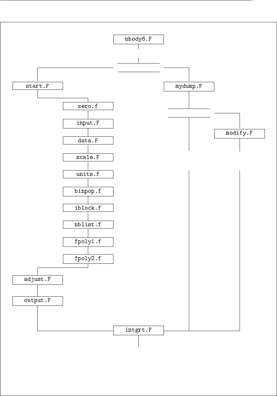
58 Flow chart
read init. parameters
KSTART = 1 ?
yes
new run
?
no restart
?
KSTART > 2 ?
no
restart without
any changes
?
yes
restart with
some small changes
-
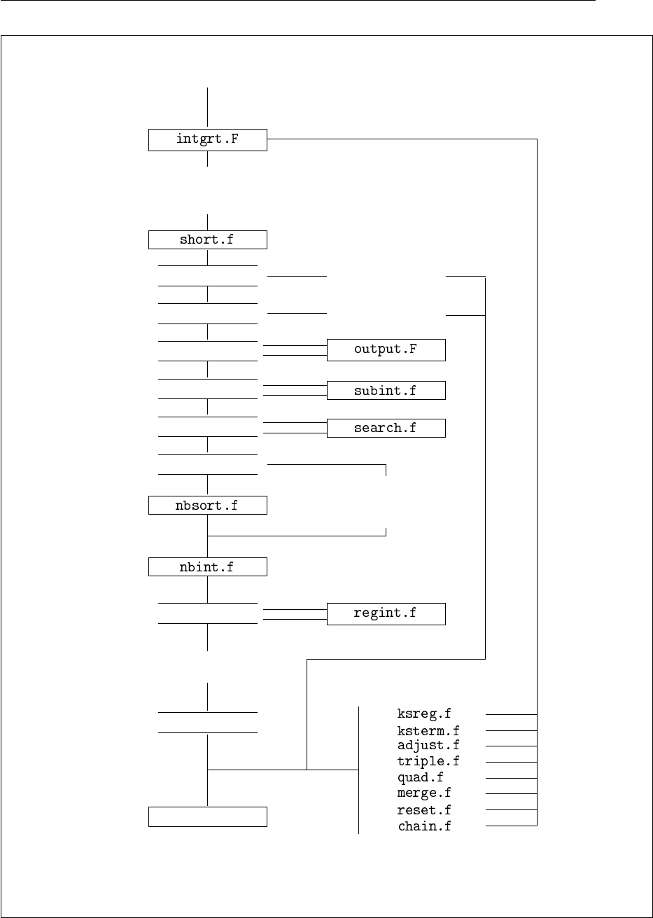
Flow chart 59
Determine group of particles
due to be advanced;
create list: NXTLST(I)
create a sublist of
shortest times steps
IKS > 0 ? -
yes set IPHASE = 1
?
no
TIME > TADJ ? -
yes set IPHASE = 3
?
no
TIME > TNEXT ? -
yes
?
no
TIME > TPREV ? -
yes
?
no
STEP(I)<DTMIN ? -
yes
?
no
NXTLEN > 10 ? yes
?
no
partial
predict.
prediction of all
particles not
to be corrected
treg+dtreg=TIME? -
yes
no
Update new positions
and velocities
Termination ?
yes
STOP
no -
Continue acc. to IPHASE:
1:
2:
3:
4:
5:
6:
7:
8:
?

60 References
Bibliography
[1] Aarseth S.J. (1963):Mon. Not. Roy. Astron. Soc. 126, p223
[2] Aarseth S.J. (1985): “Direct methods for N–body simulations”, in: Multiple Time Scales,
Brackbill J. & Cohen B. (eds.), Ch. 12, p377
[3] Aarseth S.J. (1993): “Direct methods for N–body simulations”, in: Galactic Dynamics
and N–body simulations, Contopoulos G. et. al. (eds.), Symposium in Thessaloniki, Greece
[4] Aarseth S.J. (1999a):Publ. Astron. Soc. Pac. 111, p1333
[5] Aarseth S.J. (1999b):Celect. Mech. Dyn. Astron. 73, p127
[6] Aarseth S.J. (2003): “Gravitational N–Body Simulations, Tools and Algorithms”, Cam-
bridge University Press, 430 pages, ISBN 0521432723
[7] Aarseth S.J., Hénon M., Wielen R. (1974):Astron. Astrophys. 37, p183
[8] Aarseth S.J., Zare . (1974):Celest. Mech. 10, p185
[9] Ahmad A. & Cohen L. (1973):J. Comput. Phys. 12, p389
[10] Cohn H. (1980):ApJ 242, p765
[11] Dorband E.N., Hemsendorf M., Merritt D. (2003):J. Comput. Phys. 185, p484–511
[12] Heggie D.C. & Mathieu R.D. (1986): “Standardised units and time scales”, in: The Use of
Supercomputers in Stellar Dynamics, Hut P. & McMillan S. (eds.), p233
[13] Hénon M. (1971):Astrophys. Space Sci. 14, p151
[14] Kustaanheimo P. & Stiefel E.L. (1965):J. für Reine Angewandte Mathematik 218, p204
[15] Makino J. (1991a):Publ. Astron. Soc. Japan 43, p859
[16] Makino J. (1991b):ApJ 369, p200
[17] Makino J. & Aarseth S.J. (1992):Publ. Astron. Soc. Japan 44, p141
[18] Makino J. & Hut, P. (1988):ApJ Suppl. 68, p833
[19] Makino J., Taiji M., Ebisuzaki T., Sugimoto D. (1997):ApJ 480, p432–446
[20] Mikkola S. (1997): “Numerical Treatment of Small Stellar Systems with Binaries”, in:
Visual Double Stars: Formation, Dynamics and Evolutionary Tracks, Docobo J.A., Elipe
A., & McAlister H. (eds.), p269
[21] Mikkola S. & Aarseth, S.J. (1990):Celest. Mech. Dyn. Ast. 47, p375
[22] Mikkola S. & Aarseth, S.J. (1993):Celest. Mech. Dyn. Ast. 57, p439
[23] Mikkola S. & Aarseth, S.J. (1996):Celest. Mech. Dyn. Ast. 64, p197
[24] Mikkola S. & Aarseth, S.J. (1998):New Astronomy 3, p309

References 61
[25] Neutsch W. & Scherer K. (1992): “Celestial Mechanics”, Bibliographisches Institut, 484
pages, ISBN 3411154810
[26] Spitzer L. jr. (1987):Dynamical Evolution of Globular Clusters, Princeton University
Press, New Jersey, USA
[27] Spurzem R. (1994): “Gravothermal Oscillations”, in: Ergodic Concepts in Stellar Dynam-
ics, Gurzadyan V.G. & Pfenniger D. (eds.), p170
[28] Spurzem R. (1999):J. Comput. Appl. Math. 109, p407
[29] von Hoerner S. (1960):Zeitschrift f. Astrophysik 50, p184–214
[30] von Hoerner S. (1963):Zeitschrift f. Astrophysik 57, p47–82
