The Neo4j Cypher Manual V3.5 3.5
neo4j-cypher-manual-3.5
User Manual:
Open the PDF directly: View PDF ![]() .
.
Page Count: 434 [warning: Documents this large are best viewed by clicking the View PDF Link!]

The Neo4j Cypher Manual v3.5
Table of Contents
1. Introduction . . . . . . . . . . . . . . . . . . . . . . . . . . . . . . . . . . . . . . . . . . . . . . . . . . . . . . . . . . . . . . . . . . . . . . . . . . . Ê2
2. Syntax. . . . . . . . . . . . . . . . . . . . . . . . . . . . . . . . . . . . . . . . . . . . . . . . . . . . . . . . . . . . . . . . . . . . . . . . . . . . . . . . . Ê7
3. Clauses. . . . . . . . . . . . . . . . . . . . . . . . . . . . . . . . . . . . . . . . . . . . . . . . . . . . . . . . . . . . . . . . . . . . . . . . . . . . . . . Ê74
4. Functions . . . . . . . . . . . . . . . . . . . . . . . . . . . . . . . . . . . . . . . . . . . . . . . . . . . . . . . . . . . . . . . . . . . . . . . . . . . . Ê153
5. Schema . . . . . . . . . . . . . . . . . . . . . . . . . . . . . . . . . . . . . . . . . . . . . . . . . . . . . . . . . . . . . . . . . . . . . . . . . . . . . Ê283
6. Query tuning . . . . . . . . . . . . . . . . . . . . . . . . . . . . . . . . . . . . . . . . . . . . . . . . . . . . . . . . . . . . . . . . . . . . . . . . . Ê313
7. Execution plans . . . . . . . . . . . . . . . . . . . . . . . . . . . . . . . . . . . . . . . . . . . . . . . . . . . . . . . . . . . . . . . . . . . . . . Ê338
8. Deprecations, additions and compatibility . . . . . . . . . . . . . . . . . . . . . . . . . . . . . . . . . . . . . . . . . . . . . . . Ê418
9. Glossary of keywords . . . . . . . . . . . . . . . . . . . . . . . . . . . . . . . . . . . . . . . . . . . . . . . . . . . . . . . . . . . . . . . . . Ê422

© 2018 Neo4j, Inc.
License: Creative Commons 4.0
This is the Cypher manual for Neo4j version 3.5, authored by the Neo4j Team.
This manual covers the following areas:
•Introduction — Introducing the Cypher query language.
•Syntax — Learn Cypher query syntax.
•Clauses — Reference of Cypher query clauses.
•Functions — Reference of Cypher query functions.
•Schema — Working with indexes and constraints in Cypher.
•Query tuning — Learn to analyze queries and tune them for performance.
•Execution plans — Cypher execution plans and operators.
•Deprecations, additions and compatibility — An overview of language
developments across versions.
•Glossary of keywords — A glossary of Cypher keywords, with links to other
parts of the Cypher manual.
Who should read this?
This manual is written for the developer of a Neo4j client application.
1
Chapter 1. Introduction
This section provides an introduction to the Cypher query language.
1.1. What is Cypher?
Cypher is a declarative graph query language that allows for expressive and efficient querying and
updating of the graph. It is designed to be suitable for both developers and operations professionals.
Cypher is designed to be simple, yet powerful; highly complicated database queries can be easily
expressed, enabling you to focus on your domain, instead of getting lost in database access.
Cypher is inspired by a number of different approaches and builds on established practices for
expressive querying. Many of the keywords, such as WHERE and ORDER BY, are inspired by SQL
(http://en.wikipedia.org/wiki/SQL). Pattern matching borrows expression approaches from SPARQL
(http://en.wikipedia.org/wiki/SPARQL). Some of the list semantics are borrowed from languages such as
Haskell and Python. Cypher’s constructs, based on English prose and neat iconography, make queries
easy both to write, and to read.
Structure
Cypher borrows its structure from SQL — queries are built up using various clauses.
Clauses are chained together, and they feed intermediate result sets between each other. For
example, the matching variables from one MATCH clause will be the context that the next clause exists
in.
The query language is comprised of several distinct clauses. You can read more details about them
later in the manual.
Here are a few clauses used to read from the graph:
•MATCH: The graph pattern to match. This is the most common way to get data from the graph.
•WHERE: Not a clause in its own right, but rather part of MATCH, OPTIONAL MATCH and WITH. Adds
constraints to a pattern, or filters the intermediate result passing through WITH.
•RETURN: What to return.
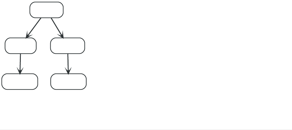
Let’s see MATCH and RETURN in action.
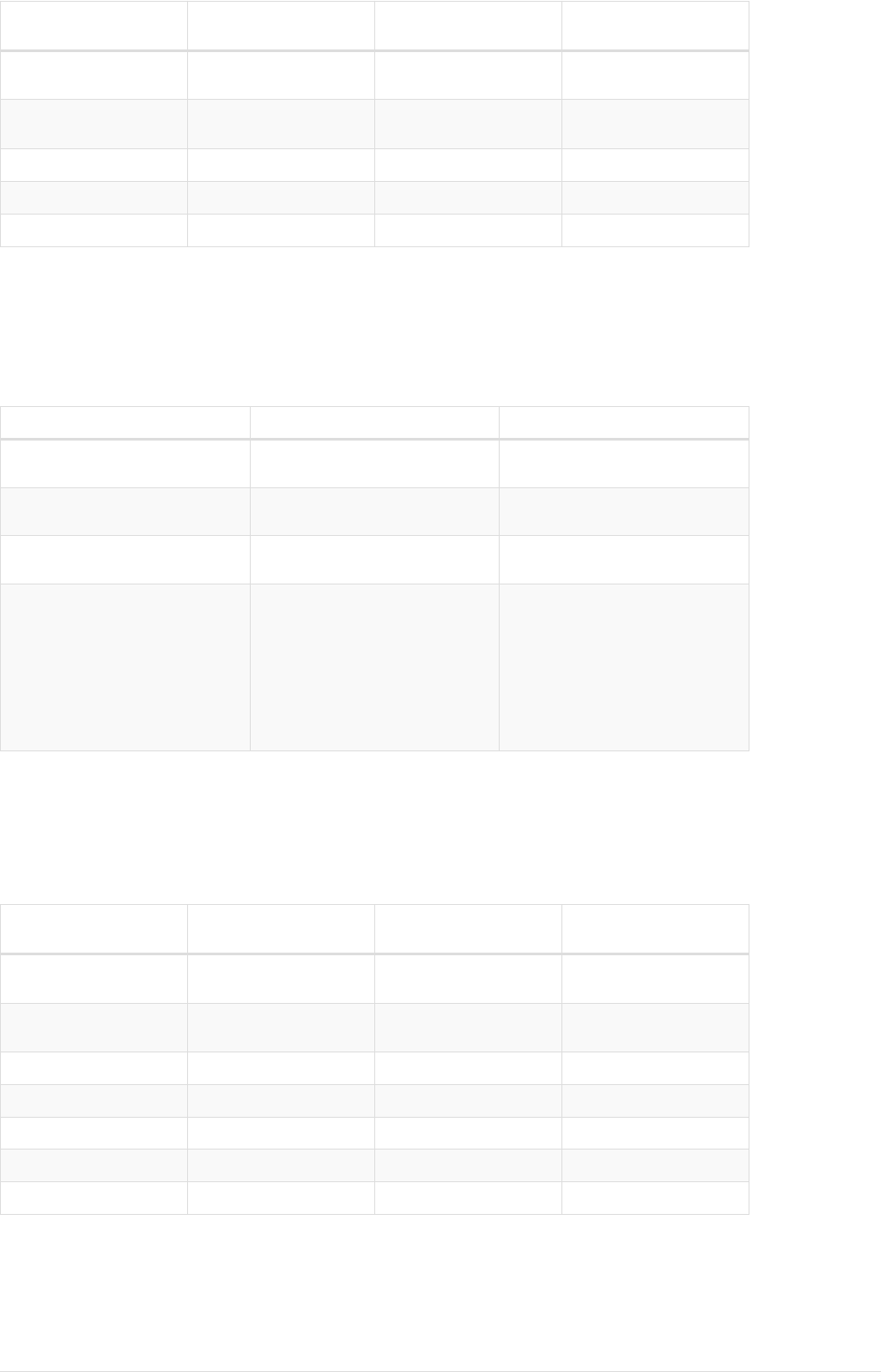
Imagine an example graph like the following one:
name = 'Joe'
name = 'Steve'
friend
name = 'John'
friend
name = 'Sara'
friend
name = 'Maria'
friend
Figure 1. Example Graph
For example, here is a query which finds a user called 'John' and 'John’s' friends (though not his direct
2

friends) before returning both 'John' and any friends-of-friends that are found.
MATCH (john {name: 'John'})-[:friend]->()-[:friend]->(fof)
RETURN john.name, fof.name
Resulting in:
+----------------------+
| john.name | fof.name |
+----------------------+
| "John" | "Maria" |
| "John" | "Steve" |
+----------------------+
2 rows
Next up we will add filtering to set more parts in motion:
We take a list of user names and find all nodes with names from this list, match their friends and
return only those followed users who have a 'name' property starting with 'S'.
MATCH (user)-[:friend]->(follower)
WHERE user.name IN ['Joe', 'John', 'Sara', 'Maria', 'Steve'] AND follower.name =~ 'S.*'
RETURN user.name, follower.name
Resulting in:
+---------------------------+
| user.name | follower.name |
+---------------------------+
| "Joe" | "Steve" |
| "John" | "Sara" |
+---------------------------+
2 rows
And here are examples of clauses that are used to update the graph:
•CREATE (and DELETE): Create (and delete) nodes and relationships.
•SET (and REMOVE): Set values to properties and add labels on nodes using SET and use REMOVE to
remove them.
•MERGE: Match existing or create new nodes and patterns. This is especially useful together with
unique constraints.
1.2. Querying and updating the graph
Cypher can be used for both querying and updating your graph.
1.2.1. The structure of update queries
A Cypher query part can’t both match and update the graph at the same time.
Every part can either read and match on the graph, or make updates on it.
If you read from the graph and then update the graph, your query implicitly has two parts — the
reading is the first part, and the writing is the second part.
If your query only performs reads, Cypher will be lazy and not actually match the pattern until you ask
for the results. In an updating query, the semantics are that all the reading will be done before any
3

writing actually happens.
The only pattern where the query parts are implicit is when you first read and then write — any other
order and you have to be explicit about your query parts. The parts are separated using the WITH
statement. WITH is like an event horizon — it’s a barrier between a plan and the finished execution of
that plan.
When you want to filter using aggregated data, you have to chain together two reading query
parts — the first one does the aggregating, and the second filters on the results coming from the first
one.
MATCH (n {name: 'John'})-[:FRIEND]-(friend)
WITH n, count(friend) AS friendsCount
WHERE friendsCount > 3
RETURN n, friendsCount
Using WITH, you specify how you want the aggregation to happen, and that the aggregation has to be
finished before Cypher can start filtering.
Here’s an example of updating the graph, writing the aggregated data to the graph:
MATCH (n {name: 'John'})-[:FRIEND]-(friend)
WITH n, count(friend) AS friendsCount
SET n.friendsCount = friendsCount
RETURN n.friendsCount
You can chain together as many query parts as the available memory permits.
1.2.2. Returning data
Any query can return data. If your query only reads, it has to return data — it serves no purpose if it
doesn’t, and it is not a valid Cypher query. Queries that update the graph don’t have to return
anything, but they can.
After all the parts of the query comes one final RETURN clause. RETURN is not part of any query part — it
is a period symbol at the end of a query. The RETURN clause has three sub-clauses that come with it:
SKIP/LIMIT and ORDER BY.
If you return nodes or relationships from a query that has just deleted them — beware, you are
holding a pointer that is no longer valid.
1.3. Transactions
Any query that updates the graph will run in a transaction. An updating query will always either fully
succeed, or not succeed at all.
Cypher will either create a new transaction or run inside an existing one:
•If no transaction exists in the running context Cypher will create one and commit it once the query
finishes.
•In case there already exists a transaction in the running context, the query will run inside it, and
nothing will be persisted to disk until that transaction is successfully committed.
This can be used to have multiple queries be committed as a single transaction:
1. Open a transaction,
2. Run multiple updating Cypher queries.
4
3. Commit all of them in one go.
Note that a query will hold the changes in memory until the whole query has finished executing. A
large query will consequently use large amounts of memory. For memory configuration in Neo4j, see
the Neo4j Operations Manual.
For using transactions with a Neo4j driver, see the Neo4j Driver manual. For using transactions over
the HTTP API, see the HTTP API documentation.
When writing procedures or using Neo4j embedded, remember that all iterators returned from an
execution result should be either fully exhausted or closed. This ensures that the resources bound to
them are properly released.
1.4. Uniqueness
While pattern matching, Neo4j makes sure to not include matches where the same graph relationship
is found multiple times in a single pattern. In most use cases, this is a sensible thing to do.
Example: looking for a user’s friends of friends should not return said user.
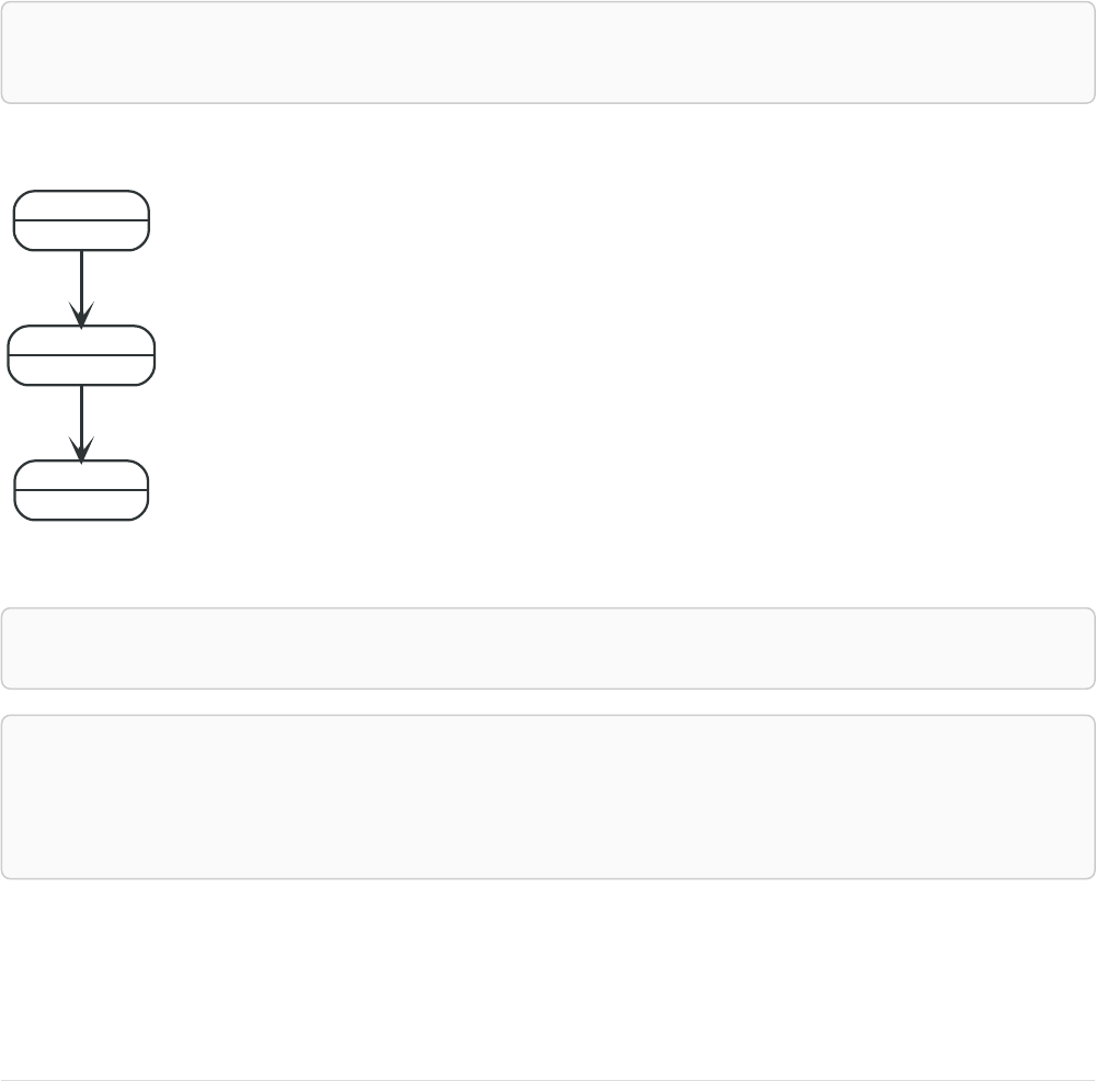
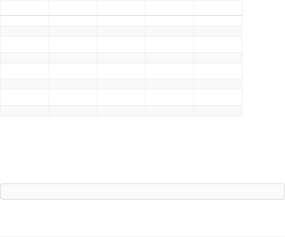
Let’s create a few nodes and relationships:
CREATE (adam:User { name: 'Adam' }),(pernilla:User { name: 'Pernilla' }),(david:User { name: 'David'
Ê }),
Ê (adam)-[:FRIEND]->(pernilla),(pernilla)-[:FRIEND]->(david)
Which gives us the following graph:
User
name = 'Adam'
User
name = 'Pernilla'
FRIEND
User
name = 'David'
FRIEND
Now let’s look for friends of friends of Adam:
MATCH (user:User { name: 'Adam' })-[r1:FRIEND]-()-[r2:FRIEND]-(friend_of_a_friend)
RETURN friend_of_a_friend.name AS fofName
+---------+
| fofName |
+---------+
| "David" |
+---------+
1 row
In this query, Cypher makes sure to not return matches where the pattern relationships r1 and r2
point to the same graph relationship.
This is however not always desired. If the query should return the user, it is possible to spread the
5

matching over multiple MATCH clauses, like so:
MATCH (user:User { name: 'Adam' })-[r1:FRIEND]-(friend)
MATCH (friend)-[r2:FRIEND]-(friend_of_a_friend)
RETURN friend_of_a_friend.name AS fofName
+---------+
| fofName |
+---------+
| "David" |
| "Adam" |
+---------+
2 rows
Note that while the following query looks similar to the previous one, it is actually equivalent to the
one before.
MATCH (user:User { name: 'Adam' })-[r1:FRIEND]-(friend),(friend)-[r2:FRIEND]-(friend_of_a_friend)
RETURN friend_of_a_friend.name AS fofName
Here, the MATCH clause has a single pattern with two paths, while the previous query has two distinct
patterns.
+---------+
| fofName |
+---------+
| "David" |
+---------+
1 row
6

Chapter 2. Syntax
This section describes the syntax of the Cypher query language.
•Values and types
•Naming rules and recommendations
•Expressions
•Expressions in general
•Note on string literals
•CASE Expressions
•Variables
•Reserved keywords
•Parameters
•String literal
•Regular expression
•Case-sensitive string pattern matching
•Create node with properties
•Create multiple nodes with properties
•Setting all properties on a node
•SKIP and LIMIT
•Node id
•Multiple node ids
•Calling procedures
•Index value (explicit indexes)
•Index query (explicit indexes)
•Operators
•Operators at a glance
•Aggregation operators
•Mathematical operators
•Comparison operators
•Boolean operators
•String operators
•Temporal operators
•List operators
•Property operators
•Equality and comparison of values
•Ordering and comparison of values
•Chaining comparison operations
•Comments
7

•Patterns
•Patterns for nodes
•Patterns for related nodes
•Patterns for labels
•Specifying properties
•Patterns for relationships
•Variable-length pattern matching
•Assigning to path variables
•Temporal (Date/Time) values
•Introduction
•Time zones
•Temporal instants
•Specifying temporal instants
•Specifying dates
•Specifying times
•Specifying time zones
•Examples
•Accessing components of temporal instants
•Durations
•Specifying durations
•Examples
•Accessing components of durations
•Examples
•Temporal indexing
•Spatial values
•Introduction
•Coordinate Reference Systems
•Geographic coordinate reference systems
•Cartesian coordinate reference systems
•Spatial instants
•Creating points
•Accessing components of points
•Spatial index
•Lists
•Lists in general
•List comprehension
•Pattern comprehension
8

•Maps
•Literal maps
•Map projection
•Working with null
•Introduction to null in Cypher
•Logical operations with null
•The [] operator and null
•The IN operator and null
•Expressions that return null
2.1. Values and types
Cypher provides first class support for a number of data types.
These fall into several categories which will be described in detail in the following subsections:
•Property types
•Structural types
•Composite types
2.1.1. Property types
☑Can be returned from Cypher queries
☑Can be used as parameters
☑Can be stored as properties
☑Can be constructed with Cypher literals
Property types comprise:
•Number, an abstract type, which has the subtypes Integer and Float
•String
•Boolean
•The spatial type Point
•Temporal types: Date, Time, LocalTime, DateTime, LocalDateTime and Duration
The adjective numeric, when used in the context of describing Cypher functions or expressions,
indicates that any type of Number applies (Integer or Float).
Homogeneous lists of simple types can also be stored as properties, although lists in general (see
Composite types) cannot be stored.
Cypher also provides pass-through support for byte arrays, which can be stored as property values.
Byte arrays are not considered a first class data type by Cypher, so do not have a literal
representation.
9

Sorting of special characters
Strings that contain characters that do not belong to the Basic Multilingual Plane
(https://en.wikipedia.org/wiki/Plane_(Unicode)#Basic_Multilingual_Plane) (BMP) can have
inconsistent or non-deterministic ordering in Neo4j. BMP is a subset of all
characters defined in Unicode. Expressed simply, it contains all common characters
from all common languages.
The most significant characters not in BMP are those belonging to the
Supplementary Multilingual Plane
(https://en.wikipedia.org/wiki/Plane_(Unicode)#Supplementary_Multilingual_Plane) or the
Supplementary Ideographic Plane
(https://en.wikipedia.org/wiki/Plane_(Unicode)#Supplementary_Ideographic_Plane). Examples
are:
•Historic scripts and symbols and notation used within certain fields such as:
Egyptian hieroglyphs, modern musical notation, mathematical alphanumerics.
•Emojis and other pictographic sets.
•Game symbols for playing cards, Mah Jongg, and dominoes.
•CJK Ideograph that were not included in earlier character encoding standards.
2.1.2. Structural types
☑Can be returned from Cypher queries
☐Cannot be used as parameters
☐Cannot be stored as properties
☐Cannot be constructed with Cypher literals
Structural types comprise:
•Nodes, comprising:
•Id
•Label(s)
•Map (of properties)
•Relationships, comprising:
•Id
•Type
•Map (of properties)
•Id of the start and end nodes
•Paths
•An alternating sequence of nodes and relationships
Nodes, relationships, and paths are returned as a result of pattern matching.
Labels are not values but are a form of pattern syntax.
10

2.1.3. Composite types
☑Can be returned from Cypher queries
☑Can be used as parameters
☐Cannot be stored as properties
☑Can be constructed with Cypher literals
Composite types comprise:
•Lists are heterogeneous, ordered collections of values, each of which has any property, structural
or composite type.
•Maps are heterogeneous, unordered collections of (key, value) pairs, where:
•the key is a String
•the value has any property, structural or composite type
Composite values can also contain null.
Special care must be taken when using null (see Working with null).
2.2. Naming rules and recommendations
We describe here rules and recommendations for the naming of node labels, relationship types,
property names and variables.
2.2.1. Naming rules
•Must begin with an alphabetic letter.
•This includes "non-English" characters, such as å, ä, ö, ü etc.
•If a leading non-alphabetic character is required, use backticks for escaping; e.g. `^n`.
•Can contain numbers, but not as the first character.
•To illustrate, 1first is not allowed, whereas first1 is allowed.
•If a leading numeric character is required, use backticks for escaping; e.g. `1first`.
•Cannot contain symbols.
•An exception to this rule is using underscore, as given by my_variable.
•An ostensible exception to this rule is using $ as the first character to denote a parameter, as
given by $myParam.
•If a leading symbolic character is required, use backticks for escaping; e.g. `$$n`.
•Can be very long, up to 65535 (2^16 - 1) or 65534 characters, depending on the version of Neo4j.
•Are case-sensitive.
•Thus, :PERSON, :Person and :person are three different labels, and n and N are two different
variables.
•Whitespace characters:
•Leading and trailing whitespace characters will be removed automatically. For example, MATCH
11

( a ) RETURN a is equivalent to MATCH (a) RETURN a.
•If spaces are required within a name, use backticks for escaping; e.g. `my variable has
spaces`.
2.2.2. Scoping and namespace rules
•Node labels, relationship types and property names may re-use names.
•The following query — with a for the label, type and property name — is valid: CREATE (a:a {a:
'a'})-[r:a]→(b:a {a: 'a'}).
•Variables for nodes and relationships must not re-use names within the same query scope.
•The following query is not valid as the node and relationship both have the name a: CREATE
(a)-[a]→(b).
2.2.3. Recommendations
Here are the naming conventions we recommend using:
Node labels Camel case, beginning with an upper-
case character
:VehicleOwner rather than
:vehice_owner etc.
Relationship types Upper case, using underscore to
separate words
:OWNS_VEHICLE rather than
:ownsVehicle etc
2.3. Expressions
•Expressions in general
•Note on string literals
•CASE expressions
•Simple CASE form: comparing an expression against multiple values
•Generic CASE form: allowing for multiple conditionals to be expressed
•Distinguishing between when to use the simple and generic CASE forms
2.3.1. Expressions in general
Most expressions in Cypher evaluate to null if any of their inner expressions are
null. Notable exceptions are the operators IS NULL and IS NOT NULL.
An expression in Cypher can be:
•A decimal (integer or double) literal: 13, -40000, 3.14, 6.022E23.
•A hexadecimal integer literal (starting with 0x): 0x13zf, 0xFC3A9, -0x66eff.
•An octal integer literal (starting with 0): 01372, 02127, -05671.
•A string literal: 'Hello', "World".
•A boolean literal: true, false, TRUE, FALSE.
•A variable: n, x, rel, myFancyVariable, `A name with weird stuff in it[]!`.
•A property: n.prop, x.prop, rel.thisProperty, myFancyVariable.`(weird property name)`.
12

•A dynamic property: n["prop"], rel[n.city + n.zip], map[coll[0]].
•A parameter: $param, $0
•A list of expressions: ['a', 'b'], [1, 2, 3], ['a', 2, n.property, $param], [ ].
•A function call: length(p), nodes(p).
•An aggregate function: avg(x.prop), count(*).
•A path-pattern: (a)-->()<--(b).
•An operator application: 1 + 2 and 3 < 4.
•A predicate expression is an expression that returns true or false: a.prop = 'Hello', length(p) >
10, exists(a.name).
•A regular expression: a.name =~ 'Tim.*'
•A case-sensitive string matching expression: a.surname STARTS WITH 'Sven', a.surname ENDS WITH
'son' or a.surname CONTAINS 'son'
•A CASE expression.
2.3.2. Note on string literals
String literals can contain the following escape sequences:
Escape sequence Character
\t Tab
\b Backspace
\n Newline
\r Carriage return
\f Form feed
\' Single quote
\" Double quote
\\ Backslash
\uxxxx Unicode UTF-16 code point (4 hex
digits must follow the \u)
\Uxxxxxxxx Unicode UTF-32 code point (8 hex
digits must follow the \U)
2.3.3. CASE expressions
Generic conditional expressions may be expressed using the well-known CASE construct. Two variants
of CASE exist within Cypher: the simple form, which allows an expression to be compared against
multiple values, and the generic form, which allows multiple conditional statements to be expressed.
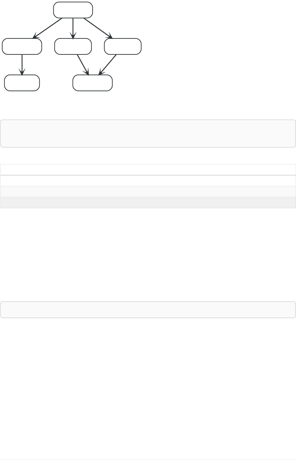
The following graph is used for the examples below:
13

A
name = 'Alice'
eyes = 'brown'
age = 38
C
name = 'Charlie'
eyes = 'green'
age = 53
KNOWS
B
name = 'Bob'
eyes = 'blue'
age = 25
KNOWS
D
name = 'Daniel'
eyes = 'brown'
KNOWS
E
array = ['one', 'two', 'three']
name = 'Eskil'
eyes = 'blue'
age = 41
MARRIEDKNOWS
Figure 2. Graph
Simple CASE form: comparing an expression against multiple values
The expression is calculated, and compared in order with the WHEN clauses until a match is found. If no
match is found, the expression in the ELSE clause is returned. However, if there is no ELSE case and no
match is found, null will be returned.
Syntax:
CASE test
ÊWHEN value THEN result
Ê [WHEN ...]
Ê [ELSE default]
END
Arguments:
Name Description
test A valid expression.
value An expression whose result will be compared to test.
result This is the expression returned as output if value matches
test.
default If no match is found, default is returned.
Query
MATCH (n)
RETURN
CASE n.eyes
WHEN 'blue'
THEN 1
WHEN 'brown'
THEN 2
ELSE 3 END AS result
Table 1. Result
result
2
1
14

result
3
2
1
5 rows
Generic CASE form: allowing for multiple conditionals to be expressed
The predicates are evaluated in order until a true value is found, and the result value is used. If no
match is found, the expression in the ELSE clause is returned. However, if there is no ELSE case and no
match is found, null will be returned.
Syntax:
CASE
WHEN predicate THEN result
Ê [WHEN ...]
Ê [ELSE default]
END
Arguments:
Name Description
predicate A predicate that is tested to find a valid alternative.
result This is the expression returned as output if predicate
evaluates to true.
default If no match is found, default is returned.
Query
MATCH (n)
RETURN
CASE
WHEN n.eyes = 'blue'
THEN 1
WHEN n.age < 40
THEN 2
ELSE 3 END AS result
Table 2. Result
result
2
1
3
3
1
5 rows
Distinguishing between when to use the simple and generic CASE forms
Owing to the close similarity between the syntax of the two forms, sometimes it may not be clear at
the outset as to which form to use. We illustrate this scenario by means of the following query, in
15

which there is an expectation that age_10_years_ago is -1 if n.age is null:
Query
MATCH (n)
RETURN n.name,
CASE n.age
WHEN n.age IS NULL THEN -1
ELSE n.age - 10 END AS age_10_years_ago
However, as this query is written using the simple CASE form, instead of age_10_years_ago being -1 for
the node named Daniel, it is null. This is because a comparison is made between n.age and n.age IS
NULL. As n.age IS NULL is a boolean value, and n.age is an integer value, the WHEN n.age IS NULL THEN
-1 branch is never taken. This results in the ELSE n.age - 10 branch being taken instead, returning
null.
Table 3. Result
n.name age_10_years_ago
"Alice" 28
"Bob" 15
"Charlie" 43
"Daniel" <null>
"Eskil" 31
5 rows
The corrected query, behaving as expected, is given by the following generic CASE form:
Query
MATCH (n)
RETURN n.name,
CASE
WHEN n.age IS NULL THEN -1
ELSE n.age - 10 END AS age_10_years_ago
We now see that the age_10_years_ago correctly returns -1 for the node named Daniel.
Table 4. Result
n.name age_10_years_ago
"Alice" 28
"Bob" 15
"Charlie" 43
"Daniel" -1
"Eskil" 31
5 rows
2.4. Variables
When you reference parts of a pattern or a query, you do so by naming them. The names you give the
different parts are called variables.
In this example:
16

MATCH (n)-->(b)
RETURN b
The variables are n and b.
Information regarding the naming of variables may be found here.
Variables are only visible in the same query part
Variables are not carried over to subsequent queries. If multiple query parts are
chained together using WITH, variables have to be listed in the WITH clause to be
carried over to the next part. For more information see WITH.
2.5. Reserved keywords
We provide here a listing of reserved words, grouped by the categories from which they are drawn, all
of which have a special meaning in Cypher. In addition to this, we list a number of words that are
reserved for future use.
These reserved words are not permitted to be used as identifiers in the following contexts:
•Variables
•Function names
•Parameters
If any reserved keyword is escaped — i.e. is encapsulated by backticks `, such as `AND` — it would
become a valid identifier in the above contexts.
2.5.1. Clauses
•CALL
•CREATE
•DELETE
•DETACH
•EXISTS
•FOREACH
•LOAD
•MATCH
•MERGE
•OPTIONAL
•REMOVE
•RETURN
•SET
•START
•UNION
•UNWIND
•WITH
17

2.5.2. Subclauses
•LIMIT
•ORDER
•SKIP
•WHERE
•YIELD
2.5.3. Modifiers
•ASC
•ASCENDING
•ASSERT
•BY
•CSV
•DESC
•DESCENDING
•ON
2.5.4. Expressions
•ALL
•CASE
•ELSE
•END
•THEN
•WHEN
2.5.5. Operators
•AND
•AS
•CONTAINS
•DISTINCT
•ENDS
•IN
•IS
•NOT
•OR
•STARTS
•XOR
18

2.5.6. Schema
•CONSTRAINT
•CREATE
•DROP
•EXISTS
•INDEX
•NODE
•KEY
•UNIQUE
2.5.7. Hints
•INDEX
•JOIN
•PERIODIC
•COMMIT
•SCAN
•USING
2.5.8. Literals
•false
•null
•true
2.5.9. Reserved for future use
•ADD
•DO
•FOR
•MANDATORY
•OF
•REQUIRE
•SCALAR
2.6. Parameters
•Introduction
•String literal
•Regular expression
•Case-sensitive string pattern matching
•Create node with properties
•Create multiple nodes with properties
19

•Setting all properties on a node
•SKIP and LIMIT
•Node id
•Multiple node ids
•Calling procedures
•Index value (explicit indexes)
•Index query (explicit indexes)
2.6.1. Introduction
Cypher supports querying with parameters. This means developers don’t have to resort to string
building to create a query. Additionally, parameters make caching of execution plans much easier for
Cypher, thus leading to faster query execution times.
Parameters can be used for:
•literals and expressions
•node and relationship ids
•for explicit indexes only: index values and queries
Parameters cannot be used for the following constructs, as these form part of the query structure that
is compiled into a query plan:
•property keys; so, MATCH (n) WHERE n.$param = 'something' is invalid
•relationship types
•labels
Parameters may consist of letters and numbers, and any combination of these, but cannot start with a
number or a currency symbol.
For details on using parameters via the Neo4j HTTP API, see the HTTP API documentation.
We provide below a comprehensive list of examples of parameter usage. In these examples,
parameters are given in JSON; the exact manner in which they are to be submitted depends upon the
driver being used.
It is recommended that the new parameter syntax $param is used, as the old syntax
{param} is deprecated and will be removed altogether in a later release.
2.6.2. String literal
Parameters
{
Ê "name" : "Johan"
}
Query
MATCH (n:Person)
WHERE n.name = $name
RETURN n
20

You can use parameters in this syntax as well:
Parameters
{
Ê "name" : "Johan"
}
Query
MATCH (n:Person { name: $name })
RETURN n
2.6.3. Regular expression
Parameters
{
Ê "regex" : ".*h.*"
}
Query
MATCH (n:Person)
WHERE n.name =~ $regex
RETURN n.name
2.6.4. Case-sensitive string pattern matching
Parameters
{
Ê "name" : "Michael"
}
Query
MATCH (n:Person)
WHERE n.name STARTS WITH $name
RETURN n.name
2.6.5. Create node with properties
Parameters
{
Ê "props" : {
Ê "name" : "Andy",
Ê "position" : "Developer"
Ê }
}
Query
CREATE ($props)
21

2.6.6. Create multiple nodes with properties
Parameters
{
Ê "props" : [ {
Ê "awesome" : true,
Ê "name" : "Andy",
Ê "position" : "Developer"
Ê }, {
Ê "children" : 3,
Ê "name" : "Michael",
Ê "position" : "Developer"
Ê } ]
}
Query
UNWIND $props AS properties
CREATE (n:Person)
SET n = properties
RETURN n
2.6.7. Setting all properties on a node
Note that this will replace all the current properties.
Parameters
{
Ê "props" : {
Ê "name" : "Andy",
Ê "position" : "Developer"
Ê }
}
Query
MATCH (n:Person)
WHERE n.name='Michaela'
SET n = $props
2.6.8. SKIP and LIMIT
Parameters
{
Ê "s" : 1,
Ê "l" : 1
}
Query
MATCH (n:Person)
RETURN n.name
SKIP $s
LIMIT $l
2.6.9. Node id
22

Parameters
{
Ê "id" : 0
}
Query
MATCH (n)
WHERE id(n)= $id
RETURN n.name
2.6.10. Multiple node ids
Parameters
{
Ê "ids" : [ 0, 1, 2 ]
}
Query
MATCH (n)
WHERE id(n) IN $ids
RETURN n.name
2.6.11. Calling procedures
Parameters
{
Ê "indexname" : ":Person(name)"
}
Query
CALL db.resampleIndex($indexname)
2.6.12. Index value (explicit indexes)
Parameters
{
Ê "value" : "Michaela"
}
Query
START n=node:people(name = $value)
RETURN n
2.6.13. Index query (explicit indexes)
23

Parameters
{
Ê "query" : "name:Bob"
}
Query
START n=node:people($query)
RETURN n
2.7. Operators
•Operators at a glance
•Aggregation operators
•Using the DISTINCT operator
•Property operators
•Statically accessing a property of a node or relationship using the . operator
•Filtering on a dynamically-computed property key using the [] operator
•Replacing all properties of a node or relationship using the = operator
•Mutating specific properties of a node or relationship using the += operator
•Mathematical operators
•Using the exponentiation operator ^
•Using the unary minus operator -
•Comparison operators
•Comparing two numbers
•Using STARTS WITH to filter names
•Boolean operators
•Using boolean operators to filter numbers
•String operators
•Using a regular expression with =~ to filter words
•Temporal operators
•Adding and subtracting a Duration to or from a temporal instant
•Adding and subtracting a Duration to or from another Duration
•Multiplying and dividing a Duration with or by a number
•Map operators
•Statically accessing the value of a nested map by key using the . operator"
•Dynamically accessing the value of a map by key using the [] operator and a parameter
•Using IN with [] on a nested list
•List operators
•Concatenating two lists using +
24

•Using IN to check if a number is in a list
•Using IN for more complex list membership operations
•Accessing elements in a list using the [] operator
•Dynamically accessing an element in a list using the [] operator and a parameter
•Equality and comparison of values
•Ordering and comparison of values
•Chaining comparison operations
2.7.1. Operators at a glance
Aggregation operators DISTINCT
Property operators . for static property access, [] for dynamic property
access, = for replacing all properties, += for mutating
specific properties
Mathematical operators +, -, *, /, %, ^
Comparison operators =, <>, <, >, <=, >=, IS NULL, IS NOT NULL
String-specific comparison operators STARTS WITH, ENDS WITH, CONTAINS
Boolean operators AND, OR, XOR, NOT
String operators + for concatenation, =~ for regex matching
Temporal operators + and - for operations between durations and temporal
instants/durations, * and / for operations between
durations and numbers
Map operators . for static value access by key, [] for dynamic value access
by key
List operators + for concatenation, IN to check existence of an element in
a list, [] for accessing element(s) dynamically
2.7.2. Aggregation operators
The aggregation operators comprise:
•remove duplicates values: DISTINCT
Using the DISTINCT operator
Retrieve the unique eye colors from Person nodes.
Query
CREATE (a:Person { name: 'Anne', eyeColor: 'blue' }),(b:Person { name: 'Bill', eyeColor: 'brown'
}),(c:Person { name: 'Carol', eyeColor: 'blue' })
WITH [a, b, c] AS ps
UNWIND ps AS p
RETURN DISTINCT p.eyeColor
Even though both 'Anne' and 'Carol' have blue eyes, 'blue' is only returned once.
Table 5. Result
p.eyeColor
"blue"
25

p.eyeColor
"brown"
2 rows
Nodes created: 3
Properties set: 6
Labels added: 3
DISTINCT is commonly used in conjunction with aggregating functions.
2.7.3. Property operators
The property operators pertain to a node or a relationship, and comprise:
•statically access the property of a node or relationship using the dot operator: .
•dynamically access the property of a node or relationship using the subscript operator: []
•property replacement = for replacing all properties of a node or relationship
•property mutation operator += for setting specific properties of a node or relationship
Statically accessing a property of a node or relationship using the . operator
Query
CREATE (a:Person { name: 'Jane', livesIn: 'London' }),(b:Person { name: 'Tom', livesIn: 'Copenhagen' })
WITH a, b
MATCH (p:Person)
RETURN p.name
Table 6. Result
p.name
"Jane"
"Tom"
2 rows
Nodes created: 2
Properties set: 4
Labels added: 2
Filtering on a dynamically-computed property key using the [] operator
Query
CREATE (a:Restaurant { name: 'Hungry Jo', rating_hygiene: 10, rating_food: 7 }),(b:Restaurant { name:
'Buttercup Tea Rooms', rating_hygiene: 5, rating_food: 6 }),(c1:Category { name: 'hygiene' }),(c2:Category
{ name: 'food' })
WITH a, b, c1, c2
MATCH (restaurant:Restaurant),(category:Category)
WHERE restaurant["rating_" + category.name]> 6
RETURN DISTINCT restaurant.name
Table 7. Result
restaurant.name
"Hungry Jo"
1 row
Nodes created: 4
Properties set: 8
Labels added: 4
26

See Basic usage for more details on dynamic property access.
The behavior of the [] operator with respect to null is detailed here.
Replacing all properties of a node or relationship using the = operator
Query
CREATE (a:Person { name: 'Jane', age: 20 })
WITH a
MATCH (p:Person { name: 'Jane' })
SET p = { name: 'Ellen', livesIn: 'London' }
RETURN p.name, p.age, p.livesIn
All the existing properties on the node are replaced by those provided in the map; i.e. the name
property is updated from Jane to Ellen, the age property is deleted, and the livesIn property is added.
Table 8. Result
p.name p.age p.livesIn
"Ellen" <null> "London"
1 row
Nodes created: 1
Properties set: 5
Labels added: 1
See Replace all properties using a map and = for more details on using the property replacement
operator =.
Mutating specific properties of a node or relationship using the += operator
Query
CREATE (a:Person { name: 'Jane', age: 20 })
WITH a
MATCH (p:Person { name: 'Jane' })
SET p += { name: 'Ellen', livesIn: 'London' }
RETURN p.name, p.age, p.livesIn
The properties on the node are updated as follows by those provided in the map: the name property is
updated from Jane to Ellen, the age property is left untouched, and the livesIn property is added.
Table 9. Result
p.name p.age p.livesIn
"Ellen" 20 "London"
1 row
Nodes created: 1
Properties set: 4
Labels added: 1
See Mutate specific properties using a map and += for more details on using the property mutation
operator +=.
2.7.4. Mathematical operators
The mathematical operators comprise:
27

•addition: +
•subtraction or unary minus: -
•multiplication: *
•division: /
•modulo division: %
•exponentiation: ^
Using the exponentiation operator ^
Query
WITH 2 AS number, 3 AS exponent
RETURN number ^ exponent AS result
Table 10. Result
result
8.0
1 row
Using the unary minus operator -
Query
WITH -3 AS a, 4 AS b
RETURN b - a AS result
Table 11. Result
result
7
1 row
2.7.5. Comparison operators
The comparison operators comprise:
•equality: =
•inequality: <>
•less than: <
•greater than: >
•less than or equal to: <=
•greater than or equal to: >=
•IS NULL
•IS NOT NULL
String-specific comparison operators comprise:
•STARTS WITH: perform case-sensitive prefix searching on strings
28

•ENDS WITH: perform case-sensitive suffix searching on strings
•CONTAINS: perform case-sensitive inclusion searching in strings
Comparing two numbers
Query
WITH 4 AS one, 3 AS two
RETURN one > two AS result
Table 12. Result
result
true
1 row
See Equality and comparison of values for more details on the behavior of comparison operators, and
Using ranges for more examples showing how these may be used.
Using STARTS WITH to filter names
Query
WITH ['John', 'Mark', 'Jonathan', 'Bill'] AS somenames
UNWIND somenames AS names
WITH names AS candidate
WHERE candidate STARTS WITH 'Jo'
RETURN candidate
Table 13. Result
candidate
"John"
"Jonathan"
2 rows
String matching contains more information regarding the string-specific comparison operators as well
as additional examples illustrating the usage thereof.
2.7.6. Boolean operators
The boolean operators — also known as logical operators — comprise:
•conjunction: AND
•disjunction: OR,
•exclusive disjunction: XOR
•negation: NOT
Here is the truth table for AND, OR, XOR and NOT.
a b a AND b a OR b a XOR b NOT a
false false false false false true
false null false null null true
29

a b a AND b a OR b a XOR b NOT a
false true false true true true
true false false true true false
true null null true null false
true true true true false false
null false false null null null
null null null null null null
null true null true null null
Using boolean operators to filter numbers
Query
WITH [2, 4, 7, 9, 12] AS numberlist
UNWIND numberlist AS number
WITH number
WHERE number = 4 OR (number > 6 AND number < 10)
RETURN number
Table 14. Result
number
4
7
9
3 rows
2.7.7. String operators
The string operators comprise:
•concatenating strings: +
•matching a regular expression: =~
Using a regular expression with =~ to filter words
Query
WITH ['mouse', 'chair', 'door', 'house'] AS wordlist
UNWIND wordlist AS word
WITH word
WHERE word =~ '.*ous.*'
RETURN word
Table 15. Result
word
"mouse"
"house"
2 rows
Further information and examples regarding the use of regular expressions in filtering can be found in
30

Regular expressions. In addition, refer to String-specific comparison operators comprise: for details on
string-specific comparison operators.
2.7.8. Temporal operators
Temporal operators comprise:
•adding a Duration to either a temporal instant or another Duration: +
•subtracting a Duration from either a temporal instant or another Duration: -
•multiplying a Duration with a number: *
•dividing a Duration by a number: /
The following table shows — for each combination of operation and operand type — the type of the
value returned from the application of each temporal operator:
Operator Left-hand operand Right-hand operand Type of result
+Temporal instant Duration The type of the temporal
instant
+Duration Temporal instant The type of the temporal
instant
-Temporal instant Duration The type of the temporal
instant
+Duration Duration Duration
-Duration Duration Duration
*Duration Number Duration
*Number Duration Duration
/Duration Number Duration
Adding and subtracting a Duration to or from a temporal instant
Query
WITH localdatetime({ year:1984, month:10, day:11, hour:12, minute:31, second:14 }) AS aDateTime,
duration({ years: 12, nanoseconds: 2 }) AS aDuration
RETURN aDateTime + aDuration, aDateTime - aDuration
Table 16. Result
aDateTime + aDuration aDateTime - aDuration
1996-10-11T12:31:14.000000002 1972-10-11T12:31:13.999999998
1 row
Components of a Duration that do not apply to the temporal instant are ignored. For example, when
adding a Duration to a Date, the hours, minutes, seconds and nanoseconds of the Duration are ignored
(Time behaves in an analogous manner):
Query
WITH date({ year:1984, month:10, day:11 }) AS aDate, duration({ years: 12, nanoseconds: 2 }) AS aDuration
RETURN aDate + aDuration, aDate - aDuration
Table 17. Result
31

aDate + aDuration aDate - aDuration
1996-10-11 1972-10-11
1 row
Adding two durations to a temporal instant is not an associative operation. This is because non-
existing dates are truncated to the nearest existing date:
Query
RETURN (date("2011-01-31")+ duration("P1M"))+ duration("P12M") AS date1, date("2011-01-
31")+(duration("P1M")+ duration("P12M")) AS date2
Table 18. Result
date1 date2
2012-02-28 2012-02-29
1 row
Adding and subtracting a Duration to or from another Duration
Query
WITH duration({ years: 12, months: 5, days: 14, hours: 16, minutes: 12, seconds: 70, nanoseconds: 1 }) AS
duration1, duration({ months:1, days: -14, hours: 16, minutes: -12, seconds: 70 }) AS duration2
RETURN duration1, duration2, duration1 + duration2, duration1 - duration2
Table 19. Result
duration1 duration2 duration1 + duration2 duration1 - duration2
P12Y5M14DT16H13M10.0000000
01S
P1M-14DT15H49M10S P12Y6MT32H2M20.000000001S P12Y4M28DT24M0.000000001S
1 row
Multiplying and dividing a Duration with or by a number
These operations are interpreted simply as component-wise operations with overflow to smaller units
based on an average length of units in the case of division (and multiplication with fractions).
Query
WITH duration({ days: 14, minutes: 12, seconds: 70, nanoseconds: 1 }) AS aDuration
RETURN aDuration, aDuration * 2, aDuration / 3
Table 20. Result
aDuration aDuration * 2 aDuration / 3
P14DT13M10.000000001S P28DT26M20.000000002S P4DT16H4M23.333333333S
1 row
2.7.9. Map operators
The map operators comprise:
•statically access the value of a map by key using the dot operator: .
32

•dynamically access the value of a map by key using the subscript operator: []
The behavior of the [] operator with respect to null is detailed in The [] operator
and null.
Statically accessing the value of a nested map by key using the . operator
Query
WITH { person: { name: 'Anne', age: 25 }} AS p
RETURN p.person.name
Table 21. Result
p.person.name
"Anne"
1 row
Dynamically accessing the value of a map by key using the [] operator and a
parameter
A parameter may be used to specify the key of the value to access:
Parameters
{
Ê "myKey" : "name"
}
Query
WITH { name: 'Anne', age: 25 } AS a
RETURN a[$myKey] AS result
Table 22. Result
result
"Anne"
1 row
More details on maps can be found in Maps.
2.7.10. List operators
The list operators comprise:
•concatenating lists l1 and l2: [l1] + [l2]
•checking if an element e exists in a list l: e IN [l]
•dynamically accessing an element(s) in a list using the subscript operator: []
The behavior of the IN and [] operators with respect to null is detailed here.
33

Concatenating two lists using +
Query
RETURN [1,2,3,4,5]+[6,7] AS myList
Table 23. Result
myList
[1,2,3,4,5,6,7]
1 row
Using IN to check if a number is in a list
Query
WITH [2, 3, 4, 5] AS numberlist
UNWIND numberlist AS number
WITH number
WHERE number IN [2, 3, 8]
RETURN number
Table 24. Result
number
2
3
2 rows
Using IN for more complex list membership operations
The general rule is that the IN operator will evaluate to true if the list given as the right-hand operand
contains an element which has the same type and contents (or value) as the left-hand operand. Lists
are only comparable to other lists, and elements of a list l are compared pairwise in ascending order
from the first element in l to the last element in l.
The following query checks whether or not the list [2, 1] is an element of the list [1, [2, 1], 3]:
Query
RETURN [2, 1] IN [1,[2, 1], 3] AS inList
The query evaluates to true as the right-hand list contains, as an element, the list [1, 2] which is of
the same type (a list) and contains the same contents (the numbers 2 and 1 in the given order) as the
left-hand operand. If the left-hand operator had been [1, 2] instead of [2, 1], the query would have
returned false.
Table 25. Result
inList
true
1 row
At first glance, the contents of the left-hand operand and the right-hand operand appear to be the
same in the following query:
34

Query
RETURN [1, 2] IN [1, 2] AS inList
However, IN evaluates to false as the right-hand operand does not contain an element that is of the
same type — i.e. a list — as the left-hand-operand.
Table 26. Result
inList
false
1 row
The following query can be used to ascertain whether or not a list llhs — obtained from, say, the
labels() function — contains at least one element that is also present in another list lrhs:
MATCH (n)
WHERE size([l IN labels(n) WHERE l IN ['Person', 'Employee'] | 1]) > 0
RETURN count(n)
As long as labels(n) returns either Person or Employee (or both), the query will return a value greater
than zero.
Accessing elements in a list using the [] operator
Query
WITH ['Anne', 'John', 'Bill', 'Diane', 'Eve'] AS names
RETURN names[1..3] AS result
The square brackets will extract the elements from the start index 1, and up to (but excluding) the end
index 3.
Table 27. Result
result
["John","Bill"]
1 row
Dynamically accessing an element in a list using the [] operator and a
parameter
A parameter may be used to specify the index of the element to access:
Parameters
{
Ê "myIndex" : 1
}
Query
WITH ['Anne', 'John', 'Bill', 'Diane', 'Eve'] AS names
RETURN names[$myIndex] AS result
35

Table 28. Result
result
"John"
1 row
Using IN with [] on a nested list
IN can be used in conjunction with [] to test whether an element exists in a nested list:
Parameters
{
Ê "myIndex" : 1
}
Query
WITH [[1, 2, 3]] AS l
RETURN 3 IN l[0] AS result
Table 29. Result
result
true
1 row
More details on lists can be found in Lists in general.
2.7.11. Equality and comparison of values
Equality
Cypher supports comparing values (see Values and types) by equality using the = and <> operators.
Values of the same type are only equal if they are the same identical value (e.g. 3 = 3 and "x" <>
"xy").
Maps are only equal if they map exactly the same keys to equal values and lists are only equal if they
contain the same sequence of equal values (e.g. [3, 4] = [1+2, 8/2]).
Values of different types are considered as equal according to the following rules:
•Paths are treated as lists of alternating nodes and relationships and are equal to all lists that
contain that very same sequence of nodes and relationships.
•Testing any value against null with both the = and the <> operators always is null. This includes
null = null and null <> null. The only way to reliably test if a value v is null is by using the
special v IS NULL, or v IS NOT NULL equality operators.
All other combinations of types of values cannot be compared with each other. Especially, nodes,
relationships, and literal maps are incomparable with each other.
It is an error to compare values that cannot be compared.
36

2.7.12. Ordering and comparison of values
The comparison operators <=, < (for ascending) and >=, > (for descending) are used to compare values
for ordering. The following points give some details on how the comparison is performed.
•Numerical values are compared for ordering using numerical order (e.g. 3 < 4 is true).
•The special value java.lang.Double.NaN is regarded as being larger than all other numbers.
•String values are compared for ordering using lexicographic order (e.g. "x" < "xy").
•Boolean values are compared for ordering such that false < true.
•Comparison of spatial values:
•Point values can only be compared within the same Coordinate Reference System
(CRS) — otherwise, the result will be null.
•For two points a and b within the same CRS, a is considered to be greater than b if a.x > b.x
and a.y > b.y (and a.z > b.z for 3D points).
•a is considered less than b if a.x < b.x and a.y < b.y (and a.z < b.z for 3D points).
•If none if the above is true, the points are considered incomparable and any comparison
operator between them will return null.
•Ordering of spatial values:
•ORDER BY requires all values to be orderable.
•Points are ordered after arrays and before temporal types.
•Points of different CRS are ordered by the CRS code (the value of SRID field). For the currently
supported set of Coordinate Reference Systems this means the order: 4326, 4979, 7302, 9157
•Points of the same CRS are ordered by each coordinate value in turn, x first, then y and finally
z.
•Note that this order is different to the order returned by the spatial index, which will be the
order of the space filling curve.
•Comparison of temporal values:
•Temporal instant values are comparable within the same type. An instant is considered less
than another instant if it occurs before that instant in time, and it is considered greater than if
it occurs after.
•Instant values that occur at the same point in time — but that have a different time zone — are
not considered equal, and must therefore be ordered in some predictable way. Cypher
prescribes that, after the primary order of point in time, instant values be ordered by effective
time zone offset, from west (negative offset from UTC) to east (positive offset from UTC). This
has the effect that times that represent the same point in time will be ordered with the time
with the earliest local time first. If two instant values represent the same point in time, and
have the same time zone offset, but a different named time zone (this is possible for DateTime
only, since Time only has an offset), these values are not considered equal, and ordered by the
time zone identifier, alphabetically, as its third ordering component.
•Duration values cannot be compared, since the length of a day, month or year is not known
without knowing which day, month or year it is. Since Duration values are not comparable, the
result of applying a comparison operator between two Duration values is null. If the type, point
in time, offset, and time zone name are all equal, then the values are equal, and any difference
in order is impossible to observe.
•Ordering of temporal values:
•ORDER BY requires all values to be orderable.
•Temporal instances are ordered after spatial instances and before strings.
37

•Comparable values should be ordered in the same order as implied by their comparison order.
•Temporal instant values are first ordered by type, and then by comparison order within the
type.
•Since no complete comparison order can be defined for Duration values, we define an order
for ORDER BY specifically for Duration:
•Duration values are ordered by normalising all components as if all years were 365.2425
days long (PT8765H49M12S), all months were 30.436875 (1/12 year) days long (PT730H29M06S),
and all days were 24 hours long [1: The 365.2425 days per year comes from the frequency
of leap years. A leap year occurs on a year with an ordinal number divisible by 4, that is not
divisible by 100, unless it divisible by 400. This means that over 400 years there are ((365 *
4 + 1) * 25 - 1) * 4 + 1 = 146097 days, which means an average of 365.2425 days per
year.].
•Comparing for ordering when one argument is null (e.g. null < 3 is null).
2.7.13. Chaining comparison operations
Comparisons can be chained arbitrarily, e.g., x < y <= z is equivalent to x < y AND y <= z.
Formally, if a, b, c, ..., y, z are expressions and op1, op2, ..., opN are comparison operators,
then a op1 b op2 c ... y opN z is equivalent to a op1 b and b op2 c and ... y opN z.
Note that a op1 b op2 c does not imply any kind of comparison between a and c, so that, e.g., x < y >
z is perfectly legal (although perhaps not elegant).
The example:
MATCH (n) WHERE 21 < n.age <= 30 RETURN n
is equivalent to
MATCH (n) WHERE 21 < n.age AND n.age <= 30 RETURN n
Thus it will match all nodes where the age is between 21 and 30.
This syntax extends to all equality and inequality comparisons, as well as extending to chains longer
than three.
For example:
a < b = c <= d <> e
Is equivalent to:
a < b AND b = c AND c <= d AND d <> e
For other comparison operators, see Comparison operators.
2.8. Comments
To add comments to your queries, use double slash. Examples:
38

MATCH (n) RETURN n //This is an end of line comment
MATCH (n)
//This is a whole line comment
RETURN n
MATCH (n) WHERE n.property = '//This is NOT a comment' RETURN n
2.9. Patterns
•Introduction
•Patterns for nodes
•Patterns for related nodes
•Patterns for labels
•Specifying properties
•Patterns for relationships
•Variable-length pattern matching
•Assigning to path variables
2.9.1. Introduction
Patterns and pattern-matching are at the very heart of Cypher, so being effective with Cypher requires
a good understanding of patterns.
Using patterns, you describe the shape of the data you’re looking for. For example, in the MATCH clause
you describe the shape with a pattern, and Cypher will figure out how to get that data for you.
The pattern describes the data using a form that is very similar to how one typically draws the shape
of property graph data on a whiteboard: usually as circles (representing nodes) and arrows between
them to represent relationships.
Patterns appear in multiple places in Cypher: in MATCH, CREATE and MERGE clauses, and in pattern
expressions. Each of these is described in more detail in:
•MATCH
•OPTIONAL MATCH
•CREATE
•MERGE
•Using path patterns in WHERE
2.9.2. Patterns for nodes
The very simplest 'shape' that can be described in a pattern is a node. A node is described using a
pair of parentheses, and is typically given a name. For example:
(a)
This simple pattern describes a single node, and names that node using the variable a.
39

2.9.3. Patterns for related nodes
A more powerful construct is a pattern that describes multiple nodes and relationships between
them. Cypher patterns describe relationships by employing an arrow between two nodes. For
example:
(a)-->(b)
This pattern describes a very simple data shape: two nodes, and a single relationship from one to the
other. In this example, the two nodes are both named as a and b respectively, and the relationship is
'directed': it goes from a to b.
This manner of describing nodes and relationships can be extended to cover an arbitrary number of
nodes and the relationships between them, for example:
(a)-->(b)<--(c)
Such a series of connected nodes and relationships is called a "path".
Note that the naming of the nodes in these patterns is only necessary should one need to refer to the
same node again, either later in the pattern or elsewhere in the Cypher query. If this is not necessary,
then the name may be omitted, as follows:
(a)-->()<--(c)
2.9.4. Patterns for labels
In addition to simply describing the shape of a node in the pattern, one can also describe attributes.
The most simple attribute that can be described in the pattern is a label that the node must have. For
example:
(a:User)-->(b)
One can also describe a node that has multiple labels:
(a:User:Admin)-->(b)
2.9.5. Specifying properties
Nodes and relationships are the fundamental structures in a graph. Neo4j uses properties on both of
these to allow for far richer models.
Properties can be expressed in patterns using a map-construct: curly brackets surrounding a number
of key-expression pairs, separated by commas. E.g. a node with two properties on it would look like:
(a {name: 'Andy', sport: 'Brazilian Ju-Jitsu'})
A relationship with expectations on it is given by:
(a)-[{blocked: false}]->(b)
40

When properties appear in patterns, they add an additional constraint to the shape of the data. In the
case of a CREATE clause, the properties will be set in the newly-created nodes and relationships. In the
case of a MERGE clause, the properties will be used as additional constraints on the shape any existing
data must have (the specified properties must exactly match any existing data in the graph). If no
matching data is found, then MERGE behaves like CREATE and the properties will be set in the newly
created nodes and relationships.
Note that patterns supplied to CREATE may use a single parameter to specify properties, e.g: CREATE
(node $paramName). This is not possible with patterns used in other clauses, as Cypher needs to know
the property names at the time the query is compiled, so that matching can be done effectively.
2.9.6. Patterns for relationships
The simplest way to describe a relationship is by using the arrow between two nodes, as in the
previous examples. Using this technique, you can describe that the relationship should exist and the
directionality of it. If you don’t care about the direction of the relationship, the arrow head can be
omitted, as exemplified by:
(a)--(b)
As with nodes, relationships may also be given names. In this case, a pair of square brackets is used to
break up the arrow and the variable is placed between. For example:
(a)-[r]->(b)
Much like labels on nodes, relationships can have types. To describe a relationship with a specific type,
you can specify this as follows:
(a)-[r:REL_TYPE]->(b)
Unlike labels, relationships can only have one type. But if we’d like to describe some data such that the
relationship could have any one of a set of types, then they can all be listed in the pattern, separating
them with the pipe symbol | like this:
(a)-[r:TYPE1|TYPE2]->(b)
Note that this form of pattern can only be used to describe existing data (ie. when using a pattern with
MATCH or as an expression). It will not work with CREATE or MERGE, since it’s not possible to create a
relationship with multiple types.
As with nodes, the name of the relationship can always be omitted, as exemplified by:
(a)-[:REL_TYPE]->(b)
2.9.7. Variable-length pattern matching
41

Variable length pattern matching in versions 2.1.x and earlier does not enforce
relationship uniqueness for patterns described within a single MATCH clause. This
means that a query such as the following: MATCH (a)-[r]->(b), p = (a)-[]->(c)
RETURN *, relationships(p) AS rs may include r as part of the rs set. This
behavior has changed in versions 2.2.0 and later, in such a way that r will
be excluded from the result set, as this better adheres to the rules of
relationship uniqueness as documented here Uniqueness. If you have a query
pattern that needs to retrace relationships rather than ignoring them as the
relationship uniqueness rules normally dictate, you can accomplish this using
multiple match clauses, as follows: MATCH (a)-[r]->(b) MATCH p = (a)-[]->(c)
RETURN *, relationships(p). This will work in all versions of Neo4j that support the
MATCH clause, namely 2.0.0 and later.
Rather than describing a long path using a sequence of many node and relationship descriptions in a
pattern, many relationships (and the intermediate nodes) can be described by specifying a length in
the relationship description of a pattern. For example:
(a)-[*2]->(b)
This describes a graph of three nodes and two relationship, all in one path (a path of length 2). This is
equivalent to:
(a)-->()-->(b)
A range of lengths can also be specified: such relationship patterns are called 'variable length
relationships'. For example:
(a)-[*3..5]->(b)
This is a minimum length of 3, and a maximum of 5. It describes a graph of either 4 nodes and 3
relationships, 5 nodes and 4 relationships or 6 nodes and 5 relationships, all connected together in a
single path.
Either bound can be omitted. For example, to describe paths of length 3 or more, use:
(a)-[*3..]->(b)
To describe paths of length 5 or less, use:
(a)-[*..5]->(b)
Both bounds can be omitted, allowing paths of any length to be described:
(a)-[*]->(b)
As a simple example, let’s take the graph and query below:
42
name = 'Anders'
name = 'Dilshad'
KNOWS
name = 'Cesar'
KNOWS
name = 'Becky'
KNOWS
name = 'Filipa'
KNOWS
name = 'George'
KNOWS KNOWS
Figure 3. Graph
Query
MATCH (me)-[:KNOWS*1..2]-(remote_friend)
WHERE me.name = 'Filipa'
RETURN remote_friend.name
Table 30. Result
remote_friend.name
"Dilshad"
"Anders"
2 rows
This query finds data in the graph which a shape that fits the pattern: specifically a node (with the
name property 'Filipa') and then the KNOWS related nodes, one or two hops away. This is a typical
example of finding first and second degree friends.
Note that variable length relationships cannot be used with CREATE and MERGE.
2.9.8. Assigning to path variables
As described above, a series of connected nodes and relationships is called a "path". Cypher allows
paths to be named using an identifer, as exemplified by:
p = (a)-[*3..5]->(b)
You can do this in MATCH, CREATE and MERGE, but not when using patterns as expressions.
2.10. Temporal (Date/Time) values
Cypher has built-in support for handling temporal values, and the underlying database
supports storing these temporal values as properties on nodes and relationships.
•Introduction
•Time zones
•Temporal instants
•Specifying temporal instants
•Specifying dates
43

•Specifying times
•Specifying time zones
•Examples
•Accessing components of temporal instants
•Durations
•Specifying durations
•Examples
•Accessing components of durations
•Examples
•Temporal indexing
Refer to Temporal functions - instant types for information regarding temporal
functions allowing for the creation and manipulation of temporal values.
Refer to Temporal operators for information regarding temporal operators.
Refer to Ordering and comparison of values for information regarding the
comparison and ordering of temporal values.
2.10.1. Introduction
The following table depicts the temporal value types and supported components:
Type Date support Time support Time zone support
Date X
Time X X
LocalTime X
DateTime X X X
LocalDateTime X X
Duration - - -
Date, Time, LocalTime, DateTime and LocalDateTime are temporal instant types. A temporal instant value
expresses a point in time with varying degrees of precision.
By contrast, Duration is not a temporal instant type. A Duration represents a temporal amount,
capturing the difference in time between two instants, and can be negative. Duration only captures
the amount of time between two instants, and thus does not encapsulate a start time and end time.
2.10.2. Time zones
Time zones are represented either as an offset from UTC, or as a logical identifier of a named time zone
(these are based on the IANA time zone database (https://www.iana.org/time-zones)). In either case the
time is stored as UTC internally, and the time zone offset is only applied when the time is presented.
This means that temporal instants can be ordered without taking time zone into account. If, however,
two times are identical in UTC, then they are ordered by timezone.
When creating a time using a named time zone, the offset from UTC is computed from the rules in the
time zone database to create a time instant in UTC, and to ensure the named time zone is a valid one.
44

It is possible for time zone rules to change in the IANA time zone database. For example, there could
be alterations to the rules for daylight savings time in a certain area. If this occurs after the creation of
a temporal instant, the presented time could differ from the originally-entered time, insofar as the
local timezone is concerned. However, the absolute time in UTC would remain the same.
There are three ways of specifying a time zone in Cypher:
•Specifying the offset from UTC in hours and minutes (ISO 8601 (https://en.wikipedia.org/wiki/ISO_8601))
•Specifying a named time zone
•Specifying both the offset and the time zone name (with the requirement that these match)
The named time zone form uses the rules of the IANA time zone database to manage daylight savings
time (DST).
The default time zone of the database can be configured using the configuration option
db.temporal.timezone. This configuration option influences the creation of temporal types for the
following functions:
•Getting the current date and time without specifying a time zone.
•Creating a temporal type from its components without specifying a time zone.
•Creating a temporal type by parsing a string without specifying a time zone.
•Creating a temporal type by combining or selecting values that do not have a time zone
component, and without specifying a time zone.
•Truncating a temporal value that does not have a time zone component, and without specifying a
time zone.
2.10.3. Temporal instants
Specifying temporal instants
A temporal instant consists of three parts; the date, the time, and the timezone. These parts may then
be combined to produce the various temporal value types. Literal characters are denoted in bold.
Temporal instant type Composition of parts
Date <date>
Time <time><timezone> or T<time><timezone>
LocalTime <time> or T<time>
DateTime*<date>T<time><timezone>
LocalDateTime*<date>T<time>
*When date and time are combined, date must be complete; i.e. fully identify a particular day.
Specifying dates
Component Format Description
Year YYYY Specified with at least four digits
(special rules apply in certain
cases)
Month MM Specified with a double digit
number from 01 to 12
45
Component Format Description
Week ww Always prefixed with W and
specified with a double digit
number from 01 to 53
Quarter qAlways prefixed with Q and
specified with a single digit
number from 1 to 4
Day of the month DD Specified with a double digit
number from 01 to 31
Day of the week DSpecified with a single digit
number from 1 to 7
Day of the quarter DD Specified with a double digit
number from 01 to 92
Ordinal day of the year DDD Specified with a triple digit
number from 001 to 366
If the year is before 0000 or after 9999, the following additional rules apply:
•- must prefix any year before 0000
•+ must prefix any year after 9999
•The year must be separated from the next component with the following characters:
•- if the next component is month or day of the year
•Either - or W if the next component is week of the year
•Q if the next component is quarter of the year
If the year component is prefixed with either - or +, and is separated from the next component, Year is
allowed to contain up to nine digits. Thus, the allowed range of years is between -999,999,999 and
+999,999,999. For all other cases, i.e. the year is between 0000 and 9999 (inclusive), Year must have
exactly four digits (the year component is interpreted as a year of the Common Era (CE)).
The following formats are supported for specifying dates:
Format Description Example Interpretation of
example
YYYY-MM-DD Calendar date: Year-
Month-Day
2015-07-21 2015-07-21
YYYYMMDD Calendar date: Year-
Month-Day
20150721 2015-07-21
YYYY-MM Calendar date: Year-
Month
2015-07 2015-07-01
YYYYMM Calendar date: Year-
Month
201507 2015-07-01
YYYY-Www-D Week date: Year-Week-
Day
2015-W30-2 2015-07-21
YYYYWwwD Week date: Year-Week-
Day
2015W302 2015-07-21
YYYY-Www Week date: Year-Week 2015-W30 2015-07-20
YYYYWww Week date: Year-Week 2015W30 2015-07-20
YYYY-Qq-DD Quarter date: Year-
Quarter-Day
2015-Q2-60 2015-05-30
YYYYQqDD Quarter date: Year-
Quarter-Day
2015Q260 2015-05-30
46
Format Description Example Interpretation of
example
YYYY-QqQuarter date: Year-
Quarter
2015-Q2 2015-04-01
YYYYQqQuarter date: Year-
Quarter
2015Q2 2015-04-01
YYYY-DDD Ordinal date: Year-Day 2015-202 2015-07-21
YYYYDDD Ordinal date: Year-Day 2015202 2015-07-21
YYYY Year 2015 2015-01-01
The least significant components can be omitted. Cypher will assume omitted components to have
their lowest possible value. For example, 2013-06 will be interpreted as being the same date as 2013-
06-01.
Specifying times
Component Format Description
Hour HH Specified with a double digit
number from 00 to 23
Minute MM Specified with a double digit
number from 00 to 59
Second SS Specified with a double digit
number from 00 to 59
fraction sssssssss Specified with a number from 0
to 999999999. It is not required to
specify trailing zeros. fraction
is an optional, sub-second
component of Second. This can
be separated from Second using
either a full stop (.) or a comma
(,). The fraction is in addition to
the two digits of Second.
Cypher does not support leap seconds; UTC-SLS (https://www.cl.cam.ac.uk/~mgk25/time/utc-sls/) (UTC with
Smoothed Leap Seconds) is used to manage the difference in time between UTC and TAI (International
Atomic Time).
The following formats are supported for specifying times:
Format Description Example Interpretation of
example
HH:MM:SS.sssssssss Hour:Minute:Second.fra
ction
21:40:32.142 21:40:32.142
HHMMSS.sssssssss Hour:Minute:Second.fra
ction
214032.142 21:40:32.142
HH:MM:SS Hour:Minute:Second 21:40:32 21:40:32.000
HHMMSS Hour:Minute:Second 214032 21:40:32.000
HH:MM Hour:Minute 21:40 21:40:00.000
HHMM Hour:Minute 2140 21:40:00.000
HH Hour 21 21:00:00.000
The least significant components can be omitted. For example, a time may be specified with Hour and
Minute, leaving out Second and fraction. On the other hand, specifying a time with Hour and Second,
while leaving out Minute, is not possible.
47
Specifying time zones
The time zone is specified in one of the following ways:
•As an offset from UTC
•Using the Z shorthand for the UTC (±00:00) time zone
When specifying a time zone as an offset from UTC, the rules below apply:
•The time zone always starts with either a plus (+) or minus (-) sign.
•Positive offsets, i.e. time zones beginning with +, denote time zones east of UTC.
•Negative offsets, i.e. time zones beginning with -, denote time zones west of UTC.
•A double-digit hour offset follows the +/- sign.
•An optional double-digit minute offset follows the hour offset, optionally separated by a colon (:).
•The time zone of the International Date Line is denoted either by +12:00 or -12:00, depending on
country.
When creating values of the DateTime temporal instant type, the time zone may also be specified using
a named time zone, using the names from the IANA time zone database. This may be provided either
in addition to, or in place of the offset. The named time zone is given last and is enclosed in square
brackets ([]). Should both the offset and the named time zone be provided, the offset must match the
named time zone.
The following formats are supported for specifying time zones:
Format Description Example Supported for
DateTime
Supported for
Time
ZUTC ZX X
±HH:MM Hour:Minute +09:30 X X
±HH:MM[ZoneName] Hour:Minute[ZoneN
ame]
+08:45[Australia/
Eucla]
X
±HHMM Hour:Minute +0100 X X
±HHMM[ZoneName] Hour:Minute[ZoneN
ame]
+0200[Africa/Joha
nnesburg]
X
±HH Hour -08 X X
±HH[ZoneName] Hour[ZoneName] +08[Asia/Singapor
e]
X
[ZoneName] [ZoneName] [America/Regina] X
Examples
We show below examples of parsing temporal instant values using various formats. For more details,
refer to An overview of temporal instant type creation.
Parsing a DateTime using the calendar date format:
Query
RETURN datetime('2015-06-24T12:50:35.556+0100') AS theDateTime
Table 31. Result
48

theDateTime
2015-06-24T12:50:35.556+01:00
1 row
Parsing a LocalDateTime using the ordinal date format:
Query
RETURN localdatetime('2015185T19:32:24') AS theLocalDateTime
Table 32. Result
theLocalDateTime
2015-07-04T19:32:24
1 row
Parsing a Date using the week date format:
Query
RETURN date('+2015-W13-4') AS theDate
Table 33. Result
theDate
2015-03-26
1 row
Parsing a Time:
Query
RETURN time('125035.556+0100') AS theTime
Table 34. Result
theTime
12:50:35.556+01:00
1 row
Parsing a LocalTime:
Query
RETURN localtime('12:50:35.556') AS theLocalTime
Table 35. Result
theLocalTime
12:50:35.556
1 row
49

Accessing components of temporal instants
Components of temporal instant values can be accessed as properties.
Table 36. Components of temporal instant values and where they are supported
Componen
t
Description Type Range/For
mat
Date DateTime LocalDateTi
me
Time LocalTime
instant.yea
r
The year
component
represents
the
astronomic
al year
number
(https://en.wik
ipedia.org/wik
i/Astronomica
l_year_numbe
ring) of the
instant [2:
This is in
accordance
with the
Gregorian
calendar
(https://en.wik
ipedia.org/wik
i/Gregorian_c
alendar); i.e.
years
AD/CE start
at year 1,
and the
year before
that (year 1
BC/BCE) is
0, while
year 2 BCE
is -1 etc.]
Integer At least 4
digits. For
more
information
, see the
rules for
using the
Year
component
XXX
instant.qua
rter
The quarter-
of-the-year
component
Integer 1 to 4XXX
instant.mon
th
The month-
of-the-year
component
Integer 1 to 12 XXX
instant.wee
k
The week-
of-the-year
component
[3: The first
week of any
year
(https://en.wik
ipedia.org/wik
i/ISO_week_da
te#First_week)
is the week
that
contains
the first
Thursday of
the year,
and thus
always
contains
January 4.]
Integer 1 to 53 XXX
50

Componen
t
Description Type Range/For
mat
Date DateTime LocalDateTi
me
Time LocalTime
instant.wee
kYear
The year
that the
week-of-year
component
belongs to
[4: For
dates from
December
29, this
could be
the next
year, and
for dates
until
January 3
this could
be the
previous
year,
depending
on how
week 1
begins.]
Integer At least 4
digits. For
more
information
, see the
rules for
using the
Year
component
XXX
instant.day
OfQuarter
The day-of-
the-quarter
component
Integer 1 to 92 XXX
instant.day The day-of-
the-month
component
Integer 1 to 31 XXX
instant.ord
inalDay
The day-of-
the-year
component
Integer 1 to 366 XXX
instant.day
OfWeek
The day-of-
the-week
component
(the first
day of the
week is
Monday)
Integer 1 to 7XXX
instant.hou
r
The hour
component
Integer 0 to 23 XXXX
instant.min
ute
The minute
component
Integer 0 to 59 XXXX
instant.sec
ond
The second
component
Integer 0 to 60 XXXX
instant.mil
lisecond
The
millisecond
component
Integer 0 to 999 XXXX
instant.mic
rosecond
The
microsecond
component
Integer 0 to 999999 XXXX
instant.nan
osecond
The
nanosecond
component
Integer 0 to
999999999
XXXX
51

Componen
t
Description Type Range/For
mat
Date DateTime LocalDateTi
me
Time LocalTime
instant.tim
ezone
The
timezone
component
String Depending
on how the
time zone
was
specified,
this is
either a
time zone
name or an
offset from
UTC in the
format
±HHMM
X X
instant.off
set
The
timezone
offset
String ±HHMM X X
instant.off
setMinutes
The
timezone
offset in
minutes
Integer -1080 to
+1080
X X
instant.off
setSeconds
The
timezone
offset in
seconds
Integer -64800 to
+64800
X X
instant.epo
chMillis
The
number of
millisecond
s between
1970-01-
01T00:00:00
+0000 and
the instant
[5:
datetime().
epochMillis
returns the
equivalent
value of the
timestamp()
function.]
Integer Positive for
instants
after and
negative for
instants
before
1970-01-
01T00:00:00
+0000
X
instant.epo
chSeconds
The
number of
seconds
between
1970-01-
01T00:00:00
+0000 and
the instant
[6: For the
nanosecond
part of the
epoch
offset, the
regular
nanosecond
component
(instant.na
nosecond)
can be
used.]
Integer Positive for
instants
after and
negative for
instants
before
1970-01-
01T00:00:00
+0000
X
The following query shows how to extract the components of a Date value:
Query
WITH date({ year:1984, month:10, day:11 }) AS d
RETURN d.year, d.quarter, d.month, d.week, d.weekYear, d.day, d.ordinalDay, d.dayOfWeek, d.dayOfQuarter
52

Table 37. Result
d.year d.quarter d.month d.week d.weekYear d.day d.ordinalDa
y
d.dayOfWe
ek
d.dayOfQu
arter
1984 4 10 41 1984 11 285 4 11
1 row
The following query shows how to extract the components of a DateTime value:
Query
WITH datetime({ year:1984, month:11, day:11, hour:12, minute:31, second:14, nanosecond: 645876123,
timezone:'Europe/Stockholm' }) AS d
RETURN d.year, d.quarter, d.month, d.week, d.weekYear, d.day, d.ordinalDay, d.dayOfWeek, d.dayOfQuarter,
d.hour, d.minute, d.second, d.millisecond, d.microsecond, d.nanosecond, d.timezone, d.offset,
d.offsetMinutes, d.epochSeconds, d.epochMillis
Table 38. Result
d.ye
ar
d.qu
arte
r
d.m
ont
h
d.w
eek
d.w
eek
Year
d.da
y
d.or
dina
lDay
d.da
yOf
Wee
k
d.da
yOf
Qua
rter
d.ho
ur
d.mi
nut
e
d.se
con
d
d.mi
llise
con
d
d.mi
cros
eco
nd
d.na
nos
eco
nd
d.ti
mez
one
d.off
set
d.off
set
Min
utes
d.ep
och
Seco
nds
d.ep
och
Milli
s
1984 4 11 45 1984 11 316 7 42 12 31 14 645 6458
76
6458
7612
3
"Eur
ope/
Stoc
khol
m"
"+01
:00"
60 4690
2067
4
4690
2067
4645
1 row
2.10.4. Durations
Specifying durations
A Duration represents a temporal amount, capturing the difference in time between two instants, and
can be negative.
The specification of a Duration is prefixed with a P, and can use either a unit-based form or a date-and-
time-based form:
•Unit-based form: P[nY][nM][nW][nD][T[nH][nM][nS]]
•The square brackets ([]) denote an optional component (components with a zero value may
be omitted).
•The n denotes a numeric value which can be arbitrarily large.
•The value of the last — and least significant — component may contain a decimal fraction.
•Each component must be suffixed by a component identifier denoting the unit.
•The unit-based form uses M as a suffix for both months and minutes. Therefore, time parts
must always be preceded with T, even when no components of the date part are given.
•Date-and-time-based form: P<date>T<time>
•Unlike the unit-based form, this form requires each component to be within the bounds of a
valid LocalDateTime.
The following table lists the component identifiers for the unit-based form:
53

Component identifier Description Comments
YYears
MMonths Must be specified before T
WWeeks
DDays
HHours
MMinutes Must be specified after T
SSeconds
Examples
The following examples demonstrate various methods of parsing Duration values. For more details,
refer to Creating a Duration from a string.
Return a Duration of 14 days, 16 hours and 12 minutes:
Query
RETURN duration('P14DT16H12M') AS theDuration
Table 39. Result
theDuration
P14DT16H12M
1 row
Return a Duration of 5 months, 1 day and 12 hours:
Query
RETURN duration('P5M1.5D') AS theDuration
Table 40. Result
theDuration
P5M1DT12H
1 row
Return a Duration of 45 seconds:
Query
RETURN duration('PT0.75M') AS theDuration
Table 41. Result
theDuration
PT45S
1 row
Return a Duration of 2 weeks, 3 days and 12 hours:
54

Query
RETURN duration('P2.5W') AS theDuration
Table 42. Result
theDuration
P17DT12H
1 row
Accessing components of durations
A Duration can have several components. These are categorized into the following groups:
Component group Constituent components
Months Years, Quarters and Months
Days Weeks and Days
Seconds Hours, Minutes, Seconds, Milliseconds, Microseconds and
Nanoseconds
Within each group, the components can be converted without any loss:
•There are always 4 quarters in 1 year.
•There are always 12 months in 1 year.
•There are always 3 months in 1 quarter.
•There are always 7 days in 1 week.
•There are always 60 minutes in 1 hour.
•There are always 60 seconds in 1 minute (Cypher uses UTC-SLS
(https://www.cl.cam.ac.uk/~mgk25/time/utc-sls/) when handling leap seconds).
•There are always 1000 milliseconds in 1 second.
•There are always 1000 microseconds in 1 millisecond.
•There are always 1000 nanoseconds in 1 microsecond.
Please note that:
•There are not always 24 hours in 1 day; when switching to/from daylight savings time, a day can
have 23 or 25 hours.
•There are not always the same number of days in a month.
•Due to leap years, there are not always the same number of days in a year.
Table 43. Components of Duration values and how they are truncated within their component group
Component Component Group Description Type Details
duration.years Months The total number of
years
Integer Each set of 4 quarters
is counted as 1 year;
each set of 12 months
is counted as 1 year.
duration.months Months The total number of
months
Integer Each year is counted
as 12 months; each
quarter is counted as 3
months.
55

Component Component Group Description Type Details
duration.days Days The total number of
days
Integer Each week is counted
as 7 days.
duration.hours Seconds The total number of
hours
Integer Each set of 60 minutes
is counted as 1 hour;
each set of 3600
seconds is counted as
1 hour.
duration.minutes Seconds The total number of
minutes
Integer Each hour is counted
as 60 minutes; each set
of 60 seconds is
counted as 1 minute.
duration.seconds Seconds The total number of
seconds
Integer Each hour is counted
as 3600 seconds; each
minute is counted as
60 seconds.
duration.milliseconds Seconds The total number of
milliseconds
Integer
duration.microseconds Seconds The total number of
microseconds
Integer
duration.nanoseconds Seconds The total number of
nanoseconds
Integer
It is also possible to access the smaller (less significant) components of a component group bounded
by the largest (most significant) component of the group:
Component Component Group Description Type
duration.monthsOfYear Months The number of months in
the group that do not make
a whole year
Integer
duration.minutesOfHour Seconds The total number of minutes
in the group that do not
make a whole hour
Integer
duration.secondsOfMinute Seconds The total number of seconds
in the group that do not
make a whole minute
Integer
duration.millisecondsOfSec
ond
Seconds The total number of
milliseconds in the group
that do not make a whole
second
Integer
duration.microsecondsOfSec
ond
Seconds The total number of
microseconds in the group
that do not make a whole
second
Integer
duration.nanosecondsOfSeco
nd
Seconds The total number of
nanoseconds in the group
that do not make a whole
second
Integer
The following query shows how to extract the components of a Duration value:
Query
WITH duration({ years: 1, months:4, days: 111, hours: 1, minutes: 1, seconds: 1, nanoseconds: 111111111 })
AS d
RETURN d.years, d.months, d.monthsOfYear, d.days, d.hours, d.minutes, d.minutesOfHour, d.seconds,
d.secondsOfMinute, d.milliseconds, d.millisecondsOfSecond, d.microseconds, d.microsecondsOfSecond,
d.nanoseconds, d.nanosecondsOfSecond
Table 44. Result
56

d.year
s
d.mon
ths
d.mon
thsOf
Year
d.days d.hou
rs
d.min
utes
d.min
utesO
fHour
d.seco
nds
d.seco
ndsOf
Minut
e
d.milli
secon
ds
d.milli
secon
dsOfS
econd
d.micr
oseco
nds
d.micr
oseco
ndsOf
Secon
d
d.nan
oseco
nds
d.nan
oseco
ndsOf
Secon
d
1 16 4 111 1 61 1 3661 1 366111
1
111 366111
1111
111111 366111
111111
1
111111
111
1 row
2.10.5. Examples
The following examples illustrate the use of some of the temporal functions and operators. Refer to
Temporal functions - instant types and Temporal operators for more details.
Create a Duration representing 1.5 days:
Query
RETURN duration({ days: 1, hours: 12 }) AS theDuration
Table 45. Result
theDuration
P1DT12H
1 row
Compute the Duration between two temporal instants:
Query
RETURN duration.between(date('1984-10-11'), date('2015-06-24')) AS theDuration
Table 46. Result
theDuration
P30Y8M13D
1 row
Compute the number of days between two Date values:
Query
RETURN duration.inDays(date('2014-10-11'), date('2015-08-06')) AS theDuration
Table 47. Result
theDuration
P299D
1 row
Get the Date of Thursday in the current week:
57

Query
RETURN date.truncate('week', date(), { dayOfWeek: 4 }) AS thursday
Table 48. Result
thursday
2018-12-13
1 row
Get the Date of the last day of the next month:
Query
RETURN date.truncate('month', date()+ duration('P2M'))- duration('P1D') AS lastDay
Table 49. Result
lastDay
2019-01-31
1 row
Add a Duration to a Date:
Query
RETURN time('13:42:19')+ duration({ days: 1, hours: 12 }) AS theTime
Table 50. Result
theTime
01:42:19Z
1 row
Add two Duration values:
Query
RETURN duration({ days: 2, hours: 7 })+ duration({ months: 1, hours: 18 }) AS theDuration
Table 51. Result
theDuration
P1M2DT25H
1 row
Multiply a Duration by a number:
Query
RETURN duration({ hours: 5, minutes: 21 })* 14 AS theDuration
Table 52. Result
58

theDuration
PT74H54M
1 row
Divide a Duration by a number:
Query
RETURN duration({ hours: 3, minutes: 16 })/ 2 AS theDuration
Table 53. Result
theDuration
PT1H38M
1 row
Examine whether two instants are less than one day apart:
Query
WITH datetime('2015-07-21T21:40:32.142+0100') AS date1, datetime('2015-07-21T17:12:56.333+0100') AS date2
RETURN
CASE
WHEN date1 < date2
THEN date1 + duration("P1D")> date2
ELSE date2 + duration("P1D")> date1 END AS lessThanOneDayApart
Table 54. Result
lessThanOneDayApart
true
1 row
Return the abbreviated name of the current month:
Query
RETURN ["Jan", "Feb", "Mar", "Apr", "May", "Jun", "Jul", "Aug", "Sep", "Oct", "Nov", "Dec"][date().month-
1] AS month
Table 55. Result
month
"Dec"
1 row
2.10.6. Temporal indexing
All temporal types can be indexed, and thereby support exact lookups for equality predicates.
Indexes for temporal instant types additionally support range lookups.
2.11. Lists
Cypher has comprehensive support for lists.
59

•Lists in general
•List comprehension
•Pattern comprehension
Information regarding operators such as list concatenation (+), element existence
checking (IN) and access ([]) can be found here. The behavior of the IN and []
operators with respect to null is detailed here.
2.11.1. Lists in general
A literal list is created by using brackets and separating the elements in the list with commas.
Query
RETURN [0, 1, 2, 3, 4, 5, 6, 7, 8, 9] AS list
Table 56. Result
list
[0,1,2,3,4,5,6,7,8,9]
1 row
In our examples, we’ll use the range function. It gives you a list containing all numbers between given
start and end numbers. Range is inclusive in both ends.
To access individual elements in the list, we use the square brackets again. This will extract from the
start index and up to but not including the end index.
Query
RETURN range(0, 10)[3]
Table 57. Result
range(0, 10)[3]
3
1 row
You can also use negative numbers, to start from the end of the list instead.
Query
RETURN range(0, 10)[-3]
Table 58. Result
range(0, 10)[-3]
8
1 row
Finally, you can use ranges inside the brackets to return ranges of the list.
60

Query
RETURN range(0, 10)[0..3]
Table 59. Result
range(0, 10)[0..3]
[0,1,2]
1 row
Query
RETURN range(0, 10)[0..-5]
Table 60. Result
range(0, 10)[0..-5]
[0,1,2,3,4,5]
1 row
Query
RETURN range(0, 10)[-5..]
Table 61. Result
range(0, 10)[-5..]
[6,7,8,9,10]
1 row
Query
RETURN range(0, 10)[..4]
Table 62. Result
range(0, 10)[..4]
[0,1,2,3]
1 row
Out-of-bound slices are simply truncated, but out-of-bound single elements return
null.
Query
RETURN range(0, 10)[15]
Table 63. Result
range(0, 10)[15]
<null>
1 row
61

Query
RETURN range(0, 10)[5..15]
Table 64. Result
range(0, 10)[5..15]
[5,6,7,8,9,10]
1 row
You can get the size of a list as follows:
Query
RETURN size(range(0, 10)[0..3])
Table 65. Result
size(range(0, 10)[0..3])
3
1 row
2.11.2. List comprehension
List comprehension is a syntactic construct available in Cypher for creating a list based on existing
lists. It follows the form of the mathematical set-builder notation (set comprehension) instead of the
use of map and filter functions.
Query
RETURN [x IN range(0,10) WHERE x % 2 = 0 | x^3] AS result
Table 66. Result
result
[0.0,8.0,64.0,216.0,512.0,1000.0]
1 row
Either the WHERE part, or the expression, can be omitted, if you only want to filter or map respectively.
Query
RETURN [x IN range(0,10) WHERE x % 2 = 0] AS result
Table 67. Result
result
[0,2,4,6,8,10]
1 row
Query
RETURN [x IN range(0,10)| x^3] AS result
62
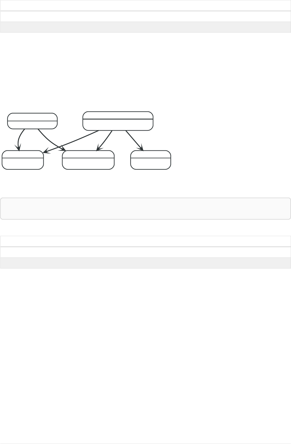
Table 68. Result
result
[0.0,1.0,8.0,27.0,64.0,125.0,216.0,343.0,512.0,729.0,1000.0]
1 row
2.11.3. Pattern comprehension
Pattern comprehension is a syntactic construct available in Cypher for creating a list based on
matchings of a pattern. A pattern comprehension will match the specified pattern just like a normal
MATCH clause, with predicates just like a normal WHERE clause, but will yield a custom projection as
specified.
The following graph is used for the example below:
Person
name = 'Charlie Sheen'
realName = 'Carlos Irwin Estévez'
Movie
year = 1979
title = 'Apocalypse Now'
ACTED_IN
Movie
year = 1984
title = 'Red Dawn'
ACTED_IN
Movie
year = 1987
title = 'Wall Street'
ACTED_IN
Person
name = 'Martin Sheen'
ACTED_INACTED_IN
Figure 4. Graph
Query
MATCH (a:Person { name: 'Charlie Sheen' })
RETURN [(a)-->(b) WHERE b:Movie | b.year] AS years
Table 69. Result
years
[1979,1984,1987]
1 row
The whole predicate, including the WHERE keyword, is optional and may be omitted.
2.12. Maps
Cypher has solid support for maps.
•Literal maps
•Map projection
•Examples of map projection
The following graph is used for the examples below:
63
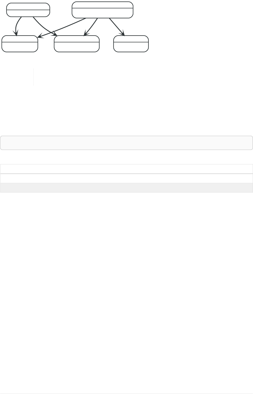
Person
name = 'Charlie Sheen'
realName = 'Carlos Irwin Estévez'
Movie
year = 1979
title = 'Apocalypse Now'
ACTED_IN
Movie
year = 1984
title = 'Red Dawn'
ACTED_IN
Movie
year = 1987
title = 'Wall Street'
ACTED_IN
Person
name = 'Martin Sheen'
ACTED_INACTED_IN
Figure 5. Graph
Information regarding property access operators such as . and [] can be found
here. The behavior of the [] operator with respect to null is detailed here.
2.12.1. Literal maps
From Cypher, you can also construct maps. Through REST you will get JSON objects; in Java they will be
java.util.Map<String,Object>.
Query
RETURN { key: 'Value', listKey: [{ inner: 'Map1' }, { inner: 'Map2' }]}
Table 70. Result
{ key: 'Value', listKey: [{ inner: 'Map1' }, { inner: 'Map2' }]}
{listKey -> [{inner -> "Map1"},{inner -> "Map2"}], key -> "Value"}
1 row
2.12.2. Map projection
Cypher supports a concept called "map projections". It allows for easily constructing map projections
from nodes, relationships and other map values.
A map projection begins with the variable bound to the graph entity to be projected from, and
contains a body of comma-separated map elements, enclosed by { and }.
map_variable {map_element, [, …n]}
A map element projects one or more key-value pairs to the map projection. There exist four different
types of map projection elements:
•Property selector - Projects the property name as the key, and the value from the map_variable as
the value for the projection.
•Literal entry - This is a key-value pair, with the value being arbitrary expression key: <expression>.
•Variable selector - Projects a variable, with the variable name as the key, and the value the variable
is pointing to as the value of the projection. Its syntax is just the variable.
•All-properties selector - projects all key-value pairs from the map_variable value.
Note that if the map_variable points to a null value, the whole map projection will evaluate to null.
Examples of map projections
Find 'Charlie Sheen' and return data about him and the movies he has acted in. This example shows
an example of map projection with a literal entry, which in turn also uses map projection inside the
64

aggregating collect().
Query
MATCH (actor:Person { name: 'Charlie Sheen' })-[:ACTED_IN]->(movie:Movie)
RETURN actor { .name, .realName, movies: collect(movie { .title, .year })}
Table 71. Result
actor
{movies -> [{year -> 1979, title -> "Apocalypse Now"},{year -> 1984, title -> "Red Dawn"},{year -> 1987, title
-> "Wall Street"}], realName -> "Carlos Irwin Estévez", name -> "Charlie Sheen"}
1 row
Find all persons that have acted in movies, and show number for each. This example introduces an
variable with the count, and uses a variable selector to project the value.
Query
MATCH (actor:Person)-[:ACTED_IN]->(movie:Movie)
WITH actor, count(movie) AS nrOfMovies
RETURN actor { .name, nrOfMovies }
Table 72. Result
actor
{nrOfMovies -> 3, name -> "Charlie Sheen"}
{nrOfMovies -> 2, name -> "Martin Sheen"}
2 rows
Again, focusing on 'Charlie Sheen', this time returning all properties from the node. Here we use an
all-properties selector to project all the node properties, and additionally, explicitly project the
property age. Since this property does not exist on the node, a null value is projected instead.
Query
MATCH (actor:Person { name: 'Charlie Sheen' })
RETURN actor { .*, .age }
Table 73. Result
actor
{realName -> "Carlos Irwin Estévez", name -> "Charlie Sheen", age -> <null>}
1 row
2.13. Spatial values
Cypher has built-in support for handling spatial values (points), and the underlying database
supports storing these point values as properties on nodes and relationships.
•Introduction
•Coordinate Reference Systems
•Geographic coordinate reference systems
65

•Cartesian coordinate reference systems
•Spatial instants
•Creating points
•Accessing components of points
•Spatial index
•Comparability and Orderability
Refer to Spatial functions for information regarding spatial functions allowing for the
creation and manipulation of spatial values.
Refer to Ordering and comparison of values for information regarding the
comparison and ordering of spatial values.
2.13.1. Introduction
Neo4j supports only one type of spatial geometry, the Point with the following characteristics:
•Each point can have either 2 or 3 dimensions. This means it contains either 2 or 3 64-bit floating
point values, which together are called the Coordinate.
•Each point will also be associated with a specific Coordinate Reference System (CRS) that
determines the meaning of the values in the Coordinate.
•Instances of Point and lists of Point can be assigned to node and relationship properties.
•Nodes with Point or List(Point) properties can be indexed using a spatial index. This is true for all
CRS (and for both 2D and 3D). There is no special syntax for creating spatial indexes, as it is
supported using the existing schema indexes.
•The distance function will work on points in all CRS and in both 2D and 3D but only if the two
points have the same CRS (and therefore also same dimension).
2.13.2. Coordinate Reference Systems
Four Coordinate Reference Systems (CRS) are supported, each of which falls within one of two types:
geographic coordinates modeling points on the earth, or cartesian coordinates modeling points in
euclidean space:
•Geographic coordinate reference systems
•WGS-84: longitude, latitude (x, y)
•WGS-84-3D: longitude, latitude, height (x, y, z)
•Cartesian coordinate reference systems
•Cartesian: x, y
•Cartesian 3D: x, y, z
Data within different coordinate systems are entirely incomparable, and cannot be implicitly
converted from one to the other. This is true even if they are both cartesian or both geographic. For
example, if you search for 3D points using a 2D range, you will get no results. However, they can be
ordered, as discussed in more detail in the section on Cypher ordering.
66

Geographic coordinate reference systems
Two Geographic Coordinate Reference Systems (CRS) are supported, modeling points on the earth:
•WGS 84 2D (http://spatialreference.org/ref/epsg/4326/)
•A 2D geographic point in the WGS 84 CRS is specified in one of two ways:
•longitude and latitude (if these are specified, and the crs is not, then the crs is assumed
to be WGS-84)
•x and y (in this case the crs must be specified, or will be assumed to be Cartesian)
•Specifying this CRS can be done using either the name 'wgs-84' or the SRID 4326 as described
in Point(WGS-84)
•WGS 84 3D (http://spatialreference.org/ref/epsg/4979/)
•A 3D geographic point in the WGS 84 CRS is specified one of in two ways:
•longitude, latitude and either height or z (if these are specified, and the crs is not, then
the crs is assumed to be WGS-84-3D)
•x, y and z (in this case the crs must be specified, or will be assumed to be Cartesian-3D)
•Specifying this CRS can be done using either the name 'wgs-84-3d' or the SRID 4979 as
described in Point(WGS-84-3D)
The units of the latitude and longitude fields are in decimal degrees, and need to be specified as
floating point numbers using Cypher literals. It is not possible to use any other format, like 'degrees,
minutes, seconds'. The units of the height field are in meters. When geographic points are passed to
the distance function, the result will always be in meters. If the coordinates are in any other format or
unit than supported, it is necessary to explicitly convert them. For example, if the incoming $height is
a string field in kilometers, you would need to type height: toFloat($height) * 1000. Likewise if the
results of the distance function are expected to be returned in kilometers, an explicit conversion is
required. For example: RETURN distance(a,b) / 1000 AS km. An example demonstrating conversion on
incoming and outgoing values is:
Query
WITH point({ latitude:toFloat('13.43'), longitude:toFloat('56.21')}) AS p1, point({
latitude:toFloat('13.10'), longitude:toFloat('56.41')}) AS p2
RETURN toInteger(distance(p1,p2)/1000) AS km
Table 74. Result
km
42
1 row
Cartesian coordinate reference systems
Two Cartesian Coordinate Reference Systems (CRS) are supported, modeling points in euclidean
space:
•Cartesian 2D (http://spatialreference.org/ref/sr-org/7203/)
•A 2D point in the Cartesian CRS is specified with a map containing x and y coordinate values
•Specifying this CRS can be done using either the name 'cartesian' or the SRID 7203 as
described in Point(Cartesian)
67

•Cartesian 3D (http://spatialreference.org/ref/sr-org/9157/)
•A 3D point in the Cartesian CRS is specified with a map containing x, y and z coordinate values
•Specifying this CRS can be done using either the name 'cartesian-3d' or the SRID 9157 as
described in Point(Cartesian-3D)
The units of the x, y and z fields are unspecified and can mean anything the user intends them to
mean. This also means that when two cartesian points are passed to the distance function, the
resulting value will be in the same units as the original coordinates. This is true for both 2D and 3D
points, as the pythagoras equation used is generalized to any number of dimensions. However, just as
you cannot compare geographic points to cartesian points, you cannot calculate the distance between
a 2D point and a 3D point. If you need to do that, explicitly transform the one type into the other. For
example:
Query
WITH point({ x:3, y:0 }) AS p2d, point({ x:0, y:4, z:1 }) AS p3d
RETURN distance(p2d,p3d) AS bad, distance(p2d,point({ x:p3d.x, y:p3d.y })) AS good
Table 75. Result
bad good
<null> 5.0
1 row
2.13.3. Spatial instants
Creating points
All point types are created from two components:
•The Coordinate containing either 2 or 3 floating point values (64-bit)
•The Coordinate Reference System (or CRS) defining the meaning (and possibly units) of the values
in the Coordinate
For most use cases it is not necessary to specify the CRS explicitly as it will be deduced from the keys
used to specify the coordinate. Two rules are applied to deduce the CRS from the coordinate:
•Choice of keys:
•If the coordinate is specified using the keys latitude and longitude the CRS will be assumed to
be Geographic and therefor either WGS-84 or WGS-84-3D.
•If instead x and y are used, then the default CRS would be Cartesian or Cartesian-3D
•Number of dimensions:
•If there are 2 dimensions in the coordinate, x & y or longitude & latitude the CRS will be a 2D
CRS
•If there is a third dimensions in the coordinate, z or height the CRS will be a 3D CRS
All fields are provided to the point function in the form of a map of explicitly named arguments. We
specifically do not support an ordered list of coordinate fields because of the contradictory
conventions between geographic and cartesian coordinates, where geographic coordinates normally
list y before x (latitude before longitude). See for example the following query which returns points
created in each of the four supported CRS. Take particular note of the order and keys of the
coordinates in the original point function calls, and how those values are displayed in the results:
68

Query
RETURN point({ x:3, y:0 }) AS cartesian_2d, point({ x:0, y:4, z:1 }) AS cartesian_3d, point({ latitude:
12, longitude: 56 }) AS geo_2d, point({ latitude: 12, longitude: 56, height: 1000 }) AS geo_3d
Table 76. Result
cartesian_2d cartesian_3d geo_2d geo_3d
point({x: 3.0, y: 0.0,
crs: 'cartesian'})
point({x: 0.0, y: 4.0, z:
1.0, crs: 'cartesian-3d'})
point({x: 56.0, y: 12.0,
crs: 'wgs-84'})
point({x: 56.0, y: 12.0,
z: 1000.0, crs: 'wgs-84-
3d'})
1 row
Accessing components of points
Just as we construct points using a map syntax, we can also access components as properties of the
instance.
Table 77. Components of point instances and where they are supported
Component Description Type Range/Form
at
WGS-84 WGS-84-3D Cartesian Cartesian-3D
instant.x The first
element of
the
Coordinate
Float Number
literal, range
depends on
CRS
XXXX
instant.y The second
element of
the
Coordinate
Float Number
literal, range
depends on
CRS
XXXX
instant.z The third
element of
the
Coordinate
Float Number
literal, range
depends on
CRS
X X
instant.lati
tude
The second
element of
the
Coordinate
for
geographic
CRS, degrees
North of the
equator
Float Number
literal, -90.0
to 90.0
X X
instant.long
itude
The first
element of
the
Coordinate
for
geographic
CRS, degrees
East of the
prime
meridian
Float Number
literal, -180.0
to 180.0
X X
instant.heig
ht
The third
element of
the
Coordinate
for
geographic
CRS, meters
above the
ellipsoid
defined by
the datum
(WGS-84)
Float Number
literal, range
limited only
by the
underlying
64-bit
floating point
type
X
69

Component Description Type Range/Form
at
WGS-84 WGS-84-3D Cartesian Cartesian-3D
instant.crs The name of
the CRS
String One of wgs-
84, wgs-84-3d,
cartesian,
cartesian-3d
XXXX
instant.srid The internal
Neo4j ID for
the CRS
Integer One of 4326,
4979, 7203,
9157
XXXX
The following query shows how to extract the components of a Cartesian 2D point value:
Query
WITH point({ x:3, y:4 }) AS p
RETURN p.x, p.y, p.crs, p.srid
Table 78. Result
p.x p.y p.crs p.srid
3.0 4.0 "cartesian" 7203
1 row
The following query shows how to extract the components of a WGS-84 3D point value:
Query
WITH point({ latitude:3, longitude:4, height: 4321 }) AS p
RETURN p.latitude, p.longitude, p.height, p.x, p.y, p.z, p.crs, p.srid
Table 79. Result
p.latitude p.longitude p.height p.x p.y p.z p.crs p.srid
3.0 4.0 4321.0 4.0 3.0 4321.0 "wgs-84-3d" 4979
1 row
2.13.4. Spatial index
If there is a schema index on a particular :Label(property) combination, and a spatial point is
assigned to that property on a node with that label, the node will be indexed in a spatial index. For
spatial indexing, Neo4j uses space filling curves in 2D or 3D over an underlying generalized B+Tree.
Points will be stored in up to four different trees, one for each of the four coordinate reference
systems. This allows for both equality and range queries using exactly the same syntax and behaviour
as for other property types. If two range predicates are used, which define minimum and maximum
points, this will effectively result in a bounding box query. In addition, queries using the distance
function can, under the right conditions, also use the index, as described in the section 'Spatial
distance searches'.
2.13.5. Comparability and Orderability
Points with different CRS are not comparable. This means that any function operating on two points of
different types will return null. This is true of the distance function as well as inequality comparisons.
If these are used in a predicate, they will cause the associated MATCH to return no results.
70

Query
WITH point({ x:3, y:0 }) AS p2d, point({ x:0, y:4, z:1 }) AS p3d
RETURN distance(p2d,p3d), p2d < p3d, p2d = p3d, p2d <> p3d, distance(p2d,point({ x:p3d.x, y:p3d.y }))
Table 80. Result
distance(p2d,p3d) p2d < p3d p2d = p3d p2d <> p3d distance(p2d,point({
x:p3d.x, y:p3d.y }))
<null> <null> false true 5.0
1 row
However, all types are orderable. The Point types will be ordered after Numbers and before Temporal
types. Points with different CRS with be ordered by their SRID numbers. For the current set of four
CRS, this means the order is WGS84, WGS84-3D, Cartesian, Cartesian-3D.
Query
UNWIND [point({ x:3, y:0 }), point({ x:0, y:4, z:1 }), point({ srid:4326, x:12, y:56 }), point({
srid:4979, x:12, y:56, z:1000 })] AS point
RETURN point
ORDER BY point
Table 81. Result
point
point({x: 12.0, y: 56.0, crs: 'wgs-84'})
point({x: 12.0, y: 56.0, z: 1000.0, crs: 'wgs-84-3d'})
point({x: 3.0, y: 0.0, crs: 'cartesian'})
point({x: 0.0, y: 4.0, z: 1.0, crs: 'cartesian-3d'})
4 rows
2.14. Working with null
•Introduction to null in Cypher
•Logical operations with null
•The IN operator and null
•The [] operator and null
•Expressions that return null
2.14.1. Introduction to null in Cypher
In Cypher, null is used to represent missing or undefined values. Conceptually, null means 'a missing
unknown value' and it is treated somewhat differently from other values. For example getting a
property from a node that does not have said property produces null. Most expressions that take
null as input will produce null. This includes boolean expressions that are used as predicates in the
WHERE clause. In this case, anything that is not true is interpreted as being false.
null is not equal to null. Not knowing two values does not imply that they are the same value. So the
expression null = null yields null and not true.
71

2.14.2. Logical operations with null
The logical operators (AND, OR, XOR, NOT) treat null as the 'unknown' value of three-valued logic.
Here is the truth table for AND, OR, XOR and NOT.
a b a AND b a OR b a XOR b NOT a
false false false false false true
false null false null null true
false true false true true true
true false false true true false
true null null true null false
true true true true false false
null false false null null null
null null null null null null
null true null true null null
2.14.3. The IN operator and null
The IN operator follows similar logic. If Cypher knows that something exists in a list, the result will be
true. Any list that contains a null and doesn’t have a matching element will return null. Otherwise,
the result will be false. Here is a table with examples:
Expression Result
2 IN [1, 2, 3] true
2 IN [1, null, 3] null
2 IN [1, 2, null]true
2 IN [1] false
2 IN [] false
null IN [1, 2, 3] null
null IN [1, null, 3] null
null IN [] false
Using all, any, none, and single follows a similar rule. If the result can be calculated definitely, true or
false is returned. Otherwise null is produced.
2.14.4. The [] operator and null
Accessing a list or a map with null will result in null:
Expression Result
[1, 2, 3][null]null
[1, 2, 3, 4][null..2] null
[1, 2, 3][1..null]null
{age: 25}[null]null
Using parameters to pass in the bounds, such as a[$lower..$upper], may result in a null for the lower
72

or upper bound (or both). The following workaround will prevent this from happening by setting the
absolute minimum and maximum bound values:
a[coalesce($lower,0)..coalesce($upper,size(a))]
2.14.5. Expressions that return null
•Getting a missing element from a list: [][0], head([])
•Trying to access a property that does not exist on a node or relationship: n.missingProperty
•Comparisons when either side is null: 1 < null
•Arithmetic expressions containing null: 1 + null
•Function calls where any arguments are null: sin(null)
73

Chapter 3. Clauses
This section contains information on all the clauses in the Cypher query language.
•Reading clauses
•Projecting clauses
•Reading sub-clauses
•Reading hints
•Writing clauses
•Reading/Writing clauses
•Set operations
•Importing data
•Schema clauses
Reading clauses
These comprise clauses that read data from the database.
The flow of data within a Cypher query is an unordered sequence of maps with key-value pairs — a set
of possible bindings between the variables in the query and values derived from the database. This
set is refined and augmented by subsequent parts of the query.
Clause Description
MATCH Specify the patterns to search for in the database.
OPTIONAL MATCH Specify the patterns to search for in the database while
using nulls for missing parts of the pattern.
START Find starting points through legacy indexes.
Projecting clauses
These comprise clauses that define which expressions to return in the result set. The returned
expressions may all be aliased using AS.
Clause Description
RETURN … [AS] Defines what to include in the query result set.
WITH … [AS] Allows query parts to be chained together, piping the
results from one to be used as starting points or criteria in
the next.
UNWIND … [AS] Expands a list into a sequence of rows.
Reading sub-clauses
These comprise sub-clauses that must operate as part of reading clauses.
Sub-clause Description
WHERE Adds constraints to the patterns in a MATCH or OPTIONAL
MATCH clause or filters the results of a WITH clause.
ORDER BY [ASC[ENDING] | DESC[ENDING]] A sub-clause following RETURN or WITH, specifying that the
output should be sorted in either ascending (the default)
or descending order.
74
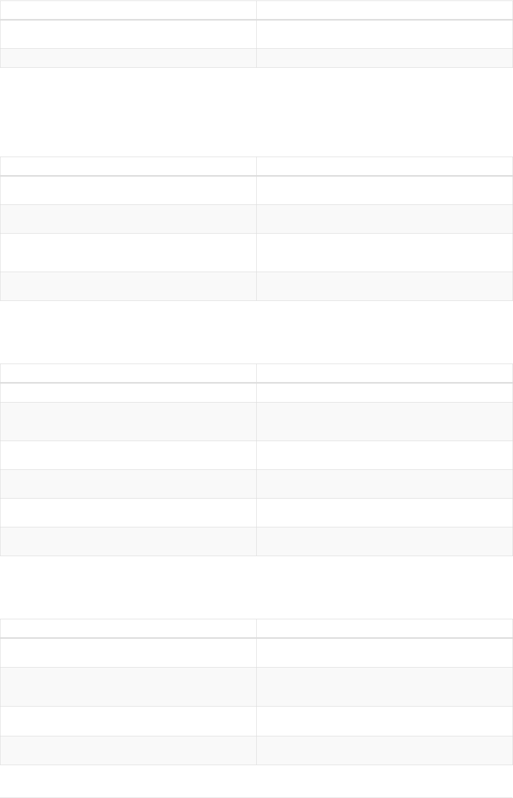
Sub-clause Description
SKIP Defines from which row to start including the rows in the
output.
LIMIT Constrains the number of rows in the output.
Reading hints
These comprise clauses used to specify planner hints when tuning a query. More details regarding the
usage of these — and query tuning in general — can be found in Planner hints and the USING
keyword.
Hint Description
USING INDEX Index hints are used to specify which index, if any, the
planner should use as a starting point.
USING INDEX SEEK Index seek hint instructs the planner to use an index seek
for this clause.
USING SCAN Scan hints are used to force the planner to do a label scan
(followed by a filtering operation) instead of using an
index.
USING JOIN Join hints are used to enforce a join operation at specified
points.
Writing clauses
These comprise clauses that write the data to the database.
Clause Description
CREATE Create nodes and relationships.
DELETE Delete nodes, relationships or paths. Any node to be
deleted must also have all associated relationships
explicitly deleted.
DETACH DELETE Delete a node or set of nodes. All associated relationships
will automatically be deleted.
SET Update labels on nodes and properties on nodes and
relationships.
REMOVE Remove properties and labels from nodes and
relationships.
FOREACH Update data within a list, whether components of a path,
or the result of aggregation.
Reading/Writing clauses
These comprise clauses that both read data from and write data to the database.
Clause Description
MERGE Ensures that a pattern exists in the graph. Either the
pattern already exists, or it needs to be created.
--- ON CREATE Used in conjunction with MERGE, this write sub-clause
specifies the actions to take if the pattern needs to be
created.
--- ON MATCH Used in conjunction with MERGE, this write sub-clause
specifies the actions to take if the pattern already exists.
CALL […YIELD] Invoke a procedure deployed in the database and return
any results.
75

Clause Description
CREATE UNIQUE A mixture of MATCH and CREATE, matching what it can, and
creating what is missing.
Set operations
Clause Description
UNION Combines the result of multiple queries into a single result
set. Duplicates are removed.
UNION ALL Combines the result of multiple queries into a single result
set. Duplicates are retained.
Importing data
Clause Description
LOAD CSV Use when importing data from CSV files.
--- USING PERIODIC COMMIT This query hint may be used to prevent an out-of-memory
error from occurring when importing large amounts of
data using LOAD CSV.
Schema clauses
These comprise clauses used to manage the schema; further details can found in Schema.
Clause Description
CREATE | DROP CONSTRAINT Create or drop an index on all nodes with a particular label
and property.
CREATE | DROP INDEX Create or drop a constraint pertaining to either a node
label or relationship type, and a property.
3.1. MATCH
The MATCH clause is used to search for the pattern described in it.
•Introduction
•Basic node finding
•Get all nodes
•Get all nodes with a label
•Related nodes
•Match with labels
•Relationship basics
•Outgoing relationships
•Directed relationships and variable
•Match on relationship type
•Match on multiple relationship types
•Match on relationship type and use a variable
•Relationships in depth
76

•Relationship types with uncommon characters
•Multiple relationships
•Variable length relationships
•Relationship variable in variable length relationships
•Match with properties on a variable length path
•Zero length paths
•Named paths
•Matching on a bound relationship
•Shortest path
•Single shortest path
•Single shortest path with predicates
•All shortest paths
•Get node or relationship by id
•Node by id
•Relationship by id
•Multiple nodes by id
3.1.1. Introduction
The MATCH clause allows you to specify the patterns Neo4j will search for in the database. This is the
primary way of getting data into the current set of bindings. It is worth reading up more on the
specification of the patterns themselves in Patterns.
MATCH is often coupled to a WHERE part which adds restrictions, or predicates, to the MATCH patterns,
making them more specific. The predicates are part of the pattern description, and should not be
considered a filter applied only after the matching is done. This means that WHERE should always be put
together with the MATCH clause it belongs to.
MATCH can occur at the beginning of the query or later, possibly after a WITH. If it is the first clause,
nothing will have been bound yet, and Neo4j will design a search to find the results matching the
clause and any associated predicates specified in any WHERE part. This could involve a scan of the
database, a search for nodes having a certain label, or a search of an index to find starting points for
the pattern matching. Nodes and relationships found by this search are available as bound pattern
elements, and can be used for pattern matching of sub-graphs. They can also be used in any further
MATCH clauses, where Neo4j will use the known elements, and from there find further unknown
elements.
Cypher is declarative, and so usually the query itself does not specify the algorithm to use to perform
the search. Neo4j will automatically work out the best approach to finding start nodes and matching
patterns. Predicates in WHERE parts can be evaluated before pattern matching, during pattern
matching, or after finding matches. However, there are cases where you can influence the decisions
taken by the query compiler. Read more about indexes in Indexes, and more about specifying hints to
force Neo4j to solve a query in a specific way in Planner hints and the USING keyword.
To understand more about the patterns used in the MATCH clause, read Patterns
The following graph is used for the examples below:
77
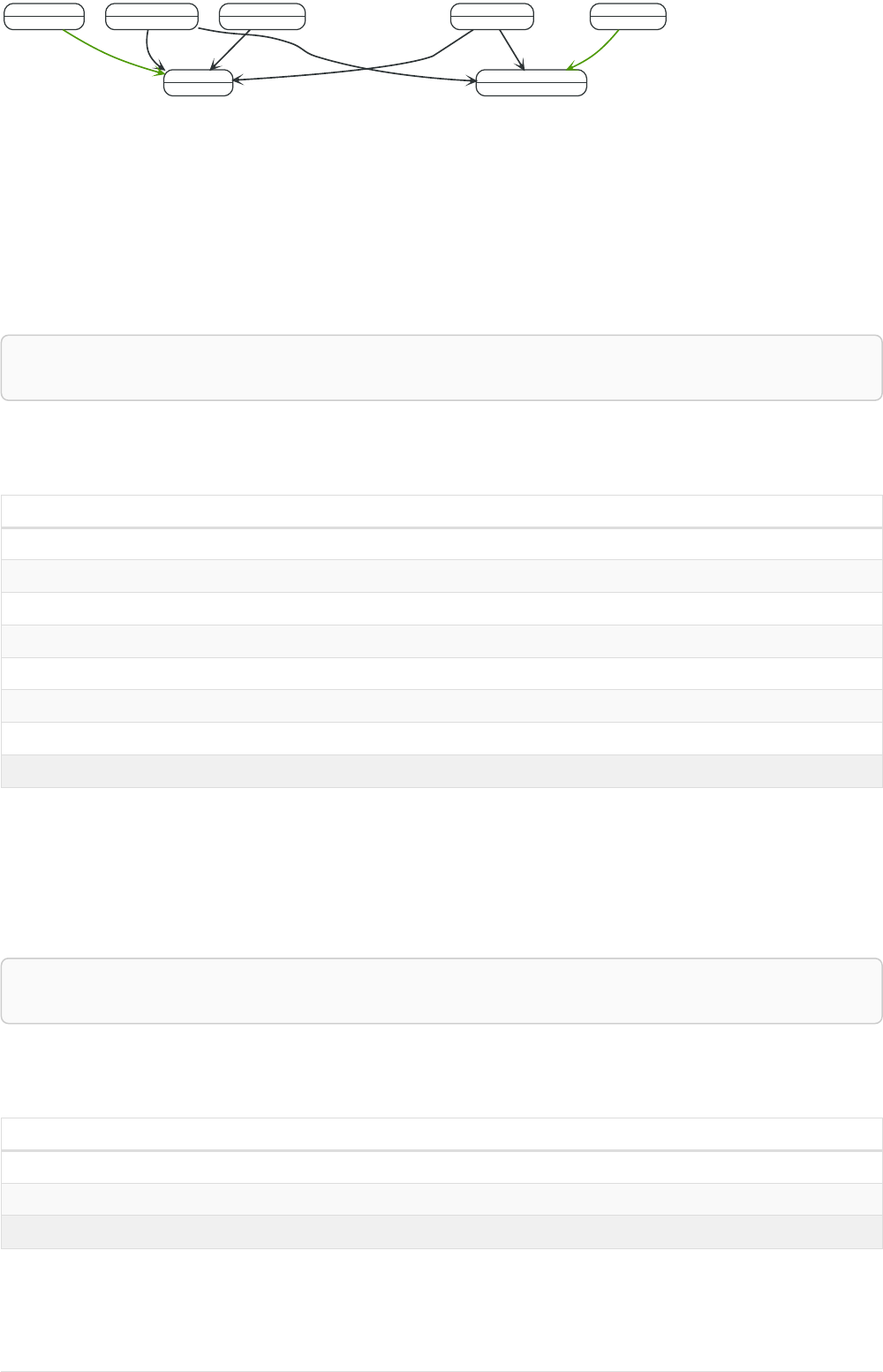
Person
name = 'Charlie Sheen'
Movie
title = 'Wall Street'
ACTED_IN
role = 'Bud Fox'
Person
name = 'Martin Sheen'
ACTED_IN
role = 'Carl Fox'
Movie
title = 'The American President'
ACTED_IN
role = 'A.J. MacInerney'
Person
name = 'Michael Douglas'
ACTED_IN
role = 'Gordon Gekko' ACTED_IN
role = 'President Andrew Shepherd'
Person
name = 'Oliver Stone'
DIRECTED
Person
name = 'Rob Reiner'
DIRECTED
Figure 6. Graph
3.1.2. Basic node finding
Get all nodes
By just specifying a pattern with a single node and no labels, all nodes in the graph will be returned.
Query
MATCH (n)
RETURN n
Returns all the nodes in the database.
Table 82. Result
n
Node[0]{name:"Charlie Sheen"}
Node[1]{name:"Martin Sheen"}
Node[2]{name:"Michael Douglas"}
Node[3]{name:"Oliver Stone"}
Node[4]{name:"Rob Reiner"}
Node[5]{title:"Wall Street"}
Node[6]{title:"The American President"}
7 rows
Get all nodes with a label
Getting all nodes with a label on them is done with a single node pattern where the node has a label
on it.
Query
MATCH (movie:Movie)
RETURN movie.title
Returns all the movies in the database.
Table 83. Result
movie.title
"Wall Street"
"The American President"
2 rows
78

Related nodes
The symbol -- means related to, without regard to type or direction of the relationship.
Query
MATCH (director { name: 'Oliver Stone' })--(movie)
RETURN movie.title
Returns all the movies directed by 'Oliver Stone'.
Table 84. Result
movie.title
"Wall Street"
1 row
Match with labels
To constrain your pattern with labels on nodes, you add it to your pattern nodes, using the label
syntax.
Query
MATCH (:Person { name: 'Oliver Stone' })--(movie:Movie)
RETURN movie.title
Returns any nodes connected with the Person 'Oliver' that are labeled Movie.
Table 85. Result
movie.title
"Wall Street"
1 row
3.1.3. Relationship basics
Outgoing relationships
When the direction of a relationship is of interest, it is shown by using -→ or ←-, like this:
Query
MATCH (:Person { name: 'Oliver Stone' })-->(movie)
RETURN movie.title
Returns any nodes connected with the Person 'Oliver' by an outgoing relationship.
Table 86. Result
movie.title
"Wall Street"
1 row
79

Directed relationships and variable
If a variable is required, either for filtering on properties of the relationship, or to return the
relationship, this is how you introduce the variable.
Query
MATCH (:Person { name: 'Oliver Stone' })-[r]->(movie)
RETURN type(r)
Returns the type of each outgoing relationship from 'Oliver'.
Table 87. Result
type(r)
"DIRECTED"
1 row
Match on relationship type
When you know the relationship type you want to match on, you can specify it by using a colon
together with the relationship type.
Query
MATCH (wallstreet:Movie { title: 'Wall Street' })<-[:ACTED_IN]-(actor)
RETURN actor.name
Returns all actors that ACTED_IN 'Wall Street'.
Table 88. Result
actor.name
"Michael Douglas"
"Martin Sheen"
"Charlie Sheen"
3 rows
Match on multiple relationship types
To match on one of multiple types, you can specify this by chaining them together with the pipe
symbol |.
Query
MATCH (wallstreet { title: 'Wall Street' })<-[:ACTED_IN|:DIRECTED]-(person)
RETURN person.name
Returns nodes with an ACTED_IN or DIRECTED relationship to 'Wall Street'.
Table 89. Result
person.name
"Oliver Stone"
"Michael Douglas"
80
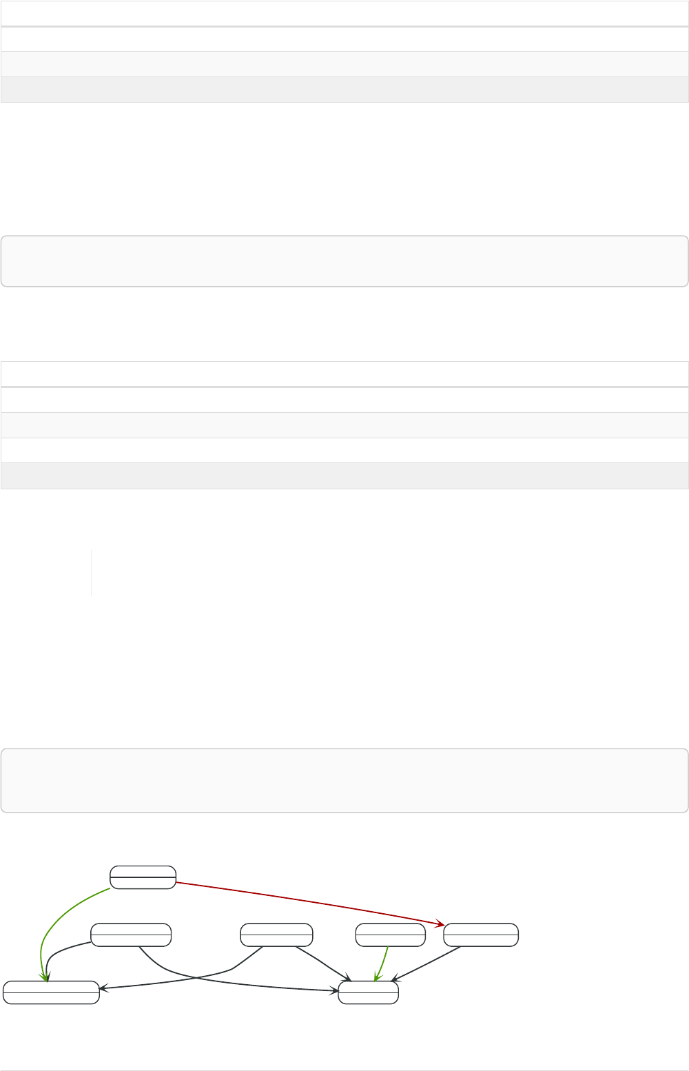
person.name
"Martin Sheen"
"Charlie Sheen"
4 rows
Match on relationship type and use a variable
If you both want to introduce an variable to hold the relationship, and specify the relationship type
you want, just add them both, like this:
Query
MATCH (wallstreet { title: 'Wall Street' })<-[r:ACTED_IN]-(actor)
RETURN r.role
Returns ACTED_IN roles for 'Wall Street'.
Table 90. Result
r.role
"Gordon Gekko"
"Carl Fox"
"Bud Fox"
3 rows
3.1.4. Relationships in depth
Inside a single pattern, relationships will only be matched once. You can read more
about this in Uniqueness.
Relationship types with uncommon characters
Sometimes your database will have types with non-letter characters, or with spaces in them. Use `
(backtick) to quote these. To demonstrate this we can add an additional relationship between 'Charlie
Sheen' and 'Rob Reiner':
Query
MATCH (charlie:Person { name: 'Charlie Sheen' }),(rob:Person { name: 'Rob Reiner' })
CREATE (rob)-[:`TYPE
WITH SPACE`]->(charlie)
Which leads to the following graph:
Person
name = 'Charlie Sheen'
Movie
title = 'Wall Street'
ACTED_IN
role = 'Bud Fox'
Person
name = 'Martin Sheen'
ACTED_IN
role = 'Carl Fox'
Movie
title = 'The American President'
ACTED_IN
role = 'A.J. MacInerney'
Person
name = 'Michael Douglas'
ACTED_IN
role = 'Gordon Gekko'
ACTED_IN
role = 'President Andrew Shepherd'
Person
name = 'Oliver Stone'
DIRECTED
Person
name = 'Rob Reiner'
TYPE
WITH SPACE
DIRECTED
Figure 7. Graph
81

Query
MATCH (n { name: 'Rob Reiner' })-[r:`TYPE
WITH SPACE`]->()
RETURN type(r)
Returns a relationship type with a space in it
Table 91. Result
type(r)
"TYPE WITH SPACE"
1 row
Multiple relationships
Relationships can be expressed by using multiple statements in the form of ()--(), or they can be
strung together, like this:
Query
MATCH (charlie { name: 'Charlie Sheen' })-[:ACTED_IN]->(movie)<-[:DIRECTED]-(director)
RETURN movie.title, director.name
Returns the movie 'Charlie Sheen' acted in and its director.
Table 92. Result
movie.title director.name
"Wall Street" "Oliver Stone"
1 row
Variable length relationships
Nodes that are a variable number of relationship→node hops away can be found using the following
syntax: -[:TYPE*minHops..maxHops]→. minHops and maxHops are optional and default to 1 and infinity
respectively. When no bounds are given the dots may be omitted. The dots may also be omitted
when setting only one bound and this implies a fixed length pattern.
Query
MATCH (martin { name: 'Charlie Sheen' })-[:ACTED_IN*1..3]-(movie:Movie)
RETURN movie.title
Returns all movies related to 'Charlie Sheen' by 1 to 3 hops.
Table 93. Result
movie.title
"Wall Street"
"The American President"
"The American President"
3 rows
82
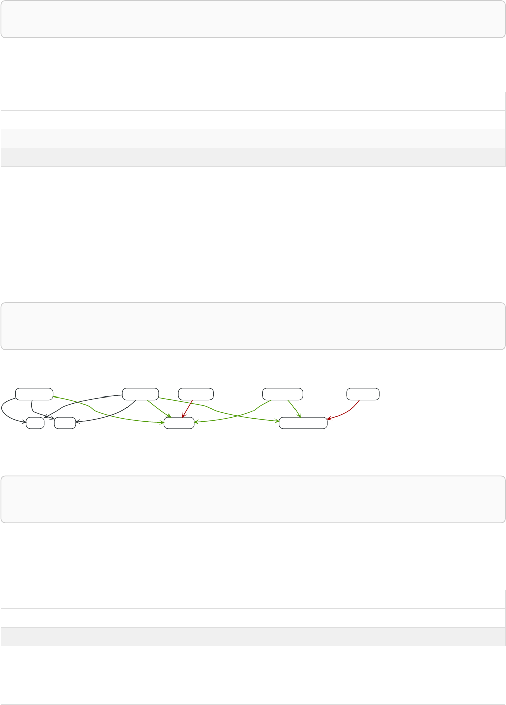
Relationship variable in variable length relationships
When the connection between two nodes is of variable length, the list of relationships comprising the
connection can be returned using the following syntax:
Query
MATCH p =(actor { name: 'Charlie Sheen' })-[:ACTED_IN*2]-(co_actor)
RETURN relationships(p)
Returns a list of relationships.
Table 94. Result
relationships(p)
[:ACTED_IN[0]{role:"Bud Fox"},:ACTED_IN[1]{role:"Carl Fox"}]
[:ACTED_IN[0]{role:"Bud Fox"},:ACTED_IN[2]{role:"Gordon Gekko"}]
2 rows
Match with properties on a variable length path
A variable length relationship with properties defined on in it means that all relationships in the path
must have the property set to the given value. In this query, there are two paths between 'Charlie
Sheen' and his father 'Martin Sheen'. One of them includes a 'blocked' relationship and the other
doesn’t. In this case we first alter the original graph by using the following query to add BLOCKED and
UNBLOCKED relationships:
Query
MATCH (charlie:Person { name: 'Charlie Sheen' }),(martin:Person { name: 'Martin Sheen' })
CREATE (charlie)-[:X { blocked: FALSE }]->(:UNBLOCKED)<-[:X { blocked: FALSE }]-(martin)
CREATE (charlie)-[:X { blocked: TRUE }]->(:BLOCKED)<-[:X { blocked: FALSE }]-(martin)
This means that we are starting out with the following graph:
Person
name = 'Charlie Sheen'
BLOCKED
X
blocked = true
UNBLOCKED
X
blocked = false
Movie
title = 'Wall Street'
ACTED_IN
role = 'Bud Fox'
Person
name = 'Martin Sheen'
X
blocked = false X
blocked = false ACTED_IN
role = 'Carl Fox'
Movie
title = 'The American President'
ACTED_IN
role = 'A.J. MacInerney'
Person
name = 'Michael Douglas'
ACTED_IN
role = 'Gordon Gekko' ACTED_IN
role = 'President Andrew Shepherd'
Person
name = 'Oliver Stone'
DIRECTED
Person
name = 'Rob Reiner'
DIRECTED
Figure 8. Graph
Query
MATCH p =(charlie:Person)-[* { blocked:false }]-(martin:Person)
WHERE charlie.name = 'Charlie Sheen' AND martin.name = 'Martin Sheen'
RETURN p
Returns the paths between 'Charlie Sheen' and 'Martin Sheen' where all relationships have the
blocked property set to false.
Table 95. Result
p
(0)-[X,20]->(20)<-[X,21]-(1)
1 row
83

Zero length paths
Using variable length paths that have the lower bound zero means that two variables can point to the
same node. If the path length between two nodes is zero, they are by definition the same node. Note
that when matching zero length paths the result may contain a match even when matching on a
relationship type not in use.
Query
MATCH (wallstreet:Movie { title: 'Wall Street' })-[*0..1]-(x)
RETURN x
Returns the movie itself as well as actors and directors one relationship away
Table 96. Result
x
Node[5]{title:"Wall Street"}
Node[0]{name:"Charlie Sheen"}
Node[1]{name:"Martin Sheen"}
Node[2]{name:"Michael Douglas"}
Node[3]{name:"Oliver Stone"}
5 rows
Named paths
If you want to return or filter on a path in your pattern graph, you can a introduce a named path.
Query
MATCH p =(michael { name: 'Michael Douglas' })-->()
RETURN p
Returns the two paths starting from 'Michael Douglas'
Table 97. Result
p
(2)-[ACTED_IN,5]->(6)
(2)-[ACTED_IN,2]->(5)
2 rows
Matching on a bound relationship
When your pattern contains a bound relationship, and that relationship pattern doesn’t specify
direction, Cypher will try to match the relationship in both directions.
Query
MATCH (a)-[r]-(b)
WHERE id(r)= 0
RETURN a,b
This returns the two connected nodes, once as the start node, and once as the end node
84

Table 98. Result
a b
Node[0]{name:"Charlie Sheen"} Node[5]{title:"Wall Street"}
Node[5]{title:"Wall Street"} Node[0]{name:"Charlie Sheen"}
2 rows
3.1.5. Shortest path
Single shortest path
Finding a single shortest path between two nodes is as easy as using the shortestPath function. It’s
done like this:
Query
MATCH (martin:Person { name: 'Martin Sheen' }),(oliver:Person { name: 'Oliver Stone' }), p =
shortestPath((martin)-[*..15]-(oliver))
RETURN p
This means: find a single shortest path between two nodes, as long as the path is max 15
relationships long. Within the parentheses you define a single link of a path — the starting node, the
connecting relationship and the end node. Characteristics describing the relationship like relationship
type, max hops and direction are all used when finding the shortest path. If there is a WHERE clause
following the match of a shortestPath, relevant predicates will be included in the shortestPath. If the
predicate is a none() or all() on the relationship elements of the path, it will be used during the
search to improve performance (see Shortest path planning).
Table 99. Result
p
(1)-[ACTED_IN,1]->(5)<-[DIRECTED,3]-(3)
1 row
Single shortest path with predicates
Predicates used in the WHERE clause that apply to the shortest path pattern are evaluated before
deciding what the shortest matching path is.
Query
MATCH (charlie:Person { name: 'Charlie Sheen' }),(martin:Person { name: 'Martin Sheen' }), p =
shortestPath((charlie)-[*]-(martin))
WHERE NONE (r IN relationships(p) WHERE type(r)= 'FATHER')
RETURN p
This query will find the shortest path between 'Charlie Sheen' and 'Martin Sheen', and the WHERE
predicate will ensure that we don’t consider the father/son relationship between the two.
Table 100. Result
p
(0)-[ACTED_IN,0]->(5)<-[ACTED_IN,1]-(1)
1 row
85

All shortest paths
Finds all the shortest paths between two nodes.
Query
MATCH (martin:Person { name: 'Martin Sheen' }),(michael:Person { name: 'Michael Douglas' }), p =
allShortestPaths((martin)-[*]-(michael))
RETURN p
Finds the two shortest paths between 'Martin Sheen' and 'Michael Douglas'.
Table 101. Result
p
(1)-[ACTED_IN,1]->(5)<-[ACTED_IN,2]-(2)
(1)-[ACTED_IN,4]->(6)<-[ACTED_IN,5]-(2)
2 rows
3.1.6. Get node or relationship by id
Node by id
Searching for nodes by id can be done with the id() function in a predicate.
Neo4j reuses its internal ids when nodes and relationships are deleted. This means
that applications using, and relying on internal Neo4j ids, are brittle or at risk of
making mistakes. It is therefore recommended to rather use application-generated
ids.
Query
MATCH (n)
WHERE id(n)= 0
RETURN n
The corresponding node is returned.
Table 102. Result
n
Node[0]{name:"Charlie Sheen"}
1 row
Relationship by id
Search for relationships by id can be done with the id() function in a predicate.
This is not recommended practice. See Node by id for more information on the use of Neo4j ids.
Query
MATCH ()-[r]->()
WHERE id(r)= 0
RETURN r
86

The relationship with id 0 is returned.
Table 103. Result
r
:ACTED_IN[0]{role:"Bud Fox"}
1 row
Multiple nodes by id
Multiple nodes are selected by specifying them in an IN clause.
Query
MATCH (n)
WHERE id(n) IN [0, 3, 5]
RETURN n
This returns the nodes listed in the IN expression.
Table 104. Result
n
Node[0]{name:"Charlie Sheen"}
Node[3]{name:"Oliver Stone"}
Node[5]{title:"Wall Street"}
3 rows
3.2. OPTIONAL MATCH
The OPTIONAL MATCH clause is used to search for the pattern described in it, while using nulls
for missing parts of the pattern.
•Introduction
•Optional relationships
•Properties on optional elements
•Optional typed and named relationship
3.2.1. Introduction
OPTIONAL MATCH matches patterns against your graph database, just like MATCH does. The difference is
that if no matches are found, OPTIONAL MATCH will use a null for missing parts of the pattern. OPTIONAL
MATCH could be considered the Cypher equivalent of the outer join in SQL.
Either the whole pattern is matched, or nothing is matched. Remember that WHERE is part of the
pattern description, and the predicates will be considered while looking for matches, not after. This
matters especially in the case of multiple (OPTIONAL) MATCH clauses, where it is crucial to put WHERE
together with the MATCH it belongs to.
To understand the patterns used in the OPTIONAL MATCH clause, read Patterns.
The following graph is used for the examples below:
87
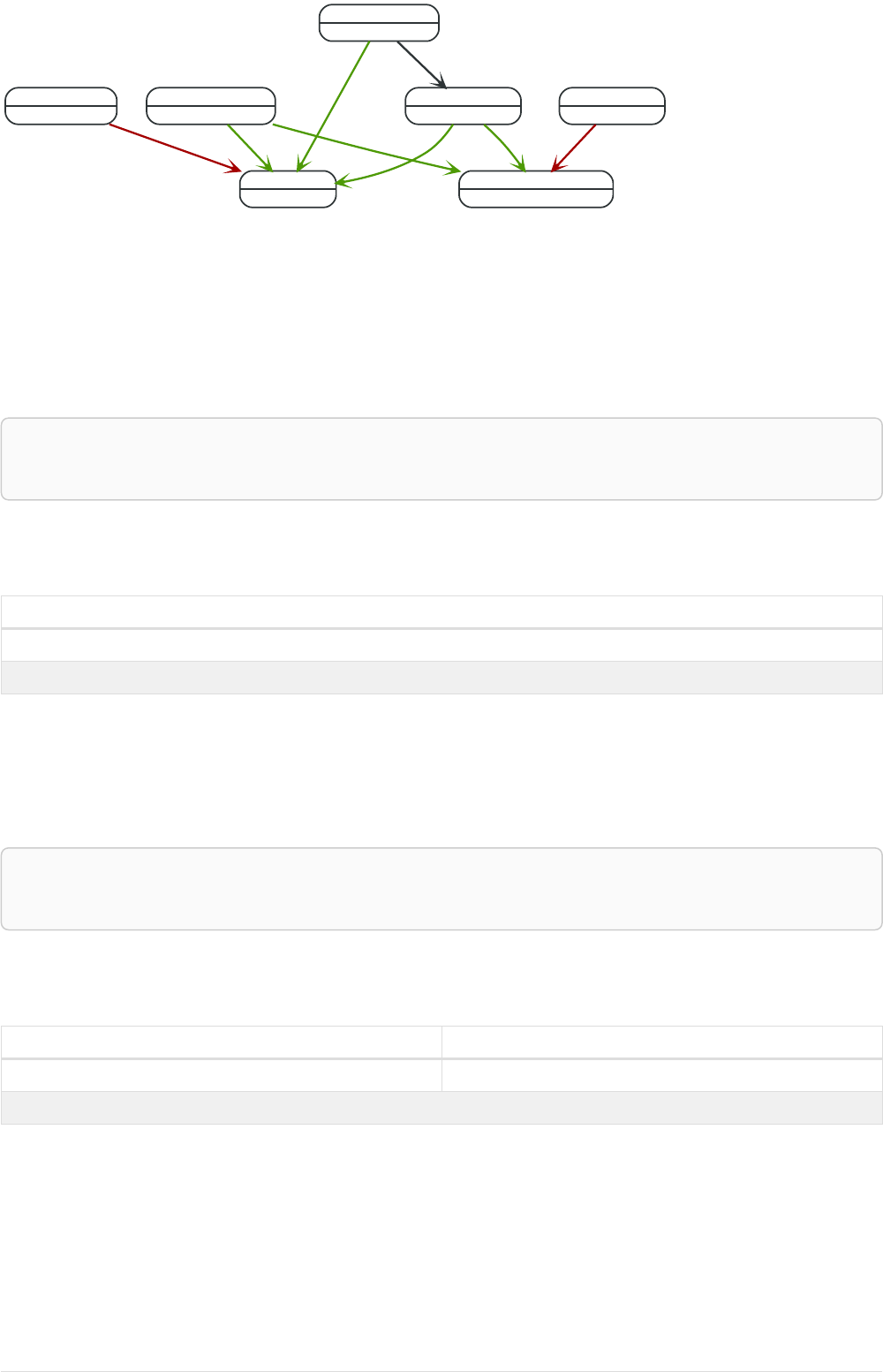
Person
name = 'Charlie Sheen'
Person
name = 'Martin Sheen'
FATHER
Movie
title = 'Wall Street'
ACTED_IN
ACTED_IN
Movie
title = 'The American President'
ACTED_IN
Person
name = 'Michael Douglas'
ACTED_IN ACTED_IN
Person
name = 'Oliver Stone'
DIRECTED
Person
name = 'Rob Reiner'
DIRECTED
Figure 9. Graph
3.2.2. Optional relationships
If a relationship is optional, use the OPTIONAL MATCH clause. This is similar to how a SQL outer join
works. If the relationship is there, it is returned. If it’s not, null is returned in its place.
Query
MATCH (a:Movie { title: 'Wall Street' })
OPTIONAL MATCH (a)-->(x)
RETURN x
Returns null, since the node has no outgoing relationships.
Table 105. Result
x
<null>
1 row
3.2.3. Properties on optional elements
Returning a property from an optional element that is null will also return null.
Query
MATCH (a:Movie { title: 'Wall Street' })
OPTIONAL MATCH (a)-->(x)
RETURN x, x.name
Returns the element x (null in this query), and null as its name.
Table 106. Result
x x.name
<null> <null>
1 row
3.2.4. Optional typed and named relationship
Just as with a normal relationship, you can decide which variable it goes into, and what relationship
type you need.
88

Query
MATCH (a:Movie { title: 'Wall Street' })
OPTIONAL MATCH (a)-[r:ACTS_IN]->()
RETURN a.title, r
This returns the title of the node, 'Wall Street', and, since the node has no outgoing ACTS_IN
relationships, null is returned for the relationship denoted by r.
Table 107. Result
a.title r
"Wall Street" <null>
1 row
3.3. START
Find starting points through explicit indexes.
The START clause was removed in Cypher 3.2, and the recommendation is to use MATCH instead (see
MATCH). However, if the use of explicit indexes is required, a series of built-in procedures allows these
to be managed and used. These procedures offer the same functionality as the START clause. In
addition, queries using these procedures may exhibit superior execution performance over queries
using START owing to the use of the cost planner and newer Cypher 3.2 compiler.
Using the START clause explicitly in a query will cause the query to fall back to using
Cypher 3.1.
3.4. RETURN
The RETURN clause defines what to include in the query result set.
•Introduction
•Return nodes
•Return relationships
•Return property
•Return all elements
•Variable with uncommon characters
•Column alias
•Optional properties
•Other expressions
•Unique results
3.4.1. Introduction
In the RETURN part of your query, you define which parts of the pattern you are interested in. It can be
nodes, relationships, or properties on these.
89

If what you actually want is the value of a property, make sure to not return the full
node/relationship. This will improve performance.
happy = 'Yes!'
name = 'A'
age = 55
name = 'B'
BLOCKS KNOWS
Figure 10. Graph
3.4.2. Return nodes
To return a node, list it in the RETURN statement.
Query
MATCH (n { name: 'B' })
RETURN n
The example will return the node.
Table 108. Result
n
Node[1]{name:"B"}
1 row
3.4.3. Return relationships
To return a relationship, just include it in the RETURN list.
Query
MATCH (n { name: 'A' })-[r:KNOWS]->(c)
RETURN r
The relationship is returned by the example.
Table 109. Result
r
:KNOWS[0]{}
1 row
3.4.4. Return property
To return a property, use the dot separator, like this:
Query
MATCH (n { name: 'A' })
RETURN n.name
90

The value of the property name gets returned.
Table 110. Result
n.name
"A"
1 row
3.4.5. Return all elements
When you want to return all nodes, relationships and paths found in a query, you can use the *
symbol.
Query
MATCH p =(a { name: 'A' })-[r]->(b)
RETURN *
This returns the two nodes, the relationship and the path used in the query.
Table 111. Result
a b p r
Node[0]{happy:"Yes!",name:
"A",age:55}
Node[1]{name:"B"} (0)-[BLOCKS,1]->(1) :BLOCKS[1]{}
Node[0]{happy:"Yes!",name:
"A",age:55}
Node[1]{name:"B"} (0)-[KNOWS,0]->(1) :KNOWS[0]{}
2 rows
3.4.6. Variable with uncommon characters
To introduce a placeholder that is made up of characters that are not contained in the English
alphabet, you can use the ` to enclose the variable, like this:
Query
MATCH (`This isn\'t a common variable`)
WHERE `This isn\'t a common variable`.name = 'A'
RETURN `This isn\'t a common variable`.happy
The node with name "A" is returned.
Table 112. Result
`This isn\'t a common variable`.happy
"Yes!"
1 row
3.4.7. Column alias
If the name of the column should be different from the expression used, you can rename it by using
AS <new name>.
91

Query
MATCH (a { name: 'A' })
RETURN a.age AS SomethingTotallyDifferent
Returns the age property of a node, but renames the column.
Table 113. Result
SomethingTotallyDifferent
55
1 row
3.4.8. Optional properties
If a property might or might not be there, you can still select it as usual. It will be treated as null if it is
missing.
Query
MATCH (n)
RETURN n.age
This example returns the age when the node has that property, or null if the property is not there.
Table 114. Result
n.age
55
<null>
2 rows
3.4.9. Other expressions
Any expression can be used as a return item — literals, predicates, properties, functions, and
everything else.
Query
MATCH (a { name: 'A' })
RETURN a.age > 30, "I'm a literal",(a)-->()
Returns a predicate, a literal and function call with a pattern expression parameter.
Table 115. Result
a.age > 30 "I'm a literal" (a)-->()
true "I'm a literal" [(0)-[BLOCKS,1]->(1),(0)-[KNOWS,0]-
>(1)]
1 row
3.4.10. Unique results
DISTINCT retrieves only unique rows depending on the columns that have been selected to output.
92

Query
MATCH (a { name: 'A' })-->(b)
RETURN DISTINCT b
The node named "B" is returned by the query, but only once.
Table 116. Result
b
Node[1]{name:"B"}
1 row
3.5. WITH
The WITH clause allows query parts to be chained together, piping the results from one to be
used as starting points or criteria in the next.
•Introduction
•Filter on aggregate function results
•Sort results before using collect on them
•Limit branching of a path search
3.5.1. Introduction
Using WITH, you can manipulate the output before it is passed on to the following query parts. The
manipulations can be of the shape and/or number of entries in the result set.
One common usage of WITH is to limit the number of entries that are then passed on to other MATCH
clauses. By combining ORDER BY and LIMIT, it’s possible to get the top X entries by some criteria, and
then bring in additional data from the graph.
Another use is to filter on aggregated values. WITH is used to introduce aggregates which can then be
used in predicates in WHERE. These aggregate expressions create new bindings in the results. WITH can
also, like RETURN, alias expressions that are introduced into the results using the aliases as the binding
name.
WITH is also used to separate reading from updating of the graph. Every part of a query must be either
read-only or write-only. When going from a writing part to a reading part, the switch must be done
with a WITH clause.
93
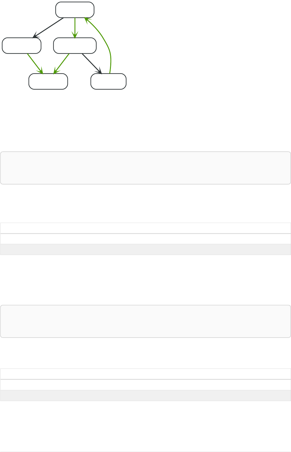
name = 'Anders'
name = 'Ceasar'
BLOCKS
name = 'Bossman'
KNOWS
name = 'George'
KNOWS
name = 'David'
BLOCKSKNOWS
KNOWS
Figure 11. Graph
3.5.2. Filter on aggregate function results
Aggregated results have to pass through a WITH clause to be able to filter on.
Query
MATCH (david { name: 'David' })--(otherPerson)-->()
WITH otherPerson, count(*) AS foaf
WHERE foaf > 1
RETURN otherPerson.name
The name of the person connected to 'David' with the at least more than one outgoing relationship
will be returned by the query.
Table 117. Result
otherPerson.name
"Anders"
1 row
3.5.3. Sort results before using collect on them
You can sort your results before passing them to collect, thus sorting the resulting list.
Query
MATCH (n)
WITH n
ORDER BY n.name DESC LIMIT 3
RETURN collect(n.name)
A list of the names of people in reverse order, limited to 3, is returned in a list.
Table 118. Result
collect(n.name)
["George","David","Ceasar"]
1 row
3.5.4. Limit branching of a path search
You can match paths, limit to a certain number, and then match again using those paths as a base, as
94

well as any number of similar limited searches.
Query
MATCH (n { name: 'Anders' })--(m)
WITH m
ORDER BY m.name DESC LIMIT 1
MATCH (m)--(o)
RETURN o.name
Starting at 'Anders', find all matching nodes, order by name descending and get the top result, then
find all the nodes connected to that top result, and return their names.
Table 119. Result
o.name
"Bossman"
"Anders"
2 rows
3.6. UNWIND
UNWIND expands a list into a sequence of rows.
•Introduction
•Unwinding a list
•Creating a distinct list
•Using UNWIND with any expression returning a list
•Using UNWIND with a list of lists
•Using UNWIND with an empty list
•Using UNWIND with an expression that is not a list
•Creating nodes from a list parameter
3.6.1. Introduction
With UNWIND, you can transform any list back into individual rows. These lists can be parameters that
were passed in, previously collect -ed result or other list expressions.
One common usage of unwind is to create distinct lists. Another is to create data from parameter lists
that are provided to the query.
UNWIND requires you to specify a new name for the inner values.
3.6.2. Unwinding a list
We want to transform the literal list into rows named x and return them.
Query
UNWIND [1, 2, 3, NULL ] AS x
RETURN x, 'val' AS y
95

Each value of the original list — including null — is returned as an individual row.
Table 120. Result
x y
1 "val"
2 "val"
3 "val"
<null> "val"
4 rows
3.6.3. Creating a distinct list
We want to transform a list of duplicates into a set using DISTINCT.
Query
WITH [1, 1, 2, 2] AS coll
UNWIND coll AS x
WITH DISTINCT x
RETURN collect(x) AS setOfVals
Each value of the original list is unwound and passed through DISTINCT to create a unique set.
Table 121. Result
setOfVals
[1,2]
1 row
3.6.4. Using UNWIND with any expression returning a list
Any expression that returns a list may be used with UNWIND.
Query
WITH [1, 2] AS a,[3, 4] AS b
UNWIND (a + b) AS x
RETURN x
The two lists — a and b — are concatenated to form a new list, which is then operated upon by UNWIND.
Table 122. Result
x
1
2
3
4
4 rows
96

3.6.5. Using UNWIND with a list of lists
Multiple UNWIND clauses can be chained to unwind nested list elements.
Query
WITH [[1, 2],[3, 4], 5] AS nested
UNWIND nested AS x
UNWIND x AS y
RETURN y
The first UNWIND results in three rows for x, each of which contains an element of the original list (two
of which are also lists); namely, [1, 2], [3, 4] and 5. The second UNWIND then operates on each of
these rows in turn, resulting in five rows for y.
Table 123. Result
y
1
2
3
4
5
5 rows
3.6.6. Using UNWIND with an empty list
Using an empty list with UNWIND will produce no rows, irrespective of whether or not any rows existed
beforehand, or whether or not other values are being projected.
Essentially, UNWIND [] reduces the number of rows to zero, and thus causes the query to cease its
execution, returning no results. This has value in cases such as UNWIND v, where v is a variable from an
earlier clause that may or may not be an empty list — when it is an empty list, this will behave just as a
MATCH that has no results.
Query
UNWIND [] AS empty
RETURN empty, 'literal_that_is_not_returned'
Table 124. Result
(empty result)
0 rows
To avoid inadvertently using UNWIND on an empty list, CASE may be used to replace an empty list with a
null:
WITH [] AS list
UNWIND
Ê CASE
Ê WHEN list = []
Ê THEN [null]
Ê ELSE list
Ê END AS emptylist
RETURN emptylist
97

3.6.7. Using UNWIND with an expression that is not a list
Attempting to use UNWIND on an expression that does not return a list — such as UNWIND 5 — will cause
an error. The exception to this is when the expression returns null — this will reduce the number of
rows to zero, causing it to cease its execution and return no results.
Query
UNWIND NULL AS x
RETURN x, 'some_literal'
Table 125. Result
(empty result)
0 rows
3.6.8. Creating nodes from a list parameter
Create a number of nodes and relationships from a parameter-list without using FOREACH.
Parameters
{
Ê "events" : [ {
Ê "year" : 2014,
Ê "id" : 1
Ê }, {
Ê "year" : 2014,
Ê "id" : 2
Ê } ]
}
Query
UNWIND $events AS event
MERGE (y:Year { year: event.year })
MERGE (y)<-[:IN]-(e:Event { id: event.id })
RETURN e.id AS x
ORDER BY x
Each value of the original list is unwound and passed through MERGE to find or create the nodes and
relationships.
Table 126. Result
x
1
2
2 rows
Nodes created: 3
Relationships created: 2
Properties set: 3
Labels added: 3
3.7. WHERE
WHERE adds constraints to the patterns in a MATCH or OPTIONAL MATCH clause or filters the
results of a WITH clause.
98

•Introduction
•Basic usage
•Boolean operations
•Filter on node label
•Filter on node property
•Filter on relationship property
•Filter on dynamically-computed property
•Property existence checking
•String matching
•Prefix string search using STARTS WITH
•Suffix string search using ENDS WITH
•Substring search using CONTAINS
•String matching negation
•Regular expressions
•Matching using regular expressions
•Escaping in regular expressions
•Case-insensitive regular expressions
•Using path patterns in WHERE
•Filter on patterns
•Filter on patterns using NOT
•Filter on patterns with properties
•Filter on relationship type
•Lists
•IN operator
•Missing properties and values
•Default to false if property is missing
•Default to true if property is missing
•Filter on null
•Using ranges
•Simple range
•Composite range
3.7.1. Introduction
WHERE is not a clause in its own right — rather, it’s part of MATCH, OPTIONAL MATCH, START and WITH.
In the case of WITH and START, WHERE simply filters the results.
For MATCH and OPTIONAL MATCH on the other hand, WHERE adds constraints to the patterns described. It
should not be seen as a filter after the matching is finished.
99
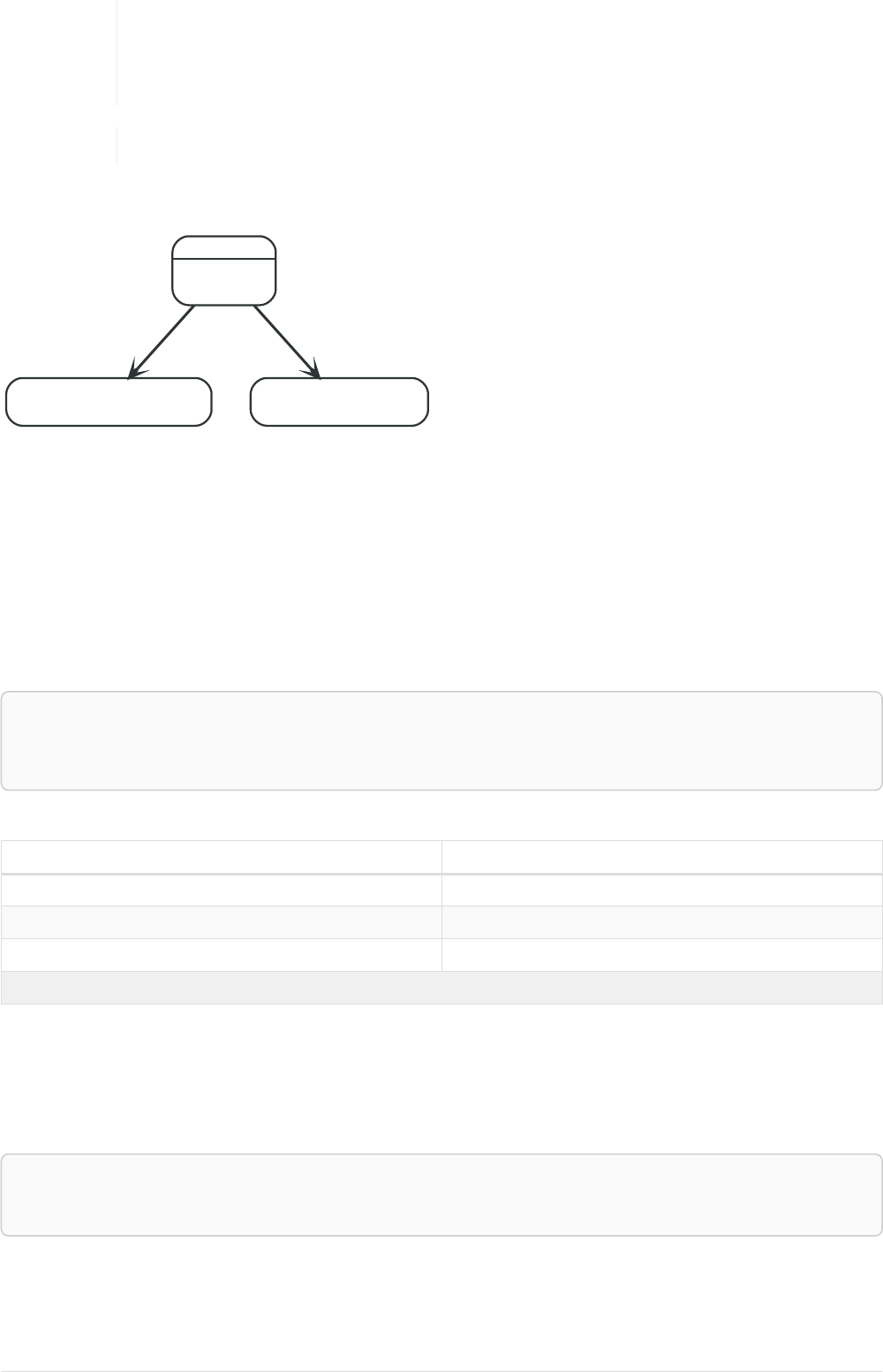
In the case of multiple MATCH / OPTIONAL MATCH clauses, the predicate in WHERE is
always a part of the patterns in the directly preceding MATCH / OPTIONAL MATCH. Both
results and performance may be impacted if the WHERE is put inside the wrong MATCH
clause.
Indexes` may be used to optimize queries using WHERE in a variety of cases.
The following graph is used for the examples below:
Swedish
belt = 'white'
name = 'Andy'
age = 36
email = 'peter_n@example.com'
name = 'Peter'
age = 35
KNOWS
since = 1999
address = 'Sweden/Malmo'
name = 'Timothy'
age = 25
KNOWS
since = 2012
Figure 12. Graph
3.7.2. Basic usage
Boolean operations
You can use the boolean operators AND, OR, XOR and NOT. See Working with null for more information
on how this works with null.
Query
MATCH (n)
WHERE n.name = 'Peter' XOR (n.age < 30 AND n.name = 'Timothy') OR NOT (n.name = 'Timothy' OR n.name =
'Peter')
RETURN n.name, n.age
Table 127. Result
n.name n.age
"Andy" 36
"Timothy" 25
"Peter" 35
3 rows
Filter on node label
To filter nodes by label, write a label predicate after the WHERE keyword using WHERE n:foo.
Query
MATCH (n)
WHERE n:Swedish
RETURN n.name, n.age
The name and age for the 'Andy' node will be returned.
Table 128. Result
100

n.name n.age
"Andy" 36
1 row
Filter on node property
To filter on a node property, write your clause after the WHERE keyword.
Query
MATCH (n)
WHERE n.age < 30
RETURN n.name, n.age
The name and age values for the 'Timothy' node are returned because he is less than 30 years of age.
Table 129. Result
n.name n.age
"Timothy" 25
1 row
Filter on relationship property
To filter on a relationship property, write your clause after the WHERE keyword.
Query
MATCH (n)-[k:KNOWS]->(f)
WHERE k.since < 2000
RETURN f.name, f.age, f.email
The name, age and email values for the 'Peter' node are returned because Andy has known him since
before 2000.
Table 130. Result
f.name f.age f.email
"Peter" 35 "peter_n@example.com"
1 row
Filter on dynamically-computed node property
To filter on a property using a dynamically computed name, use square bracket syntax.
Query
WITH 'AGE' AS propname
MATCH (n)
WHERE n[toLower(propname)]< 30
RETURN n.name, n.age
The name and age values for the 'Timothy' node are returned because he is less than 30 years of age.
Table 131. Result
101

n.name n.age
"Timothy" 25
1 row
Property existence checking
Use the exists() function to only include nodes or relationships in which a property exists.
Query
MATCH (n)
WHERE exists(n.belt)
RETURN n.name, n.belt
The name and belt for the 'Andy' node are returned because he is the only one with a belt property.
The has() function has been superseded by exists() and has been removed.
Table 132. Result
n.name n.belt
"Andy" "white"
1 row
3.7.3. String matching
The prefix and suffix of a string can be matched using STARTS WITH and ENDS WITH. To undertake a
substring search - i.e. match regardless of location within a string - use CONTAINS. The matching is case-
sensitive. Attempting to use these operators on values which are not strings will return null.
Prefix string search using STARTS WITH
The STARTS WITH operator is used to perform case-sensitive matching on the beginning of a string.
Query
MATCH (n)
WHERE n.name STARTS WITH 'Pet'
RETURN n.name, n.age
The name and age for the 'Peter' node are returned because his name starts with 'Pet'.
Table 133. Result
n.name n.age
"Peter" 35
1 row
Suffix string search using ENDS WITH
The ENDS WITH operator is used to perform case-sensitive matching on the ending of a string.
102

Query
MATCH (n)
WHERE n.name ENDS WITH 'ter'
RETURN n.name, n.age
The name and age for the 'Peter' node are returned because his name ends with 'ter'.
Table 134. Result
n.name n.age
"Peter" 35
1 row
Substring search using CONTAINS
The CONTAINS operator is used to perform case-sensitive matching regardless of location within a
string.
Query
MATCH (n)
WHERE n.name CONTAINS 'ete'
RETURN n.name, n.age
The name and age for the 'Peter' node are returned because his name contains with 'ete'.
Table 135. Result
n.name n.age
"Peter" 35
1 row
String matching negation
Use the NOT keyword to exclude all matches on given string from your result:
Query
MATCH (n)
WHERE NOT n.name ENDS WITH 'y'
RETURN n.name, n.age
The name and age for the 'Peter' node are returned because his name does not end with 'y'.
Table 136. Result
n.name n.age
"Peter" 35
1 row
3.7.4. Regular expressions
Cypher supports filtering using regular expressions. The regular expression syntax is inherited from
the Java regular expressions (https://docs.oracle.com/javase/7/docs/api/java/util/regex/Pattern.html). This
includes support for flags that change how strings are matched, including case-insensitive (?i),
103

multiline (?m) and dotall (?s). Flags are given at the beginning of the regular expression, for example
MATCH (n) WHERE n.name =~ '(?i)Lon.*' RETURN n will return nodes with name 'London' or with name
'LonDoN'.
Matching using regular expressions
You can match on regular expressions by using =~ 'regexp', like this:
Query
MATCH (n)
WHERE n.name =~ 'Tim.*'
RETURN n.name, n.age
The name and age for the 'Timothy' node are returned because his name starts with 'Tim'.
Table 137. Result
n.name n.age
"Timothy" 25
1 row
Escaping in regular expressions
Characters like . or * have special meaning in a regular expression. To use these as ordinary
characters, without special meaning, escape them.
Query
MATCH (n)
WHERE n.email =~ '.*\\.com'
RETURN n.name, n.age, n.email
The name, age and email for the 'Peter' node are returned because his email ends with '.com'.
Table 138. Result
n.name n.age n.email
"Peter" 35 "peter_n@example.com"
1 row
Case-insensitive regular expressions
By pre-pending a regular expression with (?i), the whole expression becomes case-insensitive.
Query
MATCH (n)
WHERE n.name =~ '(?i)AND.*'
RETURN n.name, n.age
The name and age for the 'Andy' node are returned because his name starts with 'AND' irrespective of
casing.
Table 139. Result
104

n.name n.age
"Andy" 36
1 row
3.7.5. Using path patterns in WHERE
Filter on patterns
Patterns are expressions in Cypher, expressions that return a list of paths. List expressions are also
predicates — an empty list represents false, and a non-empty represents true.
So, patterns are not only expressions, they are also predicates. The only limitation to your pattern is
that you must be able to express it in a single path. You cannot use commas between multiple paths
like you do in MATCH. You can achieve the same effect by combining multiple patterns with AND.
Note that you cannot introduce new variables here. Although it might look very similar to the MATCH
patterns, the WHERE clause is all about eliminating matched subgraphs. MATCH (a)-[]→(b) is very
different from WHERE (a)-[]→(b). The first will produce a subgraph for every path it can find between
a and b, whereas the latter will eliminate any matched subgraphs where a and b do not have a directed
relationship chain between them.
Query
MATCH (timothy { name: 'Timothy' }),(others)
WHERE others.name IN ['Andy', 'Peter'] AND (timothy)<--(others)
RETURN others.name, others.age
The name and age for nodes that have an outgoing relationship to the 'Timothy' node are returned.
Table 140. Result
others.name others.age
"Andy" 36
1 row
Filter on patterns using NOT
The NOT operator can be used to exclude a pattern.
Query
MATCH (persons),(peter { name: 'Peter' })
WHERE NOT (persons)-->(peter)
RETURN persons.name, persons.age
Name and age values for nodes that do not have an outgoing relationship to the 'Peter' node are
returned.
Table 141. Result
persons.name persons.age
"Timothy" 25
"Peter" 35
2 rows
105

Filter on patterns with properties
You can also add properties to your patterns:
Query
MATCH (n)
WHERE (n)-[:KNOWS]-({ name: 'Timothy' })
RETURN n.name, n.age
Finds all name and age values for nodes that have a KNOWS relationship to a node with the name
'Timothy'.
Table 142. Result
n.name n.age
"Andy" 36
1 row
Filter on relationship type
You can put the exact relationship type in the MATCH pattern, but sometimes you want to be able to do
more advanced filtering on the type. You can use the special property type to compare the type with
something else. In this example, the query does a regular expression comparison with the name of
the relationship type.
Query
MATCH (n)-[r]->()
WHERE n.name='Andy' AND type(r)=~ 'K.*'
RETURN type(r), r.since
This returns all relationships having a type whose name starts with 'K'.
Table 143. Result
type(r) r.since
"KNOWS" 1999
"KNOWS" 2012
2 rows
3.7.6. Lists
IN operator
To check if an element exists in a list, you can use the IN operator.
Query
MATCH (a)
WHERE a.name IN ['Peter', 'Timothy']
RETURN a.name, a.age
This query shows how to check if a property exists in a literal list.
Table 144. Result
106

a.name a.age
"Timothy" 25
"Peter" 35
2 rows
3.7.7. Missing properties and values
Default to false if property is missing
As missing properties evaluate to null, the comparison in the example will evaluate to false for nodes
without the belt property.
Query
MATCH (n)
WHERE n.belt = 'white'
RETURN n.name, n.age, n.belt
Only the name, age and belt values of nodes with white belts are returned.
Table 145. Result
n.name n.age n.belt
"Andy" 36 "white"
1 row
Default to true if property is missing
If you want to compare a property on a node or relationship, but only if it exists, you can compare the
property against both the value you are looking for and null, like:
Query
MATCH (n)
WHERE n.belt = 'white' OR n.belt IS NULL RETURN n.name, n.age, n.belt
ORDER BY n.name
This returns all values for all nodes, even those without the belt property.
Table 146. Result
n.name n.age n.belt
"Andy" 36 "white"
"Peter" 35 <null>
"Timothy" 25 <null>
3 rows
Filter on null
Sometimes you might want to test if a value or a variable is null. This is done just like SQL does it,
using IS NULL. Also like SQL, the negative is IS NOT NULL, although NOT(IS NULL x) also works.
107

Query
MATCH (person)
WHERE person.name = 'Peter' AND person.belt IS NULL RETURN person.name, person.age, person.belt
The name and age values for nodes that have name 'Peter' but no belt property are returned.
Table 147. Result
person.name person.age person.belt
"Peter" 35 <null>
1 row
3.7.8. Using ranges
Simple range
To check for an element being inside a specific range, use the inequality operators <, <=, >=, >.
Query
MATCH (a)
WHERE a.name >= 'Peter'
RETURN a.name, a.age
The name and age values of nodes having a name property lexicographically greater than or equal to
'Peter' are returned.
Table 148. Result
a.name a.age
"Timothy" 25
"Peter" 35
2 rows
Composite range
Several inequalities can be used to construct a range.
Query
MATCH (a)
WHERE a.name > 'Andy' AND a.name < 'Timothy'
RETURN a.name, a.age
The name and age values of nodes having a name property lexicographically between 'Andy' and
'Timothy' are returned.
Table 149. Result
a.name a.age
"Peter" 35
1 row
108
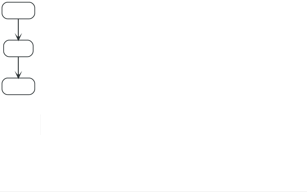
3.8. ORDER BY
ORDER BY is a sub-clause following RETURN or WITH, and it specifies that the output should be
sorted and how.
•Introduction
•Order nodes by property
•Order nodes by multiple properties
•Order nodes in descending order
•Ordering null
3.8.1. Introduction
Note that you cannot sort on nodes or relationships, just on properties on these. ORDER BY relies on
comparisons to sort the output, see Ordering and comparison of values.
In terms of scope of variables, ORDER BY follows special rules, depending on if the projecting RETURN or
WITH clause is either aggregating or DISTINCT. If it is an aggregating or DISTINCT projection, only
the variables available in the projection are available. If the projection does not alter the output
cardinality (which aggregation and DISTINCT do), variables available from before the projecting clause
are also available. When the projection clause shadows already existing variables, only the new
variables are available.
Lastly, it is not allowed to use aggregating expressions in the ORDER BY sub-clause if they are not also
listed in the projecting clause. This last rule is to make sure that ORDER BY does not change the
results, only the order of them.
The performance of Cypher queries using ORDER BY on node properties can be influenced by the
existence and use of an index for finding the nodes. If the index can provide the nodes in the order
requested in the query, Cypher can avoid the use of an expensive Sort operation. Read more about
this capability in the section on Index Values and Order.
name = 'A'
length = 170
age = 34
name = 'B'
age = 34
KNOWS
name = 'C'
length = 185
age = 32
KNOWS
Figure 13. Graph
Strings that contain special characters can have inconsistent or non-deterministic
ordering in Neo4j. For details, see Sorting of special characters.
3.8.2. Order nodes by property
ORDER BY is used to sort the output.
109

Query
MATCH (n)
RETURN n.name, n.age
ORDER BY n.name
The nodes are returned, sorted by their name.
Table 150. Result
n.name n.age
"A" 34
"B" 34
"C" 32
3 rows
3.8.3. Order nodes by multiple properties
You can order by multiple properties by stating each variable in the ORDER BY clause. Cypher will sort
the result by the first variable listed, and for equals values, go to the next property in the ORDER BY
clause, and so on.
Query
MATCH (n)
RETURN n.name, n.age
ORDER BY n.age, n.name
This returns the nodes, sorted first by their age, and then by their name.
Table 151. Result
n.name n.age
"C" 32
"A" 34
"B" 34
3 rows
3.8.4. Order nodes in descending order
By adding DESC[ENDING] after the variable to sort on, the sort will be done in reverse order.
Query
MATCH (n)
RETURN n.name, n.age
ORDER BY n.name DESC
The example returns the nodes, sorted by their name in reverse order.
Table 152. Result
n.name n.age
"C" 32
"B" 34
110

n.name n.age
"A" 34
3 rows
3.8.5. Ordering null
When sorting the result set, null will always come at the end of the result set for ascending sorting,
and first when doing descending sort.
Query
MATCH (n)
RETURN n.length, n.name, n.age
ORDER BY n.length
The nodes are returned sorted by the length property, with a node without that property last.
Table 153. Result
n.length n.name n.age
170 "A" 34
185 "C" 32
<null> "B" 34
3 rows
3.9. SKIP
SKIP defines from which row to start including the rows in the output.
•Introduction
•Skip first three rows
•Return middle two rows
•Using an expression with SKIP to return a subset of the rows
3.9.1. Introduction
By using SKIP, the result set will get trimmed from the top. Please note that no guarantees are made
on the order of the result unless the query specifies the ORDER BY clause. SKIP accepts any expression
that evaluates to a positive integer — however the expression cannot refer to nodes or relationships.
name = 'A'
name = 'E'
KNOWS
name = 'D'
KNOWS
name = 'C'
KNOWS
name = 'B'
KNOWS
Figure 14. Graph
111

3.9.2. Skip first three rows
To return a subset of the result, starting from the fourth result, use the following syntax:
Query
MATCH (n)
RETURN n.name
ORDER BY n.name
SKIP 3
The first three nodes are skipped, and only the last two are returned in the result.
Table 154. Result
n.name
"D"
"E"
2 rows
3.9.3. Return middle two rows
To return a subset of the result, starting from somewhere in the middle, use this syntax:
Query
MATCH (n)
RETURN n.name
ORDER BY n.name
SKIP 1
LIMIT 2
Two nodes from the middle are returned.
Table 155. Result
n.name
"B"
"C"
2 rows
3.9.4. Using an expression with SKIP to return a subset of the rows
Skip accepts any expression that evaluates to a positive integer as long as it is not referring to any
external variables:
Query
MATCH (n)
RETURN n.name
ORDER BY n.name
SKIP toInteger(3*rand())+ 1
The first three nodes are skipped, and only the last two are returned in the result.
Table 156. Result
112
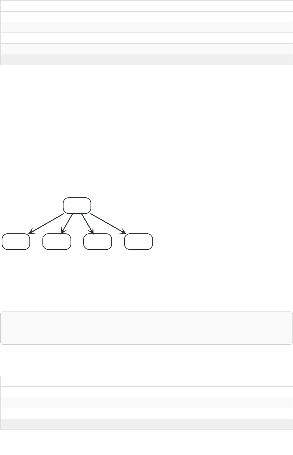
n.name
"B"
"C"
"D"
"E"
4 rows
3.10. LIMIT
LIMIT constrains the number of rows in the output.
•Introduction
•Return a subset of the rows
•Using an expression with LIMIT to return a subset of the rows
3.10.1. Introduction
LIMIT accepts any expression that evaluates to a positive integer — however the expression cannot
refer to nodes or relationships.
name = 'A'
name = 'E'
KNOWS
name = 'D'
KNOWS
name = 'C'
KNOWS
name = 'B'
KNOWS
Figure 15. Graph
3.10.2. Return a subset of the rows
To return a subset of the result, starting from the top, use this syntax:
Query
MATCH (n)
RETURN n.name
ORDER BY n.name
LIMIT 3
The top three items are returned by the example query.
Table 157. Result
n.name
"A"
"B"
"C"
3 rows
113

3.10.3. Using an expression with LIMIT to return a subset of the rows
Limit accepts any expression that evaluates to a positive integer as long as it is not referring to any
external variables:
Query
MATCH (n)
RETURN n.name
ORDER BY n.name
LIMIT toInteger(3 * rand())+ 1
Returns one to three top items.
Table 158. Result
n.name
"A"
"B"
2 rows
3.11. CREATE
The CREATE clause is used to create nodes and relationships.
•Create nodes
•Create single node
•Create multiple nodes
•Create a node with a label
•Create a node with multiple labels
•Create node and add labels and properties
•Return created node
•Create relationships
•Create a relationship between two nodes
•Create a relationship and set properties
•Create a full path
•Use parameters with CREATE
•Create node with a parameter for the properties
•Create multiple nodes with a parameter for their properties
In the CREATE clause, patterns are used extensively. Read Patterns for an
introduction.
3.11.1. Create nodes
114

Create single node
Creating a single node is done by issuing the following query:
Query
CREATE (n)
Nothing is returned from this query, except the count of affected nodes.
Table 159. Result
(empty result)
0 rows
Nodes created: 1
Create multiple nodes
Creating multiple nodes is done by separating them with a comma.
Query
CREATE (n),(m)
Table 160. Result
(empty result)
0 rows
Nodes created: 2
Create a node with a label
To add a label when creating a node, use the syntax below:
Query
CREATE (n:Person)
Nothing is returned from this query.
Table 161. Result
(empty result)
0 rows
Nodes created: 1
Labels added: 1
Create a node with multiple labels
To add labels when creating a node, use the syntax below. In this case, we add two labels.
Query
CREATE (n:Person:Swedish)
Nothing is returned from this query.
115

Table 162. Result
(empty result)
0 rows
Nodes created: 1
Labels added: 2
Create node and add labels and properties
When creating a new node with labels, you can add properties at the same time.
Query
CREATE (n:Person { name: 'Andy', title: 'Developer' })
Nothing is returned from this query.
Table 163. Result
(empty result)
0 rows
Nodes created: 1
Properties set: 2
Labels added: 1
Return created node
Creating a single node is done by issuing the following query:
Query
CREATE (a { name: 'Andy' })
RETURN a.name
The newly-created node is returned.
Table 164. Result
a.name
"Andy"
1 row
Nodes created: 1
Properties set: 1
3.11.2. Create relationships
Create a relationship between two nodes
To create a relationship between two nodes, we first get the two nodes. Once the nodes are loaded,
we simply create a relationship between them.
Query
MATCH (a:Person),(b:Person)
WHERE a.name = 'A' AND b.name = 'B'
CREATE (a)-[r:RELTYPE]->(b)
RETURN type(r)
116

The created relationship is returned by the query.
Table 165. Result
type(r)
"RELTYPE"
1 row
Relationships created: 1
Create a relationship and set properties
Setting properties on relationships is done in a similar manner to how it’s done when creating nodes.
Note that the values can be any expression.
Query
MATCH (a:Person),(b:Person)
WHERE a.name = 'A' AND b.name = 'B'
CREATE (a)-[r:RELTYPE { name: a.name + '<->' + b.name }]->(b)
RETURN type(r), r.name
The newly-created relationship is returned by the example query.
Table 166. Result
type(r) r.name
"RELTYPE" "A<->B"
1 row
Relationships created: 1
Properties set: 1
3.11.3. Create a full path
When you use CREATE and a pattern, all parts of the pattern that are not already in scope at this time
will be created.
Query
CREATE p =(andy { name:'Andy' })-[:WORKS_AT]->(neo)<-[:WORKS_AT]-(michael { name: 'Michael' })
RETURN p
This query creates three nodes and two relationships in one go, assigns it to a path variable, and
returns it.
Table 167. Result
p
(20)-[WORKS_AT,0]->(21)<-[WORKS_AT,1]-(22)
1 row
Nodes created: 3
Relationships created: 2
Properties set: 2
3.11.4. Use parameters with CREATE
117

Create node with a parameter for the properties
You can also create a graph entity from a map. All the key/value pairs in the map will be set as
properties on the created relationship or node. In this case we add a Person label to the node as well.
Parameters
{
Ê "props" : {
Ê "name" : "Andy",
Ê "position" : "Developer"
Ê }
}
Query
CREATE (n:Person $props)
RETURN n
Table 168. Result
n
Node[20]{name:"Andy",position:"Developer"}
1 row
Nodes created: 1
Properties set: 2
Labels added: 1
Create multiple nodes with a parameter for their properties
By providing Cypher an array of maps, it will create a node for each map.
Parameters
{
Ê "props" : [ {
Ê "name" : "Andy",
Ê "position" : "Developer"
Ê }, {
Ê "name" : "Michael",
Ê "position" : "Developer"
Ê } ]
}
Query
UNWIND $props AS map
CREATE (n)
SET n = map
Table 169. Result
(empty result)
0 rows
Nodes created: 2
Properties set: 4
3.12. DELETE
The DELETE clause is used to delete nodes, relationships or paths.
118
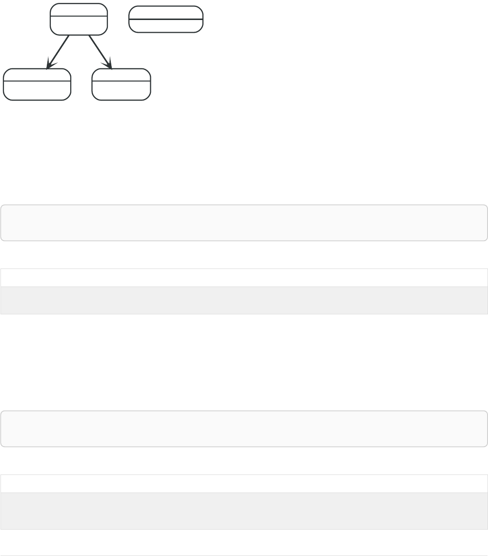
•Introduction
•Delete a single node
•Delete all nodes and relationships
•Delete a node with all its relationships
•Delete relationships only
3.12.1. Introduction
For removing properties and labels, see REMOVE. Remember that you cannot delete a node without
also deleting relationships that start or end on said node. Either explicitly delete the relationships, or
use DETACH DELETE.
The examples start out with the following database:
Person
name = 'Andy'
age = 36
Person
name = 'Timothy'
age = 25
KNOWS
Person
name = 'Peter'
age = 34
KNOWS
Person
name = 'UNKNOWN'
Figure 16. Graph
3.12.2. Delete single node
To delete a node, use the DELETE clause.
Query
MATCH (n:Person { name: 'UNKNOWN' })
DELETE n
Table 170. Result
(empty result)
0 rows
Nodes deleted: 1
3.12.3. Delete all nodes and relationships
This query isn’t for deleting large amounts of data, but is useful when experimenting with small
example data sets.
Query
MATCH (n)
DETACH DELETE n
Table 171. Result
(empty result)
0 rows
Nodes deleted: 4
Relationships deleted: 2
119

3.12.4. Delete a node with all its relationships
When you want to delete a node and any relationship going to or from it, use DETACH DELETE.
Query
MATCH (n { name: 'Andy' })
DETACH DELETE n
Table 172. Result
(empty result)
0 rows
Nodes deleted: 1
Relationships deleted: 2
3.12.5. Delete relationships only
It is also possible to delete relationships only, leaving the node(s) otherwise unaffected.
Query
MATCH (n { name: 'Andy' })-[r:KNOWS]->()
DELETE r
This deletes all outgoing KNOWS relationships from the node with the name 'Andy'.
Table 173. Result
(empty result)
0 rows
Relationships deleted: 2
3.13. SET
The SET clause is used to update labels on nodes and properties on nodes and relationships.
•Introduction
•Set a property
•Update a property
•Remove a property
•Copy properties between nodes and relationships
•Replace all properties using a map and =
•Remove all properties using an empty map and =
•Mutate specific properties using a map and +=
•Set multiple properties using one SET clause
•Set a property using a parameter
•Set all properties using a parameter
•Set a label on a node
•Set multiple labels on a node
120
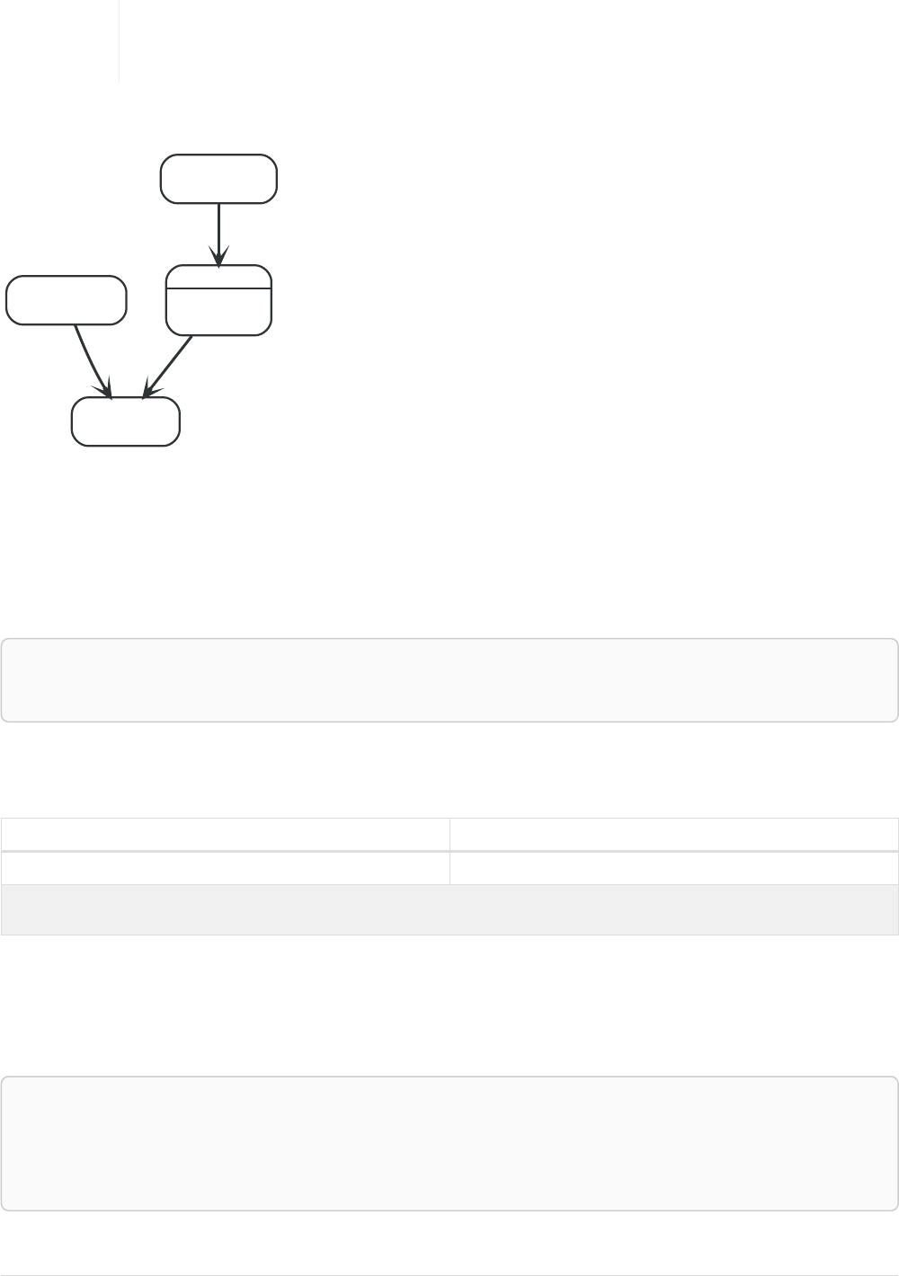
3.13.1. Introduction
SET can be used with a map — provided as a literal, a parameter, or a node or relationship — to set
properties.
Setting labels on a node is an idempotent operation — nothing will occur if an
attempt is made to set a label on a node that already has that label. The query
statistics will state whether any updates actually took place.
The examples use this graph as a starting point:
Swedish
hungry = true
name = 'Andy'
age = 36
name = 'Peter'
age = 34
KNOWS
name = 'Stefan'
KNOWS
name = 'George'
KNOWS
Figure 17. Graph
3.13.2. Set a property
Use SET to set a property on a node or relationship:
Query
MATCH (n { name: 'Andy' })
SET n.surname = 'Taylor'
RETURN n.name, n.surname
The newly-changed node is returned by the query.
Table 174. Result
n.name n.surname
"Andy" "Taylor"
1 row
Properties set: 1
It is possible to set a property on a node or relationship using more complex expressions. For
instance, in contrast to specifying the node directly, the following query shows how to set a property
for a node selected by an expression:
Query
MATCH (n { name: 'Andy' })
SET (
CASE
WHEN n.age = 36
THEN n END ).worksIn = 'Malmo'
RETURN n.name, n.worksIn
121

Table 175. Result
n.name n.worksIn
"Andy" "Malmo"
1 row
Properties set: 1
No action will be taken if the node expression evaluates to null, as shown in this example:
Query
MATCH (n { name: 'Andy' })
SET (
CASE
WHEN n.age = 55
THEN n END ).worksIn = 'Malmo'
RETURN n.name, n.worksIn
As no node matches the CASE expression, the expression returns a null. As a consequence, no
updates occur, and therefore no worksIn property is set.
Table 176. Result
n.name n.worksIn
"Andy" <null>
1 row
3.13.3. Update a property
SET can be used to update a property on a node or relationship. This query forces a change of type in
the age property:
Query
MATCH (n { name: 'Andy' })
SET n.age = toString(n.age)
RETURN n.name, n.age
The age property has been converted to the string '36'.
Table 177. Result
n.name n.age
"Andy" "36"
1 row
Properties set: 1
3.13.4. Remove a property
Although REMOVE is normally used to remove a property, it’s sometimes convenient to do it using the
SET command. A case in point is if the property is provided by a parameter.
Query
MATCH (n { name: 'Andy' })
SET n.name = NULL RETURN n.name, n.age
122

The name property is now missing.
Table 178. Result
n.name n.age
<null> 36
1 row
Properties set: 1
3.13.5. Copy properties between nodes and relationships
SET can be used to copy all properties from one node or relationship to another. This will remove all
other properties on the node or relationship being copied to.
Query
MATCH (at { name: 'Andy' }),(pn { name: 'Peter' })
SET at = pn
RETURN at.name, at.age, at.hungry, pn.name, pn.age
The 'Andy' node has had all its properties replaced by the properties of the 'Peter' node.
Table 179. Result
at.name at.age at.hungry pn.name pn.age
"Peter" 34 <null> "Peter" 34
1 row
Properties set: 3
3.13.6. Replace all properties using a map and =
The property replacement operator = can be used with SET to replace all existing properties on a node
or relationship with those provided by a map:
Query
MATCH (p { name: 'Peter' })
SET p = { name: 'Peter Smith', position: 'Entrepreneur' }
RETURN p.name, p.age, p.position
This query updated the name property from Peter to Peter Smith, deleted the age property, and added
the position property to the 'Peter' node.
Table 180. Result
p.name p.age p.position
"Peter Smith" <null> "Entrepreneur"
1 row
Properties set: 3
3.13.7. Remove all properties using an empty map and =
All existing properties can be removed from a node or relationship by using SET with = and an empty
map as the right operand:
123

Query
MATCH (p { name: 'Peter' })
SET p = { }
RETURN p.name, p.age
This query removed all the existing properties — namely, name and age — from the 'Peter' node.
Table 181. Result
p.name p.age
<null> <null>
1 row
Properties set: 2
3.13.8. Mutate specific properties using a map and +=
The property mutation operator += can be used with SET to mutate properties from a map in a fine-
grained fashion:
•Any properties in the map that are not on the node or relationship will be added.
•Any properties not in the map that are on the node or relationship will be left as is.
•Any properties that are in both the map and the node or relationship will be replaced in the node
or relationship. However, if any property in the map is null, it will be removed from the node or
relationship.
Query
MATCH (p { name: 'Peter' })
SET p += { age: 38, hungry: TRUE , position: 'Entrepreneur' }
RETURN p.name, p.age, p.hungry, p.position
This query left the name property unchanged, updated the age property from 34 to 38, and added the
hungry and position properties to the 'Peter' node.
Table 182. Result
p.name p.age p.hungry p.position
"Peter" 38 true "Entrepreneur"
1 row
Properties set: 3
In contrast to the property replacement operator =, providing an empty map as the right operand to
+= will not remove any existing properties from a node or relationship. In line with the semantics
detailed above, passing in an empty map with += will have no effect:
Query
MATCH (p { name: 'Peter' })
SET p += { }
RETURN p.name, p.age
Table 183. Result
p.name p.age
"Peter" 34
124

p.name p.age
1 row
3.13.9. Set multiple properties using one SET clause
Set multiple properties at once by separating them with a comma:
Query
MATCH (n { name: 'Andy' })
SET n.position = 'Developer', n.surname = 'Taylor'
Table 184. Result
(empty result)
0 rows
Properties set: 2
3.13.10. Set a property using a parameter
Use a parameter to set the value of a property:
Parameters
{
Ê "surname" : "Taylor"
}
Query
MATCH (n { name: 'Andy' })
SET n.surname = $surname
RETURN n.name, n.surname
A surname property has been added to the 'Andy' node.
Table 185. Result
n.name n.surname
"Andy" "Taylor"
1 row
Properties set: 1
3.13.11. Set all properties using a parameter
This will replace all existing properties on the node with the new set provided by the parameter.
Parameters
{
Ê "props" : {
Ê "name" : "Andy",
Ê "position" : "Developer"
Ê }
}
125

Query
MATCH (n { name: 'Andy' })
SET n = $props
RETURN n.name, n.position, n.age, n.hungry
The 'Andy' node has had all its properties replaced by the properties in the props parameter.
Table 186. Result
n.name n.position n.age n.hungry
"Andy" "Developer" <null> <null>
1 row
Properties set: 4
3.13.12. Set a label on a node
Use SET to set a label on a node:
Query
MATCH (n { name: 'Stefan' })
SET n:German
RETURN n.name, labels(n) AS labels
The newly-labeled node is returned by the query.
Table 187. Result
n.name labels
"Stefan" ["German"]
1 row
Labels added: 1
3.13.13. Set multiple labels on a node
Set multiple labels on a node with SET and use : to separate the different labels:
Query
MATCH (n { name: 'George' })
SET n:Swedish:Bossman
RETURN n.name, labels(n) AS labels
The newly-labeled node is returned by the query.
Table 188. Result
n.name labels
"George" ["Swedish","Bossman"]
1 row
Labels added: 2
3.14. REMOVE
The REMOVE clause is used to remove properties from nodes and relationships, and to remove
126
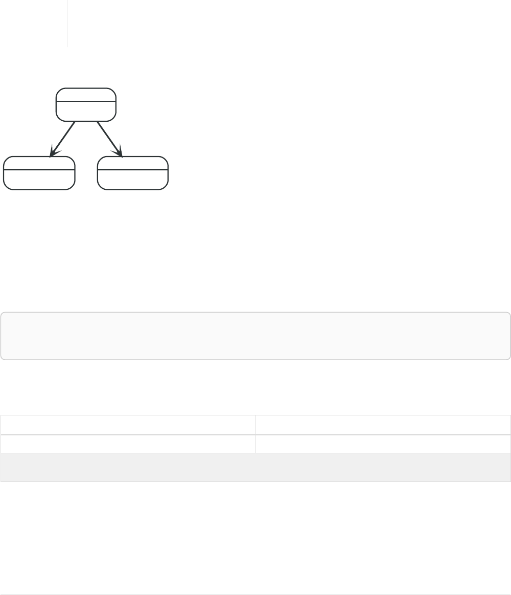
labels from nodes.
•Introduction
•Remove a property
•Remove all properties
•Remove a label from a node
•Remove multiple labels from a node
3.14.1. Introduction
For deleting nodes and relationships, see DELETE.
Removing labels from a node is an idempotent operation: if you try to remove a
label from a node that does not have that label on it, nothing happens. The query
statistics will tell you if something needed to be done or not.
The examples use the following database:
Swedish
name = 'Andy'
age = 36
Swedish, German
name = 'Peter'
age = 34
KNOWS
Swedish
name = 'Timothy'
age = 25
KNOWS
Figure 18. Graph
3.14.2. Remove a property
Neo4j doesn’t allow storing null in properties. Instead, if no value exists, the property is just not there.
So, REMOVE is used to remove a property value from a node or a relationship.
Query
MATCH (a { name: 'Andy' })
REMOVE a.age
RETURN a.name, a.age
The node is returned, and no property age exists on it.
Table 189. Result
a.name a.age
"Andy" <null>
1 row
Properties set: 1
3.14.3. Remove all properties
REMOVE cannot be used to remove all existing properties from a node or relationship. Instead, using SET
with = and an empty map as the right operand will clear all properties from the node or relationship.
127

3.14.4. Remove a label from a node
To remove labels, you use REMOVE.
Query
MATCH (n { name: 'Peter' })
REMOVE n:German
RETURN n.name, labels(n)
Table 190. Result
n.name labels(n)
"Peter" ["Swedish"]
1 row
Labels removed: 1
3.14.5. Remove multiple labels from a node
To remove multiple labels, you use REMOVE.
Query
MATCH (n { name: 'Peter' })
REMOVE n:German:Swedish
RETURN n.name, labels(n)
Table 191. Result
n.name labels(n)
"Peter" []
1 row
Labels removed: 2
3.15. FOREACH
The FOREACH clause is used to update data within a list, whether components of a path, or
result of aggregation.
•Introduction
•Mark all nodes along a path
3.15.1. Introduction
Lists and paths are key concepts in Cypher. FOREACH can be used to update data, such as executing
update commands on elements in a path, or on a list created by aggregation.
The variable context within the FOREACH parenthesis is separate from the one outside it. This means
that if you CREATE a node variable within a FOREACH, you will not be able to use it outside of the foreach
statement, unless you match to find it.
Within the FOREACH parentheses, you can do any of the updating commands — CREATE, CREATE UNIQUE,
MERGE, DELETE, and FOREACH.
128
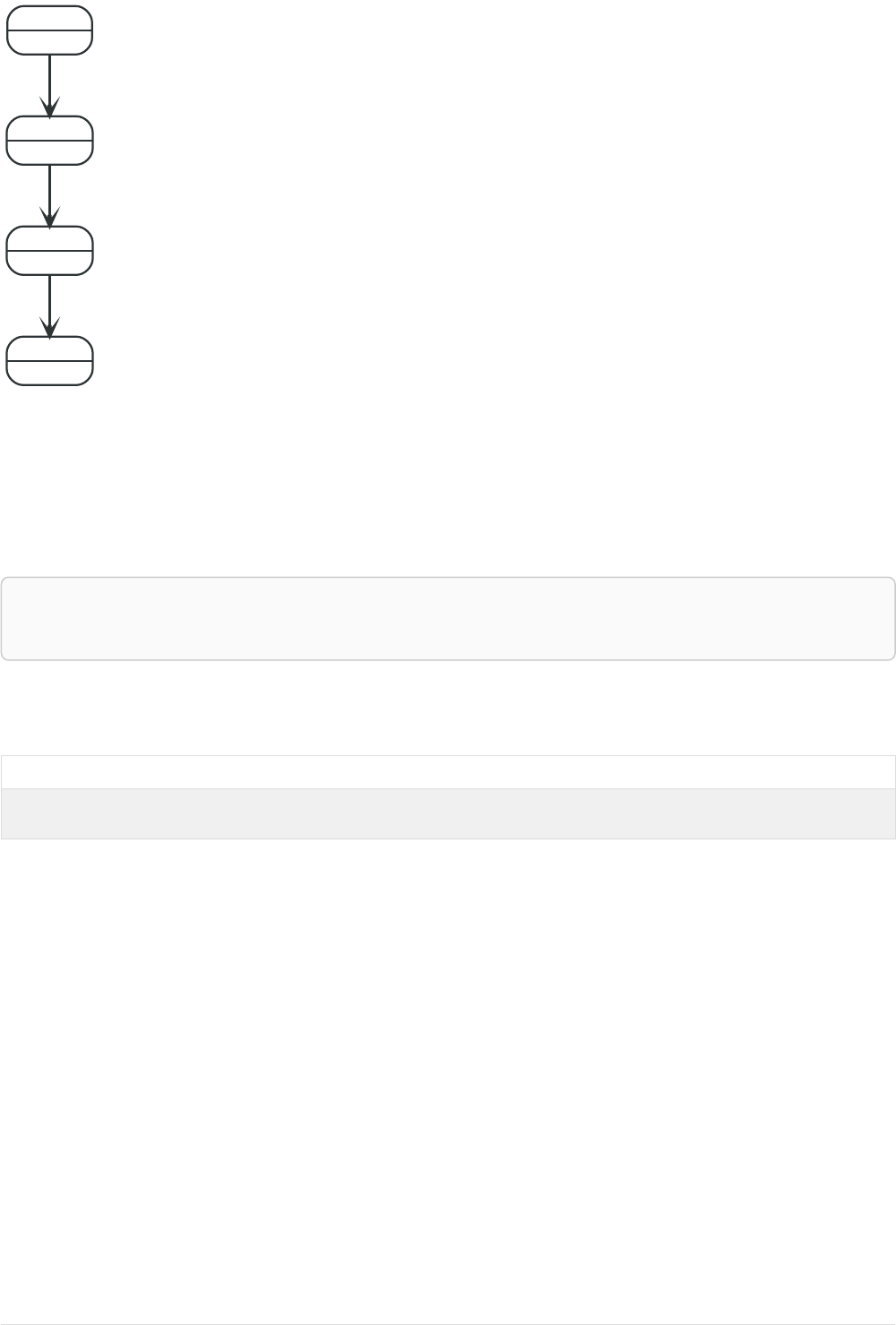
If you want to execute an additional MATCH for each element in a list then UNWIND (see UNWIND) would
be a more appropriate command.
Person
name = 'A'
Person
name = 'B'
KNOWS
Person
name = 'C'
KNOWS
Person
name = 'D'
KNOWS
Figure 19. Graph
3.15.2. Mark all nodes along a path
This query will set the property marked to true on all nodes along a path.
Query
MATCH p =(begin)-[*]->(END )
WHERE begin.name = 'A' AND END .name = 'D'
FOREACH (n IN nodes(p)| SET n.marked = TRUE )
Nothing is returned from this query, but four properties are set.
Table 192. Result
(empty result)
0 rows
Properties set: 4
3.16. MERGE
The MERGE clause ensures that a pattern exists in the graph. Either the pattern already exists,
or it needs to be created.
•Introduction
•Merge nodes
•Merge single node with a label
•Merge single node with properties
•Merge single node specifying both label and property
•Merge single node derived from an existing node property
•Use ON CREATE and ON MATCH
129

•Merge with ON CREATE
•Merge with ON MATCH
•Merge with ON CREATE and ON MATCH
•Merge with ON MATCH setting multiple properties
•Merge relationships
•Merge on a relationship
•Merge on multiple relationships
•Merge on an undirected relationship
•Merge on a relationship between two existing nodes
•Merge on a relationship between an existing node and a merged node derived from a node
property
•Using unique constraints with MERGE
•Merge using unique constraints creates a new node if no node is found
•Merge using unique constraints matches an existing node
•Merge with unique constraints and partial matches
•Merge with unique constraints and conflicting matches
•Using map parameters with MERGE
3.16.1. Introduction
MERGE either matches existing nodes and binds them, or it creates new data and binds that. It’s like a
combination of MATCH and CREATE that additionally allows you to specify what happens if the data was
matched or created.
For example, you can specify that the graph must contain a node for a user with a certain name. If
there isn’t a node with the correct name, a new node will be created and its name property set.
When using MERGE on full patterns, the behavior is that either the whole pattern matches, or the whole
pattern is created. MERGE will not partially use existing patterns — it’s all or nothing. If partial matches
are needed, this can be accomplished by splitting a pattern up into multiple MERGE clauses.
As with MATCH, MERGE can match multiple occurrences of a pattern. If there are multiple matches, they
will all be passed on to later stages of the query.
The last part of MERGE is the ON CREATE and ON MATCH. These allow a query to express additional changes
to the properties of a node or relationship, depending on if the element was MATCH -ed in the database
or if it was CREATE -ed.
The following graph is used for the examples below:
130

Person
chauffeurName = 'John Brown'
name = 'Charlie Sheen'
bornIn = 'New York'
Person
chauffeurName = 'Bob Brown'
name = 'Martin Sheen'
bornIn = 'Ohio'
FATHER
Movie
title = 'Wall Street'
ACTED_IN
ACTED_IN
Movie
title = 'The American President'
ACTED_IN
Person
bornIn = 'New Jersey'
chauffeurName = 'John Brown'
name = 'Michael Douglas'
ACTED_IN ACTED_IN
Person
chauffeurName = 'Bill White'
name = 'Oliver Stone'
bornIn = 'New York'
ACTED_IN
Person
chauffeurName = 'Ted Green'
name = 'Rob Reiner'
bornIn = 'New York'
ACTED_IN
Figure 20. Graph
3.16.2. Merge nodes
Merge single node with a label
Merging a single node with the given label.
Query
MERGE (robert:Critic)
RETURN robert, labels(robert)
A new node is created because there are no nodes labeled Critic in the database.
Table 193. Result
robert labels(robert)
Node[20]{} ["Critic"]
1 row
Nodes created: 1
Labels added: 1
Merge single node with properties
Merging a single node with properties where not all properties match any existing node.
Query
MERGE (charlie { name: 'Charlie Sheen', age: 10 })
RETURN charlie
A new node with the name 'Charlie Sheen' will be created since not all properties matched the
existing 'Charlie Sheen' node.
Table 194. Result
charlie
Node[20]{name:"Charlie Sheen",age:10}
1 row
Nodes created: 1
Properties set: 2
Merge single node specifying both label and property
Merging a single node with both label and property matching an existing node.
131

Query
MERGE (michael:Person { name: 'Michael Douglas' })
RETURN michael.name, michael.bornIn
'Michael Douglas' will be matched and the name and bornIn properties returned.
Table 195. Result
michael.name michael.bornIn
"Michael Douglas" "New Jersey"
1 row
Merge single node derived from an existing node property
For some property 'p' in each bound node in a set of nodes, a single new node is created for each
unique value for 'p'.
Query
MATCH (person:Person)
MERGE (city:City { name: person.bornIn })
RETURN person.name, person.bornIn, city
Three nodes labeled City are created, each of which contains a name property with the value of 'New
York', 'Ohio', and 'New Jersey', respectively. Note that even though the MATCH clause results in three
bound nodes having the value 'New York' for the bornIn property, only a single 'New York' node (i.e. a
City node with a name of 'New York') is created. As the 'New York' node is not matched for the first
bound node, it is created. However, the newly-created 'New York' node is matched and bound for the
second and third bound nodes."
Table 196. Result
person.name person.bornIn city
"Charlie Sheen" "New York" Node[20]{name:"New York"}
"Martin Sheen" "Ohio" Node[21]{name:"Ohio"}
"Michael Douglas" "New Jersey" Node[22]{name:"New Jersey"}
"Oliver Stone" "New York" Node[20]{name:"New York"}
"Rob Reiner" "New York" Node[20]{name:"New York"}
5 rows
Nodes created: 3
Properties set: 3
Labels added: 3
3.16.3. Use ON CREATE and ON MATCH
Merge with ON CREATE
Merge a node and set properties if the node needs to be created.
Query
MERGE (keanu:Person { name: 'Keanu Reeves' })
ON CREATE SET keanu.created = timestamp()
RETURN keanu.name, keanu.created
132

The query creates the 'keanu' node and sets a timestamp on creation time.
Table 197. Result
keanu.name keanu.created
"Keanu Reeves" 1544445306860
1 row
Nodes created: 1
Properties set: 2
Labels added: 1
Merge with ON MATCH
Merging nodes and setting properties on found nodes.
Query
MERGE (person:Person)
ON MATCH SET person.found = TRUE RETURN person.name, person.found
The query finds all the Person nodes, sets a property on them, and returns them.
Table 198. Result
person.name person.found
"Charlie Sheen" true
"Martin Sheen" true
"Michael Douglas" true
"Oliver Stone" true
"Rob Reiner" true
5 rows
Properties set: 5
Merge with ON CREATE and ON MATCH
Query
MERGE (keanu:Person { name: 'Keanu Reeves' })
ON CREATE SET keanu.created = timestamp()
ON MATCH SET keanu.lastSeen = timestamp()
RETURN keanu.name, keanu.created, keanu.lastSeen
The query creates the 'keanu' node, and sets a timestamp on creation time. If 'keanu' had already
existed, a different property would have been set.
Table 199. Result
keanu.name keanu.created keanu.lastSeen
"Keanu Reeves" 1544445307558 <null>
1 row
Nodes created: 1
Properties set: 2
Labels added: 1
133

Merge with ON MATCH setting multiple properties
If multiple properties should be set, simply separate them with commas.
Query
MERGE (person:Person)
ON MATCH SET person.found = TRUE , person.lastAccessed = timestamp()
RETURN person.name, person.found, person.lastAccessed
Table 200. Result
person.name person.found person.lastAccessed
"Charlie Sheen" true 1544445307849
"Martin Sheen" true 1544445307849
"Michael Douglas" true 1544445307849
"Oliver Stone" true 1544445307849
"Rob Reiner" true 1544445307849
5 rows
Properties set: 10
3.16.4. Merge relationships
Merge on a relationship
MERGE can be used to match or create a relationship.
Query
MATCH (charlie:Person { name: 'Charlie Sheen' }),(wallStreet:Movie { title: 'Wall Street' })
MERGE (charlie)-[r:ACTED_IN]->(wallStreet)
RETURN charlie.name, type(r), wallStreet.title
'Charlie Sheen' had already been marked as acting in 'Wall Street', so the existing relationship is
found and returned. Note that in order to match or create a relationship when using MERGE, at least
one bound node must be specified, which is done via the MATCH clause in the above example.
Table 201. Result
charlie.name type(r) wallStreet.title
"Charlie Sheen" "ACTED_IN" "Wall Street"
1 row
Merge on multiple relationships
Query
MATCH (oliver:Person { name: 'Oliver Stone' }),(reiner:Person { name: 'Rob Reiner' })
MERGE (oliver)-[:DIRECTED]->(movie:Movie)<-[:ACTED_IN]-(reiner)
RETURN movie
In our example graph, 'Oliver Stone' and 'Rob Reiner' have never worked together. When we try to
MERGE a "movie between them, Neo4j will not use any of the existing movies already connected to
either person. Instead, a new 'movie' node is created.
134

Table 202. Result
movie
Node[20]{}
1 row
Nodes created: 1
Relationships created: 2
Labels added: 1
Merge on an undirected relationship
MERGE can also be used with an undirected relationship. When it needs to create a new one, it will pick
a direction.
Query
MATCH (charlie:Person { name: 'Charlie Sheen' }),(oliver:Person { name: 'Oliver Stone' })
MERGE (charlie)-[r:KNOWS]-(oliver)
RETURN r
As 'Charlie Sheen' and 'Oliver Stone' do not know each other this MERGE query will create a KNOWS
relationship between them. The direction of the created relationship is arbitrary.
Table 203. Result
r
:KNOWS[20]{}
1 row
Relationships created: 1
Merge on a relationship between two existing nodes
MERGE can be used in conjunction with preceding MATCH and MERGE clauses to create a relationship
between two bound nodes 'm' and 'n', where 'm' is returned by MATCH and 'n' is created or matched by
the earlier MERGE.
Query
MATCH (person:Person)
MERGE (city:City { name: person.bornIn })
MERGE (person)-[r:BORN_IN]->(city)
RETURN person.name, person.bornIn, city
This builds on the example from Merge single node derived from an existing node property. The
second MERGE creates a BORN_IN relationship between each person and a city corresponding to the
value of the person’s bornIn property. 'Charlie Sheen', 'Rob Reiner' and 'Oliver Stone' all have a
BORN_IN relationship to the 'same' City node ('New York').
Table 204. Result
person.name person.bornIn city
"Charlie Sheen" "New York" Node[20]{name:"New York"}
"Martin Sheen" "Ohio" Node[21]{name:"Ohio"}
"Michael Douglas" "New Jersey" Node[22]{name:"New Jersey"}
"Oliver Stone" "New York" Node[20]{name:"New York"}
"Rob Reiner" "New York" Node[20]{name:"New York"}
135

person.name person.bornIn city
5 rows
Nodes created: 3
Relationships created: 5
Properties set: 3
Labels added: 3
Merge on a relationship between an existing node and a merged node derived
from a node property
MERGE can be used to simultaneously create both a new node 'n' and a relationship between a bound
node 'm' and 'n'.
Query
MATCH (person:Person)
MERGE (person)-[r:HAS_CHAUFFEUR]->(chauffeur:Chauffeur { name: person.chauffeurName })
RETURN person.name, person.chauffeurName, chauffeur
As MERGE found no matches — in our example graph, there are no nodes labeled with Chauffeur and
no HAS_CHAUFFEUR relationships — MERGE creates five nodes labeled with Chauffeur, each of which
contains a name property whose value corresponds to each matched Person node’s chauffeurName
property value. MERGE also creates a HAS_CHAUFFEUR relationship between each Person node and the
newly-created corresponding Chauffeur node. As 'Charlie Sheen' and 'Michael Douglas' both have a
chauffeur with the same name — 'John Brown' — a new node is created in each case, resulting in 'two'
Chauffeur nodes having a name of 'John Brown', correctly denoting the fact that even though the name
property may be identical, these are two separate people. This is in contrast to the example shown
above in Merge on a relationship between two existing nodes, where we used the first MERGE to bind
the City nodes to prevent them from being recreated (and thus duplicated) in the second MERGE.
Table 205. Result
person.name person.chauffeurName chauffeur
"Charlie Sheen" "John Brown" Node[20]{name:"John Brown"}
"Martin Sheen" "Bob Brown" Node[21]{name:"Bob Brown"}
"Michael Douglas" "John Brown" Node[22]{name:"John Brown"}
"Oliver Stone" "Bill White" Node[23]{name:"Bill White"}
"Rob Reiner" "Ted Green" Node[24]{name:"Ted Green"}
5 rows
Nodes created: 5
Relationships created: 5
Properties set: 5
Labels added: 5
3.16.5. Using unique constraints with MERGE
Cypher prevents getting conflicting results from MERGE when using patterns that involve unique
constraints. In this case, there must be at most one node that matches that pattern.
For example, given two unique constraints on :Person(id) and :Person(ssn), a query such as MERGE
(n:Person {id: 12, ssn: 437}) will fail, if there are two different nodes (one with id 12 and one with
ssn 437) or if there is only one node with only one of the properties. In other words, there must be
exactly one node that matches the pattern, or no matching nodes.
Note that the following examples assume the existence of unique constraints that have been created
using:
136

CREATE CONSTRAINT ON (n:Person) ASSERT n.name IS UNIQUE;
CREATE CONSTRAINT ON (n:Person) ASSERT n.role IS UNIQUE;
Merge using unique constraints creates a new node if no node is found
Merge using unique constraints creates a new node if no node is found.
Query
MERGE (laurence:Person { name: 'Laurence Fishburne' })
RETURN laurence.name
The query creates the 'laurence' node. If 'laurence' had already existed, MERGE would just match the
existing node.
Table 206. Result
laurence.name
"Laurence Fishburne"
1 row
Nodes created: 1
Properties set: 1
Labels added: 1
Merge using unique constraints matches an existing node
Merge using unique constraints matches an existing node.
Query
MERGE (oliver:Person { name: 'Oliver Stone' })
RETURN oliver.name, oliver.bornIn
The 'oliver' node already exists, so MERGE just matches it.
Table 207. Result
oliver.name oliver.bornIn
"Oliver Stone" "New York"
1 row
Merge with unique constraints and partial matches
Merge using unique constraints fails when finding partial matches.
Query
MERGE (michael:Person { name: 'Michael Douglas', role: 'Gordon Gekko' })
RETURN michael
While there is a matching unique 'michael' node with the name 'Michael Douglas', there is no unique
node with the role of 'Gordon Gekko' and MERGE fails to match.
137

Error message
Merge did not find a matching node oliver and can not create a new node due to
conflicts with existing unique nodes
Merge with unique constraints and conflicting matches
Merge using unique constraints fails when finding conflicting matches.
Query
MERGE (oliver:Person { name: 'Oliver Stone', role: 'Gordon Gekko' })
RETURN oliver
While there is a matching unique 'oliver' node with the name 'Oliver Stone', there is also another
unique node with the role of 'Gordon Gekko' and MERGE fails to match.
Error message
Merge did not find a matching node oliver and can not create a new node due to
conflicts with existing unique nodes
Using map parameters with MERGE
MERGE does not support map parameters the same way CREATE does. To use map parameters with
MERGE, it is necessary to explicitly use the expected properties, such as in the following example. For
more information on parameters, see Parameters.
Parameters
{
Ê "param" : {
Ê "name" : "Keanu Reeves",
Ê "role" : "Neo"
Ê }
}
Query
MERGE (person:Person { name: $param.name, role: $param.role })
RETURN person.name, person.role
Table 208. Result
person.name person.role
"Keanu Reeves" "Neo"
1 row
Nodes created: 1
Properties set: 2
Labels added: 1
3.17. CALL[…YIELD]
The CALL clause is used to call a procedure deployed in the database.
•Introduction
138

•Call a procedure using CALL
•View the signature for a procedure
•Call a procedure using a quoted namespace and name
•Call a procedure with literal arguments
•Call a procedure with parameter arguments
•Call a procedure with mixed literal and parameter arguments
•Call a procedure with literal and default arguments
•Call a procedure within a complex query using CALL…YIELD
•Call a procedure and filter its results
•Call a procedure within a complex query and rename its outputs
3.17.1. Introduction
Procedures are called using the CALL clause.
Each procedure call needs to specify all required procedure arguments. This may be done either
explicitly, by using a comma-separated list wrapped in parentheses after the procedure name, or
implicitly by using available query parameters as procedure call arguments. The latter form is
available only in a so-called standalone procedure call, when the whole query consists of a single CALL
clause.
Most procedures return a stream of records with a fixed set of result fields, similar to how running a
Cypher query returns a stream of records. The YIELD sub-clause is used to explicitly select which of the
available result fields are returned as newly-bound variables from the procedure call to the user or for
further processing by the remaining query. Thus, in order to be able to use YIELD, the names (and
types) of the output parameters need be known in advance. Each yielded result field may optionally
be renamed using aliasing (i.e. resultFieldName AS newName). All new variables bound by a procedure
call are added to the set of variables already bound in the current scope. It is an error if a procedure
call tries to rebind a previously bound variable (i.e. a procedure call cannot shadow a variable that was
previously bound in the current scope).
This section explains how to determine a procedure’s input parameters (needed for CALL) and output
parameters (needed for YIELD).
Inside a larger query, the records returned from a procedure call with an explicit YIELD may be further
filtered using a WHERE sub-clause followed by a predicate (similar to WITH … WHERE …).
If the called procedure declares at least one result field, YIELD may generally not be omitted. However
YIELD may always be omitted in a standalone procedure call. In this case, all result fields are yielded as
newly-bound variables from the procedure call to the user.
Neo4j supports the notion of VOID procedures. A VOID procedure is a procedure that does not declare
any result fields and returns no result records and that has explicitly been declared as VOID. Calling a
VOID procedure may only have a side effect and thus does neither allow nor require the use of YIELD.
Calling a VOID procedure in the middle of a larger query will simply pass on each input record (i.e. it
acts like WITH * in terms of the record stream).
Neo4j comes with a number of built-in procedures. For a list of these, see
Operations Manual → Built-in procedures.
Users can also develop custom procedures and deploy to the database. See java-
reference.pdf for details.
The following examples show how to pass arguments to and yield result fields from a procedure call.
139

All examples use the following procedure:
public class IndexingProcedure
{
Ê @Context
Ê public GraphDatabaseService db;
Ê /**
Ê * Adds a node to a named explicit index. Useful to, for instance, update
Ê * a full-text index through cypher.
Ê * @param indexName the name of the index in question
Ê * @param nodeId id of the node to add to the index
Ê * @param propKey property to index (value is read from the node)
Ê */
Ê @Procedure(mode = Mode.WRITE)
Ê public void addNodeToIndex( @Name("indexName") String indexName,
Ê @Name("node") long nodeId,
Ê @Name( value = "propKey", defaultValue = "name" ) String propKey )
Ê {
Ê Node node = db.getNodeById( nodeId );
Ê db.index()
Ê .forNodes( indexName )
Ê .add( node, propKey, node.getProperty( propKey ) );
Ê }
}
3.17.2. Call a procedure using CALL
This calls the built-in procedure db.labels, which lists all labels used in the database.
Query
CALL `db`.`labels`
Table 209. Result
label
"User"
"Administrator"
2 rows
3.17.3. View the signature for a procedure
To CALL a procedure, its input parameters need to be known, and to use YIELD, its output parameters
need to be known. The built-in procedure dbms.procedures returns the name, signature and
description for all procedures. The following query can be used to return the signature for a particular
procedure:
Query
CALL dbms.procedures() YIELD name, signature
WHERE name='dbms.listConfig'
RETURN signature
We can see that the dbms.listConfig has one input parameter, searchString, and three output
parameters, name, description and value.
Table 210. Result
140

signature
"dbms.listConfig(searchString = :: STRING?) :: (name :: STRING?, description :: STRING?, value :: STRING?,
dynamic :: BOOLEAN?)"
1 row
3.17.4. Call a procedure using a quoted namespace and name
This calls the built-in procedure db.labels, which lists all labels used in the database.
Query
CALL `db`.`labels`
3.17.5. Call a procedure with literal arguments
This calls the example procedure org.neo4j.procedure.example.addNodeToIndex using literal
arguments. The arguments are written out directly in the statement text.
Query
CALL org.neo4j.procedure.example.addNodeToIndex('users', 0, 'name')
Since our example procedure does not return any result, the result is empty.
3.17.6. Call a procedure with parameter arguments
This calls the example procedure org.neo4j.procedure.example.addNodeToIndex using parameters as
arguments. Each procedure argument is taken to be the value of a corresponding statement
parameter with the same name (or null if no such parameter has been given).
Parameters
{
Ê "indexName" : "users",
Ê "node" : 0,
Ê "propKey" : "name"
}
Query
CALL org.neo4j.procedure.example.addNodeToIndex
Since our example procedure does not return any result, the result is empty.
3.17.7. Call a procedure with mixed literal and parameter arguments
This calls the example procedure org.neo4j.procedure.example.addNodeToIndex using both literal and
parameter arguments.
Parameters
{
Ê "node" : 0
}
141

Query
CALL org.neo4j.procedure.example.addNodeToIndex('users', $node, 'name')
Since our example procedure does not return any result, the result is empty.
3.17.8. Call a procedure with literal and default arguments
This calls the example procedure org.neo4j.procedure.example.addNodeToIndex using literal
arguments. That is, arguments that are written out directly in the statement text, and a trailing default
argument that is provided by the procedure itself.
Query
CALL org.neo4j.procedure.example.addNodeToIndex('users', 0)
Since our example procedure does not return any result, the result is empty.
3.17.9. Call a procedure within a complex query using CALL YIELD
This calls the built-in procedure db.labels to count all labels used in the database.
Query
CALL db.labels() YIELD label
RETURN count(label) AS numLabels
Since the procedure call is part of a larger query, all outputs must be named explicitly.
3.17.10. Call a procedure and filter its results
This calls the built-in procedure db.labels to count all in-use labels in the database that contain the
word 'User'.
Query
CALL db.labels() YIELD label
WHERE label CONTAINS 'User'
RETURN count(label) AS numLabels
Since the procedure call is part of a larger query, all outputs must be named explicitly.
3.17.11. Call a procedure within a complex query and rename its
outputs
This calls the built-in procedure db.propertyKeys as part of counting the number of nodes per
property key that is currently used in the database.
Query
CALL db.propertyKeys() YIELD propertyKey AS prop
MATCH (n)
WHERE n[prop] IS NOT NULL RETURN prop, count(n) AS numNodes
Since the procedure call is part of a larger query, all outputs must be named explicitly.
142

3.18. CREATE UNIQUE
The CREATE UNIQUE clause is a mix of MATCH and CREATE — it will match what it can, and
create what is missing.
The CREATE UNIQUE clause was removed in Cypher 3.2. Using the CREATE UNIQUE
clause will cause the query to fall back to using Cypher 3.1. Use MERGE instead of
CREATE UNIQUE; refer to the Introduction for an example of how to achieve the same
level of node and relationship uniqueness.
•Introduction
•Create unique nodes
•Create node if missing
•Create nodes with values
•Create labeled node if missing
•Create unique relationships
•Create relationship if it is missing
•Create relationship with values
•Describe complex pattern
3.18.1. Introduction
CREATE UNIQUE is in the middle of MATCH and CREATE — it will match what it can, and create what is
missing.
We show in the following example how to express using MERGE the same level of uniqueness
guaranteed by CREATE UNIQUE for nodes and relationships.
Assume the original set of queries is given by:
MERGE (p:Person {name: 'Joe'})
RETURN p
MATCH (a:Person {name: 'Joe'})
CREATE UNIQUE (a)-[r:LIKES]->(b:Person {name: 'Jill'})-[r1:EATS]->(f:Food {name: 'Margarita Pizza'})
RETURN a
MATCH (a:Person {name: 'Joe'})
CREATE UNIQUE (a)-[r:LIKES]->(b:Person {name: 'Jill'})-[r1:EATS]->(f:Food {name: 'Banana'})
RETURN a
This will create two :Person nodes, a :LIKES relationship between them, and two :EATS relationships
from one of the :Person nodes to two :Food nodes. No node or relationship is duplicated.
The following set of queries — using MERGE — will achieve the same result:
143
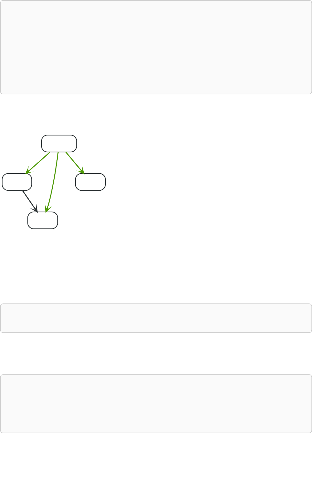
MERGE (p:Person {name: 'Joe'})
RETURN p
MATCH (a:Person {name: 'Joe'})
MERGE (b:Person {name: 'Jill'})
MERGE (a)-[r:LIKES]->(b)
MERGE (b)-[r1:EATS]->(f:Food {name: 'Margarita Pizza'})
RETURN a
MATCH (a:Person {name: 'Joe'})
MERGE (b:Person {name: 'Jill'})
MERGE (a)-[r:LIKES]->(b)
MERGE (b)-[r1:EATS]->(f:Food {name: 'Banana'})
RETURN a
We note that all these queries can also be combined into a single, larger query.
The CREATE UNIQUE examples below use the following graph:
name = 'A'
name = 'C'
KNOWS
name = 'B'
name = 'root'
X
X
X
3.18.2. Create unique nodes
Create node if missing
If the pattern described needs a node, and it can’t be matched, a new node will be created.
Query
MATCH (root { name: 'root' })
CREATE UNIQUE (root)-[:LOVES]-(someone)
RETURN someone
The root node doesn’t have any LOVES relationships, and so a node is created, and also a relationship
to that node.
Result
+------------+
| someone |
+------------+
| Node[20]{} |
+------------+
1 row
Nodes created: 1
Relationships created: 1
Create nodes with values
The pattern described can also contain values on the node. These are given using the following
144

syntax: prop: <expression>.
Query
MATCH (root { name: 'root' })
CREATE UNIQUE (root)-[:X]-(leaf { name: 'D' })
RETURN leaf
No node connected with the root node has the name D, and so a new node is created to match the
pattern.
Result
+--------------------+
| leaf |
+--------------------+
| Node[20]{name:"D"} |
+--------------------+
1 row
Nodes created: 1
Relationships created: 1
Properties set: 1
Create labeled node if missing
If the pattern described needs a labeled node and there is none with the given labels, Cypher will
create a new one.
Query
MATCH (a { name: 'A' })
CREATE UNIQUE (a)-[:KNOWS]-(c:blue)
RETURN c
The 'A' node is connected in a KNOWS relationship to the 'c' node, but since 'C' doesn’t have the blue
label, a new node labeled as blue is created along with a KNOWS relationship from 'A' to it.
Result
+------------+
| c |
+------------+
| Node[20]{} |
+------------+
1 row
Nodes created: 1
Relationships created: 1
Labels added: 1
3.18.3. Create unique relationships
Create relationship if it is missing
CREATE UNIQUE is used to describe the pattern that should be found or created.
Query
MATCH (lft { name: 'A' }),(rgt)
WHERE rgt.name IN ['B', 'C']
CREATE UNIQUE (lft)-[r:KNOWS]->(rgt)
RETURN r
145

The left node is matched against the two right nodes. One relationship already exists and can be
matched, and the other relationship is created before it is returned.
Result
+--------------+
| r |
+--------------+
| :KNOWS[20]{} |
| :KNOWS[3]{} |
+--------------+
2 rows
Relationships created: 1
Create relationship with values
Relationships to be created can also be matched on values.
Query
MATCH (root { name: 'root' })
CREATE UNIQUE (root)-[r:X { since: 'forever' }]-()
RETURN r
In this example, we want the relationship to have a value, and since no such relationship can be
found, a new node and relationship are created. Note that since we are not interested in the created
node, we don’t name it.
Result
+-------------------------+
| r |
+-------------------------+
| :X[20]{since:"forever"} |
+-------------------------+
1 row
Nodes created: 1
Relationships created: 1
Properties set: 1
3.18.4. Describe complex pattern
The pattern described by CREATE UNIQUE can be separated by commas, just like in MATCH and CREATE.
Query
MATCH (root { name: 'root' })
CREATE UNIQUE (root)-[:FOO]->(x),(root)-[:BAR]->(x)
RETURN x
This example pattern uses two paths, separated by a comma.
Result
+------------+
| x |
+------------+
| Node[20]{} |
+------------+
1 row
Nodes created: 1
Relationships created: 2
146
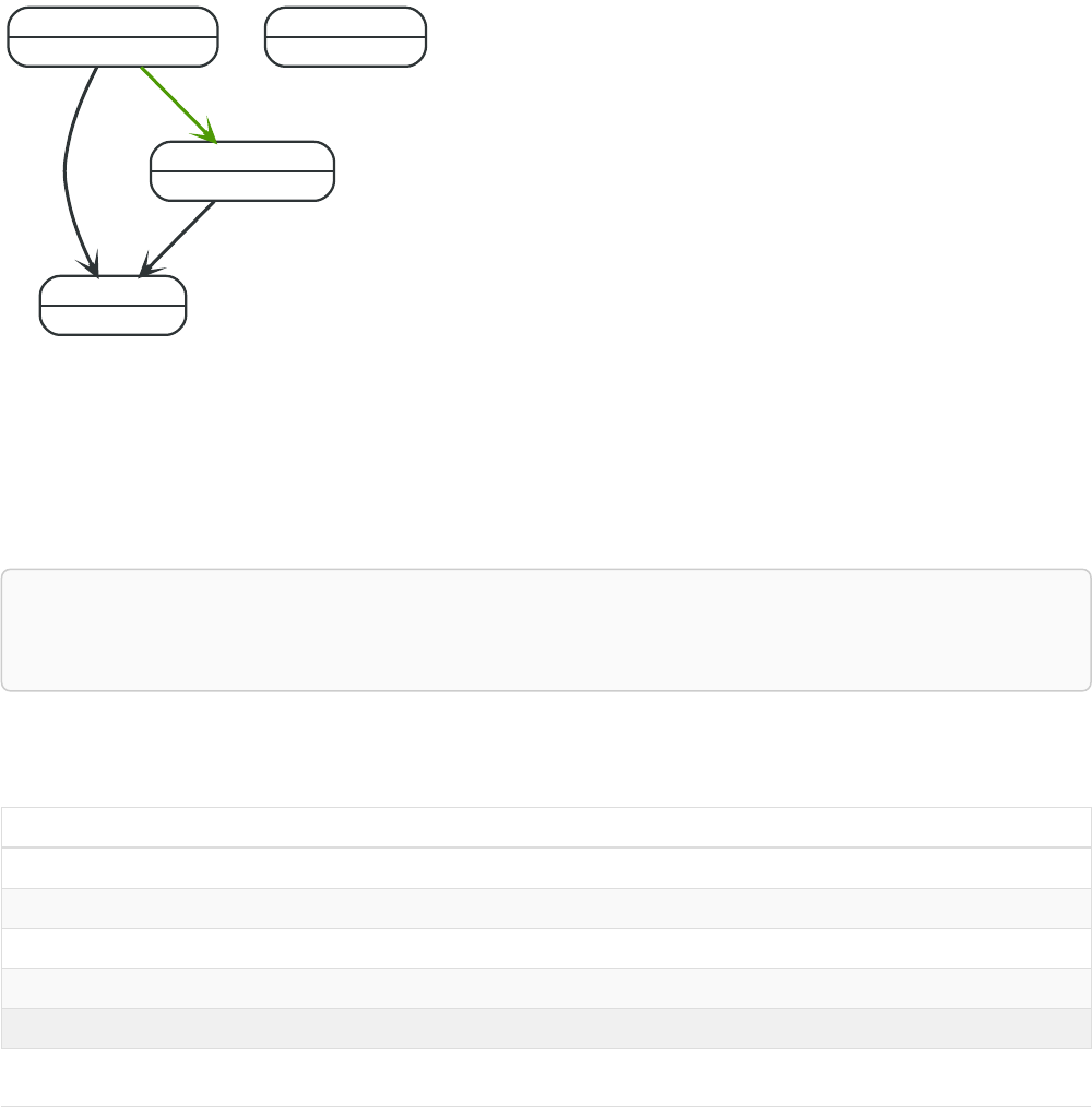
3.19. UNION
The UNION clause is used to combine the result of multiple queries.
•Introduction
•Combine two queries and retain duplicates
•Combine two queries and remove duplicates
3.19.1. Introduction
UNION combines the results of two or more queries into a single result set that includes all the rows
that belong to all queries in the union.
The number and the names of the columns must be identical in all queries combined by using UNION.
To keep all the result rows, use UNION ALL. Using just UNION will combine and remove duplicates from
the result set.
Actor
name = 'Anthony Hopkins'
Movie
title = 'Hitchcock'
ACTS_IN Actor
name = 'Helen Mirren'
KNOWS
ACTS_IN
Actor
name = 'Hitchcock'
Figure 21. Graph
3.19.2. Combine two queries and retain duplicates
Combining the results from two queries is done using UNION ALL.
Query
MATCH (n:Actor)
RETURN n.name AS name
UNION ALL MATCH (n:Movie)
RETURN n.title AS name
The combined result is returned, including duplicates.
Table 211. Result
name
"Anthony Hopkins"
"Helen Mirren"
"Hitchcock"
"Hitchcock"
4 rows
147

3.19.3. Combine two queries and remove duplicates
By not including ALL in the UNION, duplicates are removed from the combined result set
Query
MATCH (n:Actor)
RETURN n.name AS name
UNION
MATCH (n:Movie)
RETURN n.title AS name
The combined result is returned, without duplicates.
Table 212. Result
name
"Anthony Hopkins"
"Helen Mirren"
"Hitchcock"
3 rows
3.20. LOAD CSV
LOAD CSV is used to import data from CSV files.
•Introduction
•CSV file format
•Import data from a CSV file
•Import data from a CSV file containing headers
•Import data from a CSV file with a custom field delimiter
•Importing large amounts of data
•Setting the rate of periodic commits
•Import data containing escaped characters
3.20.1. Introduction
•The URL of the CSV file is specified by using FROM followed by an arbitrary expression evaluating to
the URL in question.
•It is required to specify a variable for the CSV data using AS.
•LOAD CSV supports resources compressed with gzip, Deflate, as well as ZIP archives.
•CSV files can be stored on the database server and are then accessible using a file:/// URL.
Alternatively, LOAD CSV also supports accessing CSV files via HTTPS, HTTP, and FTP.
•LOAD CSV will follow HTTP redirects but for security reasons it will not follow redirects that changes
the protocol, for example if the redirect is going from HTTPS to HTTP.
•LOAD CSV is often used in conjunction with the query hint PERIODIC COMMIT; more information on
this may be found in PERIODIC COMMIT query hint.
Configuration settings for file URLs
148

dbms.security.allow_csv_import_from_file_urls
This setting determines if Cypher will allow the use of file:/// URLs when loading data using LOAD
CSV. Such URLs identify files on the filesystem of the database server. Default is true. Setting
dbms.security.allow_csv_import_from_file_urls=false will completely disable access to the file
system for LOAD CSV.
dbms.directories.import
Sets the root directory for file:/// URLs used with the Cypher LOAD CSV clause. This must be set to
a single directory on the filesystem of the database server, and will make all requests to load from
file:/// URLs relative to the specified directory (similar to how a Unix chroot operates). The
default value is import. This is a security measure which prevents the database from accessing files
outside the standard import directory. Setting dbms.directories.import to be empty removes this
security measure and instead allows access to any file on the system. This is not recommended.
File URLs will be resolved relative to the dbms.directories.import directory. For example, a file URL will
typically look like file:///myfile.csv or file:///myproject/myfile.csv.
•If dbms.directories.import is set to the default value import, using the above URLs in LOAD CSV
would read from <NEO4J_HOME>/import/myfile.csv and <NEO4J_HOME>import/myproject/myfile.csv
respectively.
•If it is set to /data/csv, using the above URLs in LOAD CSV would read from /data/csv/myfile.csv and
/data/csv/myproject/myfile.csv respectively.
See the examples below for further details.
There is also a worked example, see getting-started.pdf.
3.20.2. CSV file format
The CSV file to use with LOAD CSV must have the following characteristics:
•the character encoding is UTF-8;
•the end line termination is system dependent, e.g., it is \n on unix or \r\n on windows;
•the default field terminator is ,;
•the field terminator character can be change by using the option FIELDTERMINATOR available in the
LOAD CSV command;
•quoted strings are allowed in the CSV file and the quotes are dropped when reading the data;
•the character for string quotation is double quote ";
•if dbms.import.csv.legacy_quote_escaping is set to the default value of true, \ is used as an escape
character;
•a double quote must be in a quoted string and escaped, either with the escape character or a
second double quote.
3.20.3. Import data from a CSV file
To import data from a CSV file into Neo4j, you can use LOAD CSV to get the data into your query. Then
you write it to your database using the normal updating clauses of Cypher.
artists.csv
1,ABBA,1992
2,Roxette,1986
3,Europe,1979
4,The Cardigans,1992
149

Query
LOAD CSV FROM 'https://neo4j.com/docs/cypher-manual/3.5/csv/artists.csv' AS line
CREATE (:Artist { name: line[1], year: toInteger(line[2])})
A new node with the Artist label is created for each row in the CSV file. In addition, two columns from
the CSV file are set as properties on the nodes.
Result
+-------------------+
| No data returned. |
+-------------------+
Nodes created: 4
Properties set: 8
Labels added: 4
3.20.4. Import data from a CSV file containing headers
When your CSV file has headers, you can view each row in the file as a map instead of as an array of
strings.
artists-with-headers.csv
Id,Name,Year
1,ABBA,1992
2,Roxette,1986
3,Europe,1979
4,The Cardigans,1992
Query
LOAD CSV WITH HEADERS FROM 'https://neo4j.com/docs/cypher-manual/3.5/csv/artists-with-headers.csv' AS line
CREATE (:Artist { name: line.Name, year: toInteger(line.Year)})
This time, the file starts with a single row containing column names. Indicate this using WITH HEADERS
and you can access specific fields by their corresponding column name.
Result
+-------------------+
| No data returned. |
+-------------------+
Nodes created: 4
Properties set: 8
Labels added: 4
3.20.5. Import data from a CSV file with a custom field delimiter
Sometimes, your CSV file has other field delimiters than commas. You can specify which delimiter
your file uses, using FIELDTERMINATOR. Hexadecimal representation of the unicode character encoding
can be used if prepended by \u. The encoding must be written with four digits. For example, \u002C is
equivalent to ;.
artists-fieldterminator.csv
1;ABBA;1992
2;Roxette;1986
3;Europe;1979
4;The Cardigans;1992
150

Query
LOAD CSV FROM 'https://neo4j.com/docs/cypher-manual/3.5/csv/artists-fieldterminator.csv' AS line
FIELDTERMINATOR ';'
CREATE (:Artist { name: line[1], year: toInteger(line[2])})
As values in this file are separated by a semicolon, a custom FIELDTERMINATOR is specified in the LOAD
CSV clause.
Result
+-------------------+
| No data returned. |
+-------------------+
Nodes created: 4
Properties set: 8
Labels added: 4
3.20.6. Importing large amounts of data
If the CSV file contains a significant number of rows (approaching hundreds of thousands or millions),
USING PERIODIC COMMIT can be used to instruct Neo4j to perform a commit after a number of rows.
This reduces the memory overhead of the transaction state. By default, the commit will happen every
1000 rows. For more information, see PERIODIC COMMIT query hint.
Query
USING PERIODIC COMMIT
LOAD CSV FROM 'https://neo4j.com/docs/cypher-manual/3.5/csv/artists.csv' AS line
CREATE (:Artist { name: line[1], year: toInteger(line[2])})
Result
+-------------------+
| No data returned. |
+-------------------+
Nodes created: 4
Properties set: 8
Labels added: 4
3.20.7. Setting the rate of periodic commits
You can set the number of rows as in the example, where it is set to 500 rows.
Query
USING PERIODIC COMMIT 500
LOAD CSV FROM 'https://neo4j.com/docs/cypher-manual/3.5/csv/artists.csv' AS line
CREATE (:Artist { name: line[1], year: toInteger(line[2])})
Result
+-------------------+
| No data returned. |
+-------------------+
Nodes created: 4
Properties set: 8
Labels added: 4
151

3.20.8. Import data containing escaped characters
In this example, we both have additional quotes around the values, as well as escaped quotes inside
one value.
artists-with-escaped-char.csv
"1","The ""Symbol""","1992"
Query
LOAD CSV FROM 'https://neo4j.com/docs/cypher-manual/3.5/csv/artists-with-escaped-char.csv' AS line
CREATE (a:Artist { name: line[1], year: toInteger(line[2])})
RETURN a.name AS name, a.year AS year, size(a.name) AS size
Note that strings are wrapped in quotes in the output here. You can see that when comparing to the
length of the string in this case!
Result
+------------------------------+
| name | year | size |
+------------------------------+
| "The "Symbol"" | 1992 | 12 |
+------------------------------+
1 row
Nodes created: 1
Properties set: 2
Labels added: 1
152

Chapter 4. Functions
This section contains information on all functions in the Cypher query language.
•Predicate functions [Summary|Detail]
•Scalar functions [Summary|Detail]
•Aggregating functions [Summary|Detail]
•List functions [Summary|Detail]
•Mathematical functions - numeric [Summary|Detail]
•Mathematical functions - logarithmic [Summary|Detail]
•Mathematical functions - trigonometric [Summary|Detail]
•String functions [Summary|Detail]
•Temporal functions - instant types [Summary|Detail]
•Temporal functions - duration [Summary|Detail]
•Spatial functions [Summary|Detail]
•User-defined functions
Related information may be found in Operators.
Please note
•Functions in Cypher return null if an input parameter is null.
•Functions taking a string as input all operate on Unicode characters rather than on a standard
char[]. For example, size(s), where s is a character in the Chinese alphabet, will return 1.
Predicate functions
These functions return either true or false for the given arguments.
Function Description
all() Tests whether the predicate holds for all elements in a list.
any() Tests whether the predicate holds for at least one element
in a list.
exists() Returns true if a match for the pattern exists in the graph,
or if the specified property exists in the node, relationship
or map.
none() Returns true if the predicate holds for no element in a list.
single() Returns true if the predicate holds for exactly one of the
elements in a list.
Scalar functions
These functions return a single value.
Function Description
coalesce() Returns the first non-null value in a list of expressions.
endNode() Returns the end node of a relationship.
head() Returns the first element in a list.
153

Function Description
id() Returns the id of a relationship or node.
last() Returns the last element in a list.
length() Returns the length of a path.
properties() Returns a map containing all the properties of a node or
relationship.
randomUUID() Returns a string value corresponding to a randomly-
generated UUID.
size() Returns the number of items in a list.
size() applied to pattern expression Returns the number of sub-graphs matching the pattern
expression.
size() applied to string Returns the number of Unicode characters in a string.
startNode() Returns the start node of a relationship.
timestamp() Returns the difference, measured in milliseconds, between
the current time and midnight, January 1, 1970 UTC.
toBoolean() Converts a string value to a boolean value.
toFloat() Converts an integer or string value to a floating point
number.
toInteger() Converts a floating point or string value to an integer
value.
type() Returns the string representation of the relationship type.
Aggregating functions
These functions take multiple values as arguments, and calculate and return an aggregated value
from them.
Function Description
avg() - Numeric values Returns the average of a set of numeric values.
avg() - Durations Returns the average of a set of Durations.
collect() Returns a list containing the values returned by an
expression.
count() Returns the number of values or rows.
max() Returns the maximum value in a set of values.
min() Returns the minimum value in a set of values.
percentileCont() Returns the percentile of a value over a group using linear
interpolation.
percentileDisc() Returns the nearest value to the given percentile over a
group using a rounding method.
stDev() Returns the standard deviation for the given value over a
group for a sample of a population.
stDevP() Returns the standard deviation for the given value over a
group for an entire population.
sum() - Numeric values Returns the sum of a set of numeric values.
sum() - Durations Returns the sum of a set of Durations.
List functions
These functions return lists of other values. Further details and examples of lists may be found in
154

Lists.
Function Description
extract() Returns a list lresult containing the values resulting from an
expression which has been applied to each element in a
list list.
filter() Returns a list lresult containing all the elements from a list
list that comply with a predicate.
keys() Returns a list containing the string representations for all
the property names of a node, relationship, or map.
labels() Returns a list containing the string representations for all
the labels of a node.
nodes() Returns a list containing all the nodes in a path.
range() Returns a list comprising all integer values within a
specified range.
reduce() Runs an expression against individual elements of a list,
storing the result of the expression in an accumulator.
relationships() Returns a list containing all the relationships in a path.
reverse() Returns a list in which the order of all elements in the
original list have been reversed.
tail() Returns all but the first element in a list.
Mathematical functions - numeric
These functions all operate on numerical expressions only, and will return an error if used on any
other values.
Function Description
abs() Returns the absolute value of a number.
ceil() Returns the smallest floating point number that is greater
than or equal to a number and equal to a mathematical
integer.
floor() Returns the largest floating point number that is less than
or equal to a number and equal to a mathematical integer.
rand() Returns a random floating point number in the range from
0 (inclusive) to 1 (exclusive); i.e. [0,1).
round() Returns the value of a number rounded to the nearest
integer.
sign() Returns the signum of a number: 0 if the number is 0, -1
for any negative number, and 1 for any positive number.
Mathematical functions - logarithmic
These functions all operate on numerical expressions only, and will return an error if used on any
other values.
Function Description
e() Returns the base of the natural logarithm, e.
exp() Returns e^n, where e is the base of the natural logarithm,
and n is the value of the argument expression.
log() Returns the natural logarithm of a number.
log10() Returns the common logarithm (base 10) of a number.
155

Function Description
sqrt() Returns the square root of a number.
Mathematical functions - trigonometric
These functions all operate on numerical expressions only, and will return an error if used on any
other values.
All trigonometric functions operate on radians, unless otherwise specified.
Function Description
acos() Returns the arccosine of a number in radians.
asin() Returns the arcsine of a number in radians.
atan() Returns the arctangent of a number in radians.
atan2() Returns the arctangent2 of a set of coordinates in radians.
cos() Returns the cosine of a number.
cot() Returns the cotangent of a number.
degrees() Converts radians to degrees.
haversin() Returns half the versine of a number.
pi() Returns the mathematical constant pi.
radians() Converts degrees to radians.
sin() Returns the sine of a number.
tan() Returns the tangent of a number.
String functions
These functions are used to manipulate strings or to create a string representation of another value.
Function Description
left() Returns a string containing the specified number of
leftmost characters of the original string.
lTrim() Returns the original string with leading whitespace
removed.
replace() Returns a string in which all occurrences of a specified
string in the original string have been replaced by another
(specified) string.
reverse() Returns a string in which the order of all characters in the
original string have been reversed.
right() Returns a string containing the specified number of
rightmost characters of the original string.
rTrim() Returns the original string with trailing whitespace
removed.
split() Returns a list of strings resulting from the splitting of the
original string around matches of the given delimiter.
substring() Returns a substring of the original string, beginning with a
0-based index start and length.
toLower() Returns the original string in lowercase.
toString() Converts an integer, float, boolean or temporal type (i.e.
Date, Time, LocalTime, DateTime, LocalDateTime or
Duration) value to a string.
156

Function Description
toUpper() Returns the original string in uppercase.
trim() Returns the original string with leading and trailing
whitespace removed.
Temporal functions - instant types
Values of the temporal types — Date, Time, LocalTime, DateTime, and LocalDateTime — can be created
manipulated using the following functions:
Function Description
date() Returns the current Date.
date.transaction() Returns the current Date using the transaction clock.
date.statement() Returns the current Date using the statement clock.
date.realtime() Returns the current Date using the realtime clock.
date({year [, month, day]}) Returns a calendar (Year-Month-Day) Date.
date({year [, week, dayOfWeek]}) Returns a week (Year-Week-Day) Date.
date({year [, quarter, dayOfQuarter]}) Returns a quarter (Year-Quarter-Day) Date.
date({year [, ordinalDay]}) Returns an ordinal (Year-Day) Date.
date(string) Returns a Date by parsing a string.
date({map}) Returns a Date from a map of another temporal value’s
components.
date.truncate() Returns a Date obtained by truncating a value at a specific
component boundary. Truncation summary.
datetime() Returns the current DateTime.
datetime.transaction() Returns the current DateTime using the transaction clock.
datetime.statement() Returns the current DateTime using the statement clock.
datetime.realtime() Returns the current DateTime using the realtime clock.
datetime({year [, month, day, …]}) Returns a calendar (Year-Month-Day) DateTime.
datetime({year [, week, dayOfWeek, …]}) Returns a week (Year-Week-Day) DateTime.
datetime({year [, quarter, dayOfQuarter, …]}) Returns a quarter (Year-Quarter-Day) DateTime.
datetime({year [, ordinalDay, …]}) Returns an ordinal (Year-Day) DateTime.
datetime(string) Returns a DateTime by parsing a string.
datetime({map}) Returns a DateTime from a map of another temporal
value’s components.
datetime({epochSeconds}) Returns a DateTime from a timestamp.
datetime.truncate() Returns a DateTime obtained by truncating a value at a
specific component boundary. Truncation summary.
localdatetime() Returns the current LocalDateTime.
localdatetime.transaction() Returns the current LocalDateTime using the transaction
clock.
localdatetime.statement() Returns the current LocalDateTime using the statement
clock.
localdatetime.realtime() Returns the current LocalDateTime using the realtime
clock.
localdatetime({year [, month, day, …]}) Returns a calendar (Year-Month-Day) LocalDateTime.
157

Function Description
localdatetime({year [, week, dayOfWeek, …]}) Returns a week (Year-Week-Day) LocalDateTime.
localdatetime({year [, quarter, dayOfQuarter, …]}) Returns a quarter (Year-Quarter-Day) DateTime.
localdatetime({year [, ordinalDay, …]}) Returns an ordinal (Year-Day) LocalDateTime.
localdatetime(string) Returns a LocalDateTime by parsing a string.
localdatetime({map}) Returns a LocalDateTime from a map of another temporal
value’s components.
localdatetime.truncate() Returns a LocalDateTime obtained by truncating a value at
a specific component boundary. Truncation summary.
localtime() Returns the current LocalTime.
localtime.transaction() Returns the current LocalTime using the transaction clock.
localtime.statement() Returns the current LocalTime using the statement clock.
localtime.realtime() Returns the current LocalTime using the realtime clock.
localtime({hour [, minute, second, …]}) Returns a LocalTime with the specified component values.
localtime(string) Returns a LocalTime by parsing a string.
localtime({time [, hour, …]}) Returns a LocalTime from a map of another temporal
value’s components.
localtime.truncate() Returns a LocalTime obtained by truncating a value at a
specific component boundary. Truncation summary.
time() Returns the current Time.
time.transaction() Returns the current Time using the transaction clock.
time.statement() Returns the current Time using the statement clock.
time.realtime() Returns the current Time using the realtime clock.
time({hour [, minute, …]}) Returns a Time with the specified component values.
time(string) Returns a Time by parsing a string.
time({time [, hour, …, timezone]}) Returns a Time from a map of another temporal value’s
components.
time.truncate() Returns a Time obtained by truncating a value at a specific
component boundary. Truncation summary.
Temporal functions - duration
Duration values of the temporal types can be created manipulated using the following functions:
Function Description
duration({map}) Returns a Duration from a map of its components.
duration(string) Returns a Duration by parsing a string.
duration.between() Returns a Duration equal to the difference between two
given instants.
duration.inMonths() Returns a Duration equal to the difference in whole
months, quarters or years between two given instants.
duration.inDays() Returns a Duration equal to the difference in whole days or
weeks between two given instants.
duration.inSeconds() Returns a Duration equal to the difference in seconds and
fractions of seconds, or minutes or hours, between two
given instants.
Spatial functions
158
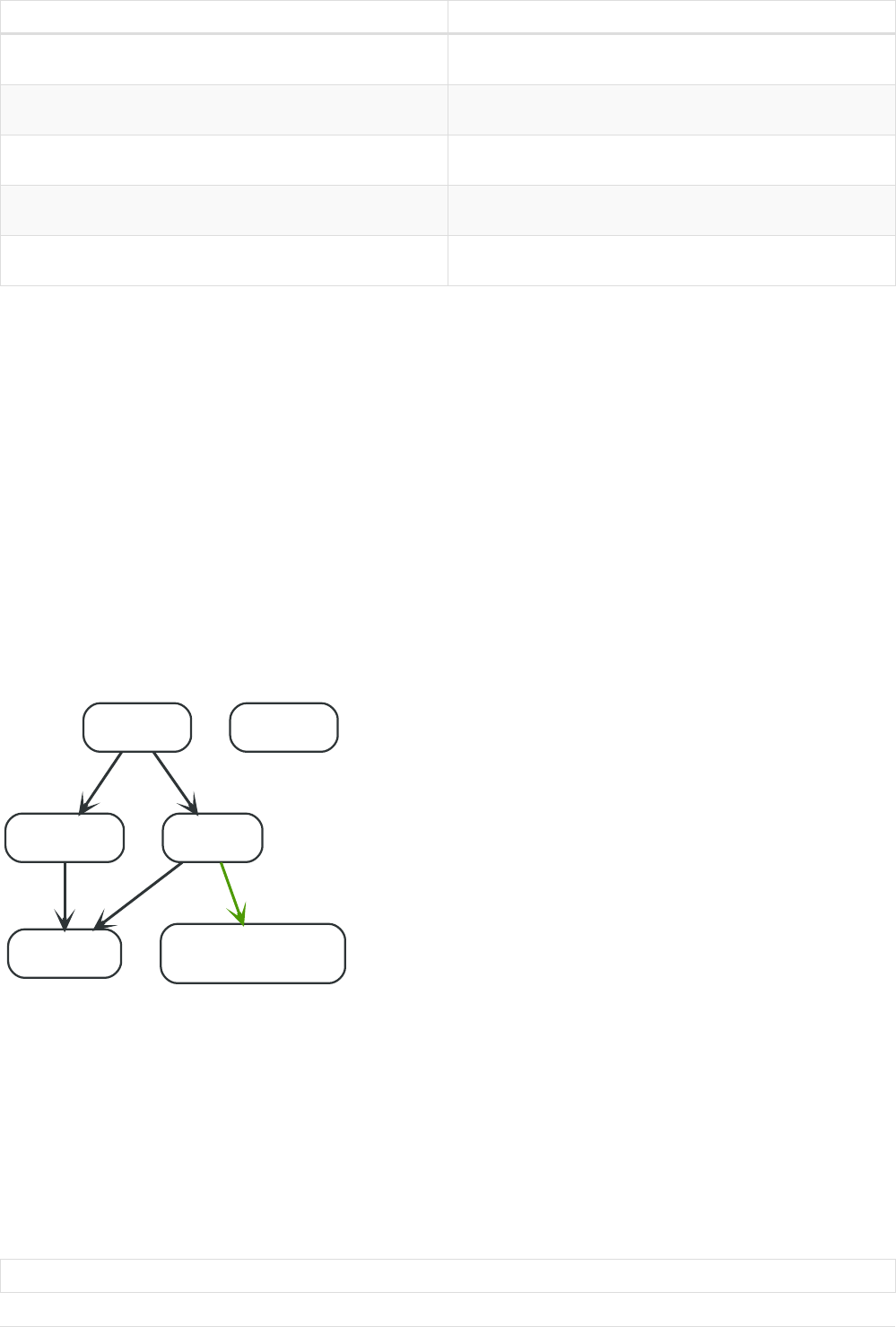
These functions are used to specify 2D or 3D points in a geographic or cartesian Coordinate Reference
System and to calculate the geodesic distance between two points.
Function Description
distance() Returns a floating point number representing the geodesic
distance between any two points in the same CRS.
point() - Cartesian 2D Returns a 2D point object, given two coordinate values in
the Cartesian coordinate system.
point() - Cartesian 3D Returns a 3D point object, given three coordinate values in
the Cartesian coordinate system.
point() - WGS 84 2D Returns a 2D point object, given two coordinate values in
the WGS 84 geographic coordinate system.
point() - WGS 84 3D Returns a 3D point object, given three coordinate values in
the WGS 84 geographic coordinate system.
4.1. Predicate functions
Predicates are boolean functions that return true or false for a given set of non-null input.
They are most commonly used to filter out subgraphs in the WHERE part of a query.
Functions:
•all()
•any()
•exists()
•none()
•single()
name = 'Alice'
eyes = 'brown'
age = 38
name = 'Charlie'
eyes = 'green'
age = 53
KNOWS
name = 'Bob'
eyes = 'blue'
age = 25
KNOWS
name = 'Daniel'
eyes = 'brown'
age = 54
KNOWS
array = ['one', 'two', 'three']
name = 'Eskil'
eyes = 'blue'
age = 41
MARRIEDKNOWS
eyes = 'brown'
age = 61
Figure 22. Graph
4.1.1. all()
all() returns true if the predicate holds for all elements in the given list. null is returned if the list is
null or all of its elements are null.
Syntax: all(variable IN list WHERE predicate)
Returns:
A Boolean.
159

Arguments:
Name Description
list An expression that returns a list.
variable This is the variable that can be used from within the
predicate.
predicate A predicate that is tested against all items in the list.
Query
MATCH p =(a)-[*1..3]->(b)
WHERE a.name = 'Alice' AND b.name = 'Daniel' AND ALL (x IN nodes(p) WHERE x.age > 30)
RETURN p
All nodes in the returned paths will have an age property of at least '30'.
Table 213. Result
p
(0)-[KNOWS,1]->(2)-[KNOWS,3]->(3)
1 row
4.1.2. any()
any() returns true if the predicate holds for at least one element in the given list. null is returned if
the list is null or all of its elements are null.
Syntax: any(variable IN list WHERE predicate)
Returns:
A Boolean.
Arguments:
Name Description
list An expression that returns a list.
variable This is the variable that can be used from within the
predicate.
predicate A predicate that is tested against all items in the list.
Query
MATCH (a)
WHERE a.name = 'Eskil' AND ANY (x IN a.array WHERE x = 'one')
RETURN a.name, a.array
All nodes in the returned paths have at least one 'one' value set in the array property named array.
Table 214. Result
a.name a.array
"Eskil" ["one","two","three"]
1 row
160

4.1.3. exists()
exists() returns true if a match for the given pattern exists in the graph, or if the specified property
exists in the node, relationship or map. null is returned if the input argument is null.
Syntax: exists(pattern-or-property)
Returns:
A Boolean.
Arguments:
Name Description
pattern-or-property A pattern or a property (in the form 'variable.prop').
Query
MATCH (n)
WHERE exists(n.name)
RETURN n.name AS name, exists((n)-[:MARRIED]->()) AS is_married
The names of all nodes with the name property are returned, along with a boolean true / false
indicating if they are married.
Table 215. Result
name is_married
"Alice" false
"Bob" true
"Charlie" false
"Daniel" false
"Eskil" false
5 rows
Query
MATCH (a),(b)
WHERE exists(a.name) AND NOT exists(b.name)
OPTIONAL MATCH (c:DoesNotExist)
RETURN a.name AS a_name, b.name AS b_name, exists(b.name) AS b_has_name, c.name AS c_name, exists(c.name)
AS c_has_name
ORDER BY a_name, b_name, c_name
LIMIT 1
Three nodes are returned: one with a name property, one without a name property, and one that
does not exist (e.g., is null). This query exemplifies the behavior of exists() when operating on null
nodes.
Table 216. Result
a_name b_name b_has_name c_name c_has_name
"Alice" <null> false <null> <null>
1 row
161

4.1.4. none()
none() returns true if the predicate holds for no element in the given list. null is returned if the list is
null or all of its elements are null.
Syntax: none(variable IN list WHERE predicate)
Returns:
A Boolean.
Arguments:
Name Description
list An expression that returns a list.
variable This is the variable that can be used from within the
predicate.
predicate A predicate that is tested against all items in the list.
Query
MATCH p =(n)-[*1..3]->(b)
WHERE n.name = 'Alice' AND NONE (x IN nodes(p) WHERE x.age = 25)
RETURN p
No node in the returned paths has an age property set to '25'.
Table 217. Result
p
(0)-[KNOWS,1]->(2)
(0)-[KNOWS,1]->(2)-[KNOWS,3]->(3)
2 rows
4.1.5. single()
single() returns true if the predicate holds for exactly one of the elements in the given list. null is
returned if the list is null or all of its elements are null.
Syntax: single(variable IN list WHERE predicate)
Returns:
A Boolean.
Arguments:
Name Description
list An expression that returns a list.
variable This is the variable that can be used from within the
predicate.
predicate A predicate that is tested against all items in the list.
162

Query
MATCH p =(n)-->(b)
WHERE n.name = 'Alice' AND SINGLE (var IN nodes(p) WHERE var.eyes = 'blue')
RETURN p
Exactly one node in every returned path has the eyes property set to 'blue'.
Table 218. Result
p
(0)-[KNOWS,0]->(1)
1 row
4.2. Scalar functions
Scalar functions return a single value.
The length() and size() functions are quite similar, and so it is important to take
note of the difference. Owing to backwards compatibility, length() currently
works on four types: strings, paths, lists and pattern expressions. However, it is
recommended to use length() only for paths, and the size() function for strings,
lists and pattern expressions. length() on those types may be deprecated in
future.
The timestamp() function returns the equivalent value of datetime().epochMillis.
The function toInt() has been superseded by toInteger(), and will be removed in a
future release.
Functions:
•coalesce()
•endNode()
•head()
•id()
•last()
•length()
•properties()
•randomUUID()
•size()
•Size of pattern expression
•Size of string
•startNode()
•timestamp()
•toBoolean()
•toFloat()
163
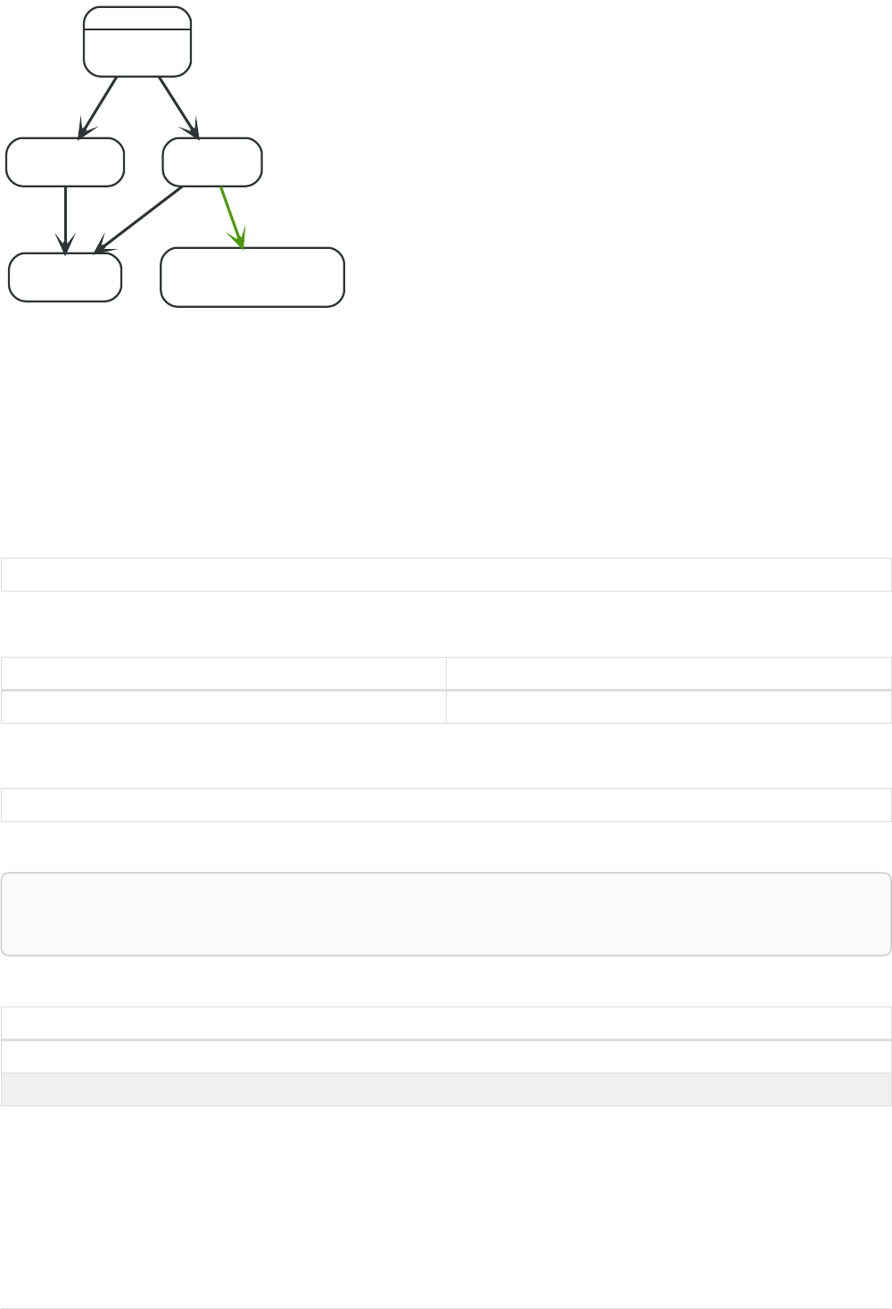
•toInteger()
•type()
Developer
name = 'Alice'
eyes = 'brown'
age = 38
name = 'Charlie'
eyes = 'green'
age = 53
KNOWS
name = 'Bob'
eyes = 'blue'
age = 25
KNOWS
name = 'Daniel'
eyes = 'brown'
age = 54
KNOWS
array = ['one', 'two', 'three']
name = 'Eskil'
eyes = 'blue'
age = 41
MARRIEDKNOWS
Figure 23. Graph
4.2.1. coalesce()
coalesce() returns the first non-null value in the given list of expressions.
Syntax: coalesce(expression [, expression]*)
Returns:
The type of the value returned will be that of the first non-null expression.
Arguments:
Name Description
expression An expression which may return null.
Considerations:
null will be returned if all the arguments are null.
Query
MATCH (a)
WHERE a.name = 'Alice'
RETURN coalesce(a.hairColor, a.eyes)
Table 219. Result
coalesce(a.hairColor, a.eyes)
"brown"
1 row
4.2.2. endNode()
endNode() returns the end node of a relationship.
Syntax: endNode(relationship)
164

Returns:
A Node.
Arguments:
Name Description
relationship An expression that returns a relationship.
Considerations:
endNode(null) returns null.
Query
MATCH (x:Developer)-[r]-()
RETURN endNode(r)
Table 220. Result
endNode(r)
Node[2]{name:"Charlie",eyes:"green",age:53}
Node[1]{name:"Bob",eyes:"blue",age:25}
2 rows
4.2.3. head()
head() returns the first element in a list.
Syntax: head(list)
Returns:
The type of the value returned will be that of the first element of list.
Arguments:
Name Description
list An expression that returns a list.
Considerations:
head(null) returns null.
If the first element in list is null, head(list) will return null.
Query
MATCH (a)
WHERE a.name = 'Eskil'
RETURN a.array, head(a.array)
The first element in the list is returned.
Table 221. Result
165

a.array head(a.array)
["one","two","three"] "one"
1 row
4.2.4. id()
id() returns the id of a relationship or node.
Syntax: id(expression)
Returns:
An Integer.
Arguments:
Name Description
expression An expression that returns a node or a relationship.
Considerations:
id(null) returns null.
Query
MATCH (a)
RETURN id(a)
The node id for each of the nodes is returned.
Table 222. Result
id(a)
0
1
2
3
4
5 rows
4.2.5. last()
last() returns the last element in a list.
Syntax: last(expression)
Returns:
The type of the value returned will be that of the last element of list.
Arguments:
166

Name Description
list An expression that returns a list.
Considerations:
last(null) returns null.
If the last element in list is null, last(list) will return null.
Query
MATCH (a)
WHERE a.name = 'Eskil'
RETURN a.array, last(a.array)
The last element in the list is returned.
Table 223. Result
a.array last(a.array)
["one","two","three"] "three"
1 row
4.2.6. length()
length() returns the length of a path.
Syntax: length(path)
Returns:
An Integer.
Arguments:
Name Description
path An expression that returns a path.
Considerations:
length(null) returns null.
Query
MATCH p =(a)-->(b)-->(c)
WHERE a.name = 'Alice'
RETURN length(p)
The length of the path p is returned.
Table 224. Result
length(p)
2
2
167

length(p)
2
3 rows
4.2.7. properties()
properties() returns a map containing all the properties of a node or relationship. If the argument is
already a map, it is returned unchanged.
Syntax: properties(expression)
Returns:
A Map.
Arguments:
Name Description
expression An expression that returns a node, a relationship, or a
map.
Considerations:
properties(null) returns null.
Query
CREATE (p:Person { name: 'Stefan', city: 'Berlin' })
RETURN properties(p)
Table 225. Result
properties(p)
{city -> "Berlin", name -> "Stefan"}
1 row
Nodes created: 1
Properties set: 2
Labels added: 1
4.2.8. randomUUID()
randomUUID() returns a randomly-generated Universally Unique Identifier (UUID), also known as a
Globally Unique Identifier (GUID). This is a 128-bit value with strong guarantees of uniqueness.
Syntax: randomUUID()
Returns:
A String.
Query
RETURN randomUUID() AS uuid
Table 226. Result
168

uuid
"b1e31cc3-4245-4970-ac0d-00dde724fc61"
1 row
A randomly-generated UUID is returned.
4.2.9. size()
size() returns the number of elements in a list.
Syntax: size(list)
Returns:
An Integer.
Arguments:
Name Description
list An expression that returns a list.
Considerations:
size(null) returns null.
Query
RETURN size(['Alice', 'Bob'])
Table 227. Result
size(['Alice', 'Bob'])
2
1 row
The number of elements in the list is returned.
4.2.10. size() applied to pattern expression
This is the same size() method as described above, but instead of passing in a list directly, a pattern
expression can be provided that can be used in a match query to provide a new set of results. These
results are a list of paths. The size of the result is calculated, not the length of the expression itself.
Syntax: size(pattern expression)
Arguments:
Name Description
pattern expression A pattern expression that returns a list.
169

Query
MATCH (a)
WHERE a.name = 'Alice'
RETURN size((a)-->()-->()) AS fof
Table 228. Result
fof
3
1 row
The number of sub-graphs matching the pattern expression is returned.
4.2.11. size() applied to string
size() returns the number of Unicode characters in a string.
Syntax: size(string)
Returns:
An Integer.
Arguments:
Name Description
string An expression that returns a string value.
Considerations:
size(null) returns null.
Query
MATCH (a)
WHERE size(a.name)> 6
RETURN size(a.name)
Table 229. Result
size(a.name)
7
1 row
The number of characters in the string 'Charlie' is returned.
4.2.12. startNode()
startNode() returns the start node of a relationship.
Syntax: startNode(relationship)
Returns:
170

A Node.
Arguments:
Name Description
relationship An expression that returns a relationship.
Considerations:
startNode(null) returns null.
Query
MATCH (x:Developer)-[r]-()
RETURN startNode(r)
Table 230. Result
startNode(r)
Node[0]{name:"Alice",eyes:"brown",age:38}
Node[0]{name:"Alice",eyes:"brown",age:38}
2 rows
4.2.13. timestamp()
timestamp() returns the difference, measured in milliseconds, between the current time and midnight,
January 1, 1970 UTC.
Syntax: timestamp()
Returns:
An Integer.
Considerations:
timestamp() will return the same value during one entire query, even for long-running queries.
Query
RETURN timestamp()
The time in milliseconds is returned.
Table 231. Result
timestamp()
1544445444949
1 row
4.2.14. toBoolean()
toBoolean() converts a string value to a boolean value.
171

Syntax: toBoolean(expression)
Returns:
A Boolean.
Arguments:
Name Description
expression An expression that returns a boolean or string value.
Considerations:
toBoolean(null) returns null.
If expression is a boolean value, it will be returned unchanged.
If the parsing fails, null will be returned.
Query
RETURN toBoolean('TRUE'), toBoolean('not a boolean')
Table 232. Result
toBoolean('TRUE') toBoolean('not a boolean')
true <null>
1 row
4.2.15. toFloat()
toFloat() converts an integer or string value to a floating point number.
Syntax: toFloat(expression)
Returns:
A Float.
Arguments:
Name Description
expression An expression that returns a numeric or string value.
Considerations:
toFloat(null) returns null.
If expression is a floating point number, it will be returned unchanged.
If the parsing fails, null will be returned.
Query
RETURN toFloat('11.5'), toFloat('not a number')
172

Table 233. Result
toFloat('11.5') toFloat('not a number')
11.5 <null>
1 row
4.2.16. toInteger()
toInteger() converts a floating point or string value to an integer value.
Syntax: toInteger(expression)
Returns:
An Integer.
Arguments:
Name Description
expression An expression that returns a numeric or string value.
Considerations:
toInteger(null) returns null.
If expression is an integer value, it will be returned unchanged.
If the parsing fails, null will be returned.
Query
RETURN toInteger('42'), toInteger('not a number')
Table 234. Result
toInteger('42') toInteger('not a number')
42 <null>
1 row
4.2.17. type()
type() returns the string representation of the relationship type.
Syntax: type(relationship)
Returns:
A String.
Arguments:
Name Description
relationship An expression that returns a relationship.
Considerations:
173

type(null) returns null.
Query
MATCH (n)-[r]->()
WHERE n.name = 'Alice'
RETURN type(r)
The relationship type of r is returned.
Table 235. Result
type(r)
"KNOWS"
"KNOWS"
2 rows
4.3. Aggregating functions
To calculate aggregated data, Cypher offers aggregation, analogous to SQL’s GROUP BY.
Aggregating functions take a set of values and calculate an aggregated value over them. Examples are
avg() that calculates the average of multiple numeric values, or min() that finds the smallest numeric
or string value in a set of values. When we say below that an aggregating function operates on a set of
values, we mean these to be the result of the application of the inner expression (such as n.age) to all
the records within the same aggregation group.
Aggregation can be computed over all the matching subgraphs, or it can be further divided by
introducing grouping keys. These are non-aggregate expressions, that are used to group the values
going into the aggregate functions.
Assume we have the following return statement:
RETURN n, count(*)
We have two return expressions: n, and count(). The first, n, is not an aggregate function, and
so it will be the grouping key. The latter, count() is an aggregate expression. The matching
subgraphs will be divided into different buckets, depending on the grouping key. The aggregate
function will then be run on these buckets, calculating an aggregate value per bucket.
To use aggregations to sort the result set, the aggregation must be included in the RETURN to be used in
the ORDER BY.
The DISTINCT operator works in conjunction with aggregation. It is used to make all values unique
before running them through an aggregate function. More information about DISTINCT may be found
here.
Functions:
•avg() - Numeric values
•avg() - Durations
•collect()
•count()
•max()
174

•min()
•percentileCont()
•percentileDisc()
•stDev()
•stDevP()
•sum() - Numeric values
•sum() - Durations
The following graph is used for the examples below:
Person
name = 'A'
age = 13
Person
name = 'B'
age = 33
eyes = 'blue'
KNOWS
Person
name = 'C'
age = 44
eyes = 'blue'
KNOWS
Person
name = 'D'
eyes = 'brown'
KNOWS
Person
name = 'D'
KNOWS KNOWS
Figure 24. Graph
4.3.1. avg() - Numeric values
avg() returns the average of a set of numeric values.
Syntax: avg(expression)
Returns:
Either an Integer or a Float, depending on the values returned by expression and whether or not the calculation
overflows.
Arguments:
Name Description
expression An expression returning a set of numeric values.
Considerations:
Any null values are excluded from the calculation.
avg(null) returns null.
Query
MATCH (n:Person)
RETURN avg(n.age)
The average of all the values in the property age is returned.
175

Table 236. Result
avg(n.age)
30.0
1 row
4.3.2. avg() - Durations
avg() returns the average of a set of Durations.
Syntax: avg(expression)
Returns:
A Duration.
Arguments:
Name Description
expression An expression returning a set of Durations.
Considerations:
Any null values are excluded from the calculation.
avg(null) returns null.
Query
UNWIND [duration('P2DT3H'), duration('PT1H45S')] AS dur
RETURN avg(dur)
The average of the two supplied Durations is returned.
Table 237. Result
avg(dur)
P1DT2H22.5S
1 row
4.3.3. collect()
collect() returns a list containing the values returned by an expression. Using this function
aggregates data by amalgamating multiple records or values into a single list.
Syntax: collect(expression)
Returns:
A list containing heterogeneous elements; the types of the elements are determined by the values returned by
expression.
Arguments:
176

Name Description
expression An expression returning a set of values.
Considerations:
Any null values are ignored and will not be added to the list.
collect(null) returns an empty list.
Query
MATCH (n:Person)
RETURN collect(n.age)
All the values are collected and returned in a single list.
Table 238. Result
collect(n.age)
[13,33,44]
1 row
4.3.4. count()
count() returns the number of values or rows, and appears in two variants:
•count(*) returns the number of matching rows, and
•count(expr) returns the number of non-null values returned by an expression.
Syntax: count(expression)
Returns:
An Integer.
Arguments:
Name Description
expression An expression.
Considerations:
count(*) includes rows returning null.
count(expr) ignores null values.
count(null) returns 0.
Using count(*) to return the number of nodes
count(*) can be used to return the number of nodes; for example, the number of nodes connected to
some node n.
177

Query
MATCH (n { name: 'A' })-->(x)
RETURN labels(n), n.age, count(*)
The labels and age property of the start node n and the number of nodes related to n are returned.
Table 239. Result
labels(n) n.age count(*)
["Person"] 13 3
1 row
Using count(*) to group and count relationship types
count(*) can be used to group relationship types and return the number.
Query
MATCH (n { name: 'A' })-[r]->()
RETURN type(r), count(*)
The relationship types and their group count are returned.
Table 240. Result
type(r) count(*)
"KNOWS" 3
1 row
Using count(expression) to return the number of values
Instead of simply returning the number of rows with count(*), it may be more useful to return the
actual number of values returned by an expression.
Query
MATCH (n { name: 'A' })-->(x)
RETURN count(x)
The number of nodes connected to the start node is returned.
Table 241. Result
count(x)
3
1 row
Counting non-null values
count(expression) can be used to return the number of non-null values returned by the expression.
178

Query
MATCH (n:Person)
RETURN count(n.age)
The number of :Person nodes having an age property is returned.
Table 242. Result
count(n.age)
3
1 row
Counting with and without duplicates
In this example we are trying to find all our friends of friends, and count them:
•The first aggregate function, count(DISTINCT friend_of_friend), will only count a friend_of_friend
once, as DISTINCT removes the duplicates.
•The second aggregate function, count(friend_of_friend), will consider the same friend_of_friend
multiple times.
Query
MATCH (me:Person)-->(friend:Person)-->(friend_of_friend:Person)
WHERE me.name = 'A'
RETURN count(DISTINCT friend_of_friend), count(friend_of_friend)
Both B and C know D and thus D will get counted twice when not using DISTINCT.
Table 243. Result
count(DISTINCT friend_of_friend) count(friend_of_friend)
1 2
1 row
4.3.5. max()
max() returns the maximum value in a set of values.
Syntax: max(expression)
Returns:
A property type, or a list, depending on the values returned by expression.
Arguments:
Name Description
expression An expression returning a set containing any combination
of property types and lists thereof.
Considerations:
Any null values are excluded from the calculation.
179

In a mixed set, any numeric value is always considered to be higher than any string value, and any string value is
always considered to be higher than any list.
Lists are compared in dictionary order, i.e. list elements are compared pairwise in ascending order from the start of the
list to the end.
max(null) returns null.
Query
UNWIND [1, 'a', NULL , 0.2, 'b', '1', '99'] AS val
RETURN max(val)
The highest of all the values in the mixed set — in this case, the numeric value 1 — is returned. Note
that the (string) value "99", which may appear at first glance to be the highest value in the list, is
considered to be a lower value than 1 as the latter is a string.
Table 244. Result
max(val)
1
1 row
Query
UNWIND [[1, 'a', 89],[1, 2]] AS val
RETURN max(val)
The highest of all the lists in the set — in this case, the list [1, 2] — is returned, as the number 2 is
considered to be a higher value than the string "a", even though the list [1, 'a', 89] contains more
elements.
Table 245. Result
max(val)
[1,2]
1 row
Query
MATCH (n:Person)
RETURN max(n.age)
The highest of all the values in the property age is returned.
Table 246. Result
max(n.age)
44
1 row
4.3.6. min()
min() returns the minimum value in a set of values.
Syntax: min(expression)
180

Returns:
A property type, or a list, depending on the values returned by expression.
Arguments:
Name Description
expression An expression returning a set containing any combination
of property types and lists thereof.
Considerations:
Any null values are excluded from the calculation.
In a mixed set, any string value is always considered to be lower than any numeric value, and any list is always
considered to be lower than any string.
Lists are compared in dictionary order, i.e. list elements are compared pairwise in ascending order from the start of the
list to the end.
min(null) returns null.
Query
UNWIND [1, 'a', NULL , 0.2, 'b', '1', '99'] AS val
RETURN min(val)
The lowest of all the values in the mixed set — in this case, the string value "1" — is returned. Note
that the (numeric) value 0.2, which may appear at first glance to be the lowest value in the list, is
considered to be a higher value than "1" as the latter is a string.
Table 247. Result
min(val)
"1"
1 row
Query
UNWIND ['d',[1, 2],['a', 'c', 23]] AS val
RETURN min(val)
The lowest of all the values in the set — in this case, the list ['a', 'c', 23] — is returned, as (i) the two
lists are considered to be lower values than the string "d", and (ii) the string "a" is considered to be a
lower value than the numerical value 1.
Table 248. Result
min(val)
["a","c",23]
1 row
Query
MATCH (n:Person)
RETURN min(n.age)
The lowest of all the values in the property age is returned.
181

Table 249. Result
min(n.age)
13
1 row
4.3.7. percentileCont()
percentileCont() returns the percentile of the given value over a group, with a percentile from 0.0 to
1.0. It uses a linear interpolation method, calculating a weighted average between two values if the
desired percentile lies between them. For nearest values using a rounding method, see
percentileDisc.
Syntax: percentileCont(expression, percentile)
Returns:
A Float.
Arguments:
Name Description
expression A numeric expression.
percentile A numeric value between 0.0 and 1.0
Considerations:
Any null values are excluded from the calculation.
percentileCont(null, percentile) returns null.
Query
MATCH (n:Person)
RETURN percentileCont(n.age, 0.4)
The 40th percentile of the values in the property age is returned, calculated with a weighted average.
In this case, 0.4 is the median, or 40th percentile.
Table 250. Result
percentileCont(n.age, 0.4)
29.0
1 row
4.3.8. percentileDisc()
percentileDisc() returns the percentile of the given value over a group, with a percentile from 0.0 to
1.0. It uses a rounding method and calculates the nearest value to the percentile. For interpolated
values, see percentileCont.
Syntax: percentileDisc(expression, percentile)
Returns:
182

Either an Integer or a Float, depending on the values returned by expression and whether or not the calculation
overflows.
Arguments:
Name Description
expression A numeric expression.
percentile A numeric value between 0.0 and 1.0
Considerations:
Any null values are excluded from the calculation.
percentileDisc(null, percentile) returns null.
Query
MATCH (n:Person)
RETURN percentileDisc(n.age, 0.5)
The 50th percentile of the values in the property age is returned.
Table 251. Result
percentileDisc(n.age, 0.5)
33
1 row
4.3.9. stDev()
stDev() returns the standard deviation for the given value over a group. It uses a standard two-pass
method, with N - 1 as the denominator, and should be used when taking a sample of the population
for an unbiased estimate. When the standard variation of the entire population is being calculated,
stdDevP should be used.
Syntax: stDev(expression)
Returns:
A Float.
Arguments:
Name Description
expression A numeric expression.
Considerations:
Any null values are excluded from the calculation.
stDev(null) returns 0.
183

Query
MATCH (n)
WHERE n.name IN ['A', 'B', 'C']
RETURN stDev(n.age)
The standard deviation of the values in the property age is returned.
Table 252. Result
stDev(n.age)
15.716233645501712
1 row
4.3.10. stDevP()
stDevP() returns the standard deviation for the given value over a group. It uses a standard two-pass
method, with N as the denominator, and should be used when calculating the standard deviation for
an entire population. When the standard variation of only a sample of the population is being
calculated, stDev should be used.
Syntax: stDevP(expression)
Returns:
A Float.
Arguments:
Name Description
expression A numeric expression.
Considerations:
Any null values are excluded from the calculation.
stDevP(null) returns 0.
Query
MATCH (n)
WHERE n.name IN ['A', 'B', 'C']
RETURN stDevP(n.age)
The population standard deviation of the values in the property age is returned.
Table 253. Result
stDevP(n.age)
12.832251036613439
1 row
4.3.11. sum() - Numeric values
sum() returns the sum of a set of numeric values.
184

Syntax: sum(expression)
Returns:
Either an Integer or a Float, depending on the values returned by expression.
Arguments:
Name Description
expression An expression returning a set of numeric values.
Considerations:
Any null values are excluded from the calculation.
sum(null) returns 0.
Query
MATCH (n:Person)
RETURN sum(n.age)
The sum of all the values in the property age is returned.
Table 254. Result
sum(n.age)
90
1 row
4.3.12. sum() - Durations
sum() returns the sum of a set of Durations.
Syntax: sum(expression)
Returns:
A Duration.
Arguments:
Name Description
expression An expression returning a set of Durations.
Considerations:
Any null values are excluded from the calculation.
Query
UNWIND [duration('P2DT3H'), duration('PT1H45S')] AS dur
RETURN sum(dur)
The sum of the two supplied Durations is returned.
185
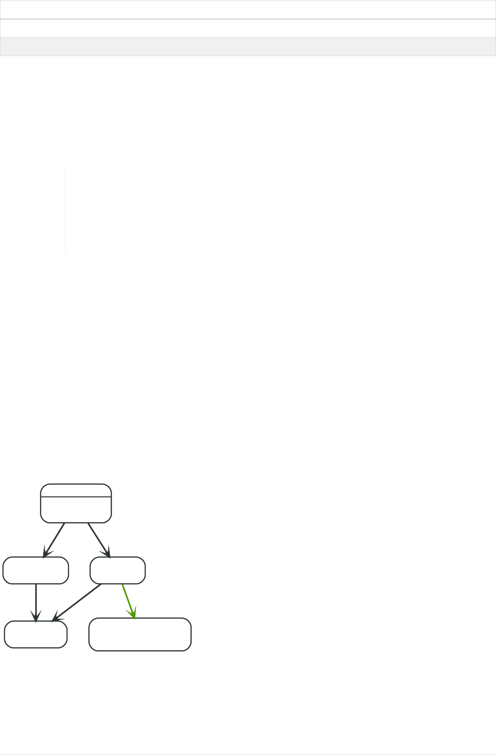
Table 255. Result
sum(dur)
P2DT4H45S
1 row
4.4. List functions
List functions return lists of things — nodes in a path, and so on.
Further details and examples of lists may be found in Lists and List operators.
The function rels() has been superseded by relationships(), and will be removed
in a future release.
The functions extract() and filter() have been deprecated and will be removed in
a future release. Consider using a list comprehension (e.g. [x IN xs WHERE
predicate | extraction]) instead.
Functions:
•extract()
•filter()
•keys()
•labels()
•nodes()
•range()
•reduce()
•relationships()
•reverse()
•tail()
Person, Developer
name = 'Alice'
eyes = 'brown'
age = 38
name = 'Charlie'
eyes = 'green'
age = 53
KNOWS
name = 'Bob'
eyes = 'blue'
age = 25
KNOWS
name = 'Daniel'
eyes = 'brown'
age = 54
KNOWS
array = ['one', 'two', 'three']
name = 'Eskil'
eyes = 'blue'
age = 41
MARRIEDKNOWS
Figure 25. Graph
4.4.1. extract()
extract() returns a list lresult containing the values resulting from an expression which has been
186

applied to each element in a list list. This function is analogous to the map method in functional
languages such as Lisp and Scala. Note that this function has been deprecated, consider using a list
comprehension (e.g. [variable IN list | expression]) instead.
Syntax: extract(variable IN list | expression)
Returns:
A list containing heterogeneous elements; the types of the elements are determined by expression.
Arguments:
Name Description
list An expression that returns a list.
variable The closure will have a variable introduced in its context.
We decide here which variable to use.
expression This expression will run once per value in list, and add it
to the list which is returned by extract().
Considerations:
Any null values in list are preserved.
Common usages of extract() include:
•Returning a property from a list of nodes or relationships; for example, expression = n.prop and
list = nodes(<some-path>).
•Returning the result of the application of a function on each element in a list; for example,
expression = toUpper(x) and variable = x.
Query
MATCH p =(a)-->(b)-->(c)
WHERE a.name = 'Alice' AND b.name = 'Bob' AND c.name = 'Daniel'
RETURN extract(n IN nodes(p)| n.age) AS extracted
The age property of all nodes in path p are returned.
Table 256. Result
extracted
[38,25,54]
1 row
4.4.2. filter()
filter() returns a list lresult containing all the elements from a list list that comply with the given
predicate. Note that this function has been deprecated, consider using a list comprehension (e.g.
[variable IN list WHERE predicate]) instead.
Syntax: filter(variable IN list WHERE predicate)
Returns:
A list containing heterogeneous elements; the types of the elements are determined by the elements in list.
187

Arguments:
Name Description
list An expression that returns a list.
variable This is the variable that can be used from the predicate.
predicate A predicate that is tested against all elements in list.
Query
MATCH (a)
WHERE a.name = 'Eskil'
RETURN a.array, filter(x IN a.array WHERE size(x)= 3)
The property named array and a list of all values having size '3' are returned.
Table 257. Result
a.array filter(x IN a.array WHERE size(x)= 3)
["one","two","three"] ["one","two"]
1 row
4.4.3. keys()
keys returns a list containing the string representations for all the property names of a node,
relationship, or map.
Syntax: keys(expression)
Returns:
A list containing String elements.
Arguments:
Name Description
expression An expression that returns a node, a relationship, or a
map.
Considerations:
keys(null) returns null.
Query
MATCH (a)
WHERE a.name = 'Alice'
RETURN keys(a)
A list containing the names of all the properties on the node bound to a is returned.
Table 258. Result
keys(a)
["name","eyes","age"]
188

keys(a)
1 row
4.4.4. labels()
labels returns a list containing the string representations for all the labels of a node.
Syntax: labels(node)
Returns:
A list containing String elements.
Arguments:
Name Description
node An expression that returns a single node.
Considerations:
labels(null) returns null.
Query
MATCH (a)
WHERE a.name = 'Alice'
RETURN labels(a)
A list containing all the labels of the node bound to a is returned.
Table 259. Result
labels(a)
["Person","Developer"]
1 row
4.4.5. nodes()
nodes() returns a list containing all the nodes in a path.
Syntax: nodes(path)
Returns:
A list containing Node elements.
Arguments:
Name Description
path An expression that returns a path.
Considerations:
189

nodes(null) returns null.
Query
MATCH p =(a)-->(b)-->(c)
WHERE a.name = 'Alice' AND c.name = 'Eskil'
RETURN nodes(p)
A list containing all the nodes in the path p is returned.
Table 260. Result
nodes(p)
[Node[0]{name:"Alice",eyes:"brown",age:38},Node[1]{name:"Bob",eyes:"blue",age:25},Node[4]{array:["one","two","
three"],name:"Eskil",eyes:"blue",age:41}]
1 row
4.4.6. range()
range() returns a list comprising all integer values within a range bounded by a start value start and
end value end, where the difference step between any two consecutive values is constant; i.e. an
arithmetic progression. The range is inclusive, and the arithmetic progression will therefore always
contain start and — depending on the values of start, step and end — end.
Syntax: range(start, end [, step])
Returns:
A list of Integer elements.
Arguments:
Name Description
start An expression that returns an integer value.
end An expression that returns an integer value.
step A numeric expression defining the difference between any
two consecutive values, with a default of 1.
Query
RETURN range(0, 10), range(2, 18, 3)
Two lists of numbers in the given ranges are returned.
Table 261. Result
range(0, 10) range(2, 18, 3)
[0,1,2,3,4,5,6,7,8,9,10] [2,5,8,11,14,17]
1 row
4.4.7. reduce()
reduce() returns the value resulting from the application of an expression on each successive element
in a list in conjunction with the result of the computation thus far. This function will iterate
190

through each element e in the given list, run the expression on e — taking into account the current
partial result — and store the new partial result in the accumulator. This function is analogous
to the fold or reduce method in functional languages such as Lisp and Scala.
Syntax: reduce(accumulator = initial, variable IN list | expression)
Returns:
The type of the value returned depends on the arguments provided, along with the semantics of expression.
Arguments:
Name Description
accumulator A variable that will hold the result and the partial results as
the list is iterated.
initial An expression that runs once to give a starting value to the
accumulator.
list An expression that returns a list.
variable The closure will have a variable introduced in its context.
We decide here which variable to use.
expression This expression will run once per value in the list, and
produce the result value.
Query
MATCH p =(a)-->(b)-->(c)
WHERE a.name = 'Alice' AND b.name = 'Bob' AND c.name = 'Daniel'
RETURN reduce(totalAge = 0, n IN nodes(p)| totalAge + n.age) AS reduction
The age property of all nodes in the path are summed and returned as a single value.
Table 262. Result
reduction
117
1 row
4.4.8. relationships()
relationships() returns a list containing all the relationships in a path.
Syntax: relationships(path)
Returns:
A list containing Relationship elements.
Arguments:
Name Description
path An expression that returns a path.
Considerations:
191

relationships(null) returns null.
Query
MATCH p =(a)-->(b)-->(c)
WHERE a.name = 'Alice' AND c.name = 'Eskil'
RETURN relationships(p)
A list containing all the relationships in the path p is returned.
Table 263. Result
relationships(p)
[:KNOWS[0]{},:MARRIED[4]{}]
1 row
4.4.9. reverse()
reverse() returns a list in which the order of all elements in the original list have been reversed.
Syntax: reverse(original)
Returns:
A list containing homogeneous or heterogeneous elements; the types of the elements are determined by the elements
within original.
Arguments:
Name Description
original An expression that returns a list.
Considerations:
Any null element in original is preserved.
Query
WITH [4923,'abc',521, NULL , 487] AS ids
RETURN reverse(ids)
Table 264. Result
reverse(ids)
[487,<null>,521,"abc",4923]
1 row
4.4.10. tail()
tail() returns a list lresult containing all the elements, excluding the first one, from a list list.
Syntax: tail(list)
Returns:
192

A list containing heterogeneous elements; the types of the elements are determined by the elements in list.
Arguments:
Name Description
list An expression that returns a list.
Query
MATCH (a)
WHERE a.name = 'Eskil'
RETURN a.array, tail(a.array)
The property named array and a list comprising all but the first element of the array property are
returned.
Table 265. Result
a.array tail(a.array)
["one","two","three"] ["two","three"]
1 row
4.5. Mathematical functions - numeric
These functions all operate on numeric expressions only, and will return an error if used on
any other values. See also Mathematical operators.
Functions:
•abs()
•ceil()
•floor()
•rand()
•round()
•sign()
The following graph is used for the examples below:
193
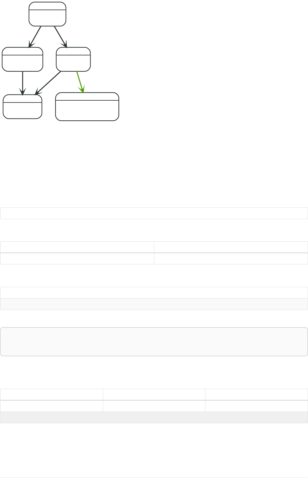
A
name = 'Alice'
eyes = 'brown'
age = 38
C
name = 'Charlie'
eyes = 'green'
age = 53
KNOWS
B
name = 'Bob'
eyes = 'blue'
age = 25
KNOWS
D
name = 'Daniel'
eyes = 'brown'
age = 54
KNOWS
E
array = ['one', 'two', 'three']
name = 'Eskil'
eyes = 'blue'
age = 41
MARRIEDKNOWS
Figure 26. Graph
4.5.1. abs()
abs() returns the absolute value of the given number.
Syntax: abs(expression)
Returns:
The type of the value returned will be that of expression.
Arguments:
Name Description
expression A numeric expression.
Considerations:
abs(null) returns null.
If expression is negative, -(expression) (i.e. the negation of expression) is returned.
Query
MATCH (a),(e)
WHERE a.name = 'Alice' AND e.name = 'Eskil'
RETURN a.age, e.age, abs(a.age - e.age)
The absolute value of the age difference is returned.
Table 266. Result
a.age e.age abs(a.age - e.age)
38 41 3
1 row
4.5.2. ceil()
ceil() returns the smallest floating point number that is greater than or equal to the given number
and equal to a mathematical integer.
194

Syntax: ceil(expression)
Returns:
A Float.
Arguments:
Name Description
expression A numeric expression.
Considerations:
ceil(null) returns null.
Query
RETURN ceil(0.1)
The ceil of 0.1 is returned.
Table 267. Result
ceil(0.1)
1.0
1 row
4.5.3. floor()
floor() returns the largest floating point number that is less than or equal to the given number and
equal to a mathematical integer.
Syntax: floor(expression)
Returns:
A Float.
Arguments:
Name Description
expression A numeric expression.
Considerations:
floor(null) returns null.
Query
RETURN floor(0.9)
The floor of 0.9 is returned.
Table 268. Result
195

floor(0.9)
0.0
1 row
4.5.4. rand()
rand() returns a random floating point number in the range from 0 (inclusive) to 1 (exclusive); i.e.
[0,1). The numbers returned follow an approximate uniform distribution.
Syntax: rand()
Returns:
A Float.
Query
RETURN rand()
A random number is returned.
Table 269. Result
rand()
0.9388741209942687
1 row
4.5.5. round()
round() returns the value of the given number rounded to the nearest integer.
Syntax: round(expression)
Returns:
A Float.
Arguments:
Name Description
expression A numeric expression.
Considerations:
round(null) returns null.
Query
RETURN round(3.141592)
3.0 is returned.
Table 270. Result
196

round(3.141592)
3.0
1 row
4.5.6. sign()
sign() returns the signum of the given number: 0 if the number is 0, -1 for any negative number, and
1 for any positive number.
Syntax: sign(expression)
Returns:
An Integer.
Arguments:
Name Description
expression A numeric expression.
Considerations:
sign(null) returns null.
Query
RETURN sign(-17), sign(0.1)
The signs of -17 and 0.1 are returned.
Table 271. Result
sign(-17) sign(0.1)
-1 1
1 row
4.6. Mathematical functions - logarithmic
These functions all operate on numeric expressions only, and will return an error if used on
any other values. See also Mathematical operators.
Functions:
•e()
•exp()
•log()
•log10()
•sqrt()
197

4.6.1. e()
e() returns the base of the natural logarithm, e.
Syntax: e()
Returns:
A Float.
Query
RETURN e()
The base of the natural logarithm, e, is returned.
Table 272. Result
e()
2.718281828459045
1 row
4.6.2. exp()
exp() returns e^n, where e is the base of the natural logarithm, and n is the value of the argument
expression.
Syntax: e(expression)
Returns:
A Float.
Arguments:
Name Description
expression A numeric expression.
Considerations:
exp(null) returns null.
Query
RETURN exp(2)
e to the power of 2 is returned.
Table 273. Result
exp(2)
7.38905609893065
1 row
198

4.6.3. log()
log() returns the natural logarithm of a number.
Syntax: log(expression)
Returns:
A Float.
Arguments:
Name Description
expression A numeric expression.
Considerations:
log(null) returns null.
log(0) returns null.
Query
RETURN log(27)
The natural logarithm of 27 is returned.
Table 274. Result
log(27)
3.295836866004329
1 row
4.6.4. log10()
log10() returns the common logarithm (base 10) of a number.
Syntax: log10(expression)
Returns:
A Float.
Arguments:
Name Description
expression A numeric expression.
Considerations:
log10(null) returns null.
log10(0) returns null.
199

Query
RETURN log10(27)
The common logarithm of 27 is returned.
Table 275. Result
log10(27)
1.4313637641589874
1 row
4.6.5. sqrt()
sqrt() returns the square root of a number.
Syntax: sqrt(expression)
Returns:
A Float.
Arguments:
Name Description
expression A numeric expression.
Considerations:
sqrt(null) returns null.
sqrt(<any negative number>) returns null
Query
RETURN sqrt(256)
The square root of 256 is returned.
Table 276. Result
sqrt(256)
16.0
1 row
4.7. Mathematical functions - trigonometric
These functions all operate on numeric expressions only, and will return an error if used on
any other values. See also Mathematical operators.
Functions:
•acos()
200

•asin()
•atan()
•atan2()
•cos()
•cot()
•degrees()
•haversin()
•Spherical distance using the haversin() function
•pi()
•radians()
•sin()
•tan()
4.7.1. acos()
acos() returns the arccosine of a number in radians.
Syntax: acos(expression)
Returns:
A Float.
Arguments:
Name Description
expression A numeric expression that represents the angle in radians.
Considerations:
acos(null) returns null.
If (expression < -1) or (expression > 1), then (acos(expression)) returns null.
Query
RETURN acos(0.5)
The arccosine of 0.5 is returned.
Table 277. Result
acos(0.5)
1.0471975511965979
1 row
4.7.2. asin()
asin() returns the arcsine of a number in radians.
Syntax: asin(expression)
201

Returns:
A Float.
Arguments:
Name Description
expression A numeric expression that represents the angle in radians.
Considerations:
asin(null) returns null.
If (expression < -1) or (expression > 1), then (asin(expression)) returns null.
Query
RETURN asin(0.5)
The arcsine of 0.5 is returned.
Table 278. Result
asin(0.5)
0.5235987755982989
1 row
4.7.3. atan()
atan() returns the arctangent of a number in radians.
Syntax: atan(expression)
Returns:
A Float.
Arguments:
Name Description
expression A numeric expression that represents the angle in radians.
Considerations:
atan(null) returns null.
Query
RETURN atan(0.5)
The arctangent of 0.5 is returned.
Table 279. Result
202

atan(0.5)
0.4636476090008061
1 row
4.7.4. atan2()
atan2() returns the arctangent2 of a set of coordinates in radians.
Syntax: atan2(expression1, expression2)
Returns:
A Float.
Arguments:
Name Description
expression1 A numeric expression for y that represents the angle in
radians.
expression2 A numeric expression for x that represents the angle in
radians.
Considerations:
atan2(null, null), atan2(null, expression2) and atan(expression1, null) all return null.
Query
RETURN atan2(0.5, 0.6)
The arctangent2 of 0.5 and 0.6 is returned.
Table 280. Result
atan2(0.5, 0.6)
0.6947382761967033
1 row
4.7.5. cos()
cos() returns the cosine of a number.
Syntax: cos(expression)
Returns:
A Float.
Arguments:
Name Description
expression A numeric expression that represents the angle in radians.
203

Considerations:
cos(null) returns null.
Query
RETURN cos(0.5)
The cosine of 0.5 is returned.
Table 281. Result
cos(0.5)
0.8775825618903728
1 row
4.7.6. cot()
cot() returns the cotangent of a number.
Syntax: cot(expression)
Returns:
A Float.
Arguments:
Name Description
expression A numeric expression that represents the angle in radians.
Considerations:
cot(null) returns null.
cot(0) returns null.
Query
RETURN cot(0.5)
The cotangent of 0.5 is returned.
Table 282. Result
cot(0.5)
1.830487721712452
1 row
4.7.7. degrees()
degrees() converts radians to degrees.
Syntax: degrees(expression)
204

Returns:
A Float.
Arguments:
Name Description
expression A numeric expression that represents the angle in radians.
Considerations:
degrees(null) returns null.
Query
RETURN degrees(3.14159)
The number of degrees in something close to pi is returned.
Table 283. Result
degrees(3.14159)
179.99984796050427
1 row
4.7.8. haversin()
haversin() returns half the versine of a number.
Syntax: haversin(expression)
Returns:
A Float.
Arguments:
Name Description
expression A numeric expression that represents the angle in radians.
Considerations:
haversin(null) returns null.
Query
RETURN haversin(0.5)
The haversine of 0.5 is returned.
Table 284. Result
haversin(0.5)
0.06120871905481362
205

haversin(0.5)
1 row
4.7.9. Spherical distance using the haversin() function
The haversin() function may be used to compute the distance on the surface of a sphere between
two points (each given by their latitude and longitude). In this example the spherical distance (in km)
between Berlin in Germany (at lat 52.5, lon 13.4) and San Mateo in California (at lat 37.5, lon -122.3) is
calculated using an average earth radius of 6371 km.
Query
CREATE (ber:City { lat: 52.5, lon: 13.4 }),(sm:City { lat: 37.5, lon: -122.3 })
RETURN 2 * 6371 * asin(sqrt(haversin(radians(sm.lat - ber.lat))+ cos(radians(sm.lat))*
cos(radians(ber.lat))* haversin(radians(sm.lon - ber.lon)))) AS dist
The estimated distance between 'Berlin' and 'San Mateo' is returned.
Table 285. Result
dist
9129.969740051658
1 row
Nodes created: 2
Properties set: 4
Labels added: 2
4.7.10. pi()
pi() returns the mathematical constant pi.
Syntax: pi()
Returns:
A Float.
Query
RETURN pi()
The constant pi is returned.
Table 286. Result
pi()
3.141592653589793
1 row
4.7.11. radians()
radians() converts degrees to radians.
Syntax: radians(expression)
206

Returns:
A Float.
Arguments:
Name Description
expression A numeric expression that represents the angle in degrees.
Considerations:
radians(null) returns null.
Query
RETURN radians(180)
The number of radians in 180 degrees is returned (pi).
Table 287. Result
radians(180)
3.141592653589793
1 row
4.7.12. sin()
sin() returns the sine of a number.
Syntax: sin(expression)
Returns:
A Float.
Arguments:
Name Description
expression A numeric expression that represents the angle in radians.
Considerations:
sin(null) returns null.
Query
RETURN sin(0.5)
The sine of 0.5 is returned.
Table 288. Result
sin(0.5)
0.479425538604203
207

sin(0.5)
1 row
4.7.13. tan()
tan() returns the tangent of a number.
Syntax: tan(expression)
Returns:
A Float.
Arguments:
Name Description
expression A numeric expression that represents the angle in radians.
Considerations:
tan(null) returns null.
Query
RETURN tan(0.5)
The tangent of 0.5 is returned.
Table 289. Result
tan(0.5)
0.5463024898437905
1 row
4.8. String functions
These functions all operate on string expressions only, and will return an error if used on any
other values. The exception to this rule is toString(), which also accepts numbers, booleans
and temporal values (i.e. Date, Time. LocalTime, DateTime, LocalDateTime or Duration
values).
Functions taking a string as input all operate on Unicode characters rather than on a standard char[].
For example, size(s), where s is a character in the Chinese alphabet, will return 1.
The functions lower() and upper() have been superseded by toLower() and
toUpper(), respectively, and will be removed in a future release.
When toString() is applied to a temporal value, it returns a string representation
suitable for parsing by the corresponding temporal functions. This string will
therefore be formatted according to the ISO 8601 (https://en.wikipedia.org/wiki/ISO_8601)
format.
208

See also String operators.
Functions:
•left()
•lTrim()
•replace()
•reverse()
•right()
•rTrim()
•split()
•substring()
•toLower()
•toString()
•toUpper()
•trim()
4.8.1. left()
left() returns a string containing the specified number of leftmost characters of the original string.
Syntax: left(original, length)
Returns:
A String.
Arguments:
Name Description
original An expression that returns a string.
nAn expression that returns a positive integer.
Considerations:
left(null, length) and left(null, null) both return null
left(original, null) will raise an error.
If length is not a positive integer, an error is raised.
If length exceeds the size of original, original is returned.
Query
RETURN left('hello', 3)
Table 290. Result
left('hello', 3)
"hel"
1 row
209

4.8.2. ltrim()
lTrim() returns the original string with leading whitespace removed.
Syntax: lTrim(original)
Returns:
A String.
Arguments:
Name Description
original An expression that returns a string.
Considerations:
lTrim(null) returns null
Query
RETURN lTrim(' hello')
Table 291. Result
lTrim(' hello')
"hello"
1 row
4.8.3. replace()
replace() returns a string in which all occurrences of a specified string in the original string have been
replaced by another (specified) string.
Syntax: replace(original, search, replace)
Returns:
A String.
Arguments:
Name Description
original An expression that returns a string.
search An expression that specifies the string to be replaced in
original.
replace An expression that specifies the replacement string.
Considerations:
If any argument is null, null will be returned.
If search is not found in original, original will be returned.
210

Query
RETURN replace("hello", "l", "w")
Table 292. Result
replace("hello", "l", "w")
"hewwo"
1 row
4.8.4. reverse()
reverse() returns a string in which the order of all characters in the original string have been reversed.
Syntax: reverse(original)
Returns:
A String.
Arguments:
Name Description
original An expression that returns a string.
Considerations:
reverse(null) returns null.
Query
RETURN reverse('anagram')
Table 293. Result
reverse('anagram')
"margana"
1 row
4.8.5. right()
right() returns a string containing the specified number of rightmost characters of the original string.
Syntax: right(original, length)
Returns:
A String.
Arguments:
Name Description
original An expression that returns a string.
211

Name Description
nAn expression that returns a positive integer.
Considerations:
right(null, length) and right(null, null) both return null
right(original, null) will raise an error.
If length is not a positive integer, an error is raised.
If length exceeds the size of original, original is returned.
Query
RETURN right('hello', 3)
Table 294. Result
right('hello', 3)
"llo"
1 row
4.8.6. rtrim()
rTrim() returns the original string with trailing whitespace removed.
Syntax: rTrim(original)
Returns:
A String.
Arguments:
Name Description
original An expression that returns a string.
Considerations:
rTrim(null) returns null
Query
RETURN rTrim('hello ')
Table 295. Result
rTrim('hello ')
"hello"
1 row
212

4.8.7. split()
split() returns a list of strings resulting from the splitting of the original string around matches of the
given delimiter.
Syntax: split(original, splitDelimiter)
Returns:
A list of Strings.
Arguments:
Name Description
original An expression that returns a string.
splitDelimiter The string with which to split original.
Considerations:
split(null, splitDelimiter) and split(original, null) both return null
Query
RETURN split('one,two', ',')
Table 296. Result
split('one,two', ',')
["one","two"]
1 row
4.8.8. substring()
substring() returns a substring of the original string, beginning with a 0-based index start and length.
Syntax: substring(original, start [, length])
Returns:
A String.
Arguments:
Name Description
original An expression that returns a string.
start An expression that returns a positive integer, denoting the
position at which the substring will begin.
length An expression that returns a positive integer, denoting
how many characters of original will be returned.
Considerations:
start uses a zero-based index.
213

If length is omitted, the function returns the substring starting at the position given by start and extending to the end
of original.
If original is null, null is returned.
If either start or length is null or a negative integer, an error is raised.
If start is 0, the substring will start at the beginning of original.
If length is 0, the empty string will be returned.
Query
RETURN substring('hello', 1, 3), substring('hello', 2)
Table 297. Result
substring('hello', 1, 3) substring('hello', 2)
"ell" "llo"
1 row
4.8.9. toLower()
toLower() returns the original string in lowercase.
Syntax: toLower(original)
Returns:
A String.
Arguments:
Name Description
original An expression that returns a string.
Considerations:
toLower(null) returns null
Query
RETURN toLower('HELLO')
Table 298. Result
toLower('HELLO')
"hello"
1 row
4.8.10. toString()
toString() converts an integer, float or boolean value to a string.
Syntax: toString(expression)
214

Returns:
A String.
Arguments:
Name Description
expression An expression that returns a number, a boolean, or a
string.
Considerations:
toString(null) returns null
If expression is a string, it will be returned unchanged.
Query
RETURN toString(11.5), toString('already a string'), toString(TRUE ), toString(date({ year:1984, month:10,
day:11 })) AS dateString, toString(datetime({ year:1984, month:10, day:11, hour:12, minute:31, second:14,
millisecond: 341, timezone: 'Europe/Stockholm' })) AS datetimeString, toString(duration({ minutes: 12,
seconds: -60 })) AS durationString
Table 299. Result
toString(11.5) toString('already
a string')
toString(TRUE ) dateString datetimeString durationString
"11.5" "already a
string"
"true" "1984-10-11" "1984-10-
11T12:31:14.341+0
1:00[Europe/Stock
holm]"
"PT11M"
1 row
4.8.11. toUpper()
toUpper() returns the original string in uppercase.
Syntax: toUpper(original)
Returns:
A String.
Arguments:
Name Description
original An expression that returns a string.
Considerations:
toUpper(null) returns null
Query
RETURN toUpper('hello')
Table 300. Result
215

toUpper('hello')
"HELLO"
1 row
4.8.12. trim()
trim() returns the original string with leading and trailing whitespace removed.
Syntax: trim(original)
Returns:
A String.
Arguments:
Name Description
original An expression that returns a string.
Considerations:
trim(null) returns null
Query
RETURN trim(' hello ')
Table 301. Result
trim(' hello ')
"hello"
1 row
4.9. Temporal functions - instant types
Cypher provides functions allowing for the creation and manipulation of values for each
temporal type — Date, Time, LocalTime, DateTime, and LocalDateTime.
See also Temporal (Date/Time) values and Temporal operators.
Temporal instant types
•An overview of temporal instant type creation
•Controlling which clock to use
•Truncating temporal values
Functions:
•date()
•Getting the current Date
216

•Creating a calendar (Year-Month-Day) Date
•Creating a week (Year-Week-Day) Date
•Creating a quarter (Year-Quarter-Day) Date
•Creating an ordinal (Year-Day) Date
•Creating a Date from a string
•Creating a Date using other temporal values as components
•Truncating a Date
•datetime()
•Getting the current DateTime
•Creating a calendar (Year-Month-Day) DateTime
•Creating a week (Year-Week-Day) DateTime
•Creating a quarter (Year-Quarter-Day) DateTime
•Creating an ordinal (Year-Day) DateTime
•Creating a DateTime from a string
•Creating a DateTime using other temporal values as components
•Creating a DateTime from a timestamp
•Truncating a DateTime
•localdatetime()
•Getting the current LocalDateTime
•Creating a calendar (Year-Month-Day) LocalDateTime
•Creating a week (Year-Week-Day) LocalDateTime
•Creating a quarter (Year-Quarter-Day) DateTime
•Creating an ordinal (Year-Day) LocalDateTime
•Creating a LocalDateTime from a string
•Creating a LocalDateTime using other temporal values as components
•Truncating a LocalDateTime
•localtime()
•Getting the current LocalTime
•Creating a LocalTime
•Creating a LocalTime from a string
•Creating a LocalTime using other temporal values as components
•Truncating a LocalTime
•time()
•Getting the current Time
•Creating a Time
•Creating a Time from a string
•Creating a Time using other temporal values as components
•Truncating a Time
217

4.9.1. Temporal instant types
An introduction to temporal instant types, including descriptions of creation functions,
clocks, and truncation.
An overview of temporal instant type creation
Each function bears the same name as the type, and construct the type they correspond to in one of
four ways:
•Capturing the current time
•Composing the components of the type
•Parsing a string representation of the temporal value
•Selecting and composing components from another temporal value by
•either combining temporal values (such as combining a Date with a Time to create a DateTime),
or
•selecting parts from a temporal value (such as selecting the Date from a DateTime); the
extractors — groups of components which can be selected — are:
•date — contains all components for a Date (conceptually year, month and day).
•time — contains all components for a Time (hour, minute, second, and sub-seconds; namely
millisecond, microsecond and nanosecond). If the type being created and the type from
which the time component is being selected both contain timezone (and a timezone is not
explicitly specified) the timezone is also selected.
•datetime — selects all components, and is useful for overriding specific components.
Analogously to time, if the type being created and the type from which the time component
is being selected both contain timezone (and a timezone is not explicitly specified) the
timezone is also selected.
•In effect, this allows for the conversion between different temporal types, and allowing for
'missing' components to be specified.
Table 302. Temporal instant type creation functions
Function Date Time LocalTime DateTime LocalDateTime
Getting the
current value
XXXXX
Creating a
calendar-based
(Year-Month-Day)
value
X X X
Creating a week-
based (Year-Week-
Day) value
X X X
Creating a
quarter-based
(Year-Quarter-Day)
value
X X X
Creating an
ordinal (Year-Day)
value
X X X
Creating a value
from time
components
X X
218

Function Date Time LocalTime DateTime LocalDateTime
Creating a value
from other
temporal values
using extractors
(i.e. converting
between different
types)
XXXXX
Creating a value
from a string
XXXXX
Creating a value
from a timestamp
X
All the temporal instant types — including those that do not contain time zone
information support such as Date, LocalTime and DateTime — allow for a time zone
to specified for the functions that retrieve the current instant. This allows for the
retrieval of the current instant in the specified time zone.
Controlling which clock to use
The functions which create temporal instant values based on the current instant use the statement
clock as default. However, there are three different clocks available for more fine-grained control:
•transaction: The same instant is produced for each invocation within the same transaction. A
different time may be produced for different transactions.
•statement: The same instant is produced for each invocation within the same statement. A
different time may be produced for different statements within the same transaction.
•realtime: The instant produced will be the live clock of the system.
The following table lists the different sub-functions for specifying the clock to be used when creating
the current temporal instant value:
Type default transaction statement realtime
Date date() date.transaction() date.statement() date.realtime()
Time time() time.transaction() time.statement() time.realtime()
LocalTime localtime() localtime.transaction() localtime.statement() localtime.realtime()
DateTime datetime() datetime.transaction() datetime.statement() datetime.realtime()
LocalDateTime localdatetime() localdatetime.transact
ion()
localdatetime.stateme
nt()
localdatetime.realtime
()
Truncating temporal values
A temporal instant value can be created by truncating another temporal instant value at the nearest
preceding point in time at a specified component boundary (namely, a truncation unit). A temporal
instant value created in this way will have all components which are less significant than the specified
truncation unit set to their default values.
It is possible to supplement the truncated value by providing a map containing components which are
less significant than the truncation unit. This will have the effect of overriding the default values which
would otherwise have been set for these less significant components.
The following truncation units are supported:
•millennium: Select the temporal instant corresponding to the millenium of the given instant.
219
•century: Select the temporal instant corresponding to the century of the given instant.
•decade: Select the temporal instant corresponding to the decade of the given instant.
•year: Select the temporal instant corresponding to the year of the given instant.
•weekYear: Select the temporal instant corresponding to the first day of the first week of the week-
year of the given instant.
•quarter: Select the temporal instant corresponding to the quarter of the year of the given instant.
•month: Select the temporal instant corresponding to the month of the given instant.
•week: Select the temporal instant corresponding to the week of the given instant.
•day: Select the temporal instant corresponding to the month of the given instant.
•hour: Select the temporal instant corresponding to the hour of the given instant.
•minute: Select the temporal instant corresponding to the minute of the given instant.
•second: Select the temporal instant corresponding to the second of the given instant.
•millisecond: Select the temporal instant corresponding to the millisecond of the given instant.
•microsecond: Select the temporal instant corresponding to the microsecond of the given instant.
The following table lists the supported truncation units and the corresponding sub-functions:
Truncation unit Date Time LocalTime DateTime LocalDateTime
millennium date.truncate('mill
ennium', input)
datetime.truncate(
'millennium',
input)
localdatetime.trun
cate('millennium',
input)
century date.truncate('cen
tury', input)
datetime.truncate(
'century', input)
localdatetime.trun
cate('century',
input)
decade date.truncate('dec
ade', input)
datetime.truncate(
'decade', input)
localdatetime.trun
cate('decade',
input)
year date.truncate('yea
r', input)
datetime.truncate(
'year', input)
localdatetime.trun
cate('year', input)
weekYear date.truncate('wee
kYear', input)
datetime.truncate(
'weekYear', input)
localdatetime.trun
cate('weekYear',
input)
quarter date.truncate('qua
rter', input)
datetime.truncate(
'quarter', input)
localdatetime.trun
cate('quarter',
input)
month date.truncate('mo
nth', input)
datetime.truncate(
'month', input)
localdatetime.trun
cate('month',
input)
week date.truncate('wee
k', input)
datetime.truncate(
'week', input)
localdatetime.trun
cate('week', input)
day date.truncate('day'
, input)
time.truncate('day'
, input)
localtime.truncate(
'day', input)
datetime.truncate(
'day', input)
localdatetime.trun
cate('day', input)
hour time.truncate('hou
r', input)
localtime.truncate(
'hour', input)
datetime.truncate(
'hour', input)
localdatetime.trun
cate('hour',input)
minute time.truncate('min
ute', input)
localtime.truncate(
'minute', input)
datetime.truncate(
'minute', input)
localdatetime.trun
cate('minute',
input)
second time.truncate('sec
ond', input)
localtime.truncate(
'second', input)
datetime.truncate(
'second', input)
localdatetime.trun
cate('second',
input)
220

Truncation unit Date Time LocalTime DateTime LocalDateTime
millisecond time.truncate('milli
second', input)
localtime.truncate(
'millisecond',
input)
datetime.truncate(
'millisecond',
input)
localdatetime.trun
cate('millisecond',
input)
microsecond time.truncate('mic
rosecond', input)
localtime.truncate(
'microsecond',
input)
datetime.truncate(
'microsecond',
input)
localdatetime.trun
cate('microsecond'
, input)
4.9.2. Date: date()
Details for using the date() function.
•Getting the current Date
•Creating a calendar (Year-Month-Day) Date
•Creating a week (Year-Week-Day) Date
•Creating a quarter (Year-Quarter-Day) Date
•Creating an ordinal (Year-Day) Date
•Creating a Date from a string
•Creating a Date using other temporal values as components
•Truncating a Date
Getting the current Date
date() returns the current Date value. If no time zone parameter is specified, the local time zone will
be used.
Syntax: date([ {timezone} ])
Returns:
A Date.
Arguments:
Name Description
A single map consisting of the following:
timezone A string expression that represents the time zone
Considerations:
If no parameters are provided, date() must be invoked (date({}) is invalid).
Query
RETURN date() AS currentDate
The current date is returned.
Table 303. Result
221

currentDate
2018-12-10
1 row
Query
RETURN date({ timezone: 'America/Los Angeles' }) AS currentDateInLA
The current date in California is returned.
Table 304. Result
currentDateInLA
2018-12-10
1 row
date.transaction()
date.transaction() returns the current Date value using the transaction clock. This value will be the
same for each invocation within the same transaction. However, a different value may be produced
for different transactions.
Syntax: date.transaction([ {timezone} ])
Returns:
A Date.
Arguments:
Name Description
timezone A string expression that represents the time zone
Query
RETURN date.transaction() AS currentDate
Table 305. Result
currentDate
2018-12-10
1 row
date.statement()
date.statement() returns the current Date value using the statement clock. This value will be the same
for each invocation within the same statement. However, a different value may be produced for
different statements within the same transaction.
Syntax: date.statement([ {timezone} ])
Returns:
A Date.
222

Arguments:
Name Description
timezone A string expression that represents the time zone
Query
RETURN date.statement() AS currentDate
Table 306. Result
currentDate
2018-12-10
1 row
date.realtime()
date.realtime() returns the current Date value using the realtime clock. This value will be the live
clock of the system.
Syntax: date.realtime([ {timezone} ])
Returns:
A Date.
Arguments:
Name Description
timezone A string expression that represents the time zone
Query
RETURN date.realtime() AS currentDate
Table 307. Result
currentDate
2018-12-10
1 row
Query
RETURN date.realtime('America/Los Angeles') AS currentDateInLA
Table 308. Result
currentDateInLA
2018-12-10
1 row
223

Creating a calendar (Year-Month-Day) Date
date() returns a Date value with the specified year, month and day component values.
Syntax: date({year [, month, day]})
Returns:
A Date.
Arguments:
Name Description
A single map consisting of the following:
year An expression consisting of at least four digits that
specifies the year.
month An integer between 1 and 12 that specifies the month.
day An integer between 1 and 31 that specifies the day of the
month.
Considerations:
The day of the month component will default to 1 if day is omitted.
The month component will default to 1 if month is omitted.
If month is omitted, day must also be omitted.
Query
UNWIND [
date({ year:1984, month:10, day:11 }),
date({ year:1984, month:10 }),
date({ year:1984 })
] AS theDate
RETURN theDate
Table 309. Result
theDate
1984-10-11
1984-10-01
1984-01-01
3 rows
Creating a week (Year-Week-Day) Date
date() returns a Date value with the specified year, week and dayOfWeek component values.
Syntax: date({year [, week, dayOfWeek]})
Returns:
A Date.
Arguments:
224

Name Description
A single map consisting of the following:
year An expression consisting of at least four digits that
specifies the year.
week An integer between 1 and 53 that specifies the week.
dayOfWeek An integer between 1 and 7 that specifies the day of the
week.
Considerations:
The day of the week component will default to 1 if dayOfWeek is omitted.
The week component will default to 1 if week is omitted.
If week is omitted, dayOfWeek must also be omitted.
Query
UNWIND [
date({ year:1984, week:10, dayOfWeek:3 }),
date({ year:1984, week:10 }),
date({ year:1984 })
] AS theDate
RETURN theDate
Table 310. Result
theDate
1984-03-07
1984-03-05
1984-01-01
3 rows
Creating a quarter (Year-Quarter-Day) Date
date() returns a Date value with the specified year, quarter and dayOfQuarter component values.
Syntax: date({year [, quarter, dayOfQuarter]})
Returns:
A Date.
Arguments:
Name Description
A single map consisting of the following:
year An expression consisting of at least four digits that
specifies the year.
quarter An integer between 1 and 4 that specifies the quarter.
dayOfQuarter An integer between 1 and 92 that specifies the day of the
quarter.
Considerations:
225

The day of the quarter component will default to 1 if dayOfQuarter is omitted.
The quarter component will default to 1 if quarter is omitted.
If quarter is omitted, dayOfQuarter must also be omitted.
Query
UNWIND [
date({ year:1984, quarter:3, dayOfQuarter: 45 }),
date({ year:1984, quarter:3 }),
date({ year:1984 })
] AS theDate
RETURN theDate
Table 311. Result
theDate
1984-08-14
1984-07-01
1984-01-01
3 rows
Creating an ordinal (Year-Day) Date
date() returns a Date value with the specified year and ordinalDay component values.
Syntax: date({year [, ordinalDay]})
Returns:
A Date.
Arguments:
Name Description
A single map consisting of the following:
year An expression consisting of at least four digits that
specifies the year.
ordinalDay An integer between 1 and 366 that specifies the ordinal day
of the year.
Considerations:
The ordinal day of the year component will default to 1 if ordinalDay is omitted.
Query
UNWIND [
date({ year:1984, ordinalDay:202 }),
date({ year:1984 })
] AS theDate
RETURN theDate
The date corresponding to 11 February 1984 is returned.
Table 312. Result
226

theDate
1984-07-20
1984-01-01
2 rows
Creating a Date from a string
date() returns the Date value obtained by parsing a string representation of a temporal value.
Syntax: date(temporalValue)
Returns:
A Date.
Arguments:
Name Description
temporalValue A string representing a temporal value.
Considerations:
temporalValue must comply with the format defined for dates.
date(null) returns the current date.
temporalValue must denote a valid date; i.e. a temporalValue denoting 30 February 2001 is invalid.
Query
UNWIND [
date('2015-07-21'),
date('2015-07'),
date('201507'),
date('2015-W30-2'),
date('2015202'),
date('2015')
] AS theDate
RETURN theDate
Table 313. Result
theDate
2015-07-21
2015-07-01
2015-07-01
2015-07-21
2015-07-21
2015-01-01
6 rows
Creating a Date using other temporal values as components
date() returns the Date value obtained by selecting and composing components from another
temporal value. In essence, this allows a DateTime or LocalDateTime value to be converted to a Date,
227

and for "missing" components to be provided.
Syntax: date({date [, year, month, day, week, dayOfWeek, quarter, dayOfQuarter, ordinalDay]})
Returns:
A Date.
Arguments:
Name Description
A single map consisting of the following:
date A Date value.
year An expression consisting of at least four digits that
specifies the year.
month An integer between 1 and 12 that specifies the month.
day An integer between 1 and 31 that specifies the day of the
month.
week An integer between 1 and 53 that specifies the week.
dayOfWeek An integer between 1 and 7 that specifies the day of the
week.
quarter An integer between 1 and 4 that specifies the quarter.
dayOfQuarter An integer between 1 and 92 that specifies the day of the
quarter.
ordinalDay An integer between 1 and 366 that specifies the ordinal day
of the year.
Considerations:
If any of the optional parameters are provided, these will override the corresponding components of date.
date(dd) may be written instead of date({date: dd}).
Query
UNWIND [
date({ year:1984, month:11, day:11 }),
localdatetime({ year:1984, month:11, day:11, hour:12, minute:31, second:14 }),
datetime({ year:1984, month:11, day:11, hour:12, timezone: '+01:00' })
] AS dd
RETURN date({ date: dd }) AS dateOnly,
date({ date: dd, day: 28 }) AS dateDay
Table 314. Result
dateOnly dateDay
1984-11-11 1984-11-28
1984-11-11 1984-11-28
1984-11-11 1984-11-28
3 rows
Truncating a Date
date.truncate() returns the Date value obtained by truncating a specified temporal instant value at
228

the nearest preceding point in time at the specified component boundary (which is denoted by the
truncation unit passed as a parameter to the function). In other words, the Date returned will have all
components that are less significant than the specified truncation unit set to their default values.
It is possible to supplement the truncated value by providing a map containing components which are
less significant than the truncation unit. This will have the effect of overriding the default values which
would otherwise have been set for these less significant components. For example, day — with some
value x — may be provided when the truncation unit is year in order to ensure the returned value has
the day set to x instead of the default day (which is 1).
Syntax: date.truncate(unit, temporalInstantValue [, mapOfComponents ])
Returns:
A Date.
Arguments:
Name Description
unit A string expression evaluating to one of the following:
{millennium, century, decade, year, weekYear, quarter, month,
week, day}.
temporalInstantValue An expression of one of the following types: {DateTime,
LocalDateTime, Date}.
mapOfComponents An expression evaluating to a map containing components
less significant than unit.
Considerations:
Any component that is provided in mapOfComponents must be less significant than unit; i.e. if unit is 'day',
mapOfComponents cannot contain information pertaining to a month.
Any component that is not contained in mapOfComponents and which is less significant than unit will be set to its minimal
value.
If mapOfComponents is not provided, all components of the returned value which are less significant than unit will be set
to their default values.
Query
WITH datetime({ year:2017, month:11, day:11, hour:12, minute:31, second:14, nanosecond: 645876123,
timezone: '+01:00' }) AS d
RETURN date.truncate('millennium', d) AS truncMillenium,
date.truncate('century', d) AS truncCentury,
date.truncate('decade', d) AS truncDecade,
date.truncate('year', d, { day:5 }) AS truncYear,
date.truncate('weekYear', d) AS truncWeekYear,
date.truncate('quarter', d) AS truncQuarter,
date.truncate('month', d) AS truncMonth,
date.truncate('week', d, { dayOfWeek:2 }) AS truncWeek,
date.truncate('day', d) AS truncDay
Table 315. Result
truncMillen
ium
truncCentu
ry
truncDecad
e
truncYear truncWeek
Year
truncQuart
er
truncMont
h
truncWeek truncDay
2000-01-01 2000-01-01 2010-01-01 2017-01-05 2017-01-02 2017-10-01 2017-11-01 2017-11-07 2017-11-11
1 row
229

4.9.3. DateTime: datetime()
Details for using the datetime() function.
•Getting the current DateTime
•Creating a calendar (Year-Month-Day) DateTime
•Creating a week (Year-Week-Day) DateTime
•Creating a quarter (Year-Quarter-Day) DateTime
•Creating an ordinal (Year-Day) DateTime
•Creating a DateTime from a string
•Creating a DateTime using other temporal values as components
•Creating a DateTime from a timestamp
•Truncating a DateTime
Getting the current DateTime
datetime() returns the current DateTime value. If no time zone parameter is specified, the default time
zone will be used.
Syntax: datetime([ {timezone} ])
Returns:
A DateTime.
Arguments:
Name Description
A single map consisting of the following:
timezone A string expression that represents the time zone
Considerations:
If no parameters are provided, datetime() must be invoked (datetime({}) is invalid).
Query
RETURN datetime() AS currentDateTime
The current date and time using the local time zone is returned.
Table 316. Result
currentDateTime
2018-12-10T12:36:07.484Z
1 row
Query
RETURN datetime({ timezone: 'America/Los Angeles' }) AS currentDateTimeInLA
230

The current date and time of day in California is returned.
Table 317. Result
currentDateTimeInLA
2018-12-10T04:36:07.495-08:00[America/Los_Angeles]
1 row
datetime.transaction()
datetime.transaction() returns the current DateTime value using the transaction clock. This value will
be the same for each invocation within the same transaction. However, a different value may be
produced for different transactions.
Syntax: datetime.transaction([ {timezone} ])
Returns:
A DateTime.
Arguments:
Name Description
timezone A string expression that represents the time zone
Query
RETURN datetime.transaction() AS currentDateTime
Table 318. Result
currentDateTime
2018-12-10T12:36:07.495Z
1 row
Query
RETURN datetime.transaction('America/Los Angeles') AS currentDateTimeInLA
Table 319. Result
currentDateTimeInLA
2018-12-10T04:36:07.504-08:00[America/Los_Angeles]
1 row
datetime.statement()
datetime.statement() returns the current DateTime value using the statement clock. This value will be
the same for each invocation within the same statement. However, a different value may be produced
for different statements within the same transaction.
Syntax: datetime.statement([ {timezone} ])
Returns:
231

A DateTime.
Arguments:
Name Description
timezone A string expression that represents the time zone
Query
RETURN datetime.statement() AS currentDateTime
Table 320. Result
currentDateTime
2018-12-10T12:36:07.522Z
1 row
datetime.realtime()
datetime.realtime() returns the current DateTime value using the realtime clock. This value will be the
live clock of the system.
Syntax: datetime.realtime([ {timezone} ])
Returns:
A DateTime.
Arguments:
Name Description
timezone A string expression that represents the time zone
Query
RETURN datetime.realtime() AS currentDateTime
Table 321. Result
currentDateTime
2018-12-10T12:36:07.531Z
1 row
Creating a calendar (Year-Month-Day) DateTime
datetime() returns a DateTime value with the specified year, month, day, hour, minute, second,
millisecond, microsecond, nanosecond and timezone component values.
Syntax: datetime({year [, month, day, hour, minute, second, millisecond, microsecond,
nanosecond, timezone]})
Returns:
A DateTime.
232

Arguments:
Name Description
A single map consisting of the following:
year An expression consisting of at least four digits that
specifies the year.
month An integer between 1 and 12 that specifies the month.
day An integer between 1 and 31 that specifies the day of the
month.
hour An integer between 0 and 23 that specifies the hour of the
day.
minute An integer between 0 and 59 that specifies the number of
minutes.
second An integer between 0 and 59 that specifies the number of
seconds.
millisecond An integer between 0 and 999 that specifies the number of
milliseconds.
microsecond An integer between 0 and 999,999 that specifies the
number of microseconds.
nanosecond An integer between 0 and 999,999,999 that specifies the
number of nanoseconds.
timezone An expression that specifies the time zone.
Considerations:
The month component will default to 1 if month is omitted.
The day of the month component will default to 1 if day is omitted.
The hour component will default to 0 if hour is omitted.
The minute component will default to 0 if minute is omitted.
The second component will default to 0 if second is omitted.
Any missing millisecond, microsecond or nanosecond values will default to 0.
The timezone component will default to the configured default time zone if timezone is omitted.
If millisecond, microsecond and nanosecond are given in combination (as part of the same set of parameters), the
individual values must be in the range 0 to 999.
The least significant components in the set year, month, day, hour, minute, and second may be omitted; i.e. it is possible to
specify only year, month and day, but specifying year, month, day and minute is not permitted.
One or more of millisecond, microsecond and nanosecond can only be specified as long as second is also specified.
Query
UNWIND [
datetime({ year:1984, month:10, day:11, hour:12, minute:31, second:14, millisecond: 123, microsecond: 456,
nanosecond: 789 }),
datetime({ year:1984, month:10, day:11, hour:12, minute:31, second:14, millisecond: 645, timezone:
'+01:00' }),
datetime({ year:1984, month:10, day:11, hour:12, minute:31, second:14, nanosecond: 645876123, timezone:
'Europe/Stockholm' }),
datetime({ year:1984, month:10, day:11, hour:12, minute:31, second:14, timezone: '+01:00' }),
datetime({ year:1984, month:10, day:11, hour:12, minute:31, second:14 }),
datetime({ year:1984, month:10, day:11, hour:12, minute:31, timezone: 'Europe/Stockholm' }),
datetime({ year:1984, month:10, day:11, hour:12, timezone: '+01:00' }),
datetime({ year:1984, month:10, day:11, timezone: 'Europe/Stockholm' })
] AS theDate
RETURN theDate
233

Table 322. Result
theDate
1984-10-11T12:31:14.123456789Z
1984-10-11T12:31:14.645+01:00
1984-10-11T12:31:14.645876123+01:00[Europe/Stockholm]
1984-10-11T12:31:14+01:00
1984-10-11T12:31:14Z
1984-10-11T12:31+01:00[Europe/Stockholm]
1984-10-11T12:00+01:00
1984-10-11T00:00+01:00[Europe/Stockholm]
8 rows
Creating a week (Year-Week-Day) DateTime
datetime() returns a DateTime value with the specified year, week, dayOfWeek, hour, minute, second,
millisecond, microsecond, nanosecond and timezone component values.
Syntax: datetime({year [, week, dayOfWeek, hour, minute, second, millisecond, microsecond,
nanosecond, timezone]})
Returns:
A DateTime.
Arguments:
Name Description
A single map consisting of the following:
year An expression consisting of at least four digits that
specifies the year.
week An integer between 1 and 53 that specifies the week.
dayOfWeek An integer between 1 and 7 that specifies the day of the
week.
hour An integer between 0 and 23 that specifies the hour of the
day.
minute An integer between 0 and 59 that specifies the number of
minutes.
second An integer between 0 and 59 that specifies the number of
seconds.
millisecond An integer between 0 and 999 that specifies the number of
milliseconds.
microsecond An integer between 0 and 999,999 that specifies the
number of microseconds.
nanosecond An integer between 0 and 999,999,999 that specifies the
number of nanoseconds.
timezone An expression that specifies the time zone.
Considerations:
234

The week component will default to 1 if week is omitted.
The day of the week component will default to 1 if dayOfWeek is omitted.
The hour component will default to 0 if hour is omitted.
The minute component will default to 0 if minute is omitted.
The second component will default to 0 if second is omitted.
Any missing millisecond, microsecond or nanosecond values will default to 0.
The timezone component will default to the configured default time zone if timezone is omitted.
If millisecond, microsecond and nanosecond are given in combination (as part of the same set of parameters), the
individual values must be in the range 0 to 999.
The least significant components in the set year, week, dayOfWeek, hour, minute, and second may be omitted; i.e. it is
possible to specify only year, week and dayOfWeek, but specifying year, week, dayOfWeek and minute is not permitted.
One or more of millisecond, microsecond and nanosecond can only be specified as long as second is also specified.
Query
UNWIND [
datetime({ year:1984, week:10, dayOfWeek:3, hour:12, minute:31, second:14, millisecond: 645 }),
datetime({ year:1984, week:10, dayOfWeek:3, hour:12, minute:31, second:14, microsecond: 645876, timezone:
'+01:00' }),
datetime({ year:1984, week:10, dayOfWeek:3, hour:12, minute:31, second:14, nanosecond: 645876123,
timezone: 'Europe/Stockholm' }),
datetime({ year:1984, week:10, dayOfWeek:3, hour:12, minute:31, second:14, timezone: 'Europe/Stockholm'
}),
datetime({ year:1984, week:10, dayOfWeek:3, hour:12, minute:31, second:14 }),
datetime({ year:1984, week:10, dayOfWeek:3, hour:12, timezone: '+01:00' }),
datetime({ year:1984, week:10, dayOfWeek:3, timezone: 'Europe/Stockholm' })
] AS theDate
RETURN theDate
Table 323. Result
theDate
1984-03-07T12:31:14.645Z
1984-03-07T12:31:14.645876+01:00
1984-03-07T12:31:14.645876123+01:00[Europe/Stockholm]
1984-03-07T12:31:14+01:00[Europe/Stockholm]
1984-03-07T12:31:14Z
1984-03-07T12:00+01:00
1984-03-07T00:00+01:00[Europe/Stockholm]
7 rows
Creating a quarter (Year-Quarter-Day) DateTime
datetime() returns a DateTime value with the specified year, quarter, dayOfQuarter, hour, minute,
second, millisecond, microsecond, nanosecond and timezone component values.
Syntax: datetime({year [, quarter, dayOfQuarter, hour, minute, second, millisecond,
microsecond, nanosecond, timezone]})
Returns:
A DateTime.
Arguments:
235

Name Description
A single map consisting of the following:
year An expression consisting of at least four digits that
specifies the year.
quarter An integer between 1 and 4 that specifies the quarter.
dayOfQuarter An integer between 1 and 92 that specifies the day of the
quarter.
hour An integer between 0 and 23 that specifies the hour of the
day.
minute An integer between 0 and 59 that specifies the number of
minutes.
second An integer between 0 and 59 that specifies the number of
seconds.
millisecond An integer between 0 and 999 that specifies the number of
milliseconds.
microsecond An integer between 0 and 999,999 that specifies the
number of microseconds.
nanosecond An integer between 0 and 999,999,999 that specifies the
number of nanoseconds.
timezone An expression that specifies the time zone.
Considerations:
The quarter component will default to 1 if quarter is omitted.
The day of the quarter component will default to 1 if dayOfQuarter is omitted.
The hour component will default to 0 if hour is omitted.
The minute component will default to 0 if minute is omitted.
The second component will default to 0 if second is omitted.
Any missing millisecond, microsecond or nanosecond values will default to 0.
The timezone component will default to the configured default time zone if timezone is omitted.
If millisecond, microsecond and nanosecond are given in combination (as part of the same set of parameters), the
individual values must be in the range 0 to 999.
The least significant components in the set year, quarter, dayOfQuarter, hour, minute, and second may be omitted; i.e. it
is possible to specify only year, quarter and dayOfQuarter, but specifying year, quarter, dayOfQuarter and minute is not
permitted.
One or more of millisecond, microsecond and nanosecond can only be specified as long as second is also specified.
Query
UNWIND [
datetime({ year:1984, quarter:3, dayOfQuarter: 45, hour:12, minute:31, second:14, microsecond: 645876 }),
datetime({ year:1984, quarter:3, dayOfQuarter: 45, hour:12, minute:31, second:14, timezone: '+01:00' }),
datetime({ year:1984, quarter:3, dayOfQuarter: 45, hour:12, timezone: 'Europe/Stockholm' }),
datetime({ year:1984, quarter:3, dayOfQuarter: 45 })
] AS theDate
RETURN theDate
Table 324. Result
theDate
1984-08-14T12:31:14.645876Z
1984-08-14T12:31:14+01:00
236
theDate
1984-08-14T12:00+02:00[Europe/Stockholm]
1984-08-14T00:00Z
4 rows
Creating an ordinal (Year-Day) DateTime
datetime() returns a DateTime value with the specified year, ordinalDay, hour, minute, second,
millisecond, microsecond, nanosecond and timezone component values.
Syntax: datetime({year [, ordinalDay, hour, minute, second, millisecond, microsecond,
nanosecond, timezone]})
Returns:
A DateTime.
Arguments:
Name Description
A single map consisting of the following:
year An expression consisting of at least four digits that
specifies the year.
ordinalDay An integer between 1 and 366 that specifies the ordinal day
of the year.
hour An integer between 0 and 23 that specifies the hour of the
day.
minute An integer between 0 and 59 that specifies the number of
minutes.
second An integer between 0 and 59 that specifies the number of
seconds.
millisecond An integer between 0 and 999 that specifies the number of
milliseconds.
microsecond An integer between 0 and 999,999 that specifies the
number of microseconds.
nanosecond An integer between 0 and 999,999,999 that specifies the
number of nanoseconds.
timezone An expression that specifies the time zone.
Considerations:
The ordinal day of the year component will default to 1 if ordinalDay is omitted.
The hour component will default to 0 if hour is omitted.
The minute component will default to 0 if minute is omitted.
The second component will default to 0 if second is omitted.
Any missing millisecond, microsecond or nanosecond values will default to 0.
The timezone component will default to the configured default time zone if timezone is omitted.
If millisecond, microsecond and nanosecond are given in combination (as part of the same set of parameters), the
individual values must be in the range 0 to 999.
237

The least significant components in the set year, ordinalDay, hour, minute, and second may be omitted; i.e. it is possible
to specify only year and ordinalDay, but specifying year, ordinalDay and minute is not permitted.
One or more of millisecond, microsecond and nanosecond can only be specified as long as second is also specified.
Query
UNWIND [
datetime({ year:1984, ordinalDay:202, hour:12, minute:31, second:14, millisecond: 645 }),
datetime({ year:1984, ordinalDay:202, hour:12, minute:31, second:14, timezone: '+01:00' }),
datetime({ year:1984, ordinalDay:202, timezone: 'Europe/Stockholm' }),
datetime({ year:1984, ordinalDay:202 })
] AS theDate
RETURN theDate
Table 325. Result
theDate
1984-07-20T12:31:14.645Z
1984-07-20T12:31:14+01:00
1984-07-20T00:00+02:00[Europe/Stockholm]
1984-07-20T00:00Z
4 rows
Creating a DateTime from a string
datetime() returns the DateTime value obtained by parsing a string representation of a temporal
value.
Syntax: datetime(temporalValue)
Returns:
A DateTime.
Arguments:
Name Description
temporalValue A string representing a temporal value.
Considerations:
temporalValue must comply with the format defined for dates, times and time zones.
datetime(null) returns the current date and time.
The timezone component will default to the configured default time zone if it is omitted.
temporalValue must denote a valid date and time; i.e. a temporalValue denoting 30 February 2001 is invalid.
238

Query
UNWIND [
datetime('2015-07-21T21:40:32.142+0100'),
datetime('2015-W30-2T214032.142Z'),
datetime('2015T214032-0100'),
datetime('20150721T21:40-01:30'),
datetime('2015-W30T2140-02'),
datetime('2015202T21+18:00'),
datetime('2015-07-21T21:40:32.142[Europe/London]'),
datetime('2015-07-21T21:40:32.142-04[America/New_York]')
] AS theDate
RETURN theDate
Table 326. Result
theDate
2015-07-21T21:40:32.142+01:00
2015-07-21T21:40:32.142Z
2015-01-01T21:40:32-01:00
2015-07-21T21:40-01:30
2015-07-20T21:40-02:00
2015-07-21T21:00+18:00
2015-07-21T21:40:32.142+01:00[Europe/London]
2015-07-21T21:40:32.142-04:00[America/New_York]
8 rows
Creating a DateTime using other temporal values as components
datetime() returns the DateTime value obtained by selecting and composing components from
another temporal value. In essence, this allows a Date, LocalDateTime, Time or LocalTime value to be
converted to a DateTime, and for "missing" components to be provided.
Syntax: datetime({datetime [, year, …, timezone]}) | datetime({date [, year, …, timezone]}) |
datetime({time [, year, …, timezone]}) | datetime({date, time [, year, …, timezone]})
Returns:
A DateTime.
Arguments:
Name Description
A single map consisting of the following:
datetime A DateTime value.
date A Date value.
time A Time value.
year An expression consisting of at least four digits that
specifies the year.
month An integer between 1 and 12 that specifies the month.
day An integer between 1 and 31 that specifies the day of the
month.
week An integer between 1 and 53 that specifies the week.
239

Name Description
dayOfWeek An integer between 1 and 7 that specifies the day of the
week.
quarter An integer between 1 and 4 that specifies the quarter.
dayOfQuarter An integer between 1 and 92 that specifies the day of the
quarter.
ordinalDay An integer between 1 and 366 that specifies the ordinal day
of the year.
hour An integer between 0 and 23 that specifies the hour of the
day.
minute An integer between 0 and 59 that specifies the number of
minutes.
second An integer between 0 and 59 that specifies the number of
seconds.
millisecond An integer between 0 and 999 that specifies the number of
milliseconds.
microsecond An integer between 0 and 999,999 that specifies the
number of microseconds.
nanosecond An integer between 0 and 999,999,999 that specifies the
number of nanoseconds.
timezone An expression that specifies the time zone.
Considerations:
If any of the optional parameters are provided, these will override the corresponding components of datetime, date
and/or time.
datetime(dd) may be written instead of datetime({datetime: dd}).
Selecting a Time or DateTime value as the time component also selects its time zone. If a LocalTime or LocalDateTime is
selected instead, the default time zone is used. In any case, the time zone can be overridden explicitly.
Selecting a DateTime as the datetime component and overwriting the time zone will adjust the local time to keep the
same point in time.
Selecting a DateTime or Time as the time component and overwriting the time zone will adjust the local time to keep the
same point in time.
The following query shows the various usages of datetime({date [, year, …, timezone]})
Query
WITH date({ year:1984, month:10, day:11 }) AS dd
RETURN datetime({ date:dd, hour: 10, minute: 10, second: 10 }) AS dateHHMMSS,
datetime({ date:dd, hour: 10, minute: 10, second: 10, timezone:'+05:00' }) AS dateHHMMSSTimezone,
datetime({ date:dd, day: 28, hour: 10, minute: 10, second: 10 }) AS dateDDHHMMSS,
datetime({ date:dd, day: 28, hour: 10, minute: 10, second: 10, timezone:'Pacific/Honolulu' }) AS
dateDDHHMMSSTimezone
Table 327. Result
dateHHMMSS dateHHMMSSTimezone dateDDHHMMSS dateDDHHMMSSTimezone
1984-10-11T10:10:10Z 1984-10-11T10:10:10+05:00 1984-10-28T10:10:10Z 1984-10-28T10:10:10-
10:00[Pacific/Honolulu]
1 row
The following query shows the various usages of datetime({time [, year, …, timezone]})
240

Query
WITH time({ hour:12, minute:31, second:14, microsecond: 645876, timezone: '+01:00' }) AS tt
RETURN datetime({ year:1984, month:10, day:11, time:tt }) AS YYYYMMDDTime,
datetime({ year:1984, month:10, day:11, time:tt, timezone:'+05:00' }) AS YYYYMMDDTimeTimezone,
datetime({ year:1984, month:10, day:11, time:tt, second: 42 }) AS YYYYMMDDTimeSS,
datetime({ year:1984, month:10, day:11, time:tt, second: 42, timezone:'Pacific/Honolulu' }) AS
YYYYMMDDTimeSSTimezone
Table 328. Result
YYYYMMDDTime YYYYMMDDTimeTimezone YYYYMMDDTimeSS YYYYMMDDTimeSSTimezon
e
1984-10-
11T12:31:14.645876+01:00
1984-10-
11T16:31:14.645876+05:00
1984-10-
11T12:31:42.645876+01:00
1984-10-
11T01:31:42.645876-
10:00[Pacific/Honolulu]
1 row
The following query shows the various usages of datetime({date, time [, year, …, timezone]}); i.e.
combining a Date and a Time value to create a single DateTime value:
Query
WITH date({ year:1984, month:10, day:11 }) AS dd,
localtime({ hour:12, minute:31, second:14, millisecond: 645 }) AS tt
RETURN datetime({ date:dd, time:tt }) AS dateTime,
datetime({ date:dd, time:tt, timezone:'+05:00' }) AS dateTimeTimezone,
datetime({ date:dd, time:tt, day: 28, second: 42 }) AS dateTimeDDSS,
datetime({ date:dd, time:tt, day: 28, second: 42, timezone:'Pacific/Honolulu' }) AS dateTimeDDSSTimezone
Table 329. Result
dateTime dateTimeTimezone dateTimeDDSS dateTimeDDSSTimezone
1984-10-11T12:31:14.645Z 1984-10-
11T12:31:14.645+05:00
1984-10-28T12:31:42.645Z 1984-10-28T12:31:42.645-
10:00[Pacific/Honolulu]
1 row
The following query shows the various usages of datetime({datetime [, year, …, timezone]})
Query
WITH datetime({ year:1984, month:10, day:11, hour:12, timezone: 'Europe/Stockholm' }) AS dd
RETURN datetime({ datetime:dd }) AS dateTime,
datetime({ datetime:dd, timezone:'+05:00' }) AS dateTimeTimezone,
datetime({ datetime:dd, day: 28, second: 42 }) AS dateTimeDDSS,
datetime({ datetime:dd, day: 28, second: 42, timezone:'Pacific/Honolulu' }) AS dateTimeDDSSTimezone
Table 330. Result
dateTime dateTimeTimezone dateTimeDDSS dateTimeDDSSTimezone
1984-10-
11T12:00+01:00[Europe/Stoc
kholm]
1984-10-11T16:00+05:00 1984-10-
28T12:00:42+01:00[Europe/S
tockholm]
1984-10-28T01:00:42-
10:00[Pacific/Honolulu]
1 row
Creating a DateTime from a timestamp
datetime() returns the DateTime value at the specified number of seconds or milliseconds from the
UNIX epoch in the UTC time zone.
Conversions to other temporal instant types from UNIX epoch representations can be achieved by
241

transforming a DateTime value to one of these types.
Syntax: datetime({ epochSeconds | epochMillis })
Returns:
A DateTime.
Arguments:
Name Description
A single map consisting of the following:
epochSeconds A numeric value representing the number of seconds from
the UNIX epoch in the UTC time zone.
epochMillis A numeric value representing the number of milliseconds
from the UNIX epoch in the UTC time zone.
Considerations:
epochSeconds/epochMillis may be used in conjunction with nanosecond
Query
RETURN datetime({ epochSeconds:timestamp()/ 1000, nanosecond: 23 }) AS theDate
Table 331. Result
theDate
2018-12-10T12:36:08.000000023Z
1 row
Query
RETURN datetime({ epochMillis: 424797300000 }) AS theDate
Table 332. Result
theDate
1983-06-18T15:15Z
1 row
Truncating a DateTime
datetime.truncate() returns the DateTime value obtained by truncating a specified temporal instant
value at the nearest preceding point in time at the specified component boundary (which is denoted
by the truncation unit passed as a parameter to the function). In other words, the DateTime returned
will have all components that are less significant than the specified truncation unit set to their default
values.
It is possible to supplement the truncated value by providing a map containing components which are
less significant than the truncation unit. This will have the effect of overriding the default values which
would otherwise have been set for these less significant components. For example, day — with some
value x — may be provided when the truncation unit is year in order to ensure the returned value has
the day set to x instead of the default day (which is 1).
242

Syntax: datetime.truncate(unit, temporalInstantValue [, mapOfComponents ])
Returns:
A DateTime.
Arguments:
Name Description
unit A string expression evaluating to one of the following:
{millennium, century, decade, year, weekYear, quarter, month,
week, day, hour, minute, second, millisecond, microsecond}.
temporalInstantValue An expression of one of the following types: {DateTime,
LocalDateTime, Date}.
mapOfComponents An expression evaluating to a map containing components
less significant than unit. During truncation, a time zone
can be attached or overridden using the key timezone.
Considerations:
temporalInstantValue cannot be a Date value if unit is one of {hour, minute, second, millisecond, microsecond}.
The time zone of temporalInstantValue may be overridden; for example, datetime.truncate('minute', input,
{timezone:'+0200'}).
If temporalInstantValue is one of {Time, DateTime} — a value with a time zone — and the time zone is overridden, no
time conversion occurs.
If temporalInstantValue is one of {LocalDateTime, Date} — a value without a time zone — and the time zone is not
overridden, the configured default time zone will be used.
Any component that is provided in mapOfComponents must be less significant than unit; i.e. if unit is 'day',
mapOfComponents cannot contain information pertaining to a month.
Any component that is not contained in mapOfComponents and which is less significant than unit will be set to its minimal
value.
If mapOfComponents is not provided, all components of the returned value which are less significant than unit will be set
to their default values.
Query
WITH datetime({ year:2017, month:11, day:11, hour:12, minute:31, second:14, nanosecond: 645876123,
timezone: '+03:00' }) AS d
RETURN datetime.truncate('millennium', d, { timezone:'Europe/Stockholm' }) AS truncMillenium,
datetime.truncate('year', d, { day:5 }) AS truncYear,
datetime.truncate('month', d) AS truncMonth,
datetime.truncate('day', d, { millisecond:2 }) AS truncDay,
datetime.truncate('hour', d) AS truncHour,
datetime.truncate('second', d) AS truncSecond
Table 333. Result
truncMillenium truncYear truncMonth truncDay truncHour truncSecond
2000-01-
01T00:00+01:00[Eu
rope/Stockholm]
2017-01-
05T00:00+03:00
2017-11-
01T00:00+03:00
2017-11-
11T00:00:00.002+0
3:00
2017-11-
11T12:00+03:00
2017-11-
11T12:31:14+03:00
1 row
4.9.4. LocalDateTime: localdatetime()
Details for using the localdatetime() function.
243

•Getting the current LocalDateTime
•Creating a calendar (Year-Month-Day) LocalDateTime
•Creating a week (Year-Week-Day) LocalDateTime
•Creating a quarter (Year-Quarter-Day) LocalDateTime
•Creating an ordinal (Year-Day) LocalDateTime
•Creating a LocalDateTime from a string
•Creating a LocalDateTime using other temporal values as components
•Truncating a LocalDateTime
Getting the current LocalDateTime
localdatetime() returns the current LocalDateTime value. If no time zone parameter is specified, the
local time zone will be used.
Syntax: localdatetime([ {timezone} ])
Returns:
A LocalDateTime.
Arguments:
Name Description
A single map consisting of the following:
timezone A string expression that represents the time zone
Considerations:
If no parameters are provided, localdatetime() must be invoked (localdatetime({}) is invalid).
Query
RETURN localdatetime() AS now
The current local date and time (i.e. in the local time zone) is returned.
Table 334. Result
now
2018-12-10T12:36:08.203
1 row
Query
RETURN localdatetime({ timezone: 'America/Los Angeles' }) AS now
The current local date and time in California is returned.
Table 335. Result
now
2018-12-10T04:36:08.214
244

now
1 row
localdatetime.transaction()
localdatetime.transaction() returns the current LocalDateTime value using the transaction clock. This
value will be the same for each invocation within the same transaction. However, a different value
may be produced for different transactions.
Syntax: localdatetime.transaction([ {timezone} ])
Returns:
A LocalDateTime.
Arguments:
Name Description
timezone A string expression that represents the time zone
Query
RETURN localdatetime.transaction() AS now
Table 336. Result
now
2018-12-10T12:36:08.215
1 row
localdatetime.statement()
localdatetime.statement() returns the current LocalDateTime value using the statement clock. This
value will be the same for each invocation within the same statement. However, a different value may
be produced for different statements within the same transaction.
Syntax: localdatetime.statement([ {timezone} ])
Returns:
A LocalDateTime.
Arguments:
Name Description
timezone A string expression that represents the time zone
Query
RETURN localdatetime.statement() AS now
Table 337. Result
245

now
2018-12-10T12:36:08.248
1 row
localdatetime.realtime()
localdatetime.realtime() returns the current LocalDateTime value using the realtime clock. This value
will be the live clock of the system.
Syntax: localdatetime.realtime([ {timezone} ])
Returns:
A LocalDateTime.
Arguments:
Name Description
timezone A string expression that represents the time zone
Query
RETURN localdatetime.realtime() AS now
Table 338. Result
now
2018-12-10T12:36:08.262
1 row
Query
RETURN localdatetime.realtime('America/Los Angeles') AS nowInLA
Table 339. Result
nowInLA
2018-12-10T04:36:08.275
1 row
Creating a calendar (Year-Month-Day) LocalDateTime
localdatetime() returns a LocalDateTime value with the specified year, month, day, hour, minute,
second, millisecond, microsecond and nanosecond component values.
Syntax: localdatetime({year [, month, day, hour, minute, second, millisecond, microsecond,
nanosecond]})
Returns:
A LocalDateTime.
Arguments:
246

Name Description
A single map consisting of the following:
year An expression consisting of at least four digits that
specifies the year.
month An integer between 1 and 12 that specifies the month.
day An integer between 1 and 31 that specifies the day of the
month.
hour An integer between 0 and 23 that specifies the hour of the
day.
minute An integer between 0 and 59 that specifies the number of
minutes.
second An integer between 0 and 59 that specifies the number of
seconds.
millisecond An integer between 0 and 999 that specifies the number of
milliseconds.
microsecond An integer between 0 and 999,999 that specifies the
number of microseconds.
nanosecond An integer between 0 and 999,999,999 that specifies the
number of nanoseconds.
Considerations:
The month component will default to 1 if month is omitted.
The day of the month component will default to 1 if day is omitted.
The hour component will default to 0 if hour is omitted.
The minute component will default to 0 if minute is omitted.
The second component will default to 0 if second is omitted.
Any missing millisecond, microsecond or nanosecond values will default to 0.
If millisecond, microsecond and nanosecond are given in combination (as part of the same set of parameters), the
individual values must be in the range 0 to 999.
The least significant components in the set year, month, day, hour, minute, and second may be omitted; i.e. it is possible to
specify only year, month and day, but specifying year, month, day and minute is not permitted.
One or more of millisecond, microsecond and nanosecond can only be specified as long as second is also specified.
Query
RETURN localdatetime({ year:1984, month:10, day:11, hour:12, minute:31, second:14, millisecond: 123,
microsecond: 456, nanosecond: 789 }) AS theDate
Table 340. Result
theDate
1984-10-11T12:31:14.123456789
1 row
Creating a week (Year-Week-Day) LocalDateTime
localdatetime() returns a LocalDateTime value with the specified year, week, dayOfWeek, hour, minute,
second, millisecond, microsecond and nanosecond component values.
Syntax: localdatetime({year [, week, dayOfWeek, hour, minute, second, millisecond, microsecond,
247

nanosecond]})
Returns:
A LocalDateTime.
Arguments:
Name Description
A single map consisting of the following:
year An expression consisting of at least four digits that
specifies the year.
week An integer between 1 and 53 that specifies the week.
dayOfWeek An integer between 1 and 7 that specifies the day of the
week.
hour An integer between 0 and 23 that specifies the hour of the
day.
minute An integer between 0 and 59 that specifies the number of
minutes.
second An integer between 0 and 59 that specifies the number of
seconds.
millisecond An integer between 0 and 999 that specifies the number of
milliseconds.
microsecond An integer between 0 and 999,999 that specifies the
number of microseconds.
nanosecond An integer between 0 and 999,999,999 that specifies the
number of nanoseconds.
Considerations:
The week component will default to 1 if week is omitted.
The day of the week component will default to 1 if dayOfWeek is omitted.
The hour component will default to 0 if hour is omitted.
The minute component will default to 0 if minute is omitted.
The second component will default to 0 if second is omitted.
Any missing millisecond, microsecond or nanosecond values will default to 0.
If millisecond, microsecond and nanosecond are given in combination (as part of the same set of parameters), the
individual values must be in the range 0 to 999.
The least significant components in the set year, week, dayOfWeek, hour, minute, and second may be omitted; i.e. it is
possible to specify only year, week and dayOfWeek, but specifying year, week, dayOfWeek and minute is not permitted.
One or more of millisecond, microsecond and nanosecond can only be specified as long as second is also specified.
Query
RETURN localdatetime({ year:1984, week:10, dayOfWeek:3, hour:12, minute:31, second:14, millisecond: 645 })
AS theDate
Table 341. Result
theDate
1984-03-07T12:31:14.645
248

theDate
1 row
Creating a quarter (Year-Quarter-Day) DateTime
localdatetime() returns a LocalDateTime value with the specified year, quarter, dayOfQuarter, hour,
minute, second, millisecond, microsecond and nanosecond component values.
Syntax: localdatetime({year [, quarter, dayOfQuarter, hour, minute, second, millisecond,
microsecond, nanosecond]})
Returns:
A LocalDateTime.
Arguments:
Name Description
A single map consisting of the following:
year An expression consisting of at least four digits that
specifies the year.
quarter An integer between 1 and 4 that specifies the quarter.
dayOfQuarter An integer between 1 and 92 that specifies the day of the
quarter.
hour An integer between 0 and 23 that specifies the hour of the
day.
minute An integer between 0 and 59 that specifies the number of
minutes.
second An integer between 0 and 59 that specifies the number of
seconds.
millisecond An integer between 0 and 999 that specifies the number of
milliseconds.
microsecond An integer between 0 and 999,999 that specifies the
number of microseconds.
nanosecond An integer between 0 and 999,999,999 that specifies the
number of nanoseconds.
Considerations:
The quarter component will default to 1 if quarter is omitted.
The day of the quarter component will default to 1 if dayOfQuarter is omitted.
The hour component will default to 0 if hour is omitted.
The minute component will default to 0 if minute is omitted.
The second component will default to 0 if second is omitted.
Any missing millisecond, microsecond or nanosecond values will default to 0.
If millisecond, microsecond and nanosecond are given in combination (as part of the same set of parameters), the
individual values must be in the range 0 to 999.
The least significant components in the set year, quarter, dayOfQuarter, hour, minute, and second may be omitted; i.e. it
is possible to specify only year, quarter and dayOfQuarter, but specifying year, quarter, dayOfQuarter and minute is not
permitted.
One or more of millisecond, microsecond and nanosecond can only be specified as long as second is also specified.
249

Query
RETURN localdatetime({ year:1984, quarter:3, dayOfQuarter: 45, hour:12, minute:31, second:14, nanosecond:
645876123 }) AS theDate
Table 342. Result
theDate
1984-08-14T12:31:14.645876123
1 row
Creating an ordinal (Year-Day) LocalDateTime
localdatetime() returns a LocalDateTime value with the specified year, ordinalDay, hour, minute, second,
millisecond, microsecond and nanosecond component values.
Syntax: localdatetime({year [, ordinalDay, hour, minute, second, millisecond, microsecond,
nanosecond]})
Returns:
A LocalDateTime.
Arguments:
Name Description
A single map consisting of the following:
year An expression consisting of at least four digits that
specifies the year.
ordinalDay An integer between 1 and 366 that specifies the ordinal day
of the year.
hour An integer between 0 and 23 that specifies the hour of the
day.
minute An integer between 0 and 59 that specifies the number of
minutes.
second An integer between 0 and 59 that specifies the number of
seconds.
millisecond An integer between 0 and 999 that specifies the number of
milliseconds.
microsecond An integer between 0 and 999,999 that specifies the
number of microseconds.
nanosecond An integer between 0 and 999,999,999 that specifies the
number of nanoseconds.
Considerations:
The ordinal day of the year component will default to 1 if ordinalDay is omitted.
The hour component will default to 0 if hour is omitted.
The minute component will default to 0 if minute is omitted.
The second component will default to 0 if second is omitted.
Any missing millisecond, microsecond or nanosecond values will default to 0.
250

If millisecond, microsecond and nanosecond are given in combination (as part of the same set of parameters), the
individual values must be in the range 0 to 999.
The least significant components in the set year, ordinalDay, hour, minute, and second may be omitted; i.e. it is possible
to specify only year and ordinalDay, but specifying year, ordinalDay and minute is not permitted.
One or more of millisecond, microsecond and nanosecond can only be specified as long as second is also specified.
Query
RETURN localdatetime({ year:1984, ordinalDay:202, hour:12, minute:31, second:14, microsecond: 645876 }) AS
theDate
Table 343. Result
theDate
1984-07-20T12:31:14.645876
1 row
Creating a LocalDateTime from a string
localdatetime() returns the LocalDateTime value obtained by parsing a string representation of a
temporal value.
Syntax: localdatetime(temporalValue)
Returns:
A LocalDateTime.
Arguments:
Name Description
temporalValue A string representing a temporal value.
Considerations:
temporalValue must comply with the format defined for dates and times.
localdatetime(null) returns the current date and time.
temporalValue must denote a valid date and time; i.e. a temporalValue denoting 30 February 2001 is invalid.
Query
UNWIND [
localdatetime('2015-07-21T21:40:32.142'),
localdatetime('2015-W30-2T214032.142'),
localdatetime('2015-202T21:40:32'),
localdatetime('2015202T21')
] AS theDate
RETURN theDate
Table 344. Result
theDate
2015-07-21T21:40:32.142
2015-07-21T21:40:32.142
2015-07-21T21:40:32
251

theDate
2015-07-21T21:00
4 rows
Creating a LocalDateTime using other temporal values as components
localdatetime() returns the LocalDateTime value obtained by selecting and composing components
from another temporal value. In essence, this allows a Date, DateTime, Time or LocalTime value to be
converted to a LocalDateTime, and for "missing" components to be provided.
Syntax: localdatetime({datetime [, year, …, nanosecond]}) | localdatetime({date [, year, …,
nanosecond]}) | localdatetime({time [, year, …, nanosecond]}) | localdatetime({date, time [,
year, …, nanosecond]})
Returns:
A LocalDateTime.
Arguments:
Name Description
A single map consisting of the following:
datetime A DateTime value.
date A Date value.
time A Time value.
year An expression consisting of at least four digits that
specifies the year.
month An integer between 1 and 12 that specifies the month.
day An integer between 1 and 31 that specifies the day of the
month.
week An integer between 1 and 53 that specifies the week.
dayOfWeek An integer between 1 and 7 that specifies the day of the
week.
quarter An integer between 1 and 4 that specifies the quarter.
dayOfQuarter An integer between 1 and 92 that specifies the day of the
quarter.
ordinalDay An integer between 1 and 366 that specifies the ordinal day
of the year.
hour An integer between 0 and 23 that specifies the hour of the
day.
minute An integer between 0 and 59 that specifies the number of
minutes.
second An integer between 0 and 59 that specifies the number of
seconds.
millisecond An integer between 0 and 999 that specifies the number of
milliseconds.
microsecond An integer between 0 and 999,999 that specifies the
number of microseconds.
nanosecond An integer between 0 and 999,999,999 that specifies the
number of nanoseconds.
252

Considerations:
If any of the optional parameters are provided, these will override the corresponding components of datetime, date
and/or time.
localdatetime(dd) may be written instead of localdatetime({datetime: dd}).
The following query shows the various usages of localdatetime({date [, year, …, nanosecond]})
Query
WITH date({ year:1984, month:10, day:11 }) AS dd
RETURN localdatetime({ date:dd, hour: 10, minute: 10, second: 10 }) AS dateHHMMSS,
localdatetime({ date:dd, day: 28, hour: 10, minute: 10, second: 10 }) AS dateDDHHMMSS
Table 345. Result
dateHHMMSS dateDDHHMMSS
1984-10-11T10:10:10 1984-10-28T10:10:10
1 row
The following query shows the various usages of localdatetime({time [, year, …, nanosecond]})
Query
WITH time({ hour:12, minute:31, second:14, microsecond: 645876, timezone: '+01:00' }) AS tt
RETURN localdatetime({ year:1984, month:10, day:11, time:tt }) AS YYYYMMDDTime,
localdatetime({ year:1984, month:10, day:11, time:tt, second: 42 }) AS YYYYMMDDTimeSS
Table 346. Result
YYYYMMDDTime YYYYMMDDTimeSS
1984-10-11T12:31:14.645876 1984-10-11T12:31:42.645876
1 row
The following query shows the various usages of localdatetime({date, time [, year, …,
nanosecond]}); i.e. combining a Date and a Time value to create a single LocalDateTime value:
Query
WITH date({ year:1984, month:10, day:11 }) AS dd,
time({ hour:12, minute:31, second:14, microsecond: 645876, timezone: '+01:00' }) AS tt
RETURN localdatetime({ date:dd, time:tt }) AS dateTime,
localdatetime({ date:dd, time:tt, day: 28, second: 42 }) AS dateTimeDDSS
Table 347. Result
dateTime dateTimeDDSS
1984-10-11T12:31:14.645876 1984-10-28T12:31:42.645876
1 row
The following query shows the various usages of localdatetime({datetime [, year, …, nanosecond]})
Query
WITH datetime({ year:1984, month:10, day:11, hour:12, timezone: '+01:00' }) AS dd
RETURN localdatetime({ datetime:dd }) AS dateTime,
localdatetime({ datetime:dd, day: 28, second: 42 }) AS dateTimeDDSS
253

Table 348. Result
dateTime dateTimeDDSS
1984-10-11T12:00 1984-10-28T12:00:42
1 row
Truncating a LocalDateTime
localdatetime.truncate() returns the LocalDateTime value obtained by truncating a specified temporal
instant value at the nearest preceding point in time at the specified component boundary (which is
denoted by the truncation unit passed as a parameter to the function). In other words, the
LocalDateTime returned will have all components that are less significant than the specified truncation
unit set to their default values.
It is possible to supplement the truncated value by providing a map containing components which are
less significant than the truncation unit. This will have the effect of overriding the default values which
would otherwise have been set for these less significant components. For example, day — with some
value x — may be provided when the truncation unit is year in order to ensure the returned value has
the day set to x instead of the default day (which is 1).
Syntax: localdatetime.truncate(unit, temporalInstantValue [, mapOfComponents ])
Returns:
A LocalDateTime.
Arguments:
Name Description
unit A string expression evaluating to one of the following:
{millennium, century, decade, year, weekYear, quarter, month,
week, day, hour, minute, second, millisecond, microsecond}.
temporalInstantValue An expression of one of the following types: {DateTime,
LocalDateTime, Date}.
mapOfComponents An expression evaluating to a map containing components
less significant than unit.
Considerations:
temporalInstantValue cannot be a Date value if unit is one of {hour, minute, second, millisecond, microsecond}.
Any component that is provided in mapOfComponents must be less significant than unit; i.e. if unit is 'day',
mapOfComponents cannot contain information pertaining to a month.
Any component that is not contained in mapOfComponents and which is less significant than unit will be set to its minimal
value.
If mapOfComponents is not provided, all components of the returned value which are less significant than unit will be set
to their default values.
Query
WITH localdatetime({ year:2017, month:11, day:11, hour:12, minute:31, second:14, nanosecond: 645876123 })
AS d
RETURN localdatetime.truncate('millennium', d) AS truncMillenium,
localdatetime.truncate('year', d, { day:2 }) AS truncYear,
localdatetime.truncate('month', d) AS truncMonth,
localdatetime.truncate('day', d) AS truncDay,
localdatetime.truncate('hour', d, { nanosecond:2 }) AS truncHour,
localdatetime.truncate('second', d) AS truncSecond
254

Table 349. Result
truncMillenium truncYear truncMonth truncDay truncHour truncSecond
2000-01-01T00:00 2017-01-02T00:00 2017-11-01T00:00 2017-11-11T00:00 2017-11-
11T12:00:00.00000
0002
2017-11-
11T12:31:14
1 row
4.9.5. LocalTime: localtime()
Details for using the localtime() function.
•Getting the current LocalTime
•Creating a LocalTime
•Creating a LocalTime from a string
•Creating a LocalTime using other temporal values as components
•Truncating a LocalTime
Getting the current LocalTime
localtime() returns the current LocalTime value. If no time zone parameter is specified, the local time
zone will be used.
Syntax: localtime([ {timezone} ])
Returns:
A LocalTime.
Arguments:
Name Description
A single map consisting of the following:
timezone A string expression that represents the time zone
Considerations:
If no parameters are provided, localtime() must be invoked (localtime({}) is invalid).
Query
RETURN localtime() AS now
The current local time (i.e. in the local time zone) is returned.
Table 350. Result
now
12:36:08.584
1 row
255

Query
RETURN localtime({ timezone: 'America/Los Angeles' }) AS nowInLA
The current local time in California is returned.
Table 351. Result
nowInLA
04:36:08.596
1 row
localtime.transaction()
localtime.transaction() returns the current LocalTime value using the transaction clock. This value
will be the same for each invocation within the same transaction. However, a different value may be
produced for different transactions.
Syntax: localtime.transaction([ {timezone} ])
Returns:
A LocalTime.
Arguments:
Name Description
timezone A string expression that represents the time zone
Query
RETURN localtime.transaction() AS now
Table 352. Result
now
12:36:08.597
1 row
localtime.statement()
localtime.statement() returns the current LocalTime value using the statement clock. This value will be
the same for each invocation within the same statement. However, a different value may be produced
for different statements within the same transaction.
Syntax: localtime.statement([ {timezone} ])
Returns:
A LocalTime.
Arguments:
256

Name Description
timezone A string expression that represents the time zone
Query
RETURN localtime.statement() AS now
Table 353. Result
now
12:36:08.615
1 row
Query
RETURN localtime.statement('America/Los Angeles') AS nowInLA
Table 354. Result
nowInLA
04:36:08.623
1 row
localtime.realtime()
localtime.realtime() returns the current LocalTime value using the realtime clock. This value will be
the live clock of the system.
Syntax: localtime.realtime([ {timezone} ])
Returns:
A LocalTime.
Arguments:
Name Description
timezone A string expression that represents the time zone
Query
RETURN localtime.realtime() AS now
Table 355. Result
now
12:36:08.634
1 row
Creating a LocalTime
localtime() returns a LocalTime value with the specified hour, minute, second, millisecond, microsecond
and nanosecond component values.
257

Syntax: localtime({hour [, minute, second, millisecond, microsecond, nanosecond]})
Returns:
A LocalTime.
Arguments:
Name Description
A single map consisting of the following:
hour An integer between 0 and 23 that specifies the hour of the
day.
minute An integer between 0 and 59 that specifies the number of
minutes.
second An integer between 0 and 59 that specifies the number of
seconds.
millisecond An integer between 0 and 999 that specifies the number of
milliseconds.
microsecond An integer between 0 and 999,999 that specifies the
number of microseconds.
nanosecond An integer between 0 and 999,999,999 that specifies the
number of nanoseconds.
Considerations:
The hour component will default to 0 if hour is omitted.
The minute component will default to 0 if minute is omitted.
The second component will default to 0 if second is omitted.
Any missing millisecond, microsecond or nanosecond values will default to 0.
If millisecond, microsecond and nanosecond are given in combination (as part of the same set of parameters), the
individual values must be in the range 0 to 999.
The least significant components in the set hour, minute, and second may be omitted; i.e. it is possible to specify only
hour and minute, but specifying hour and second is not permitted.
One or more of millisecond, microsecond and nanosecond can only be specified as long as second is also specified.
Query
UNWIND [
localtime({ hour:12, minute:31, second:14, nanosecond: 789, millisecond: 123, microsecond: 456 }),
localtime({ hour:12, minute:31, second:14 }),
localtime({ hour:12 })
] AS theTime
RETURN theTime
Table 356. Result
theTime
12:31:14.123456789
12:31:14
12:00
3 rows
258

Creating a LocalTime from a string
localtime() returns the LocalTime value obtained by parsing a string representation of a temporal
value.
Syntax: localtime(temporalValue)
Returns:
A LocalTime.
Arguments:
Name Description
temporalValue A string representing a temporal value.
Considerations:
temporalValue must comply with the format defined for times.
localtime(null) returns the current time.
temporalValue must denote a valid time; i.e. a temporalValue denoting 13:46:64 is invalid.
Query
UNWIND [
localtime('21:40:32.142'),
localtime('214032.142'),
localtime('21:40'),
localtime('21')
] AS theTime
RETURN theTime
Table 357. Result
theTime
21:40:32.142
21:40:32.142
21:40
21:00
4 rows
Creating a LocalTime using other temporal values as components
localtime() returns the LocalTime value obtained by selecting and composing components from
another temporal value. In essence, this allows a DateTime, LocalDateTime or Time value to be
converted to a LocalTime, and for "missing" components to be provided.
Syntax: localtime({time [, hour, …, nanosecond]})
Returns:
A LocalTime.
Arguments:
259

Name Description
A single map consisting of the following:
time A Time value.
hour An integer between 0 and 23 that specifies the hour of the
day.
minute An integer between 0 and 59 that specifies the number of
minutes.
second An integer between 0 and 59 that specifies the number of
seconds.
millisecond An integer between 0 and 999 that specifies the number of
milliseconds.
microsecond An integer between 0 and 999,999 that specifies the
number of microseconds.
nanosecond An integer between 0 and 999,999,999 that specifies the
number of nanoseconds.
Considerations:
If any of the optional parameters are provided, these will override the corresponding components of time.
localtime(tt) may be written instead of localtime({time: tt}).
Query
WITH time({ hour:12, minute:31, second:14, microsecond: 645876, timezone: '+01:00' }) AS tt
RETURN localtime({ time:tt }) AS timeOnly,
localtime({ time:tt, second: 42 }) AS timeSS
Table 358. Result
timeOnly timeSS
12:31:14.645876 12:31:42.645876
1 row
Truncating a LocalTime
localtime.truncate() returns the LocalTime value obtained by truncating a specified temporal instant
value at the nearest preceding point in time at the specified component boundary (which is denoted
by the truncation unit passed as a parameter to the function). In other words, the LocalTime returned
will have all components that are less significant than the specified truncation unit set to their default
values.
It is possible to supplement the truncated value by providing a map containing components which are
less significant than the truncation unit. This will have the effect of overriding the default values which
would otherwise have been set for these less significant components. For example, minute — with
some value x — may be provided when the truncation unit is hour in order to ensure the returned
value has the minute set to x instead of the default minute (which is 1).
Syntax: localtime.truncate(unit, temporalInstantValue [, mapOfComponents ])
Returns:
A LocalTime.
Arguments:
260

Name Description
unit A string expression evaluating to one of the following: {day,
hour, minute, second, millisecond, microsecond}.
temporalInstantValue An expression of one of the following types: {DateTime,
LocalDateTime, Time, LocalTime}.
mapOfComponents An expression evaluating to a map containing components
less significant than unit.
Considerations:
Truncating time to day — i.e. unit is 'day' — is supported, and yields midnight at the start of the day (00:00), regardless
of the value of temporalInstantValue. However, the time zone of temporalInstantValue is retained.
Any component that is provided in mapOfComponents must be less significant than unit; i.e. if unit is 'second',
mapOfComponents cannot contain information pertaining to a minute.
Any component that is not contained in mapOfComponents and which is less significant than unit will be set to its minimal
value.
If mapOfComponents is not provided, all components of the returned value which are less significant than unit will be set
to their default values.
Query
WITH time({ hour:12, minute:31, second:14, nanosecond: 645876123, timezone: '-01:00' }) AS t
RETURN localtime.truncate('day', t) AS truncDay,
localtime.truncate('hour', t) AS truncHour,
localtime.truncate('minute', t, { millisecond:2 }) AS truncMinute,
localtime.truncate('second', t) AS truncSecond,
localtime.truncate('millisecond', t) AS truncMillisecond,
localtime.truncate('microsecond', t) AS truncMicrosecond
Table 359. Result
truncDay truncHour truncMinute truncSecond truncMillisecond truncMicrosecond
00:00 12:00 12:31:00.002 12:31:14 12:31:14.645 12:31:14.645876
1 row
4.9.6. Time: time()
Details for using the time() function.
•Getting the current Time
•Creating a Time
•Creating a Time from a string
•Creating a Time using other temporal values as components
•Truncating a Time
Getting the current Time
time() returns the current Time value. If no time zone parameter is specified, the local time zone will
be used.
Syntax: time([ {timezone} ])
Returns:
261

A Time.
Arguments:
Name Description
A single map consisting of the following:
timezone A string expression that represents the time zone
Considerations:
If no parameters are provided, time() must be invoked (time({}) is invalid).
Query
RETURN time() AS currentTime
The current time of day using the local time zone is returned.
Table 360. Result
currentTime
12:36:08.791Z
1 row
Query
RETURN time({ timezone: 'America/Los Angeles' }) AS currentTimeInLA
The current time of day in California is returned.
Table 361. Result
currentTimeInLA
04:36:08.806-08:00
1 row
time.transaction()
time.transaction() returns the current Time value using the transaction clock. This value will be the
same for each invocation within the same transaction. However, a different value may be produced
for different transactions.
Syntax: time.transaction([ {timezone} ])
Returns:
A Time.
Arguments:
Name Description
timezone A string expression that represents the time zone
262

Query
RETURN time.transaction() AS currentTime
Table 362. Result
currentTime
12:36:08.811Z
1 row
time.statement()
time.statement() returns the current Time value using the statement clock. This value will be the same
for each invocation within the same statement. However, a different value may be produced for
different statements within the same transaction.
Syntax: time.statement([ {timezone} ])
Returns:
A Time.
Arguments:
Name Description
timezone A string expression that represents the time zone
Query
RETURN time.statement() AS currentTime
Table 363. Result
currentTime
12:36:08.831Z
1 row
Query
RETURN time.statement('America/Los Angeles') AS currentTimeInLA
Table 364. Result
currentTimeInLA
04:36:08.843-08:00
1 row
time.realtime()
time.realtime() returns the current Time value using the realtime clock. This value will be the live
clock of the system.
Syntax: time.realtime([ {timezone} ])
263

Returns:
A Time.
Arguments:
Name Description
timezone A string expression that represents the time zone
Query
RETURN time.realtime() AS currentTime
Table 365. Result
currentTime
12:36:08.864Z
1 row
Creating a Time
time() returns a Time value with the specified hour, minute, second, millisecond, microsecond,
nanosecond and timezone component values.
Syntax: time({hour [, minute, second, millisecond, microsecond, nanosecond, timezone]})
Returns:
A Time.
Arguments:
Name Description
A single map consisting of the following:
hour An integer between 0 and 23 that specifies the hour of the
day.
minute An integer between 0 and 59 that specifies the number of
minutes.
second An integer between 0 and 59 that specifies the number of
seconds.
millisecond An integer between 0 and 999 that specifies the number of
milliseconds.
microsecond An integer between 0 and 999,999 that specifies the
number of microseconds.
nanosecond An integer between 0 and 999,999,999 that specifies the
number of nanoseconds.
timezone An expression that specifies the time zone.
Considerations:
The hour component will default to 0 if hour is omitted.
The minute component will default to 0 if minute is omitted.
264

The second component will default to 0 if second is omitted.
Any missing millisecond, microsecond or nanosecond values will default to 0.
The timezone component will default to the configured default time zone if timezone is omitted.
If millisecond, microsecond and nanosecond are given in combination (as part of the same set of parameters), the
individual values must be in the range 0 to 999.
The least significant components in the set hour, minute, and second may be omitted; i.e. it is possible to specify only
hour and minute, but specifying hour and second is not permitted.
One or more of millisecond, microsecond and nanosecond can only be specified as long as second is also specified.
Query
UNWIND [
time({ hour:12, minute:31, second:14, millisecond: 123, microsecond: 456, nanosecond: 789 }),
time({ hour:12, minute:31, second:14, nanosecond: 645876123 }),
time({ hour:12, minute:31, second:14, microsecond: 645876, timezone: '+01:00' }),
time({ hour:12, minute:31, timezone: '+01:00' }),
time({ hour:12, timezone: '+01:00' })
] AS theTime
RETURN theTime
Table 366. Result
theTime
12:31:14.123456789Z
12:31:14.645876123Z
12:31:14.645876+01:00
12:31+01:00
12:00+01:00
5 rows
Creating a Time from a string
time() returns the Time value obtained by parsing a string representation of a temporal value.
Syntax: time(temporalValue)
Returns:
A Time.
Arguments:
Name Description
temporalValue A string representing a temporal value.
Considerations:
temporalValue must comply with the format defined for times and time zones.
The timezone component will default to the configured default time zone if it is omitted.
time(null) returns the current time.
temporalValue must denote a valid time; i.e. a temporalValue denoting 15:67 is invalid.
265

Query
UNWIND [
time('21:40:32.142+0100'),
time('214032.142Z'),
time('21:40:32+01:00'),
time('214032-0100'),
time('21:40-01:30'),
time('2140-00:00'),
time('2140-02'),
time('22+18:00')
] AS theTime
RETURN theTime
Table 367. Result
theTime
21:40:32.142+01:00
21:40:32.142Z
21:40:32+01:00
21:40:32-01:00
21:40-01:30
21:40Z
21:40-02:00
22:00+18:00
8 rows
Creating a Time using other temporal values as components
time() returns the Time value obtained by selecting and composing components from another
temporal value. In essence, this allows a DateTime, LocalDateTime or LocalTime value to be converted to
a Time, and for "missing" components to be provided.
Syntax: time({time [, hour, …, timezone]})
Returns:
A Time.
Arguments:
Name Description
A single map consisting of the following:
time A Time value.
hour An integer between 0 and 23 that specifies the hour of the
day.
minute An integer between 0 and 59 that specifies the number of
minutes.
second An integer between 0 and 59 that specifies the number of
seconds.
millisecond An integer between 0 and 999 that specifies the number of
milliseconds.
microsecond An integer between 0 and 999,999 that specifies the
number of microseconds.
266

Name Description
nanosecond An integer between 0 and 999,999,999 that specifies the
number of nanoseconds.
timezone An expression that specifies the time zone.
Considerations:
If any of the optional parameters are provided, these will override the corresponding components of time.
time(tt) may be written instead of time({time: tt}).
Selecting a Time or DateTime value as the time component also selects its time zone. If a LocalTime or LocalDateTime is
selected instead, the default time zone is used. In any case, the time zone can be overridden explicitly.
Selecting a DateTime or Time as the time component and overwriting the time zone will adjust the local time to keep the
same point in time.
Query
WITH localtime({ hour:12, minute:31, second:14, microsecond: 645876 }) AS tt
RETURN time({ time:tt }) AS timeOnly,
time({ time:tt, timezone:'+05:00' }) AS timeTimezone,
time({ time:tt, second: 42 }) AS timeSS,
time({ time:tt, second: 42, timezone:'+05:00' }) AS timeSSTimezone
Table 368. Result
timeOnly timeTimezone timeSS timeSSTimezone
12:31:14.645876Z 12:31:14.645876+05:00 12:31:42.645876Z 12:31:42.645876+05:00
1 row
Truncating a Time
time.truncate() returns the Time value obtained by truncating a specified temporal instant value at
the nearest preceding point in time at the specified component boundary (which is denoted by the
truncation unit passed as a parameter to the function). In other words, the Time returned will have all
components that are less significant than the specified truncation unit set to their default values.
It is possible to supplement the truncated value by providing a map containing components which are
less significant than the truncation unit. This will have the effect of overriding the default values which
would otherwise have been set for these less significant components. For example, minute — with
some value x — may be provided when the truncation unit is hour in order to ensure the returned
value has the minute set to x instead of the default minute (which is 1).
Syntax: time.truncate(unit, temporalInstantValue [, mapOfComponents ])
Returns:
A Time.
Arguments:
Name Description
unit A string expression evaluating to one of the following: {day,
hour, minute, second, millisecond, microsecond}.
temporalInstantValue An expression of one of the following types: {DateTime,
LocalDateTime, Time, LocalTime}.
267

Name Description
mapOfComponents An expression evaluating to a map containing components
less significant than unit. During truncation, a time zone
can be attached or overridden using the key timezone.
Considerations:
Truncating time to day — i.e. unit is 'day' — is supported, and yields midnight at the start of the day (00:00), regardless
of the value of temporalInstantValue. However, the time zone of temporalInstantValue is retained.
The time zone of temporalInstantValue may be overridden; for example, time.truncate('minute', input,
{timezone:'+0200'}).
If temporalInstantValue is one of {Time, DateTime} — a value with a time zone — and the time zone is overridden, no
time conversion occurs.
If temporalInstantValue is one of {LocalTime, LocalDateTime, Date} — a value without a time zone — and the time zone is
not overridden, the configured default time zone will be used.
Any component that is provided in mapOfComponents must be less significant than unit; i.e. if unit is 'second',
mapOfComponents cannot contain information pertaining to a minute.
Any component that is not contained in mapOfComponents and which is less significant than unit will be set to its minimal
value.
If mapOfComponents is not provided, all components of the returned value which are less significant than unit will be set
to their default values.
Query
WITH time({ hour:12, minute:31, second:14, nanosecond: 645876123, timezone: '-01:00' }) AS t
RETURN time.truncate('day', t) AS truncDay, time.truncate('hour', t) AS truncHour, time.truncate('minute',
t) AS truncMinute, time.truncate('second', t) AS truncSecond, time.truncate('millisecond', t, {
nanosecond:2 }) AS truncMillisecond, time.truncate('microsecond', t) AS truncMicrosecond
Table 369. Result
truncDay truncHour truncMinute truncSecond truncMillisecond truncMicrosecond
00:00-01:00 12:00-01:00 12:31-01:00 12:31:14-01:00 12:31:14.64500000
2-01:00
12:31:14.645876-
01:00
1 row
4.10. Temporal functions - duration
Cypher provides functions allowing for the creation and manipulation of values for a
Duration temporal type.
See also Temporal (Date/Time) values and Temporal operators.
duration():
•Creating a Duration from duration components
•Creating a Duration from a string
•Computing the Duration between two temporal instants
Information regarding specifying and accessing components of a Duration value can be found here.
268
4.10.1. Creating a Duration from duration components
duration() can construct a Duration from a map of its components in the same way as the temporal
instant types.
•years
•quarters
•months
•weeks
•days
•hours
•minutes
•seconds
•milliseconds
•microseconds
•nanoseconds
Syntax: duration([ {years, quarters, months, weeks, days, hours, minutes, seconds,
milliseconds, microseconds, nanoseconds} ])
Returns:
A Duration.
Arguments:
Name Description
A single map consisting of the following:
years A numeric expression.
quarters A numeric expression.
months A numeric expression.
weeks A numeric expression.
days A numeric expression.
hours A numeric expression.
minutes A numeric expression.
seconds A numeric expression.
milliseconds A numeric expression.
microseconds A numeric expression.
nanoseconds A numeric expression.
Considerations:
At least one parameter must be provided (duration() and duration({}) are invalid).
There is no constraint on how many of the parameters are provided.
It is possible to have a Duration where the amount of a smaller unit (e.g. seconds) exceeds the threshold of a larger unit
(e.g. days).
269

The values of the parameters may be expressed as decimal fractions.
The values of the parameters may be arbitrarily large.
The values of the parameters may be negative.
Query
UNWIND [
duration({ days: 14, hours:16, minutes: 12 }),
duration({ months: 5, days: 1.5 }),
duration({ months: 0.75 }),
duration({ weeks: 2.5 }),
duration({ minutes: 1.5, seconds: 1, milliseconds: 123, microseconds: 456, nanoseconds: 789 }),
duration({ minutes: 1.5, seconds: 1, nanoseconds: 123456789 })
] AS aDuration
RETURN aDuration
Table 370. Result
aDuration
P14DT16H12M
P5M1DT12H
P22DT19H51M49.5S
P17DT12H
PT1M31.123456789S
PT1M31.123456789S
6 rows
4.10.2. Creating a Duration from a string
duration() returns the Duration value obtained by parsing a string representation of a temporal
amount.
Syntax: duration(temporalAmount)
Returns:
A Duration.
Arguments:
Name Description
temporalAmount A string representing a temporal amount.
Considerations:
temporalAmount must comply with either the unit based form or date-and-time based form defined for Durations.
270

Query
UNWIND [
duration("P14DT16H12M"),
duration("P5M1.5D"),
duration("P0.75M"),
duration("PT0.75M"),
duration("P2012-02-02T14:37:21.545")
] AS aDuration
RETURN aDuration
Table 371. Result
aDuration
P14DT16H12M
P5M1DT12H
P22DT19H51M49.5S
PT45S
P2012Y2M2DT14H37M21.545S
5 rows
4.10.3. Computing the Duration between two temporal instants
duration() has sub-functions which compute the logical difference (in days, months, etc) between two
temporal instant values:
•duration.between(a, b): Computes the difference in multiple components between instant a and
instant b. This captures month, days, seconds and sub-seconds differences separately.
•duration.inMonths(a, b): Computes the difference in whole months (or quarters or years)
between instant a and instant b. This captures the difference as the total number of months. Any
difference smaller than a whole month is disregarded.
•duration.inDays(a, b): Computes the difference in whole days (or weeks) between instant a and
instant b. This captures the difference as the total number of days. Any difference smaller than a
whole day is disregarded.
•duration.inSeconds(a, b): Computes the difference in seconds (and fractions of seconds, or
minutes or hours) between instant a and instant b. This captures the difference as the total
number of seconds.
duration.between()
duration.between() returns the Duration value equal to the difference between the two given instants.
Syntax: duration.between(instant1, instant2)
Returns:
A Duration.
Arguments:
Name Description
instant1An expression returning any temporal instant type (Date
etc) that represents the starting instant.
271

Name Description
instant2An expression returning any temporal instant type (Date
etc) that represents the ending instant.
Considerations:
If instant2 occurs earlier than instant1, the resulting Duration will be negative.
If instant1 has a time component and instant2 does not, the time component of instant2 is assumed to be midnight,
and vice versa.
If instant1 has a time zone component and instant2 does not, the time zone component of instant2 is assumed to be
the same as that of instant1, and vice versa.
If instant1 has a date component and instant2 does not, the date component of instant2 is assumed to be the same as
that of instant1, and vice versa.
Query
UNWIND [
duration.between(date("1984-10-11"), date("1985-11-25")),
duration.between(date("1985-11-25"), date("1984-10-11")),
duration.between(date("1984-10-11"), datetime("1984-10-12T21:40:32.142+0100")),
duration.between(date("2015-06-24"), localtime("14:30")),
duration.between(localtime("14:30"), time("16:30+0100")),
duration.between(localdatetime("2015-07-21T21:40:32.142"), localdatetime("2016-07-21T21:45:22.142")),
duration.between(datetime({ year: 2017, month: 10, day: 29, hour: 0, timezone: 'Europe/Stockholm' }),
datetime({ year: 2017, month: 10, day: 29, hour: 0, timezone: 'Europe/London' }))
] AS aDuration
RETURN aDuration
Table 372. Result
aDuration
P1Y1M14D
P-1Y-1M-14D
P1DT21H40M32.142S
PT14H30M
PT2H
P1YT4M50S
PT1H
7 rows
duration.inMonths()
duration.inMonths() returns the Duration value equal to the difference in whole months, quarters or
years between the two given instants.
Syntax: duration.inMonths(instant1, instant2)
Returns:
A Duration.
Arguments:
272

Name Description
instant1An expression returning any temporal instant type (Date
etc) that represents the starting instant.
instant2An expression returning any temporal instant type (Date
etc) that represents the ending instant.
Considerations:
If instant2 occurs earlier than instant1, the resulting Duration will be negative.
If instant1 has a time component and instant2 does not, the time component of instant2 is assumed to be midnight,
and vice versa.
If instant1 has a time zone component and instant2 does not, the time zone component of instant2 is assumed to be
the same as that of instant1, and vice versa.
If instant1 has a date component and instant2 does not, the date component of instant2 is assumed to be the same as
that of instant1, and vice versa.
Any difference smaller than a whole month is disregarded.
Query
UNWIND [
duration.inMonths(date("1984-10-11"), date("1985-11-25")),
duration.inMonths(date("1985-11-25"), date("1984-10-11")),
duration.inMonths(date("1984-10-11"), datetime("1984-10-12T21:40:32.142+0100")),
duration.inMonths(date("2015-06-24"), localtime("14:30")),
duration.inMonths(localdatetime("2015-07-21T21:40:32.142"), localdatetime("2016-07-21T21:45:22.142")),
duration.inMonths(datetime({ year: 2017, month: 10, day: 29, hour: 0, timezone: 'Europe/Stockholm' }),
datetime({ year: 2017, month: 10, day: 29, hour: 0, timezone: 'Europe/London' }))
] AS aDuration
RETURN aDuration
Table 373. Result
aDuration
P1Y1M
P-1Y-1M
PT0S
PT0S
P1Y
PT0S
6 rows
duration.inDays()
duration.inDays() returns the Duration value equal to the difference in whole days or weeks between
the two given instants.
Syntax: duration.inDays(instant1, instant2)
Returns:
A Duration.
Arguments:
273

Name Description
instant1An expression returning any temporal instant type (Date
etc) that represents the starting instant.
instant2An expression returning any temporal instant type (Date
etc) that represents the ending instant.
Considerations:
If instant2 occurs earlier than instant1, the resulting Duration will be negative.
If instant1 has a time component and instant2 does not, the time component of instant2 is assumed to be midnight,
and vice versa.
If instant1 has a time zone component and instant2 does not, the time zone component of instant2 is assumed to be
the same as that of instant1, and vice versa.
If instant1 has a date component and instant2 does not, the date component of instant2 is assumed to be the same as
that of instant1, and vice versa.
Any difference smaller than a whole day is disregarded.
Query
UNWIND [
duration.inDays(date("1984-10-11"), date("1985-11-25")),
duration.inDays(date("1985-11-25"), date("1984-10-11")),
duration.inDays(date("1984-10-11"), datetime("1984-10-12T21:40:32.142+0100")),
duration.inDays(date("2015-06-24"), localtime("14:30")),
duration.inDays(localdatetime("2015-07-21T21:40:32.142"), localdatetime("2016-07-21T21:45:22.142")),
duration.inDays(datetime({ year: 2017, month: 10, day: 29, hour: 0, timezone: 'Europe/Stockholm' }),
datetime({ year: 2017, month: 10, day: 29, hour: 0, timezone: 'Europe/London' }))
] AS aDuration
RETURN aDuration
Table 374. Result
aDuration
P410D
P-410D
P1D
PT0S
P366D
PT0S
6 rows
duration.inSeconds()
duration.inSeconds() returns the Duration value equal to the difference in seconds and fractions of
seconds, or minutes or hours, between the two given instants.
Syntax: duration.inSeconds(instant1, instant2)
Returns:
A Duration.
Arguments:
274

Name Description
instant1An expression returning any temporal instant type (Date
etc) that represents the starting instant.
instant2An expression returning any temporal instant type (Date
etc) that represents the ending instant.
Considerations:
If instant2 occurs earlier than instant1, the resulting Duration will be negative.
If instant1 has a time component and instant2 does not, the time component of instant2 is assumed to be midnight,
and vice versa.
If instant1 has a time zone component and instant2 does not, the time zone component of instant2 is assumed to be
the same as that of instant1, and vice versa.
If instant1 has a date component and instant2 does not, the date component of instant2 is assumed to be the same as
that of instant1, and vice versa.
Query
UNWIND [
duration.inSeconds(date("1984-10-11"), date("1984-10-12")),
duration.inSeconds(date("1984-10-12"), date("1984-10-11")),
duration.inSeconds(date("1984-10-11"), datetime("1984-10-12T01:00:32.142+0100")),
duration.inSeconds(date("2015-06-24"), localtime("14:30")),
duration.inSeconds(datetime({ year: 2017, month: 10, day: 29, hour: 0, timezone: 'Europe/Stockholm' }),
datetime({ year: 2017, month: 10, day: 29, hour: 0, timezone: 'Europe/London' }))
] AS aDuration
RETURN aDuration
Table 375. Result
aDuration
PT24H
PT-24H
PT25H32.142S
PT14H30M
PT1H
5 rows
4.11. Spatial functions
These functions are used to specify 2D or 3D points in a Coordinate Reference System (CRS)
and to calculate the geodesic distance between two points.
Functions:
•distance()
•point() - WGS 84 2D
•point() - WGS 84 3D
•point() - Cartesian 2D
•point() - Cartesian 3D
The following graph is used for some of the examples below.
275
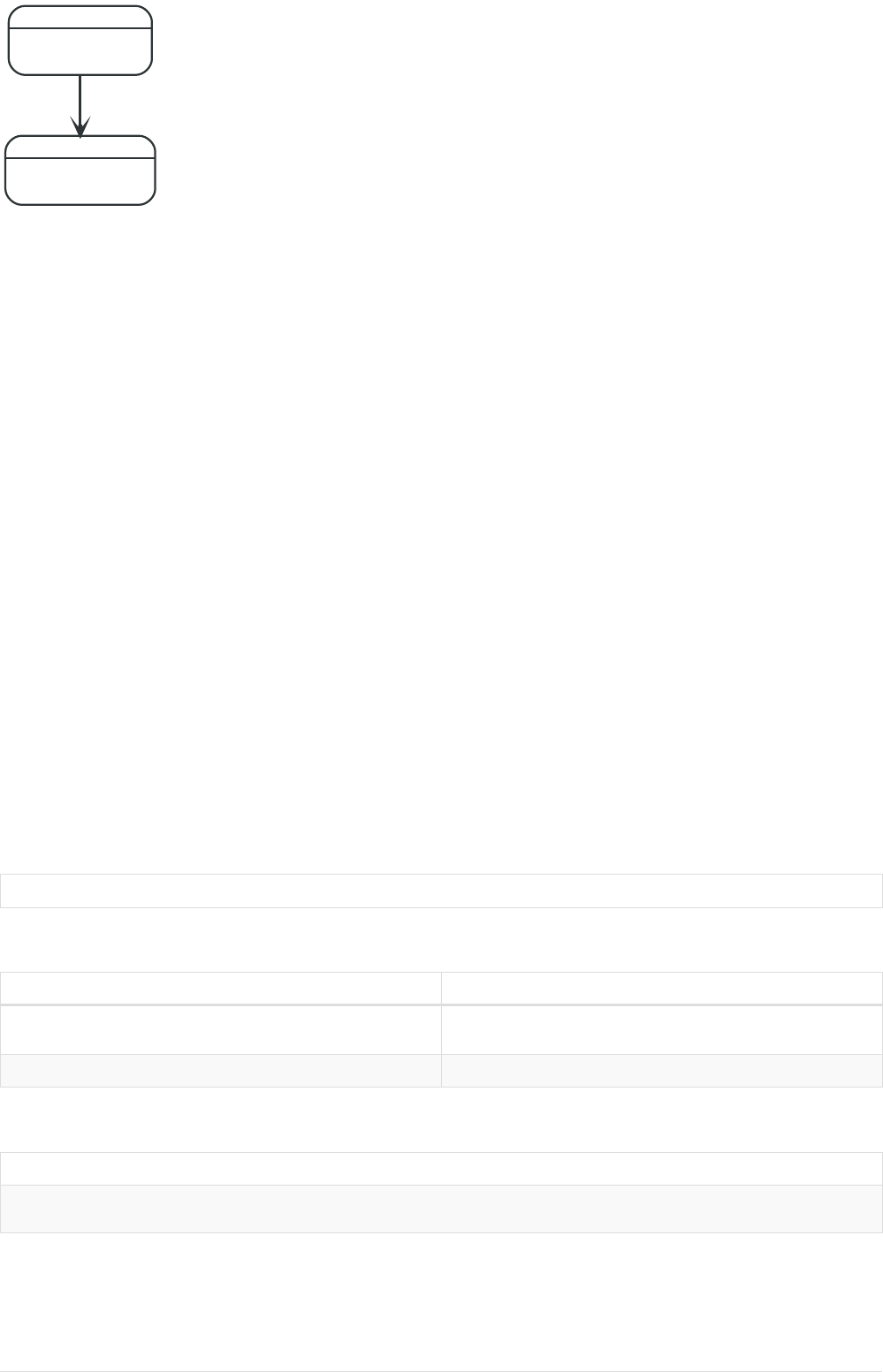
TrainStation
longitude = 12.56459
city = 'Copenhagen'
latitude = 55.672874
Office
longitude = 12.994341
city = 'Malmo'
latitude = 55.611784
TRAVEL_ROUTE
Figure 27. Graph
4.11.1. distance()
distance() returns a floating point number representing the geodesic distance between two points in
the same Coordinate Reference System (CRS).
•If the points are in the Cartesian CRS (2D or 3D), then the units of the returned distance will be the
same as the units of the points, calculated using Pythagoras' theorem.
•If the points are in the WGS-84 CRS (2D), then the units of the returned distance will be meters,
based on the haversine formula over a spherical earth approximation.
•If the points are in the WGS-84 CRS (3D), then the units of the returned distance will be meters.
•The distance is calculated in two steps.
•First, a haversine formula over a spherical earth is used, at the average height of the two
points.
•To account for the difference in height, Pythagoras' theorem is used, combining the
previously calculated spherical distance with the height difference.
•This formula works well for points close to the earth’s surface; for instance, it is well-suited for
calculating the distance of an airplane flight. It is less suitable for greater heights, however,
such as when calculating the distance between two satellites.
Syntax: distance(point1, point2)
Returns:
A Float.
Arguments:
Name Description
point1 A point in either a geographic or cartesian coordinate
system.
point2 A point in the same CRS as 'point1'.
Considerations:
distance(null, null), distance(null, point2) and distance(point1, null) all return null.
Attempting to use points with different Coordinate Reference Systems (such as WGS 84 2D and WGS 84 3D) will return
null.
276

Query
WITH point({ x: 2.3, y: 4.5, crs: 'cartesian' }) AS p1, point({ x: 1.1, y: 5.4, crs: 'cartesian' }) AS p2
RETURN distance(p1,p2) AS dist
The distance between two 2D points in the Cartesian CRS is returned.
Table 376. Result
dist
1.5
1 row
Query
WITH point({ longitude: 12.78, latitude: 56.7, height: 100 }) AS p1, point({ latitude: 56.71, longitude:
12.79, height: 100 }) AS p2
RETURN distance(p1,p2) AS dist
The distance between two 3D points in the WGS 84 CRS is returned.
Table 377. Result
dist
1269.9148706779565
1 row
Query
MATCH (t:TrainStation)-[:TRAVEL_ROUTE]->(o:Office)
WITH point({ longitude: t.longitude, latitude: t.latitude }) AS trainPoint, point({ longitude:
o.longitude, latitude: o.latitude }) AS officePoint
RETURN round(distance(trainPoint, officePoint)) AS travelDistance
The distance between the train station in Copenhagen and the Neo4j office in Malmo is returned.
Table 378. Result
travelDistance
27842.0
1 row
Query
RETURN distance(NULL , point({ longitude: 56.7, latitude: 12.78 })) AS d
If null is provided as one or both of the arguments, null is returned.
Table 379. Result
d
<null>
1 row
277

4.11.2. point() - WGS 84 2D
point({longitude | x, latitude | y [, crs][, srid]}) returns a 2D point in the WGS 84 CRS
corresponding to the given coordinate values.
Syntax: point({longitude | x, latitude | y [, crs][, srid]})
Returns:
A 2D point in WGS 84.
Arguments:
Name Description
A single map consisting of the following:
longitude/x A numeric expression that represents the longitude/x
value in decimal degrees
latitude/y A numeric expression that represents the latitude/y value
in decimal degrees
crs The optional string 'WGS-84'
srid The optional number 4326
Considerations:
If any argument provided to point() is null, null will be returned.
If the coordinates are specified using latitude and longitude, the crs or srid fields are optional and inferred to be
'WGS-84' (srid=4326).
If the coordinates are specified using x and y, then either the crs or srid field is required if a geographic CRS is desired.
Query
RETURN point({ longitude: 56.7, latitude: 12.78 }) AS point
A 2D point with a longitude of 56.7 and a latitude of 12.78 in the WGS 84 CRS is returned.
Table 380. Result
point
point({x: 56.7, y: 12.78, crs: 'wgs-84'})
1 row
Query
RETURN point({ x: 2.3, y: 4.5, crs: 'WGS-84' }) AS point
x and y coordinates may be used in the WGS 84 CRS instead of longitude and latitude, respectively,
providing crs is set to 'WGS-84', or srid is set to 4326.
Table 381. Result
point
point({x: 2.3, y: 4.5, crs: 'wgs-84'})
1 row
278

Query
MATCH (p:Office)
RETURN point({ longitude: p.longitude, latitude: p.latitude }) AS officePoint
A 2D point representing the coordinates of the city of Malmo in the WGS 84 CRS is returned.
Table 382. Result
officePoint
point({x: 12.994341, y: 55.611784, crs: 'wgs-84'})
1 row
Query
RETURN point(NULL ) AS p
If null is provided as the argument, null is returned.
Table 383. Result
p
<null>
1 row
4.11.3. point() - WGS 84 3D
point({longitude | x, latitude | y, height | z, [, crs][, srid]}) returns a 3D point in the WGS
84 CRS corresponding to the given coordinate values.
Syntax: point({longitude | x, latitude | y, height | z, [, crs][, srid]})
Returns:
A 3D point in WGS 84.
Arguments:
Name Description
A single map consisting of the following:
longitude/x A numeric expression that represents the longitude/x
value in decimal degrees
latitude/y A numeric expression that represents the latitude/y value
in decimal degrees
height/z A numeric expression that represents the height/z value in
meters
crs The optional string 'WGS-84-3D'
srid The optional number 4979
Considerations:
If any argument provided to point() is null, null will be returned.
If the height/z key and value is not provided, a 2D point in the WGS 84 CRS will be returned.
279

If the coordinates are specified using latitude and longitude, the crs or srid fields are optional and inferred to be
'WGS-84-3D' (srid=4979).
If the coordinates are specified using x and y, then either the crs or srid field is required if a geographic CRS is desired.
Query
RETURN point({ longitude: 56.7, latitude: 12.78, height: 8 }) AS point
A 3D point with a longitude of 56.7, a latitude of 12.78 and a height of 8 meters in the WGS 84 CRS is
returned.
Table 384. Result
point
point({x: 56.7, y: 12.78, z: 8.0, crs: 'wgs-84-3d'})
1 row
4.11.4. point() - Cartesian 2D
point({x, y [, crs][, srid]}) returns a 2D point in the Cartesian CRS corresponding to the given
coordinate values.
Syntax: point({x, y [, crs][, srid]})
Returns:
A 2D point in Cartesian.
Arguments:
Name Description
A single map consisting of the following:
xA numeric expression
yA numeric expression
crs The optional string 'cartesian'
srid The optional number 7203
Considerations:
If any argument provided to point() is null, null will be returned.
The crs or srid fields are optional and default to the Cartesian CRS (which means srid:7203).
Query
RETURN point({ x: 2.3, y: 4.5 }) AS point
A 2D point with an x coordinate of 2.3 and a y coordinate of 4.5 in the Cartesian CRS is returned.
Table 385. Result
point
point({x: 2.3, y: 4.5, crs: 'cartesian'})
280

point
1 row
4.11.5. point() - Cartesian 3D
point({x, y, z, [, crs][, srid]}) returns a 3D point in the Cartesian CRS corresponding to the given
coordinate values.
Syntax: point({x, y, z, [, crs][, srid]})
Returns:
A 3D point in Cartesian.
Arguments:
Name Description
A single map consisting of the following:
xA numeric expression
yA numeric expression
zA numeric expression
crs The optional string 'cartesian-3D'
srid The optional number 9157
Considerations:
If any argument provided to point() is null, null will be returned.
If the z key and value is not provided, a 2D point in the Cartesian CRS will be returned.
The crs or srid fields are optional and default to the 3D Cartesian CRS (which means srid:9157).
Query
RETURN point({ x: 2.3, y: 4.5, z: 2 }) AS point
A 3D point with an x coordinate of 2.3, a y coordinate of 4.5 and a z coordinate of 2 in the Cartesian
CRS is returned.
Table 386. Result
point
point({x: 2.3, y: 4.5, z: 2.0, crs: 'cartesian-3d'})
1 row
4.12. User-defined functions
User-defined functions are written in Java, deployed into the database and are called in the same way
as any other Cypher function.
This example shows how you invoke a user-defined function called join from Cypher.
281

4.12.1. Call a user-defined function
This calls the user-defined function org.neo4j.procedure.example.join().
Query
MATCH (n:Member)
RETURN org.neo4j.function.example.join(collect(n.name)) AS members
Table 387. Result
members
"John,Paul,George,Ringo"
1 row
For developing and deploying user-defined functions in Neo4j, see Extending Neo4j → User-defined
functions.
4.12.2. User-defined aggregation functions
User-defined aggregation functions are written in Java, deployed into the database and are called in
the same way as any other Cypher function.
This example shows how you invoke a user-defined aggregation function called longestString from
Cypher.
4.13. User-defined aggregation functions
User-defined aggregation functions are written in Java, deployed into the database and are
called in the same way as any other Cypher function.
This example shows how you invoke a user-defined aggregation function called longestString from
Cypher.
4.13.1. Call a user-defined aggregation function
This calls the user-defined function org.neo4j.function.example.longestString().
Query
MATCH (n:Member)
RETURN org.neo4j.function.example.longestString(n.name) AS member
Table 388. Result
member
"George"
1 row
For developing and deploying user-defined aggregation functions in Neo4j, see Extending Neo4j →
User-defined aggregation functions.
282

Chapter 5. Schema
This section explains how to work with an optional schema in Neo4j in the Cypher query
language.
Labels are used in the specification of indexes, and for defining constraints on the graph. Together,
indexes and constraints are the schema of the graph. Cypher includes data definition language (DDL)
statements for manipulating the schema.
•Indexes
•Create a single-property index
•Create a composite index
•Get a list of all indexes in the database
•Drop a single-property index
•Drop a composite index
•Use index
•Equality check using WHERE (single-property index)
•Equality check using WHERE (composite index)
•Range comparisons using WHERE (single-property index)
•Use index with WHERE using multiple range comparisons
•List membership using IN (single-property index)
•List membership check using IN (composite index)
•Prefix search using STARTS WITH (single-property index)
•Suffix search using ENDS WITH (single-property index)
•Substring search using CONTAINS (single-property index)
•Existence check using exists (single-property index)
•Use index when executing a spatial distance search
•Use index when executing a spatial bounding box search
•Fulltext schema index
•Introduction
•Create and configure fulltext schema indexes
•Query fulltext schema indexes
•Manage and use explicit indexes
•Constraints
•Unique node property constraints
•Get a list of all constraints in the database
•Node property existence constraints
•Relationship property existence constraints
•Node Keys
283

5.1. Indexes
This section explains how to work with indexes in Neo4j and Cypher.
•Introduction
•Create a single-property index
•Create a composite index
•Get a list of all indexes in the database
•Drop a single-property index
•Drop a composite index
•Use index
•Equality check using WHERE (single-property index)
•Equality check using WHERE (composite index)
•Range comparisons using WHERE (single-property index)
•Use index with WHERE using multiple range comparisons
•List membership check using IN (single-property index)
•List membership check using IN (composite index)
•Prefix search using STARTS WITH (single-property index)
•Suffix search using ENDS WITH (single-property index)
•Substring search using CONTAINS (single-property index)
•Existence check using exists (single-property index)
•Use index when executing a spatial distance search
•Use index when executing a spatial bounding box search
•Fulltext schema index
•Introduction
•Create and configure fulltext schema indexes
•Query fulltext schema indexes
•Manage and use explicit indexes
5.1.1. Introduction
A database index is a redundant copy of some of the data in the database for the purpose of making
searches of related data more efficient. This comes at the cost of additional storage space and slower
writes, so deciding what to index and what not to index is an important and often non-trivial task.
Cypher enables the creation of indexes on one or more properties for all nodes that have a given
label:
•An index that is created on a single property for any given label is called a single-property index.
•An index that is created on more than one property for any given label is called a composite index.
Differences in the usage patterns between composite and single-property indexes are detailed in
the examples below.
Once an index has been created, it will automatically be managed and kept up to date by the database
284

when the graph is changed. Neo4j will automatically pick up and start using the index once it has been
created and brought online.
Planner hints and the USING keyword describes how to make the Cypher planner
use specific indexes (especially in cases where the planner would not necessarily
have used them).
Index configuration and limitations
For information on index configuration and limitations, refer to Operations Manual
→ Index configuration.
5.1.2. Create a single-property index
An index on a single property for all nodes that have a particular label can be created with CREATE
INDEX ON :Label(property). Note that the index is not immediately available, but will be created in the
background.
Query
CREATE INDEX ON :Person(firstname)
Result
+--------------------------------------------+
| No data returned, and nothing was changed. |
+--------------------------------------------+
5.1.3. Create a composite index
An index on multiple properties for all nodes that have a particular label — i.e. a composite
index — can be created with CREATE INDEX ON :Label(prop1, …, propN). Only nodes labeled with the
specified label and which contain all the properties in the index definition will be added to the index.
The following statement will create a composite index on all nodes labeled with Person and which
have both an age and country property:
Query
CREATE INDEX ON :Person(age, country)
Assume we execute the query CREATE (a:Person {firstname: 'Bill', age: 34, country: 'USA'}),
(b:Person {firstname: 'Sue', age: 39}). Node a has both an age and a country property, and so it will
be added to the composite index. However, as node b has no country property, it will not be added to
the composite index. Note that the composite index is not immediately available, but will be created in
the background.
Result
+-------------------+
| No data returned. |
+-------------------+
Indexes added: 1
5.1.4. Get a list of all indexes in the database
Calling the built-in procedure db.indexes will list all the indexes in the database.
285

Query
CALL db.indexes
Result
+---------------------------------------------------------------------------------------------------------
-------------------------------------------------------------------------------------+
| description | indexName | tokenNames | properties | state | type
| progress | provider | id | failureMessage |
+---------------------------------------------------------------------------------------------------------
-------------------------------------------------------------------------------------+
| "INDEX ON :Person(firstname)" | "Unnamed index" | ["Person"] | ["firstname"] | "ONLINE" |
"node_label_property" | 100.0 | {version -> "1.0", key -> "native-btree"} | 3 | "" |
| "INDEX ON :Person(highScore)" | "Unnamed index" | ["Person"] | ["highScore"] | "ONLINE" |
"node_label_property" | 100.0 | {version -> "1.0", key -> "native-btree"} | 1 | "" |
| "INDEX ON :Person(location)" | "Unnamed index" | ["Person"] | ["location"] | "ONLINE" |
"node_label_property" | 100.0 | {version -> "1.0", key -> "native-btree"} | 5 | "" |
+---------------------------------------------------------------------------------------------------------
-------------------------------------------------------------------------------------+
3 rows
5.1.5. Drop a single-property index
An index on all nodes that have a label and single property combination can be dropped with DROP
INDEX ON :Label(property).
Query
DROP INDEX ON :Person(firstname)
Result
+-------------------+
| No data returned. |
+-------------------+
Indexes removed: 1
5.1.6. Drop a composite index
A composite index on all nodes that have a label and multiple property combination can be dropped
with DROP INDEX ON :Label(prop1, …, propN). The following statement will drop a composite index on
all nodes labeled with Person and which have both an age and country property:
Query
DROP INDEX ON :Person(age, country)
Result
+-------------------+
| No data returned. |
+-------------------+
Indexes removed: 1
5.1.7. Use index
There is usually no need to specify which indexes to use in a query, Cypher will figure that out by itself.
For example the query below will use the Person(firstname) index, if it exists.
286

Query
MATCH (person:Person { firstname: 'Andy' })
RETURN person
Query Plan
Compiler CYPHER 3.5
Planner COST
Runtime INTERPRETED
Runtime version 3.5
+-----------------+----------------+------+---------+-----------------+-------------------
+----------------------+----------------------+-----------+--------------------+
| Operator | Estimated Rows | Rows | DB Hits | Page Cache Hits | Page Cache Misses | Page Cache Hit
Ratio | Order | Variables | Other |
+-----------------+----------------+------+---------+-----------------+-------------------
+----------------------+----------------------+-----------+--------------------+
| +ProduceResults | 1 | 1 | 0 | 2 | 1 |
0.6667 | person.firstname ASC | person | |
| | +----------------+------+---------+-----------------+-------------------
+----------------------+----------------------+-----------+--------------------+
| +NodeIndexSeek | 1 | 1 | 3 | 2 | 1 |
0.6667 | person.firstname ASC | person | :Person(firstname) |
+-----------------+----------------+------+---------+-----------------+-------------------
+----------------------+----------------------+-----------+--------------------+
Total database accesses: 3
5.1.8. Equality check using WHERE (single-property index)
A query containing equality comparisons of a single indexed property in the WHERE clause is backed
automatically by the index. It is also possible for a query with multiple OR predicates to use multiple
indexes, if indexes exist on the properties. For example, if indexes exist on both :Label(p1) and
:Label(p2), MATCH (n:Label) WHERE n.p1 = 1 OR n.p2 = 2 RETURN n will use both indexes.
Query
MATCH (person:Person)
WHERE person.firstname = 'Andy'
RETURN person
287

Query Plan
Compiler CYPHER 3.5
Planner COST
Runtime INTERPRETED
Runtime version 3.5
+-----------------+----------------+------+---------+-----------------+-------------------
+----------------------+----------------------+-----------+--------------------+
| Operator | Estimated Rows | Rows | DB Hits | Page Cache Hits | Page Cache Misses | Page Cache Hit
Ratio | Order | Variables | Other |
+-----------------+----------------+------+---------+-----------------+-------------------
+----------------------+----------------------+-----------+--------------------+
| +ProduceResults | 1 | 1 | 0 | 2 | 1 |
0.6667 | person.firstname ASC | person | |
| | +----------------+------+---------+-----------------+-------------------
+----------------------+----------------------+-----------+--------------------+
| +NodeIndexSeek | 1 | 1 | 3 | 2 | 1 |
0.6667 | person.firstname ASC | person | :Person(firstname) |
+-----------------+----------------+------+---------+-----------------+-------------------
+----------------------+----------------------+-----------+--------------------+
Total database accesses: 3
5.1.9. Equality check using WHERE (composite index)
A query containing equality comparisons for all the properties of a composite index will automatically
be backed by the same index. The following query will use the composite index defined earlier:
Query
MATCH (n:Person)
WHERE n.age = 35 AND n.country = 'UK'
RETURN n
However, the query MATCH (n:Person) WHERE n.age = 35 RETURN n will not be backed by the composite
index, as the query does not contain an equality predicate on the country property. It will only be
backed by an index on the Person label and age property defined thus: :Person(age); i.e. a single-
property index. Moreover, unlike single-property indexes, composite indexes currently do not support
queries containing the following types of predicates on properties in the index: existence check:
exists(n.prop); range search: n.prop > value; prefix search: STARTS WITH; suffix search: ENDS WITH; and
substring search: CONTAINS.
Result
+-------------------------------------------------------------------------------------------+
| n |
+-------------------------------------------------------------------------------------------+
| Node[0]{country:"UK",highScore:54321,firstname:"John",surname:"Smith",name:"john",age:35} |
+-------------------------------------------------------------------------------------------+
1 row
5.1.10. Range comparisons using WHERE (single-property index)
Single-property indexes are also automatically used for inequality (range) comparisons of an indexed
property in the WHERE clause. Composite indexes are currently not able to support range comparisons.
288

Query
MATCH (person:Person)
WHERE person.firstname > 'B'
RETURN person
Query Plan
Compiler CYPHER 3.5
Planner COST
Runtime INTERPRETED
Runtime version 3.5
+-----------------------+----------------+------+---------+-----------------+-------------------
+----------------------+----------------------+-----------+--------------------------------------+
| Operator | Estimated Rows | Rows | DB Hits | Page Cache Hits | Page Cache Misses | Page
Cache Hit Ratio | Order | Variables | Other |
+-----------------------+----------------+------+---------+-----------------+-------------------
+----------------------+----------------------+-----------+--------------------------------------+
| +ProduceResults | 0 | 1 | 0 | 2 | 1 |
0.6667 | person.firstname ASC | person | |
| | +----------------+------+---------+-----------------+-------------------
+----------------------+----------------------+-----------+--------------------------------------+
| +NodeIndexSeekByRange | 0 | 1 | 3 | 2 | 1 |
0.6667 | person.firstname ASC | person | :Person(firstname) > { AUTOSTRING0} |
+-----------------------+----------------+------+---------+-----------------+-------------------
+----------------------+----------------------+-----------+--------------------------------------+
Total database accesses: 3
5.1.11. Multiple range comparisons using WHERE (single-property
index)
When the WHERE clause contains multiple inequality (range) comparisons for the same property, these
can be combined in a single index range seek.
Query
MATCH (person:Person)
WHERE 10000 < person.highScore < 20000
RETURN person
289

Query Plan
Compiler CYPHER 3.5
Planner COST
Runtime INTERPRETED
Runtime version 3.5
+-----------------------+----------------+------+---------+-----------------+-------------------
+----------------------+----------------------+-----------
+-------------------------------------------------------------------------+
| Operator | Estimated Rows | Rows | DB Hits | Page Cache Hits | Page Cache Misses | Page
Cache Hit Ratio | Order | Variables | Other
|
+-----------------------+----------------+------+---------+-----------------+-------------------
+----------------------+----------------------+-----------
+-------------------------------------------------------------------------+
| +ProduceResults | 0 | 1 | 0 | 2 | 1 |
0.6667 | person.highScore ASC | person |
|
| | +----------------+------+---------+-----------------+-------------------
+----------------------+----------------------+-----------
+-------------------------------------------------------------------------+
| +NodeIndexSeekByRange | 0 | 1 | 3 | 2 | 1 |
0.6667 | person.highScore ASC | person | :Person(highScore) > { AUTOINT1} AND :Person(highScore) < {
AUTOINT0} |
+-----------------------+----------------+------+---------+-----------------+-------------------
+----------------------+----------------------+-----------
+-------------------------------------------------------------------------+
Total database accesses: 3
5.1.12. List membership check using IN (single-property index)
The IN predicate on person.firstname in the following query will use the single-property index
Person(firstname) if it exists.
Query
MATCH (person:Person)
WHERE person.firstname IN ['Andy', 'John']
RETURN person
Query Plan
Compiler CYPHER 3.5
Planner COST
Runtime INTERPRETED
Runtime version 3.5
+-----------------+----------------+------+---------+-----------------+-------------------
+----------------------+-----------+--------------------+
| Operator | Estimated Rows | Rows | DB Hits | Page Cache Hits | Page Cache Misses | Page Cache Hit
Ratio | Variables | Other |
+-----------------+----------------+------+---------+-----------------+-------------------
+----------------------+-----------+--------------------+
| +ProduceResults | 24 | 2 | 0 | 4 | 2 |
0.6667 | person | |
| | +----------------+------+---------+-----------------+-------------------
+----------------------+-----------+--------------------+
| +NodeIndexSeek | 24 | 2 | 5 | 4 | 2 |
0.6667 | person | :Person(firstname) |
+-----------------+----------------+------+---------+-----------------+-------------------
+----------------------+-----------+--------------------+
Total database accesses: 5
290

5.1.13. List membership check using IN (composite index)
The IN predicates on person.age and person.country in the following query will use the composite
index Person(age, country) if it exists.
Query
MATCH (person:Person)
WHERE person.age IN [10, 20, 35] AND person.country IN ['Sweden', 'USA', 'UK']
RETURN person
Query Plan
Compiler CYPHER 3.5
Planner COST
Runtime INTERPRETED
Runtime version 3.5
+-----------------+----------------+------+---------+-----------------+-------------------
+----------------------+-----------+----------------------+
| Operator | Estimated Rows | Rows | DB Hits | Page Cache Hits | Page Cache Misses | Page Cache Hit
Ratio | Variables | Other |
+-----------------+----------------+------+---------+-----------------+-------------------
+----------------------+-----------+----------------------+
| +ProduceResults | 451 | 1 | 0 | 18 | 2 |
0.9000 | person | |
| | +----------------+------+---------+-----------------+-------------------
+----------------------+-----------+----------------------+
| +NodeIndexSeek | 451 | 1 | 11 | 18 | 2 |
0.9000 | person | :Person(age,country) |
+-----------------+----------------+------+---------+-----------------+-------------------
+----------------------+-----------+----------------------+
Total database accesses: 11
5.1.14. Prefix search using STARTS WITH (single-property index)
The STARTS WITH predicate on person.firstname in the following query will use the Person(firstname)
index, if it exists. Composite indexes are currently not able to support STARTS WITH.
Query
MATCH (person:Person)
WHERE person.firstname STARTS WITH 'And'
RETURN person
291

Query Plan
Compiler CYPHER 3.5
Planner COST
Runtime INTERPRETED
Runtime version 3.5
+-----------------------+----------------+------+---------+-----------------+-------------------
+----------------------+----------------------+-----------
+-------------------------------------------------+
| Operator | Estimated Rows | Rows | DB Hits | Page Cache Hits | Page Cache Misses | Page
Cache Hit Ratio | Order | Variables | Other |
+-----------------------+----------------+------+---------+-----------------+-------------------
+----------------------+----------------------+-----------
+-------------------------------------------------+
| +ProduceResults | 2 | 1 | 0 | 3 | 0 |
1.0000 | person.firstname ASC | person | |
| | +----------------+------+---------+-----------------+-------------------
+----------------------+----------------------+-----------
+-------------------------------------------------+
| +NodeIndexSeekByRange | 2 | 1 | 3 | 3 | 0 |
1.0000 | person.firstname ASC | person | :Person(firstname STARTS WITH $` AUTOSTRING0`) |
+-----------------------+----------------+------+---------+-----------------+-------------------
+----------------------+----------------------+-----------
+-------------------------------------------------+
Total database accesses: 3
5.1.15. Suffix search using ENDS WITH (single-property index)
The ENDS WITH predicate on person.firstname in the following query will use the Person(firstname)
index, if it exists. All values stored in the Person(firstname) index will be searched, and entries ending
with 'hn' will be returned. This means that although the search will not be optimized to the extent of
queries using =, IN, >, < or STARTS WITH, it is still faster than not using an index in the first place.
Composite indexes are currently not able to support ENDS WITH.
Query
MATCH (person:Person)
WHERE person.firstname ENDS WITH 'hn'
RETURN person
292

Query Plan
Compiler CYPHER 3.5
Planner COST
Runtime INTERPRETED
Runtime version 3.5
+------------------------+----------------+------+---------+-----------------+-------------------
+----------------------+----------------------+-----------+--------------------------------------+
| Operator | Estimated Rows | Rows | DB Hits | Page Cache Hits | Page Cache Misses | Page
Cache Hit Ratio | Order | Variables | Other |
+------------------------+----------------+------+---------+-----------------+-------------------
+----------------------+----------------------+-----------+--------------------------------------+
| +ProduceResults | 2 | 1 | 0 | 2 | 0 |
1.0000 | person.firstname ASC | person | |
| | +----------------+------+---------+-----------------+-------------------
+----------------------+----------------------+-----------+--------------------------------------+
| +NodeIndexEndsWithScan | 2 | 1 | 3 | 3 | 0 |
1.0000 | person.firstname ASC | person | :Person(firstname); $` AUTOSTRING0` |
+------------------------+----------------+------+---------+-----------------+-------------------
+----------------------+----------------------+-----------+--------------------------------------+
Total database accesses: 3
5.1.16. Substring search using CONTAINS (single-property index)
The CONTAINS predicate on person.firstname in the following query will use the Person(firstname)
index, if it exists. All values stored in the Person(firstname) index will be searched, and entries
containing 'h' will be returned. This means that although the search will not be optimized to the
extent of queries using =, IN, >, < or STARTS WITH, it is still faster than not using an index in the first
place. Composite indexes are currently not able to support CONTAINS.
Query
MATCH (person:Person)
WHERE person.firstname CONTAINS 'h'
RETURN person
Query Plan
Compiler CYPHER 3.5
Planner COST
Runtime INTERPRETED
Runtime version 3.5
+------------------------+----------------+------+---------+-----------------+-------------------
+----------------------+----------------------+-----------+--------------------------------------+
| Operator | Estimated Rows | Rows | DB Hits | Page Cache Hits | Page Cache Misses | Page
Cache Hit Ratio | Order | Variables | Other |
+------------------------+----------------+------+---------+-----------------+-------------------
+----------------------+----------------------+-----------+--------------------------------------+
| +ProduceResults | 2 | 1 | 0 | 2 | 0 |
1.0000 | person.firstname ASC | person | |
| | +----------------+------+---------+-----------------+-------------------
+----------------------+----------------------+-----------+--------------------------------------+
| +NodeIndexContainsScan | 2 | 1 | 3 | 3 | 0 |
1.0000 | person.firstname ASC | person | :Person(firstname); $` AUTOSTRING0` |
+------------------------+----------------+------+---------+-----------------+-------------------
+----------------------+----------------------+-----------+--------------------------------------+
Total database accesses: 3
293

5.1.17. Existence check using exists (single-property index)
The exists(p.firstname) predicate in the following query will use the Person(firstname) index, if it
exists. Composite indexes are currently not able to support the exists predicate.
Query
MATCH (p:Person)
WHERE exists(p.firstname)
RETURN p
Query Plan
Compiler CYPHER 3.5
Planner COST
Runtime INTERPRETED
Runtime version 3.5
+-----------------+----------------+------+---------+-----------------+-------------------
+----------------------+-----------+--------------------+
| Operator | Estimated Rows | Rows | DB Hits | Page Cache Hits | Page Cache Misses | Page Cache Hit
Ratio | Variables | Other |
+-----------------+----------------+------+---------+-----------------+-------------------
+----------------------+-----------+--------------------+
| +ProduceResults | 2 | 2 | 0 | 2 | 0 |
1.0000 | p | |
| | +----------------+------+---------+-----------------+-------------------
+----------------------+-----------+--------------------+
| +NodeIndexScan | 2 | 2 | 4 | 2 | 1 |
0.6667 | p | :Person(firstname) |
+-----------------+----------------+------+---------+-----------------+-------------------
+----------------------+-----------+--------------------+
Total database accesses: 4
5.1.18. Spatial distance searches (single-property index)
If a property with point values is indexed, the index is used for spatial distance searches as well as for
range queries.
Query
MATCH (p:Person)
WHERE distance(p.location, point({ x: 1, y: 2 }))< 2
RETURN p.location
294

Query Plan
Compiler CYPHER 3.5
Planner COST
Runtime INTERPRETED
Runtime version 3.5
+-----------------------+----------------+------+---------+-----------------+-------------------
+----------------------+-----------------------
+-------------------------------------------------------------------------------------------+
| Operator | Estimated Rows | Rows | DB Hits | Page Cache Hits | Page Cache Misses | Page
Cache Hit Ratio | Variables | Other
|
+-----------------------+----------------+------+---------+-----------------+-------------------
+----------------------+-----------------------
+-------------------------------------------------------------------------------------------+
| +ProduceResults | 0 | 9 | 0 | 6 | 0 |
1.0000 | p, p.location |
|
| | +----------------+------+---------+-----------------+-------------------
+----------------------+-----------------------
+-------------------------------------------------------------------------------------------+
| +Projection | 0 | 9 | 0 | 6 | 0 |
1.0000 | p.location -- p | {p.location : cached[p.location]}
|
| | +----------------+------+---------+-----------------+-------------------
+----------------------+-----------------------
+-------------------------------------------------------------------------------------------+
| +Filter | 0 | 9 | 0 | 6 | 0 |
1.0000 | cached[p.location], p | distance(cached[p.location], point({x: $` AUTOINT0`, y: $` AUTOINT1`}))
< $` AUTOINT2` |
| | +----------------+------+---------+-----------------+-------------------
+----------------------+-----------------------
+-------------------------------------------------------------------------------------------+
| +NodeIndexSeekByRange | 0 | 9 | 11 | 6 | 0 |
1.0000 | cached[p.location], p | :Person(location) WHERE distance(_,point(x,y)) < Parameter(
AUTOINT2,Integer) |
+-----------------------+----------------+------+---------+-----------------+-------------------
+----------------------+-----------------------
+-------------------------------------------------------------------------------------------+
Total database accesses: 11
5.1.19. Spatial bounding box searches (single-property index)
The ability to do index seeks on bounded ranges works even with the 2D and 3D spatial Point types.
Query
MATCH (person:Person)
WHERE point({ x: 1, y: 5 })< person.location < point({ x: 2, y: 6 })
RETURN person
295

Query Plan
Compiler CYPHER 3.5
Planner COST
Runtime INTERPRETED
Runtime version 3.5
+-----------------------+----------------+------+---------+-----------------+-------------------
+----------------------+-----------
+---------------------------------------------------------------------------------------------------------
------------------------+
| Operator | Estimated Rows | Rows | DB Hits | Page Cache Hits | Page Cache Misses | Page
Cache Hit Ratio | Variables | Other
|
+-----------------------+----------------+------+---------+-----------------+-------------------
+----------------------+-----------
+---------------------------------------------------------------------------------------------------------
------------------------+
| +ProduceResults | 0 | 1 | 0 | 8 | 0 |
1.0000 | person |
|
| | +----------------+------+---------+-----------------+-------------------
+----------------------+-----------
+---------------------------------------------------------------------------------------------------------
------------------------+
| +NodeIndexSeekByRange | 0 | 1 | 3 | 8 | 0 |
1.0000 | person | :Person(location) > point({x: { AUTOINT2}, y: { AUTOINT3}}) AND :Person(location) <
point({x: { AUTOINT0}, y: { AUTOINT1}}) |
+-----------------------+----------------+------+---------+-----------------+-------------------
+----------------------+-----------
+---------------------------------------------------------------------------------------------------------
------------------------+
Total database accesses: 3
5.1.20. Fulltext schema index
The fulltext schema indexes can be used to index nodes and relationships by string
properties, and query by either exact or fuzzy matching.
Introduction
Fulltext schema indexes are powered by the Apache Lucene (http://lucene.apache.org/) indexing and
search library. A fulltext schema index allows you to write queries that matches within the contents of
indexed string properties. For instance, the regular schema indexes described in previous sections can
only do exact matching or prefix matches on strings. A fulltext index will instead tokenize the indexed
string values, so it can match terms anywhere within the strings. How the indexed strings are
tokenized and broken into terms, is determined by what analyzer the fulltext schema index is
configured with. For instance, the swedish analyzer knows how to tokenize and stem Swedish words,
and will avoid indexing Swedish stop words.
Fulltext schema indexes:
•support the indexing of both nodes and relationships.
•support configuring custom analyzers, including analyzers that are not included with Lucene itself.
•can be queried using the Lucene query language.
•can return the score for each result from a query.
•are kept up to date automatically, as nodes and relationships are added, removed, and modified.
•will automatically populate newly created indexes with the existing data in a store.
296

•can be checked by the consistency checker, and they can be rebuilt if there is a problem with
them.
•are a projection of the store, and can only index nodes and relationships by the contents of their
properties.
•can support any number of documents in a single index.
•are created, dropped, and updated transactionally, and is automatically replicated throughout a
cluster.
•can be accessed via Cypher procedures.
•can be configured to be eventually consistent, in which index updating is moved from the commit
path to a background thread. Using this feature, it is possible to work around the slow Lucene
writes from the performance critical commit process, thus removing the main bottlenecks for
Neo4j write performance.
For information on how to configure fulltext schema indexes, refer to Operations Manual → Fulltext
schema indexes.
Fulltext schema indexes replace the explicit indexes, which are deprecated and will
be discontinued in the next major release. It is therefore recommended migrate to
fulltext schema indexes. A full description of the differences between fulltext
schema indexes and explicit indexes is available in Operations Manual →
Deprecation of explicit indexes.
Create and configure fulltext schema indexes
Fulltext schema indexes are created with the db.index.fulltext.createNodeIndex and
db.index.fulltext.createRelationshipIndex. The indexes must each be given a unique name when
created, which is used to reference the specific index in question, when querying or dropping an
index. A fulltext schema index then applies to a list of labels or a list of relationship types, for node
and relationship indexes respectively, and then a list of property names.
An index that applies to more than one label, or more than one relationship type, is called a multi-
token index. Multi-token indexes can also apply to more than one property at a time, like a composite
index can, but with an important difference. A composite index applies only to entities that match the
indexed label and all of the indexed properties. A multi-token index, on the other hand, will index
entities that have at least one of the indexed labels or relationship types, and any of the indexed
properties.
For instance, if we have a movie with a title.
Query
CREATE (m:Movie { title: "The Matrix" })
RETURN m.title
Table 389. Result
m.title
"The Matrix"
1 row
Nodes created: 1
Properties set: 1
Labels added: 1
And we have a fulltext schema index on the title and description properties of movies and books.
297

Query
CALL db.index.fulltext.createNodeIndex("titlesAndDescriptions",["Movie", "Book"],["title", "description"])
Then our movie node from above will be included in the index, even though it only have one of the
indexed labels, and only one of the indexed properties:
Query
CALL db.index.fulltext.queryNodes("titlesAndDescriptions", "matrix") YIELD node, score
RETURN node.title, node.description, score
Table 390. Result
node.title node.description score
"The Matrix" <null> 1.261009693145752
1 row
The same is true for fulltext schema indexes on relationships. Though a relationship can only have
one type, a relationship fulltext schema index can index multiple types, and all relationships will be
included that match one of the relationship types, and at least one of the indexed properties.
The db.index.fulltext.createNodeIndex and db.index.fulltext.createRelationshipIndex takes an
optional fourth argument, called config. The config parameter is a map from string to string, and can
be used to set index-specific configuration settings. The analyzer setting can be used to configure an
index-specific analyzer. The possible values for the analyzer setting can be listed with the
db.index.fulltext.listAvailableAnalyzers procedure. The eventually_consistent setting, if set to
"true", will put the index in an eventually consistent update mode. this means that updates will be
applied in a background thread "as soon as possible", instead of during transaction commit like other
indexes.
Using index-specific settings via the config parameter is experimental, because
these settings currently do not get replicated in a clustered environment. See the
Fulltext Schema Indexes section of the Operations Manual, for how to configure the
default fulltext index configurations in neo4j.conf.
Query
CALL db.index.fulltext.createRelationshipIndex("taggedByRelationshipIndex",["TAGGED_AS"],["taggedByUser"],
{ analyzer: "url_or_email", eventually_consistent: "true" })
In this example, an eventually consistent relationship fulltext schema index is created for the
TAGGED_AS relationship type, and the taggedByUser property, and the index uses the url_or_email
analyzer. This could, for instance, be a system where people are assigning tags to documents, and
where the index on the taggedByUser property will allow them to quickly find all of the documents they
have tagged. Had it not been for the relationship index, one would have had to add artificial
connective nodes between the tags and the documents in the data model, just so these nodes could
be indexed.
Table 391. Result
(empty result)
0 rows
298

Query fulltext schema indexes
Fulltext indexes will, in addition to any exact matches, also return approximate matches to a given
query. Both the property values that are indexed, and the queries to the index, are processed through
the analyzer such that the index can find that don’t exactly matches. The score that is returned
alongside each result entry, represents how well the index thinks that entry matches the given query.
The results are always returned in descending score order, where the best matching result entry is put
first. To illustrate, in the example below, we search our movie database for "Full Metal Jacket", and
even though there is an exact match as the first result, we also get three other less interesting results:
Query
CALL db.index.fulltext.queryNodes("titlesAndDescriptions", "Full Metal Jacket") YIELD node, score
RETURN node.title, score
Table 392. Result
node.title score
"Full Metal Jacket" 0.8093575239181519
"The Jacket" 0.1152719184756279
"Full Moon High" 0.0836455449461937
"Yellow Jacket" 0.07204495370388031
4 rows
The fulltext schema indexes uses Lucene under the hood. This means that we can use Lucene’s fulltext
query language to express what we wish to search for. For instance, if we are only interested in exact
matches, then we can quote the string we are searching for.
Query
CALL db.index.fulltext.queryNodes("titlesAndDescriptions", "\"Full Metal Jacket\"") YIELD node, score
RETURN node.title, score
When we put "Full Metal Jacket" in quotes, Lucene only gives us exact matches.
Table 393. Result
node.title score
"Full Metal Jacket" 1.3701786994934082
1 row
Lucene also allows us to use logical operators, such as AND and OR, to search for terms:
Query
CALL db.index.fulltext.queryNodes("titlesAndDescriptions", 'full AND metal') YIELD node, score
RETURN node.title, score
Only the "Full Metal Jacket" movie in our database has both the words "full" and "metal".
Table 394. Result
node.title score
"Full Metal Jacket" 0.7603841423988342
1 row
299

It is also possible to search for only specific properties, by putting the property name and a colon in
front of the text being searched for.
Query
CALL db.index.fulltext.queryNodes("titlesAndDescriptions", 'description:"surreal adventure"') YIELD node,
score
RETURN node.title, node.description, score
Table 395. Result
node.title node.description score
"Metallica Through The Never" "The movie follows the young roadie
Trip through his surreal adventure
with the band."
1.311632513999939
1 row
A complete description of the Lucene query syntax can be found in the Lucene documentation
(http://lucene.apache.org/core/5_5_0/queryparser/org/apache/lucene/queryparser/classic/package-
summary.html#package.description).
5.1.21. Manage and use explicit indexes
Explicit indexes are alternative data structures, in which a user can explicitly maintain search and seek
data for nodes and relationships. These data structures are special-purpose and the procedures are
primarily provided for users who have legacy deployments depending on such structures.
The explicit indexing features in Neo4j are deprecated for removal in the next major
release. Consider using schema indexes, or the fulltext schema indexes, instead.
Signature Description
db.index.explicit.addNode Add a node to an explicit index based on a specified key
and value
db.index.explicit.addRelationship Add a relationship to an explicit index based on a specified
key and value
db.index.explicit.auto.searchNodes Search nodes from explicit automatic index. Replaces
START n=node:node_auto_index('key:foo*')
db.index.explicit.auto.searchRelationships Search relationship from explicit automatic index. Replaces
START
r=relationship:relationship_auto_index('key:foo*')
db.index.explicit.auto.seekNodes Get node from explicit automatic index. Replaces START
n=node:node_auto_index(key = 'A')
db.index.explicit.auto.seekRelationships Get relationship from explicit automatic index. Replaces
START r=relationship:relationship_auto_index(key =
'A')
db.index.explicit.drop Remove an explicit index - YIELD type, name, config
db.index.explicit.existsForNodes Check if a node explicit index exists
db.index.explicit.existsForRelationships Check if a relationship explicit index exists
db.index.explicit.forNodes Get or create a node explicit index - YIELD type, name,
config
db.index.explicit.forRelationships Get or create a relationship explicit index - YIELD type,
name, config
db.index.explicit.list List all explicit indexes - YIELD type, name, config
db.index.explicit.removeNode(indexName Remove a node from an explicit index with an optional key
300

Signature Description
db.index.explicit.removeRelationship Remove a relationship from an explicit index with an
optional key
db.index.explicit.searchNodes Search nodes from explicit index. Replaces START
n=node:nodes('key:foo*')
db.index.explicit.searchRelationships Search relationship from explicit index. Replaces START
r=relationship:relIndex('key:foo*')
db.index.explicit.searchRelationshipsBetween Search relationship in explicit index, starting at the node
'in' and ending at 'out'
db.index.explicit.searchRelationshipsIn Search relationship in explicit index, starting at the node
'in'
db.index.explicit.searchRelationshipsOut Search relationship in explicit index, ending at the node
'out'
db.index.explicit.seekNodes Get node from explicit index. Replaces START
n=node:nodes(key = 'A')
db.index.explicit.seekRelationships Get relationship from explicit index. Replaces START
r=relationship:relIndex(key = 'A')
Table 396. db.index.explicit.addNode
Signature Description
db.index.explicit.addNode(indexName :: STRING?, node
:: NODE?, key :: STRING?, value :: ANY?) :: (success
:: BOOLEAN?)
Add a node to an explicit index based on a specified key
and value
Table 397. db.index.explicit.addRelationship
Signature Description
db.index.explicit.addRelationship(indexName ::
STRING?, relationship :: RELATIONSHIP?, key ::
STRING?, value :: ANY?) :: (success :: BOOLEAN?)
Add a relationship to an explicit index based on a specified
key and value
Table 398. db.index.explicit.auto.searchNodes
Signature Description
db.index.explicit.auto.searchNodes(query :: ANY?) ::
(node :: NODE?, weight :: FLOAT?)
Search nodes from explicit automatic index. Replaces
START n=node:node_auto_index('key:foo*')
Table 399. db.index.explicit.auto.searchRelationships
Signature Description
db.index.explicit.auto.searchRelationships(query ::
ANY?) :: (relationship :: RELATIONSHIP?, weight ::
FLOAT?)
Search relationship from explicit automatic index. Replaces
START
r=relationship:relationship_auto_index('key:foo*')
Table 400. db.index.explicit.auto.seekNodes
Signature Description
db.index.explicit.auto.seekNodes(key :: STRING?, value
:: ANY?) :: (node :: NODE?)
Get node from explicit automatic index. Replaces START
n=node:node_auto_index(key = 'A')
Table 401. db.index.explicit.auto.seekRelationships
Signature Description
db.index.explicit.auto.seekRelationships(key ::
STRING?, value :: ANY?) :: (relationship ::
RELATIONSHIP?)
Get relationship from explicit automatic index. Replaces
START r=relationship:relationship_auto_index(key =
'A')
Table 402. db.index.explicit.drop
301

Signature Description
db.index.explicit.drop(indexName :: STRING?) :: (type
:: STRING?, name :: STRING?, config :: MAP?)
Remove an explicit index - YIELD type, name, config
Table 403. db.index.explicit.existsForNodes
Signature Description
db.index.explicit.existsForNodes(indexName :: STRING?)
:: (success :: BOOLEAN?)
Check if a node explicit index exists
Table 404. db.index.explicit.existsForRelationships
Signature Description
db.index.explicit.existsForRelationships(indexName ::
STRING?) :: (success :: BOOLEAN?)
Check if a relationship explicit index exists
Table 405. db.index.explicit.forNodes
Signature Description
db.index.explicit.forNodes(indexName :: STRING?) ::
(type :: STRING?, name :: STRING?, config :: MAP?)
Get or create a node explicit index - YIELD type, name,
config
Table 406. db.index.explicit.forRelationships
Signature Description
db.index.explicit.forRelationships(indexName ::
STRING?) :: (type :: STRING?, name :: STRING?, config
:: MAP?)
Get or create a relationship explicit index - YIELD type,
name, config
Table 407. db.index.explicit.list
Signature Description
db.index.explicit.list() :: (type :: STRING?, name ::
STRING?, config :: MAP?)
List all explicit indexes - YIELD type, name, config
Table 408. db.index.explicit.removeNode
Signature Description
db.index.explicit.removeNode(indexName :: STRING?,
node :: NODE?, key :: STRING?) :: (success ::
BOOLEAN?)
Remove a node from an explicit index with an optional key
Table 409. db.index.explicit.removeRelationship
Signature Description
db.index.explicit.removeRelationship(indexName ::
STRING?, relationship :: RELATIONSHIP?, key ::
STRING?) :: (success :: BOOLEAN?)
Remove a relationship from an explicit index with an
optional key
Table 410. db.index.explicit.searchNodes
Signature Description
db.index.explicit.searchNodes(indexName :: STRING?,
query :: ANY?) :: (node :: NODE?, weight :: FLOAT?)
Search nodes from explicit index. Replaces START
n=node:nodes('key:foo*')
Table 411. db.index.explicit.searchRelationships
302

Signature Description
db.index.explicit.searchRelationships(indexName ::
STRING?, query :: ANY?) :: (relationship ::
RELATIONSHIP?, weight :: FLOAT?)
Search relationship from explicit index. Replaces START
r=relationship:relIndex('key:foo*')
Table 412. db.index.explicit.searchRelationshipsBetween
Signature Description
db.index.explicit.searchRelationshipsBetween(indexName
:: STRING?, in :: NODE?, out :: NODE?, query :: ANY?)
:: (relationship :: RELATIONSHIP?, weight :: FLOAT?)
Search relationship in explicit index, starting at the node
'in' and ending at 'out'
Table 413. db.index.explicit.searchRelationshipsIn
Signature Description
db.index.explicit.searchRelationshipsIn(indexName ::
STRING?, in :: NODE?, query :: ANY?) :: (relationship
:: RELATIONSHIP?, weight :: FLOAT?)
Search relationship in explicit index, starting at the node
'in'
Table 414. db.index.explicit.searchRelationshipsOut
Signature Description
db.index.explicit.searchRelationshipsOut(indexName ::
STRING?, out :: NODE?, query :: ANY?) :: (relationship
:: RELATIONSHIP?, weight :: FLOAT?)
Search relationship in explicit index, ending at the node
'out'
Table 415. db.index.explicit.seekNodes
Signature Description
db.index.explicit.seekNodes(indexName :: STRING?, key
:: STRING?, value :: ANY?) :: (node :: NODE?)
Get node from explicit index. Replaces START
n=node:nodes(key = 'A')
Table 416. db.index.explicit.seekRelationships
Signature Description
db.index.explicit.seekRelationships(indexName ::
STRING?, key :: STRING?, value :: ANY?) ::
(relationship :: RELATIONSHIP?)
Get relationship from explicit index. Replaces START
r=relationship:relIndex(key = 'A')
5.2. Constraints
Neo4j helps enforce data integrity with the use of constraints. Constraints can be applied to
either nodes or relationships. Unique node property constraints can be created, along with
node and relationship property existence constraints, and Node Keys, which guarantee both
existence and uniqueness.
•Introduction
•Unique node property constraints
•Create unique constraint
•Drop unique constraint
•Create a node that complies with unique property constraints
•Create a node that violates a unique property constraint
•Failure to create a unique property constraint due to conflicting nodes
303

•Get a list of all constraints in the database
•Node property existence constraints
•Create node property existence constraint
•Drop node property existence constraint
•Create a node that complies with property existence constraints
•Create a node that violates a property existence constraint
•Removing an existence constrained node property
•Failure to create a node property existence constraint due to existing node
•Relationship property existence constraints
•Create relationship property existence constraint
•Drop relationship property existence constraint
•Create a relationship that complies with property existence constraints
•Create a relationship that violates a property existence constraint
•Removing an existence constrained relationship property
•Failure to create a relationship property existence constraint due to existing relationship
•Node Keys
•Create a Node Key
•Drop a Node Key
•Create a node that complies with a Node Key
•Create a node that violates a Node Key
•Removing a NODE KEY-constrained property
•Failure to create a Node Key due to existing node
5.2.1. Introduction
The following constraint types are available:
Unique property constraints
Unique property constraints ensure that property values are unique for all nodes with a specific
label. Unique constraints do not mean that all nodes have to have a unique value for the
properties — nodes without the property are not subject to this rule.
Property existence constraints
Property existence constraints ensure that a property exists for all nodes with a specific label or for
all relationships with a specific type. All queries that try to create new nodes or relationships
without the property, or queries that try to remove the mandatory property will now fail.
Node Keys
Node Keys ensure that, for a given label and set of properties:
i. All the properties exist on all the nodes with that label.
ii. The combination of the property values is unique.
Queries attempting to do any of the following will fail:
•Create new nodes without all the properties or where the combination of property values is not
304

unique.
•Remove one of the mandatory properties.
•Update the properties so that the combination of property values is no longer unique.
Property existence constraints and Node Keys are only available in Neo4j Enterprise
Edition. Note that databases with property existence constraints and/or Node Keys
cannot be opened using Neo4j Community Edition.
A given label can have multiple constraints, and unique and property existence constraints can be
combined on the same property.
Adding constraints is an atomic operation that can take a while — all existing data has to be scanned
before Neo4j can turn the constraint 'on'.
Creating a constraint has the following implications on indexes:
•Adding a unique property constraint on a property will also add a single-property index on that
property, so such an index cannot be added separately.
•Adding a Node Key for a set of properties will also add a composite index on those properties, so
such an index cannot be added separately.
•Cypher will use these indexes for lookups just like other indexes; see the Indexes section for more
details on the rules governing their behavior.
•If a unique property constraint is dropped and the single-property index on the property is still
required, the index will need to be created explicitly.
•If a Node Key is dropped and the composite-property index on the properties is still required, the
index will need to be created explicitly.
5.2.2. Unique node property constraints
Create unique constraint
To create a constraint that makes sure that your database will never contain more than one node with
a specific label and one property value, use the IS UNIQUE syntax.
Query
CREATE CONSTRAINT ON (book:Book) ASSERT book.isbn IS UNIQUE
Result
+-------------------+
| No data returned. |
+-------------------+
Unique constraints added: 1
Drop unique constraint
By using DROP CONSTRAINT, you remove a constraint from the database.
Query
DROP CONSTRAINT ON (book:Book) ASSERT book.isbn IS UNIQUE
305

Result
+-------------------+
| No data returned. |
+-------------------+
Unique constraints removed: 1
Create a node that complies with unique property constraints
Create a Book node with an isbn that isn’t already in the database.
Query
CREATE (book:Book { isbn: '1449356265', title: 'Graph Databases' })
Result
+-------------------+
| No data returned. |
+-------------------+
Nodes created: 1
Properties set: 2
Labels added: 1
Create a node that violates a unique property constraint
Create a Book node with an isbn that is already used in the database.
Query
CREATE (book:Book { isbn: '1449356265', title: 'Graph Databases' })
In this case the node isn’t created in the graph.
Error message
Node(0) already exists with label `Book` and property `isbn` = '1449356265'
Failure to create a unique property constraint due to conflicting nodes
Create a unique property constraint on the property isbn on nodes with the Book label when there are
two nodes with the same isbn.
Query
CREATE CONSTRAINT ON (book:Book) ASSERT book.isbn IS UNIQUE
In this case the constraint can’t be created because it is violated by existing data. We may choose to
use Indexes instead or remove the offending nodes and then re-apply the constraint.
Error message
Unable to create CONSTRAINT ON ( book:Book ) ASSERT book.isbn IS UNIQUE:
Both Node(0) and Node(20) have the label `Book` and property `isbn` =
'1449356265'
306

5.2.3. Get a list of all constraints in the database
Calling the built-in procedure db.constraints will list all the constraints in the database.
Query
CALL db.constraints
Result
+----------------------------------------------------------+
| description |
+----------------------------------------------------------+
| "CONSTRAINT ON ( book:Book ) ASSERT book.isbn IS UNIQUE" |
+----------------------------------------------------------+
1 row
5.2.4. Node property existence constraints
Create node property existence constraint
To create a constraint that ensures that all nodes with a certain label have a certain property, use the
ASSERT exists(variable.propertyName) syntax.
Query
CREATE CONSTRAINT ON (book:Book) ASSERT exists(book.isbn)
Result
+-------------------+
| No data returned. |
+-------------------+
Property existence constraints added: 1
Drop node property existence constraint
By using DROP CONSTRAINT, you remove a constraint from the database.
Query
DROP CONSTRAINT ON (book:Book) ASSERT exists(book.isbn)
Result
+-------------------+
| No data returned. |
+-------------------+
Property existence constraints removed: 1
Create a node that complies with property existence constraints
Create a Book node with an isbn property.
Query
CREATE (book:Book { isbn: '1449356265', title: 'Graph Databases' })
307

Result
+-------------------+
| No data returned. |
+-------------------+
Nodes created: 1
Properties set: 2
Labels added: 1
Create a node that violates a property existence constraint
Trying to create a Book node without an isbn property, given a property existence constraint on
:Book(isbn).
Query
CREATE (book:Book { title: 'Graph Databases' })
In this case the node isn’t created in the graph.
Error message
Node(0) with label `Book` must have the property `isbn`
Removing an existence constrained node property
Trying to remove the isbn property from an existing node book, given a property existence constraint
on :Book(isbn).
Query
MATCH (book:Book { title: 'Graph Databases' })
REMOVE book.isbn
In this case the property is not removed.
Error message
Node(0) with label `Book` must have the property `isbn`
Failure to create a node property existence constraint due to existing node
Create a constraint on the property isbn on nodes with the Book label when there already exists a
node without an isbn.
Query
CREATE CONSTRAINT ON (book:Book) ASSERT exists(book.isbn)
In this case the constraint can’t be created because it is violated by existing data. We may choose to
remove the offending nodes and then re-apply the constraint.
Error message
Unable to create CONSTRAINT ON ( book:Book ) ASSERT exists(book.isbn):
Node(0) with label `Book` must have the property `isbn`
308

5.2.5. Relationship property existence constraints
Create relationship property existence constraint
To create a constraint that makes sure that all relationships with a certain type have a certain
property, use the ASSERT exists(variable.propertyName) syntax.
Query
CREATE CONSTRAINT ON ()-[like:LIKED]-() ASSERT exists(like.day)
Result
+-------------------+
| No data returned. |
+-------------------+
Property existence constraints added: 1
Drop relationship property existence constraint
To remove a constraint from the database, use DROP CONSTRAINT.
Query
DROP CONSTRAINT ON ()-[like:LIKED]-() ASSERT exists(like.day)
Result
+-------------------+
| No data returned. |
+-------------------+
Property existence constraints removed: 1
Create a relationship that complies with property existence constraints
Create a LIKED relationship with a day property.
Query
CREATE (user:User)-[like:LIKED { day: 'yesterday' }]->(book:Book)
Result
+-------------------+
| No data returned. |
+-------------------+
Nodes created: 2
Relationships created: 1
Properties set: 1
Labels added: 2
Create a relationship that violates a property existence constraint
Trying to create a LIKED relationship without a day property, given a property existence constraint
:LIKED(day).
309

Query
CREATE (user:User)-[like:LIKED]->(book:Book)
In this case the relationship isn’t created in the graph.
Error message
Relationship(0) with type `LIKED` must have the property `day`
Removing an existence constrained relationship property
Trying to remove the day property from an existing relationship like of type LIKED, given a property
existence constraint :LIKED(day).
Query
MATCH (user:User)-[like:LIKED]->(book:Book)
REMOVE like.day
In this case the property is not removed.
Error message
Relationship(0) with type `LIKED` must have the property `day`
Failure to create a relationship property existence constraint due to existing
relationship
Create a constraint on the property day on relationships with the LIKED type when there already exists
a relationship without a property named day.
Query
CREATE CONSTRAINT ON ()-[like:LIKED]-() ASSERT exists(like.day)
In this case the constraint can’t be created because it is violated by existing data. We may choose to
remove the offending relationships and then re-apply the constraint.
Error message
Unable to create CONSTRAINT ON ()-[ liked:LIKED ]-() ASSERT exists(liked.day):
Relationship(0) with type `LIKED` must have the property `day`
5.2.6. Node Keys
Create a Node Key
To create a Node Key ensuring that all nodes with a particular label have a set of defined properties
whose combined value is unique, and where all properties in the set are present, use the ASSERT
(variable.propertyName_1, …, variable.propertyName_n) IS NODE KEY syntax.
Query
CREATE CONSTRAINT ON (n:Person) ASSERT (n.firstname, n.surname) IS NODE KEY
310

Result
+-------------------+
| No data returned. |
+-------------------+
Node key constraints added: 1
Drop a Node Key
Use DROP CONSTRAINT to remove a Node Key from the database.
Query
DROP CONSTRAINT ON (n:Person) ASSERT (n.firstname, n.surname) IS NODE KEY
Result
+-------------------+
| No data returned. |
+-------------------+
Node key constraints removed: 1
Create a node that complies with a Node Key
Create a Person node with both a firstname and surname property.
Query
CREATE (p:Person { firstname: 'John', surname: 'Wood', age: 55 })
Result
+-------------------+
| No data returned. |
+-------------------+
Nodes created: 1
Properties set: 3
Labels added: 1
Create a node that violates a Node Key
Trying to create a Person node without a surname property, given a Node Key on :Person(firstname,
surname), will fail.
Query
CREATE (p:Person { firstname: 'Jane', age: 34 })
In this case the node isn’t created in the graph.
Error message
Node(0) with label `Person` must have the properties `firstname, surname`
Removing a NODE KEY-constrained property
Trying to remove the surname property from an existing node Person, given a NODE KEY constraint on
311

:Person(firstname, surname).
Query
MATCH (p:Person { firstname: 'John', surname: 'Wood' })
REMOVE p.surname
In this case the property is not removed.
Error message
Node(0) with label `Person` must have the properties `firstname, surname`
Failure to create a Node Key due to existing node
Trying to create a Node Key on the property surname on nodes with the Person label will fail when a
node without a surname already exists in the database.
Query
CREATE CONSTRAINT ON (n:Person) ASSERT (n.firstname, n.surname) IS NODE KEY
In this case the Node Key can’t be created because it is violated by existing data. We may choose to
remove the offending nodes and then re-apply the constraint.
Error message
Unable to create CONSTRAINT ON ( person:Person ) ASSERT exists(person.firstname,
person.surname):
Node(0) with label `Person` must have the properties `firstname, surname`
312

Chapter 6. Query tuning
This section describes query tuning for the Cypher query language.
Neo4j aims to execute queries as fast as possible.
However, when optimizing for maximum query execution performance, it may be helpful to rephrase
queries using knowledge about the domain and the application.
The overall goal of manual query performance optimization is to ensure that only necessary data is
retrieved from the graph. At the very least, data should get filtered out as early as possible in order to
reduce the amount of work that has to be done in the later stages of query execution. This also
applies to what gets returned: returning whole nodes and relationships ought to be avoided in favour
of selecting and returning only the data that is needed. You should also make sure to set an upper
limit on variable length patterns, so they don’t cover larger portions of the dataset than needed.
Each Cypher query gets optimized and transformed into an execution plan by the Cypher query
planner. To minimize the resources used for this, try to use parameters instead of literals when
possible. This allows Cypher to re-use your queries instead of having to parse and build new execution
plans.
To read more about the execution plan operators mentioned in this chapter, see Execution plans.
•Cypher query options
•Profiling a query
•Basic query tuning example
•Index Values and Order
•Planner hints and the USING keyword
•Introduction
•Index hints
•Scan hints
•Join hints
•PERIODIC COMMIT query hint
6.1. Cypher query options
This section describes the query options available in Cypher.
Query execution can be fine-tuned through the use of query options. In order to use one or more of
these options, the query must be prepended with CYPHER, followed by the query option(s), as
exemplified thus: CYPHER query-option [further-query-options] query.
6.1.1. Cypher version
Occasionally, there is a requirement to use a previous version of the Cypher compiler when running a
query. Here we detail the available versions:
313

Query option Description Default?
2.3 This will force the query to use Neo4j
Cypher 2.3.
3.4 This will force the query to use Neo4j
Cypher 3.4.
3.5 This will force the query to use Neo4j
Cypher 3.5. As this is the default
version, it is not necessary to use this
option explicitly.
X
6.1.2. Cypher query planner
Each query is turned into an execution plan by the Cypher query planner. The execution plan tells
Neo4j which operations to perform when executing the query.
Neo4j uses a cost-based execution planning strategy (known as the 'cost' planner): the statistics
service in Neo4j is used to assign a cost to alternative plans and picks the cheapest one.
Cypher rule planner
All versions of Neo4j prior to Neo4j 3.2 also included a rule-based planner, which used rules to
produce execution plans. This planner considered available indexes, but did not use statistical
information to guide the query compilation. The rule planner was removed in Neo4j 3.2 owing to
inferior query execution performance when compared with the cost planner. It can still be used, but
doing so will fallback to the Neo4j 3.1 rule planner.
Option Description Default?
planner=rule This will force the query to use the rule
planner, and will therefore cause the
query to fall back to using Cypher 3.1.
planner=cost Neo4j 3.5 uses the cost planner for all
queries, and therefore it is not
necessary to use this option explicitly.
X
It is also possible to change the default planner by using the cypher.planner configuration setting (see
Operations Manual → Configuration Settings).
You can see which planner was used by looking at the execution plan.
When Cypher is building execution plans, it looks at the schema to see if it can find
indexes it can use. These index decisions are only valid until the schema changes,
so adding or removing indexes leads to the execution plan cache being flushed.
6.1.3. Cypher runtime
Using the execution plan, the query is executed — and records returned — by the Cypher runtime.
Depending on whether Neo4j Enterprise Edition or Neo4j Community Edition is used, there are three
different runtimes available. In Enterprise Edition, the Cypher query planner selects the runtime,
falling back to alternative runtimes as follows:
•Try the compiled runtime first.
•If the compiled runtime does not support the query, then fall back to use the slotted runtime.
•Finally, if the slotted runtime does not support the query, fall back to the interpreted runtime. The
interpreted runtime supports all queries.
Interpreted
314
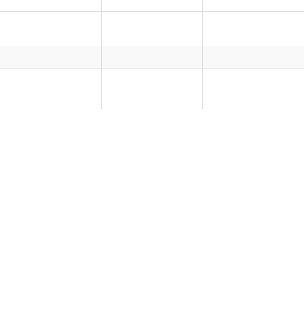
In this runtime, the operators in the execution plan are chained together in a tree, where each non-
leaf operator feeds from one or two child operators. The tree thus comprises nested iterators, and the
records are streamed in a pipelined manner from the top iterator, which pulls from the next iterator
and so on.
Slotted
This is very similar to the interpreted runtime, except that there are additional optimizations regarding
the way in which the records are streamed through the iterators. This results in improvements to both
the performance and memory usage of the query. In effect, this can be thought of as the 'faster
interpreted' runtime.
Compiled
Algorithms are employed to intelligently group the operators in the execution plan in order to
generate new combinations and orders of execution which are optimised for performance and
memory usage. While this should lead to superior performance in most cases (over both the
interpreted and slotted runtimes), it is still under development and does not support all possible
operators or queries (the slotted runtime covers all operators and queries).
Option Description Default?
runtime=interpreted This will force the query planner to use
the interpreted runtime.
This is not used in Enterprise Edition
unless explicitly asked for. It is the only
option for all queries in Community
Edition—it is not necessary to specify
this option in Community Edition.
runtime=slotted This will cause the query planner to
use the slotted runtime.
This is the default option for all
queries which are not supported by
runtime=compiled in Enterprise Edition.
runtime=compiled This will cause the query planner to
use the compiled runtime if it
supports the query. If the compiled
runtime does not support the query,
the planner will fall back to the slotted
runtime.
This is the default option for some
queries in Enterprise Edition.
6.2. Profiling a query
There are two options to choose from when you want to analyze a query by looking at its execution
plan:
EXPLAIN
If you want to see the execution plan but not run the statement, prepend your Cypher statement
with EXPLAIN. The statement will always return an empty result and make no changes to the
database.
PROFILE
If you want to run the statement and see which operators are doing most of the work, use PROFILE.
This will run your statement and keep track of how many rows pass through each operator, and
how much each operator needs to interact with the storage layer to retrieve the necessary data.
Please note that profiling your query uses more resources, so you should not profile unless you are
actively working on a query.
See Execution plans for a detailed explanation of each of the operators contained in an execution
plan.
315

Being explicit about what types and labels you expect relationships and nodes to
have in your query helps Neo4j use the best possible statistical information, which
leads to better execution plans. This means that when you know that a relationship
can only be of a certain type, you should add that to the query. The same goes for
labels, where declaring labels on both the start and end nodes of a relationship
helps Neo4j find the best way to execute the statement.
6.3. Basic query tuning example
We’ll start with a basic example to help you get the hang of profiling queries. The following examples
will use a movies data set.
Let’s start by importing the data:
LOAD CSV WITH HEADERS FROM 'https://neo4j.com/docs/cypher-manual/3.5/csv/query-tuning/movies.csv' AS line
MERGE (m:Movie { title: line.title })
ON CREATE SET m.released = toInteger(line.released), m.tagline = line.tagline
LOAD CSV WITH HEADERS FROM 'https://neo4j.com/docs/cypher-manual/3.5/csv/query-tuning/actors.csv' AS line
MATCH (m:Movie { title: line.title })
MERGE (p:Person { name: line.name })
ON CREATE SET p.born = toInteger(line.born)
MERGE (p)-[:ACTED_IN { roles:split(line.roles, ';')}]->(m)
LOAD CSV WITH HEADERS FROM 'https://neo4j.com/docs/cypher-manual/3.5/csv/query-tuning/directors.csv' AS
line
MATCH (m:Movie { title: line.title })
MERGE (p:Person { name: line.name })
ON CREATE SET p.born = toInteger(line.born)
MERGE (p)-[:DIRECTED]->(m)
Let’s say we want to write a query to find 'Tom Hanks'. The naive way of doing this would be to write
the following:
MATCH (p { name: 'Tom Hanks' })
RETURN p
This query will find the 'Tom Hanks' node but as the number of nodes in the database increase it will
become slower and slower. We can profile the query to find out why that is.
You can learn more about the options for profiling queries in Profiling a query but in this case we’re
going to prefix our query with PROFILE:
PROFILE
MATCH (p { name: 'Tom Hanks' })
RETURN p
316

Compiler CYPHER 3.5
Planner COST
Runtime INTERPRETED
Runtime version 3.5
+-----------------+----------------+------+---------+-----------------+-------------------
+----------------------+-----------+---------------------------+
| Operator | Estimated Rows | Rows | DB Hits | Page Cache Hits | Page Cache Misses | Page Cache Hit
Ratio | Variables | Other |
+-----------------+----------------+------+---------+-----------------+-------------------
+----------------------+-----------+---------------------------+
| +ProduceResults | 16 | 1 | 0 | 0 | 0 |
0.0000 | p | |
| | +----------------+------+---------+-----------------+-------------------
+----------------------+-----------+---------------------------+
| +Filter | 16 | 1 | 163 | 0 | 0 |
0.0000 | p | p.name = $` AUTOSTRING0` |
| | +----------------+------+---------+-----------------+-------------------
+----------------------+-----------+---------------------------+
| +AllNodesScan | 163 | 163 | 164 | 0 | 0 |
0.0000 | p | |
+-----------------+----------------+------+---------+-----------------+-------------------
+----------------------+-----------+---------------------------+
Total database accesses: 327
The first thing to keep in mind when reading execution plans is that you need to read from the bottom
up.
In that vein, starting from the last row, the first thing we notice is that the value in the Rows column
seems high given there is only one node with the name property 'Tom Hanks' in the database. If we
look across to the Operator column we’ll see that AllNodesScan has been used which means that the
query planner scanned through all the nodes in the database.
This seems like an inefficient way of finding 'Tom Hanks' given that we are looking at many nodes that
aren’t even people and therefore aren’t what we’re looking for.
The solution to this problem is that whenever we’re looking for a node we should specify a label to
help the query planner narrow down the search space. For this query we’d need to add a Person label.
MATCH (p:Person { name: 'Tom Hanks' })
RETURN p
This query will be faster than the first one but as the number of people in our database increase we
again notice that the query slows down.
Again we can profile the query to work out why:
PROFILE
MATCH (p:Person { name: 'Tom Hanks' })
RETURN p
317

Compiler CYPHER 3.5
Planner COST
Runtime INTERPRETED
Runtime version 3.5
+------------------+----------------+------+---------+-----------------+-------------------
+----------------------+-----------+---------------------------+
| Operator | Estimated Rows | Rows | DB Hits | Page Cache Hits | Page Cache Misses | Page Cache
Hit Ratio | Variables | Other |
+------------------+----------------+------+---------+-----------------+-------------------
+----------------------+-----------+---------------------------+
| +ProduceResults | 13 | 1 | 0 | 0 | 0 |
0.0000 | p | |
| | +----------------+------+---------+-----------------+-------------------
+----------------------+-----------+---------------------------+
| +Filter | 13 | 1 | 125 | 0 | 0 |
0.0000 | p | p.name = $` AUTOSTRING0` |
| | +----------------+------+---------+-----------------+-------------------
+----------------------+-----------+---------------------------+
| +NodeByLabelScan | 125 | 125 | 126 | 0 | 0 |
0.0000 | p | :Person |
+------------------+----------------+------+---------+-----------------+-------------------
+----------------------+-----------+---------------------------+
Total database accesses: 251
This time the Rows value on the last row has reduced so we’re not scanning some nodes that we were
before which is a good start. The NodeByLabelScan operator indicates that we achieved this by first
doing a linear scan of all the Person nodes in the database.
Once we’ve done that we again scan through all those nodes using the Filter operator, comparing
the name property of each one.
This might be acceptable in some cases but if we’re going to be looking up people by name frequently
then we’ll see better performance if we create an index on the name property for the Person label:
CREATE INDEX ON :Person(name)
Now if we run the query again it will run more quickly:
MATCH (p:Person { name: 'Tom Hanks' })
RETURN p
Let’s profile the query to see why that is:
PROFILE
MATCH (p:Person { name: 'Tom Hanks' })
RETURN p
318

Compiler CYPHER 3.5
Planner COST
Runtime INTERPRETED
Runtime version 3.5
+-----------------+----------------+------+---------+-----------------+-------------------
+----------------------+------------+-----------+---------------+
| Operator | Estimated Rows | Rows | DB Hits | Page Cache Hits | Page Cache Misses | Page Cache Hit
Ratio | Order | Variables | Other |
+-----------------+----------------+------+---------+-----------------+-------------------
+----------------------+------------+-----------+---------------+
| +ProduceResults | 1 | 1 | 0 | 0 | 0 |
0.0000 | p.name ASC | p | |
| | +----------------+------+---------+-----------------+-------------------
+----------------------+------------+-----------+---------------+
| +NodeIndexSeek | 1 | 1 | 2 | 0 | 0 |
0.0000 | p.name ASC | p | :Person(name) |
+-----------------+----------------+------+---------+-----------------+-------------------
+----------------------+------------+-----------+---------------+
Total database accesses: 2
Our execution plan is down to a single row and uses the Node Index Seek operator which does a
schema index seek (see Indexes) to find the appropriate node.
6.4. Index Values and Order
This section describes some more subtle optimizations based on new native index
capabilities
One of the most important and useful ways of optimizing Cypher queries involves creating
appropriate indexes. This is described in more detail in the section on 'Indexes', and demonstrated in
the basic query tuning example. In summary, an index will be based on the combination of a Label
and a property. Any Cypher query that searches for nodes with a specific label and some predicate on
the property (equality, range or existence) will be planned to use the index if the cost planner deems
that to be the most efficient solution.
In order to benefit from some recent enhancements added to Neo4j 3.5, it is useful to understand
when index-backed property lookup and index-backed order by will come into play. In versions of Neo4j
prior to 3.5, the fact that the index contains the property value, and the results are returned in a
specific order, was not used improve the performance of any later part of the query that might
depend on the property value or result order.
Let’s explain how to use these features with a more advanced query tuning example.
6.4.1. Advanced query tuning example
As with the basic query tuning example we’ll use a movies data set to demonstrate how to do some
more advanced query tuning. This time we’ll create the index up-front. If you want to see the effect of
adding an index, refer back to the basic query tuning example. In this example we want to
demonstrate the impact the new native indexes can have on query performance under certain
conditions. In order to benefit from some recent enhancements added to Neo4j 3.5, it is useful to
understand when index-backed property lookup and index-backed order by will come into play.
LOAD CSV WITH HEADERS FROM 'https://neo4j.com/docs/cypher-manual/3.5/csv/query-tuning/movies.csv' AS line
MERGE (m:Movie { title: line.title })
ON CREATE SET m.released = toInteger(line.released), m.tagline = line.tagline
319

LOAD CSV WITH HEADERS FROM 'https://neo4j.com/docs/cypher-manual/3.5/csv/query-tuning/actors.csv' AS line
MATCH (m:Movie { title: line.title })
MERGE (p:Person { name: line.name })
ON CREATE SET p.born = toInteger(line.born)
MERGE (p)-[:ACTED_IN { roles:split(line.roles, ';')}]->(m)
LOAD CSV WITH HEADERS FROM 'https://neo4j.com/docs/cypher-manual/3.5/csv/query-tuning/directors.csv' AS
line
MATCH (m:Movie { title: line.title })
MERGE (p:Person { name: line.name })
ON CREATE SET p.born = toInteger(line.born)
MERGE (p)-[:DIRECTED]->(m)
CREATE INDEX ON :Person(name)
CALL db.awaitIndexes
CALL db.indexes
+---------------------------------------------------------------------------------------------------------
-----------------------------------------------------------------------------+
| description | indexName | tokenNames | properties | state | type
| progress | provider | id | failureMessage |
+---------------------------------------------------------------------------------------------------------
-----------------------------------------------------------------------------+
| "INDEX ON :Person(name)" | "Unnamed index" | ["Person"] | ["name"] | "ONLINE" | "node_label_property"
| 100.0 | {version -> "1.0", key -> "native-btree"} | 1 | "" |
+---------------------------------------------------------------------------------------------------------
-----------------------------------------------------------------------------+
1 row
Index-backed property-lookup
Now that we have a model of movies, actors and directors we can ask a question like 'find persons
with the name Tom that acted in a movie':
MATCH (p:Person)-[:ACTED_IN]->(m:Movie)
WHERE p.name STARTS WITH 'Tom'
RETURN p.name, count(m)
+---------------------------+
| p.name | count(m) |
+---------------------------+
| "Tom Cruise" | 3 |
| "Tom Hanks" | 12 |
| "Tom Skerritt" | 1 |
+---------------------------+
3 rows
We have asked the database to return all the actors with the first name 'Tom'. There are three of them
'Tom Cruise', 'Tom Skerritt' and 'Tom Hanks'. In previous versions of Neo4j, the final clause RETURN p.name
would cause the database to take the node p and look up its properties and return the value of the
property name. In Neo4j 3.5, we can now leverage the fact that indexes store the property values. In
this case, it means that the names can be looked up directly from the index. This allows Cypher to
avoid the second call to the database to find the property, which can save time on very large queries.
If we profile the above query, we see that the NodeIndexScan in the Variables column contains
cached[p.name], which means that p.name is retrieved from the index. We can also see that the
320

Projection has no DB Hits, which means it does not have to access the database again.
PROFILE
MATCH (p:Person)-[:ACTED_IN]->(m:Movie)
WHERE p.name STARTS WITH 'Tom'
RETURN p.name, count(m)
Compiler CYPHER 3.5
Planner COST
Runtime INTERPRETED
Runtime version 3.5
+-----------------------+----------------+------+---------+-----------------+-------------------
+----------------------+------------+----------------------------------
+--------------------------------------------+
| Operator | Estimated Rows | Rows | DB Hits | Page Cache Hits | Page Cache Misses | Page
Cache Hit Ratio | Order | Variables | Other
|
+-----------------------+----------------+------+---------+-----------------+-------------------
+----------------------+------------+----------------------------------
+--------------------------------------------+
| +ProduceResults | 1 | 3 | 0 | 0 | 0 |
0.0000 | p.name ASC | count(m), p.name | |
| | +----------------+------+---------+-----------------+-------------------
+----------------------+------------+----------------------------------
+--------------------------------------------+
| +EagerAggregation | 1 | 3 | 0 | 0 | 0 |
0.0000 | p.name ASC | count(m), p.name | p.name |
| | +----------------+------+---------+-----------------+-------------------
+----------------------+------------+----------------------------------
+--------------------------------------------+
| +Filter | 1 | 16 | 16 | 0 | 0 |
0.0000 | p.name ASC | anon[17], cached[p.name], m, p | m:Movie |
| | +----------------+------+---------+-----------------+-------------------
+----------------------+------------+----------------------------------
+--------------------------------------------+
| +Expand(All) | 1 | 16 | 20 | 0 | 0 |
0.0000 | p.name ASC | anon[17], m -- cached[p.name], p | (p)-[:ACTED_IN]->(m) |
| | +----------------+------+---------+-----------------+-------------------
+----------------------+------------+----------------------------------
+--------------------------------------------+
| +NodeIndexSeekByRange | 1 | 4 | 5 | 0 | 0 |
0.0000 | p.name ASC | cached[p.name], p | :Person(name STARTS WITH $` AUTOSTRING0`) |
+-----------------------+----------------+------+---------+-----------------+-------------------
+----------------------+------------+----------------------------------
+--------------------------------------------+
Total database accesses: 41
If we change the query, such that it can no longer use an index, we will see that there will be no
cached[p.name] in the Variables, and that the Projection now has DB Hits, since it accesses the
database again to retrieve the name.
PROFILE
MATCH (p:Person)-[:ACTED_IN]->(m:Movie)
RETURN p.name, count(m)
321

Compiler CYPHER 3.5
Planner COST
Runtime INTERPRETED
Runtime version 3.5
+-------------------+----------------+------+---------+-----------------+-------------------
+----------------------+------------------+----------------------+
| Operator | Estimated Rows | Rows | DB Hits | Page Cache Hits | Page Cache Misses | Page Cache
Hit Ratio | Variables | Other |
+-------------------+----------------+------+---------+-----------------+-------------------
+----------------------+------------------+----------------------+
| +ProduceResults | 13 | 102 | 0 | 0 | 0 |
0.0000 | count(m), p.name | |
| | +----------------+------+---------+-----------------+-------------------
+----------------------+------------------+----------------------+
| +EagerAggregation | 13 | 102 | 172 | 0 | 0 |
0.0000 | count(m), p.name | p.name |
| | +----------------+------+---------+-----------------+-------------------
+----------------------+------------------+----------------------+
| +Filter | 172 | 172 | 172 | 0 | 0 |
0.0000 | anon[17], m, p | p:Person |
| | +----------------+------+---------+-----------------+-------------------
+----------------------+------------------+----------------------+
| +Expand(All) | 172 | 172 | 210 | 0 | 0 |
0.0000 | anon[17], p -- m | (m)<-[:ACTED_IN]-(p) |
| | +----------------+------+---------+-----------------+-------------------
+----------------------+------------------+----------------------+
| +NodeByLabelScan | 38 | 38 | 39 | 0 | 0 |
0.0000 | m | :Movie |
+-------------------+----------------+------+---------+-----------------+-------------------
+----------------------+------------------+----------------------+
Total database accesses: 593
It is important to note, however, that not all property types are supported, because not all have been
ported to the new native index. In addition some property types, like the spatial type Point, are
indexed in an index that is designed to be approximate and cannot return the values. For non-native
indexes and the spatial type Point, there will still be a second DB access to retrieve those values. In
indexes with mixed values, only those values that cannot be looked up from the index will trigger
another database access action, while the other values will not.
Note also that if you have pre-existing indexes that were build on lucene, upgrading to Neo4j 3.5 is not
sufficient to use the new index. It is necessary to drop and re-create the index in order to port it to the
native index. For information on native index support see the Operations Manual:
•Property types supported by the native index
•Index providers and property types
•Index configuration upgrade considerations
Predicates that can be used to enable this optimization are:
•Existance (WHERE exists(n.name))
•Equality (e.g. WHERE n.name = 'Tom Hanks')
•Range (eg. WHERE n.uid > 1000 AND n.uid < 2000)
•Prefix (eg. WHERE n.name STARTS WITH 'Tom')
•Suffix (eg. WHERE n.name ENDS WITH 'Hanks')
•Substring (eg. WHERE n.name CONTAINS 'a')
322

Index-backed order by
Now consider the following refinement to the query:
MATCH (p:Person)-[:ACTED_IN]->(m:Movie)
WHERE p.name STARTS WITH 'Tom'
RETURN p.name, count(m)
ORDER BY p.name
+---------------------------+
| p.name | count(m) |
+---------------------------+
| "Tom Cruise" | 3 |
| "Tom Hanks" | 12 |
| "Tom Skerritt" | 1 |
+---------------------------+
3 rows
We are asking for the results in ascending alphabetical order. The new native index happens to store
the String properties in ascending alphabetical order, and Cypher knows this. In Neo4j 3.4 and earlier,
Cypher would plan a Sort operation to sort the results, which means building a collection in memory
and running a sort algorithm on it. For large result sets this can be expensive in terms of both
memory and time. In Neo4j 3.5, if you are using the native index, Cypher will recognise that the index
already returns data in the correct order, and skip the Sort operation.
However, indexes storing values of the spatial type Point and non-native indexes cannot be relied on
to return the values in the correct order. This means that for Cypher to enable this optimization, the
query needs a predicate that limits the type of the property to some type that is guaranteed to be in
the right order.
To demonstrate this effect, let’s remove the String prefix predicate so that Cypher no longer knows the
type of the property, and replace it with an existence predicate. Now the database can no longer
guarantee the order. If we profile the query we will see the Sort operation:
PROFILE
MATCH (p:Person)-[:ACTED_IN]->(m:Movie)
USING INDEX p:Person(name)
WHERE exists(p.name)
RETURN p.name, count(m)
ORDER BY p.name
323

Compiler CYPHER 3.5
Planner COST
Runtime INTERPRETED
Runtime version 3.5
+-------------------+----------------+------+---------+-----------------+-------------------
+----------------------+------------+----------------------------------+----------------------+
| Operator | Estimated Rows | Rows | DB Hits | Page Cache Hits | Page Cache Misses | Page Cache
Hit Ratio | Order | Variables | Other |
+-------------------+----------------+------+---------+-----------------+-------------------
+----------------------+------------+----------------------------------+----------------------+
| +ProduceResults | 13 | 102 | 0 | 0 | 0 |
0.0000 | p.name ASC | count(m), p.name | |
| | +----------------+------+---------+-----------------+-------------------
+----------------------+------------+----------------------------------+----------------------+
| +Sort | 13 | 102 | 0 | 0 | 0 |
0.0000 | p.name ASC | count(m), p.name | p.name |
| | +----------------+------+---------+-----------------+-------------------
+----------------------+------------+----------------------------------+----------------------+
| +EagerAggregation | 13 | 102 | 0 | 0 | 0 |
0.0000 | | count(m), p.name | p.name |
| | +----------------+------+---------+-----------------+-------------------
+----------------------+------------+----------------------------------+----------------------+
| +Filter | 172 | 172 | 172 | 0 | 0 |
0.0000 | | anon[17], cached[p.name], m, p | m:Movie |
| | +----------------+------+---------+-----------------+-------------------
+----------------------+------------+----------------------------------+----------------------+
| +Expand(All) | 172 | 172 | 297 | 0 | 0 |
0.0000 | | anon[17], m -- cached[p.name], p | (p)-[:ACTED_IN]->(m) |
| | +----------------+------+---------+-----------------+-------------------
+----------------------+------------+----------------------------------+----------------------+
| +NodeIndexScan | 125 | 125 | 127 | 0 | 0 |
0.0000 | | cached[p.name], p | :Person(name) |
+-------------------+----------------+------+---------+-----------------+-------------------
+----------------------+------------+----------------------------------+----------------------+
Total database accesses: 596
We can also see a new column in the profile, that was added in Neo4j 3.5: Order. This column
describes the order of rows after each operator. We see that the order is undefined until the Sort
operator. Now if we add back the predicate that gives us the property type information, we will see
the Sort operation is no longer there:
PROFILE
MATCH (p:Person)-[:ACTED_IN]->(m:Movie)
WHERE p.name STARTS WITH 'Tom'
RETURN p.name, count(m)
ORDER BY p.name
324

Compiler CYPHER 3.5
Planner COST
Runtime INTERPRETED
Runtime version 3.5
+-----------------------+----------------+------+---------+-----------------+-------------------
+----------------------+------------+----------------------------------
+--------------------------------------------+
| Operator | Estimated Rows | Rows | DB Hits | Page Cache Hits | Page Cache Misses | Page
Cache Hit Ratio | Order | Variables | Other
|
+-----------------------+----------------+------+---------+-----------------+-------------------
+----------------------+------------+----------------------------------
+--------------------------------------------+
| +ProduceResults | 1 | 3 | 0 | 0 | 0 |
0.0000 | p.name ASC | count(m), p.name | |
| | +----------------+------+---------+-----------------+-------------------
+----------------------+------------+----------------------------------
+--------------------------------------------+
| +EagerAggregation | 1 | 3 | 0 | 0 | 0 |
0.0000 | p.name ASC | count(m), p.name | p.name |
| | +----------------+------+---------+-----------------+-------------------
+----------------------+------------+----------------------------------
+--------------------------------------------+
| +Filter | 1 | 16 | 16 | 0 | 0 |
0.0000 | p.name ASC | anon[17], cached[p.name], m, p | m:Movie |
| | +----------------+------+---------+-----------------+-------------------
+----------------------+------------+----------------------------------
+--------------------------------------------+
| +Expand(All) | 1 | 16 | 20 | 0 | 0 |
0.0000 | p.name ASC | anon[17], m -- cached[p.name], p | (p)-[:ACTED_IN]->(m) |
| | +----------------+------+---------+-----------------+-------------------
+----------------------+------------+----------------------------------
+--------------------------------------------+
| +NodeIndexSeekByRange | 1 | 4 | 5 | 0 | 0 |
0.0000 | p.name ASC | cached[p.name], p | :Person(name STARTS WITH $` AUTOSTRING0`) |
+-----------------------+----------------+------+---------+-----------------+-------------------
+----------------------+------------+----------------------------------
+--------------------------------------------+
Total database accesses: 41
We also see that the Order column contains p.name ASC from the index seek operation, meaning that
the rows are ordered by p.name in ascending order.
Index-backed order by can just as well be used for queries that expect their results is descending
order, but with slightly lower performance.
Restrictions
The optimization can only work on new native indexes and only if we query for a specific type in order
to rule out the spatial type Point. Predicates that can be used to enable this optimization are:
•Equality (e.g. WHERE n.name = 'Tom Hanks')
•Range (eg. WHERE n.uid > 1000 AND n.uid < 2000)
•Prefix (eg. WHERE n.name STARTS WITH 'Tom')
•Suffix (eg. WHERE n.name ENDS WITH 'Hanks')
•Substring (eg. WHERE n.name CONTAINS 'a')
Predicates that will not work:
•Existence (eg. WHERE exists(n.email)) because no property type information is given
325
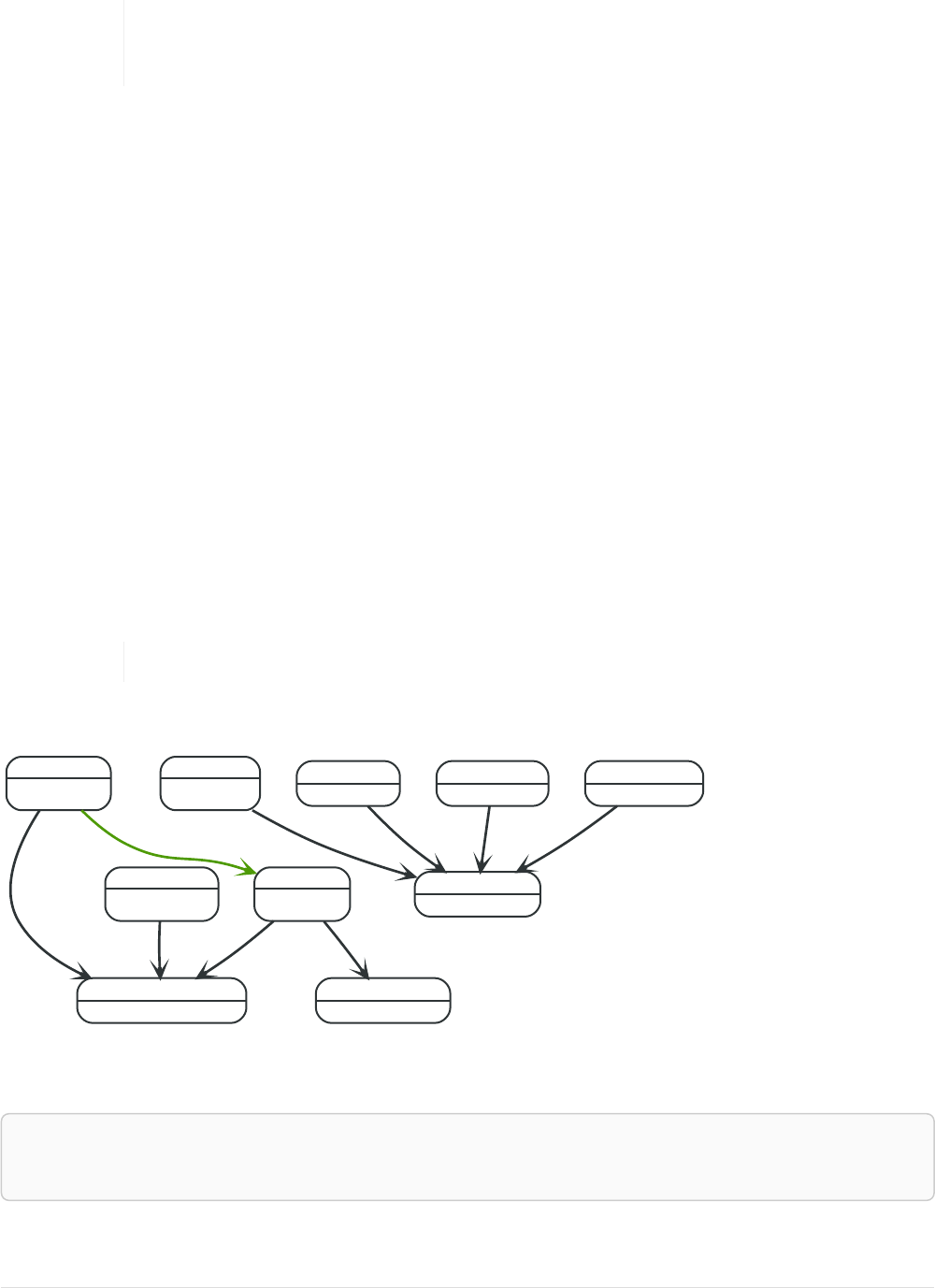
6.5. Planner hints and the USING keyword
A planner hint is used to influence the decisions of the planner when building an execution
plan for a query. Planner hints are specified in a query with the USING keyword.
Forcing planner behavior is an advanced feature, and should be used with caution
by experienced developers and/or database administrators only, as it may cause
queries to perform poorly.
•Introduction
•Index hints
•Scan hints
•Join hints
•PERIODIC COMMIT query hint
6.5.1. Introduction
When executing a query, Neo4j needs to decide where in the query graph to start matching. This is
done by looking at the MATCH clause and the WHERE conditions and using that information to find useful
indexes, or other starting points.
However, the selected index might not always be the best choice. Sometimes multiple indexes are
possible candidates, and the query planner picks the suboptimal one from a performance point of
view. Moreover, in some circumstances (albeit rarely) it is better not to use an index at all.
Neo4j can be forced to use a specific starting point through the USING keyword. This is called giving a
planner hint. There are four types of planner hints: index hints, scan hints, join hints, and the PERIODIC
COMMIT query hint.
You cannot use planner hints if your query has a START clause.
The following graph is used for the examples below:
Scientist
name = 'Liskov'
born = 1939
Science
name = 'Computer Science'
RESEARCHED
Scientist
name = 'Wing'
born = 1956
KNOWS
RESEARCHED
Science
name = 'Engineering'
RESEARCHED
Scientist
name = 'Conway'
born = 1938
RESEARCHED
Science
name = 'Chemistry'
Scientist
name = 'Curie'
born = 1867
RESEARCHED
Scientist
name = 'Arden'
RESEARCHED
Scientist
name = 'Franklin'
RESEARCHED
Scientist
name = 'Harrison'
RESEARCHED
Figure 28. Graph
Query
MATCH (liskov:Scientist { name:'Liskov' })-[:KNOWS]->(wing:Scientist)-[:RESEARCHED]->(cs:Science {
name:'Computer Science' })<-[:RESEARCHED]-(conway:Scientist { name: 'Conway' })
RETURN 1 AS column
The following query will be used in some of the examples on this page. It has intentionally been
326

constructed in such a way that the statistical information will be inaccurate for the particular subgraph
that this query matches. For this reason, it can be improved by supplying planner hints.
Query plan
Compiler CYPHER 3.5
Planner COST
Runtime COMPILED
Runtime version 3.5
+-----------------+----------------+------+---------+-----------------+-------------------
+----------------------+-----------+-----------------
+-------------------------------------------------------------------
+--------------------------------------------------------------------------------+
| Operator | Estimated Rows | Rows | DB Hits | Page Cache Hits | Page Cache Misses | Page Cache Hit
Ratio | Time (ms) | Order | Variables |
Other |
+-----------------+----------------+------+---------+-----------------+-------------------
+----------------------+-----------+-----------------
+-------------------------------------------------------------------
+--------------------------------------------------------------------------------+
| +ProduceResults | 0 | 1 | 0 | 5 | 1 |
0.8333 | 0.117 | liskov.name ASC | anon[126], anon[43], anon[70], column, conway, cs, liskov, wing |
|
| | +----------------+------+---------+-----------------+-------------------
+----------------------+-----------+-----------------
+-------------------------------------------------------------------
+--------------------------------------------------------------------------------+
| +Projection | 0 | 1 | 0 | 5 | 1 |
0.8333 | 0.121 | liskov.name ASC | column -- anon[126], anon[43], anon[70], conway, cs, liskov, wing |
{column : $` AUTOINT3`} |
| | +----------------+------+---------+-----------------+-------------------
+----------------------+-----------+-----------------
+-------------------------------------------------------------------
+--------------------------------------------------------------------------------+
| +Filter | 0 | 6 | 5 | 15 | 3 |
0.8333 | 0.141 | liskov.name ASC | anon[126], anon[43], anon[70], conway, cs, liskov, wing |
conway:Scientist; not `anon[126]` = `anon[70]`; conway.name = $` AUTOSTRING2` |
| | +----------------+------+---------+-----------------+-------------------
+----------------------+-----------+-----------------
+-------------------------------------------------------------------
+--------------------------------------------------------------------------------+
| +Expand(All) | 0 | 3 | 4 | 5 | 1 |
0.8333 | 0.173 | liskov.name ASC | anon[126], conway -- anon[43], anon[70], cs, liskov, wing |
(cs)<-[:RESEARCHED]-(conway) |
| | +----------------+------+---------+-----------------+-------------------
+----------------------+-----------+-----------------
+-------------------------------------------------------------------
+--------------------------------------------------------------------------------+
| +Filter | 0 | 3 | 4 | 9 | 2 |
0.8182 | 0.319 | liskov.name ASC | anon[43], anon[70], cs, liskov, wing |
cs:Science; cs.name = $` AUTOSTRING1` |
| | +----------------+------+---------+-----------------+-------------------
+----------------------+-----------+-----------------
+-------------------------------------------------------------------
+--------------------------------------------------------------------------------+
| +Expand(All) | 0 | 2 | 3 | 5 | 1 |
0.8333 | 0.386 | liskov.name ASC | anon[70], cs -- anon[43], liskov, wing |
(wing)-[:RESEARCHED]->(cs) |
| | +----------------+------+---------+-----------------+-------------------
+----------------------+-----------+-----------------
+-------------------------------------------------------------------
+--------------------------------------------------------------------------------+
| +Filter | 0 | 1 | 1 | 5 | 1 |
0.8333 | 0.410 | liskov.name ASC | anon[43], liskov, wing |
wing:Scientist |
| | +----------------+------+---------+-----------------+-------------------
+----------------------+-----------+-----------------
+-------------------------------------------------------------------
+--------------------------------------------------------------------------------+
| +Expand(All) | 0 | 1 | 2 | 5 | 1 |
0.8333 | 1.023 | liskov.name ASC | anon[43], wing -- liskov |
(liskov)-[:KNOWS]->(wing) |
| | +----------------+------+---------+-----------------+-------------------
+----------------------+-----------+-----------------
327

+-------------------------------------------------------------------
+--------------------------------------------------------------------------------+
| +NodeIndexSeek | 1 | 1 | 2 | 5 | 1 |
0.8333 | 2.573 | liskov.name ASC | liskov |
:Scientist(name) |
+-----------------+----------------+------+---------+-----------------+-------------------
+----------------------+-----------+-----------------
+-------------------------------------------------------------------
+--------------------------------------------------------------------------------+
Total database accesses: 21
6.5.2. Index hints
Index hints are used to specify which index, if any, the planner should use as a starting point. This can
be beneficial in cases where the index statistics are not accurate for the specific values that the query
at hand is known to use, which would result in the planner picking a non-optimal index. To supply an
index hint, use USING INDEX variable:Label(property) or USING INDEX SEEK variable:Label(property)
after the applicable MATCH clause.
It is possible to supply several index hints, but keep in mind that several starting points will require the
use of a potentially expensive join later in the query plan.
Query using an index hint
The query above will not naturally pick an index to solve the plan. This is because the graph is very
small, and label scans are faster for small databases. In general, however, query performance is
ranked by the dbhit metric, and we see that using an index is slightly better for this query.
Query
MATCH (liskov:Scientist { name:'Liskov' })-[:KNOWS]->(wing:Scientist)-[:RESEARCHED]->(cs:Science {
name:'Computer Science' })<-[:RESEARCHED]-(conway:Scientist { name: 'Conway' })
USING INDEX liskov:Scientist(name)
RETURN liskov.born AS column
Returns the year 'Barbara Liskov' was born.
Query plan
Compiler CYPHER 3.5
Planner COST
Runtime COMPILED
Runtime version 3.5
+-----------------+----------------+------+---------+-----------------+-------------------
+----------------------+-----------+-----------------
+-------------------------------------------------------------------
+--------------------------------------------------------------------------------+
| Operator | Estimated Rows | Rows | DB Hits | Page Cache Hits | Page Cache Misses | Page Cache Hit
Ratio | Time (ms) | Order | Variables |
Other |
+-----------------+----------------+------+---------+-----------------+-------------------
+----------------------+-----------+-----------------
+-------------------------------------------------------------------
+--------------------------------------------------------------------------------+
| +ProduceResults | 0 | 1 | 0 | 6 | 0 |
1.0000 | 0.081 | liskov.name ASC | anon[126], anon[43], anon[70], column, conway, cs, liskov, wing |
|
| | +----------------+------+---------+-----------------+-------------------
+----------------------+-----------+-----------------
+-------------------------------------------------------------------
+--------------------------------------------------------------------------------+
| +Projection | 0 | 1 | 1 | 6 | 0 |
1.0000 | 0.089 | liskov.name ASC | column -- anon[126], anon[43], anon[70], conway, cs, liskov, wing |
328

{column : liskov.born} |
| | +----------------+------+---------+-----------------+-------------------
+----------------------+-----------+-----------------
+-------------------------------------------------------------------
+--------------------------------------------------------------------------------+
| +Filter | 0 | 6 | 5 | 18 | 0 |
1.0000 | 0.106 | liskov.name ASC | anon[126], anon[43], anon[70], conway, cs, liskov, wing |
conway:Scientist; not `anon[126]` = `anon[70]`; conway.name = $` AUTOSTRING2` |
| | +----------------+------+---------+-----------------+-------------------
+----------------------+-----------+-----------------
+-------------------------------------------------------------------
+--------------------------------------------------------------------------------+
| +Expand(All) | 0 | 3 | 4 | 6 | 0 |
1.0000 | 0.129 | liskov.name ASC | anon[126], conway -- anon[43], anon[70], cs, liskov, wing |
(cs)<-[:RESEARCHED]-(conway) |
| | +----------------+------+---------+-----------------+-------------------
+----------------------+-----------+-----------------
+-------------------------------------------------------------------
+--------------------------------------------------------------------------------+
| +Filter | 0 | 3 | 4 | 11 | 0 |
1.0000 | 0.218 | liskov.name ASC | anon[43], anon[70], cs, liskov, wing |
cs:Science; cs.name = $` AUTOSTRING1` |
| | +----------------+------+---------+-----------------+-------------------
+----------------------+-----------+-----------------
+-------------------------------------------------------------------
+--------------------------------------------------------------------------------+
| +Expand(All) | 0 | 2 | 3 | 6 | 0 |
1.0000 | 0.235 | liskov.name ASC | anon[70], cs -- anon[43], liskov, wing |
(wing)-[:RESEARCHED]->(cs) |
| | +----------------+------+---------+-----------------+-------------------
+----------------------+-----------+-----------------
+-------------------------------------------------------------------
+--------------------------------------------------------------------------------+
| +Filter | 0 | 1 | 1 | 6 | 0 |
1.0000 | 0.248 | liskov.name ASC | anon[43], liskov, wing |
wing:Scientist |
| | +----------------+------+---------+-----------------+-------------------
+----------------------+-----------+-----------------
+-------------------------------------------------------------------
+--------------------------------------------------------------------------------+
| +Expand(All) | 0 | 1 | 2 | 6 | 0 |
1.0000 | 0.347 | liskov.name ASC | anon[43], wing -- liskov |
(liskov)-[:KNOWS]->(wing) |
| | +----------------+------+---------+-----------------+-------------------
+----------------------+-----------+-----------------
+-------------------------------------------------------------------
+--------------------------------------------------------------------------------+
| +NodeIndexSeek | 1 | 1 | 2 | 6 | 0 |
1.0000 | 0.528 | liskov.name ASC | liskov |
:Scientist(name) |
+-----------------+----------------+------+---------+-----------------+-------------------
+----------------------+-----------+-----------------
+-------------------------------------------------------------------
+--------------------------------------------------------------------------------+
Total database accesses: 22
Query using an index seek hint
Similar to the index (scan) hint, but an index seek will be used rather than an index scan. Index seeks
require no post filtering, they are most efficient when a relatively small number of nodes have the
specified value on the queried property.
Query
MATCH (liskov:Scientist { name:'Liskov' })-[:KNOWS]->(wing:Scientist)-[:RESEARCHED]->(cs:Science {
name:'Computer Science' })<-[:RESEARCHED]-(conway:Scientist { name: 'Conway' })
USING INDEX SEEK liskov:Scientist(name)
RETURN liskov.born AS column
Returns the year 'Barbara Liskov' was born.
Query plan
329

Compiler CYPHER 3.5
Planner COST
Runtime COMPILED
Runtime version 3.5
+-----------------+----------------+------+---------+-----------------+-------------------
+----------------------+-----------+-----------------
+-------------------------------------------------------------------
+--------------------------------------------------------------------------------+
| Operator | Estimated Rows | Rows | DB Hits | Page Cache Hits | Page Cache Misses | Page Cache Hit
Ratio | Time (ms) | Order | Variables |
Other |
+-----------------+----------------+------+---------+-----------------+-------------------
+----------------------+-----------+-----------------
+-------------------------------------------------------------------
+--------------------------------------------------------------------------------+
| +ProduceResults | 0 | 1 | 0 | 6 | 0 |
1.0000 | 0.076 | liskov.name ASC | anon[126], anon[43], anon[70], column, conway, cs, liskov, wing |
|
| | +----------------+------+---------+-----------------+-------------------
+----------------------+-----------+-----------------
+-------------------------------------------------------------------
+--------------------------------------------------------------------------------+
| +Projection | 0 | 1 | 1 | 6 | 0 |
1.0000 | 0.085 | liskov.name ASC | column -- anon[126], anon[43], anon[70], conway, cs, liskov, wing |
{column : liskov.born} |
| | +----------------+------+---------+-----------------+-------------------
+----------------------+-----------+-----------------
+-------------------------------------------------------------------
+--------------------------------------------------------------------------------+
| +Filter | 0 | 6 | 5 | 18 | 0 |
1.0000 | 0.102 | liskov.name ASC | anon[126], anon[43], anon[70], conway, cs, liskov, wing |
conway:Scientist; not `anon[126]` = `anon[70]`; conway.name = $` AUTOSTRING2` |
| | +----------------+------+---------+-----------------+-------------------
+----------------------+-----------+-----------------
+-------------------------------------------------------------------
+--------------------------------------------------------------------------------+
| +Expand(All) | 0 | 3 | 4 | 6 | 0 |
1.0000 | 0.128 | liskov.name ASC | anon[126], conway -- anon[43], anon[70], cs, liskov, wing |
(cs)<-[:RESEARCHED]-(conway) |
| | +----------------+------+---------+-----------------+-------------------
+----------------------+-----------+-----------------
+-------------------------------------------------------------------
+--------------------------------------------------------------------------------+
| +Filter | 0 | 3 | 4 | 11 | 0 |
1.0000 | 0.221 | liskov.name ASC | anon[43], anon[70], cs, liskov, wing |
cs:Science; cs.name = $` AUTOSTRING1` |
| | +----------------+------+---------+-----------------+-------------------
+----------------------+-----------+-----------------
+-------------------------------------------------------------------
+--------------------------------------------------------------------------------+
| +Expand(All) | 0 | 2 | 3 | 6 | 0 |
1.0000 | 0.245 | liskov.name ASC | anon[70], cs -- anon[43], liskov, wing |
(wing)-[:RESEARCHED]->(cs) |
| | +----------------+------+---------+-----------------+-------------------
+----------------------+-----------+-----------------
+-------------------------------------------------------------------
+--------------------------------------------------------------------------------+
| +Filter | 0 | 1 | 1 | 6 | 0 |
1.0000 | 0.258 | liskov.name ASC | anon[43], liskov, wing |
wing:Scientist |
| | +----------------+------+---------+-----------------+-------------------
+----------------------+-----------+-----------------
+-------------------------------------------------------------------
+--------------------------------------------------------------------------------+
| +Expand(All) | 0 | 1 | 2 | 6 | 0 |
1.0000 | 0.355 | liskov.name ASC | anon[43], wing -- liskov |
(liskov)-[:KNOWS]->(wing) |
| | +----------------+------+---------+-----------------+-------------------
+----------------------+-----------+-----------------
+-------------------------------------------------------------------
+--------------------------------------------------------------------------------+
| +NodeIndexSeek | 1 | 1 | 2 | 6 | 0 |
1.0000 | 0.544 | liskov.name ASC | liskov |
:Scientist(name) |
+-----------------+----------------+------+---------+-----------------+-------------------
+----------------------+-----------+-----------------
330

+-------------------------------------------------------------------
+--------------------------------------------------------------------------------+
Total database accesses: 22
Query using multiple index hints
Supplying one index hint changed the starting point of the query, but the plan is still linear, meaning it
only has one starting point. If we give the planner yet another index hint, we force it to use two
starting points, one at each end of the match. It will then join these two branches using a join
operator.
Query
MATCH (liskov:Scientist { name:'Liskov' })-[:KNOWS]->(wing:Scientist)-[:RESEARCHED]->(cs:Science {
name:'Computer Science' })<-[:RESEARCHED]-(conway:Scientist { name: 'Conway' })
USING INDEX liskov:Scientist(name)
USING INDEX conway:Scientist(name)
RETURN liskov.born AS column
Returns the year 'Barbara Liskov' was born, using a slightly better plan.
Query plan
Compiler CYPHER 3.5
Planner COST
Runtime COMPILED
Runtime version 3.5
+---------------------+----------------+------+---------+-----------------+-------------------
+----------------------+-----------+-----------------
+-------------------------------------------------------------------
+----------------------------------------+
| Operator | Estimated Rows | Rows | DB Hits | Page Cache Hits | Page Cache Misses | Page Cache
Hit Ratio | Time (ms) | Order | Variables
| Other |
+---------------------+----------------+------+---------+-----------------+-------------------
+----------------------+-----------+-----------------
+-------------------------------------------------------------------
+----------------------------------------+
| +ProduceResults | 0 | 1 | 0 | 6 | 1 |
0.8571 | 0.086 | cs.name ASC | anon[126], anon[43], anon[70], column, conway, cs, liskov, wing |
|
| | +----------------+------+---------+-----------------+-------------------
+----------------------+-----------+-----------------
+-------------------------------------------------------------------
+----------------------------------------+
| +Projection | 0 | 1 | 1 | 6 | 1 |
0.8571 | 0.107 | cs.name ASC | column -- anon[126], anon[43], anon[70], conway, cs, liskov, wing |
{column : liskov.born} |
| | +----------------+------+---------+-----------------+-------------------
+----------------------+-----------+-----------------
+-------------------------------------------------------------------
+----------------------------------------+
| +Filter | 0 | 1 | 0 | 6 | 1 |
0.8571 | 0.111 | cs.name ASC | anon[126], anon[43], anon[70], conway, cs, liskov, wing |
not `anon[126]` = `anon[70]` |
| | +----------------+------+---------+-----------------+-------------------
+----------------------+-----------+-----------------
+-------------------------------------------------------------------
+----------------------------------------+
| +NodeHashJoin | 0 | 1 | 0 | 11 | 1 |
0.9167 | 0.585 | cs.name ASC | anon[43], anon[70], liskov, wing -- anon[126], conway, cs |
cs |
| |\ +----------------+------+---------+-----------------+-------------------
+----------------------+-----------+-----------------
+-------------------------------------------------------------------
+----------------------------------------+
| | +Expand(Into) | 0 | 1 | 2 | 6 | 1 |
331

0.8571 | 0.954 | cs.name ASC | anon[126] -- conway, cs |
(cs)<-[:RESEARCHED]-(conway) |
| | | +----------------+------+---------+-----------------+-------------------
+----------------------+-----------+-----------------
+-------------------------------------------------------------------
+----------------------------------------+
| | +CartesianProduct | 1 | 1 | 0 | 6 | 1 |
0.8571 | 0.958 | cs.name ASC | cs -- conway |
|
| | |\ +----------------+------+---------+-----------------+-------------------
+----------------------+-----------+-----------------
+-------------------------------------------------------------------
+----------------------------------------+
| | | +NodeIndexSeek | 1 | 1 | 2 | 6 | 1 |
0.8571 | 0.995 | conway.name ASC | conway |
:Scientist(name) |
| | | +----------------+------+---------+-----------------+-------------------
+----------------------+-----------+-----------------
+-------------------------------------------------------------------
+----------------------------------------+
| | +NodeIndexSeek | 1 | 1 | 2 | 6 | 1 |
0.8571 | 1.065 | cs.name ASC | cs |
:Science(name) |
| | +----------------+------+---------+-----------------+-------------------
+----------------------+-----------+-----------------
+-------------------------------------------------------------------
+----------------------------------------+
| +Filter | 0 | 3 | 4 | 10 | 0 |
1.0000 | 0.671 | liskov.name ASC | anon[43], anon[70], cs, liskov, wing |
cs:Science; cs.name = $` AUTOSTRING1` |
| | +----------------+------+---------+-----------------+-------------------
+----------------------+-----------+-----------------
+-------------------------------------------------------------------
+----------------------------------------+
| +Expand(All) | 0 | 2 | 3 | 5 | 0 |
1.0000 | 0.701 | liskov.name ASC | anon[70], cs -- anon[43], liskov, wing |
(wing)-[:RESEARCHED]->(cs) |
| | +----------------+------+---------+-----------------+-------------------
+----------------------+-----------+-----------------
+-------------------------------------------------------------------
+----------------------------------------+
| +Filter | 0 | 1 | 1 | 5 | 0 |
1.0000 | 0.714 | liskov.name ASC | anon[43], liskov, wing |
wing:Scientist |
| | +----------------+------+---------+-----------------+-------------------
+----------------------+-----------+-----------------
+-------------------------------------------------------------------
+----------------------------------------+
| +Expand(All) | 0 | 1 | 2 | 5 | 0 |
1.0000 | 0.824 | liskov.name ASC | anon[43], wing -- liskov |
(liskov)-[:KNOWS]->(wing) |
| | +----------------+------+---------+-----------------+-------------------
+----------------------+-----------+-----------------
+-------------------------------------------------------------------
+----------------------------------------+
| +NodeIndexSeek | 1 | 1 | 2 | 5 | 0 |
1.0000 | 1.022 | liskov.name ASC | liskov |
:Scientist(name) |
+---------------------+----------------+------+---------+-----------------+-------------------
+----------------------+-----------+-----------------
+-------------------------------------------------------------------
+----------------------------------------+
Total database accesses: 19
6.5.3. Scan hints
If your query matches large parts of an index, it might be faster to scan the label and filter out nodes
that do not match. To do this, you can use USING SCAN variable:Label after the applicable MATCH
clause. This will force Cypher to not use an index that could have been used, and instead do a label
scan.
332

Hinting a label scan
If the best performance is to be had by scanning all nodes in a label and then filtering on that set, use
USING SCAN.
Query
MATCH (s:Scientist)
USING SCAN s:Scientist
WHERE s.born < 1939
RETURN s.born AS column
Returns all scientists born before '1939'.
Query plan
Compiler CYPHER 3.5
Planner COST
Runtime SLOTTED
Runtime version 3.5
+------------------+----------------+------+---------+-----------------+-------------------
+----------------------+-------------+------------------------+
| Operator | Estimated Rows | Rows | DB Hits | Page Cache Hits | Page Cache Misses | Page Cache
Hit Ratio | Variables | Other |
+------------------+----------------+------+---------+-----------------+-------------------
+----------------------+-------------+------------------------+
| +ProduceResults | 2 | 2 | 0 | 2 | 0 |
1.0000 | column, s | |
| | +----------------+------+---------+-----------------+-------------------
+----------------------+-------------+------------------------+
| +Projection | 2 | 2 | 2 | 2 | 0 |
1.0000 | column -- s | {column : s.born} |
| | +----------------+------+---------+-----------------+-------------------
+----------------------+-------------+------------------------+
| +Filter | 2 | 2 | 7 | 2 | 0 |
1.0000 | s | s.born < $` AUTOINT0` |
| | +----------------+------+---------+-----------------+-------------------
+----------------------+-------------+------------------------+
| +NodeByLabelScan | 7 | 7 | 8 | 3 | 0 |
1.0000 | s | :Scientist |
+------------------+----------------+------+---------+-----------------+-------------------
+----------------------+-------------+------------------------+
Total database accesses: 17
6.5.4. Join hints
Join hints are the most advanced type of hints, and are not used to find starting points for the query
execution plan, but to enforce that joins are made at specified points. This implies that there has to be
more than one starting point (leaf) in the plan, in order for the query to be able to join the two
branches ascending from these leaves. Due to this nature, joins, and subsequently join hints, will force
the planner to look for additional starting points, and in the case where there are no more good ones,
potentially pick a very bad starting point. This will negatively affect query performance. In other cases,
the hint might force the planner to pick a seemingly bad starting point, which in reality proves to be a
very good one.
Hinting a join on a single node
In the example above using multiple index hints, we saw that the planner chose to do a join on the cs
node. This means that the relationship between wing and cs was traversed in the outgoing direction,
which is better statistically because the pattern ()-[:RESEARCHED]→(:Science) is more common than
the pattern (:Scientist)-[:RESEARCHED]→(). However, in the actual graph, the cs node only has two
333

such relationships, so expanding from it will be beneficial to expanding from the wing node. We can
force the join to happen on wing instead with a join hint.
Query
MATCH (liskov:Scientist { name:'Liskov' })-[:KNOWS]->(wing:Scientist)-[:RESEARCHED]->(cs:Science {
name:'Computer Science' })<-[:RESEARCHED]-(conway:Scientist { name: 'Conway' })
USING INDEX liskov:Scientist(name)
USING INDEX conway:Scientist(name)
USING JOIN ON wing
RETURN wing.born AS column
Returns the birth date of 'Jeanette Wing', using a slightly better plan.
Query plan
Compiler CYPHER 3.5
Planner COST
Runtime COMPILED
Runtime version 3.5
+---------------------+----------------+------+---------+-----------------+-------------------
+----------------------+-----------+-----------------
+-------------------------------------------------------------------+------------------------------+
| Operator | Estimated Rows | Rows | DB Hits | Page Cache Hits | Page Cache Misses | Page Cache
Hit Ratio | Time (ms) | Order | Variables
| Other |
+---------------------+----------------+------+---------+-----------------+-------------------
+----------------------+-----------+-----------------
+-------------------------------------------------------------------+------------------------------+
| +ProduceResults | 0 | 1 | 0 | 7 | 0 |
1.0000 | 0.147 | cs.name ASC | anon[126], anon[43], anon[70], column, conway, cs, liskov, wing |
|
| | +----------------+------+---------+-----------------+-------------------
+----------------------+-----------+-----------------
+-------------------------------------------------------------------+------------------------------+
| +Projection | 0 | 1 | 1 | 7 | 0 |
1.0000 | 0.212 | cs.name ASC | column -- anon[126], anon[43], anon[70], conway, cs, liskov, wing |
{column : wing.born} |
| | +----------------+------+---------+-----------------+-------------------
+----------------------+-----------+-----------------
+-------------------------------------------------------------------+------------------------------+
| +NodeHashJoin | 0 | 1 | 0 | 16 | 0 |
1.0000 | 0.726 | cs.name ASC | anon[43], liskov -- anon[126], anon[70], conway, cs, wing |
wing |
| |\ +----------------+------+---------+-----------------+-------------------
+----------------------+-----------+-----------------
+-------------------------------------------------------------------+------------------------------+
| | +Filter | 1 | 2 | 0 | 19 | 0 |
1.0000 | 0.259 | | anon[126], anon[70], conway, cs, wing |
not `anon[126]` = `anon[70]` |
| | | +----------------+------+---------+-----------------+-------------------
+----------------------+-----------+-----------------
+-------------------------------------------------------------------+------------------------------+
| | +Expand(All) | 1 | 3 | 4 | 7 | 0 |
1.0000 | 0.277 | cs.name ASC | anon[70], wing -- anon[126], conway, cs |
(cs)<-[:RESEARCHED]-(wing) |
| | | +----------------+------+---------+-----------------+-------------------
+----------------------+-----------+-----------------
+-------------------------------------------------------------------+------------------------------+
| | +Expand(Into) | 0 | 1 | 2 | 7 | 0 |
1.0000 | 0.347 | cs.name ASC | anon[126] -- conway, cs |
(cs)<-[:RESEARCHED]-(conway) |
| | | +----------------+------+---------+-----------------+-------------------
+----------------------+-----------+-----------------
+-------------------------------------------------------------------+------------------------------+
| | +CartesianProduct | 1 | 1 | 0 | 7 | 0 |
1.0000 | 0.350 | cs.name ASC | cs -- conway |
|
| | |\ +----------------+------+---------+-----------------+-------------------
+----------------------+-----------+-----------------
+-------------------------------------------------------------------+------------------------------+
| | | +NodeIndexSeek | 1 | 1 | 2 | 7 | 0 |
334

1.0000 | 0.386 | conway.name ASC | conway |
:Scientist(name) |
| | | +----------------+------+---------+-----------------+-------------------
+----------------------+-----------+-----------------
+-------------------------------------------------------------------+------------------------------+
| | +NodeIndexSeek | 1 | 1 | 2 | 7 | 0 |
1.0000 | 0.446 | cs.name ASC | cs |
:Science(name) |
| | +----------------+------+---------+-----------------+-------------------
+----------------------+-----------+-----------------
+-------------------------------------------------------------------+------------------------------+
| +Filter | 0 | 1 | 1 | 3 | 0 |
1.0000 | 0.493 | liskov.name ASC | anon[43], liskov, wing |
wing:Scientist |
| | +----------------+------+---------+-----------------+-------------------
+----------------------+-----------+-----------------
+-------------------------------------------------------------------+------------------------------+
| +Expand(All) | 0 | 1 | 2 | 3 | 0 |
1.0000 | 0.612 | liskov.name ASC | anon[43], wing -- liskov |
(liskov)-[:KNOWS]->(wing) |
| | +----------------+------+---------+-----------------+-------------------
+----------------------+-----------+-----------------
+-------------------------------------------------------------------+------------------------------+
| +NodeIndexSeek | 1 | 1 | 2 | 3 | 0 |
1.0000 | 0.877 | liskov.name ASC | liskov |
:Scientist(name) |
+---------------------+----------------+------+---------+-----------------+-------------------
+----------------------+-----------+-----------------
+-------------------------------------------------------------------+------------------------------+
Total database accesses: 16
Hinting a join on multiple nodes
The query planner can be made to produce a join between several specific points. This requires the
query to expand from the same node from several directions.
Query
MATCH (liskov:Scientist { name:'Liskov' })-[:KNOWS]->(wing:Scientist { name:'Wing' })-[:RESEARCHED]-
>(cs:Science { name:'Computer Science' })<-[:RESEARCHED]-(liskov)
USING INDEX liskov:Scientist(name)
USING JOIN ON liskov, cs
RETURN wing.born AS column
Returns the birth date of 'Jeanette Wing'.
Query plan
Compiler CYPHER 3.5
Planner COST
Runtime COMPILED
Runtime version 3.5
+---------------------+----------------+------+---------+-----------------+-------------------
+----------------------+-----------+-----------------
+-----------------------------------------------------------
+----------------------------------------------+
| Operator | Estimated Rows | Rows | DB Hits | Page Cache Hits | Page Cache Misses | Page Cache
Hit Ratio | Time (ms) | Order | Variables |
Other |
+---------------------+----------------+------+---------+-----------------+-------------------
+----------------------+-----------+-----------------
+-----------------------------------------------------------
+----------------------------------------------+
| +ProduceResults | 0 | 1 | 0 | 7 | 0 |
1.0000 | 0.081 | cs.name ASC | anon[142], anon[43], anon[86], column, cs, liskov, wing |
|
| | +----------------+------+---------+-----------------+-------------------
+----------------------+-----------+-----------------
335

+-----------------------------------------------------------
+----------------------------------------------+
| +Projection | 0 | 1 | 1 | 7 | 0 |
1.0000 | 0.096 | cs.name ASC | column -- anon[142], anon[43], anon[86], cs, liskov, wing | {column
: wing.born} |
| | +----------------+------+---------+-----------------+-------------------
+----------------------+-----------+-----------------
+-----------------------------------------------------------
+----------------------------------------------+
| +Filter | 0 | 1 | 0 | 7 | 0 |
1.0000 | 0.099 | cs.name ASC | anon[142], anon[43], anon[86], cs, liskov, wing | not
`anon[142]` = `anon[86]` |
| | +----------------+------+---------+-----------------+-------------------
+----------------------+-----------+-----------------
+-----------------------------------------------------------
+----------------------------------------------+
| +NodeHashJoin | 0 | 1 | 0 | 12 | 0 |
1.0000 | 0.717 | cs.name ASC | anon[43], anon[86], wing -- anon[142], cs, liskov | liskov,
cs |
| |\ +----------------+------+---------+-----------------+-------------------
+----------------------+-----------+-----------------
+-----------------------------------------------------------
+----------------------------------------------+
| | +Expand(Into) | 0 | 1 | 2 | 7 | 0 |
1.0000 | 0.199 | cs.name ASC | anon[142] -- cs, liskov | (cs)<-
[:RESEARCHED]-(liskov) |
| | | +----------------+------+---------+-----------------+-------------------
+----------------------+-----------+-----------------
+-----------------------------------------------------------
+----------------------------------------------+
| | +CartesianProduct | 1 | 1 | 0 | 7 | 0 |
1.0000 | 0.202 | cs.name ASC | cs -- liskov |
|
| | |\ +----------------+------+---------+-----------------+-------------------
+----------------------+-----------+-----------------
+-----------------------------------------------------------
+----------------------------------------------+
| | | +NodeIndexSeek | 1 | 1 | 2 | 7 | 0 |
1.0000 | 0.233 | liskov.name ASC | liskov |
:Scientist(name) |
| | | +----------------+------+---------+-----------------+-------------------
+----------------------+-----------+-----------------
+-----------------------------------------------------------
+----------------------------------------------+
| | +NodeIndexSeek | 1 | 1 | 2 | 7 | 0 |
1.0000 | 0.286 | cs.name ASC | cs |
:Science(name) |
| | +----------------+------+---------+-----------------+-------------------
+----------------------+-----------+-----------------
+-----------------------------------------------------------
+----------------------------------------------+
| +Filter | 0 | 3 | 4 | 10 | 0 |
1.0000 | 0.595 | liskov.name ASC | anon[43], anon[86], cs, liskov, wing |
cs:Science; cs.name = $` AUTOSTRING2` |
| | +----------------+------+---------+-----------------+-------------------
+----------------------+-----------+-----------------
+-----------------------------------------------------------
+----------------------------------------------+
| +Expand(All) | 0 | 2 | 3 | 5 | 0 |
1.0000 | 0.622 | liskov.name ASC | anon[86], cs -- anon[43], liskov, wing | (wing)-
[:RESEARCHED]->(cs) |
| | +----------------+------+---------+-----------------+-------------------
+----------------------+-----------+-----------------
+-----------------------------------------------------------
+----------------------------------------------+
| +Filter | 0 | 2 | 2 | 5 | 0 |
1.0000 | 0.722 | liskov.name ASC | anon[43], liskov, wing |
wing.name = $` AUTOSTRING1`; wing:Scientist |
| | +----------------+------+---------+-----------------+-------------------
+----------------------+-----------+-----------------
+-----------------------------------------------------------
+----------------------------------------------+
| +Expand(All) | 0 | 1 | 2 | 5 | 0 |
1.0000 | 0.823 | liskov.name ASC | anon[43], wing -- liskov |
(liskov)-[:KNOWS]->(wing) |
| | +----------------+------+---------+-----------------+-------------------
+----------------------+-----------+-----------------
+-----------------------------------------------------------
+----------------------------------------------+
| +NodeIndexSeek | 1 | 1 | 2 | 5 | 0 |
336

1.0000 | 1.015 | liskov.name ASC | liskov |
:Scientist(name) |
+---------------------+----------------+------+---------+-----------------+-------------------
+----------------------+-----------+-----------------
+-----------------------------------------------------------
+----------------------------------------------+
Total database accesses: 20
6.5.5. PERIODIC COMMIT query hint
See getting-started.pdf on how to import data from CSV files.
Importing large amounts of data using LOAD CSV with a single Cypher query may fail due to memory
constraints. This will manifest itself as an OutOfMemoryError.
For this situation only, Cypher provides the global USING PERIODIC COMMIT query hint for updating
queries using LOAD CSV. If required, the limit for the number of rows per commit may be set as follows:
USING PERIODIC COMMIT 500.
PERIODIC COMMIT will process the rows until the number of rows reaches a limit. Then the current
transaction will be committed and replaced with a newly opened transaction. If no limit is set, a
default value will be used.
See Importing large amounts of data in LOAD CSV for examples of USING PERIODIC COMMIT with and
without setting the number of rows per commit.
Using PERIODIC COMMIT will prevent running out of memory when importing large
amounts of data. However, it will also break transactional isolation and thus it
should only be used where needed.
337

Chapter 7. Execution plans
This section describes the characteristics of query execution plans and provides details about
each of the operators.
•Introduction
•Execution plan operators
•Database hits (DbHits)
•Shortest path planning
7.1. Introduction
The task of executing a query is decomposed into operators, each of which implements a specific piece
of work. The operators are combined into a tree-like structure called an execution plan. Each operator
in the execution plan is represented as a node in the tree. Each operator takes as input zero or more
rows, and produces as output zero or more rows. This means that the output from one operator
becomes the input for the next operator. Operators that join two branches in the tree combine input
from two incoming streams and produce a single output.
Evaluation model
Evaluation of the execution plan begins at the leaf nodes of the tree. Leaf nodes have no input rows
and generally comprise operators such as scans and seeks. These operators obtain the data directly
from the storage engine, thus incurring database hits. Any rows produced by leaf nodes are then
piped into their parent nodes, which in turn pipe their output rows to their parent nodes and so on, all
the way up to the root node. The root node produces the final results of the query.
Eager and lazy evaluation
In general, query evaluation is lazy: most operators pipe their output rows to their parent operators as
soon as they are produced. This means that a child operator may not be fully exhausted before the
parent operator starts consuming the input rows produced by the child.
However, some operators, such as those used for aggregation and sorting, need to aggregate all their
rows before they can produce output. Such operators need to complete execution in its entirety
before any rows are sent to their parents as input. These operators are called eager operators, and are
denoted as such in Execution plan operators at a glance. Eagerness can cause high memory usage
and may therefore be the cause of query performance issues.
Statistics
Each operator is annotated with statistics.
Rows
The number of rows that the operator produced. This is only available if the query was profiled.
EstimatedRows
This is the estimated number of rows that is expected to be produced by the operator. The
estimate is an approximate number based on the available statistical information. The compiler
uses this estimate to choose a suitable execution plan.
DbHits
Each operator will ask the Neo4j storage engine to do work such as retrieving or updating data. A
database hit is an abstract unit of this storage engine work. The actions triggering a database hit
are listed in Database hits (DbHits).
338

To produce an efficient plan for a query, the Cypher query planner requires information about the
Neo4j database. This information includes which indexes and constraints are available, as well as
various statistics maintained by the database. The Cypher query planner uses this information to
determine which access patterns will produce the best execution plan.
The statistical information maintained by Neo4j is:
1. The number of nodes having a certain label.
2. The number of relationships by type.
3. Selectivity per index.
4. The number of relationships by type, ending with or starting from a node with a specific label.
Information about how the statistics are kept up to date, as well as configuration options for
managing query replanning and caching, can be found in the Operations Manual → Statistics and
execution plans.
Query tuning describes how to tune Cypher queries. In particular, see Profiling a query for how to
view the execution plan for a query and Planner hints and the USING keyword for how to use hints to
influence the decisions of the planner when building an execution plan for a query.
For a deeper understanding of how each operator works, refer to Execution plan operators at a glance
and the linked sections per operator. Please remember that the statistics of the particular database
where the queries run will decide the plan used. There is no guarantee that a specific query will always
be solved with the same plan.
7.2. Execution plan operators at a glance
This table comprises all the execution plan operators ordered lexicographically.
•Leaf operators, in most cases, locate the starting nodes and relationships required in order to
execute the query.
•Updating operators are used in queries that update the graph.
•Eager operators accumulate all their rows before piping them to the next operator.
Name Description Leaf? Updating? Considerations
AllNodesScan Reads all nodes from
the node store.
Y
AntiConditionalApply Performs a nested
loop. If a variable is
null, the right-hand
side will be executed.
AntiSemiApply Performs a nested
loop. Tests for the
absence of a pattern
predicate.
Apply Performs a nested
loop. Yields rows from
both the left-hand and
right-hand side
operators.
Argument Indicates the variable
to be used as an
argument to the right-
hand side of an Apply
operator.
Y
AssertSameNode Used to ensure that
no unique constraints
are violated.
339
Name Description Leaf? Updating? Considerations
CartesianProduct Produces a cartesian
product of the inputs
from the left-hand and
right-hand operators.
ConditionalApply Performs a nested
loop. If a variable is
not null, the right-
hand side will be
executed.
CreateIndex Creates an index on a
property for all nodes
having a certain label.
Y Y
CreateNodeKeyConstr
aint
Creates a Node Key on
a set of properties for
all nodes having a
certain label.
Y Y
Create Creates nodes and
relationships.
Y
CreateNodePropertyE
xistenceConstraint
Creates an existence
constraint on a
property for all nodes
having a certain label.
Y Y
CreateRelationshipPro
pertyExistenceConstra
int
Creates an existence
constraint on a
property for all
relationships of a
certain type.
Y Y
CreateUniqueConstrai
nt
Creates a unique
constraint on a
property for all nodes
having a certain label.
Y Y
Delete Deletes a node or
relationship.
Y
DetachDelete Deletes a node and its
relationships.
Y
DirectedRelationshipB
yIdSeek
Reads one or more
relationships by id
from the relationship
store.
Y
Distinct Drops duplicate rows
from the incoming
stream of rows.
Eager
DropIndex Drops an index from a
property for all nodes
having a certain label.
Y Y
DropNodeKeyConstrai
nt
Drops a Node Key
from a set of
properties for all
nodes having a certain
label.
Y Y
DropNodePropertyExi
stenceConstraint
Drops an existence
constraint from a
property for all nodes
having a certain label.
Y Y
DropRelationshipProp
ertyExistenceConstrai
nt
Drops an existence
constraint from a
property for all
relationships of a
certain type.
Y Y
340
Name Description Leaf? Updating? Considerations
DropResult Produces zero rows
when an expression is
guaranteed to
produce an empty
result.
DropUniqueConstraint Drops a unique
constraint from a
property for all nodes
having a certain label.
Y Y
Eager For isolation
purposes, Eager
ensures that
operations affecting
subsequent
operations are
executed fully for the
whole dataset before
continuing execution.
Eager
EagerAggregation Evaluates a grouping
expression.
Eager
EmptyResult Eagerly loads all
incoming data and
discards it.
EmptyRow Returns a single row
with no columns.
Y
Expand(All) Traverses incoming or
outgoing relationships
from a given node.
Expand(Into) Finds all relationships
between two nodes.
Filter Filters each row
coming from the child
operator, only passing
through rows that
evaluate the
predicates to true.
Foreach Performs a nested
loop. Yields rows from
the left-hand operator
and discards rows
from the right-hand
operator.
LetAntiSemiApply Performs a nested
loop. Tests for the
absence of a pattern
predicate in queries
containing multiple
pattern predicates.
LetSelectOrSemiApply Performs a nested
loop. Tests for the
presence of a pattern
predicate that is
combined with other
predicates.
LetSelectOrAntiSemiA
pply
Performs a nested
loop. Tests for the
absence of a pattern
predicate that is
combined with other
predicates.
341
Name Description Leaf? Updating? Considerations
LetSemiApply Performs a nested
loop. Tests for the
presence of a pattern
predicate in queries
containing multiple
pattern predicates.
Limit Returns the first 'n'
rows from the
incoming input.
LoadCSV Loads data from a CSV
source into the query.
Y
LockNodes Locks the start and
end node when
creating a
relationship.
MergeCreateNode Creates the node
when failing to find
the node.
Y Y
MergeCreateRelations
hip
Creates the
relationship when
failing to find the
relationship.
Y
NodeByIdSeek Reads one or more
nodes by id from the
node store.
Y
NodeByLabelScan Fetches all nodes with
a specific label from
the node label index.
Y
NodeCountFromCount
Store
Uses the count store
to answer questions
about node counts.
Y
NodeHashJoin Executes a hash join
on node ids.
Eager
NodeIndexContainsSc
an
Examines all values
stored in an index,
searching for entries
containing a specific
string.
Y
NodeIndexEndsWithSc
an
Examines all values
stored in an index,
searching for entries
ending in a specific
string.
Y
NodeIndexScan Examines all values
stored in an index,
returning all nodes
with a particular label
having a specified
property.
Y
NodeIndexSeek Finds nodes using an
index seek.
Y
NodeIndexSeekByRan
ge
Finds nodes using an
index seek where the
value of the property
matches the given
prefix string.
Y
NodeLeftOuterHashJoi
n
Executes a left outer
hash join.
Eager
NodeRightOuterHashJ
oin
Executes a right outer
hash join.
Eager
342

Name Description Leaf? Updating? Considerations
NodeUniqueIndexSee
k
Finds nodes using an
index seek within a
unique index.
Y
NodeUniqueIndexSee
kByRange
Finds nodes using an
index seek within a
unique index where
the value of the
property matches the
given prefix string.
Y
Optional Yields a single row
with all columns set to
null if no data is
returned by its source.
OptionalExpand(All) Traverses
relationships from a
given node, producing
a single row with the
relationship and end
node set to null if the
predicates are not
fulfilled.
OptionalExpand(Into) Traverses all
relationships between
two nodes, producing
a single row with the
relationship and end
node set to null if no
matching relationships
are found (the start
node will be the node
with the smallest
degree).
ProcedureCall Calls a procedure.
ProduceResults Prepares the result so
that it is consumable
by the user.
ProjectEndpoints Projects the start and
end node of a
relationship.
Projection Evaluates a set of
expressions,
producing a row with
the results thereof.
Y
RelationshipCountFro
mCountStore
Uses the count store
to answer questions
about relationship
counts.
Y
RemoveLabels Deletes labels from a
node.
Y
RollUpApply Performs a nested
loop. Executes a
pattern expression or
pattern
comprehension.
SelectOrAntiSemiAppl
y
Performs a nested
loop. Tests for the
absence of a pattern
predicate if an
expression predicate
evaluates to false.
343

Name Description Leaf? Updating? Considerations
SelectOrSemiApply Performs a nested
loop. Tests for the
presence of a pattern
predicate if an
expression predicate
evaluates to false.
SemiApply Performs a nested
loop. Tests for the
presence of a pattern
predicate.
SetLabels Sets labels on a node. Y
SetNodePropertyFrom
Map
Sets properties from a
map on a node.
Y
SetProperty Sets a property on a
node or relationship.
Y
SetRelationshipProper
tyFromMap
Sets properties from a
map on a relationship.
Y
Skip Skips 'n' rows from the
incoming rows.
Sort Sorts rows by a
provided key.
Eager
Top Returns the first 'n'
rows sorted by a
provided key.
Eager
TriadicSelection Solves triangular
queries, such as the
very common 'find my
friend-of-friends that
are not already my
friend'.
UndirectedRelationshi
pByIdSeek
Reads one or more
relationships by id
from the relationship
store.
Y
Union Concatenates the
results from the right-
hand operator with
the results from the
left-hand operator.
Unwind Returns one row per
item in a list.
ValueHashJoin Executes a hash join
on arbitrary values.
Eager
VarLengthExpand(All) Traverses variable-
length relationships
from a given node.
VarLengthExpand(Into
)
Finds all variable-
length relationships
between two nodes.
VarLengthExpand(Pru
ning)
Traverses variable-
length relationships
from a given node and
only returns unique
end nodes.
7.3. Database hits (DbHits)
Each operator will send a request to the storage engine to do work such as retrieving or updating
data. A database hit is an abstract unit of this storage engine work.
344

We list below all the actions that trigger one or more database hits:
•Create actions
•Create a node
•Create a relationship
•Create a new node label
•Create a new relationship type
•Create a new ID for property keys with the same name
•Delete actions
•Delete a node
•Delete a relationship
•Update actions
•Set one or more labels on a node
•Remove one or more labels from a node
•Node-specific actions
•Get a node by its ID
•Get the degree of a node
•Determine whether a node is dense
•Determine whether a label is set on a node
•Get the labels of a node
•Get a property of a node
•Get an existing node label
•Get the name of a label by its ID, or its ID by its name
•Relationship-specific actions
•Get a relationship by its ID
•Get a property of a relationship
•Get an existing relationship type
•Get a relationship type name by its ID, or its ID by its name
•General actions
•Get the name of a property key by its ID, or its ID by the key name
•Find a node or relationship through an index seek or index scan
•Find a path in a variable-length expand
•Find a shortest path
•Ask the count store for a value
•Schema actions
•Add an index
•Drop an index
•Get the reference of an index
•Create a constraint
345

•Drop a constraint
•Call a procedure
•Call a user-defined function
7.4. Operators
All operators are listed here, grouped by the similarity of their characteristics.
7.4.1. All Nodes Scan
The AllNodesScan operator reads all nodes from the node store. The variable that will contain the
nodes is seen in the arguments. Any query using this operator is likely to encounter performance
problems on a non-trivial database.
Query
MATCH (n)
RETURN n
Query Plan
Compiler CYPHER 3.5
Planner COST
Runtime INTERPRETED
Runtime version 3.5
+-----------------+----------------+------+---------+-----------------+-------------------
+----------------------+-----------+
| Operator | Estimated Rows | Rows | DB Hits | Page Cache Hits | Page Cache Misses | Page Cache Hit
Ratio | Variables |
+-----------------+----------------+------+---------+-----------------+-------------------
+----------------------+-----------+
| +ProduceResults | 35 | 35 | 0 | 2 | 0 |
1.0000 | n |
| | +----------------+------+---------+-----------------+-------------------
+----------------------+-----------+
| +AllNodesScan | 35 | 35 | 36 | 3 | 0 |
1.0000 | n |
+-----------------+----------------+------+---------+-----------------+-------------------
+----------------------+-----------+
Total database accesses: 36
7.4.2. Directed Relationship By Id Seek
The DirectedRelationshipByIdSeek operator reads one or more relationships by id from the
relationship store, and produces both the relationship and the nodes on either side.
Query
MATCH (n1)-[r]->()
WHERE id(r)= 0
RETURN r, n1
346

Query Plan
Compiler CYPHER 3.5
Planner COST
Runtime INTERPRETED
Runtime version 3.5
+-------------------------------+----------------+------+---------+-----------------+-------------------
+----------------------+-----------------
+-----------------------------------------------------------------------------------+
| Operator | Estimated Rows | Rows | DB Hits | Page Cache Hits | Page Cache Misses |
Page Cache Hit Ratio | Variables | Other
|
+-------------------------------+----------------+------+---------+-----------------+-------------------
+----------------------+-----------------
+-----------------------------------------------------------------------------------+
| +ProduceResults | 1 | 1 | 0 | 3 | 0 |
1.0000 | anon[17], n1, r |
|
| | +----------------+------+---------+-----------------+-------------------
+----------------------+-----------------
+-----------------------------------------------------------------------------------+
| +DirectedRelationshipByIdSeek | 1 | 1 | 1 | 4 | 0 |
1.0000 | anon[17], n1, r | EntityByIdRhs(ManySeekableArgs(ListLiteral(List(Parameter(
AUTOINT0,Integer))))) |
+-------------------------------+----------------+------+---------+-----------------+-------------------
+----------------------+-----------------
+-----------------------------------------------------------------------------------+
Total database accesses: 1
7.4.3. Node By Id Seek
The NodeByIdSeek operator reads one or more nodes by id from the node store.
Query
MATCH (n)
WHERE id(n)= 0
RETURN n
Query Plan
Compiler CYPHER 3.5
Planner COST
Runtime INTERPRETED
Runtime version 3.5
+-----------------+----------------+------+---------+-----------------+-------------------
+----------------------+-----------+
| Operator | Estimated Rows | Rows | DB Hits | Page Cache Hits | Page Cache Misses | Page Cache Hit
Ratio | Variables |
+-----------------+----------------+------+---------+-----------------+-------------------
+----------------------+-----------+
| +ProduceResults | 1 | 1 | 0 | 2 | 0 |
1.0000 | n |
| | +----------------+------+---------+-----------------+-------------------
+----------------------+-----------+
| +NodeByIdSeek | 1 | 1 | 1 | 3 | 0 |
1.0000 | n |
+-----------------+----------------+------+---------+-----------------+-------------------
+----------------------+-----------+
Total database accesses: 1
347

7.4.4. Node By Label Scan
The NodeByLabelScan operator fetches all nodes with a specific label from the node label index.
Query
MATCH (person:Person)
RETURN person
Query Plan
Compiler CYPHER 3.5
Planner COST
Runtime INTERPRETED
Runtime version 3.5
+------------------+----------------+------+---------+-----------------+-------------------
+----------------------+-----------+---------+
| Operator | Estimated Rows | Rows | DB Hits | Page Cache Hits | Page Cache Misses | Page Cache
Hit Ratio | Variables | Other |
+------------------+----------------+------+---------+-----------------+-------------------
+----------------------+-----------+---------+
| +ProduceResults | 14 | 14 | 0 | 2 | 0 |
1.0000 | person | |
| | +----------------+------+---------+-----------------+-------------------
+----------------------+-----------+---------+
| +NodeByLabelScan | 14 | 14 | 15 | 3 | 0 |
1.0000 | person | :Person |
+------------------+----------------+------+---------+-----------------+-------------------
+----------------------+-----------+---------+
Total database accesses: 15
7.4.5. Node Index Seek
The NodeIndexSeek operator finds nodes using an index seek. The node variable and the index used is
shown in the arguments of the operator. If the index is a unique index, the operator is instead called
NodeUniqueIndexSeek.
Query
MATCH (location:Location { name: 'Malmo' })
RETURN location
348

Query Plan
Compiler CYPHER 3.5
Planner COST
Runtime INTERPRETED
Runtime version 3.5
+-----------------+----------------+------+---------+-----------------+-------------------
+----------------------+-------------------+-----------+-----------------+
| Operator | Estimated Rows | Rows | DB Hits | Page Cache Hits | Page Cache Misses | Page Cache Hit
Ratio | Order | Variables | Other |
+-----------------+----------------+------+---------+-----------------+-------------------
+----------------------+-------------------+-----------+-----------------+
| +ProduceResults | 1 | 1 | 0 | 2 | 1 |
0.6667 | location.name ASC | location | |
| | +----------------+------+---------+-----------------+-------------------
+----------------------+-------------------+-----------+-----------------+
| +NodeIndexSeek | 1 | 1 | 3 | 2 | 1 |
0.6667 | location.name ASC | location | :Location(name) |
+-----------------+----------------+------+---------+-----------------+-------------------
+----------------------+-------------------+-----------+-----------------+
Total database accesses: 3
7.4.6. Node Unique Index Seek
The NodeUniqueIndexSeek operator finds nodes using an index seek within a unique index. The node
variable and the index used is shown in the arguments of the operator. If the index is not unique, the
operator is instead called NodeIndexSeek. If the index seek is used to solve a MERGE clause, it will also
be marked with (Locking). This makes it clear that any nodes returned from the index will be locked in
order to prevent concurrent conflicting updates.
Query
MATCH (t:Team { name: 'Malmo' })
RETURN t
Query Plan
Compiler CYPHER 3.5
Planner COST
Runtime INTERPRETED
Runtime version 3.5
+----------------------+----------------+------+---------+-----------------+-------------------
+----------------------+------------+-----------+-------------+
| Operator | Estimated Rows | Rows | DB Hits | Page Cache Hits | Page Cache Misses | Page
Cache Hit Ratio | Order | Variables | Other |
+----------------------+----------------+------+---------+-----------------+-------------------
+----------------------+------------+-----------+-------------+
| +ProduceResults | 1 | 0 | 0 | 0 | 1 |
0.0000 | t.name ASC | t | |
| | +----------------+------+---------+-----------------+-------------------
+----------------------+------------+-----------+-------------+
| +NodeUniqueIndexSeek | 1 | 0 | 2 | 0 | 1 |
0.0000 | t.name ASC | t | :Team(name) |
+----------------------+----------------+------+---------+-----------------+-------------------
+----------------------+------------+-----------+-------------+
Total database accesses: 2
349

7.4.7. Node Index Seek By Range
The NodeIndexSeekByRange operator finds nodes using an index seek where the value of the property
matches a given prefix string. NodeIndexSeekByRange can be used for STARTS WITH and comparison
operators such as <, >, <= and >=. If the index is a unique index, the operator is instead called
NodeUniqueIndexSeekByRange.
Query
MATCH (l:Location)
WHERE l.name STARTS WITH 'Lon'
RETURN l
Query Plan
Compiler CYPHER 3.5
Planner COST
Runtime INTERPRETED
Runtime version 3.5
+-----------------------+----------------+------+---------+-----------------+-------------------
+----------------------+------------+-----------+----------------------------------------------+
| Operator | Estimated Rows | Rows | DB Hits | Page Cache Hits | Page Cache Misses | Page
Cache Hit Ratio | Order | Variables | Other |
+-----------------------+----------------+------+---------+-----------------+-------------------
+----------------------+------------+-----------+----------------------------------------------+
| +ProduceResults | 2 | 1 | 0 | 3 | 0 |
1.0000 | l.name ASC | l | |
| | +----------------+------+---------+-----------------+-------------------
+----------------------+------------+-----------+----------------------------------------------+
| +NodeIndexSeekByRange | 2 | 1 | 3 | 3 | 0 |
1.0000 | l.name ASC | l | :Location(name STARTS WITH $` AUTOSTRING0`) |
+-----------------------+----------------+------+---------+-----------------+-------------------
+----------------------+------------+-----------+----------------------------------------------+
Total database accesses: 3
7.4.8. Node Unique Index Seek By Range
The NodeUniqueIndexSeekByRange operator finds nodes using an index seek within a unique index,
where the value of the property matches a given prefix string. NodeUniqueIndexSeekByRange is used by
STARTS WITH and comparison operators such as <, >, <= and >=. If the index is not unique, the operator
is instead called NodeIndexSeekByRange.
Query
MATCH (t:Team)
WHERE t.name STARTS WITH 'Ma'
RETURN t
350

Query Plan
Compiler CYPHER 3.5
Planner COST
Runtime INTERPRETED
Runtime version 3.5
+-----------------------------+----------------+------+---------+-----------------+-------------------
+----------------------+------------+-----------+------------------------------------------+
| Operator | Estimated Rows | Rows | DB Hits | Page Cache Hits | Page Cache Misses |
Page Cache Hit Ratio | Order | Variables | Other |
+-----------------------------+----------------+------+---------+-----------------+-------------------
+----------------------+------------+-----------+------------------------------------------+
| +ProduceResults | 2 | 0 | 0 | 1 | 0 |
1.0000 | t.name ASC | t | |
| | +----------------+------+---------+-----------------+-------------------
+----------------------+------------+-----------+------------------------------------------+
| +NodeUniqueIndexSeekByRange | 2 | 0 | 2 | 1 | 0 |
1.0000 | t.name ASC | t | :Team(name STARTS WITH $` AUTOSTRING0`) |
+-----------------------------+----------------+------+---------+-----------------+-------------------
+----------------------+------------+-----------+------------------------------------------+
Total database accesses: 2
7.4.9. Node Index Contains Scan
The NodeIndexContainsScan operator examines all values stored in an index, searching for entries
containing a specific string; for example, in queries including CONTAINS. Although this is slower than an
index seek (since all entries need to be examined), it is still faster than the indirection resulting from a
label scan using NodeByLabelScan, and a property store filter.
Query
MATCH (l:Location)
WHERE l.name CONTAINS 'al'
RETURN l
Query Plan
Compiler CYPHER 3.5
Planner COST
Runtime INTERPRETED
Runtime version 3.5
+------------------------+----------------+------+---------+-----------------+-------------------
+----------------------+------------+-----------+-----------------------------------+
| Operator | Estimated Rows | Rows | DB Hits | Page Cache Hits | Page Cache Misses | Page
Cache Hit Ratio | Order | Variables | Other |
+------------------------+----------------+------+---------+-----------------+-------------------
+----------------------+------------+-----------+-----------------------------------+
| +ProduceResults | 0 | 2 | 0 | 2 | 0 |
1.0000 | l.name ASC | l | |
| | +----------------+------+---------+-----------------+-------------------
+----------------------+------------+-----------+-----------------------------------+
| +NodeIndexContainsScan | 0 | 2 | 4 | 2 | 1 |
0.6667 | l.name ASC | l | :Location(name); $` AUTOSTRING0` |
+------------------------+----------------+------+---------+-----------------+-------------------
+----------------------+------------+-----------+-----------------------------------+
Total database accesses: 4
351

7.4.10. Node Index Ends With Scan
The NodeIndexEndsWithScan operator examines all values stored in an index, searching for entries
ending in a specific string; for example, in queries containing ENDS WITH. Although this is slower than
an index seek (since all entries need to be examined), it is still faster than the indirection resulting
from a label scan using NodeByLabelScan, and a property store filter.
Query
MATCH (l:Location)
WHERE l.name ENDS WITH 'al'
RETURN l
Query Plan
Compiler CYPHER 3.5
Planner COST
Runtime INTERPRETED
Runtime version 3.5
+------------------------+----------------+------+---------+-----------------+-------------------
+----------------------+------------+-----------+-----------------------------------+
| Operator | Estimated Rows | Rows | DB Hits | Page Cache Hits | Page Cache Misses | Page
Cache Hit Ratio | Order | Variables | Other |
+------------------------+----------------+------+---------+-----------------+-------------------
+----------------------+------------+-----------+-----------------------------------+
| +ProduceResults | 0 | 0 | 0 | 0 | 0 |
0.0000 | l.name ASC | l | |
| | +----------------+------+---------+-----------------+-------------------
+----------------------+------------+-----------+-----------------------------------+
| +NodeIndexEndsWithScan | 0 | 0 | 2 | 0 | 1 |
0.0000 | l.name ASC | l | :Location(name); $` AUTOSTRING0` |
+------------------------+----------------+------+---------+-----------------+-------------------
+----------------------+------------+-----------+-----------------------------------+
Total database accesses: 2
7.4.11. Node Index Scan
The NodeIndexScan operator examines all values stored in an index, returning all nodes with a
particular label having a specified property.
Query
MATCH (l:Location)
WHERE exists(l.name)
RETURN l
352

Query Plan
Compiler CYPHER 3.5
Planner COST
Runtime INTERPRETED
Runtime version 3.5
+-----------------+----------------+------+---------+-----------------+-------------------
+----------------------+-----------+-----------------+
| Operator | Estimated Rows | Rows | DB Hits | Page Cache Hits | Page Cache Misses | Page Cache Hit
Ratio | Variables | Other |
+-----------------+----------------+------+---------+-----------------+-------------------
+----------------------+-----------+-----------------+
| +ProduceResults | 10 | 10 | 0 | 2 | 0 |
1.0000 | l | |
| | +----------------+------+---------+-----------------+-------------------
+----------------------+-----------+-----------------+
| +NodeIndexScan | 10 | 10 | 12 | 2 | 1 |
0.6667 | l | :Location(name) |
+-----------------+----------------+------+---------+-----------------+-------------------
+----------------------+-----------+-----------------+
Total database accesses: 12
7.4.12. Undirected Relationship By Id Seek
The UndirectedRelationshipByIdSeek operator reads one or more relationships by id from the
relationship store. As the direction is unspecified, two rows are produced for each relationship as a
result of alternating the combination of the start and end node.
Query
MATCH (n1)-[r]-()
WHERE id(r)= 1
RETURN r, n1
Query Plan
Compiler CYPHER 3.5
Planner COST
Runtime INTERPRETED
Runtime version 3.5
+---------------------------------+----------------+------+---------+-----------------+-------------------
+----------------------+-----------------+
| Operator | Estimated Rows | Rows | DB Hits | Page Cache Hits | Page Cache Misses
| Page Cache Hit Ratio | Variables |
+---------------------------------+----------------+------+---------+-----------------+-------------------
+----------------------+-----------------+
| +ProduceResults | 1 | 2 | 0 | 3 | 0
| 1.0000 | anon[16], n1, r |
| | +----------------+------+---------+-----------------+-------------------
+----------------------+-----------------+
| +UndirectedRelationshipByIdSeek | 1 | 2 | 1 | 4 | 0
| 1.0000 | anon[16], n1, r |
+---------------------------------+----------------+------+---------+-----------------+-------------------
+----------------------+-----------------+
Total database accesses: 1
7.4.13. Apply
All the different Apply operators (listed below) share the same basic functionality: they perform a
353

nested loop by taking a single row from the left-hand side, and using the Argument operator on the
right-hand side, execute the operator tree on the right-hand side. The versions of the Apply operators
differ in how the results are managed. The Apply operator (i.e. the standard version) takes the row
produced by the right-hand side — which at this point contains data from both the left-hand and right-
hand sides — and yields it..
Query
MATCH (p:Person { name:'me' })
MATCH (q:Person { name: p.secondName })
RETURN p, q
Query Plan
Compiler CYPHER 3.5
Planner COST
Runtime INTERPRETED
Runtime version 3.5
+------------------+----------------+------+---------+-----------------+-------------------
+----------------------+------------+-----------+---------------+
| Operator | Estimated Rows | Rows | DB Hits | Page Cache Hits | Page Cache Misses | Page Cache
Hit Ratio | Order | Variables | Other |
+------------------+----------------+------+---------+-----------------+-------------------
+----------------------+------------+-----------+---------------+
| +ProduceResults | 1 | 0 | 0 | 0 | 1 |
0.0000 | p.name ASC | p, q | |
| | +----------------+------+---------+-----------------+-------------------
+----------------------+------------+-----------+---------------+
| +Apply | 1 | 0 | 0 | 0 | 1 |
0.0000 | p.name ASC | p, q | |
| |\ +----------------+------+---------+-----------------+-------------------
+----------------------+------------+-----------+---------------+
| | +NodeIndexSeek | 1 | 0 | 3 | 0 | 0 |
0.0000 | | q -- p | :Person(name) |
| | +----------------+------+---------+-----------------+-------------------
+----------------------+------------+-----------+---------------+
| +NodeIndexSeek | 1 | 1 | 3 | 0 | 1 |
0.0000 | p.name ASC | p | :Person(name) |
+------------------+----------------+------+---------+-----------------+-------------------
+----------------------+------------+-----------+---------------+
Total database accesses: 6
7.4.14. Semi Apply
The SemiApply operator tests for the presence of a pattern predicate, and is a variation of the Apply
operator. If the right-hand side operator yields at least one row, the row from the left-hand side
operator is yielded by the SemiApply operator. This makes SemiApply a filtering operator, used mostly
for pattern predicates in queries.
Query
MATCH (p:Person)
WHERE (p)-[:FRIENDS_WITH]->(:Person)
RETURN p.name
354

Query Plan
Compiler CYPHER 3.5
Planner COST
Runtime INTERPRETED
Runtime version 3.5
+------------------+----------------+------+---------+-----------------+-------------------
+----------------------+------------------------+----------------------------------------+
| Operator | Estimated Rows | Rows | DB Hits | Page Cache Hits | Page Cache Misses | Page Cache
Hit Ratio | Variables | Other |
+------------------+----------------+------+---------+-----------------+-------------------
+----------------------+------------------------+----------------------------------------+
| +ProduceResults | 11 | 2 | 0 | 3 | 0 |
1.0000 | p, p.name | |
| | +----------------+------+---------+-----------------+-------------------
+----------------------+------------------------+----------------------------------------+
| +Projection | 11 | 2 | 2 | 3 | 0 |
1.0000 | p.name -- p | {p.name : p.name} |
| | +----------------+------+---------+-----------------+-------------------
+----------------------+------------------------+----------------------------------------+
| +SemiApply | 11 | 2 | 0 | 3 | 0 |
1.0000 | p | |
| |\ +----------------+------+---------+-----------------+-------------------
+----------------------+------------------------+----------------------------------------+
| | +Filter | 2 | 0 | 2 | 0 | 0 |
0.0000 | NODE45, REL27, p | ` NODE45`:Person |
| | | +----------------+------+---------+-----------------+-------------------
+----------------------+------------------------+----------------------------------------+
| | +Expand(All) | 2 | 2 | 16 | 0 | 0 |
0.0000 | NODE45, REL27 -- p | (p)-[ REL27:FRIENDS_WITH]->( NODE45) |
| | | +----------------+------+---------+-----------------+-------------------
+----------------------+------------------------+----------------------------------------+
| | +Argument | 14 | 14 | 0 | 0 | 0 |
0.0000 | p | |
| | +----------------+------+---------+-----------------+-------------------
+----------------------+------------------------+----------------------------------------+
| +NodeByLabelScan | 14 | 14 | 15 | 4 | 0 |
1.0000 | p | :Person |
+------------------+----------------+------+---------+-----------------+-------------------
+----------------------+------------------------+----------------------------------------+
Total database accesses: 35
7.4.15. Anti Semi Apply
The AntiSemiApply operator tests for the absence of a pattern, and is a variation of the Apply operator.
If the right-hand side operator yields no rows, the row from the left-hand side operator is yielded by
the AntiSemiApply operator. This makes AntiSemiApply a filtering operator, used for pattern predicates
in queries.
Query
MATCH (me:Person { name: "me" }),(other:Person)
WHERE NOT (me)-[:FRIENDS_WITH]->(other)
RETURN other.name
355

Query Plan
Compiler CYPHER 3.5
Planner COST
Runtime INTERPRETED
Runtime version 3.5
+--------------------+----------------+------+---------+-----------------+-------------------
+----------------------+-------------+-------------------------+--------------------------------------+
| Operator | Estimated Rows | Rows | DB Hits | Page Cache Hits | Page Cache Misses | Page Cache
Hit Ratio | Order | Variables | Other |
+--------------------+----------------+------+---------+-----------------+-------------------
+----------------------+-------------+-------------------------+--------------------------------------+
| +ProduceResults | 4 | 13 | 0 | 4 | 1 |
0.8000 | me.name ASC | me, other, other.name | |
| | +----------------+------+---------+-----------------+-------------------
+----------------------+-------------+-------------------------+--------------------------------------+
| +Projection | 4 | 13 | 13 | 4 | 1 |
0.8000 | me.name ASC | other.name -- me, other | {other.name : other.name} |
| | +----------------+------+---------+-----------------+-------------------
+----------------------+-------------+-------------------------+--------------------------------------+
| +AntiSemiApply | 4 | 13 | 0 | 4 | 1 |
0.8000 | me.name ASC | me, other | |
| |\ +----------------+------+---------+-----------------+-------------------
+----------------------+-------------+-------------------------+--------------------------------------+
| | +Expand(Into) | 0 | 0 | 50 | 0 | 0 |
0.0000 | | REL62 -- me, other | (me)-[ REL62:FRIENDS_WITH]->(other) |
| | | +----------------+------+---------+-----------------+-------------------
+----------------------+-------------+-------------------------+--------------------------------------+
| | +Argument | 14 | 14 | 0 | 0 | 0 |
0.0000 | | me, other | |
| | +----------------+------+---------+-----------------+-------------------
+----------------------+-------------+-------------------------+--------------------------------------+
| +CartesianProduct | 14 | 14 | 0 | 4 | 1 |
0.8000 | me.name ASC | me -- other | |
| |\ +----------------+------+---------+-----------------+-------------------
+----------------------+-------------+-------------------------+--------------------------------------+
| | +NodeByLabelScan | 14 | 14 | 15 | 4 | 0 |
1.0000 | | other | :Person |
| | +----------------+------+---------+-----------------+-------------------
+----------------------+-------------+-------------------------+--------------------------------------+
| +NodeIndexSeek | 1 | 1 | 3 | 4 | 1 |
0.8000 | me.name ASC | me | :Person(name) |
+--------------------+----------------+------+---------+-----------------+-------------------
+----------------------+-------------+-------------------------+--------------------------------------+
Total database accesses: 81
7.4.16. Let Semi Apply
The LetSemiApply operator tests for the presence of a pattern predicate, and is a variation of the Apply
operator. When a query contains multiple pattern predicates separated with OR, LetSemiApply will be
used to evaluate the first of these. It will record the result of evaluating the predicate but will leave any
filtering to another operator. In the example, LetSemiApply will be used to check for the presence of
the FRIENDS_WITH relationship from each person.
Query
MATCH (other:Person)
WHERE (other)-[:FRIENDS_WITH]->(:Person) OR (other)-[:WORKS_IN]->(:Location)
RETURN other.name
356

Query Plan
Compiler CYPHER 3.5
Planner COST
Runtime INTERPRETED
Runtime version 3.5
+--------------------+----------------+------+---------+-----------------+-------------------
+----------------------+-------------------------------+--------------------------------------------+
| Operator | Estimated Rows | Rows | DB Hits | Page Cache Hits | Page Cache Misses | Page Cache
Hit Ratio | Variables | Other |
+--------------------+----------------+------+---------+-----------------+-------------------
+----------------------+-------------------------------+--------------------------------------------+
| +ProduceResults | 13 | 14 | 0 | 4 | 0 |
1.0000 | anon[27], other, other.name | |
| | +----------------+------+---------+-----------------+-------------------
+----------------------+-------------------------------+--------------------------------------------+
| +Projection | 13 | 14 | 14 | 4 | 0 |
1.0000 | other.name -- anon[27], other | {other.name : other.name} |
| | +----------------+------+---------+-----------------+-------------------
+----------------------+-------------------------------+--------------------------------------------+
| +SelectOrSemiApply | 14 | 14 | 0 | 4 | 0 |
1.0000 | anon[27] -- other | `anon[27]` |
| |\ +----------------+------+---------+-----------------+-------------------
+----------------------+-------------------------------+--------------------------------------------+
| | +Filter | 15 | 0 | 12 | 5 | 0 |
1.0000 | NODE87, REL73, other | ` NODE87`:Location |
| | | +----------------+------+---------+-----------------+-------------------
+----------------------+-------------------------------+--------------------------------------------+
| | +Expand(All) | 15 | 12 | 24 | 5 | 0 |
1.0000 | NODE87, REL73 -- other | (other)-[ REL73:WORKS_IN]->( NODE87) |
| | | +----------------+------+---------+-----------------+-------------------
+----------------------+-------------------------------+--------------------------------------------+
| | +Argument | 14 | 12 | 0 | 5 | 0 |
1.0000 | other | |
| | +----------------+------+---------+-----------------+-------------------
+----------------------+-------------------------------+--------------------------------------------+
| +LetSemiApply | 14 | 14 | 0 | 4 | 0 |
1.0000 | anon[27] -- other | |
| |\ +----------------+------+---------+-----------------+-------------------
+----------------------+-------------------------------+--------------------------------------------+
| | +Filter | 2 | 0 | 2 | 0 | 0 |
0.0000 | NODE53, REL35, other | ` NODE53`:Person |
| | | +----------------+------+---------+-----------------+-------------------
+----------------------+-------------------------------+--------------------------------------------+
| | +Expand(All) | 2 | 2 | 16 | 0 | 0 |
0.0000 | NODE53, REL35 -- other | (other)-[ REL35:FRIENDS_WITH]->( NODE53) |
| | | +----------------+------+---------+-----------------+-------------------
+----------------------+-------------------------------+--------------------------------------------+
| | +Argument | 14 | 14 | 0 | 0 | 0 |
0.0000 | other | |
| | +----------------+------+---------+-----------------+-------------------
+----------------------+-------------------------------+--------------------------------------------+
| +NodeByLabelScan | 14 | 14 | 15 | 5 | 0 |
1.0000 | other | :Person |
+--------------------+----------------+------+---------+-----------------+-------------------
+----------------------+-------------------------------+--------------------------------------------+
Total database accesses: 83
7.4.17. Let Anti Semi Apply
The LetAntiSemiApply operator tests for the absence of a pattern, and is a variation of the Apply
operator. When a query contains multiple negated pattern predicates — i.e. predicates separated with
OR, where at least one predicate contains NOT — LetAntiSemiApply will be used to evaluate the first of
these. It will record the result of evaluating the predicate but will leave any filtering to another
operator. In the example, LetAntiSemiApply will be used to check for the absence of the FRIENDS_WITH
relationship from each person.
357

Query
MATCH (other:Person)
WHERE NOT ((other)-[:FRIENDS_WITH]->(:Person)) OR (other)-[:WORKS_IN]->(:Location)
RETURN other.name
Query Plan
Compiler CYPHER 3.5
Planner COST
Runtime INTERPRETED
Runtime version 3.5
+--------------------+----------------+------+---------+-----------------+-------------------
+----------------------+-------------------------------+--------------------------------------------+
| Operator | Estimated Rows | Rows | DB Hits | Page Cache Hits | Page Cache Misses | Page Cache
Hit Ratio | Variables | Other |
+--------------------+----------------+------+---------+-----------------+-------------------
+----------------------+-------------------------------+--------------------------------------------+
| +ProduceResults | 11 | 14 | 0 | 3 | 0 |
1.0000 | anon[32], other, other.name | |
| | +----------------+------+---------+-----------------+-------------------
+----------------------+-------------------------------+--------------------------------------------+
| +Projection | 11 | 14 | 14 | 3 | 0 |
1.0000 | other.name -- anon[32], other | {other.name : other.name} |
| | +----------------+------+---------+-----------------+-------------------
+----------------------+-------------------------------+--------------------------------------------+
| +SelectOrSemiApply | 14 | 14 | 0 | 3 | 0 |
1.0000 | anon[32] -- other | `anon[32]` |
| |\ +----------------+------+---------+-----------------+-------------------
+----------------------+-------------------------------+--------------------------------------------+
| | +Filter | 15 | 0 | 2 | 4 | 0 |
1.0000 | NODE93, REL79, other | ` NODE93`:Location |
| | | +----------------+------+---------+-----------------+-------------------
+----------------------+-------------------------------+--------------------------------------------+
| | +Expand(All) | 15 | 2 | 4 | 4 | 0 |
1.0000 | NODE93, REL79 -- other | (other)-[ REL79:WORKS_IN]->( NODE93) |
| | | +----------------+------+---------+-----------------+-------------------
+----------------------+-------------------------------+--------------------------------------------+
| | +Argument | 14 | 2 | 0 | 4 | 0 |
1.0000 | other | |
| | +----------------+------+---------+-----------------+-------------------
+----------------------+-------------------------------+--------------------------------------------+
| +LetAntiSemiApply | 14 | 14 | 0 | 3 | 0 |
1.0000 | anon[32] -- other | |
| |\ +----------------+------+---------+-----------------+-------------------
+----------------------+-------------------------------+--------------------------------------------+
| | +Filter | 2 | 0 | 2 | 0 | 0 |
0.0000 | NODE58, REL40, other | ` NODE58`:Person |
| | | +----------------+------+---------+-----------------+-------------------
+----------------------+-------------------------------+--------------------------------------------+
| | +Expand(All) | 2 | 2 | 16 | 0 | 0 |
0.0000 | NODE58, REL40 -- other | (other)-[ REL40:FRIENDS_WITH]->( NODE58) |
| | | +----------------+------+---------+-----------------+-------------------
+----------------------+-------------------------------+--------------------------------------------+
| | +Argument | 14 | 14 | 0 | 0 | 0 |
0.0000 | other | |
| | +----------------+------+---------+-----------------+-------------------
+----------------------+-------------------------------+--------------------------------------------+
| +NodeByLabelScan | 14 | 14 | 15 | 4 | 0 |
1.0000 | other | :Person |
+--------------------+----------------+------+---------+-----------------+-------------------
+----------------------+-------------------------------+--------------------------------------------+
Total database accesses: 53
7.4.18. Select Or Semi Apply
The SelectOrSemiApply operator tests for the presence of a pattern predicate and evaluates a
predicate, and is a variation of the Apply operator. This operator allows for the mixing of normal
358

predicates and pattern predicates that check for the presence of a pattern. First, the normal
expression predicate is evaluated, and, only if it returns false, is the costly pattern predicate
evaluated.
Query
MATCH (other:Person)
WHERE other.age > 25 OR (other)-[:FRIENDS_WITH]->(:Person)
RETURN other.name
Query Plan
Compiler CYPHER 3.5
Planner COST
Runtime INTERPRETED
Runtime version 3.5
+--------------------+----------------+------+---------+-----------------+-------------------
+----------------------+----------------------------+--------------------------------------------+
| Operator | Estimated Rows | Rows | DB Hits | Page Cache Hits | Page Cache Misses | Page Cache
Hit Ratio | Variables | Other |
+--------------------+----------------+------+---------+-----------------+-------------------
+----------------------+----------------------------+--------------------------------------------+
| +ProduceResults | 11 | 2 | 0 | 3 | 0 |
1.0000 | other, other.name | |
| | +----------------+------+---------+-----------------+-------------------
+----------------------+----------------------------+--------------------------------------------+
| +Projection | 11 | 2 | 2 | 3 | 0 |
1.0000 | other.name -- other | {other.name : other.name} |
| | +----------------+------+---------+-----------------+-------------------
+----------------------+----------------------------+--------------------------------------------+
| +SelectOrSemiApply | 14 | 2 | 14 | 3 | 0 |
1.0000 | other | other.age > $` AUTOINT0` |
| |\ +----------------+------+---------+-----------------+-------------------
+----------------------+----------------------------+--------------------------------------------+
| | +Filter | 2 | 0 | 2 | 0 | 0 |
0.0000 | NODE71, REL53, other | ` NODE71`:Person |
| | | +----------------+------+---------+-----------------+-------------------
+----------------------+----------------------------+--------------------------------------------+
| | +Expand(All) | 2 | 2 | 16 | 0 | 0 |
0.0000 | NODE71, REL53 -- other | (other)-[ REL53:FRIENDS_WITH]->( NODE71) |
| | | +----------------+------+---------+-----------------+-------------------
+----------------------+----------------------------+--------------------------------------------+
| | +Argument | 14 | 14 | 0 | 0 | 0 |
0.0000 | other | |
| | +----------------+------+---------+-----------------+-------------------
+----------------------+----------------------------+--------------------------------------------+
| +NodeByLabelScan | 14 | 14 | 15 | 4 | 0 |
1.0000 | other | :Person |
+--------------------+----------------+------+---------+-----------------+-------------------
+----------------------+----------------------------+--------------------------------------------+
Total database accesses: 49
7.4.19. Select Or Anti Semi Apply
The SelectOrAntiSemiApply operator is used to evaluate OR between a predicate and a negative
pattern predicate (i.e. a pattern predicate preceded with NOT), and is a variation of the Apply operator.
If the predicate returns true, the pattern predicate is not tested. If the predicate returns false or null,
SelectOrAntiSemiApply will instead test the pattern predicate.
Query
MATCH (other:Person)
WHERE other.age > 25 OR NOT (other)-[:FRIENDS_WITH]->(:Person)
RETURN other.name
359

Query Plan
Compiler CYPHER 3.5
Planner COST
Runtime INTERPRETED
Runtime version 3.5
+------------------------+----------------+------+---------+-----------------+-------------------
+----------------------+----------------------------+--------------------------------------------+
| Operator | Estimated Rows | Rows | DB Hits | Page Cache Hits | Page Cache Misses | Page
Cache Hit Ratio | Variables | Other |
+------------------------+----------------+------+---------+-----------------+-------------------
+----------------------+----------------------------+--------------------------------------------+
| +ProduceResults | 4 | 12 | 0 | 3 | 0 |
1.0000 | other, other.name | |
| | +----------------+------+---------+-----------------+-------------------
+----------------------+----------------------------+--------------------------------------------+
| +Projection | 4 | 12 | 12 | 3 | 0 |
1.0000 | other.name -- other | {other.name : other.name} |
| | +----------------+------+---------+-----------------+-------------------
+----------------------+----------------------------+--------------------------------------------+
| +SelectOrAntiSemiApply | 14 | 12 | 14 | 3 | 0 |
1.0000 | other | other.age > $` AUTOINT0` |
| |\ +----------------+------+---------+-----------------+-------------------
+----------------------+----------------------------+--------------------------------------------+
| | +Filter | 2 | 0 | 2 | 0 | 0 |
0.0000 | NODE75, REL57, other | ` NODE75`:Person |
| | | +----------------+------+---------+-----------------+-------------------
+----------------------+----------------------------+--------------------------------------------+
| | +Expand(All) | 2 | 2 | 16 | 0 | 0 |
0.0000 | NODE75, REL57 -- other | (other)-[ REL57:FRIENDS_WITH]->( NODE75) |
| | | +----------------+------+---------+-----------------+-------------------
+----------------------+----------------------------+--------------------------------------------+
| | +Argument | 14 | 14 | 0 | 0 | 0 |
0.0000 | other | |
| | +----------------+------+---------+-----------------+-------------------
+----------------------+----------------------------+--------------------------------------------+
| +NodeByLabelScan | 14 | 14 | 15 | 4 | 0 |
1.0000 | other | :Person |
+------------------------+----------------+------+---------+-----------------+-------------------
+----------------------+----------------------------+--------------------------------------------+
Total database accesses: 59
7.4.20. Let Select Or Semi Apply
The LetSelectOrSemiApply operator is planned for pattern predicates that are combined with other
predicates using OR. This is a variation of the Apply operator.
Query
MATCH (other:Person)
WHERE (other)-[:FRIENDS_WITH]->(:Person) OR (other)-[:WORKS_IN]->(:Location) OR other.age = 5
RETURN other.name
360

Query Plan
Compiler CYPHER 3.5
Planner COST
Runtime INTERPRETED
Runtime version 3.5
+-----------------------+----------------+------+---------+-----------------+-------------------
+----------------------+-------------------------------+--------------------------------------------+
| Operator | Estimated Rows | Rows | DB Hits | Page Cache Hits | Page Cache Misses | Page
Cache Hit Ratio | Variables | Other |
+-----------------------+----------------+------+---------+-----------------+-------------------
+----------------------+-------------------------------+--------------------------------------------+
| +ProduceResults | 13 | 14 | 0 | 4 | 0 |
1.0000 | anon[27], other, other.name | |
| | +----------------+------+---------+-----------------+-------------------
+----------------------+-------------------------------+--------------------------------------------+
| +Projection | 13 | 14 | 14 | 4 | 0 |
1.0000 | other.name -- anon[27], other | {other.name : other.name} |
| | +----------------+------+---------+-----------------+-------------------
+----------------------+-------------------------------+--------------------------------------------+
| +SelectOrSemiApply | 14 | 14 | 0 | 4 | 0 |
1.0000 | anon[27] -- other | `anon[27]` |
| |\ +----------------+------+---------+-----------------+-------------------
+----------------------+-------------------------------+--------------------------------------------+
| | +Filter | 15 | 0 | 12 | 5 | 0 |
1.0000 | NODE87, REL73, other | ` NODE87`:Location |
| | | +----------------+------+---------+-----------------+-------------------
+----------------------+-------------------------------+--------------------------------------------+
| | +Expand(All) | 15 | 12 | 24 | 5 | 0 |
1.0000 | NODE87, REL73 -- other | (other)-[ REL73:WORKS_IN]->( NODE87) |
| | | +----------------+------+---------+-----------------+-------------------
+----------------------+-------------------------------+--------------------------------------------+
| | +Argument | 14 | 12 | 0 | 5 | 0 |
1.0000 | other | |
| | +----------------+------+---------+-----------------+-------------------
+----------------------+-------------------------------+--------------------------------------------+
| +LetSelectOrSemiApply | 14 | 14 | 14 | 4 | 0 |
1.0000 | anon[27] -- other | other.age = $` AUTOINT0` |
| |\ +----------------+------+---------+-----------------+-------------------
+----------------------+-------------------------------+--------------------------------------------+
| | +Filter | 2 | 0 | 2 | 0 | 0 |
0.0000 | NODE53, REL35, other | ` NODE53`:Person |
| | | +----------------+------+---------+-----------------+-------------------
+----------------------+-------------------------------+--------------------------------------------+
| | +Expand(All) | 2 | 2 | 16 | 0 | 0 |
0.0000 | NODE53, REL35 -- other | (other)-[ REL35:FRIENDS_WITH]->( NODE53) |
| | | +----------------+------+---------+-----------------+-------------------
+----------------------+-------------------------------+--------------------------------------------+
| | +Argument | 14 | 14 | 0 | 0 | 0 |
0.0000 | other | |
| | +----------------+------+---------+-----------------+-------------------
+----------------------+-------------------------------+--------------------------------------------+
| +NodeByLabelScan | 14 | 14 | 15 | 5 | 0 |
1.0000 | other | :Person |
+-----------------------+----------------+------+---------+-----------------+-------------------
+----------------------+-------------------------------+--------------------------------------------+
Total database accesses: 97
7.4.21. Let Select Or Anti Semi Apply
The LetSelectOrAntiSemiApply operator is planned for negated pattern predicates — i.e. pattern
predicates preceded with NOT — that are combined with other predicates using OR. This operator is a
variation of the Apply operator.
361

Query
MATCH (other:Person)
WHERE NOT (other)-[:FRIENDS_WITH]->(:Person) OR (other)-[:WORKS_IN]->(:Location) OR other.age = 5
RETURN other.name
Query Plan
Compiler CYPHER 3.5
Planner COST
Runtime INTERPRETED
Runtime version 3.5
+---------------------------+----------------+------+---------+-----------------+-------------------
+----------------------+-------------------------------+--------------------------------------------+
| Operator | Estimated Rows | Rows | DB Hits | Page Cache Hits | Page Cache Misses | Page
Cache Hit Ratio | Variables | Other |
+---------------------------+----------------+------+---------+-----------------+-------------------
+----------------------+-------------------------------+--------------------------------------------+
| +ProduceResults | 11 | 14 | 0 | 3 | 0 |
1.0000 | anon[31], other, other.name | |
| | +----------------+------+---------+-----------------+-------------------
+----------------------+-------------------------------+--------------------------------------------+
| +Projection | 11 | 14 | 14 | 3 | 0 |
1.0000 | other.name -- anon[31], other | {other.name : other.name} |
| | +----------------+------+---------+-----------------+-------------------
+----------------------+-------------------------------+--------------------------------------------+
| +SelectOrSemiApply | 14 | 14 | 0 | 3 | 0 |
1.0000 | anon[31] -- other | `anon[31]` |
| |\ +----------------+------+---------+-----------------+-------------------
+----------------------+-------------------------------+--------------------------------------------+
| | +Filter | 15 | 0 | 2 | 4 | 0 |
1.0000 | NODE91, REL77, other | ` NODE91`:Location |
| | | +----------------+------+---------+-----------------+-------------------
+----------------------+-------------------------------+--------------------------------------------+
| | +Expand(All) | 15 | 2 | 4 | 4 | 0 |
1.0000 | NODE91, REL77 -- other | (other)-[ REL77:WORKS_IN]->( NODE91) |
| | | +----------------+------+---------+-----------------+-------------------
+----------------------+-------------------------------+--------------------------------------------+
| | +Argument | 14 | 2 | 0 | 4 | 0 |
1.0000 | other | |
| | +----------------+------+---------+-----------------+-------------------
+----------------------+-------------------------------+--------------------------------------------+
| +LetSelectOrAntiSemiApply | 14 | 14 | 14 | 3 | 0 |
1.0000 | anon[31] -- other | other.age = $` AUTOINT0` |
| |\ +----------------+------+---------+-----------------+-------------------
+----------------------+-------------------------------+--------------------------------------------+
| | +Filter | 2 | 0 | 2 | 0 | 0 |
0.0000 | NODE57, REL39, other | ` NODE57`:Person |
| | | +----------------+------+---------+-----------------+-------------------
+----------------------+-------------------------------+--------------------------------------------+
| | +Expand(All) | 2 | 2 | 16 | 0 | 0 |
0.0000 | NODE57, REL39 -- other | (other)-[ REL39:FRIENDS_WITH]->( NODE57) |
| | | +----------------+------+---------+-----------------+-------------------
+----------------------+-------------------------------+--------------------------------------------+
| | +Argument | 14 | 14 | 0 | 0 | 0 |
0.0000 | other | |
| | +----------------+------+---------+-----------------+-------------------
+----------------------+-------------------------------+--------------------------------------------+
| +NodeByLabelScan | 14 | 14 | 15 | 4 | 0 |
1.0000 | other | :Person |
+---------------------------+----------------+------+---------+-----------------+-------------------
+----------------------+-------------------------------+--------------------------------------------+
Total database accesses: 67
7.4.22. Conditional Apply
The ConditionalApply operator checks whether a variable is not null, and if so, the right child operator
will be executed. This operator is a variation of the Apply operator.
362

Query
MERGE (p:Person { name: 'Andy' })
ON MATCH SET p.exists = TRUE
Query Plan
Compiler CYPHER 3.5
Planner COST
Runtime INTERPRETED
Runtime version 3.5
+-----------------------+----------------+------+---------+-----------------+-------------------
+----------------------+------------+-----------+---------------+
| Operator | Estimated Rows | Rows | DB Hits | Page Cache Hits | Page Cache Misses | Page
Cache Hit Ratio | Order | Variables | Other |
+-----------------------+----------------+------+---------+-----------------+-------------------
+----------------------+------------+-----------+---------------+
| +ProduceResults | 1 | 0 | 0 | 0 | 0 |
0.0000 | | p | |
| | +----------------+------+---------+-----------------+-------------------
+----------------------+------------+-----------+---------------+
| +EmptyResult | 1 | 0 | 0 | 2 | |
| | p | |
| | +----------------+------+---------+-----------------+-------------------
+----------------------+------------+-----------+---------------+
| +AntiConditionalApply | 1 | 1 | 0 | 2 | |
| | p | |
| |\ +----------------+------+---------+-----------------+-------------------
+----------------------+------------+-----------+---------------+
| | +MergeCreateNode | 1 | 0 | 0 | 0 | 0 |
0.0000 | | p | |
| | +----------------+------+---------+-----------------+-------------------
+----------------------+------------+-----------+---------------+
| +ConditionalApply | 1 | 1 | 0 | 2 | |
| | p | |
| |\ +----------------+------+---------+-----------------+-------------------
+----------------------+------------+-----------+---------------+
| | +SetProperty | 1 | 1 | 3 | 2 | |
| | p | |
| | | +----------------+------+---------+-----------------+-------------------
+----------------------+------------+-----------+---------------+
| | +Argument | 1 | 1 | 0 | 2 | |
| | p | |
| | +----------------+------+---------+-----------------+-------------------
+----------------------+------------+-----------+---------------+
| +Optional | 1 | 1 | 0 | 2 | 0 |
1.0000 | p.name ASC | p | |
| | +----------------+------+---------+-----------------+-------------------
+----------------------+------------+-----------+---------------+
| +ActiveRead | 1 | 1 | 0 | 2 | 0 |
1.0000 | p.name ASC | p | |
| | +----------------+------+---------+-----------------+-------------------
+----------------------+------------+-----------+---------------+
| +NodeIndexSeek | 1 | 1 | 3 | 2 | 0 |
1.0000 | p.name ASC | p | :Person(name) |
+-----------------------+----------------+------+---------+-----------------+-------------------
+----------------------+------------+-----------+---------------+
Total database accesses: 6
7.4.23. Anti Conditional Apply
The AntiConditionalApply operator checks whether a variable is null, and if so, the right child
operator will be executed. This operator is a variation of the Apply operator.
363

Query
MERGE (p:Person { name: 'Andy' })
ON CREATE SET p.exists = TRUE
Query Plan
Compiler CYPHER 3.5
Planner COST
Runtime INTERPRETED
Runtime version 3.5
+-----------------------+----------------+------+---------+-----------------+-------------------
+----------------------+------------+-----------+---------------+
| Operator | Estimated Rows | Rows | DB Hits | Page Cache Hits | Page Cache Misses | Page
Cache Hit Ratio | Order | Variables | Other |
+-----------------------+----------------+------+---------+-----------------+-------------------
+----------------------+------------+-----------+---------------+
| +ProduceResults | 1 | 0 | 0 | 0 | 0 |
0.0000 | | p | |
| | +----------------+------+---------+-----------------+-------------------
+----------------------+------------+-----------+---------------+
| +EmptyResult | 1 | 0 | 0 | 0 | 0 |
0.0000 | | p | |
| | +----------------+------+---------+-----------------+-------------------
+----------------------+------------+-----------+---------------+
| +AntiConditionalApply | 1 | 1 | 0 | 0 | 0 |
0.0000 | | p | |
| |\ +----------------+------+---------+-----------------+-------------------
+----------------------+------------+-----------+---------------+
| | +SetProperty | 1 | 0 | 0 | 0 | 0 |
0.0000 | | p | |
| | | +----------------+------+---------+-----------------+-------------------
+----------------------+------------+-----------+---------------+
| | +MergeCreateNode | 1 | 0 | 0 | 0 | 0 |
0.0000 | | p | |
| | +----------------+------+---------+-----------------+-------------------
+----------------------+------------+-----------+---------------+
| +Optional | 1 | 1 | 0 | 0 | 1 |
0.0000 | p.name ASC | p | |
| | +----------------+------+---------+-----------------+-------------------
+----------------------+------------+-----------+---------------+
| +ActiveRead | 1 | 1 | 0 | 0 | 1 |
0.0000 | p.name ASC | p | |
| | +----------------+------+---------+-----------------+-------------------
+----------------------+------------+-----------+---------------+
| +NodeIndexSeek | 1 | 1 | 3 | 0 | 1 |
0.0000 | p.name ASC | p | :Person(name) |
+-----------------------+----------------+------+---------+-----------------+-------------------
+----------------------+------------+-----------+---------------+
Total database accesses: 3
7.4.24. Roll Up Apply
The RollUpApply operator is used to execute an expression which takes as input a pattern, and returns
a list with content from the matched pattern; for example, when using a pattern expression or pattern
comprehension in a query. This operator is a variation of the Apply operator.
Query
MATCH (p:Person)
RETURN p.name,[(p)-[:WORKS_IN]->(location)| location.name] AS cities
364

Query Plan
Compiler CYPHER 3.5
Planner COST
Runtime INTERPRETED
Runtime version 3.5
+------------------+----------------+------+---------+-----------------+-------------------
+----------------------+----------------------------------+----------------------------------------+
| Operator | Estimated Rows | Rows | DB Hits | Page Cache Hits | Page Cache Misses | Page Cache
Hit Ratio | Variables | Other |
+------------------+----------------+------+---------+-----------------+-------------------
+----------------------+----------------------------------+----------------------------------------+
| +ProduceResults | 14 | 14 | 0 | 3 | 0 |
1.0000 | anon[33], cities, p, p.name | |
| | +----------------+------+---------+-----------------+-------------------
+----------------------+----------------------------------+----------------------------------------+
| +Projection | 14 | 14 | 14 | 3 | 0 |
1.0000 | cities, p.name -- anon[33], p | {p.name : p.name, cities : `anon[33]`} |
| | +----------------+------+---------+-----------------+-------------------
+----------------------+----------------------------------+----------------------------------------+
| +RollUpApply | 14 | 14 | 0 | 3 | 0 |
1.0000 | anon[33] -- p | anon[33] |
| |\ +----------------+------+---------+-----------------+-------------------
+----------------------+----------------------------------+----------------------------------------+
| | +Projection | 0 | 15 | 15 | 0 | 0 |
0.0000 | anon[32] -- REL38, location, p | { : location.name} |
| | | +----------------+------+---------+-----------------+-------------------
+----------------------+----------------------------------+----------------------------------------+
| | +Expand(All) | 0 | 15 | 29 | 0 | 0 |
0.0000 | REL38, location -- p | (p)-[ REL38:WORKS_IN]->(location) |
| | | +----------------+------+---------+-----------------+-------------------
+----------------------+----------------------------------+----------------------------------------+
| | +Argument | 1 | 14 | 0 | 0 | 0 |
0.0000 | p | |
| | +----------------+------+---------+-----------------+-------------------
+----------------------+----------------------------------+----------------------------------------+
| +NodeByLabelScan | 14 | 14 | 15 | 4 | 0 |
1.0000 | p | :Person |
+------------------+----------------+------+---------+-----------------+-------------------
+----------------------+----------------------------------+----------------------------------------+
Total database accesses: 73
7.4.25. Argument
The Argument operator indicates the variable to be used as an argument to the right-hand side of an
Apply operator.
Query
MATCH (s:Person { name: 'me' })
MERGE (s)-[:FRIENDS_WITH]->(s)
Query Plan
Compiler CYPHER 3.5
Planner COST
Runtime INTERPRETED
Runtime version 3.5
+------------------------------+----------------+------+---------+-----------------+-------------------
+----------------------+------------+---------------+--------------------------+
| Operator | Estimated Rows | Rows | DB Hits | Page Cache Hits | Page Cache Misses |
Page Cache Hit Ratio | Order | Variables | Other |
+------------------------------+----------------+------+---------+-----------------+-------------------
+----------------------+------------+---------------+--------------------------+
365

| +ProduceResults | 1 | 0 | 0 | 0 | 0 |
0.0000 | | anon[40], s | |
| | +----------------+------+---------+-----------------+-------------------
+----------------------+------------+---------------+--------------------------+
| +EmptyResult | 1 | 0 | 0 | 4 | 1 |
0.8000 | | anon[40], s | |
| | +----------------+------+---------+-----------------+-------------------
+----------------------+------------+---------------+--------------------------+
| +Apply | 1 | 1 | 0 | 4 | 1 |
0.8000 | s.name ASC | anon[40], s | |
| |\ +----------------+------+---------+-----------------+-------------------
+----------------------+------------+---------------+--------------------------+
| | +AntiConditionalApply | 1 | 1 | 0 | 2 | 0 |
1.0000 | | anon[40], s | |
| | |\ +----------------+------+---------+-----------------+-------------------
+----------------------+------------+---------------+--------------------------+
| | | +MergeCreateRelationship | 1 | 1 | 1 | 2 | 0 |
1.0000 | | anon[40] -- s | |
| | | | +----------------+------+---------+-----------------+-------------------
+----------------------+------------+---------------+--------------------------+
| | | +Argument | 1 | 1 | 0 | 2 | 0 |
1.0000 | | s | |
| | | +----------------+------+---------+-----------------+-------------------
+----------------------+------------+---------------+--------------------------+
| | +AntiConditionalApply | 1 | 1 | 0 | 2 | 0 |
1.0000 | | anon[40], s | |
| | |\ +----------------+------+---------+-----------------+-------------------
+----------------------+------------+---------------+--------------------------+
| | | +Optional | 1 | 1 | 0 | 2 | 0 |
1.0000 | | anon[40], s | |
| | | | +----------------+------+---------+-----------------+-------------------
+----------------------+------------+---------------+--------------------------+
| | | +ActiveRead | 0 | 0 | 0 | 0 | 0 |
0.0000 | | anon[40], s | |
| | | | +----------------+------+---------+-----------------+-------------------
+----------------------+------------+---------------+--------------------------+
| | | +Expand(Into) | 0 | 0 | 4 | 0 | 0 |
0.0000 | | anon[40] -- s | (s)-[:FRIENDS_WITH]->(s) |
| | | | +----------------+------+---------+-----------------+-------------------
+----------------------+------------+---------------+--------------------------+
| | | +LockNodes | 1 | 0 | 0 | 0 | 0 |
0.0000 | | s | s |
| | | | +----------------+------+---------+-----------------+-------------------
+----------------------+------------+---------------+--------------------------+
| | | +Argument | 1 | 1 | 0 | 0 | 0 |
0.0000 | | s | |
| | | +----------------+------+---------+-----------------+-------------------
+----------------------+------------+---------------+--------------------------+
| | +Optional | 1 | 1 | 0 | 4 | 0 |
1.0000 | | anon[40], s | |
| | | +----------------+------+---------+-----------------+-------------------
+----------------------+------------+---------------+--------------------------+
| | +ActiveRead | 0 | 0 | 0 | 2 | 0 |
1.0000 | | anon[40], s | |
| | | +----------------+------+---------+-----------------+-------------------
+----------------------+------------+---------------+--------------------------+
| | +Expand(Into) | 0 | 0 | 4 | 2 | 0 |
1.0000 | | anon[40] -- s | (s)-[:FRIENDS_WITH]->(s) |
| | | +----------------+------+---------+-----------------+-------------------
+----------------------+------------+---------------+--------------------------+
| | +Argument | 1 | 1 | 0 | 2 | 0 |
1.0000 | | s | |
| | +----------------+------+---------+-----------------+-------------------
+----------------------+------------+---------------+--------------------------+
| +NodeIndexSeek | 1 | 1 | 3 | 4 | 1 |
0.8000 | s.name ASC | s | :Person(name) |
+------------------------------+----------------+------+---------+-----------------+-------------------
+----------------------+------------+---------------+--------------------------+
Total database accesses: 12
7.4.26. Expand All
Given a start node, and depending on the pattern relationship, the Expand(All) operator will traverse
incoming or outgoing relationships.
366

Query
MATCH (p:Person { name: 'me' })-[:FRIENDS_WITH]->(fof)
RETURN fof
Query Plan
Compiler CYPHER 3.5
Planner COST
Runtime INTERPRETED
Runtime version 3.5
+-----------------+----------------+------+---------+-----------------+-------------------
+----------------------+------------+--------------------+----------------------------+
| Operator | Estimated Rows | Rows | DB Hits | Page Cache Hits | Page Cache Misses | Page Cache Hit
Ratio | Order | Variables | Other |
+-----------------+----------------+------+---------+-----------------+-------------------
+----------------------+------------+--------------------+----------------------------+
| +ProduceResults | 0 | 1 | 0 | 4 | 1 |
0.8000 | p.name ASC | anon[30], fof, p | |
| | +----------------+------+---------+-----------------+-------------------
+----------------------+------------+--------------------+----------------------------+
| +Expand(All) | 0 | 1 | 2 | 4 | 1 |
0.8000 | p.name ASC | anon[30], fof -- p | (p)-[:FRIENDS_WITH]->(fof) |
| | +----------------+------+---------+-----------------+-------------------
+----------------------+------------+--------------------+----------------------------+
| +NodeIndexSeek | 1 | 1 | 3 | 4 | 1 |
0.8000 | p.name ASC | p | :Person(name) |
+-----------------+----------------+------+---------+-----------------+-------------------
+----------------------+------------+--------------------+----------------------------+
Total database accesses: 5
7.4.27. Expand Into
When both the start and end node have already been found, the Expand(Into) operator is used to find
all relationships connecting the two nodes. As both the start and end node of the relationship are
already in scope, the node with the smallest degree will be used. This can make a noticeable
difference when dense nodes appear as end points.
Query
MATCH (p:Person { name: 'me' })-[:FRIENDS_WITH]->(fof)-->(p)
RETURN fof
367

Query Plan
Compiler CYPHER 3.5
Planner COST
Runtime INTERPRETED
Runtime version 3.5
+-----------------+----------------+------+---------+-----------------+-------------------
+----------------------+------------+------------------------------+-----------------------------+
| Operator | Estimated Rows | Rows | DB Hits | Page Cache Hits | Page Cache Misses | Page Cache Hit
Ratio | Order | Variables | Other |
+-----------------+----------------+------+---------+-----------------+-------------------
+----------------------+------------+------------------------------+-----------------------------+
| +ProduceResults | 0 | 0 | 0 | 2 | 1 |
0.6667 | p.name ASC | anon[30], anon[53], fof, p | |
| | +----------------+------+---------+-----------------+-------------------
+----------------------+------------+------------------------------+-----------------------------+
| +Filter | 0 | 0 | 0 | 2 | 1 |
0.6667 | p.name ASC | anon[30], anon[53], fof, p | not `anon[30]` = `anon[53]` |
| | +----------------+------+---------+-----------------+-------------------
+----------------------+------------+------------------------------+-----------------------------+
| +Expand(Into) | 0 | 0 | 0 | 2 | 1 |
0.6667 | p.name ASC | anon[30] -- anon[53], fof, p | (p)-[:FRIENDS_WITH]->(fof) |
| | +----------------+------+---------+-----------------+-------------------
+----------------------+------------+------------------------------+-----------------------------+
| +Expand(All) | 0 | 0 | 1 | 2 | 1 |
0.6667 | p.name ASC | anon[53], fof -- p | (p)<--(fof) |
| | +----------------+------+---------+-----------------+-------------------
+----------------------+------------+------------------------------+-----------------------------+
| +NodeIndexSeek | 1 | 1 | 3 | 2 | 1 |
0.6667 | p.name ASC | p | :Person(name) |
+-----------------+----------------+------+---------+-----------------+-------------------
+----------------------+------------+------------------------------+-----------------------------+
Total database accesses: 4
7.4.28. Optional Expand All
The OptionalExpand(All) operator is analogous to Expand(All), apart from when no relationships
match the direction, type and property predicates. In this situation, OptionalExpand(all) will return a
single row with the relationship and end node set to null.
Query
MATCH (p:Person)
OPTIONAL MATCH (p)-[works_in:WORKS_IN]->(l)
WHERE works_in.duration > 180
RETURN p, l
368

Query Plan
Compiler CYPHER 3.5
Planner COST
Runtime INTERPRETED
Runtime version 3.5
+----------------------+----------------+------+---------+-----------------+-------------------
+----------------------+------------------
+-----------------------------------------------------------------+
| Operator | Estimated Rows | Rows | DB Hits | Page Cache Hits | Page Cache Misses | Page
Cache Hit Ratio | Variables | Other |
+----------------------+----------------+------+---------+-----------------+-------------------
+----------------------+------------------
+-----------------------------------------------------------------+
| +ProduceResults | 14 | 15 | 0 | 6 | 0 |
1.0000 | l, p, works_in | |
| | +----------------+------+---------+-----------------+-------------------
+----------------------+------------------
+-----------------------------------------------------------------+
| +OptionalExpand(All) | 14 | 15 | 44 | 6 | 0 |
1.0000 | l, works_in -- p | works_in.duration > $` AUTOINT0`; (p)-[works_in:WORKS_IN]->(l) |
| | +----------------+------+---------+-----------------+-------------------
+----------------------+------------------
+-----------------------------------------------------------------+
| +NodeByLabelScan | 14 | 14 | 15 | 7 | 0 |
1.0000 | p | :Person |
+----------------------+----------------+------+---------+-----------------+-------------------
+----------------------+------------------
+-----------------------------------------------------------------+
Total database accesses: 59
7.4.29. Optional Expand Into
The OptionalExpand(Into) operator is analogous to Expand(Into), apart from when no matching
relationships are found. In this situation, OptionalExpand(Into) will return a single row with the
relationship and end node set to null. As both the start and end node of the relationship are already
in scope, the node with the smallest degree will be used. This can make a noticeable difference when
dense nodes appear as end points.
Query
MATCH (p:Person)-[works_in:WORKS_IN]->(l)
OPTIONAL MATCH (l)-->(p)
RETURN p
369

Query Plan
Compiler CYPHER 3.5
Planner COST
Runtime INTERPRETED
Runtime version 3.5
+-----------------------+----------------+------+---------+-----------------+-------------------
+----------------------+----------------------------+------------------------------+
| Operator | Estimated Rows | Rows | DB Hits | Page Cache Hits | Page Cache Misses | Page
Cache Hit Ratio | Variables | Other |
+-----------------------+----------------+------+---------+-----------------+-------------------
+----------------------+----------------------------+------------------------------+
| +ProduceResults | 15 | 15 | 0 | 5 | 0 |
1.0000 | anon[61], l, p, works_in | |
| | +----------------+------+---------+-----------------+-------------------
+----------------------+----------------------------+------------------------------+
| +OptionalExpand(Into) | 15 | 15 | 48 | 5 | 0 |
1.0000 | anon[61] -- l, p, works_in | (l)-->(p) |
| | +----------------+------+---------+-----------------+-------------------
+----------------------+----------------------------+------------------------------+
| +Expand(All) | 15 | 15 | 29 | 5 | 0 |
1.0000 | l, works_in -- p | (p)-[works_in:WORKS_IN]->(l) |
| | +----------------+------+---------+-----------------+-------------------
+----------------------+----------------------------+------------------------------+
| +NodeByLabelScan | 14 | 14 | 15 | 6 | 0 |
1.0000 | p | :Person |
+-----------------------+----------------+------+---------+-----------------+-------------------
+----------------------+----------------------------+------------------------------+
Total database accesses: 92
7.4.30. VarLength Expand All
Given a start node, the VarLengthExpand(All) operator will traverse variable-length relationships.
Query
MATCH (p:Person)-[:FRIENDS_WITH *1..2]-(q:Person)
RETURN p, q
370

Query Plan
Compiler CYPHER 3.5
Planner COST
Runtime INTERPRETED
Runtime version 3.5
+-----------------------+----------------+------+---------+-----------------+-------------------
+----------------------+------------------+-----------------------------+
| Operator | Estimated Rows | Rows | DB Hits | Page Cache Hits | Page Cache Misses | Page
Cache Hit Ratio | Variables | Other |
+-----------------------+----------------+------+---------+-----------------+-------------------
+----------------------+------------------+-----------------------------+
| +ProduceResults | 4 | 6 | 0 | 4 | 0 |
1.0000 | anon[17], p, q | |
| | +----------------+------+---------+-----------------+-------------------
+----------------------+------------------+-----------------------------+
| +Filter | 4 | 6 | 6 | 4 | 0 |
1.0000 | anon[17], p, q | q:Person |
| | +----------------+------+---------+-----------------+-------------------
+----------------------+------------------+-----------------------------+
| +VarLengthExpand(All) | 4 | 6 | 28 | 4 | 0 |
1.0000 | anon[17], q -- p | (p)-[:FRIENDS_WITH*..2]-(q) |
| | +----------------+------+---------+-----------------+-------------------
+----------------------+------------------+-----------------------------+
| +NodeByLabelScan | 14 | 14 | 15 | 5 | 0 |
1.0000 | p | :Person |
+-----------------------+----------------+------+---------+-----------------+-------------------
+----------------------+------------------+-----------------------------+
Total database accesses: 49
7.4.31. VarLength Expand Into
When both the start and end node have already been found, the VarLengthExpand(Into) operator is
used to find all variable-length relationships connecting the two nodes.
Query
MATCH (p:Person)-[:FRIENDS_WITH *1..2]-(p:Person)
RETURN p
371

Query Plan
Compiler CYPHER 3.5
Planner COST
Runtime INTERPRETED
Runtime version 3.5
+------------------------+----------------+------+---------+-----------------+-------------------
+----------------------+---------------+-----------------------------+
| Operator | Estimated Rows | Rows | DB Hits | Page Cache Hits | Page Cache Misses | Page
Cache Hit Ratio | Variables | Other |
+------------------------+----------------+------+---------+-----------------+-------------------
+----------------------+---------------+-----------------------------+
| +ProduceResults | 0 | 0 | 0 | 2 | 0 |
1.0000 | anon[17], p | |
| | +----------------+------+---------+-----------------+-------------------
+----------------------+---------------+-----------------------------+
| +VarLengthExpand(Into) | 0 | 0 | 28 | 2 | 0 |
1.0000 | anon[17] -- p | (p)-[:FRIENDS_WITH*..2]-(p) |
| | +----------------+------+---------+-----------------+-------------------
+----------------------+---------------+-----------------------------+
| +NodeByLabelScan | 14 | 14 | 15 | 3 | 0 |
1.0000 | p | :Person |
+------------------------+----------------+------+---------+-----------------+-------------------
+----------------------+---------------+-----------------------------+
Total database accesses: 43
7.4.32. VarLength Expand Pruning
Given a start node, the VarLengthExpand(Pruning) operator will traverse variable-length relationships
much like the VarLengthExpand(All) operator. However, as an optimization, some paths will not be
explored if they are guaranteed to produce an end node that has already been found (by means of a
previous path traversal). This will only be used in cases where the individual paths are not of interest.
This operator guarantees that all the end nodes produced will be unique.
Query
MATCH (p:Person)-[:FRIENDS_WITH *3..4]-(q:Person)
RETURN DISTINCT p, q
372

Query Plan
Compiler CYPHER 3.5
Planner COST
Runtime INTERPRETED
Runtime version 3.5
+---------------------------+----------------+------+---------+-----------------+-------------------
+----------------------+-----------+------------------------------+
| Operator | Estimated Rows | Rows | DB Hits | Page Cache Hits | Page Cache Misses | Page
Cache Hit Ratio | Variables | Other |
+---------------------------+----------------+------+---------+-----------------+-------------------
+----------------------+-----------+------------------------------+
| +ProduceResults | 0 | 0 | 0 | 2 | 0 |
1.0000 | p, q | |
| | +----------------+------+---------+-----------------+-------------------
+----------------------+-----------+------------------------------+
| +Distinct | 0 | 0 | 0 | 2 | 0 |
1.0000 | p, q | p, q |
| | +----------------+------+---------+-----------------+-------------------
+----------------------+-----------+------------------------------+
| +Filter | 0 | 0 | 0 | 2 | 0 |
1.0000 | p, q | q:Person |
| | +----------------+------+---------+-----------------+-------------------
+----------------------+-----------+------------------------------+
| +VarLengthExpand(Pruning) | 0 | 0 | 32 | 2 | 0 |
1.0000 | q -- p | (p)-[:FRIENDS_WITH*3..4]-(q) |
| | +----------------+------+---------+-----------------+-------------------
+----------------------+-----------+------------------------------+
| +NodeByLabelScan | 14 | 14 | 15 | 3 | 0 |
1.0000 | p | :Person |
+---------------------------+----------------+------+---------+-----------------+-------------------
+----------------------+-----------+------------------------------+
Total database accesses: 47
7.4.33. Assert Same Node
The AssertSameNode operator is used to ensure that no unique constraints are violated. The example
looks for the presence of a team with the supplied name and id, and if one does not exist, it will be
created. Owing to the existence of two unique constraints on :Team(name) and :Team(id), any node
that would be found by the UniqueIndexSeek must be the very same node, or the constraints would be
violated.
Query
MERGE (t:Team { name: 'Engineering', id: 42 })
373

Query Plan
Compiler CYPHER 3.5
Planner COST
Runtime INTERPRETED
Runtime version 3.5
+---------------------------------+----------------+------+---------+-----------------+-------------------
+----------------------+------------+-----------+-------------+
| Operator | Estimated Rows | Rows | DB Hits | Page Cache Hits | Page Cache Misses
| Page Cache Hit Ratio | Order | Variables | Other |
+---------------------------------+----------------+------+---------+-----------------+-------------------
+----------------------+------------+-----------+-------------+
| +ProduceResults | 1 | 0 | 0 | 0 | 0
| 0.0000 | | t | |
| | +----------------+------+---------+-----------------+-------------------
+----------------------+------------+-----------+-------------+
| +EmptyResult | 1 | 0 | 0 | 0 | 0
| 0.0000 | | t | |
| | +----------------+------+---------+-----------------+-------------------
+----------------------+------------+-----------+-------------+
| +AntiConditionalApply | 1 | 1 | 0 | 0 | 0
| 0.0000 | | t | |
| |\ +----------------+------+---------+-----------------+-------------------
+----------------------+------------+-----------+-------------+
| | +MergeCreateNode | 1 | 0 | 0 | 0 | 0
| 0.0000 | | t | |
| | +----------------+------+---------+-----------------+-------------------
+----------------------+------------+-----------+-------------+
| +Optional | 1 | 1 | 0 | 0 | 0
| 0.0000 | t.name ASC | t | |
| | +----------------+------+---------+-----------------+-------------------
+----------------------+------------+-----------+-------------+
| +ActiveRead | 0 | 1 | 0 | 0 | 0
| 0.0000 | t.name ASC | t | |
| | +----------------+------+---------+-----------------+-------------------
+----------------------+------------+-----------+-------------+
| +AssertSameNode | 0 | 1 | 0 | 0 | 1
| 0.0000 | t.name ASC | t | |
| |\ +----------------+------+---------+-----------------+-------------------
+----------------------+------------+-----------+-------------+
| | +NodeUniqueIndexSeek(Locking) | 1 | 1 | 2 | 0 | 1
| 0.0000 | t.id ASC | t | :Team(id) |
| | +----------------+------+---------+-----------------+-------------------
+----------------------+------------+-----------+-------------+
| +NodeUniqueIndexSeek(Locking) | 1 | 1 | 2 | 0 | 2
| 0.0000 | t.name ASC | t | :Team(name) |
+---------------------------------+----------------+------+---------+-----------------+-------------------
+----------------------+------------+-----------+-------------+
Total database accesses: 4
7.4.34. Drop Result
The DropResult operator produces zero rows. It is applied when it can be deduced through static
analysis that the result of an expression will be empty, such as when a predicate guaranteed to return
false (e.g. 1 > 5) is used in a query.
Query
MATCH (p)
WHERE FALSE RETURN p
374

Query Plan
Compiler CYPHER 3.5
Planner COST
Runtime INTERPRETED
Runtime version 3.5
+-----------------+----------------+------+---------+-----------------+-------------------
+----------------------+-----------+
| Operator | Estimated Rows | Rows | DB Hits | Page Cache Hits | Page Cache Misses | Page Cache Hit
Ratio | Variables |
+-----------------+----------------+------+---------+-----------------+-------------------
+----------------------+-----------+
| +ProduceResults | 0 | 0 | 0 | 0 | 0 |
0.0000 | p |
| | +----------------+------+---------+-----------------+-------------------
+----------------------+-----------+
| +DropResult | 0 | 0 | 0 | 0 | 0 |
0.0000 | p |
| | +----------------+------+---------+-----------------+-------------------
+----------------------+-----------+
| +AllNodesScan | 35 | 0 | 0 | 0 | 0 |
0.0000 | p |
+-----------------+----------------+------+---------+-----------------+-------------------
+----------------------+-----------+
Total database accesses: 0
7.4.35. Empty Result
The EmptyResult operator eagerly loads all incoming data and discards it.
Query
CREATE (:Person)
Query Plan
Compiler CYPHER 3.5
Planner COST
Runtime INTERPRETED
Runtime version 3.5
+-----------------+----------------+------+---------+-----------------+-------------------
+----------------------+-----------+
| Operator | Estimated Rows | Rows | DB Hits | Page Cache Hits | Page Cache Misses | Page Cache Hit
Ratio | Variables |
+-----------------+----------------+------+---------+-----------------+-------------------
+----------------------+-----------+
| +ProduceResults | 1 | 0 | 0 | 0 | 0 |
0.0000 | anon[8] |
| | +----------------+------+---------+-----------------+-------------------
+----------------------+-----------+
| +EmptyResult | 1 | 0 | 0 | 0 | 0 |
0.0000 | anon[8] |
| | +----------------+------+---------+-----------------+-------------------
+----------------------+-----------+
| +Create | 1 | 1 | 1 | 0 | 0 |
0.0000 | anon[8] |
+-----------------+----------------+------+---------+-----------------+-------------------
+----------------------+-----------+
Total database accesses: 1
375

7.4.36. Produce Results
The ProduceResults operator prepares the result so that it is consumable by the user, such as
transforming internal values to user values. It is present in every single query that returns data to the
user, and has little bearing on performance optimisation.
Query
MATCH (n)
RETURN n
Query Plan
Compiler CYPHER 3.5
Planner COST
Runtime INTERPRETED
Runtime version 3.5
+-----------------+----------------+------+---------+-----------------+-------------------
+----------------------+-----------+
| Operator | Estimated Rows | Rows | DB Hits | Page Cache Hits | Page Cache Misses | Page Cache Hit
Ratio | Variables |
+-----------------+----------------+------+---------+-----------------+-------------------
+----------------------+-----------+
| +ProduceResults | 35 | 35 | 0 | 2 | 0 |
1.0000 | n |
| | +----------------+------+---------+-----------------+-------------------
+----------------------+-----------+
| +AllNodesScan | 35 | 35 | 36 | 3 | 0 |
1.0000 | n |
+-----------------+----------------+------+---------+-----------------+-------------------
+----------------------+-----------+
Total database accesses: 36
7.4.37. Load CSV
The LoadCSV operator loads data from a CSV source into the query. It is used whenever the LOAD CSV
clause is used in a query.
Query
LOAD CSV FROM 'https://neo4j.com/docs/cypher-refcard/3.3/csv/artists.csv' AS line
RETURN line
376

Query Plan
Compiler CYPHER 3.5
Planner COST
Runtime INTERPRETED
Runtime version 3.5
+-----------------+----------------+------+---------+-----------------+-------------------
+----------------------+-----------+
| Operator | Estimated Rows | Rows | DB Hits | Page Cache Hits | Page Cache Misses | Page Cache Hit
Ratio | Variables |
+-----------------+----------------+------+---------+-----------------+-------------------
+----------------------+-----------+
| +ProduceResults | 1 | 4 | 0 | 0 | 0 |
0.0000 | line |
| | +----------------+------+---------+-----------------+-------------------
+----------------------+-----------+
| +LoadCSV | 1 | 4 | 0 | 0 | 0 |
0.0000 | line |
+-----------------+----------------+------+---------+-----------------+-------------------
+----------------------+-----------+
Total database accesses: 0
7.4.38. Hash joins in general
Hash joins have two inputs: the build input and probe input. The query planner assigns these roles so
that the smaller of the two inputs is the build input. The build input is pulled in eagerly, and is used to
build a probe table. Once this is complete, the probe table is checked for each row coming from the
probe input side.
In query plans, the build input is always the left operator, and the probe input the right operator.
There are four hash join operators:
•NodeHashJoin
•ValueHashJoin
•NodeLeftOuterHashJoin
•NodeRightOuterHashJoin
7.4.39. Node Hash Join
The NodeHashJoin operator is a variation of the hash join. NodeHashJoin executes the hash join on node
ids. As primitive types and arrays can be used, it can be done very efficiently.
Query
MATCH (bob:Person { name:'Bob' })-[:WORKS_IN]->(loc)<-[:WORKS_IN]-(matt:Person { name:'Mattis' })
RETURN loc.name
377

Query Plan
Compiler CYPHER 3.5
Planner COST
Runtime INTERPRETED
Runtime version 3.5
+------------------+----------------+------+---------+-----------------+-------------------
+----------------------+---------------+------------------------------------------------
+-----------------------------+
| Operator | Estimated Rows | Rows | DB Hits | Page Cache Hits | Page Cache Misses | Page Cache
Hit Ratio | Order | Variables | Other |
+------------------+----------------+------+---------+-----------------+-------------------
+----------------------+---------------+------------------------------------------------
+-----------------------------+
| +ProduceResults | 10 | 0 | 0 | 0 | 0 |
0.0000 | matt.name ASC | anon[32], anon[51], bob, loc, loc.name, matt | |
| | +----------------+------+---------+-----------------+-------------------
+----------------------+---------------+------------------------------------------------
+-----------------------------+
| +Projection | 10 | 0 | 0 | 0 | 0 |
0.0000 | matt.name ASC | loc.name -- anon[32], anon[51], bob, loc, matt | {loc.name : loc.name} |
| | +----------------+------+---------+-----------------+-------------------
+----------------------+---------------+------------------------------------------------
+-----------------------------+
| +Filter | 10 | 0 | 0 | 0 | 0 |
0.0000 | matt.name ASC | anon[32], anon[51], bob, loc, matt | not `anon[32]` = `anon[51]` |
| | +----------------+------+---------+-----------------+-------------------
+----------------------+---------------+------------------------------------------------
+-----------------------------+
| +NodeHashJoin | 10 | 0 | 0 | 4 | 0 |
1.0000 | matt.name ASC | anon[32], bob -- anon[51], loc, matt | loc |
| |\ +----------------+------+---------+-----------------+-------------------
+----------------------+---------------+------------------------------------------------
+-----------------------------+
| | +Expand(All) | 19 | 0 | 0 | 1 | 0 |
1.0000 | matt.name ASC | anon[51], loc -- matt | (matt)-[:WORKS_IN]->(loc) |
| | | +----------------+------+---------+-----------------+-------------------
+----------------------+---------------+------------------------------------------------
+-----------------------------+
| | +NodeIndexSeek | 1 | 0 | 2 | 1 | 0 |
1.0000 | matt.name ASC | matt | :Person(name) |
| | +----------------+------+---------+-----------------+-------------------
+----------------------+---------------+------------------------------------------------
+-----------------------------+
| +Expand(All) | 19 | 0 | 1 | 0 | 0 |
0.0000 | bob.name ASC | anon[32], loc -- bob | (bob)-[:WORKS_IN]->(loc) |
| | +----------------+------+---------+-----------------+-------------------
+----------------------+---------------+------------------------------------------------
+-----------------------------+
| +NodeIndexSeek | 1 | 1 | 3 | 0 | 0 |
0.0000 | bob.name ASC | bob | :Person(name) |
+------------------+----------------+------+---------+-----------------+-------------------
+----------------------+---------------+------------------------------------------------
+-----------------------------+
Total database accesses: 6
7.4.40. Value Hash Join
The ValueHashJoin operator is a variation of the hash join. This operator allows for arbitrary
values to be used as the join key. It is most frequently used to solve predicates of the form:
n.prop1 = m.prop2 (i.e. equality predicates between two property columns).
Query
MATCH (p:Person),(q:Person)
WHERE p.age = q.age
RETURN p,q
378

Query Plan
Compiler CYPHER 3.5
Planner COST
Runtime INTERPRETED
Runtime version 3.5
+--------------------+----------------+------+---------+-----------------+-------------------
+----------------------+-----------+---------------+
| Operator | Estimated Rows | Rows | DB Hits | Page Cache Hits | Page Cache Misses | Page Cache
Hit Ratio | Variables | Other |
+--------------------+----------------+------+---------+-----------------+-------------------
+----------------------+-----------+---------------+
| +ProduceResults | 0 | 0 | 0 | 0 | 0 |
0.0000 | p, q | |
| | +----------------+------+---------+-----------------+-------------------
+----------------------+-----------+---------------+
| +ValueHashJoin | 0 | 0 | 28 | 1 | 0 |
1.0000 | p -- q | p.age = q.age |
| |\ +----------------+------+---------+-----------------+-------------------
+----------------------+-----------+---------------+
| | +NodeByLabelScan | 14 | 14 | 15 | 1 | 0 |
1.0000 | q | :Person |
| | +----------------+------+---------+-----------------+-------------------
+----------------------+-----------+---------------+
| +NodeByLabelScan | 14 | 14 | 15 | 2 | 0 |
1.0000 | p | :Person |
+--------------------+----------------+------+---------+-----------------+-------------------
+----------------------+-----------+---------------+
Total database accesses: 58
7.4.41. Node Left/Right Outer Hash Join
The NodeLeftOuterHashJoin and NodeRightOuterHashJoin operators are variations of the hash join. The
query below can be planned with either a left or a right outer join. The decision depends on the
cardinalities of the left-hand and right-hand sides; i.e. how many rows would be returned, respectively,
for (a:Person) and (a)-→(b:Person). If (a:Person) returns fewer results than (a)-→(b:Person), a left
outer join — indicated by NodeLeftOuterHashJoin — is planned. On the other hand, if (a:Person)
returns more results than (a)-→(b:Person), a right outer join — indicated by
NodeRightOuterHashJoin — is planned instead.
Query
MATCH (a:Person)
OPTIONAL MATCH (a)-->(b:Person)
USING JOIN ON a
RETURN a.name, b.name
379

Query Plan
Compiler CYPHER 3.5
Planner COST
Runtime INTERPRETED
Runtime version 3.5
+-------------------------+----------------+------+---------+-----------------+-------------------
+----------------------+----------------------------------+------------------------------------+
| Operator | Estimated Rows | Rows | DB Hits | Page Cache Hits | Page Cache Misses | Page
Cache Hit Ratio | Variables | Other |
+-------------------------+----------------+------+---------+-----------------+-------------------
+----------------------+----------------------------------+------------------------------------+
| +ProduceResults | 14 | 14 | 0 | 1 | 0 |
1.0000 | anon[36], a, a.name, b, b.name | |
| | +----------------+------+---------+-----------------+-------------------
+----------------------+----------------------------------+------------------------------------+
| +Projection | 14 | 14 | 16 | 1 | 0 |
1.0000 | a.name, b.name -- anon[36], a, b | {a.name : a.name, b.name : b.name} |
| | +----------------+------+---------+-----------------+-------------------
+----------------------+----------------------------------+------------------------------------+
| +NodeRightOuterHashJoin | 14 | 14 | 0 | 4 | 0 |
1.0000 | anon[36], b -- a | a |
| |\ +----------------+------+---------+-----------------+-------------------
+----------------------+----------------------------------+------------------------------------+
| | +NodeByLabelScan | 14 | 14 | 15 | 4 | 0 |
1.0000 | a | :Person |
| | +----------------+------+---------+-----------------+-------------------
+----------------------+----------------------------------+------------------------------------+
| +Expand(All) | 2 | 2 | 16 | 3 | 0 |
1.0000 | anon[36], a -- b | (b)<--(a) |
| | +----------------+------+---------+-----------------+-------------------
+----------------------+----------------------------------+------------------------------------+
| +NodeByLabelScan | 14 | 14 | 15 | 4 | 0 |
1.0000 | b | :Person |
+-------------------------+----------------+------+---------+-----------------+-------------------
+----------------------+----------------------------------+------------------------------------+
Total database accesses: 62
7.4.42. Triadic Selection
The TriadicSelection operator is used to solve triangular queries, such as the very common 'find my
friend-of-friends that are not already my friend'. It does so by putting all the friends into a set, and
uses the set to check if the friend-of-friends are already connected to me. The example finds the
names of all friends of my friends that are not already my friends.
Query
MATCH (me:Person)-[:FRIENDS_WITH]-()-[:FRIENDS_WITH]-(other)
WHERE NOT (me)-[:FRIENDS_WITH]-(other)
RETURN other.name
380

Query Plan
Compiler CYPHER 3.5
Planner COST
Runtime INTERPRETED
Runtime version 3.5
+-------------------+----------------+------+---------+-----------------+-------------------
+----------------------+-------------------------------------------------------
+-----------------------------+
| Operator | Estimated Rows | Rows | DB Hits | Page Cache Hits | Page Cache Misses | Page Cache
Hit Ratio | Variables | Other |
+-------------------+----------------+------+---------+-----------------+-------------------
+----------------------+-------------------------------------------------------
+-----------------------------+
| +ProduceResults | 0 | 2 | 0 | 4 | 0 |
1.0000 | anon[18], anon[35], anon[37], me, other, other.name | |
| | +----------------+------+---------+-----------------+-------------------
+----------------------+-------------------------------------------------------
+-----------------------------+
| +Projection | 0 | 2 | 2 | 4 | 0 |
1.0000 | other.name -- anon[18], anon[35], anon[37], me, other | {other.name : other.name} |
| | +----------------+------+---------+-----------------+-------------------
+----------------------+-------------------------------------------------------
+-----------------------------+
| +TriadicSelection | 0 | 2 | 0 | 4 | 0 |
1.0000 | anon[18], anon[35], anon[37], me, other | me, anon[35], other |
| |\ +----------------+------+---------+-----------------+-------------------
+----------------------+-------------------------------------------------------
+-----------------------------+
| | +Filter | 0 | 2 | 0 | 0 | 0 |
0.0000 | anon[18], anon[35], anon[37], me, other | not `anon[18]` = `anon[37]` |
| | | +----------------+------+---------+-----------------+-------------------
+----------------------+-------------------------------------------------------
+-----------------------------+
| | +Expand(All) | 0 | 6 | 10 | 0 | 0 |
0.0000 | anon[37], other -- anon[18], anon[35], me | ()-[:FRIENDS_WITH]-(other) |
| | | +----------------+------+---------+-----------------+-------------------
+----------------------+-------------------------------------------------------
+-----------------------------+
| | +Argument | 4 | 4 | 0 | 0 | 0 |
0.0000 | anon[18], anon[35], me | |
| | +----------------+------+---------+-----------------+-------------------
+----------------------+-------------------------------------------------------
+-----------------------------+
| +Expand(All) | 4 | 4 | 18 | 4 | 0 |
1.0000 | anon[18], anon[35] -- me | (me)-[:FRIENDS_WITH]-() |
| | +----------------+------+---------+-----------------+-------------------
+----------------------+-------------------------------------------------------
+-----------------------------+
| +NodeByLabelScan | 14 | 14 | 15 | 5 | 0 |
1.0000 | me | :Person |
+-------------------+----------------+------+---------+-----------------+-------------------
+----------------------+-------------------------------------------------------
+-----------------------------+
Total database accesses: 45
7.4.43. Cartesian Product
The CartesianProduct operator produces a cartesian product of the two inputs — each row coming
from the left child operator will be combined with all the rows from the right child operator.
CartesianProduct generally exhibits bad performance and ought to be avoided if possible.
Query
MATCH (p:Person),(t:Team)
RETURN p, t
381

Query Plan
Compiler CYPHER 3.5
Planner COST
Runtime INTERPRETED
Runtime version 3.5
+--------------------+----------------+------+---------+-----------------+-------------------
+----------------------+-----------+---------+
| Operator | Estimated Rows | Rows | DB Hits | Page Cache Hits | Page Cache Misses | Page Cache
Hit Ratio | Variables | Other |
+--------------------+----------------+------+---------+-----------------+-------------------
+----------------------+-----------+---------+
| +ProduceResults | 140 | 140 | 0 | 12 | 0 |
1.0000 | p, t | |
| | +----------------+------+---------+-----------------+-------------------
+----------------------+-----------+---------+
| +CartesianProduct | 140 | 140 | 0 | 13 | 0 |
1.0000 | t -- p | |
| |\ +----------------+------+---------+-----------------+-------------------
+----------------------+-----------+---------+
| | +NodeByLabelScan | 14 | 140 | 150 | 1 | 0 |
1.0000 | p | :Person |
| | +----------------+------+---------+-----------------+-------------------
+----------------------+-----------+---------+
| +NodeByLabelScan | 10 | 10 | 11 | 13 | 0 |
1.0000 | t | :Team |
+--------------------+----------------+------+---------+-----------------+-------------------
+----------------------+-----------+---------+
Total database accesses: 161
7.4.44. Foreach
The Foreach operator executes a nested loop between the left child operator and the right child
operator. In an analogous manner to the Apply operator, it takes a row from the left-hand side and,
using the Argument operator, provides it to the operator tree on the right-hand side. Foreach will yield
all the rows coming in from the left-hand side; all results from the right-hand side are pulled in and
discarded.
Query
FOREACH (value IN [1,2,3]| CREATE (:Person { age: value }))
382

Query Plan
Compiler CYPHER 3.5
Planner COST
Runtime INTERPRETED
Runtime version 3.5
+-----------------+----------------+------+---------+-----------------+-------------------
+----------------------+-------------------+
| Operator | Estimated Rows | Rows | DB Hits | Page Cache Hits | Page Cache Misses | Page Cache Hit
Ratio | Variables |
+-----------------+----------------+------+---------+-----------------+-------------------
+----------------------+-------------------+
| +ProduceResults | 1 | 0 | 0 | 0 | 0 |
0.0000 | |
| | +----------------+------+---------+-----------------+-------------------
+----------------------+-------------------+
| +EmptyResult | 1 | 0 | 0 | 0 | 0 |
0.0000 | |
| | +----------------+------+---------+-----------------+-------------------
+----------------------+-------------------+
| +Foreach | 1 | 1 | 0 | 0 | 0 |
0.0000 | |
| |\ +----------------+------+---------+-----------------+-------------------
+----------------------+-------------------+
| | +Create | 1 | 3 | 9 | 0 | 0 |
0.0000 | anon[36] -- value |
| | | +----------------+------+---------+-----------------+-------------------
+----------------------+-------------------+
| | +Argument | 1 | 3 | 0 | 0 | 0 |
0.0000 | value |
| | +----------------+------+---------+-----------------+-------------------
+----------------------+-------------------+
| +EmptyRow | 1 | 1 | 0 | 0 | 0 |
0.0000 | |
+-----------------+----------------+------+---------+-----------------+-------------------
+----------------------+-------------------+
Total database accesses: 9
7.4.45. Eager
For isolation purposes, the Eager operator ensures that operations affecting subsequent operations
are executed fully for the whole dataset before continuing execution. Information from the stores is
fetched in a lazy manner; i.e. the pattern matching might not be fully exhausted before updates are
applied. To guarantee reasonable semantics, the query planner will insert Eager operators into the
query plan to prevent updates from influencing pattern matching; this scenario is exemplified by the
query below, where the DELETE clause influences the MATCH clause. The Eager operator can cause high
memory usage when importing data or migrating graph structures. In such cases, the operations
should be split into simpler steps; e.g. importing nodes and relationships separately. Alternatively, the
records to be updated can be returned, followed by an update statement.
Query
MATCH (a)-[r]-(b)
DELETE r,a,b
MERGE ()
383

Query Plan
Compiler CYPHER 3.5
Planner COST
Runtime INTERPRETED
Runtime version 3.5
+-------------------------+----------------+------+---------+-----------------+-------------------
+----------------------+---------------------+--------------+
| Operator | Estimated Rows | Rows | DB Hits | Page Cache Hits | Page Cache Misses | Page
Cache Hit Ratio | Variables | Other |
+-------------------------+----------------+------+---------+-----------------+-------------------
+----------------------+---------------------+--------------+
| +ProduceResults | 1 | 0 | 0 | 0 | 0 |
0.0000 | anon[38], a, b, r | |
| | +----------------+------+---------+-----------------+-------------------
+----------------------+---------------------+--------------+
| +EmptyResult | 1 | 0 | 0 | 0 | 0 |
0.0000 | anon[38], a, b, r | |
| | +----------------+------+---------+-----------------+-------------------
+----------------------+---------------------+--------------+
| +Apply | 1 | 504 | 0 | 0 | 0 |
0.0000 | a, b, r -- anon[38] | |
| |\ +----------------+------+---------+-----------------+-------------------
+----------------------+---------------------+--------------+
| | +AntiConditionalApply | 1 | 504 | 0 | 0 | 0 |
0.0000 | anon[38] | |
| | |\ +----------------+------+---------+-----------------+-------------------
+----------------------+---------------------+--------------+
| | | +MergeCreateNode | 1 | 0 | 0 | 0 | 0 |
0.0000 | anon[38] | |
| | | +----------------+------+---------+-----------------+-------------------
+----------------------+---------------------+--------------+
| | +Optional | 35 | 504 | 0 | 0 | 0 |
0.0000 | anon[38] | |
| | | +----------------+------+---------+-----------------+-------------------
+----------------------+---------------------+--------------+
| | +ActiveRead | 35 | 504 | 0 | 0 | 0 |
0.0000 | anon[38] | |
| | | +----------------+------+---------+-----------------+-------------------
+----------------------+---------------------+--------------+
| | +AllNodesScan | 35 | 504 | 540 | 0 | 0 |
0.0000 | anon[38] | |
| | +----------------+------+---------+-----------------+-------------------
+----------------------+---------------------+--------------+
| +Eager | 36 | 36 | 0 | 15 | 0 |
1.0000 | a, b, r | |
| | +----------------+------+---------+-----------------+-------------------
+----------------------+---------------------+--------------+
| +Delete(3) | 36 | 36 | 39 | 45 | 0 |
3.0000 | a, b, r | |
| | +----------------+------+---------+-----------------+-------------------
+----------------------+---------------------+--------------+
| +Eager | 36 | 36 | 0 | 17 | 0 |
1.0000 | a, b, r | |
| | +----------------+------+---------+-----------------+-------------------
+----------------------+---------------------+--------------+
| +Expand(All) | 36 | 36 | 71 | 2 | 0 |
1.0000 | b, r -- a | (a)-[r:]-(b) |
| | +----------------+------+---------+-----------------+-------------------
+----------------------+---------------------+--------------+
| +AllNodesScan | 35 | 35 | 36 | 3 | 0 |
1.0000 | a | |
+-------------------------+----------------+------+---------+-----------------+-------------------
+----------------------+---------------------+--------------+
Total database accesses: 686
7.4.46. Eager Aggregation
The EagerAggregation operator evaluates a grouping expression and uses the result to group rows into
different groupings. For each of these groupings, EagerAggregation will then evaluate all aggregation
384

functions and return the result. To do this, EagerAggregation, as the name implies, needs to pull in all
data eagerly from its source and build up state, which leads to increased memory pressure in the
system.
Query
MATCH (l:Location)<-[:WORKS_IN]-(p:Person)
RETURN l.name AS location, collect(p.name) AS people
Query Plan
Compiler CYPHER 3.5
Planner COST
Runtime INTERPRETED
Runtime version 3.5
+-------------------+----------------+------+---------+-----------------+-------------------
+----------------------+------------------+----------------------+
| Operator | Estimated Rows | Rows | DB Hits | Page Cache Hits | Page Cache Misses | Page Cache
Hit Ratio | Variables | Other |
+-------------------+----------------+------+---------+-----------------+-------------------
+----------------------+------------------+----------------------+
| +ProduceResults | 4 | 6 | 0 | 0 | 0 |
0.0000 | location, people | |
| | +----------------+------+---------+-----------------+-------------------
+----------------------+------------------+----------------------+
| +EagerAggregation | 4 | 6 | 30 | 3 | 0 |
1.0000 | location, people | location |
| | +----------------+------+---------+-----------------+-------------------
+----------------------+------------------+----------------------+
| +Filter | 15 | 15 | 15 | 3 | 0 |
1.0000 | anon[19], l, p | p:Person |
| | +----------------+------+---------+-----------------+-------------------
+----------------------+------------------+----------------------+
| +Expand(All) | 15 | 15 | 25 | 3 | 0 |
1.0000 | anon[19], p -- l | (l)<-[:WORKS_IN]-(p) |
| | +----------------+------+---------+-----------------+-------------------
+----------------------+------------------+----------------------+
| +NodeByLabelScan | 10 | 10 | 11 | 4 | 0 |
1.0000 | l | :Location |
+-------------------+----------------+------+---------+-----------------+-------------------
+----------------------+------------------+----------------------+
Total database accesses: 81
7.4.47. Node Count From Count Store
The NodeCountFromCountStore operator uses the count store to answer questions about node counts.
This is much faster than the EagerAggregation operator which achieves the same result by actually
counting. However, as the count store only stores a limited range of combinations, EagerAggregation
will still be used for more complex queries. For example, we can get counts for all nodes, and nodes
with a label, but not nodes with more than one label.
Query
MATCH (p:Person)
RETURN count(p) AS people
385

Query Plan
Compiler CYPHER 3.5
Planner COST
Runtime INTERPRETED
Runtime version 3.5
+--------------------------+----------------+------+---------+-----------------+-------------------
+----------------------+-----------+------------------------------------+
| Operator | Estimated Rows | Rows | DB Hits | Page Cache Hits | Page Cache Misses | Page
Cache Hit Ratio | Variables | Other |
+--------------------------+----------------+------+---------+-----------------+-------------------
+----------------------+-----------+------------------------------------+
| +ProduceResults | 1 | 1 | 0 | 0 | 0 |
0.0000 | people | |
| | +----------------+------+---------+-----------------+-------------------
+----------------------+-----------+------------------------------------+
| +NodeCountFromCountStore | 1 | 1 | 1 | 0 | 0 |
0.0000 | people | count( (:Some(Person)) ) AS people |
+--------------------------+----------------+------+---------+-----------------+-------------------
+----------------------+-----------+------------------------------------+
Total database accesses: 1
7.4.48. Relationship Count From Count Store
The RelationshipCountFromCountStore operator uses the count store to answer questions about
relationship counts. This is much faster than the EagerAggregation operator which achieves the same
result by actually counting. However, as the count store only stores a limited range of combinations,
EagerAggregation will still be used for more complex queries. For example, we can get counts for all
relationships, relationships with a type, relationships with a label on one end, but not relationships
with labels on both end nodes.
Query
MATCH (p:Person)-[r:WORKS_IN]->()
RETURN count(r) AS jobs
Query Plan
Compiler CYPHER 3.5
Planner COST
Runtime INTERPRETED
Runtime version 3.5
+----------------------------------+----------------+------+---------+-----------------
+-------------------+----------------------+-----------+--------------------------------------------+
| Operator | Estimated Rows | Rows | DB Hits | Page Cache Hits | Page Cache Misses
| Page Cache Hit Ratio | Variables | Other |
+----------------------------------+----------------+------+---------+-----------------
+-------------------+----------------------+-----------+--------------------------------------------+
| +ProduceResults | 1 | 1 | 0 | 0 | 0
| 0.0000 | jobs | |
| | +----------------+------+---------+-----------------
+-------------------+----------------------+-----------+--------------------------------------------+
| +RelationshipCountFromCountStore | 1 | 1 | 2 | 0 | 0
| 0.0000 | jobs | count( (:Person)-[:WORKS_IN]->() ) AS jobs |
+----------------------------------+----------------+------+---------+-----------------
+-------------------+----------------------+-----------+--------------------------------------------+
Total database accesses: 2
386

7.4.49. Distinct
The Distinct operator removes duplicate rows from the incoming stream of rows. To ensure only
distinct elements are returned, Distinct will pull in data lazily from its source and build up state. This
may lead to increased memory pressure in the system.
Query
MATCH (l:Location)<-[:WORKS_IN]-(p:Person)
RETURN DISTINCT l
Query Plan
Compiler CYPHER 3.5
Planner COST
Runtime INTERPRETED
Runtime version 3.5
+------------------+----------------+------+---------+-----------------+-------------------
+----------------------+------------------+----------------------+
| Operator | Estimated Rows | Rows | DB Hits | Page Cache Hits | Page Cache Misses | Page Cache
Hit Ratio | Variables | Other |
+------------------+----------------+------+---------+-----------------+-------------------
+----------------------+------------------+----------------------+
| +ProduceResults | 14 | 6 | 0 | 4 | 0 |
1.0000 | l | |
| | +----------------+------+---------+-----------------+-------------------
+----------------------+------------------+----------------------+
| +Distinct | 14 | 6 | 0 | 4 | 0 |
1.0000 | l | l |
| | +----------------+------+---------+-----------------+-------------------
+----------------------+------------------+----------------------+
| +Filter | 15 | 15 | 15 | 4 | 0 |
1.0000 | anon[19], l, p | p:Person |
| | +----------------+------+---------+-----------------+-------------------
+----------------------+------------------+----------------------+
| +Expand(All) | 15 | 15 | 25 | 4 | 0 |
1.0000 | anon[19], p -- l | (l)<-[:WORKS_IN]-(p) |
| | +----------------+------+---------+-----------------+-------------------
+----------------------+------------------+----------------------+
| +NodeByLabelScan | 10 | 10 | 11 | 5 | 0 |
1.0000 | l | :Location |
+------------------+----------------+------+---------+-----------------+-------------------
+----------------------+------------------+----------------------+
Total database accesses: 51
7.4.50. Filter
The Filter operator filters each row coming from the child operator, only passing through rows that
evaluate the predicates to true.
Query
MATCH (p:Person)
WHERE p.name =~ '^a.*'
RETURN p
387

Query Plan
Compiler CYPHER 3.5
Planner COST
Runtime INTERPRETED
Runtime version 3.5
+-----------------+----------------+------+---------+-----------------+-------------------
+----------------------+-------------------+------------------------------------+
| Operator | Estimated Rows | Rows | DB Hits | Page Cache Hits | Page Cache Misses | Page Cache Hit
Ratio | Variables | Other |
+-----------------+----------------+------+---------+-----------------+-------------------
+----------------------+-------------------+------------------------------------+
| +ProduceResults | 14 | 0 | 0 | 0 | 0 |
0.0000 | cached[p.name], p | |
| | +----------------+------+---------+-----------------+-------------------
+----------------------+-------------------+------------------------------------+
| +Filter | 14 | 0 | 0 | 0 | 0 |
0.0000 | cached[p.name], p | cached[p.name] =~ $` AUTOSTRING0` |
| | +----------------+------+---------+-----------------+-------------------
+----------------------+-------------------+------------------------------------+
| +NodeIndexScan | 14 | 14 | 16 | 0 | 1 |
0.0000 | cached[p.name], p | :Person(name) |
+-----------------+----------------+------+---------+-----------------+-------------------
+----------------------+-------------------+------------------------------------+
Total database accesses: 16
7.4.51. Limit
The Limit operator returns the first 'n' rows from the incoming input.
Query
MATCH (p:Person)
RETURN p
LIMIT 3
Query Plan
Compiler CYPHER 3.5
Planner COST
Runtime INTERPRETED
Runtime version 3.5
+------------------+----------------+------+---------+-----------------+-------------------
+----------------------+-----------+---------+
| Operator | Estimated Rows | Rows | DB Hits | Page Cache Hits | Page Cache Misses | Page Cache
Hit Ratio | Variables | Other |
+------------------+----------------+------+---------+-----------------+-------------------
+----------------------+-----------+---------+
| +ProduceResults | 3 | 3 | 0 | 2 | 0 |
1.0000 | p | |
| | +----------------+------+---------+-----------------+-------------------
+----------------------+-----------+---------+
| +Limit | 3 | 3 | 0 | 2 | 0 |
1.0000 | p | 3 |
| | +----------------+------+---------+-----------------+-------------------
+----------------------+-----------+---------+
| +NodeByLabelScan | 14 | 3 | 4 | 0 | 0 |
0.0000 | p | :Person |
+------------------+----------------+------+---------+-----------------+-------------------
+----------------------+-----------+---------+
Total database accesses: 4
388

7.4.52. Skip
The Skip operator skips 'n' rows from the incoming rows.
Query
MATCH (p:Person)
RETURN p
ORDER BY p.id
SKIP 1
Query Plan
Compiler CYPHER 3.5
Planner COST
Runtime INTERPRETED
Runtime version 3.5
+------------------+----------------+------+---------+-----------------+-------------------
+----------------------+--------------+---------------+---------------+
| Operator | Estimated Rows | Rows | DB Hits | Page Cache Hits | Page Cache Misses | Page Cache
Hit Ratio | Order | Variables | Other |
+------------------+----------------+------+---------+-----------------+-------------------
+----------------------+--------------+---------------+---------------+
| +ProduceResults | 14 | 13 | 0 | 2 | 0 |
1.0000 | anon[59] ASC | anon[59], p | |
| | +----------------+------+---------+-----------------+-------------------
+----------------------+--------------+---------------+---------------+
| +Skip | 14 | 13 | 0 | 2 | 0 |
1.0000 | anon[59] ASC | anon[59], p | $` AUTOINT0` |
| | +----------------+------+---------+-----------------+-------------------
+----------------------+--------------+---------------+---------------+
| +Sort | 14 | 14 | 0 | 4 | 0 |
1.0000 | anon[59] ASC | anon[59], p | anon[59] |
| | +----------------+------+---------+-----------------+-------------------
+----------------------+--------------+---------------+---------------+
| +Projection | 14 | 14 | 14 | 2 | 0 |
1.0000 | | anon[59] -- p | { : p.id} |
| | +----------------+------+---------+-----------------+-------------------
+----------------------+--------------+---------------+---------------+
| +NodeByLabelScan | 14 | 14 | 15 | 3 | 0 |
1.0000 | | p | :Person |
+------------------+----------------+------+---------+-----------------+-------------------
+----------------------+--------------+---------------+---------------+
Total database accesses: 29
7.4.53. Sort
The Sort operator sorts rows by a provided key. In order to sort the data, all data from the source
operator needs to be pulled in eagerly and kept in the query state, which will lead to increased
memory pressure in the system.
Query
MATCH (p:Person)
RETURN p
ORDER BY p.name
389

Query Plan
Compiler CYPHER 3.5
Planner COST
Runtime INTERPRETED
Runtime version 3.5
+------------------+----------------+------+---------+-----------------+-------------------
+----------------------+--------------+---------------+-------------+
| Operator | Estimated Rows | Rows | DB Hits | Page Cache Hits | Page Cache Misses | Page Cache
Hit Ratio | Order | Variables | Other |
+------------------+----------------+------+---------+-----------------+-------------------
+----------------------+--------------+---------------+-------------+
| +ProduceResults | 14 | 14 | 0 | 2 | 0 |
1.0000 | anon[37] ASC | anon[37], p | |
| | +----------------+------+---------+-----------------+-------------------
+----------------------+--------------+---------------+-------------+
| +Sort | 14 | 14 | 0 | 4 | 0 |
1.0000 | anon[37] ASC | anon[37], p | anon[37] |
| | +----------------+------+---------+-----------------+-------------------
+----------------------+--------------+---------------+-------------+
| +Projection | 14 | 14 | 14 | 2 | 0 |
1.0000 | | anon[37] -- p | { : p.name} |
| | +----------------+------+---------+-----------------+-------------------
+----------------------+--------------+---------------+-------------+
| +NodeByLabelScan | 14 | 14 | 15 | 3 | 0 |
1.0000 | | p | :Person |
+------------------+----------------+------+---------+-----------------+-------------------
+----------------------+--------------+---------------+-------------+
Total database accesses: 29
7.4.54. Top
The Top operator returns the first 'n' rows sorted by a provided key. Instead of sorting the entire input,
only the top 'n' rows are retained.
Query
MATCH (p:Person)
RETURN p
ORDER BY p.name
LIMIT 2
390

Query Plan
Compiler CYPHER 3.5
Planner COST
Runtime INTERPRETED
Runtime version 3.5
+------------------+----------------+------+---------+-----------------+-------------------
+----------------------+--------------+---------------+-------------+
| Operator | Estimated Rows | Rows | DB Hits | Page Cache Hits | Page Cache Misses | Page Cache
Hit Ratio | Order | Variables | Other |
+------------------+----------------+------+---------+-----------------+-------------------
+----------------------+--------------+---------------+-------------+
| +ProduceResults | 2 | 2 | 0 | 2 | 0 |
1.0000 | anon[37] ASC | anon[37], p | |
| | +----------------+------+---------+-----------------+-------------------
+----------------------+--------------+---------------+-------------+
| +Top | 2 | 2 | 0 | 4 | 0 |
1.0000 | anon[37] ASC | anon[37], p | anon[37]; 2 |
| | +----------------+------+---------+-----------------+-------------------
+----------------------+--------------+---------------+-------------+
| +Projection | 14 | 14 | 14 | 2 | 0 |
1.0000 | | anon[37] -- p | { : p.name} |
| | +----------------+------+---------+-----------------+-------------------
+----------------------+--------------+---------------+-------------+
| +NodeByLabelScan | 14 | 14 | 15 | 3 | 0 |
1.0000 | | p | :Person |
+------------------+----------------+------+---------+-----------------+-------------------
+----------------------+--------------+---------------+-------------+
Total database accesses: 29
7.4.55. Union
The Union operator concatenates the results from the right child operator with the results from the left
child operator.
Query
MATCH (p:Location)
RETURN p.name
UNION ALL MATCH (p:Country)
RETURN p.name
391

Query Plan
Compiler CYPHER 3.5
Planner COST
Runtime INTERPRETED
Runtime version 3.5
+--------------------+----------------+------+---------+-----------------+-------------------
+----------------------+-------------+---------------------+
| Operator | Estimated Rows | Rows | DB Hits | Page Cache Hits | Page Cache Misses | Page Cache
Hit Ratio | Variables | Other |
+--------------------+----------------+------+---------+-----------------+-------------------
+----------------------+-------------+---------------------+
| +ProduceResults | 10 | 11 | 0 | 3 | 0 |
1.0000 | p.name | |
| | +----------------+------+---------+-----------------+-------------------
+----------------------+-------------+---------------------+
| +Union | 10 | 11 | 0 | 4 | 0 |
1.0000 | p.name | |
| |\ +----------------+------+---------+-----------------+-------------------
+----------------------+-------------+---------------------+
| | +Projection | 1 | 1 | 1 | 0 | 0 |
0.0000 | p.name -- p | {p.name : `p`.name} |
| | | +----------------+------+---------+-----------------+-------------------
+----------------------+-------------+---------------------+
| | +NodeByLabelScan | 1 | 1 | 2 | 1 | 0 |
1.0000 | p | :Country |
| | +----------------+------+---------+-----------------+-------------------
+----------------------+-------------+---------------------+
| +Projection | 10 | 10 | 10 | 2 | 0 |
1.0000 | p.name -- p | {p.name : `p`.name} |
| | +----------------+------+---------+-----------------+-------------------
+----------------------+-------------+---------------------+
| +NodeByLabelScan | 10 | 10 | 11 | 3 | 0 |
1.0000 | p | :Location |
+--------------------+----------------+------+---------+-----------------+-------------------
+----------------------+-------------+---------------------+
Total database accesses: 24
7.4.56. Unwind
The Unwind operator returns one row per item in a list.
Query
UNWIND range(1, 5) AS value
RETURN value
392

Query Plan
Compiler CYPHER 3.5
Planner COST
Runtime INTERPRETED
Runtime version 3.5
+-----------------+----------------+------+---------+-----------------+-------------------
+----------------------+-----------+-------------------------------------+
| Operator | Estimated Rows | Rows | DB Hits | Page Cache Hits | Page Cache Misses | Page Cache Hit
Ratio | Variables | Other |
+-----------------+----------------+------+---------+-----------------+-------------------
+----------------------+-----------+-------------------------------------+
| +ProduceResults | 10 | 5 | 0 | 0 | 0 |
0.0000 | value | |
| | +----------------+------+---------+-----------------+-------------------
+----------------------+-----------+-------------------------------------+
| +Unwind | 10 | 5 | 0 | 0 | 0 |
0.0000 | value | range($` AUTOINT0`, $` AUTOINT1`) |
+-----------------+----------------+------+---------+-----------------+-------------------
+----------------------+-----------+-------------------------------------+
Total database accesses: 0
7.4.57. Lock Nodes
The LockNodes operator locks the start and end node when creating a relationship.
Query
MATCH (s:Person { name: 'me' })
MERGE (s)-[:FRIENDS_WITH]->(s)
Query Plan
Compiler CYPHER 3.5
Planner COST
Runtime INTERPRETED
Runtime version 3.5
+------------------------------+----------------+------+---------+-----------------+-------------------
+----------------------+------------+---------------+--------------------------+
| Operator | Estimated Rows | Rows | DB Hits | Page Cache Hits | Page Cache Misses |
Page Cache Hit Ratio | Order | Variables | Other |
+------------------------------+----------------+------+---------+-----------------+-------------------
+----------------------+------------+---------------+--------------------------+
| +ProduceResults | 1 | 0 | 0 | 0 | 0 |
0.0000 | | anon[40], s | |
| | +----------------+------+---------+-----------------+-------------------
+----------------------+------------+---------------+--------------------------+
| +EmptyResult | 1 | 0 | 0 | 4 | 1 |
0.8000 | | anon[40], s | |
| | +----------------+------+---------+-----------------+-------------------
+----------------------+------------+---------------+--------------------------+
| +Apply | 1 | 1 | 0 | 4 | 1 |
0.8000 | s.name ASC | anon[40], s | |
| |\ +----------------+------+---------+-----------------+-------------------
+----------------------+------------+---------------+--------------------------+
| | +AntiConditionalApply | 1 | 1 | 0 | 2 | 0 |
1.0000 | | anon[40], s | |
| | |\ +----------------+------+---------+-----------------+-------------------
+----------------------+------------+---------------+--------------------------+
| | | +MergeCreateRelationship | 1 | 1 | 1 | 2 | 0 |
1.0000 | | anon[40] -- s | |
| | | | +----------------+------+---------+-----------------+-------------------
+----------------------+------------+---------------+--------------------------+
| | | +Argument | 1 | 1 | 0 | 2 | 0 |
393

1.0000 | | s | |
| | | +----------------+------+---------+-----------------+-------------------
+----------------------+------------+---------------+--------------------------+
| | +AntiConditionalApply | 1 | 1 | 0 | 2 | 0 |
1.0000 | | anon[40], s | |
| | |\ +----------------+------+---------+-----------------+-------------------
+----------------------+------------+---------------+--------------------------+
| | | +Optional | 1 | 1 | 0 | 2 | 0 |
1.0000 | | anon[40], s | |
| | | | +----------------+------+---------+-----------------+-------------------
+----------------------+------------+---------------+--------------------------+
| | | +ActiveRead | 0 | 0 | 0 | 0 | 0 |
0.0000 | | anon[40], s | |
| | | | +----------------+------+---------+-----------------+-------------------
+----------------------+------------+---------------+--------------------------+
| | | +Expand(Into) | 0 | 0 | 4 | 0 | 0 |
0.0000 | | anon[40] -- s | (s)-[:FRIENDS_WITH]->(s) |
| | | | +----------------+------+---------+-----------------+-------------------
+----------------------+------------+---------------+--------------------------+
| | | +LockNodes | 1 | 0 | 0 | 0 | 0 |
0.0000 | | s | s |
| | | | +----------------+------+---------+-----------------+-------------------
+----------------------+------------+---------------+--------------------------+
| | | +Argument | 1 | 1 | 0 | 0 | 0 |
0.0000 | | s | |
| | | +----------------+------+---------+-----------------+-------------------
+----------------------+------------+---------------+--------------------------+
| | +Optional | 1 | 1 | 0 | 4 | 0 |
1.0000 | | anon[40], s | |
| | | +----------------+------+---------+-----------------+-------------------
+----------------------+------------+---------------+--------------------------+
| | +ActiveRead | 0 | 0 | 0 | 2 | 0 |
1.0000 | | anon[40], s | |
| | | +----------------+------+---------+-----------------+-------------------
+----------------------+------------+---------------+--------------------------+
| | +Expand(Into) | 0 | 0 | 4 | 2 | 0 |
1.0000 | | anon[40] -- s | (s)-[:FRIENDS_WITH]->(s) |
| | | +----------------+------+---------+-----------------+-------------------
+----------------------+------------+---------------+--------------------------+
| | +Argument | 1 | 1 | 0 | 2 | 0 |
1.0000 | | s | |
| | +----------------+------+---------+-----------------+-------------------
+----------------------+------------+---------------+--------------------------+
| +NodeIndexSeek | 1 | 1 | 3 | 4 | 1 |
0.8000 | s.name ASC | s | :Person(name) |
+------------------------------+----------------+------+---------+-----------------+-------------------
+----------------------+------------+---------------+--------------------------+
Total database accesses: 12
7.4.58. Optional
The Optional operator is used to solve some OPTIONAL MATCH queries. It will pull data from its
source, simply passing it through if any data exists. However, if no data is returned by its source,
Optional will yield a single row with all columns set to null.
Query
MATCH (p:Person { name:'me' })
OPTIONAL MATCH (q:Person { name: 'Lulu' })
RETURN p, q
394

Query Plan
Compiler CYPHER 3.5
Planner COST
Runtime INTERPRETED
Runtime version 3.5
+------------------+----------------+------+---------+-----------------+-------------------
+----------------------+------------+-----------+---------------+
| Operator | Estimated Rows | Rows | DB Hits | Page Cache Hits | Page Cache Misses | Page Cache
Hit Ratio | Order | Variables | Other |
+------------------+----------------+------+---------+-----------------+-------------------
+----------------------+------------+-----------+---------------+
| +ProduceResults | 1 | 1 | 0 | 3 | 1 |
0.7500 | p.name ASC | p, q | |
| | +----------------+------+---------+-----------------+-------------------
+----------------------+------------+-----------+---------------+
| +Apply | 1 | 1 | 0 | 3 | 1 |
0.7500 | p.name ASC | p -- q | |
| |\ +----------------+------+---------+-----------------+-------------------
+----------------------+------------+-----------+---------------+
| | +Optional | 1 | 1 | 0 | 3 | 0 |
1.0000 | q.name ASC | q | |
| | | +----------------+------+---------+-----------------+-------------------
+----------------------+------------+-----------+---------------+
| | +NodeIndexSeek | 1 | 0 | 2 | 1 | 0 |
1.0000 | q.name ASC | q | :Person(name) |
| | +----------------+------+---------+-----------------+-------------------
+----------------------+------------+-----------+---------------+
| +NodeIndexSeek | 1 | 1 | 3 | 3 | 1 |
0.7500 | p.name ASC | p | :Person(name) |
+------------------+----------------+------+---------+-----------------+-------------------
+----------------------+------------+-----------+---------------+
Total database accesses: 5
7.4.59. Project Endpoints
The ProjectEndpoints operator projects the start and end node of a relationship.
Query
CREATE (n)-[p:KNOWS]->(m)
WITH p AS r
MATCH (u)-[r]->(v)
RETURN u, v
395

Query Plan
Compiler CYPHER 3.5
Planner COST
Runtime INTERPRETED
Runtime version 3.5
+---------------------+----------------+------+---------+-----------------+-------------------
+----------------------+--------------------+---------+
| Operator | Estimated Rows | Rows | DB Hits | Page Cache Hits | Page Cache Misses | Page Cache
Hit Ratio | Variables | Other |
+---------------------+----------------+------+---------+-----------------+-------------------
+----------------------+--------------------+---------+
| +ProduceResults | 18 | 1 | 0 | 0 | 0 |
0.0000 | m, n, p, r, u, v | |
| | +----------------+------+---------+-----------------+-------------------
+----------------------+--------------------+---------+
| +Apply | 18 | 1 | 0 | 0 | 0 |
0.0000 | m, n, p -- r, u, v | |
| |\ +----------------+------+---------+-----------------+-------------------
+----------------------+--------------------+---------+
| | +ProjectEndpoints | 18 | 0 | 0 | 0 | 0 |
0.0000 | u, v -- r | r, u, v |
| | | +----------------+------+---------+-----------------+-------------------
+----------------------+--------------------+---------+
| | +Argument | 1 | 1 | 0 | 0 | 0 |
0.0000 | r | |
| | +----------------+------+---------+-----------------+-------------------
+----------------------+--------------------+---------+
| +Projection | 1 | 1 | 0 | 0 | 0 |
0.0000 | r -- m, n, p | {r : p} |
| | +----------------+------+---------+-----------------+-------------------
+----------------------+--------------------+---------+
| +Create | 1 | 1 | 4 | 0 | 0 |
0.0000 | m, n, p | |
+---------------------+----------------+------+---------+-----------------+-------------------
+----------------------+--------------------+---------+
Total database accesses: 4
7.4.60. Projection
For each incoming row, the Projection operator evaluates a set of expressions and produces a row
with the results of the expressions.
Query
RETURN 'hello' AS greeting
396

Query Plan
Compiler CYPHER 3.5
Planner COST
Runtime INTERPRETED
Runtime version 3.5
+-----------------+----------------+------+---------+-----------------+-------------------
+----------------------+-----------+-------------------------------+
| Operator | Estimated Rows | Rows | DB Hits | Page Cache Hits | Page Cache Misses | Page Cache Hit
Ratio | Variables | Other |
+-----------------+----------------+------+---------+-----------------+-------------------
+----------------------+-----------+-------------------------------+
| +ProduceResults | 1 | 1 | 0 | 0 | 0 |
0.0000 | greeting | |
| | +----------------+------+---------+-----------------+-------------------
+----------------------+-----------+-------------------------------+
| +Projection | 1 | 1 | 0 | 0 | 0 |
0.0000 | greeting | {greeting : $` AUTOSTRING0`} |
+-----------------+----------------+------+---------+-----------------+-------------------
+----------------------+-----------+-------------------------------+
Total database accesses: 0
7.4.61. Empty Row
The EmptyRow operator returns a single row with no columns.
Query
FOREACH (value IN [1,2,3]| CREATE (:Person { age: value }))
397

Query Plan
Compiler CYPHER 3.5
Planner COST
Runtime INTERPRETED
Runtime version 3.5
+-----------------+----------------+------+---------+-----------------+-------------------
+----------------------+-------------------+
| Operator | Estimated Rows | Rows | DB Hits | Page Cache Hits | Page Cache Misses | Page Cache Hit
Ratio | Variables |
+-----------------+----------------+------+---------+-----------------+-------------------
+----------------------+-------------------+
| +ProduceResults | 1 | 0 | 0 | 0 | 0 |
0.0000 | |
| | +----------------+------+---------+-----------------+-------------------
+----------------------+-------------------+
| +EmptyResult | 1 | 0 | 0 | 0 | 0 |
0.0000 | |
| | +----------------+------+---------+-----------------+-------------------
+----------------------+-------------------+
| +Foreach | 1 | 1 | 0 | 0 | 0 |
0.0000 | |
| |\ +----------------+------+---------+-----------------+-------------------
+----------------------+-------------------+
| | +Create | 1 | 3 | 9 | 0 | 0 |
0.0000 | anon[36] -- value |
| | | +----------------+------+---------+-----------------+-------------------
+----------------------+-------------------+
| | +Argument | 1 | 3 | 0 | 0 | 0 |
0.0000 | value |
| | +----------------+------+---------+-----------------+-------------------
+----------------------+-------------------+
| +EmptyRow | 1 | 1 | 0 | 0 | 0 |
0.0000 | |
+-----------------+----------------+------+---------+-----------------+-------------------
+----------------------+-------------------+
Total database accesses: 9
7.4.62. Procedure Call
The ProcedureCall operator indicates an invocation to a procedure.
Query
CALL db.labels() YIELD label
RETURN *
ORDER BY label
398

Query Plan
Compiler CYPHER 3.5
Planner COST
Runtime INTERPRETED
Runtime version 3.5
+-----------------+----------------+------+---------+-----------------+-------------------
+----------------------+-----------+-----------+----------------------------------+
| Operator | Estimated Rows | Rows | DB Hits | Page Cache Hits | Page Cache Misses | Page Cache Hit
Ratio | Order | Variables | Other |
+-----------------+----------------+------+---------+-----------------+-------------------
+----------------------+-----------+-----------+----------------------------------+
| +ProduceResults | 10000 | 4 | 0 | 0 | 0 |
0.0000 | label ASC | label | |
| | +----------------+------+---------+-----------------+-------------------
+----------------------+-----------+-----------+----------------------------------+
| +Sort | 10000 | 4 | 0 | 0 | 0 |
0.0000 | label ASC | label | label |
| | +----------------+------+---------+-----------------+-------------------
+----------------------+-----------+-----------+----------------------------------+
| +ProcedureCall | 10000 | 4 | 1 | 0 | 0 |
0.0000 | | label | db.labels() :: (label :: String) |
+-----------------+----------------+------+---------+-----------------+-------------------
+----------------------+-----------+-----------+----------------------------------+
Total database accesses: 1
7.4.63. Create Nodes / Relationships
The Create operator is used to create nodes and relationships.
Query
CREATE (max:Person { name: 'Max' }),(chris:Person { name: 'Chris' })
CREATE (max)-[:FRIENDS_WITH]->(chris)
Query Plan
Compiler CYPHER 3.5
Planner COST
Runtime INTERPRETED
Runtime version 3.5
+-----------------+----------------+------+---------+-----------------+-------------------
+----------------------+----------------------+
| Operator | Estimated Rows | Rows | DB Hits | Page Cache Hits | Page Cache Misses | Page Cache Hit
Ratio | Variables |
+-----------------+----------------+------+---------+-----------------+-------------------
+----------------------+----------------------+
| +ProduceResults | 1 | 0 | 0 | 0 | 0 |
0.0000 | anon[79], chris, max |
| | +----------------+------+---------+-----------------+-------------------
+----------------------+----------------------+
| +EmptyResult | 1 | 0 | 0 | 0 | 0 |
0.0000 | anon[79], chris, max |
| | +----------------+------+---------+-----------------+-------------------
+----------------------+----------------------+
| +Create | 1 | 1 | 8 | 0 | 0 |
0.0000 | anon[79], chris, max |
+-----------------+----------------+------+---------+-----------------+-------------------
+----------------------+----------------------+
Total database accesses: 8
399

7.4.64. Delete
The Delete operator is used to delete a node or a relationship.
Query
MATCH (me:Person { name: 'me' })-[w:WORKS_IN { duration: 190 }]->(london:Location { name: 'London' })
DELETE w
Query Plan
Compiler CYPHER 3.5
Planner COST
Runtime INTERPRETED
Runtime version 3.5
+-------------------+----------------+------+---------+-----------------+-------------------
+----------------------+-----------------+-----------------+-----------------------------+
| Operator | Estimated Rows | Rows | DB Hits | Page Cache Hits | Page Cache Misses | Page Cache
Hit Ratio | Order | Variables | Other |
+-------------------+----------------+------+---------+-----------------+-------------------
+----------------------+-----------------+-----------------+-----------------------------+
| +ProduceResults | 0 | 0 | 0 | 0 | 0 |
0.0000 | | london, me, w | |
| | +----------------+------+---------+-----------------+-------------------
+----------------------+-----------------+-----------------+-----------------------------+
| +EmptyResult | 0 | 0 | 0 | -4 | -2 |
0.6667 | | london, me, w | |
| | +----------------+------+---------+-----------------+-------------------
+----------------------+-----------------+-----------------+-----------------------------+
| +Delete | 0 | 1 | 1 | -4 | -2 |
0.6667 | me.name ASC | london, me, w | |
| | +----------------+------+---------+-----------------+-------------------
+----------------------+-----------------+-----------------+-----------------------------+
| +Eager | 0 | 1 | 0 | 0 | 0 |
0.0000 | me.name ASC | london, me, w | |
| | +----------------+------+---------+-----------------+-------------------
+----------------------+-----------------+-----------------+-----------------------------+
| +Filter | 0 | 1 | 1 | 4 | 2 |
0.6667 | me.name ASC | london, me, w | w.duration = $` AUTOINT1` |
| | +----------------+------+---------+-----------------+-------------------
+----------------------+-----------------+-----------------+-----------------------------+
| +Expand(Into) | 0 | 1 | 4 | 4 | 2 |
0.6667 | me.name ASC | w -- london, me | (me)-[w:WORKS_IN]->(london) |
| | +----------------+------+---------+-----------------+-------------------
+----------------------+-----------------+-----------------+-----------------------------+
| +CartesianProduct | 1 | 1 | 0 | 4 | 2 |
0.6667 | me.name ASC | me -- london | |
| |\ +----------------+------+---------+-----------------+-------------------
+----------------------+-----------------+-----------------+-----------------------------+
| | +NodeIndexSeek | 1 | 1 | 3 | 4 | 1 |
0.8000 | london.name ASC | london | :Location(name) |
| | +----------------+------+---------+-----------------+-------------------
+----------------------+-----------------+-----------------+-----------------------------+
| +NodeIndexSeek | 1 | 1 | 3 | 4 | 2 |
0.6667 | me.name ASC | me | :Person(name) |
+-------------------+----------------+------+---------+-----------------+-------------------
+----------------------+-----------------+-----------------+-----------------------------+
Total database accesses: 12
7.4.65. Detach Delete
The DetachDelete operator is used in all queries containing the DETACH DELETE clause, when deleting
nodes and their relationships.
400

Query
MATCH (p:Person)
DETACH DELETE p
Query Plan
Compiler CYPHER 3.5
Planner COST
Runtime INTERPRETED
Runtime version 3.5
+------------------+----------------+------+---------+-----------------+-------------------
+----------------------+-----------+---------+
| Operator | Estimated Rows | Rows | DB Hits | Page Cache Hits | Page Cache Misses | Page Cache
Hit Ratio | Variables | Other |
+------------------+----------------+------+---------+-----------------+-------------------
+----------------------+-----------+---------+
| +ProduceResults | 14 | 0 | 0 | 0 | 0 |
0.0000 | p | |
| | +----------------+------+---------+-----------------+-------------------
+----------------------+-----------+---------+
| +EmptyResult | 14 | 0 | 0 | 15 | 0 |
1.0000 | p | |
| | +----------------+------+---------+-----------------+-------------------
+----------------------+-----------+---------+
| +DetachDelete | 14 | 14 | 0 | 15 | 0 |
1.0000 | p | |
| | +----------------+------+---------+-----------------+-------------------
+----------------------+-----------+---------+
| +NodeByLabelScan | 14 | 14 | 15 | 16 | 0 |
1.0000 | p | :Person |
+------------------+----------------+------+---------+-----------------+-------------------
+----------------------+-----------+---------+
Total database accesses: 15
7.4.66. Merge Create Node
The MergeCreateNode operator is used when creating a node as a result of a MERGE clause failing to
find the node.
Query
MERGE (:Person { name: 'Sally' })
401

Query Plan
Compiler CYPHER 3.5
Planner COST
Runtime INTERPRETED
Runtime version 3.5
+-----------------------+----------------+------+---------+-----------------+-------------------
+----------------------+------------------+-----------+---------------+
| Operator | Estimated Rows | Rows | DB Hits | Page Cache Hits | Page Cache Misses | Page
Cache Hit Ratio | Order | Variables | Other |
+-----------------------+----------------+------+---------+-----------------+-------------------
+----------------------+------------------+-----------+---------------+
| +ProduceResults | 1 | 0 | 0 | 0 | 0 |
0.0000 | | anon[7] | |
| | +----------------+------+---------+-----------------+-------------------
+----------------------+------------------+-----------+---------------+
| +EmptyResult | 1 | 0 | 0 | 0 | 0 |
0.0000 | | anon[7] | |
| | +----------------+------+---------+-----------------+-------------------
+----------------------+------------------+-----------+---------------+
| +AntiConditionalApply | 1 | 1 | 0 | 0 | 0 |
0.0000 | | anon[7] | |
| |\ +----------------+------+---------+-----------------+-------------------
+----------------------+------------------+-----------+---------------+
| | +MergeCreateNode | 1 | 1 | 3 | 0 | 0 |
0.0000 | | anon[7] | |
| | +----------------+------+---------+-----------------+-------------------
+----------------------+------------------+-----------+---------------+
| +Optional | 1 | 1 | 0 | 0 | 1 |
0.0000 | anon[7].name ASC | anon[7] | |
| | +----------------+------+---------+-----------------+-------------------
+----------------------+------------------+-----------+---------------+
| +ActiveRead | 1 | 0 | 0 | 0 | 1 |
0.0000 | anon[7].name ASC | anon[7] | |
| | +----------------+------+---------+-----------------+-------------------
+----------------------+------------------+-----------+---------------+
| +NodeIndexSeek | 1 | 0 | 2 | 0 | 1 |
0.0000 | anon[7].name ASC | anon[7] | :Person(name) |
+-----------------------+----------------+------+---------+-----------------+-------------------
+----------------------+------------------+-----------+---------------+
Total database accesses: 5
7.4.67. Merge Create Relationship
The MergeCreateRelationship operator is used when creating a relationship as a result of a MERGE
clause failing to find the relationship.
Query
MATCH (s:Person { name: 'Sally' })
MERGE (s)-[:FRIENDS_WITH]->(s)
Query Plan
Compiler CYPHER 3.5
Planner COST
Runtime INTERPRETED
Runtime version 3.5
+------------------------------+----------------+------+---------+-----------------+-------------------
+----------------------+------------+---------------+--------------------------+
| Operator | Estimated Rows | Rows | DB Hits | Page Cache Hits | Page Cache Misses |
Page Cache Hit Ratio | Order | Variables | Other |
+------------------------------+----------------+------+---------+-----------------+-------------------
+----------------------+------------+---------------+--------------------------+
402

| +ProduceResults | 1 | 0 | 0 | 0 | 0 |
0.0000 | | anon[43], s | |
| | +----------------+------+---------+-----------------+-------------------
+----------------------+------------+---------------+--------------------------+
| +EmptyResult | 1 | 0 | 0 | 0 | 1 |
0.0000 | | anon[43], s | |
| | +----------------+------+---------+-----------------+-------------------
+----------------------+------------+---------------+--------------------------+
| +Apply | 1 | 0 | 0 | 0 | 1 |
0.0000 | s.name ASC | anon[43], s | |
| |\ +----------------+------+---------+-----------------+-------------------
+----------------------+------------+---------------+--------------------------+
| | +AntiConditionalApply | 1 | 0 | 0 | 0 | 0 |
0.0000 | | anon[43], s | |
| | |\ +----------------+------+---------+-----------------+-------------------
+----------------------+------------+---------------+--------------------------+
| | | +MergeCreateRelationship | 1 | 0 | 0 | 0 | 0 |
0.0000 | | anon[43] -- s | |
| | | | +----------------+------+---------+-----------------+-------------------
+----------------------+------------+---------------+--------------------------+
| | | +Argument | 1 | 0 | 0 | 0 | 0 |
0.0000 | | s | |
| | | +----------------+------+---------+-----------------+-------------------
+----------------------+------------+---------------+--------------------------+
| | +AntiConditionalApply | 1 | 0 | 0 | 0 | 0 |
0.0000 | | anon[43], s | |
| | |\ +----------------+------+---------+-----------------+-------------------
+----------------------+------------+---------------+--------------------------+
| | | +Optional | 1 | 0 | 0 | 0 | 0 |
0.0000 | | anon[43], s | |
| | | | +----------------+------+---------+-----------------+-------------------
+----------------------+------------+---------------+--------------------------+
| | | +ActiveRead | 0 | 0 | 0 | 0 | 0 |
0.0000 | | anon[43], s | |
| | | | +----------------+------+---------+-----------------+-------------------
+----------------------+------------+---------------+--------------------------+
| | | +Expand(Into) | 0 | 0 | 0 | 0 | 0 |
0.0000 | | anon[43] -- s | (s)-[:FRIENDS_WITH]->(s) |
| | | | +----------------+------+---------+-----------------+-------------------
+----------------------+------------+---------------+--------------------------+
| | | +LockNodes | 1 | 0 | 0 | 0 | 0 |
0.0000 | | s | s |
| | | | +----------------+------+---------+-----------------+-------------------
+----------------------+------------+---------------+--------------------------+
| | | +Argument | 1 | 0 | 0 | 0 | 0 |
0.0000 | | s | |
| | | +----------------+------+---------+-----------------+-------------------
+----------------------+------------+---------------+--------------------------+
| | +Optional | 1 | 0 | 0 | 0 | 0 |
0.0000 | | anon[43], s | |
| | | +----------------+------+---------+-----------------+-------------------
+----------------------+------------+---------------+--------------------------+
| | +ActiveRead | 0 | 0 | 0 | 0 | 0 |
0.0000 | | anon[43], s | |
| | | +----------------+------+---------+-----------------+-------------------
+----------------------+------------+---------------+--------------------------+
| | +Expand(Into) | 0 | 0 | 0 | 0 | 0 |
0.0000 | | anon[43] -- s | (s)-[:FRIENDS_WITH]->(s) |
| | | +----------------+------+---------+-----------------+-------------------
+----------------------+------------+---------------+--------------------------+
| | +Argument | 1 | 0 | 0 | 0 | 0 |
0.0000 | | s | |
| | +----------------+------+---------+-----------------+-------------------
+----------------------+------------+---------------+--------------------------+
| +NodeIndexSeek | 1 | 0 | 2 | 0 | 1 |
0.0000 | s.name ASC | s | :Person(name) |
+------------------------------+----------------+------+---------+-----------------+-------------------
+----------------------+------------+---------------+--------------------------+
Total database accesses: 2
7.4.68. Set Labels
The SetLabels operator is used when setting labels on a node.
403

Query
MATCH (n)
SET n:Person
Query Plan
Compiler CYPHER 3.5
Planner COST
Runtime INTERPRETED
Runtime version 3.5
+-----------------+----------------+------+---------+-----------------+-------------------
+----------------------+-----------+
| Operator | Estimated Rows | Rows | DB Hits | Page Cache Hits | Page Cache Misses | Page Cache Hit
Ratio | Variables |
+-----------------+----------------+------+---------+-----------------+-------------------
+----------------------+-----------+
| +ProduceResults | 35 | 0 | 0 | 0 | 0 |
0.0000 | n |
| | +----------------+------+---------+-----------------+-------------------
+----------------------+-----------+
| +EmptyResult | 35 | 0 | 0 | 2 | 0 |
1.0000 | n |
| | +----------------+------+---------+-----------------+-------------------
+----------------------+-----------+
| +SetLabels | 35 | 35 | 35 | 2 | 0 |
1.0000 | n |
| | +----------------+------+---------+-----------------+-------------------
+----------------------+-----------+
| +AllNodesScan | 35 | 35 | 36 | 3 | 0 |
1.0000 | n |
+-----------------+----------------+------+---------+-----------------+-------------------
+----------------------+-----------+
Total database accesses: 71
7.4.69. Remove Labels
The RemoveLabels operator is used when deleting labels from a node.
Query
MATCH (n)
REMOVE n:Person
404

Query Plan
Compiler CYPHER 3.5
Planner COST
Runtime INTERPRETED
Runtime version 3.5
+-----------------+----------------+------+---------+-----------------+-------------------
+----------------------+-----------+
| Operator | Estimated Rows | Rows | DB Hits | Page Cache Hits | Page Cache Misses | Page Cache Hit
Ratio | Variables |
+-----------------+----------------+------+---------+-----------------+-------------------
+----------------------+-----------+
| +ProduceResults | 35 | 0 | 0 | 0 | 0 |
0.0000 | n |
| | +----------------+------+---------+-----------------+-------------------
+----------------------+-----------+
| +EmptyResult | 35 | 0 | 0 | 2 | 0 |
1.0000 | n |
| | +----------------+------+---------+-----------------+-------------------
+----------------------+-----------+
| +RemoveLabels | 35 | 35 | 35 | 2 | 0 |
1.0000 | n |
| | +----------------+------+---------+-----------------+-------------------
+----------------------+-----------+
| +AllNodesScan | 35 | 35 | 36 | 3 | 0 |
1.0000 | n |
+-----------------+----------------+------+---------+-----------------+-------------------
+----------------------+-----------+
Total database accesses: 71
7.4.70. Set Node Property From Map
The SetNodePropertyFromMap operator is used when setting properties from a map on a node.
Query
MATCH (n)
SET n = { weekday: 'Monday', meal: 'Lunch' }
405

Query Plan
Compiler CYPHER 3.5
Planner COST
Runtime INTERPRETED
Runtime version 3.5
+-------------------------+----------------+------+---------+-----------------+-------------------
+----------------------+-----------+
| Operator | Estimated Rows | Rows | DB Hits | Page Cache Hits | Page Cache Misses | Page
Cache Hit Ratio | Variables |
+-------------------------+----------------+------+---------+-----------------+-------------------
+----------------------+-----------+
| +ProduceResults | 35 | 0 | 0 | 0 | 0 |
0.0000 | n |
| | +----------------+------+---------+-----------------+-------------------
+----------------------+-----------+
| +EmptyResult | 35 | 0 | 0 | 3 | 0 |
1.0000 | n |
| | +----------------+------+---------+-----------------+-------------------
+----------------------+-----------+
| +SetNodePropertyFromMap | 35 | 35 | 141 | 3 | 0 |
1.0000 | n |
| | +----------------+------+---------+-----------------+-------------------
+----------------------+-----------+
| +AllNodesScan | 35 | 35 | 36 | 4 | 0 |
1.0000 | n |
+-------------------------+----------------+------+---------+-----------------+-------------------
+----------------------+-----------+
Total database accesses: 177
7.4.71. Set Relationship Property From Map
The SetRelationshipPropertyFromMap operator is used when setting properties from a map on a
relationship.
Query
MATCH (n)-[r]->(m)
SET r = { weight: 5, unit: 'kg' }
406

Query Plan
Compiler CYPHER 3.5
Planner COST
Runtime INTERPRETED
Runtime version 3.5
+---------------------------------+----------------+------+---------+-----------------+-------------------
+----------------------+-----------+---------------+
| Operator | Estimated Rows | Rows | DB Hits | Page Cache Hits | Page Cache Misses
| Page Cache Hit Ratio | Variables | Other |
+---------------------------------+----------------+------+---------+-----------------+-------------------
+----------------------+-----------+---------------+
| +ProduceResults | 18 | 0 | 0 | 0 | 0
| 0.0000 | m, n, r | |
| | +----------------+------+---------+-----------------+-------------------
+----------------------+-----------+---------------+
| +EmptyResult | 18 | 0 | 0 | 3 | 0
| 1.0000 | m, n, r | |
| | +----------------+------+---------+-----------------+-------------------
+----------------------+-----------+---------------+
| +SetRelationshipPropertyFromMap | 18 | 18 | 69 | 3 | 0
| 1.0000 | m, n, r | |
| | +----------------+------+---------+-----------------+-------------------
+----------------------+-----------+---------------+
| +Expand(All) | 18 | 18 | 53 | 3 | 0
| 1.0000 | n, r -- m | (m)<-[r:]-(n) |
| | +----------------+------+---------+-----------------+-------------------
+----------------------+-----------+---------------+
| +AllNodesScan | 35 | 35 | 36 | 4 | 0
| 1.0000 | m | |
+---------------------------------+----------------+------+---------+-----------------+-------------------
+----------------------+-----------+---------------+
Total database accesses: 158
7.4.72. Set Property
The SetProperty operator is used when setting a property on a node or relationship.
Query
MATCH (n)
SET n.checked = TRUE
407

Query Plan
Compiler CYPHER 3.5
Planner COST
Runtime INTERPRETED
Runtime version 3.5
+-----------------+----------------+------+---------+-----------------+-------------------
+----------------------+-----------+
| Operator | Estimated Rows | Rows | DB Hits | Page Cache Hits | Page Cache Misses | Page Cache Hit
Ratio | Variables |
+-----------------+----------------+------+---------+-----------------+-------------------
+----------------------+-----------+
| +ProduceResults | 35 | 0 | 0 | 0 | 0 |
0.0000 | n |
| | +----------------+------+---------+-----------------+-------------------
+----------------------+-----------+
| +EmptyResult | 35 | 0 | 0 | 1 | 0 |
1.0000 | n |
| | +----------------+------+---------+-----------------+-------------------
+----------------------+-----------+
| +SetProperty | 35 | 35 | 38 | 1 | 0 |
1.0000 | n |
| | +----------------+------+---------+-----------------+-------------------
+----------------------+-----------+
| +AllNodesScan | 35 | 35 | 36 | 2 | 0 |
1.0000 | n |
+-----------------+----------------+------+---------+-----------------+-------------------
+----------------------+-----------+
Total database accesses: 74
7.4.73. Create Unique Constraint
The CreateUniqueConstraint operator creates a unique constraint on a property for all nodes having a
certain label. The following query will create a unique constraint on the name property of nodes with
the Country label.
Query
CREATE CONSTRAINT ON (c:Country) ASSERT c.name IS UNIQUE
Query Plan
Compiler CYPHER 3.5
Planner PROCEDURE
Runtime PROCEDURE
Runtime version 3.5
+---------------------------------+
| Operator |
+---------------------------------+
| +CreateUniquePropertyConstraint |
+---------------------------------+
Total database accesses: ?
7.4.74. Drop Unique Constraint
The DropUniqueConstraint operator removes a unique constraint from a property for all nodes having
a certain label. The following query will drop a unique constraint on the name property of nodes with
the Country label.
408

Query
DROP CONSTRAINT ON (c:Country) ASSERT c.name IS UNIQUE
Query Plan
Compiler CYPHER 3.5
Planner PROCEDURE
Runtime PROCEDURE
Runtime version 3.5
+-------------------------------+
| Operator |
+-------------------------------+
| +DropUniquePropertyConstraint |
+-------------------------------+
Total database accesses: ?
7.4.75. Create Node Property Existence Constraint
The CreateNodePropertyExistenceConstraint operator creates an existence constraint on a property
for all nodes having a certain label. This will only appear in Enterprise Edition.
Query
CREATE CONSTRAINT ON (p:Person) ASSERT exists(p.name)
Query Plan
Compiler CYPHER 3.5
Planner PROCEDURE
Runtime PROCEDURE
Runtime version 3.5
+----------------------------------------+
| Operator |
+----------------------------------------+
| +CreateNodePropertyExistenceConstraint |
+----------------------------------------+
Total database accesses: ?
7.4.76. Drop Node Property Existence Constraint
The DropNodePropertyExistenceConstraint operator removes an existence constraint from a property
for all nodes having a certain label. This will only appear in Enterprise Edition.
Query
DROP CONSTRAINT ON (p:Person) ASSERT exists(p.name)
409

Query Plan
Compiler CYPHER 3.5
Planner PROCEDURE
Runtime PROCEDURE
Runtime version 3.5
+--------------------------------------+
| Operator |
+--------------------------------------+
| +DropNodePropertyExistenceConstraint |
+--------------------------------------+
Total database accesses: ?
7.4.77. Create Node Key Constraint
The CreateNodeKeyConstraint operator creates a Node Key which ensures that all nodes with a
particular label have a set of defined properties whose combined value is unique, and where all
properties in the set are present. This will only appear in Enterprise Edition.
Query
CREATE CONSTRAINT ON (e:Employee) ASSERT (e.firstname, e.surname) IS NODE KEY
Query Plan
Compiler CYPHER 3.5
Planner PROCEDURE
Runtime PROCEDURE
Runtime version 3.5
+--------------------------+
| Operator |
+--------------------------+
| +CreateNodeKeyConstraint |
+--------------------------+
Total database accesses: ?
7.4.78. Drop Node Key Constraint
The DropNodeKeyConstraint operator removes a Node Key from a set of properties for all nodes having
a certain label. This will only appear in Enterprise Edition.
Query
DROP CONSTRAINT ON (e:Employee) ASSERT (e.firstname, e.surname) IS NODE KEY
410

Query Plan
Compiler CYPHER 3.5
Planner PROCEDURE
Runtime PROCEDURE
Runtime version 3.5
+------------------------+
| Operator |
+------------------------+
| +DropNodeKeyConstraint |
+------------------------+
Total database accesses: ?
7.4.79. Create Relationship Property Existence Constraint
The CreateRelationshipPropertyExistenceConstraint operator creates an existence constraint on a
property for all relationships of a certain type. This will only appear in Enterprise Edition.
Query
CREATE CONSTRAINT ON ()-[l:LIKED]-() ASSERT exists(l.when)
Query Plan
Compiler CYPHER 3.5
Planner PROCEDURE
Runtime PROCEDURE
Runtime version 3.5
+------------------------------------------------+
| Operator |
+------------------------------------------------+
| +CreateRelationshipPropertyExistenceConstraint |
+------------------------------------------------+
Total database accesses: ?
7.4.80. Drop Relationship Property Existence Constraint
The DropRelationshipPropertyExistenceConstraint operator removes an existence constraint from a
property for all relationships of a certain type. This will only appear in Enterprise Edition.
Query
DROP CONSTRAINT ON ()-[l:LIKED]-() ASSERT exists(l.when)
411

Query Plan
Compiler CYPHER 3.5
Planner PROCEDURE
Runtime PROCEDURE
Runtime version 3.5
+----------------------------------------------+
| Operator |
+----------------------------------------------+
| +DropRelationshipPropertyExistenceConstraint |
+----------------------------------------------+
Total database accesses: ?
7.4.81. Create Index
The CreateIndex operator creates an index on a property for all nodes having a certain label. The
following query will create an index on the name property of nodes with the Country label.
Query
CREATE INDEX ON :Country(name)
Query Plan
Compiler CYPHER 3.5
Planner PROCEDURE
Runtime PROCEDURE
Runtime version 3.5
+--------------+
| Operator |
+--------------+
| +CreateIndex |
+--------------+
Total database accesses: ?
7.4.82. Drop Index
The DropIndex operator removes an index from a property for all nodes having a certain label. The
following query will drop an index on the name property of nodes with the Country label.
Query
DROP INDEX ON :Country(name)
412

Query Plan
Compiler CYPHER 3.5
Planner PROCEDURE
Runtime PROCEDURE
Runtime version 3.5
+------------+
| Operator |
+------------+
| +DropIndex |
+------------+
Total database accesses: ?
7.5. Shortest path planning
Shortest path finding in Cypher and how it is planned.
Planning shortest paths in Cypher can lead to different query plans depending on the predicates that
need to be evaluated. Internally, Neo4j will use a fast bidirectional breadth-first search algorithm if the
predicates can be evaluated whilst searching for the path. Therefore, this fast algorithm will always be
certain to return the right answer when there are universal predicates on the path; for example, when
searching for the shortest path where all nodes have the Person label, or where there are no nodes
with a name property.
If the predicates need to inspect the whole path before deciding on whether it is valid or not, this fast
algorithm cannot be relied on to find the shortest path, and Neo4j may have to resort to using a
slower exhaustive depth-first search algorithm to find the path. This means that query plans for
shortest path queries with non-universal predicates will include a fallback to running the exhaustive
search to find the path should the fast algorithm not succeed. For example, depending on the data, an
answer to a shortest path query with existential predicates — such as the requirement that at least
one node contains the property name='Charlie Sheen' — may not be able to be found by the fast
algorithm. In this case, Neo4j will fall back to using the exhaustive search to enumerate all paths and
potentially return an answer.
The running times of these two algorithms may differ by orders of magnitude, so it is important to
ensure that the fast approach is used for time-critical queries.
When the exhaustive search is planned, it is still only executed when the fast algorithm fails to find
any matching paths. The fast algorithm is always executed first, since it is possible that it can find a
valid path even though that could not be guaranteed at planning time.
Please note that falling back to the exhaustive search may prove to be a very time consuming strategy
in some cases; such as when there is no shortest path between two nodes. Therefore, in these cases,
it is recommended to set cypher.forbid_exhaustive_shortestpath to true, as explained in Operations
Manual → Configuration settings
7.5.1. Shortest path with fast algorithm
Query
MATCH (ms:Person { name: 'Martin Sheen' }),(cs:Person { name: 'Charlie Sheen' }), p = shortestPath((ms)-
[:ACTED_IN*]-(cs))
WHERE ALL (r IN relationships(p) WHERE exists(r.role))
RETURN p
413

This query can be evaluated with the fast algorithm — there are no predicates that need to see the
whole path before being evaluated.
Query plan
Compiler CYPHER 3.5
Planner COST
Runtime SLOTTED
Runtime version 3.5
+--------------------+----------------+------+---------+-----------------+-------------------
+----------------------+------------------------+--------------------------------------------------------+
| Operator | Estimated Rows | Rows | DB Hits | Page Cache Hits | Page Cache Misses | Page Cache
Hit Ratio | Variables | Other |
+--------------------+----------------+------+---------+-----------------+-------------------
+----------------------+------------------------+--------------------------------------------------------+
| +ProduceResults | 0 | 1 | 0 | 13 | 0 |
1.0000 | anon[104], cs, ms, p | |
| | +----------------+------+---------+-----------------+-------------------
+----------------------+------------------------+--------------------------------------------------------+
| +ShortestPath | 0 | 1 | 5 | 13 | 0 |
1.0000 | anon[104], p -- cs, ms | {p0 : all(r IN relationships(p) WHERE exists(r.role))} |
| | +----------------+------+---------+-----------------+-------------------
+----------------------+------------------------+--------------------------------------------------------+
| +CartesianProduct | 0 | 1 | 0 | 14 | 0 |
1.0000 | ms -- cs | |
| |\ +----------------+------+---------+-----------------+-------------------
+----------------------+------------------------+--------------------------------------------------------+
| | +Filter | 1 | 1 | 5 | 10 | 0 |
1.0000 | cs | cs.name = $` AUTOSTRING1` |
| | | +----------------+------+---------+-----------------+-------------------
+----------------------+------------------------+--------------------------------------------------------+
| | +NodeByLabelScan | 5 | 5 | 6 | 11 | 0 |
1.0000 | cs | :Person |
| | +----------------+------+---------+-----------------+-------------------
+----------------------+------------------------+--------------------------------------------------------+
| +Filter | 1 | 1 | 5 | 13 | 0 |
1.0000 | ms | ms.name = $` AUTOSTRING0` |
| | +----------------+------+---------+-----------------+-------------------
+----------------------+------------------------+--------------------------------------------------------+
| +NodeByLabelScan | 5 | 5 | 6 | 14 | 0 |
1.0000 | ms | :Person |
+--------------------+----------------+------+---------+-----------------+-------------------
+----------------------+------------------------+--------------------------------------------------------+
Total database accesses: 27
7.5.2. Shortest path with additional predicate checks on the paths
Consider using the exhaustive search as a fallback
Predicates used in the WHERE clause that apply to the shortest path pattern are evaluated before
deciding what the shortest matching path is.
Query
MATCH (cs:Person { name: 'Charlie Sheen' }),(ms:Person { name: 'Martin Sheen' }), p = shortestPath((cs)-
[*]-(ms))
WHERE length(p)> 1
RETURN p
This query, in contrast with the one above, needs to check that the whole path follows the predicate
before we know if it is valid or not, and so the query plan will also include the fallback to the slower
exhaustive search algorithm
Query plan
414

Compiler CYPHER 3.5
Planner COST
Runtime SLOTTED
Runtime version 3.5
+--------------------------+----------------+------+---------+-----------------+-------------------
+----------------------+--------------+----------------------------------
+---------------------------------------------------------------------------------------------------------
---------+
| Operator | Estimated Rows | Rows | DB Hits | Page Cache Hits | Page Cache Misses | Page
Cache Hit Ratio | Order | Variables | Other
|
+--------------------------+----------------+------+---------+-----------------+-------------------
+----------------------+--------------+----------------------------------
+---------------------------------------------------------------------------------------------------------
---------+
| +ProduceResults | 0 | 1 | 0 | 9 | 1 |
0.9000 | cs.name ASC | anon[86], anon[104], cs, ms, p |
|
| | +----------------+------+---------+-----------------+-------------------
+----------------------+--------------+----------------------------------
+---------------------------------------------------------------------------------------------------------
---------+
| +AntiConditionalApply | 0 | 1 | 0 | 9 | 1 |
0.9000 | cs.name ASC | anon[86], anon[104], cs, ms, p |
|
| |\ +----------------+------+---------+-----------------+-------------------
+----------------------+--------------+----------------------------------
+---------------------------------------------------------------------------------------------------------
---------+
| | +Top | 0 | 0 | 0 | 0 | 0 |
0.0000 | anon[86] ASC | anon[86], anon[104], cs, ms, p | anon[86]; 1
|
| | | +----------------+------+---------+-----------------+-------------------
+----------------------+--------------+----------------------------------
+---------------------------------------------------------------------------------------------------------
---------+
| | +Projection | 0 | 0 | 0 | 0 | 0 |
0.0000 | | anon[86] -- anon[104], cs, ms, p | { : length(p)}
|
| | | +----------------+------+---------+-----------------+-------------------
+----------------------+--------------+----------------------------------
+---------------------------------------------------------------------------------------------------------
---------+
| | +Filter | 0 | 0 | 0 | 0 | 0 |
0.0000 | | anon[104], cs, ms, p | length(p) > $` AUTOINT2`
|
| | | +----------------+------+---------+-----------------+-------------------
+----------------------+--------------+----------------------------------
+---------------------------------------------------------------------------------------------------------
---------+
| | +Projection | 0 | 0 | 0 | 0 | 0 |
0.0000 | | anon[104], cs, ms, p | {p :
PathExpression(NodePathStep(Variable(cs),MultiRelationshipPathStep(Variable(anon[104]),BOTH,NilPathStep)))
} |
| | | +----------------+------+---------+-----------------+-------------------
+----------------------+--------------+----------------------------------
+---------------------------------------------------------------------------------------------------------
---------+
| | +VarLengthExpand(Into) | 0 | 0 | 0 | 0 | 0 |
0.0000 | | anon[104], cs, ms, p | (cs)-[:*]-(ms)
|
| | | +----------------+------+---------+-----------------+-------------------
+----------------------+--------------+----------------------------------
+---------------------------------------------------------------------------------------------------------
---------+
| | +Argument | 1 | 0 | 0 | 0 | 0 |
0.0000 | | anon[104], cs, ms, p |
|
| | +----------------+------+---------+-----------------+-------------------
+----------------------+--------------+----------------------------------
+---------------------------------------------------------------------------------------------------------
---------+
| +Apply | 1 | 1 | 0 | 9 | 1 |
0.9000 | cs.name ASC | anon[104], cs, ms, p |
|
| |\ +----------------+------+---------+-----------------+-------------------
415

+----------------------+--------------+----------------------------------
+---------------------------------------------------------------------------------------------------------
---------+
| | +Optional | 1 | 1 | 0 | 8 | 0 |
1.0000 | | anon[104], cs, ms, p |
|
| | | +----------------+------+---------+-----------------+-------------------
+----------------------+--------------+----------------------------------
+---------------------------------------------------------------------------------------------------------
---------+
| | +ShortestPath | 0 | 1 | 1 | 8 | 0 |
1.0000 | | anon[104], p -- cs, ms | {p0 : length(p) > $` AUTOINT2`}
|
| | | +----------------+------+---------+-----------------+-------------------
+----------------------+--------------+----------------------------------
+---------------------------------------------------------------------------------------------------------
---------+
| | +Argument | 1 | 1 | 0 | 8 | 0 |
1.0000 | | cs, ms |
|
| | +----------------+------+---------+-----------------+-------------------
+----------------------+--------------+----------------------------------
+---------------------------------------------------------------------------------------------------------
---------+
| +CartesianProduct | 1 | 1 | 0 | 9 | 1 |
0.9000 | cs.name ASC | cs -- ms |
|
| |\ +----------------+------+---------+-----------------+-------------------
+----------------------+--------------+----------------------------------
+---------------------------------------------------------------------------------------------------------
---------+
| | +NodeIndexSeek | 1 | 1 | 3 | 9 | 0 |
1.0000 | ms.name ASC | ms | :Person(name)
|
| | +----------------+------+---------+-----------------+-------------------
+----------------------+--------------+----------------------------------
+---------------------------------------------------------------------------------------------------------
---------+
| +NodeIndexSeek | 1 | 1 | 3 | 9 | 1 |
0.9000 | cs.name ASC | cs | :Person(name)
|
+--------------------------+----------------+------+---------+-----------------+-------------------
+----------------------+--------------+----------------------------------
+---------------------------------------------------------------------------------------------------------
---------+
Total database accesses: 7
The way the bigger exhaustive query plan works is by using Apply/Optional to ensure that when the
fast algorithm does not find any results, a null result is generated instead of simply stopping the
result stream. On top of this, the planner will issue an AntiConditionalApply, which will run the
exhaustive search if the path variable is pointing to null instead of a path.
An ErrorPlan operator will appear in the execution plan in cases where (i)
cypher.forbid_exhaustive_shortestpath is set to true, and (ii) the fast algorithm is not able to find the
shortest path.
Prevent the exhaustive search from being used as a fallback
Query
MATCH (cs:Person { name: 'Charlie Sheen' }),(ms:Person { name: 'Martin Sheen' }), p = shortestPath((cs)-
[*]-(ms))
WITH p
WHERE length(p)> 1
RETURN p
This query, just like the one above, needs to check that the whole path follows the predicate before we
know if it is valid or not. However, the inclusion of the WITH clause means that the query plan will not
include the fallback to the slower exhaustive search algorithm. Instead, any paths found by the fast
algorithm will subsequently be filtered, which may result in no answers being returned.
416

Query plan
Compiler CYPHER 3.5
Planner COST
Runtime SLOTTED
Runtime version 3.5
+-------------------+----------------+------+---------+-----------------+-------------------
+----------------------+-------------+------------------------+---------------------------+
| Operator | Estimated Rows | Rows | DB Hits | Page Cache Hits | Page Cache Misses | Page Cache
Hit Ratio | Order | Variables | Other |
+-------------------+----------------+------+---------+-----------------+-------------------
+----------------------+-------------+------------------------+---------------------------+
| +ProduceResults | 0 | 1 | 0 | 10 | 0 |
1.0000 | cs.name ASC | anon[104], cs, ms, p | |
| | +----------------+------+---------+-----------------+-------------------
+----------------------+-------------+------------------------+---------------------------+
| +Filter | 0 | 1 | 0 | 10 | 0 |
1.0000 | cs.name ASC | anon[104], cs, ms, p | length(p) > $` AUTOINT2` |
| | +----------------+------+---------+-----------------+-------------------
+----------------------+-------------+------------------------+---------------------------+
| +ShortestPath | 1 | 1 | 1 | 10 | 0 |
1.0000 | cs.name ASC | anon[104], p -- cs, ms | {} |
| | +----------------+------+---------+-----------------+-------------------
+----------------------+-------------+------------------------+---------------------------+
| +CartesianProduct | 1 | 1 | 0 | 10 | 0 |
1.0000 | cs.name ASC | cs -- ms | |
| |\ +----------------+------+---------+-----------------+-------------------
+----------------------+-------------+------------------------+---------------------------+
| | +NodeIndexSeek | 1 | 1 | 3 | 9 | 0 |
1.0000 | ms.name ASC | ms | :Person(name) |
| | +----------------+------+---------+-----------------+-------------------
+----------------------+-------------+------------------------+---------------------------+
| +NodeIndexSeek | 1 | 1 | 3 | 10 | 0 |
1.0000 | cs.name ASC | cs | :Person(name) |
+-------------------+----------------+------+---------+-----------------+-------------------
+----------------------+-------------+------------------------+---------------------------+
Total database accesses: 7
417
Chapter 8. Deprecations, additions and
compatibility
Cypher is a language that is constantly evolving. New features get added to the language
continuously, and occasionally, some features become deprecated and are subsequently
removed.
•Removals, deprecations, additions and extensions
•Version 3.0
•Version 3.1
•Version 3.2
•Version 3.3
•Version 3.4
•Compatibility
•Supported language versions
8.1. Removals, deprecations, additions and extensions
The following tables lists all the features which have been removed, deprecated, added or extended in
Cypher. Replacement syntax for deprecated and removed features are also indicated.
8.1.1. Version 3.0
Feature Type Change Details
has() Function Removed Replaced by exists()
str() Function Removed Replaced by toString()
{parameter} Syntax Deprecated Replaced by $parameter
properties() Function Added
CALL [...YIELD] Clause Added
point() - Cartesian 2D Function Added
point() - WGS 84 2D Function Added
distance() Function Added
User-defined procedures Functionality Added
toString() Function Extended Now also allows Boolean
values as input
8.1.2. Version 3.1
Feature Type Change Details
rels() Function Deprecated Replaced by relationships()
toInt() Function Deprecated Replaced by toInteger()
lower() Function Deprecated Replaced by toLower()
upper() Function Deprecated Replaced by toUpper()
418

Feature Type Change Details
toBoolean() Function Added
Map projection Syntax Added
Pattern comprehension Syntax Added
User-defined functions Functionality Added
CALL...YIELD...WHERE Clause Extended Records returned by YIELD
may be filtered further using
WHERE
8.1.3. Version 3.2
Feature Type Change Details
CYPHER planner=rule (Rule
planner)
Functionality Removed All queries now use the cost
planner. Any query
prepended thus will fall back
to using Cypher 3.1.
CREATE UNIQUE Clause Removed Running such queries will
fall back to using Cypher 3.1
(and use the rule planner)
START Clause Removed Running such queries will
fall back to using Cypher 3.1
(and use the rule planner)
MATCH (n)-[rs*]-() RETURN
rs
Syntax Deprecated Replaced by MATCH p=(n)-
[*]-() RETURN
relationships(p) AS rs
MATCH (n)-[:A|:B|:C {foo:
'bar'}]-() RETURN n
Syntax Deprecated Replaced by MATCH (n)-
[:A|B|C {foo: 'bar'}]-()
RETURN n
MATCH (n)-[x:A|:B|:C]-()
RETURN n
Syntax Deprecated Replaced by MATCH (n)-
[x:A|B|C]-() RETURN n
MATCH (n)-[x:A|:B|:C*]-()
RETURN n
Syntax Deprecated Replaced by MATCH (n)-
[x:A|B|C*]-() RETURN n
User-defined aggregation
functions
Functionality Added
Composite indexes Index Added
Node Key Index Added Neo4j Enterprise Edition
only
CYPHER runtime=compiled
(Compiled runtime)
Functionality Added Neo4j Enterprise Edition
only
reverse() Function Extended Now also allows a list as
input
max(), min() Function Extended Now also supports
aggregation over a set
containing both strings and
numbers
8.1.4. Version 3.3
419

Feature Type Change Details
START Clause Removed As in Cypher 3.2, any queries
using the START clause will
revert back to Cypher 3.1
planner=rule. However,
there are built-in procedures
for accessing explicit indexes
that will enable users to use
the current version of
Cypher and the cost planner
together with these indexes.
An example of this is CALL
db.index.explicit.searchNo
des('my_index','email:me*'
).
CYPHER runtime=slotted
(Faster interpreted runtime)
Functionality Added Neo4j Enterprise Edition
only
max(), min() Function Extended Now also supports
aggregation over sets
containing lists of strings
and/or numbers, as well as
over sets containing strings,
numbers, and lists of strings
and/or numbers
8.1.5. Version 3.4
Feature Type Change Details
Spatial point types Functionality Amendment A point — irrespective of
which Coordinate Reference
System is used — can be
stored as a property and is
able to be backed by an
index. Prior to this, a point
was a virtual property only.
point() - Cartesian 3D Function Added
point() - WGS 84 3D Function Added
randomUUID() Function Added
Temporal types Functionality Added Supports storing, indexing
and working with the
following temporal types:
Date, Time, LocalTime,
DateTime, LocalDateTime
and Duration.
Temporal functions Functionality Added Functions allowing for the
creation and manipulation
of values for each temporal
type — Date, Time, LocalTime,
DateTime, LocalDateTime and
Duration.
Temporal operators Functionality Added Operators allowing for the
manipulation of values for
each temporal type — Date,
Time, LocalTime, DateTime,
LocalDateTime and Duration.
toString() Function Extended Now also allows temporal
values as input (i.e. values of
type Date, Time, LocalTime,
DateTime, LocalDateTime or
Duration).
420

8.1.6. Version 3.5
Feature Type Change Details
CYPHER runtime=compiled
(Compiled runtime)
Functionality Deprecated The compiled runtime will
be discontinued in the next
major release. It might still
be used for default queries
in order to not cause
regressions, but explicitly
requesting it will not be
possible.
extract() Function Deprecated Replaced by list
comprehension
filter() Function Deprecated Replaced by list
comprehension
8.2. Compatibility
Older versions of the language can still be accessed if required. There are two ways to select which
version to use in queries.
1. Setting a version for all queries: You can configure your database with the configuration
parameter cypher.default_language_version, and enter which version you’d like to use (see
Supported language versions). Every Cypher query will use this version, provided the query hasn’t
explicitly been configured as described in the next item below.
2. Setting a version on a query by query basis: The other method is to set the version for a particular
query. Prepending a query with CYPHER 2.3 will execute the query with the version of Cypher
included in Neo4j 2.3.
Below is an example using the has() function:
CYPHER 2.3
MATCH (n:Person)
WHERE has(n.age)
RETURN n.name, n.age
8.3. Supported language versions
Neo4j 3.5 supports the following versions of the Cypher language:
•Neo4j Cypher 3.5
•Neo4j Cypher 3.4
•Neo4j Cypher 2.3
Each release of Neo4j supports a limited number of old Cypher Language Versions.
When you upgrade to a new release of Neo4j, please make sure that it supports the
Cypher language version you need. If not, you may need to modify your queries to
work with a newer Cypher language version.
421

Chapter 9. Glossary of keywords
This section comprises a glossary of all the keywords — grouped by category and thence
ordered lexicographically — in the Cypher query language.
•Clauses
•Operators
•Functions
•Expressions
•Cypher query options
9.1. Clauses
Clause Category Description
CALL […YIELD] Reading/Writing Invoke a procedure deployed in the
database.
CREATE Writing Create nodes and relationships.
CREATE CONSTRAINT ON (n:Label)
ASSERT exists(n.property)
Schema Create a constraint ensuring that all
nodes with a particular label have a
certain property.
CREATE CONSTRAINT ON (n:Label)
ASSERT (n.prop1, …, n.propN) IS NODE
KEY
Schema Create a constraint ensuring all nodes
with a particular label have all the
specified properties and that the
combination of property values is
unique; i.e. ensures existence and
uniqueness.
CREATE CONSTRAINT ON ()-
[r:REL_TYPE]-() ASSERT
exists(r.property)
Schema Create a constraint ensuring that all
relationship with a particular type
have a certain property.
CREATE CONSTRAINT ON (n:Label)
ASSERT n.property IS UNIQUE
Schema Create a constraint ensuring the
uniqueness of the combination of
node label and property value for a
particular property key across all
nodes.
CREATE INDEX ON :Label(property) Schema Create an index on all nodes with a
particular label and a single property;
i.e. create a single-property index.
CREATE INDEX ON :Label(prop1, …,
propN)
Schema Create an index on all nodes with a
particular label and multiple
properties; i.e. create a composite
index.
DELETE Writing Delete nodes, relationships or paths.
Any node to be deleted must also
have all associated relationships
explicitly deleted.
DETACH DELETE Writing Delete a node or set of nodes. All
associated relationships will
automatically be deleted.
DROP CONSTRAINT ON (n:Label)
ASSERT exists(n.property)
Schema Drop a constraint ensuring that all
nodes with a particular label have a
certain property.
DROP CONSTRAINT ON ()-
[r:REL_TYPE]-() ASSERT
exists(r.property)
Schema Drop a constraint ensuring that all
relationship with a particular type
have a certain property.
422
Clause Category Description
DROP CONSTRAINT ON (n:Label)
ASSERT n.property IS UNIQUE
Schema Drop a constraint ensuring the
uniqueness of the combination of
node label and property value for a
particular property key across all
nodes.
DROP CONSTRAINT ON (n:Label)
ASSERT (n.prop1, …, n.propN) IS NODE
KEY
Schema Drop a constraint ensuring all nodes
with a particular label have all the
specified properties and that the
combination of property values is
unique.
DROP INDEX ON :Label(property) Schema Drop an index from all nodes with a
particular label and a single property;
i.e. drop a single-property index.
DROP INDEX ON :Label(prop1, …,
propN)
Schema Drop an index from all nodes with a
particular label and multiple
properties; i.e. drop a composite
index.
FOREACH Writing Update data within a list, whether
components of a path, or the result of
aggregation.
LIMIT Reading sub-clause A sub-clause used to constrain the
number of rows in the output.
LOAD CSV Importing data Use when importing data from CSV
files.
MATCH Reading Specify the patterns to search for in
the database.
MERGE Reading/Writing Ensures that a pattern exists in the
graph. Either the pattern already
exists, or it needs to be created.
ON CREATE Reading/Writing Used in conjunction with MERGE,
specifying the actions to take if the
pattern needs to be created.
ON MATCH Reading/Writing Used in conjunction with MERGE,
specifying the actions to take if the
pattern already exists.
OPTIONAL MATCH Reading Specify the patterns to search for in
the database while using nulls for
missing parts of the pattern.
ORDER BY [ASC[ENDING] |
DESC[ENDING]]
Reading sub-clause A sub-clause following RETURN or WITH,
specifying that the output should be
sorted in either ascending (the default)
or descending order.
REMOVE Writing Remove properties and labels from
nodes and relationships.
RETURN … [AS] Projecting Defines what to include in the query
result set.
SET Writing Update labels on nodes and
properties on nodes and relationships.
SKIP Reading/Writing A sub-clause defining from which row
to start including the rows in the
output.
UNION Set operations Combines the result of multiple
queries. Duplicates are removed.
UNION ALL Set operations Combines the result of multiple
queries. Duplicates are retained.
UNWIND … [AS] Projecting Expands a list into a sequence of rows.
423

Clause Category Description
USING INDEX variable:Label(property) Hint Index hints are used to specify which
index, if any, the planner should use as
a starting point.
USING INDEX SEEK
variable:Label(property)
Hint Index seek hint instructs the planner
to use an index seek for this clause.
USING JOIN ON variable Hint Join hints are used to enforce a join
operation at specified points.
USING PERIODIC COMMIT Hint This query hint may be used to
prevent an out-of-memory error from
occurring when importing large
amounts of data using LOAD CSV.
USING SCAN variable:Label Hint Scan hints are used to force the
planner to do a label scan (followed by
a filtering operation) instead of using
an index.
WITH … [AS] Projecting Allows query parts to be chained
together, piping the results from one
to be used as starting points or criteria
in the next.
WHERE Reading sub-clause A sub-clause used to add constraints
to the patterns in a MATCH or OPTIONAL
MATCH clause, or to filter the results of a
WITH clause.
9.2. Operators
Operator Category Description
%Mathematical Modulo division
*Mathematical Multiplication
*Temporal Multiplying a duration with a number
+Mathematical Addition
+String Concatenation
+= Property Property mutation
+List Concatenation
+Temporal Adding two durations, or a duration
and a temporal instant
-Mathematical Subtraction or unary minus
-Temporal Subtracting a duration from a
temporal instant or from another
duration
.Map Static value access by key
.Property Static property access
/Mathematical Division
/Temporal Dividing a duration by a number
<Comparison Less than
<= Comparison Less than or equal to
<> Comparison Inequality
=Comparison Equality
=Property Property replacement
424

Operator Category Description
=~ String Regular expression match
>Comparison Greater than
>= Comparison Greater than or equal to
AND Boolean Conjunction
CONTAINS String comparison Case-sensitive inclusion search
DISTINCT Aggregation Duplicate removal
ENDS WITH String comparison Case-sensitive suffix search
IN List List element existence check
IS NOT NULL Comparison Non-null check
IS NULL Comparison null check
NOT Boolean Negation
OR Boolean Disjunction
STARTS WITH String comparison Case-sensitive prefix search
XOR Boolean Exclusive disjunction
[] Map Subscript (dynamic value access by
key)
[] Property Subscript (dynamic property access)
[] List Subscript (accessing element(s) in a
list)
^Mathematical Exponentiation
9.3. Functions
Function Category Description
abs() Numeric Returns the absolute value of a
number.
acos() Trigonometric Returns the arccosine of a number in
radians.
all() Predicate Tests whether the predicate holds for
all elements in a list.
any() Predicate Tests whether the predicate holds for
at least one element in a list.
asin() Trigonometric Returns the arcsine of a number in
radians.
atan() Trigonometric Returns the arctangent of a number in
radians.
atan2() Trigonometric Returns the arctangent2 of a set of
coordinates in radians.
avg() Aggregating Returns the average of a set of values.
ceil() Numeric Returns the smallest floating point
number that is greater than or equal
to a number and equal to a
mathematical integer.
coalesce() Scalar Returns the first non-null value in a
list of expressions.
collect() Aggregating Returns a list containing the values
returned by an expression.
425

Function Category Description
cos() Trigonometric Returns the cosine of a number.
cot() Trigonometric Returns the cotangent of a number.
count() Aggregating Returns the number of values or rows.
date() Temporal Returns the current Date.
date({year [, month, day]}) Temporal Returns a calendar (Year-Month-Day)
Date.
date({year [, week, dayOfWeek]}) Temporal Returns a week (Year-Week-Day) Date.
date({year [, quarter, dayOfQuarter]}) Temporal Returns a quarter (Year-Quarter-Day)
Date.
date({year [, ordinalDay]}) Temporal Returns an ordinal (Year-Day) Date.
date(string) Temporal Returns a Date by parsing a string.
date({map}) Temporal Returns a Date from a map of another
temporal value’s components.
date.realtime() Temporal Returns the current Date using the
realtime clock.
date.statement() Temporal Returns the current Date using the
statement clock.
date.transaction() Temporal Returns the current Date using the
transaction clock.
date.truncate() Temporal Returns a Date obtained by truncating
a value at a specific component
boundary. Truncation summary.
datetime() Temporal Returns the current DateTime.
datetime({year [, month, day, …]}) Temporal Returns a calendar (Year-Month-Day)
DateTime.
datetime({year [, week, dayOfWeek, …
]})
Temporal Returns a week (Year-Week-Day)
DateTime.
datetime({year [, quarter,
dayOfQuarter, …]})
Temporal Returns a quarter (Year-Quarter-Day)
DateTime.
datetime({year [, ordinalDay, …]}) Temporal Returns an ordinal (Year-Day)
DateTime.
datetime(string) Temporal Returns a DateTime by parsing a string.
datetime({map}) Temporal Returns a DateTime from a map of
another temporal value’s components.
datetime({epochSeconds}) Temporal Returns a DateTime from a timestamp.
datetime.realtime() Temporal Returns the current DateTime using the
realtime clock.
datetime.statement() Temporal Returns the current DateTime using the
statement clock.
datetime.transaction() Temporal Returns the current DateTime using the
transaction clock.
datetime.truncate() Temporal Returns a DateTime obtained by
truncating a value at a specific
component boundary. Truncation
summary.
degrees() Trigonometric Converts radians to degrees.
distance() Spatial Returns a floating point number
representing the geodesic distance
between any two points in the same
CRS.
426
Function Category Description
duration({map}) Temporal Returns a Duration from a map of its
components.
duration(string) Temporal Returns a Duration by parsing a string.
duration.between() Temporal Returns a Duration equal to the
difference between two given instants.
duration.inDays() Temporal Returns a Duration equal to the
difference in whole days or weeks
between two given instants.
duration.inMonths() Temporal Returns a Duration equal to the
difference in whole months, quarters
or years between two given instants.
duration.inSeconds() Temporal Returns a Duration equal to the
difference in seconds and fractions of
seconds, or minutes or hours,
between two given instants.
e() Logarithmic Returns the base of the natural
logarithm, e.
endNode() Scalar Returns the end node of a
relationship.
exists() Predicate Returns true if a match for the pattern
exists in the graph, or if the specified
property exists in the node,
relationship or map.
exp() Logarithmic Returns e^n, where e is the base of the
natural logarithm, and n is the value of
the argument expression.
extract() List Returns a list lresult containing the
values resulting from an expression
which has been applied to each
element in a list list.
filter() List Returns a list lresult containing all the
elements from a list list that comply
with a predicate.
floor() Numeric Returns the largest floating point
number that is less than or equal to a
number and equal to a mathematical
integer.
haversin() Trigonometric Returns half the versine of a number.
head() Scalar Returns the first element in a list.
id() Scalar Returns the id of a relationship or
node.
keys() List Returns a list containing the string
representations for all the property
names of a node, relationship, or map.
labels() List Returns a list containing the string
representations for all the labels of a
node.
last() Scalar Returns the last element in a list.
left() String Returns a string containing the
specified number of leftmost
characters of the original string.
length() Scalar Returns the length of a path.
localdatetime() Temporal Returns the current LocalDateTime.
localdatetime({year [, month, day, …]}) Temporal Returns a calendar (Year-Month-Day)
LocalDateTime.
427

Function Category Description
localdatetime({year [, week,
dayOfWeek, …]})
Temporal Returns a week (Year-Week-Day)
LocalDateTime.
localdatetime({year [, quarter,
dayOfQuarter, …]})
Temporal Returns a quarter (Year-Quarter-Day)
DateTime.
localdatetime({year [, ordinalDay, …]}) Temporal Returns an ordinal (Year-Day)
LocalDateTime.
localdatetime(string) Temporal Returns a LocalDateTime by parsing a
string.
localdatetime({map}) Temporal Returns a LocalDateTime from a map
of another temporal value’s
components.
localdatetime.realtime() Temporal Returns the current LocalDateTime
using the realtime clock.
localdatetime.statement() Temporal Returns the current LocalDateTime
using the statement clock.
localdatetime.transaction() Temporal Returns the current LocalDateTime
using the transaction clock.
localdatetime.truncate() Temporal Returns a LocalDateTime obtained by
truncating a value at a specific
component boundary. Truncation
summary.
localtime() Temporal Returns the current LocalTime.
localtime({hour [, minute, second, …]}) Temporal Returns a LocalTime with the specified
component values.
localtime(string) Temporal Returns a LocalTime by parsing a
string.
localtime({time [, hour, …]}) Temporal Returns a LocalTime from a map of
another temporal value’s components.
localtime.realtime() Temporal Returns the current LocalTime using
the realtime clock.
localtime.statement() Temporal Returns the current LocalTime using
the statement clock.
localtime.transaction() Temporal Returns the current LocalTime using
the transaction clock.
localtime.truncate() Temporal Returns a LocalTime obtained by
truncating a value at a specific
component boundary. Truncation
summary.
log() Logarithmic Returns the natural logarithm of a
number.
log10() Logarithmic Returns the common logarithm (base
10) of a number.
lTrim() String Returns the original string with leading
whitespace removed.
max() Aggregating Returns the maximum value in a set of
values.
min() Aggregating Returns the minimum value in a set of
values.
nodes() List Returns a list containing all the nodes
in a path.
none() Predicate Returns true if the predicate holds for
no element in a list.
428
Function Category Description
percentileCont() Aggregating Returns the percentile of the given
value over a group using linear
interpolation.
percentileDisc() Aggregating Returns the nearest value to the given
percentile over a group using a
rounding method.
pi() Trigonometric Returns the mathematical constant pi.
point() - Cartesian 2D Spatial Returns a 2D point object, given two
coordinate values in the Cartesian
coordinate system.
point() - Cartesian 3D Spatial Returns a 3D point object, given three
coordinate values in the Cartesian
coordinate system.
point() - WGS 84 2D Spatial Returns a 2D point object, given two
coordinate values in the WGS 84
coordinate system.
point() - WGS 84 3D Spatial Returns a 3D point object, given three
coordinate values in the WGS 84
coordinate system.
properties() Scalar Returns a map containing all the
properties of a node or relationship.
radians() Trigonometric Converts degrees to radians.
rand() Numeric Returns a random floating point
number in the range from 0 (inclusive)
to 1 (exclusive); i.e. [0, 1).
randomUUID() Scalar Returns a string value corresponding
to a randomly-generated UUID.
range() List Returns a list comprising all integer
values within a specified range.
reduce() List Runs an expression against individual
elements of a list, storing the result of
the expression in an accumulator.
relationships() List Returns a list containing all the
relationships in a path.
replace() String Returns a string in which all
occurrences of a specified string in the
original string have been replaced by
another (specified) string.
reverse() List Returns a list in which the order of all
elements in the original list have been
reversed.
reverse() String Returns a string in which the order of
all characters in the original string
have been reversed.
right() String Returns a string containing the
specified number of rightmost
characters of the original string.
round() Numeric Returns the value of a number
rounded to the nearest integer.
rTrim() String Returns the original string with trailing
whitespace removed.
sign() Numeric Returns the signum of a number: 0 if
the number is 0, -1 for any negative
number, and 1 for any positive
number.
sin() Trigonometric Returns the sine of a number.
429
Function Category Description
single() Predicate Returns true if the predicate holds for
exactly one of the elements in a list.
size() Scalar Returns the number of items in a list.
size() applied to pattern expression Scalar Returns the number of sub-graphs
matching the pattern expression.
size() applied to string Scalar Returns the number of Unicode
characters in a string.
split() String Returns a list of strings resulting from
the splitting of the original string
around matches of the given delimiter.
sqrt() Logarithmic Returns the square root of a number.
startNode() Scalar Returns the start node of a
relationship.
stDev() Aggregating Returns the standard deviation for the
given value over a group for a sample
of a population.
stDevP() Aggregating Returns the standard deviation for the
given value over a group for an entire
population.
substring() String Returns a substring of the original
string, beginning with a 0-based index
start and length.
sum() Aggregating Returns the sum of a set of numeric
values.
tail() List Returns all but the first element in a
list.
tan() Trigonometric Returns the tangent of a number.
time() Temporal Returns the current Time.
time({hour [, minute, …]}) Temporal Returns a Time with the specified
component values.
time(string) Temporal Returns a Time by parsing a string.
time({time [, hour, …, timezone]}) Temporal Returns a Time from a map of another
temporal value’s components.
time.realtime() Temporal Returns the current Time using the
realtime clock.
time.statement() Temporal Returns the current Time using the
statement clock.
time.transaction() Temporal Returns the current Time using the
transaction clock.
time.truncate() Temporal Returns a Time obtained by truncating
a value at a specific component
boundary. Truncation summary.
timestamp() Scalar Returns the difference, measured in
milliseconds, between the current
time and midnight, January 1, 1970
UTC.
toBoolean() Scalar Converts a string value to a boolean
value.
toFloat() Scalar Converts an integer or string value to
a floating point number.
toInteger() Scalar Converts a floating point or string
value to an integer value.
430

Function Category Description
toLower() String Returns the original string in
lowercase.
toString() String Converts an integer, float, boolean or
temporal (i.e. Date, Time, LocalTime,
DateTime, LocalDateTime or Duration)
value to a string.
toUpper() String Returns the original string in
uppercase.
trim() String Returns the original string with leading
and trailing whitespace removed.
type() Scalar Returns the string representation of
the relationship type.
9.4. Expressions
Name Description
CASE Expression A generic conditional expression, similar to if/else
statements available in other languages.
9.5. Cypher query options
Name Type Description
CYPHER $version query Version This will force 'query' to use Neo4j
Cypher $version. The default is 3.3.
CYPHER planner=rule query Planner This will force 'query' to use the rule
planner. As the rule planner was
removed in 3.2, doing this will cause
'query' to fall back to using Cypher
3.1.
CYPHER planner=cost query Planner Neo4j 3.5 uses the cost planner for all
queries.
CYPHER runtime=interpreted query Runtime This will force the query planner to use
the interpreted runtime. This is the
only option in Neo4j Community
Edition.
CYPHER runtime=slotted query Runtime This will cause the query planner to
use the slotted runtime. This is only
available in Neo4j Enterprise Edition.
CYPHER runtime=compiled query Runtime This will cause the query planner to
use the compiled runtime if it
supports 'query'. This is only available
in Neo4j Enterprise Edition.
License
Creative Commons Attribution-NonCommercial-ShareAlike 4.0 International (CC BY-NC-SA 4.0)
You are free to
Share
copy and redistribute the material in any medium or format
Adapt
remix, transform, and build upon the material
431

The licensor cannot revoke these freedoms as long as you follow the license terms.
Under the following terms
Attribution
You must give appropriate credit, provide a link to the license, and indicate if changes were made.
You may do so in any reasonable manner, but not in any way that suggests the licensor endorses
you or your use.
NonCommercial
You may not use the material for commercial purposes.
ShareAlike
If you remix, transform, or build upon the material, you must distribute your contributions under
the same license as the original.
No additional restrictions
You may not apply legal terms or technological measures that legally restrict others from doing
anything the license permits.
Notices
You do not have to comply with the license for elements of the material in the public domain or where
your use is permitted by an applicable exception or limitation.
No warranties are given. The license may not give you all of the permissions necessary for your
intended use. For example, other rights such as publicity, privacy, or moral rights may limit how you
use the material.
See https://creativecommons.org/licenses/by-nc-sa/4.0/ for further details. The full license text is
available at https://creativecommons.org/licenses/by-nc-sa/4.0/legalcode.
432
