Norm2User Guide
User Manual:
Open the PDF directly: View PDF ![]() .
.
Page Count: 50
User’s Guide for norm2
Joseph L. Schafer
Office of the Associate Director for Research and Methodology
United States Census Bureau
Washington, DC 20233
May 5, 2016
Abstract
The R package norm2 provides functions for analyzing incomplete multivariate data
under a normal model, including likelihood-based parameter estimation, Bayesian pos-
terior simulation, and multiple imputation. This document gives detailed information
about norm2’s model and procedures, with step-by-step instructions and example analy-
ses using datasets included with the package.
Part of this work was supported by National Institute on Drug Abuse, 1-P50-DA-10075 while
the author was employed at The Pennsylvania State University. The remainder of this work
was produced at the U.S. Census Bureau in the course of official duties and, pursuant to title
17 Section 105 of the United States Code, is not subject to copyright protection within the
United States. Therefore, there is no copyright to assign or license and this work may be
used, reproduced or distributed within the United States. This work may be modified provided
that any derivative works bear notice that they are derived from it, and any modified versions
bear some notice that they have been modified, as required by Title 17, Section 403 of the
United States Code. The U.S. Census Bureau may assert copyright internationally. To this
end, this work may be reproduced and disseminated outside of the United States, provided that
the work distributed or published internationally provide the notice: “International copyright,
2016, U.S. Census Bureau, U.S. Government”. The author and the Census Bureau assume no
responsibility whatsoever for the use of this work by other parties, and makes no guarantees,
expressed or implied, about its quality, reliability, or any other characteristic. The author and
the Census Bureau are not obligated to assist users or to fix reported problems with this work.
For additional information, refer to GNU General Public License Version 3 (GPLv3).
1
1 Overview
The R package norm2 provides methods for analyzing numeric data with missing values.
These methods are based on the multivariate normal model from which the package name
is derived. Although real-world data rarely conform to assumptions of normality, these
techniques have proven to be surprisingly useful and may often be adapted to non-normal
situations (for example, by transforming variables prior to analysis).
Source code written by the author for a much older version of this package called
norm was ported to R by Alvaro A. Novo and submitted to the Comprehensive R Archive
Network (CRAN), the collection of web servers that disseminates R. The old package is
still available on CRAN, but it has major limitations and the author does not recommend
its use. The new package offers better syntax, greater numerical stability, improved
exception and error handling, and many other enhancements.
•Variables that are completely observed can now be included as unmodeled predic-
tors rather than responses, eliminating unnecessary parameters and making the
computations more efficient.
•The two most important functions, emNorm and mcmcNorm, return objects of new
class "norm" which can be used as an arguments to other function calls.
•Models may now be specified using a standard formula syntax used in R’s linear
regression modeling procedure lm. Data frames and factors are handled seamlessly.
In Sections 2–4, we present the model used by norm2 and describe our algorithms
for likelihood-based parameter estimation, Bayesian posterior simulation and multiple
imputation. Section 5 reviews some general concepts from R that will help new users
to understand package functions and documentation. Sections 6–8 illustrate the use of
norm2 functions with three data examples taken from Schafer (1997) which are distributed
with the package.
We assume that readers have basic familiarity with the R programming environment.
Overviews of R can be found in the manual An Introduction to R written by the R Core
Team and distributed with the software, in numerous books and articles, and other
resources available on the Internet.
2
2 The model
2.1 Model for the complete data
The norm2 model describes an n×rdata matrix
Y=
y⊤
1
y⊤
2
.
.
.
y⊤
n
=
y11 y12 ··· y1r
y21 y22 ··· y2r
.
.
..
.
.....
.
.
yn1yn2··· ynr
,
where yi= (yi1, . . . , yir)⊤denotes a vector of responses for unit i, and the units i=
1, . . . , n are randomly sampled from a population. Throughout this document, we follow
the convention of displaying vectors and matrices in boldface type; all vectors are assumed
to be columns; and the superscript “⊤” denotes a transpose. We allow arbitrary portions
of Yto be missing, which is why the norm2 package was created.
In earlier releases of this software, we had assumed that y1,y2, . . . , ynwere inde-
pendent and identically distributed as N(µ,Σ), where µ= (µ1, . . . , µr)⊤is a vector of
means and Σis a positive-definite covariance matrix. In that framework, if one wanted
to include completely observed covariates in an analysis, they would have to be placed
among the columns of Y. That approach was sometimes computationally inefficient,
because the joint distribution of the covariates became part of the model formulation
even if it was not needed, inflating the number of unknown parameters unnecessarily
(Schafer, 1997, Sec. 2.6.2). The new norm2 model still places incomplete variables into
the columns of Y, but completely observed variables may now be included in a matrix
of predictors,
X=
x⊤
1
x⊤
2
.
.
.
x⊤
n
=
x11 x12 ··· x1p
x21 x22 ··· x2p
.
.
..
.
.....
.
.
xn1xn2··· xnp
,
which is not modeled. Responses are related to predictors by a standard multivariate
regression,
yi|xi∼N(β⊤
xi,Σ),(1)
where βis a p×rmatrix of regression coefficients. This model can also be written as
Y=Xβ +ϵ,
where ϵis an n×rmatrix distributed as vec(ϵ)∼N(0,Σ⊗In), and Inis the n×n
identity matrix. In most applications, the first column of Xwill be a constant, xi1≡1.
If Xconsists of a single column (1,1, . . . , 1)⊤, then this new model reduces to the old
one with β=µ⊤. If desired, completely observed covariates may also be placed into the
columns of Y, because a joint normal model for the augmented vector (y⊤
i,x⊤
i)⊤implies
a conditional model of the form (1) for yigiven xi.
3

2.2 Estimation with complete data
Before describing our missing-data routines, it is helpful to consider how the parameters
of this model (1) could be estimated if there were no missing values. Given Y, the
complete-data loglikelihood function for βand Σis
l(β,Σ|Y,X) = −n
2log |Σ| − 1
2
n
i=1
(yi−β⊤xi)⊤Σ−1(yi−β⊤xi)
=−n
2log |Σ| − 1
2tr Σ−1n
i=1
(yi−β⊤xi)(yi−β⊤xi)⊤
=−n
2log |Σ| − 1
2tr Σ−1(Y−Xβ)⊤(Y−Xβ).(2)
This loglikelihood is a linear function of the sufficient statistics T1=X⊤Yand T2=
Y⊤Y, whose expectations are E(T1|X) = X⊤
Xβ and E(T2|X) = β⊤X⊤
Xβ +nΣ.
Setting the realized values of T1and T2equal to their expectations and solving for β
and Σleads immediately to the maximum-likelihood (ML) estimates,
ˆ
β= (X⊤
X)−1X⊤Y
= (X⊤
X)−1T1,(3)
ˆ
Σ=n−1(Y−Xˆ
β)⊤(Y−Xˆ
β)
=n−1T2−T⊤
1(X⊤
X)−1T1.(4)
Another useful expression for the complete-data loglikelihood function is
l(β,Σ|Y,X) = −n
2log |Σ| − 1
2tr Σ−1(Y−Xˆ
β)⊤(Y−Xˆ
β)
−1
2vec(β−ˆ
β)⊤Σ⊗(X⊤
X)−1−1vec(β−ˆ
β).(5)
3 ML estimation with ignorable nonresponse
3.1 An EM algorithm
Now suppose that some elements of Yare missing at random (MAR) in the sense defined
by Rubin (1976). Let Y!and Y?denote the observed and missing parts of Y, respectively,
and let yi!and yi?denote the observed and missing parts of yi. Let βi!and βi?denote
the submatrices of βcorresponding to yi!and yi?. That is, βi!contains the columns of
βfor predicting the observed elements of yi, and βi?contains the columns for predicting
the missing elements. Similarly, suppose we partition Σinto submatrices corresponding
to the observed and missing parts of yi, calling the submatrices Σi!!,Σi!?,Σi?! and Σi??.
4

For example, if the first r1elements of yiare observed and the remaining r2=r−r1
elements of yiare missing, then
yi!
yi?|xi∼N[βi!,βi?]⊤xi,Σi!! Σi!?
Σi?! Σi?? ,
where βi!is p×r1,βi?is p×r2,Σi!! is r1×r1,Σi!? is r1×r2,Σi?! is r2×r1and Σi?? is
r2×r2.
The loglikelihood function ignoring the missing-data mechanism is
l(β,Σ|Y!,X) =
n
i=1
log |Σ|−1/2exp −1
2(yi−β⊤xi)⊤Σ−1(yi−β⊤xi)dyi?
=
n
i=1 −1
2log |Σi!!| − 1
2(yi!−β⊤
i!xi)⊤Σ−1
i!! (yi!−β⊤
i!xi).(6)
We maximize this function by an extension of the EM algorithm for multivariate normal
data described by Schafer (1997), Little and Rubin (2002) and others. In the E-step, we
accumulate the expectations of T1=ixiy⊤
iand T2=iyiy⊤
iwith respect to the
conditional distribution of Y?given Y!, fixing βand Σequal to their current estimates.
In the M-step, we update the estimates by substituting the expected values of T1and
T2into (3)–(4). When computing the expectations, we use the formulas
E(yi!|yi!) = yi!,
E(yi?|yi!) = β⊤
i?xi+Σi?!Σ−1
i!! (yi!−β⊤
i!xi),
E(yi!y⊤
i!|yi!) = yi!y⊤
i!,
E(yi!y⊤
i?|yi!) = yi!E(yi?|yi!)⊤,
E(yi?y⊤
i?|yi!) = E(yi?|yi!)E(yi?|yi!)⊤+Σi?? −Σi?!Σ−1
i!! Σi!?,
where conditioning on xi,βand Σis assumed but suppressed in the notation. We
compute Σi?!Σ−1
i!! and Σi?? −Σi?!Σ−1
i!! Σi!? using the sweep operator (Goodnight, 1979),
sweeping Σon the positions corresponding to yi!. At the outset, we group the sample
units by their missingness patterns to avoid unnecessary sweeps.
This EM algorithm is implemented in norm2 in a function called emNorm, which will
be described in Section 6. Each iteration of this algorithm increases the loglikelihood
function (6) until it converges to a local maximum (or, rarely, a saddlepoint) or until it
reaches a boundary of the parameter space where Σis no longer positive definite. If no
elements of Yare missing, the algorithm converges after a single iteration.
3.2 Starting values
The EM routine in emNorm allows the user to provide starting values for βand Σ. If
none are given, the software chooses its own. The default starting values are obtained as
5

follows. The observed values in each column of Yare regressed on the corresponding rows
of X, and the ordinary least-squares (OLS) coefficients from this regression are placed
in the appropriate column of β. The usual estimate of the residual variance, commonly
known as the mean squared error or MSE, is placed in the appropriate diagonal position
of Σ, and the off-diagonal elements are set to zero. If the predictor matrix happens to be
rank-deficient, the OLS coefficients are not unique, and a convenient solution is chosen.
If the model happens to have perfect fit (for example, because the number of predictors
exceeds the number of available cases), the residual variance is arbitrarily set to one-half
the value of the sample variance of the observed responses.
3.3 Detecting convergence
Suppose we arrange the parameters of our model into a vector
θ=vec(β)⊤,vech(Σ)⊤⊤,
where “vec” stacks the columns of a matrix into a single column, and “vech” stacks the
nonredundant elements (the lower triangle) of a symmetric matrix into a single column.
Let θjdenote an element of θ, and let θ(t)
jdenote the estimate of θjafter titerations of
EM. We say that the algorithm has converged by iteration tif θ(t)
jis sufficiently close to
θ(t−1)
jfor all j. The convergence criterion used by emNorm requires
θ(t)
j−θ(t−1)
j
θ(t−1)
j≤δ
for all j, where the default value of δis 1.0×10⁻⁵. In the unlikely event that θ(t−1)
j
happens to be exactly zero, that parameter is ignored when assessing convergence at
that iteration.
3.4 Elementwise rates of convergence
When EM has nearly converged, the rate of convergence for θjcan be estimated by
ˆ
λj=θ(t+1)
j−θ(t)
j
θ(t)
j−θ(t−1)
j
.(7)
If there happens to be no missing information regarding θj(e.g., if θjis the mean or
variance of a variable that has no missing values), then EM converges for that parameter
in a single step, and ˆ
λjwill be zero or undefined. In most other situations, ˆ
λjestimates
the “worst fraction of missing information” for the problem—not the rate of missing
6

information for θjitself, but the supremum of the rate of missing information over all
linear combinations of the elements of θ(Meng and Rubin, 1994; Schafer, 1997, Sec. 3.3).
The worst fraction of missing information can sometimes be approximated by the
ˆ
λj’s over the final iterations of EM. Unfortunately, those quantities can be notoriously
unstable, especially in problems where EM converges quickly. A better technique was
developed by Fraley (1998). Suppose we view the E- and M-steps of EM as a function
that updates the parameter vector at each iteration,
θ(t+1) =M(θ(t)),
where Mmaps the parameter space onto itself. The algorithm stops at a fixed point
ˆ
θif ˆ
θ=M(ˆ
θ). The convergence behavior of EM and rates of missing information are
determined by the Jacobian matrix
J(θ) = ∂
∂θ⊤M(θ).
More specifically, the worst fraction of missing information ˆ
λis the largest eigenvalue
of ˆ
J=J(ˆ
θ), and the eigenvector ˆ
vcorresponding to ˆ
λapproximates the trajectory of
EM as it approaches ˆ
θ. Fraley (1998) obtained a numerical estimate of ˆ
λusing power
iteration, a well known technique for computing dominant eigenvalues that dates back
to the 1920’s. Fraley’s method does not require the full Jacobian matrix, but only the
vector d
dδ M(ˆ
θ+δˆ
v)
in the neighborhood of δ= 0. In emNorm, we apply Fraley’s power method with a nu-
merical estimate of this derivative vector obtained from a second-order finite differencing
sequence. In well behaved problems, the procedure gives reasonably accurate estimates
of ˆ
λand ˆ
v. If the procedure fails, it suggests that the loglikelihood function (6) may be
oddly shaped, with a maximum that is not unique or a solution on the boundary of the
parameter space where Σis singular.
3.5 Prior information for Σ
Depending on the rates and patterns of missing observations in Y, certain aspects of Σ
may be poorly estimated. For example, if there are no cases having joint responses for
variables jand j′, then functions of Σpertaining to the partial correlation between yij
and yij′given xiand the other variables will be inestimable (Rubin, 1974). In other cases,
multicollinearity among the response variables may push the ML estimate of Σtoward
a boundary of the parameter space. When this occurs, instability in the estimation of
Σmay make it difficult to draw inferences based only on the likelihood function. One
remedy for this problem is to introduce prior information to smooth the estimate of Σ
toward a guess.
7

Suppose that we apply an improper uniform prior distribution to βand an inverted
Wishart prior distribution to Σ, so that
Σ−1∼W(ξ, Λ),
where ξand Λdenote the degrees of freedom and the scale matrix, respectively. The
prior density function is
p(β,Σ)∝ |Σ|−(ξ+r+1
2)exp −1
2tr Σ−1Λ−1,(8)
which has the same functional form as the complete-data likelihood. If we add the
logarithm of this density to the complete-data loglikelihood function, the joint mode for
βand Σis given by ˆ
β= (X⊤
X)−1X⊤Y= (X⊤
X)−1T1
and
ˆ
Σ=1
n+ξ+r+ 1 (Y−Xβ)⊤(Y−Xβ) + Λ−1
=1
n+ξ+r+ 1 T2+T⊤
1(X⊤
X)−1T1+Λ−1.(9)
If we change the M-step by computing (9) rather than (4), with T1and T2replaced
by their expectations, then the modified EM algorithm will maximize the observed-data
log-posterior density, which is equal to (6) plus the logarithm of (8).
In choosing values for the hyperparameters, we may think of ξ−1Λ−1as a prior guess
for Σand ξas the degrees of freedom on which this guess is based. In that case, Λ−1
can be regarded as the prior sums of squares and cross-products (SSCP) matrix. The
function emNorm allows the user to supply values for ξand Λ−1. It also implements three
special cases of this prior distribution:
•the uniform prior, which sets ξ=−(r+ 1) and Λ−1= 0;
•the Jeffreys prior, which sets ξ= 0 and Λ−1= 0; and
•a data-dependent “ridge” prior, which smooths all of the estimated correlations
toward zero (Schafer, 1997, pp. 155–156). The ridge prior requires the user to
specify ξ, which determines the amount of smoothing. The prior guess for Σis set
equal to the ad hoc diagonal estimate used for default starting values as described
in Section 3.2.
The default prior used by emNorm is the uniform prior, for which the posterior mode is
the ML estimate.
8

4 Posterior simulation and multiple imputation
4.1 A Markov chain Monte Carlo procedure
With some modification, the EM algorithm described above can be turned into a Markov
chain Monte Carlo (MCMC) procedure for simulating draws of Y?,βand Σfrom their
joint posterior distribution given Y!and X. The MCMC algorithm proceeds as follows.
Given the current random draws Y(t)
?,β(t)and Σ(t), we first
draw y(t+1)
i?from P(yi?|yi!,β(t),Σ(t),xi) (10)
independently for i= 1, . . . , n to create Y(t+1)
?. We call this the Imputation or I-step;
it is very closely related to the E-step of the previous section. Given yi!,βand Σ, the
distribution of yi?is normal with mean vector
β⊤
i?xi+Σi?!Σ−1
i!! (yi!−β⊤
i!xi)
and covariance matrix
Σi?? −Σi?!Σ−1
i!! Σi!?.
After the I-step has been completed, we
draw Σ(t+1) from P(Σ|Y!,Y(t+1)
?,X) (11)
and then
draw β(t+1) from P(β|Y!,Y(t+1)
?,Σ(t+1),X),(12)
which is called the Posterior or P-step. Repeating (10)–(12) many times generates a
sequence of random draws (Y(t)
?,β(t),Σ(t)), t = 1,2, . . . whose limiting distribution is
P(Y?,β,Σ|Y!,X) regardless of the starting values.
Steps (11) and (12) require us to specify a joint prior distribution for βand Σ.
Once again, we apply an improper uniform prior to βand an inverted Wishart prior
to Σ. Combining the prior density (8) with the likelihood function implied by (5), and
using the fact that Σ⊗(X⊤X)−1=|Σ|p|X⊤
X|−r,
the joint posterior density for βand Σgiven Yand Xis
p(β,Σ|Y,X)∝ |Σ|−(n−p+ξ+r+1
2)
×exp −1
2tr Σ−1Λ−1+ (Y−Xˆ
β)⊤(Y−Xˆ
β)
×Σ⊗(X⊤
X)−1
−1
2
×exp −1
2vec(β−ˆ
β)⊤Σ⊗(X⊤
X)−1−1vec(β−ˆ
β).
9

From this it immediately follows that
Σ−1|Y,X∼W(ξ′,Λ′),
vec(β)|Y,X,Σ∼Nvec(ˆ
β),Σ⊗(X⊤
X)−1,
where ξ′=ξ+n−pand
Λ′=Λ−1+ (Y−Xˆ
β)⊤(Y−Xˆ
β)−1.
Under the Jeffreys prior
p(β,Σ)∝ |Σ|−(r+1
2),
which can be regarded as the limit of (8) as ξ→0 and Λ−1→0, the posterior becomes
Σ−1|Y,X∼Wn−p , (Y−Xˆ
β)⊤(Y−Xˆ
β)−1,
vec(β)|Y,X,Σ∼Nvec(ˆ
β),Σ⊗(X⊤
X)−1.
To simulate β, we apply the Cholesky factorizations Σ=GG⊤and (X⊤
X)−1=HH⊤,
where Gand Hare lower-triangular. Using elementary properties of Kronecker products,
we get
Σ⊗(X⊤
X)−1= (GG⊤)⊗(HH⊤)
= (G⊗H)(G⊤⊗H)
= (G⊗H)(G⊗H)⊤,
where G⊗His lower-triangular. A random draw of vec(β) is obtained as vec(ˆ
β) + (G⊗
H)z, where zis a vector of independent standard normal variates of length p×r.
We implemented this procedure in a function called mcmcNorm, which will be de-
scribed in Section 6. When calling mcmcNorm, the user must supply starting values for β
and Σ. A good choice for starting values is an ML estimate or posterior mode obtained
from emNorm. If emNorm is run first, then the result from emNorm may be supplied as the
main argument to mcmcNorm, in which case the EM estimates automatically become the
starting values for MCMC. The result from mcmcNorm may also be supplied as the main
argument in another call to mcmcNorm, so that the final simulated values of βand Σfrom
the first chain become the starting values for the second chain.
4.2 Assessing convergence
Proper use of MCMC requires us to judge how many iterations are required before the
simulated parameters can be regarded as draws from the observed-data posterior distri-
bution. In general, we would like to know whether the algorithm achieves stationarity by
10

kiterations, which means that θ(t+k), the simulated value after iteration t+k, is inde-
pendent of θ(t). Like EM, the convergence of this MCMC procedure is related to missing
information. If there were no missing values in Y, then the algorithm would converge in
one iteration. When the rates of missing information are high, many iterations may be
needed.
Users of MCMC typically assess convergence by examining time-series plots and
autocorrelation functions (ACF’s) for the series
θ(t+1)
j, θ(t+2)
j, θ(t+3)
j, . . .
for individual parameters j= 1,2, . . .. By default, mcmcNorm saves the entire output
stream consisting of the simulated elements of βand Σfrom all iterations, returning
them as multivariate time-series objects.
In large problems with many parameters, saving the full output stream from all
iterations may be impractical. The mcmcNorm function has two options that allow us to
make the output more manageable. An option called multicycle instructs mcmcNorm to
perform multiple cycles of MCMC per iteration (one cycle consists of an I-step followed
by a P-step). By specifying multicycle = kfor some k≥2, mcmcNorm will save only
the subsampled stream θ(k),θ(2k),θ(3k), . . ..
Another option for output analysis is to save and examine the simulated values of
scalar functions of θfor which the serial dependence tends to be high. Schafer (1997,
Section 4.4) recommends using the inner product
ˆ
v⊤θ=
j
ˆvjθj,
where ˆ
v= (ˆv1,ˆv2, . . .)⊤is the eigenvector corresponding to the dominant eigenvalue of
the Jacobian matrix in Section 3.5. This is the worst linear function of θ, the linear
combination of θj’s in the vicinity of ˆ
θfor which the missing information is highest. For
interpretability, we this function as
g(θ) = ˆ
v⊤θ
ˆ
v⊤ˆ
vθ⊤θ
,(13)
so that it becomes the cosine of the angle between ˆ
vand θ. In typical applications, if
the serial correlation in this function has died down by kcycles, we can be reasonably
sure that the correlations in other functions of θhave died down as well. If the result
from emNorm is provided as input to mcmcNorm, the elements of ˆ
v(the so-called worst
linear coefficients) are carried over to mcmcNorm automatically, and values of g(θ) are
then saved for all iterations of MCMC.
11
4.3 Inferences about the normal model parameters
After a suitable burn-in period to achieve stationarity, the output stream from the MCMC
algorithm may be used for direct Bayesian inferences about model parameters. For ex-
ample, the parameter series θ(t+1)
j, θ(t+2)
j, θ(t+3)
j, . . . may be averaged to obtain a simulated
posterior mean for θj. A simulated 95% Bayesian credible interval runs from the 2.5th
to the 97.5th percentiles of the sampled values of θj. For more discussion on the use of
simulated parameters from MCMC, see Section 4.2 of Schafer (1997).
4.4 Imputation of missing values
Perhaps the most important feature of mcmcNorm is that it enables us to easily create
multiple imputations for missing values. Multiple imputations, as described by Rubin
(1987), Schafer (1997) and others, are independent draws from a Bayesian posterior
predictive distribution for the missing values given the observed values under an assumed
model,
P(Y?|Y!,X) = P(Y?|Y!,X,θ)P(θ|Y!,X)dθ.
To create multiple imputations Y(1)
?,Y(2)
?, . . . , Y(M)
?, we first generate Mindependent
draws of the parameters, θ(1),θ(2), . . . , θ(M), from the posterior distribution P(θ|Y!,X).
Then, given the simulated parameters, we draw Y(m)
?from P(Y?|Y!,X,θ=θ(m)) for
m= 1, . . . , M. Multiple imputations can be generated by a single chain or by multiple
chains. In the single-chain method, we run the MCMC procedure for Mk cycles, where k
is large enough to ensure that θ(k),θ(2k), . . . , θ(Mk)are essentially independent, and save
the simulated values of Y?from every kth I-step. This is accomplished by supplying an
argument impute.every = kto the function mcmcNorm. In the multiple-chain method,
we call the mcmcNorm function Mtimes, running it for kcycles each time, to create Msets
of simulated parameters. Each set of simulated parameters is then supplied to another
function, impNorm, which draws the missing values from P(Y?|Y!,X,θ). Whether
using a single chain or multiple chains, it is advisable to first examine the output stream
from an exploratory MCMC run to make sure that serial correlations in all parameters
have died down by kcycles.
4.5 Prediction of missing values
In certain situations, it may be desirable to predict the missing values without random
noise. That is, rather than simulating a random draw of Y?from P(Y?|Y!,X,θ),
we may want to compute the expected value E(Y?|Y!,X,θ) for a given θusing the
formulas given in Section 3.1. This can be accomplished by calling the function impNorm
with the option method = "predict". The default procedure for impNorm, which is
method = "random", draws the missing values from P(Y?|Y!,X,θ).
12

4.6 Combining results from analyses after multiple imputation
An attractive feature of multiple imputation is that, after the imputations have been
created, the resulting datasets may be handled using routines designed for complete
data. We may analyze each of the completed versions of (X,Y) separately, saving the
Msets of estimates and standard errors, and then combine them by rules developed by
Rubin (1987) and others.
In the basic procedure described by Rubin (1987, Chap. 3), there is a scalar quantity
Qfor which we need an estimate and measure of uncertainty. Suppose that, if there were
no missing data, we could calculate a point estimate ˆ
Q=ˆ
Q(X,Y) and a variance
estimate U=U(X,Y). Suppose that we have imputed datasets (X,Y!,Y(m)
?) for
m= 1, . . . , M, and let ˆ
Q(m)and U(m)denote the point and variance estimate from the
mth imputed dataset. The overall point estimate for Qis simply the mean of the repeated
estimates,
¯
Q=M−1
M
m=1
ˆ
Q(m),
and the overall variance estimate is
T=1 + M−1B+¯
U,
where
B= (M−1)−1
M
m=1 ˆ
Q(m)−¯
Q2
and
¯
U=M−1
M
m=1
U(m)
are the between- and within-imputation variances, respectively. The relative increase in
variance due to nonresponse is
ˆr=(1 + M−1)B
¯
U,
and the approximate rate of missing information is
ˆγ=(1 + M−1)B
T=ˆr
ˆr+ 1.
Intervals and tests for Qare based on the result that ( ˆ
Q−Q)/√Tis approximately
distributed as Student’s twith degrees of freedom
νM= (M−1) ˆγ−2.(14)
13

Rubin (1987) assumed that the sample size was large enough that, if there were
no missing data, it would be appropriate to base intervals and tests on the normal
approximation
(ˆ
Q−Q)/√U∼N(0,1).(15)
When the sample is too small for (15) to be plausible, better results are available from
a modified procedure described by Barnard and Rubin (1999). If we suppose that ( ˆ
Q−
Q)/√Uwith complete data is distributed as Student’s twith νcom degrees of freedom,
Barnard and Rubin (1999) show that ( ˆ
Q−Q)/√Tis approximately Student’s twith
degrees of freedom
˜νM=1
νM
+1
ˆν−1
,(16)
where
ˆν=νcom(νcom + 1)(1 −ˆγ)
(νcom + 3) .
When νcom =∞, (16) reduces to (14), yielding Rubin’s (1987) rules as a special case.
The rules of Rubin (1987) and Barnard and Rubin (1999) are implemented in the norm2
package as a function called miInference.
5 Preliminaries
[In this section, we review some important concepts from R that are helpful for un-
derstanding norm2 functions and documentation. Experienced users of R may want to
lightly skim this material or skip ahead to Section 6.]
5.1 Loading the package
An R package is a collection of functions, data and documentation that is not part of
the basic R distribution and needs to be installed separately. Once a package has been
installed on an R user’s system, it becomes a library that can be attached and used in
any R session. Procedures for downloading and installing packages from CRAN vary
slightly depending on your version of R and your computer’s operating system, but they
are quite simple. For example, in a typical Windows session of R, you would select the
“Install package(s)” from the “Packages” menu at the top of the R user interface. For
more details on package installation, refer to the documentation and help files for your
particular version of R.
Before you can use any of the norm2 functions or datasets within an R session, you
will have to load it by issuing the command
> library(norm2)
14
from the R console.
5.2 Documentation and data examples
Once the library has been loaded, you can view its documentation files in the usual R
fashion, as in the following examples:
> help(norm2) # overview of the package
> ?norm2 # same thing as above
> help(emNorm) # documentation for the function emNorm
The norm2 package also includes several datasets that were used by Schafer (1997) to
illustrate techniques of estimation and imputation. If you issue the command
> data(package="norm2")
then a list of these datasets will appear. Each dataset has its own documentation; for
example,
> help(flas)
will display the page for the flas dataset. To gain access to these datasets, use the data
function with the name of the dataset as its argument. For example, if you type
> data(flas)
then a copy of the flas dataset will be loaded into your current workspace.
5.3 Objects, classes and generic methods
Objects in R are self-documenting in the sense that each object carries important infor-
mation about itself: what types of data it contains, how large it is, and so on. These
pieces of information about an object are called its attributes. One of the most important
attributes of an object is its class. The class of an object is a character string that tells
us what kind of object it is. We can discover the class of an object by using the function
class, as in the following examples.
15
> ivec <- 1:10 # a vector of integers 1, ..., 10
> converged <- T # a single logical value
> y <- matrix(rnorm(10), 5, 2) # a 5 x 2 matrix of random numbers
> mylist <- list(ivec, converged, y) # a list with 3 components
> class(ivec)
[1] "integer"
> class(y)
[1] "matrix"
> class(mylist)
[1] "list"
The reason why classes are so important is that R has generic methods that do
different things depending on what kind of arguments are supplied to it. More precisely,
a generic method is a group of functions called by the same name but distinguished by
the class of the first argument. To see how this works, consider the most widely used
generic method in R, which is print. In an interactive R session, whenever you look at
an object by typing its name, you are implicitly calling print.
> ivec # look at ivec
[1]12345678910
> print(ivec) # exactly the same thing
[1]12345678910
Here is a part of the R documentation file for print.
print package:base R Documentation
Print Values
Description:
’print’ prints its argument and returns it _invisibly_ (via
’invisible(x)’). It is a generic function which means that new
printing methods can be easily added for new ’class’es.
Usage:
print(x, ...)
## S3 method for class ’factor’:
print(x, quote = FALSE, max.levels = NULL,
width = getOption("width"), ...)
16
## S3 method for class ’table’:
print(x, digits = getOption("digits"), quote = FALSE,
na.print = "", zero.print = "0", justify = "none", ...)
The first two arguments to print are:
Arguments:
x: an object used to select a method.
...: further arguments passed to or from other methods.
When you invoke a generic method, R examines your first argument and decides what
action to take. If the first argument to print is an object of class "factor", then
print passes the first argument and all subsequent arguments to another function called
print.factor. If the first argument to print is an object of class "table", then
print passes the first argument and all subsequent arguments to another function called
print.table. You may call the functions print.factor and print.table directly if
you like, but users rarely do; it’s easier to just refer to all of these functions by their
generic name print.
What happens if you apply a generic method to an object for which no specific
method exists? For example, suppose xis an object of class "boogeyman". If you invoke
print(x), then R searches for a function named print.boogeyman. If none can be found,
R tries to find another specific method that may be appropriate. As a last resort, it calls
a default method which is called print.default. In R, every generic method is supposed
to have a default method that is invoked as a last resort.
5.4 User-defined classes
Experienced users of R, especially those who write their own packages, are fond of devel-
oping new object classes. R makes this very easy to do. For example, if you issue these
commands,
> x <- rnorm(100)
> class(x) <- "randomVector"
then you have just created a new object class "randomVector". If you then create a new
function called "summary.randomVector", then
> summary(x)
17
will invoke your new function automatically.
In the norm2 package, we have defined a new object class called norm. A norm object
is simply a list whose class attribute has been set to "norm". Most of the functions in
norm2 can operate either on raw data or on a norm object, which makes them easier to
remember and use.
5.5 A note on data frames and factors
In R, a basic two-dimensional array is a matrix, an object whose class attribute is
"matrix". All of the elements of a matrix are the same type of data (numeric values,
character strings or logical values). A more general type of two-dimensional array is
the data frame, whose class attribute is "data.frame". One column of a data frame
may contain numbers, while another may contain logical values, another may contain
character strings, and so on. A column of a data frame may also be a factor, which is
R’s terminology for a categorical variable. In a factor, data values are stored as integer
codes, and character labels corresponding to these codes (e.g., "Male" and "Female") are
carried along via an attribute called levels. If a k-level factor appears in a as a predictor
in a call to the regression modeling functions lm or glm, R automatically converts it to
a set of k−1 contrasts or dummy codes. An ordered is similar to a factor except that
the levels are assumed to be ordered, and R converts it to a set of contrasts representing
effects that are linear, quadratic, cubic, etc.
We have been assuming that response variables are jointly normal. In practice,
missing-data procedures designed for variables that are normal are sometimes applied
to variables that are not. Binary and ordinal variables are sometimes imputed under
a normal model, and the imputed values may be classified or rounded (Schafer, 1997,
Chap. 6). If norm2 functions are applied to variables that are categorical, it is up to the
user to decide how to do it. For example, consider a factor for race/ethnicity coded as
1=Black, 2=non-Black Hispanic and 3=Other. It would make little sense to enter this
factor into a model as is, treating the internal codes 1, 2 and 3 as numeric values, because
the categories are not intrinsically ordered. A better strategy would be to convert this
variable into a pair of dummy variables, e.g. an indicator for Black (1 if Black, 0 otherwise)
and an indicator for non-Black Hispanic (1 if non-Black Hispanic, 0 otherwise). If the
race/ethnicity were completely observed, then the two dummy variables could enter the
model as columns of X. If race/ethnicity had missing values, the dummy variables could
be included as columns of Yand imputed, but then the user would have to decide how
to convert the continuously distributed imputed values for these dummy codes back into
categories of race/ethnicity.
Various ad hoc procedures for converting continuous imputed values into categories
have been tried, and no single method seems to dominate the others (Bernaards, Belin,
and Schafer, 2007). Because we have no firmly recommended strategy for applying normal
18
distributions to categorical variables, norm2 makes no serious attempt to handle factors or
ordered factors. If a data frame is supplied as an argument to a norm2 function, the data
frame is converted to a numeric matrix using the R conversion function data.matrix.
If any factors or ordered factors are present, they are replaced by their internal codes,
which may or may not be sensible.
6 Using the package: Example 1
6.1 Cholesterol data
In the remaining sections, we show by example how to use all the major functions in
norm2. Our first dataset, which was originally published by Ryan and Joiner (1994),
reports cholesterol levels for 28 patients treated for heart attack at a Pennsylvania medical
center. These data, which were previously analyzed by Schafer (1997, Chap. 5), are
distributed with the norm2 package and stored in a data frame called cholesterol:
> data(cholesterol)
> cholesterol
Y1 Y2 Y3
1 270 218 156
2 236 234 NA
3 210 214 242
4 142 116 NA
5 280 200 NA
6 272 276 256
7 160 146 142
8 220 182 216
9 226 238 248
10 242 288 NA
11 186 190 168
12 266 236 236
13 206 244 NA
14 318 258 200
15 294 240 264
16 282 294 NA
17 234 220 264
18 224 200 NA
19 276 220 188
20 282 186 182
21 360 352 294
22 310 202 214
23 280 218 NA
19
24 278 248 198
25 288 278 NA
26 288 248 256
27 244 270 280
28 236 242 204
The three variables correspond to cholesterol levels observed 2 days (Y1), 4 days (Y2) and
14 days (Y3) after attack. Nine patients have missing values for Y3.
6.2 Listwise deletion
The first step in our analysis is to estimate the means and the covariance matrix for
Y1,Y2 and Y3. The R generic method summary, when applied to a data frame, displays
univariate summary statistics for each variable, ignoring any missing values for that
variable.
> summary(cholesterol, na.rm=F)
Y1 Y2 Y3
Min. :142.0 Min. :116.0 Min. :142.0
1st Qu.:225.5 1st Qu.:201.5 1st Qu.:193.0
Median :268.0 Median :235.0 Median :216.0
Mean :253.9 Mean :230.6 Mean :221.5
3rd Qu.:282.0 3rd Qu.:250.5 3rd Qu.:256.0
Max. :360.0 Max. :352.0 Max. :294.0
NA’s :9
The R function var computes a sample covariance matrix. If var is called with the argu-
ment use="complete.obs", it omits any row of the dataset that contains missing values.
In the missing-data literature, this method is known as listwise deletion or complete-case
analysis (Little and Rubin, 2002).
> var(cholesterol, use="complete.obs")
Y1 Y2 Y3
Y1 2299.0409 1448.912 813.2632
Y2 1448.9123 1924.585 1348.9123
Y3 813.2632 1348.912 1864.8187
Multivariate methods based on case deletion may be inefficient, because data are being
discarded unnecessarily. In this example, listwise deletion omits the observed values of Y1
and Y2 for the nine patients with missing values for Y3. Estimates from listwise deletion
may also be biased if the complete cases and incomplete cases are systematically different.
A better alternative is to compute ML estimates for the means and covariances using the
norm2 function emNorm.
20
6.3 Applying the EM algorithm
One technique for calling emNorm, as explained in its documentation file, is shown below:
## Default S3 method:
emNorm(obj, x = NULL, intercept = TRUE,
iter.max = 1000, criterion = NULL, estimate.worst = TRUE,
prior = "uniform", prior.df = NULL, prior.sscp = NULL,
starting.values = NULL, ...)
The only only required argument is:
obj: an object used to select a method. It may be ’y’, a numeric
matrix, vector or data frame containing response variables to
be modeled as multivariate normal. Missing values (’NA’s) are
allowed. If ’y’ is a data frame, any factors or ordered
factors will be replaced by their internal codes, and a
warning will be given. Alternatively, this first argument
may be a ’formula’ as described below, or an object of class
’"norm"’ resulting from a call to ’emNorm’ or ’mcmcNorm’; see
DETAILS.
If we call emNorm with cholesterol as its first argument, the data frame is coerced into
a numeric data matrix (via the function data.matrix) and becomes y. If no value is
supplied for the argument x, the matrix of predictors defaults to a single column of 1’s,
and the three variables in cholesterol will be regressed on a constant.
> emResult <- emNorm(cholesterol)
The result from emNorm is an object of class "norm". Important information in this object
can be viewed with summary.
> summary(emResult)
Predictor (X) variables:
Mean SD Observed Missing Pct.Missing
CONST 1 0 28 0 0
Response (Y) variables:
Mean SD Observed Missing Pct.Missing
Y1 253.9286 47.71049 28 0 0.00000
Y2 230.6429 46.96745 28 0 0.00000
21
Y3 221.4737 43.18355 19 9 32.14286
Missingness patterns for response (Y) variables
(. denotes observed value, m denotes missing value)
(variable names are displayed vertically)
(rightmost column is the frequency):
YYY
123
... 19
..m 9
Method: EM
Prior: "uniform"
Convergence criterion: 1e-05
Iterations: 15
Converged: TRUE
Max. rel. difference: 8.5201e-06
-2 Loglikelihood: 615.9902
-2 Log-posterior density: 615.9902
Worst fraction missing information: 0.4617
Estimated coefficients (beta):
Y1 Y2 Y3
CONST 253.9286 230.6429 222.2371
Estimated covariance matrix (sigma):
Y1 Y2 Y3
Y1 2194.9949 1454.617 835.3973
Y2 1454.6173 2127.158 1515.4584
Y3 835.3973 1515.458 1952.2182
The section above titled "Missingness patterns for response (Y) variables" has
a matrix that displays in compact form the patterns of missing values that appear in
the dataset and the frequency of each pattern. The next section below it provides basic
information about the EM run. Using the default starting values and the default conver-
gence criterion, the algorithm converged in just 15 iterations, suggesting that the rates of
missing information are low. The rate of convergence, which estimates the worst fraction
of missing information, is approximately 0.46.
More results from EM are available by examining the components of the object
directly. The names of the components are:
> names(emResult)
[1] "y" "x" "method"
22
[4] "prior" "prior.df" "prior.sscp"
[7] "starting.values" "iter" "converged"
[10] "criterion" "estimate.worst" "loglik"
[13] "logpost" "param" "param.rate"
[16] "y.mean.imp" "miss.patt" "miss.patt.freq"
[19] "n.obs" "which.patt" "rel.diff"
[22] "ybar" "ysdv" "em.worst.ok"
[25] "worst.frac" "worst.linear.coef" "msg"
Some of these components are described in the documentation for emNorm. The compo-
nent iter is the number of iterations actually performed.
> emResult$iter
[1] 15
Perhaps the most important component is param, which contains the final parameter
estimates. This is list of two components whose names are beta and sigma, corresponding
to the matrices βand Σ.
> emResult$param
$beta
Y1 Y2 Y3
CONST 253.9286 230.6429 222.2371
$sigma
Y1 Y2 Y3
Y1 2194.9949 1454.617 835.3973
Y2 1454.6173 2127.158 1515.4584
Y3 835.3973 1515.458 1952.2182
The component loglik is a vector that reports, for each iteration, the value of the loglike-
lihood function at the start of that iteration. A property of EM is that the loglikelihood
function (or log-posterior density, if a non-uniform prior is applied) will increase at each
iteration.
> emResult$loglik
[1] -323.5527 -310.3163 -308.5807 -308.1113 -308.0162 -307.9990 -307.9958
[8] -307.9952 -307.9951 -307.9951 -307.9951 -307.9951 -307.9951 -307.9951
[15] -307.9951
The last element of loglik is not the loglikelihood evaluated at the final parameter
estimates, but at the parameter estimates just before the start of the final iteration. If
23
the algorithm has converged, the two are essentially the same. If for some reason you need
the precise value of the loglikelihood at the final parameter estimates, you can compute
it using the function loglikNorm. One technique for calling loglikNorm, as shown in its
documentation file, is
## Default S3 method:
loglikNorm(obj, x = NULL, intercept = TRUE, param, ...)
where the data are supplied through obj and x, and the parameters are supplied through
param. Let’s compute the value of the loglikelihood at the final parameter estimates from
EM and compare it to the value just before the final iteration.
> llmax <- loglikNorm(cholesterol, param=emResult$param)
> llmax - emResult$loglik[ emResult$iter ]
[1] 2.375202e-09
The first argument to loglikNorm may also be an object of class "norm", as shown
in this section of the documentation file:
## S3 method for class ’norm’
loglikNorm(obj, param = obj$param, ...)
If we invoke loglikNorm with the object returned by emNorm (in this case, emResult) as
its only argument, then the parameter estimates from EM (in this case, emResult$param)
are automatically passed to loglikNorm as the parameter values at which the loglike-
lihood is to be evaluated. Therefore, we could have achieved the same effect with this
easier syntax:
> llmax <- loglikNorm(emResult)
6.4 Completely observed variables as predictors
In this example, Y1 and Y2 have no missing values. Variables that are completely observed
may be treated either as responses (columns of the matrix Y) or as predictors (columns
of the matrix X). If we treat Y1 and Y2 as predictors, then the model becomes a simple
linear regression of Y3 on Y1,Y2 and a constant.
24
> x <- cholesterol[,1:2]
> y <- cholesterol[,3]
> emResult <- emNorm(y,x)
> summary(emResult)
Predictor (X) variables:
Mean SD Observed Missing Pct.Missing
CONST 1.0000 0.00000 28 0 0
Y1 253.9286 47.71049 28 0 0
Y2 230.6429 46.96745 28 0 0
Response (Y) variables:
Mean SD Observed Missing Pct.Missing
Y1 221.4737 43.18355 19 9 32.14286
Missingness patterns for response (Y) variables
(. denotes observed value, m denotes missing value)
(variable names are displayed vertically)
(rightmost column is the frequency):
Y
1
. 19
m 9
Method: EM
Prior: "uniform"
Convergence criterion: 1e-05
Iterations:
10
Converged: TRUE
Max. rel. difference: 4.6597e-06
-2 Loglikelihood: 146.9102
-2 Log-posterior density: 146.9102
Worst fraction missing information: 0.3214
Estimated coefficients (beta):
Y1
CONST 74.0236337
Y1 -0.1673990
Y2 0.8269102
Estimated covariance matrix (sigma):
Y1
Y1 838.9239
25
6.5 Other ways to invoke EM
Many users of R are familiar with linear regression using the lm function and the syntax
lm( formula, data ), where formula is a symbolic representation of the model to be
fit, and data is a data frame where the model’s variables reside. For example,
> lmResult <- lm( Y3 ~ Y1 + Y2, data=cholesterol )
will regress the variable Y3 on Y1,Y2 and a constant using the data contained in
cholesterol. We can invoke emNorm in a similar fashion, by supplying a model for-
mula and data frame.
> emResult <- emNorm( Y3 ~ Y1 + Y2, data=cholesterol )
If there are multiple response variables, these variables should be placed on the left-hand
side of the model formula and glued together using cbind. For example, the expressions
emNorm( cholesterol )
and
emNorm( cbind(Y1,Y2,Y3) ~ 1, data=cholesterol )
are equivalent.
The documentation for emNorm descibes yet another technique for calling the func-
tion, in which the first argument is an object of class "norm".
## S3 method for class ’norm’
emNorm(obj, iter.max = 1000,
criterion = obj$criterion, estimate.worst = obj$estimate.worst,
prior = obj$prior, prior.df = obj$prior.df,
prior.sscp = obj$prior.sscp, starting.values = obj$param, ...)
This may be useful in a problem where EM did not converge by iter.max iterations. If
we supply the result from emNorm in another call to emNorm, then the data, model and
specification of the prior distribution from the first EM run are automatically carried
over, and the final parameter estimates from the first run become the starting values for
the second. See what happens when we do this with the cholesterol data.
26
> emResult <- emNorm(cholesterol)
> emResult <- emNorm(emResult)
> summary(emResult, show.variables=F, show.patterns=F)
Method: EM
Prior: "uniform"
Convergence criterion: 1e-05
Iterations: 1
Converged: TRUE
Max. rel. difference: 3.9456e-06
-2 Loglikelihood: 615.9902
-2 Log-posterior density: 615.9902
Worst fraction missing information: 0.4652
Estimated coefficients (beta):
Y1 Y2 Y3
CONST 253.9286 230.6429 222.2371
Estimated covariance matrix (sigma):
Y1 Y2 Y3
Y1 2194.9949 1454.617 835.3977
Y2 1454.6173 2127.158 1515.4631
Y3 835.3977 1515.463 1952.2259
Because the first run of EM had already converged according to the default convergence
criterion, the second run stopped after a single iteration, and the parameter estimates
are essentially unchanged.
6.6 Running MCMC and assessing convergence
The function mcmcNorm is another generic method that calls different functions depending
on the class of its first argument. The default method syntax is shown below.
## Default S3 method:
mcmcNorm(obj, x = NULL, intercept = TRUE,
starting.values, iter = 1000, multicycle = NULL,
seeds = NULL, prior = "uniform",
prior.df = NULL, prior.sscp = NULL, save.all.series = TRUE,
save.worst.series = FALSE, worst.linear.coef = NULL,
impute.every = NULL, ...)
The only required inputs are a matrix of response variables, which may be provided as
the first argument, and starting values for the parameters provided as starting.values.
27
Unlike emNorm, there is no default starting-value procedure; some starting values must
be specified by the user. An easy way to get them is to run emNorm first and use the
final parameter estimates from EM as the starting values for MCMC, as in the example
below.
> emResult <- emNorm( cholesterol )
> mcmcResult <- mcmcNorm( cholesterol,
+ starting.values = emResult$param )
A second way to call mcmcNorm is to provide a model formula, a data frame in which
the variables reside, and starting values for the parameters.
> mcmcResult <- mcmcNorm( cbind(Y1,Y2,Y3) ~ 1,
+ data = cholesterol,
+ starting.values = emResult$param )
The third and easiest way to call mcmcNorm is to supply an object of class "norm"
produced by a previous call to emNorm or mcmcNorm. If we run emNorm first and then use
its result as the first argument to mcmcNorm, the data, model, and prior distributions are
carried over, and the final estimates from EM automatically become the starting values
for MCMC.
> emResult <- emNorm(cholesterol)
> set.seed(92561) # so that you can reproduce these results
> mcmcResult <- mcmcNorm(emResult)
> summary(mcmcResult)
Method: MCMC
Prior: "uniform"
Iterations: 1000
Cycles per iteration: 1
Impute every k iterations, k = NULL
No. of imputations created: 0
series.worst present: TRUE
series.beta present: TRUE
series.sigma present: TRUE
Using estimates from EM as the starting values for MCMC has an additional benefit.
Notice that the output from summary tells us that mcmcResult contains an object called
series.worst. This is a time series that records the value of the worst linear function
of the parameters at every iteration. The coefficients that determine the worst linear
function were automatically computed by emNorm after the EM algorithm converged.
Plotting series.worst and its autocorrelation (ACF) function helps us to assess the
convergence behavior of MCMC.
28
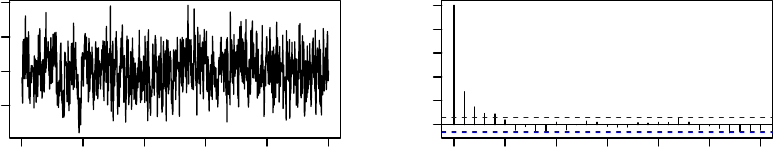
> par(mfrow=c(3,2)) # arrange plots on page in a 3x2 matrix
> plot(mcmcResult$series.worst)
> acf(mcmcResult$series.worst)
These plots, which are shown in Figure 1, suggest that the algorithm approaches station-
arity very quickly, with no appreciable serial dependence beyond lag 5.
Checking the behavior of the worst linear function is a sensible first step in judging
convergence. Our experience with many data examples has shown that this series often
behaves like a worst-case scenario; when the serial dependence in this series has died
down, the dependence in other parameters has also died down. But counterexamples
to this rule do exist, so after examining the worst linear function, it is best to look at
other parameters as well. By default, the mcmcNorm function will save the full series for
all nonredundant model parameters in objects called series.beta and series.sigma.
Each of these is a multivariate time series with rows corresponding to the iterations of
MCMC and columns corresponding to the individual parameters. In the example below,
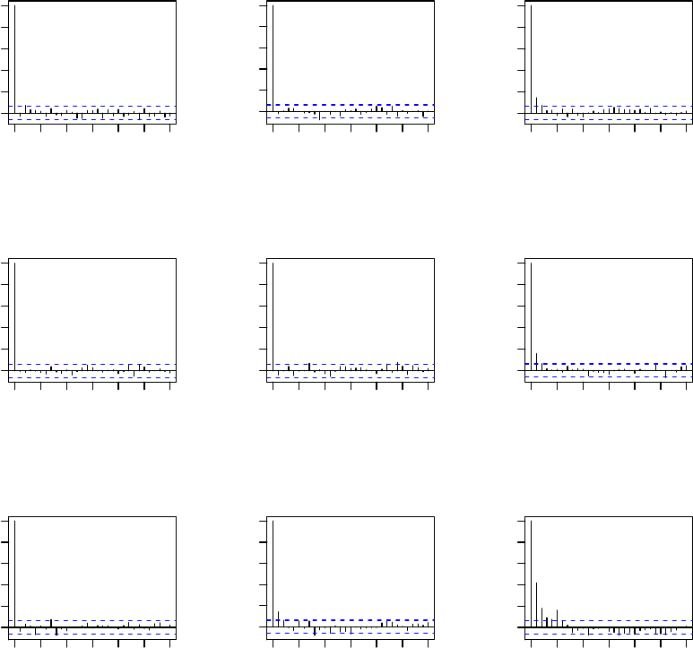
we plot the ACF’s for all parameters, and the resulting plots are displayed in Figure 2.
> dim(mcmcResult$series.beta) # check dimensions of beta series
[1] 1000 3
> dim(mcmcResult$series.sigma) # check dimensions of sigma series
[1] 1000 6
> par(mfrow=c(3,3)) # nine plots per page
> for(i in 1:3)
+ acf(mcmcResult$series.beta[,i],
+ main=colnames(mcmcResult$series.beta)[i])
> for(i in 1:6)
+ acf(mcmcResult$series.sigma[,i],
+ main=colnames(mcmcResult$series.sigma)[i])
6.7 Inferences from simulated parameters
In this data example, it may be of interest to draw inferences about changes in mean
cholesterol over time. Let µj,j= 1,2,3 denote the mean cholesterol levels at the three
occasions, and let δ31 =µ3−µ1be the average change from occasion 1 to occasion 3.
The ML estimate of this parameter is
> emResult$param$beta[1,3] - emResult$param$beta[1,1]
[1] -31.69151
but because EM does not provide measures of uncertainty, we do not know whether this
difference is statistically significant. The parameter series from MCMC, which contain
29
Time
mcmcResult$series.worst
0 200 400 600 800 1000
−0.8 −0.4
0 5 10 15 20 25 30
0.0 0.4 0.8
Lag
ACF
Series mcmcResult$series.worst
Figure 1: Time-series and ACF plots for the worst linear function of the parameters from
1,000 iterations of MCMC applied to the cholesterol data.
simulated draws from their posterior distribution, can be used to compute simulated
Bayesian estimates and intervals for δ31 or any other function of the parameters.
The default number of iterations (iter=1000) used by mcmcNorm is large enough to
diagnose convergence in many problems, but it does not give very accurate estimates of
posterior quantiles. So we will run mcmcNorm for an additional 10,000 iterations, using
the simulated parameters at the end of first run as starting values, and retain only the
parameter series from the new iterations. In effect, the first 1,000 iterations are being
used as a burn-in period.
> mcmcResult <- mcmcNorm(mcmcResult, iter=10000)
Now we simply compute the 10,000 simulated values of δ31 and summarize them.
> delta31 <- mcmcResult$series.beta[,3] -
+ mcmcResult$series.beta[,1]
> mean(delta31) # simulated posterior mean
[1] -31.52694
> quantile(delta31, probs=c(.025,.975) ) # simulated 95% interval
2.5% 97.5%
-57.190033 -5.198703
> table( delta31 < 0 )
FALSE TRUE
108 9892
The simulated 95% Bayesian posterior interval lies entirely below zero, so the drop in
mean cholesterol appears to be statistically significant. About 99% of the simulated
30
0 5 10 15 20 25 30
0.0 0.4 0.8
Lag
ACF
CONST,Y1
0 5 10 15 20 25 30
0.0 0.4 0.8
Lag
ACF
CONST,Y2
0 5 10 15 20 25 30
0.0 0.4 0.8
Lag
ACF
CONST,Y3
0 5 10 15 20 25 30
0.0 0.4 0.8
Lag
ACF
Y1,Y1
0 5 10 15 20 25 30
0.0 0.4 0.8
Lag
ACF
Y2,Y1
0 5 10 15 20 25 30
0.0 0.4 0.8
Lag
ACF
Y3,Y1
0 5 10 15 20 25 30
0.0 0.4 0.8
Lag
ACF
Y2,Y2
0 5 10 15 20 25 30
0.0 0.4 0.8
Lag
ACF
Y3,Y2
0 5 10 15 20 25 30
0.0 0.4 0.8
Lag
ACF
Y3,Y3
Figure 2: ACF plots for all parameters (means and covariances) from 1,000 iterations of
MCMC applied to the cholesterol data.
31
values of δ31 lie below zero, so we are about 99% sure, in the Bayesian sense, that the
average level of cholesterol has declined between occasions 1 and 3.
Simulated parameters from successive iterations of MCMC tend to be positively cor-
related, so these 10,000 values of δ31 carry less information then they would if they were
independent draws from the posterior distribution. If independent draws are needed,
the optional argument multicycle may be helpful. Specifying multicycle=kfor some
k > 1 instructs mcmcNorm to perform the I- and P-step cycle ktimes within each iteration.
Calling mcmcNorm with iter=10000 and multicycle=khas the same effect as running
the algorithm for 10,000 ×kiterations and saving every kth set of simulated parame-
ters. In this example, it is probably conservative to believe that the algorithm achieves
stationarity by 10 cycles, because no significant serial correlations were seen beyond lag
5. Therefore,
> mcmcResult <- mcmcNorm(mcmcResult, iter=10000, multicycle=10)
should produce a beta.series and sigma.series that behave as 10,000 independent
draws from the joint posterior distribution.
6.8 Creating multiple imputations
Another way to use MCMC for inference is to create multiple imputations (MI’s). Simu-
lated values of the missing observations from the I-steps of MCMC can be used as MI’s,
but they need to be independent of one another. The simplest way to achieve indepen-
dence is to save the results from every kth I-step, where kis large enough to ensure
stationarity. We do this by supplying the argument impute.every=kto mcmcNorm. In
the example below, we start at the ML estimate and run the MCMC algorithm for 5,000
iterations, spacing the imputations k= 100 iterations apart to create M= 50 multiple
imputations.
> emResult <- emNorm(cholesterol)
> set.seed(532) # so you can reproduce these results
> mcmcResult <- mcmcNorm(emResult, iter=5000, impute.every=100)
> summary(mcmcResult)
Method: MCMC
Prior: "uniform"
Iterations: 5000
Cycles per iteration: 1
Impute every k iterations, k = 100
No. of imputations created: 50
series.worst present: TRUE
32
series.beta present: TRUE
series.sigma present: TRUE
The result from mcmcNorm now contains an object called imp.list. This is a list with
M= 50 components, where each component is a data matrix that resembles the original
dataset y, except that the missing values have been imputed.
> cholesterol[1:5,] # first 5 rows of original data
Y1 Y2 Y3
1 270 218 156
2 236 234 NA
3 210 214 242
4 142 116 NA
5 280 200 NA
> mcmcResult$imp.list[[1]][1:5,] # first 5 rows of imputed dataset 1
Y1 Y2 Y3
[1,] 270 218 156.0000
[2,] 236 234 179.0431
[3,] 210 214 242.0000
[4,] 142 116 90.7577
[5,] 280 200 185.2721
> mcmcResult$imp.list[[2]][1:5,] # first 5 rows of imputed dataset 2
Y1 Y2 Y3
[1,] 270 218 156.0000
[2,] 236 234 204.7819
[3,] 210 214 242.0000
[4,] 142 116 215.8521
[5,] 280 200 224.6960
The method described above for creating MI’s relies on a single chain of Mk itera-
tions. A slightly different method is to run Mchains of kiterations each. At the end of
each chain, we call the function impNorm to generate a single random imputation based
on the final simulated parameters. In the example below, we run M= 50 chains of 100
iterations each, starting each chain at the ML estimate, generate an imputed dataset at
the end of each chain, and save the imputed datasets as a list.
> imp.list <- as.list(NULL)
> for(m in 1:50){
+ mcmcResult <- mcmcNorm(emResult, iter=100)
+ imp.list[[m]] <- impNorm(mcmcResult) }
33
6.9 Combining the results from post-imputation analyses
Now let’s use the imputed datasets to draw inferences about the mean difference δ31.
With complete data, inferences about this parameter correspond to a paired t-test. That
is, we estimate δ31 by the mean of the difference scores (occasion 3 minus ocasion 1)
among the N= 28 patients. The standard error is the variance of the difference scores
divided by N. In the code below, we generate M= 50 imputed datasets by the single-
chain method, compute the estimate and standard error from each one, and save the
results as two lists.
> emResult <- emNorm(cholesterol)
> set.seed(532) # so you can reproduce these results
> mcmcResult <- mcmcNorm(emResult, iter=5000, impute.every=100)
> est.list <- as.list(NULL) # to hold the estimates
> std.err.list <- as.list(NULL) # to hold the standard errors
> for(m in 1:50){
+ y.imp <- mcmcResult$imp.list[[m]] # one imputed dataset
+ diff <- y.imp[,3] - y.imp[,1] # difference scores
+ est.list[[m]] <- mean(diff)
+ std.err.list[[m]] <- sqrt( var(diff) / length(diff) ) }
Now we combine the results across imputations using the techniques described in Section
4.6, which are implemented in the function miInference. The syntax for calling this
function, as provided in its documentation file, is shown below.
miInference( est.list, std.err.list, method = "scalar",
df.complete = NULL )
Arguments:
est.list: a list of estimates to be combined. Each component of this
list should be a scalar or vector containing point estimates
from the analysis of an imputed dataset. This list should
have _M_ components, where _M_ is the number of imputations,
and all components should have the same length.
std.err.list: a list of standard errors to be combined. Each component
of this list should be a scalar or vector of standard errors
associated with the estimates in ’est.list’.
method: how are the estimates to be combined? At present, the only
type allowed is ’"scalar"’, which means that estimands are
treated as one-dimensional entities. If ’est.list’ contains
vectors, inference for each element of the vector is carried
34
out separately; covariances among them are not considered.
df.complete: degrees of freedom assumed for the complete-data
inference. This should be a scalar or a vector of the same
length as the components of ’est.list’ and ’std.err.list’.
If there were no missing data in this example, tests and intervals for δ31 would be
based on a t-distribution with N−1 = 27 degrees of freedom. Therefore, when we
call miInference, we need to supply the argument df.complete=27.
> miResult <- miInference(est.list, std.err.list, df.complete=27)
> miResult
Est SE Est/SE df p Pct.mis
[1,] -31.84235 11.37477 -2.799383 18.9 0.011 23.3
The overall estimate of −31.8 is close to the ML estimate of −31.7 and the simulated pos-
terior mean of −31.5 reported earlier. The endpoints of the approximate 95% confidence
interval from MI,
> miResult$est - miResult$std.err * qt(.975, miResult$df)
[1] -55.65734
> miResult$est + miResult$std.err * qt(.975, miResult$df)
[1] -8.02737
are also close to the endpoints of the simulated 95% posterior interval (−57.2,−5.20)
reported earlier.
7 Using the package: Example 2
7.1 Marijuana data
We now turn to an example that is less straightforward. Weil, Zinberg, and Nelson (1968)
described an experiment to investigate the effects of marijuana. Nine male subjects
received three treatments each (placebo, low dose and high dose). Under each treatment,
the change in heart rate (beats per minute above baseline) was recorded 15 minutes after
smoking and 90 minutes after smoking, producing six measures per subject, but five of
the 54 data values are missing. These data are distributed with norm2 as a data frame
called marijuana.
35
> data(marijuana)
> marijuana
Plac.15 Low.15 High.15 Plac.90 Low.90 High.90
1 16 20 16 20 -6 -4
2 12 24 12 -6 4 -8
3 8 8 26 -4 4 8
4 20 8 NA NA 20 -4
5 8 4 -8 NA 22 -8
6 10 20 28 -20 -4 -4
7 4 28 24 12 8 18
8 -8 20 24 -3 8 -24
9 NA 20 24 8 12 NA
Classical analysis-of-variance methods for repeated measures make strong assumptions
about the covariance structure. Following the example analyses of Schafer (1997, Chap.
5), we will proceed without assuming any particular form for the within-person covariance
matrix.
7.2 Difficulties with noninformative priors
As in the cholesterol example, we will run the EM algorithm and then use the resulting
ML estimates as starting values for MCMC.
> emResult <- emNorm(marijuana)
Note: Finite-differencing procedure strayed outside
parameter space; solution at or near boundary.
OCCURRED IN: estimate_worst_frac in MOD norm_engine
> set.seed(543)
> mcmcResult <- mcmcNorm(emResult)
Note: Degrees of freedom not positive.
OCCURRED IN: ran_genchi in MOD random_generator
OCCURRED IN: run_pstep in MOD norm_engine
Posterior distribution may not be proper.
MCMC aborted at iteration 1, cycle 1
OCCURRED IN: run_norm_engine_mcmc in MOD norm_engine
What happened? The EM algorithm did converge, but the procedure for estimating
the worst fraction of missing information and worst linear function failed. The warning
message indicates that the EM solution lies at or near the boundary of the parameter
space, meaning that the final estimate of the covariance matrix Σis nearly singular. The
MCMC procedure did not work and aborted at the first cycle. The problem lies with
the prior distribution. The default prior density for Σ, which is prior="uniform", looks
36
like an inverted Wishart density with ξ=−(r+ 1) degrees of freedom, where ris the
number of response variables (Section 3.5). It is not a real density function, however,
because the inverted Wishart density does not exist unless the degrees of freedom exceed
r(Schafer, 1997, Chap. 5). When the sample size is large, this is not a problem, because
the complete-data posterior distribution for Σis inverted Wishart with degrees of freedom
equal ξ+N−p, where ξis the prior degrees of freedom, Nis the sample size, and pis
the number of predictors. But in this particular example, we have r= 6, ξ=−7, N= 9,
and p= 1 (the only predictor is a constant), so the posterior degrees of freedom are
−(r+ 1) + (N−p)=1,
which does not yield a proper posterior distribution even with complete data.
When (N−p) is much larger than r, the choice of prior distribution tends to have
little impact on the results. But with small samples like this one, the uniform prior may
cause difficulty in MCMC. A better choice is the Jeffreys noninformative prior, which
resembles an inverted Wishart density with prior degrees of freedom equal to 0. Under
the Jeffreys prior, the posterior degrees of freedom with complete data are (N−p), which
is proper provided that (N−p)> r.
Let’s see what happens if we run MCMC under the Jeffreys prior starting at the
posterior mode.
> emResult <- emNorm(marijuana, prior="jeffreys")
Note: Finite-differencing procedure strayed outside
parameter space; solution at or near boundary.
OCCURRED IN: estimate_worst_frac in MOD norm_engine
> set.seed(543)
> mcmcResult <- mcmcNorm(emResult)
Note: Matrix not positive definite
OCCURRED IN: cholesky_saxpy in MOD matrix_methods
OCCURRED IN: run_pstep in MOD norm_engine
Posterior distribution may not be proper.
MCMC aborted at iteration 106, cycle 1
OCCURRED IN: run_norm_engine_mcmc in MOD norm_engine
In this run, MCMC aborted at iteration 106. The error message again suggests that the
posterior distribution may not be proper. This time, however, the problem is not that
the degrees of freedom are negative, but that the estimated covariance matrix became
singular or negative definite. This problem arises when the pattern of missing values
causes some aspects of the covariance matrix to be poorly estimated or inestimable from
the observed data.
To get more insight into what is happening, let’s run EM again under a uniform
prior and look at the results.
37
> emResult <- emNorm(marijuana)
> summary(emResult, show.variables=F, show.patterns=F, show.params=F )
Method: EM
Prior: "uniform"
Convergence criterion: 1e-05
Iterations: 288
Converged: TRUE
Max. rel. difference: 8.810968e-06
-2 Loglikelihood: 114.3465
-2 Log-posterior density: 114.3465
Estimated rate of convergence: 0.47868
EM apparently converged, but the estimated covariance matrix is nearly singular, because
its smallest eigenvalue is nearly zero.
> eigen(emResult$param$sigma, symmetric=T, only.values=T)
$values
[1] 7.510111e+02 1.483758e+02 8.574829e+01 4.563068e+01 2.783385e+01
[6] 6.523830e-10
$vectors
NULL
In fact, if we run EM again with a stricter convergence criterion, the procedure aborts,
showing that the ML estimate does indeed lie on the boundary of the parameter space.
> emResult <- emNorm(marijuana, criterion=1e-06)
Note: Attempted logarithm of non-positive number
Cov. matrix became singular or negative definite.
OCCURRED IN: run_estep in MOD norm_engine
EM algorithm aborted at iteration 459
OCCURRED IN: run_norm_engine_em in MOD norm_engine
Warning message:
In emNorm.default(marijuana, criterion = 1e-06) :
Algorithm did not converge by iteration 464
7.3 Using a ridge prior
When aspects of the covariance structure are poorly estimated or inestimable, one remedy
is to introduce a small amount or prior information. The ridge prior (Section 3.5),
allows the variances to be estimated from the observed data, but smooths the estimated
38
Time
mcmcResult$series.worst
0 1000 2000 3000 4000 5000
−0.8 −0.4 0.0
0 5 10 15 20 25 30 35
0.0 0.4 0.8
Lag
ACF
Series mcmcResult$series.worst
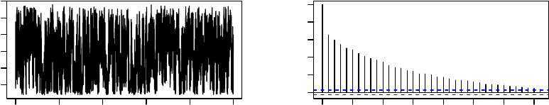
Figure 3: Time-series and ACF plots for the worst linear function of the parameters from
5,000 iterations of MCMC applied to the marijauna data under ridge prior.
correlations toward zero. The degree of smoothing is controlled by the prior degrees of
freedom ξ, which is specified via the argument prior.df. In many cases, we can stabilize
the inference with very small amounts of prior information. Here we apply a ridge prior
with ξ= 0.5 and run 5,000 iterations of MCMC starting from the posterior mode.
> emResult <- emNorm(marijuana, prior="ridge", prior.df=0.5)
> set.seed(543)
> mcmcResult <- mcmcNorm(emResult, iter=5000)
This time, the procedure ran without difficulty. Plots of the worst linear function (Figure
3) show that MCMC converges slowly because the rates of missing information are high.
7.4 Inferences by parameter simulation
The slow convergence of MCMC in this example indicates that many iterations will be
required to get precise estimates for quantities of interest. Here we perform an analysis
similar to that of Schafer (1997, Sec. 5.4), examining posterior distributions for contrasts
among the means of the repeated measurements. Let µj,j= 1, . . . , 6 denote the means
for the six measurements, and let δjk =µj−µkdenote a contrast between two means.
In the code below, we run 10,000 iterations of MCMC, cycling the procedure 100 times
within each iteration, so that the simulated draws saved to the parameter series are
approximately independent. From the series, we compute 10,000 simulated values for
the six contrasts δ21,δ31,δ32,δ54,δ64, and δ65, and summarize them with a boxplot-like
graph that, except for a minor amount of random noise, replicates the results shown in
Schafer (1997, Fig. 5.9). The boxplot-like graph is shown in Figure 4.
> set.seed(876)
39
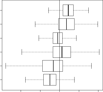
d65 d64 d54 d32 d31 d21
−40 −20 0 20 40
Figure 4: Simulated posterior medians, quartiles and 95% equal-tailed posterior intervals
for six contrasts from the marijuana dataset.
> mcmcResult <- mcmcNorm(emResult, iter=10000, multicycle=100)
>
> diff.scores <- cbind(
+ d65 = mcmcResult$series.beta[,6] - mcmcResult$series.beta[,5],
+ d64 = mcmcResult$series.beta[,6] - mcmcResult$series.beta[,4],
+ d54 = mcmcResult$series.beta[,5] - mcmcResult$series.beta[,4],
+ d32 = mcmcResult$series.beta[,3] - mcmcResult$series.beta[,2],
+ d31 = mcmcResult$series.beta[,3] - mcmcResult$series.beta[,1],
+ d21 = mcmcResult$series.beta[,2] - mcmcResult$series.beta[,1] )
>
> # construct boxplot-like graph showing the posterior
> # median, quartiles and 95% interval for each contrast
> stats <- matrix( NA, 5, 6)
> for(i in 1:6)
+ stats[,i] <- quantile( diff.scores[,i], probs=c(.025,.25,.5,.75,.975))
> box.stats <- list( stats=stats, names=colnames(diff.scores) )
> bxp( box.stats, horizontal=T )
> abline(v=0)
40
8 Using the package: Example 3
8.1 FLAS data
Our third example uses the dataset flas. These data come from a pilot study to assess
the reliability and validity of the Foreign Language Attitude Scale (FLAS), an instrument
for predicting success in the study or foreign languages (Raymond and Roberts, 1983).
The questionnaire was given to N= 279 students enrolled in four different language
courses (French, German, Spanish, Russian) at Penn State University. This dataset
includes FLAS score, final grade in the course, and other variables relevant to academic
achievement. The variables in the dataset, as shown in its documentation file, are:
’LAN2’ 1=Spanish, 0=other.
’LAN3’ 1=German, 0=other.
’LAN4’ 1=Russian, 0=other.
’AGE’ age group (1=less than 20, 2=20+).
’PRI’ number of prior foreign language courses (1=none, 2=1-2,
3=3+).
’SEX’ 0=male, 1=female
’MLAT’ Modern Language Aptitude Test
’FLAS’ Foreign Language Attitude Scale
’SATV’ Scholastic Aptitude Test, verbal score
’SATM’ Scholastic Aptitude Test, math score
’ENG’ score on Penn State English placement exam
’HGPA’ high school grade point average
’CGPA’ current college grade point average
’GRD’ final grade in foreign language course (1=B or lower, 2=A)
Notice that the language variable, a nominal variable with four categories and no missing
values, has been converted to three dummy codes. Including these dummy codes either as
41
responses or predictors allows the means of the other variables to vary without constraints
across the four language groups.
8.2 Applying a ridge prior
When the EM algorithm is applied to the FLAS dataset, it converges quickly.
> data(flas)
> emResult <- emNorm(flas)
Note: Eigen power method failed to converge.
OCCURRED IN: estimate_worst_frac in MOD norm_engine
> summary(emResult, show.variables=F, show.patterns=F, show.params=F)
Method: EM
Prior: "uniform"
Convergence criterion: 1e-05
Iterations: 17
Converged: TRUE
Max. rel. difference: 6.0021e-06
-2 Loglikelihood: 7310.107
-2 Log-posterior density: 7310.107
Worst fraction missing information: NA
The quick convergence of EM suggests that the rates of missing information are low.
However, the procedure for estimating the worst fraction of missing information failed,
suggesting that something has gone awry. If we try to run MCMC using the default
uniform prior, we encounter difficulty. The procedure does not abort, but the time-series
and ACF plots for the mean of the variable GRD, which are shown in Figure 5, show that
this parameter exhibits long-term drift. (In this example, the worst linear function of the
parameters is not available, so we need to diagnose convergence by examine time-series
and ACF plots for individual elements or other functions of βand Σ.)
> set.seed(765)
> mcmcResult <- mcmcNorm(emResult)
> par(mfrow=c(3,2))
> plot(mcmcResult$series.beta[,14])
> acf( mcmcResult$series.beta[,14])
Long-term drifts in a parameter series suggest that the parameter is poorly estimated
or inestimable. Estimability problems may arise when missing values fall in a malicious
pattern. In this example, the problem is that value of GRD happens to be missing for
everyone who studied Russian.
42
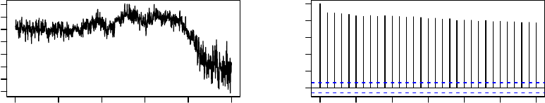
Time
mcmcResult$series.beta[, 14]
0 200 400 600 800 1000
1.0 1.2 1.4 1.6
0 5 10 15 20 25 30
0.0 0.4 0.8
Lag
ACF
Series mcmcResult$series.beta[, 14]
Figure 5: Time-series and ACF plots for the mean of variable GRD from 1,000 iterations
of MCMC applied to the FLAS data under a uniform prior.
> table( flas$LAN4, is.na(flas$GRD))
FALSE TRUE
0 232 27
1 0 20
This pattern of missing values makes it impossible to estimate the mean of GRD among
those who study Russian. With an improper prior distribution and a malicious pattern of
missing values, it is possible to have a situation where, even though the I- and P-steps are
well defined at each iteration, the posterior distribution does not exist, and the MCMC
algorithm cannot converge (Schafer, 1997, Sec. 3.5).
When some parameters are inestimable, different starting values for EM may lead
to different parameter estimates with exactly the same loglikelihood. We can diagnose
inestimability using a combination of EM and MCMC. In the code example below, we
use MCMC to generate random starting values for the parameters and then run EM
from these random starts. The three EM runs converge to different solutions (note the
different estimates for the mean of GRD), but the loglikelihood at the three solutions looks
exactly the same.
> data(flas)
> emResult <- emNorm(flas)
Note: Eigen power method failed to converge.
OCCURRED IN: estimate_worst_frac in MOD norm_engine
> summary(emResult, show.variables=F,
+ show.patterns=F, show.params=F)
Method: EM
Prior: "uniform"
43
Convergence criterion: 1e-05
Iterations: 17
Converged: TRUE
Max. rel. difference: 6.0021e-06
-2 Loglikelihood: 7310.107
-2 Log-posterior density: 7310.107
Worst fraction missing information: NA
Eigen power method failed to converge.
OCCURRED IN: estimate_worst_frac in MOD norm_engine
> set.seed(765)
> mcmcResult <- mcmcNorm(emResult)
> par(mfrow=c(3,2))
> plot(mcmcResult$series.beta[,14])
> acf( mcmcResult$series.beta[,14])
> # generate three random starts by running MCMC
> # from the EM estimates
> set.seed(321)
> random.start.1 <- mcmcNorm(emResult,iter=100)
> random.start.2 <- mcmcNorm(emResult,iter=100)
> random.start.3 <- mcmcNorm(emResult,iter=100)
> # now run EM from the random starts
> emResult.1 <- emNorm( random.start.1 )
> emResult.2 <- emNorm( random.start.2 )
> emResult.3 <- emNorm( random.start.3 )
> # compare the loglikelihoods at the three EM solutions
> loglikNorm( emResult.1 )
[1] -3655.054
> loglikNorm( emResult.2 )
[1] -3655.054
> loglikNorm( emResult.3 )
[1] -3655.054
> # compare the estimates of beta
> emResult.1$param$beta
LAN2 LAN3 LAN4 AGE PRI
CONST 0.2795699 0.4086022 0.07168459 1.530772 2.196905
SEX MLAT FLAS SATV SATM
CONST 0.4527892 82.48746 24.11213 498.3939 560.6742
ENG HGPA CGPA GRD
CONST 52.85448 2.749734 3.265421 1.39928
44
> emResult.2$param$beta
LAN2 LAN3 LAN4 AGE PRI
CONST 0.2795699 0.4086022 0.07168459 1.530772 2.196905
SEX MLAT FLAS SATV SATM
CONST 0.4527892 82.48746 24.11213 498.3939 560.6742
ENG HGPA CGPA GRD
CONST 52.85448 2.749734 3.265421 1.537627
> emResult.3$param$beta
LAN2 LAN3 LAN4 AGE PRI
CONST 0.2795699 0.4086022 0.07168459 1.530772 2.196905
SEX MLAT FLAS SATV SATM
CONST 0.4527892 82.48746 24.11213 498.3939 560.6742
ENG HGPA CGPA GRD
CONST 52.85448 2.749734 3.265421 1.728877
8.3 Applying a ridge prior
To overcome the problem of inestimability, we apply a ridge prior with ξ= 3 prior degrees
of freedom. This small amount of information, which corresponds to about 1% of the
sample size, is enough to identify the inestimable parameters. With this prior, MCMC
does converge, but very slowly. Here we run MCMC from 100,000 iterations beginning
from the posterior mode, and then we plot the time series and ACF for the mean of GRD.
The plots are shown in Figure 6.
> emResult <- emNorm(flas, prior="ridge", prior.df=3)
> set.seed(765)
> # relax, this may take a little while
> mcmcResult <- mcmcNorm(emResult, iter=100000)
> par(mfrow=c(2,2))
> # plot first tenth of the series
> plot(mcmcResult$series.beta[1:10000,14],type="l")
> # estimate the acf from the whole series
> acf( mcmcResult$series.beta[,14], lag.max=600, col="grey")
(If you are unable to run this example because of the memory limitations of your system,
try reducing the number of iterations to iter=1000 and use the option multicycle=100.
MCMC will still run for 100,000 cycles, but mcmcNorm will save the simulated parameters
only at every 100th cycle, and the ACF will die down by lag 6 rather than lag 600.)
45
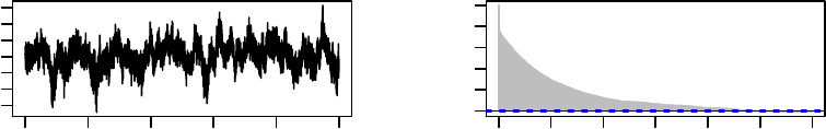
0 2000 4000 6000 8000 10000
1.2 1.5 1.8
Index
mcmcResult$series.beta[1:10000, 14]
0 100 200 300 400 500 600
0.0 0.4 0.8
Lag
ACF
Series mcmcResult$series.beta[, 14]
Figure 6: Time-series and ACF plots for the mean of variable GRD from MCMC applied
to the FLAS data under a ridge prior.
8.4 Analysis by multiple imputation
In earlier analyses of these data, Schafer (1997, Sec. 6.3) imputed missing values under the
joint normal model and then analyzed the imputed data by fitting logistic regressions
with GRD as a binary response. Now we will try to replicate those results. First, we
run MCMC for 50,000 iterations using a ridge prior with ξ= 3. We save the imputed
values at every 1,000th iteration, producing M= 50 multiple imputations. Because we
no longer need to save the parameter series, we now call mcmcNorm with the argument
save.all.series=FALSE.
> emResult <- emNorm(flas, prior="ridge", prior.df=3)
> set.seed(765)
> mcmcResult <- mcmcNorm(emResult, iter=50000,
+ save.all.series=FALSE, impute.every=1000)
After imputation, we round off the imputed values for the discrete variables AGE,PRI,SEX
and GRD to the nearest categories. Then we recode AGE to a dummy indicator for age ≥
20 and characterize the effect of PRI with linear and quadratic terms. Finally, we regress
an indicator for GRD=2 on the entire set of recoded covariates, saving the coefficients and
standard errors, and combine the results by Rubin’s (1987) rules for scalar estimands.
> est.list <- as.list(NULL) # to hold estimated coefficients
> std.err.list <- as.list(NULL) # to hold their standard errors
> for(m in 1:50){
+ imp <- mcmcResult$imp.list[[m]] # one imputed datasset
+ imp <- data.frame(imp) # convert into a data frame
+ # round AGE and change to dummy indicator for age=20+
+ imp$AGE.2 <- 1*(imp$AGE>1.5) # dummy indicator for age=20+
+ # round PRI and define linear, quadratic terms
46
+ imp$PRI <- round(imp$PRI)
+ imp$PRI[imp$PRI<1] <- 1
+ imp$PRI[imp$PRI>3] <- 3
+ imp$PRI.L <- -1*(imp$PRI==1) +0*(imp$PRI==2) + 1*(imp$PRI==3)
+ imp$PRI.Q <- 1*(imp$PRI==1) -2*(imp$PRI==2) + 1*(imp$PRI==3)
+ # round SEX and change to dummy indicator for female
+ imp$SEX <- 1*(imp$SEX>.5)
+ # round imputed GRD and recode to 1=A, 0=B or lower
+ imp$GRD <- 1*(imp$GRD > 1.5)
+ # fit logistic model
+ glmResult <- glm( GRD ~ LAN2 + LAN3 + LAN4 + AGE.2 + PRI.L +
+ PRI.Q + SEX + MLAT + FLAS + SATV + SATM + ENG + HGPA + CGPA,
+ data=imp, family=binomial)
+ # save estimates and SE’s
+ est.list[[m]] <- glmResult$coefficients
+ std.err.list[[m]] <-
+ sqrt( diag( summary(glmResult)$cov.scaled ) ) }
> # combine the results by Rubin’s (1987) rules
> miResult <- miInference(est.list, std.err.list)
> miResult
Est SE Est/SE df p
(Intercept) -1.5495e+01 2.9395e+00 -5.271 810.5 0.000
LAN2 3.6052e-01 5.0760e-01 0.710 2484.9 0.478
LAN3 1.1272e+00 4.4173e-01 2.552 7161.6 0.011
LAN4 -2.1253e-01 6.6213e+02 0.000 527837921.7 1.000
AGE.2 1.3719e+00 4.4020e-01 3.117 1014.3 0.002
PRI.L 2.9659e-01 2.4933e-01 1.190 1198.9 0.234
PRI.Q -1.3100e-01 1.4701e-01 -0.891 1267.0 0.373
SEX 7.5617e-01 4.4557e-01 1.697 1272.6 0.090
MLAT 4.0815e-02 1.5886e-02 2.569 789.4 0.010
FLAS 1.0839e-01 5.0364e-02 2.152 366.9 0.032
SATV -3.3027e-03 3.3211e-03 -0.994 1018.8 0.320
SATM 2.9059e-04 2.6788e-03 0.108 1975.8 0.914
ENG 9.5108e-03 2.2439e-02 0.424 919.0 0.672
HGPA 2.2366e+00 4.5447e-01 4.921 1678.3 0.000
CGPA 8.5284e-01 5.4255e-01 1.572 697.9 0.116
Pct.mis
(Intercept) 24.6
LAN2 14.0
LAN3 8.3
LAN4 0.0
AGE.2 22.0
PRI.L 20.2
PRI.Q 19.7
47
SEX 19.6
MLAT 24.9
FLAS 36.5
SATV 21.9
SATM 15.7
ENG 23.1
HGPA 17.1
CGPA 26.5
The results from this analysis are quite similar to those reported by Schafer (1997, Table
6.8). The differences could plausibly be due to random noise, except for one discrepancy:
the standard error for the coefficient of LAN4 shown above is huge. This is the one param-
eter for which the observed data carry essentially no information. The logistic regression
procedure converged for all M= 50 imputed datasets, but for some of these, the esti-
mated standard error was very large, suggesting that the Hessian of the loglikelihood was
nearly singular. These large standard errors inflated the value of the within-imputation
variance ¯
Uand caused the estimated rate of missing information for this parameter to
be essentially zero.
9 References
Barnard, J. and Rubin, D.B. (1999) Small-sample degrees of freedom with multiple im-
putation. Biometrika, 86, 948–955.
Bernaards, C.A., Belin, T.R. and Schafer, J.L. (2007) Robustness of a multivariate normal
approximation for imputation of incomplete binary data. Statistics in Medicine, 26,
1368–1382.
Fraley, C. (1998) On Computing the Largest Fraction of Missing Information for the EM
Algorithm and the Worst Linear Function for Data Augmentation. Technical Report No.
332, Department of Statistics, University of Washington, Seattle.
Goodnight, J.H. (1979) A tutorial on the SWEEP operator. The American Statistician,
33, 149–158.
Little, R.J.A. and Rubin, D.B. (2002) Statistical Analysis with Missing Data (2nd Ed.).
New York: Wiley.
Meng, X.-L. and Rubin, D.B. (1994) On the global and componentwise rates of conver-
gence of the EM algorithm. Linear Algebra and its Applications, 199 (Supplement 1),
413–425.
Raymond, M.R. and Roberts, D.M. (1983) Development and validation of a foreign
48
language attitude scale. Educational and Psychological Measurement, 43, 1239–1246.
Rubin, D.B. (1974) Characterizing the estimation of parameters in incomplete data prob-
lems. Journal of the American Statistical Association, 69, 467–474.
Rubin, D.B. (1976) Inference and missing data. Biometrika, 63, 581–592.
Rubin, D.B. (1987) Multiple Imputation for Nonresponse in Surveys. New York: Wiley.
Ryan, B.F. and Joiner, B.L. (1994) Minitab Handbook (Third edition). Belmont, CA:
Wadsworth.
Schafer, J.L. (1997) Analysis of Incomplete Multivariate Data. London: Chapman &
Hall.
Weil, A.T., Zinberg, N.E. and Nelson, J.M. (1968) Clinical and psychological effects of
marihuana in man. Science, 162, 1234–1242.
49
