Operators Manual Izod
User Manual:
Open the PDF directly: View PDF ![]() .
.
Page Count: 67
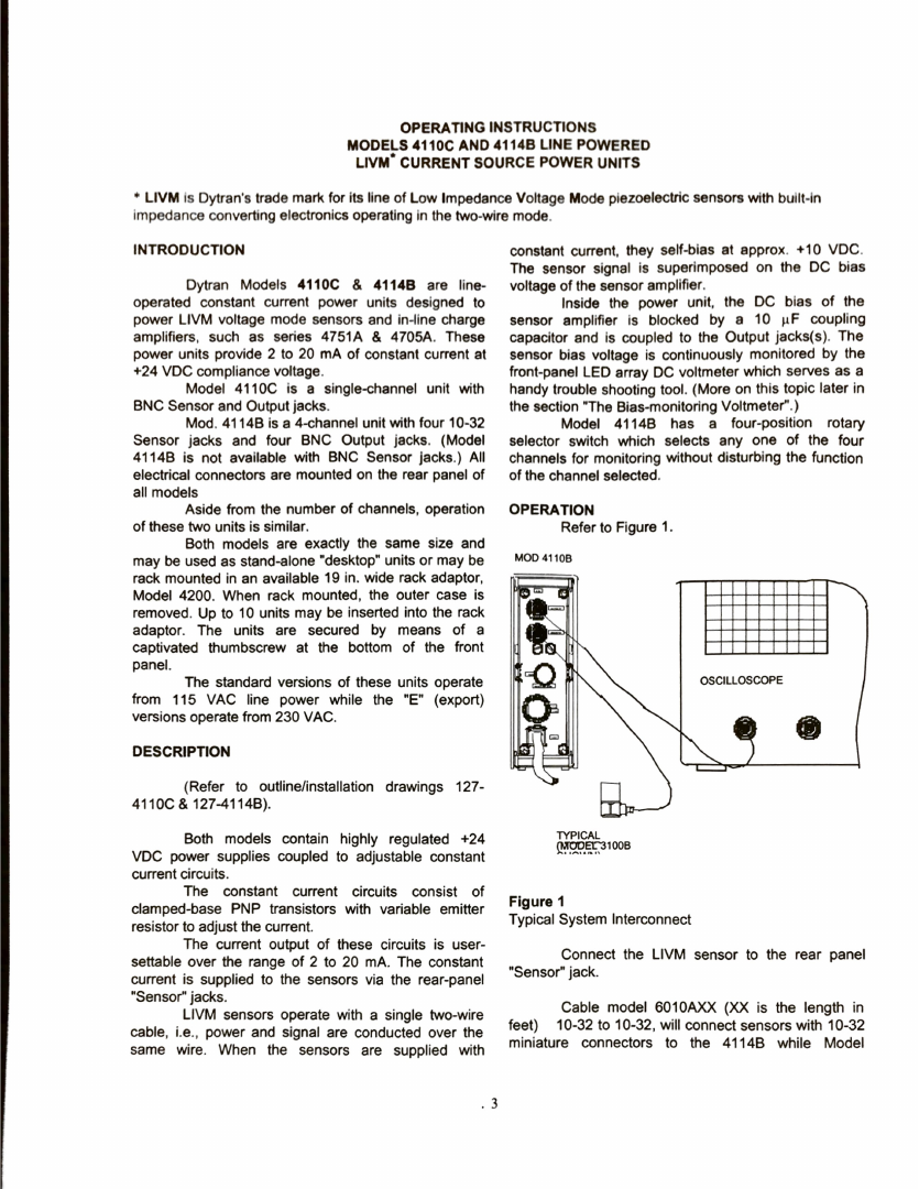
- Operation Instructions
- Troubleshooting
- Electrical Components
- ASTM Methodologies

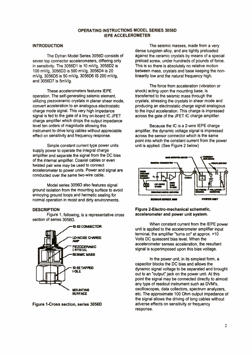
OPERATOR’S MANUAL - IZOD MACHINE
Prepared by: 2018 - MNE 520 - Dr. Guven
Impact Test Setup to Measure Fracture Toughness of Materials
Abdullah Almarri
Arnaud Debraine
Gregory Nelson
Stephanie Fulenwider
Senior Design - Capstone Project
May 7, 2018
CONTENTS
Contents
1 Operation Instructions 4
1.1 Install Software on New Computer . . . . . . . . . . . . . . . . . . . . . . . . . . . 4
1.1.1 Install Anaconda on Windows . . . . . . . . . . . . . . . . . . . . . . . . . 4
1.1.2 Import Arduino Environment . . . . . . . . . . . . . . . . . . . . . . . . . . 5
1.2 Start Software . . . . . . . . . . . . . . . . . . . . . . . . . . . . . . . . . . . . . . . 6
1.2.1 On Windows Using Anaconda Prompt . . . . . . . . . . . . . . . . . . . . . 6
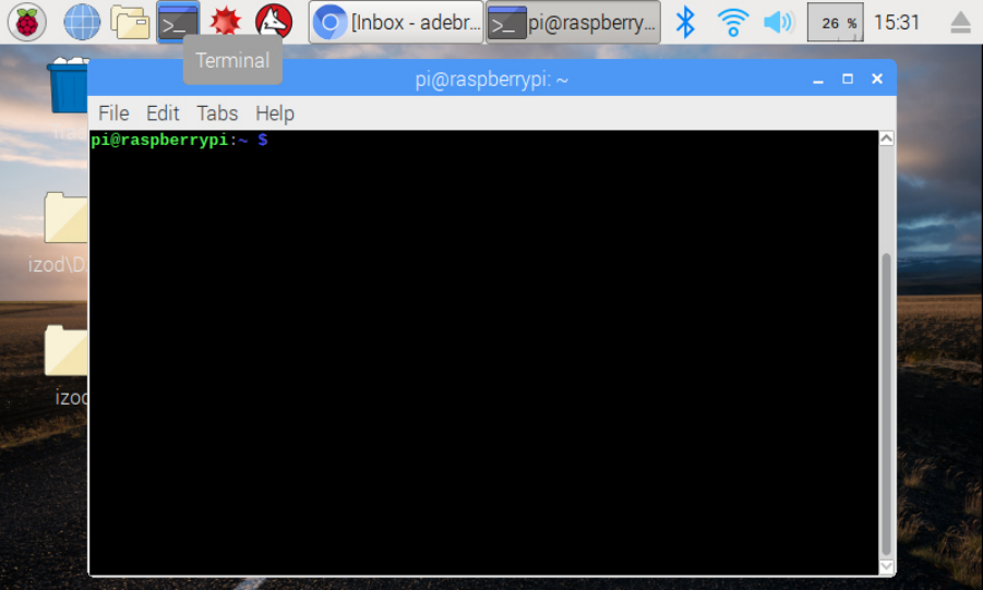
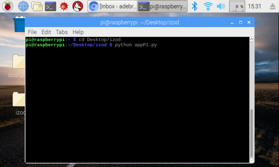
1.2.2 On Raspbian Using Terminal . . . . . . . . . . . . . . . . . . . . . . . . . . 9
1.3 Find Zero Position . . . . . . . . . . . . . . . . . . . . . . . . . . . . . . . . . . . . 11
1.4 Load a Specimen . . . . . . . . . . . . . . . . . . . . . . . . . . . . . . . . . . . . . 12
1.5 Perform a Test . . . . . . . . . . . . . . . . . . . . . . . . . . . . . . . . . . . . . . . 13
1.6 Reset Arm Position . . . . . . . . . . . . . . . . . . . . . . . . . . . . . . . . . . . . 14
1.7 Software Interface Details . . . . . . . . . . . . . . . . . . . . . . . . . . . . . . . . 15
1.7.1 Windows Desktop Version . . . . . . . . . . . . . . . . . . . . . . . . . . . . 15
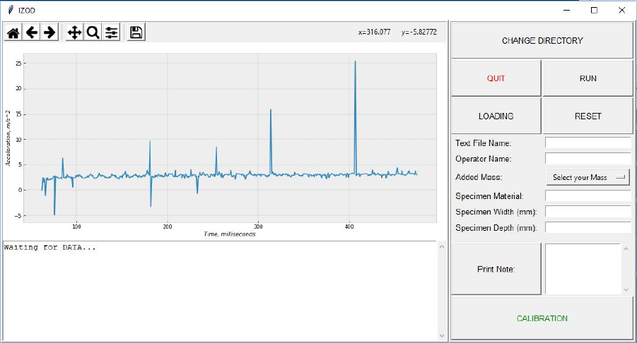
1.7.2 Raspbian Touchscreen Version . . . . . . . . . . . . . . . . . . . . . . . . . 18
1.8 Text File Output Details . . . . . . . . . . . . . . . . . . . . . . . . . . . . . . . . . 19
2 Troubleshooting 20
2.1 Swap Computer/Touchscreen . . . . . . . . . . . . . . . . . . . . . . . . . . . . . 20
2.2 Swap Weights . . . . . . . . . . . . . . . . . . . . . . . . . . . . . . . . . . . . . . . 21
2.3 Invert Touchscreen Display . . . . . . . . . . . . . . . . . . . . . . . . . . . . . . . 22
2.4 Incorrect Arm Starting Position . . . . . . . . . . . . . . . . . . . . . . . . . . . . . 24
2.4.1 Arm Before ZERO Position . . . . . . . . . . . . . . . . . . . . . . . . . . . . 24
2.4.2 Arm After ZERO Position . . . . . . . . . . . . . . . . . . . . . . . . . . . . . 25
2.5 Unresponsive Software Buttons/Arduino Communication Malfunction . . . . . 26
2.6 Bypass Software Interface . . . . . . . . . . . . . . . . . . . . . . . . . . . . . . . . 27
2.7 Reset File Count to Default . . . . . . . . . . . . . . . . . . . . . . . . . . . . . . . 28
2.8 Modify Constants (Weight, Arm Length, etc...) . . . . . . . . . . . . . . . . . . . . 29
May 7, 2018 1 of 66
CONTENTS
2.9 Anaconda Starter Guide . . . . . . . . . . . . . . . . . . . . . . . . . . . . . . . . . 30
2.10 Conda Cheat Sheet . . . . . . . . . . . . . . . . . . . . . . . . . . . . . . . . . . . . 32
3 Electrical Components 34
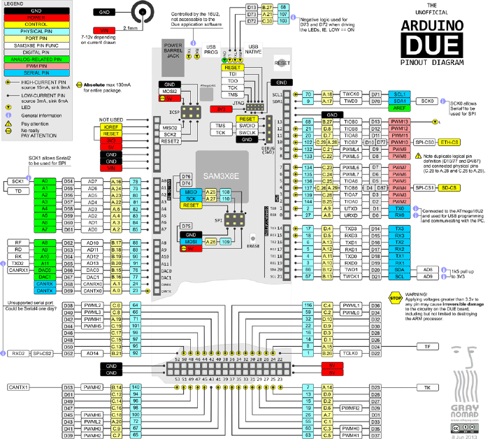
3.1 Arduino DUE . . . . . . . . . . . . . . . . . . . . . . . . . . . . . . . . . . . . . . . 34
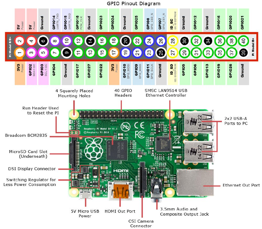
3.2 Raspberry Pi 3 . . . . . . . . . . . . . . . . . . . . . . . . . . . . . . . . . . . . . . . 35
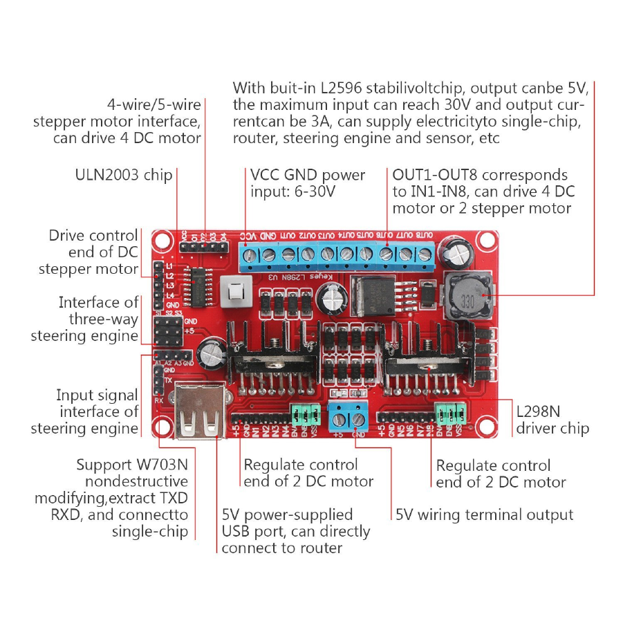
3.3 L298N V3 Motor Controller . . . . . . . . . . . . . . . . . . . . . . . . . . . . . . . 36
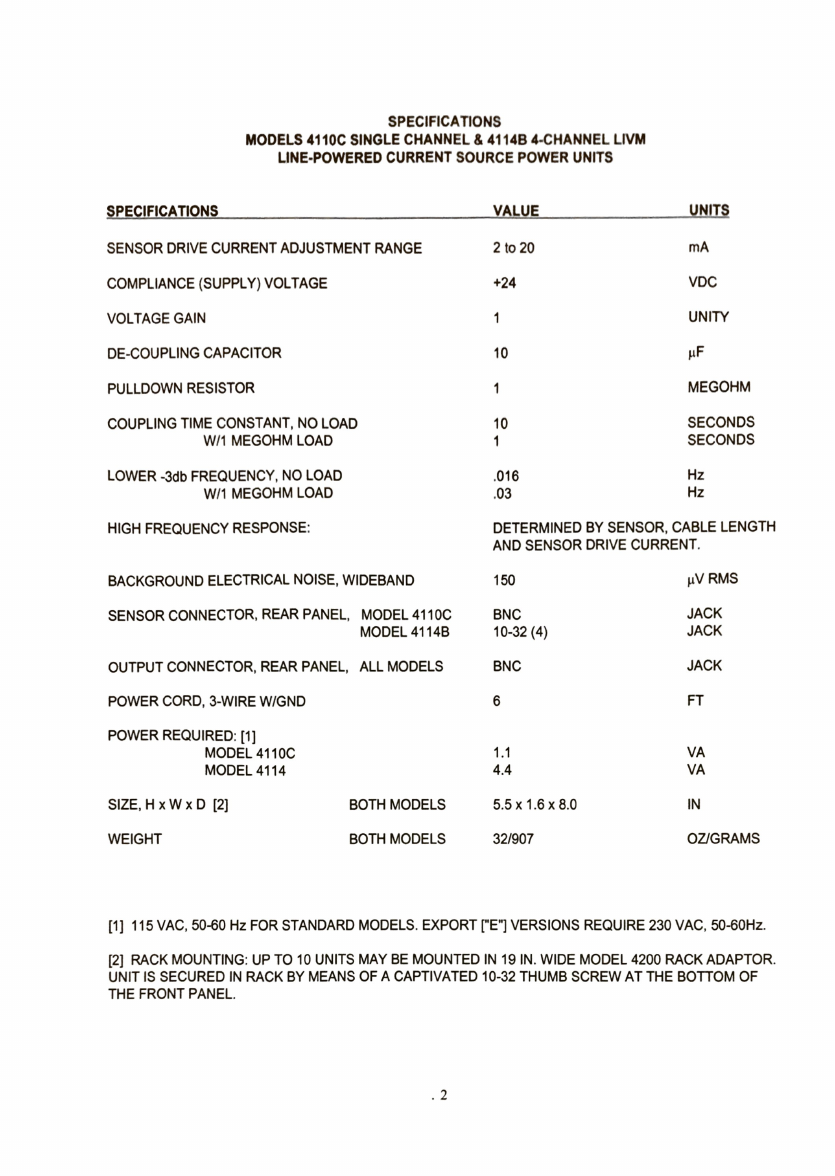
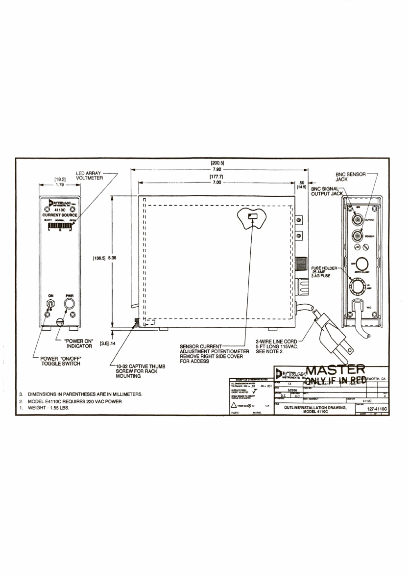
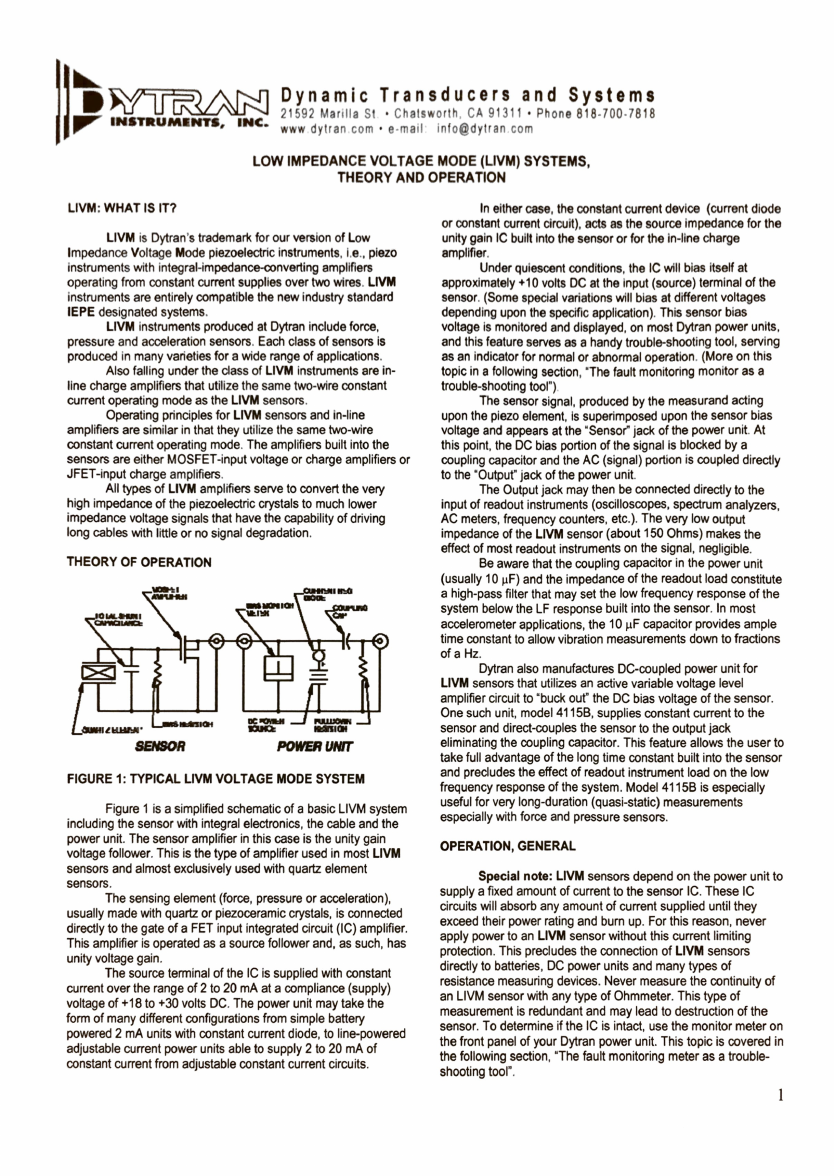
3.4 Dytran 4110C Current Source . . . . . . . . . . . . . . . . . . . . . . . . . . . . . . 37
3.5 NEMA17 100:1 Stepper Motor . . . . . . . . . . . . . . . . . . . . . . . . . . . . . . 47
3.6 Encoder . . . . . . . . . . . . . . . . . . . . . . . . . . . . . . . . . . . . . . . . . . . 49
3.7 Electro-Magnet . . . . . . . . . . . . . . . . . . . . . . . . . . . . . . . . . . . . . . 51
3.8 Dytran Accelerometers . . . . . . . . . . . . . . . . . . . . . . . . . . . . . . . . . . 52
3.8.1 General Accelerometer Specifications . . . . . . . . . . . . . . . . . . . . . 52
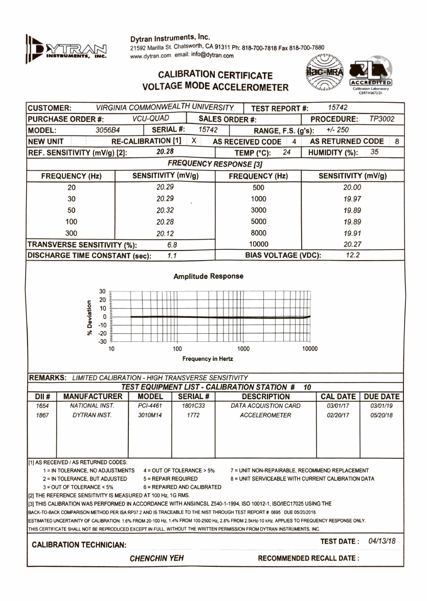
3.8.2 3056B4-15742 . . . . . . . . . . . . . . . . . . . . . . . . . . . . . . . . . . . 57
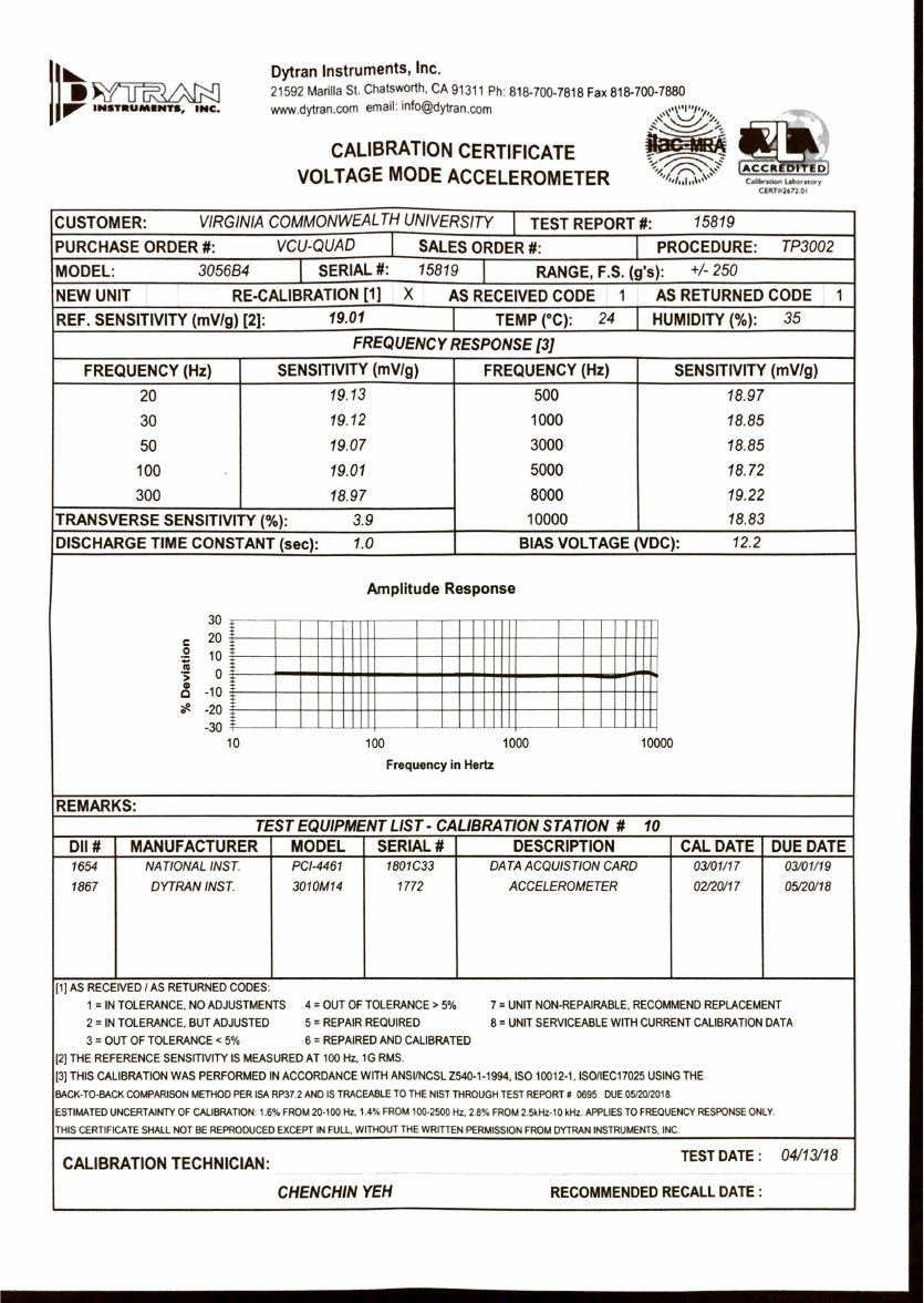
3.8.3 3056B4-15819 . . . . . . . . . . . . . . . . . . . . . . . . . . . . . . . . . . . 58
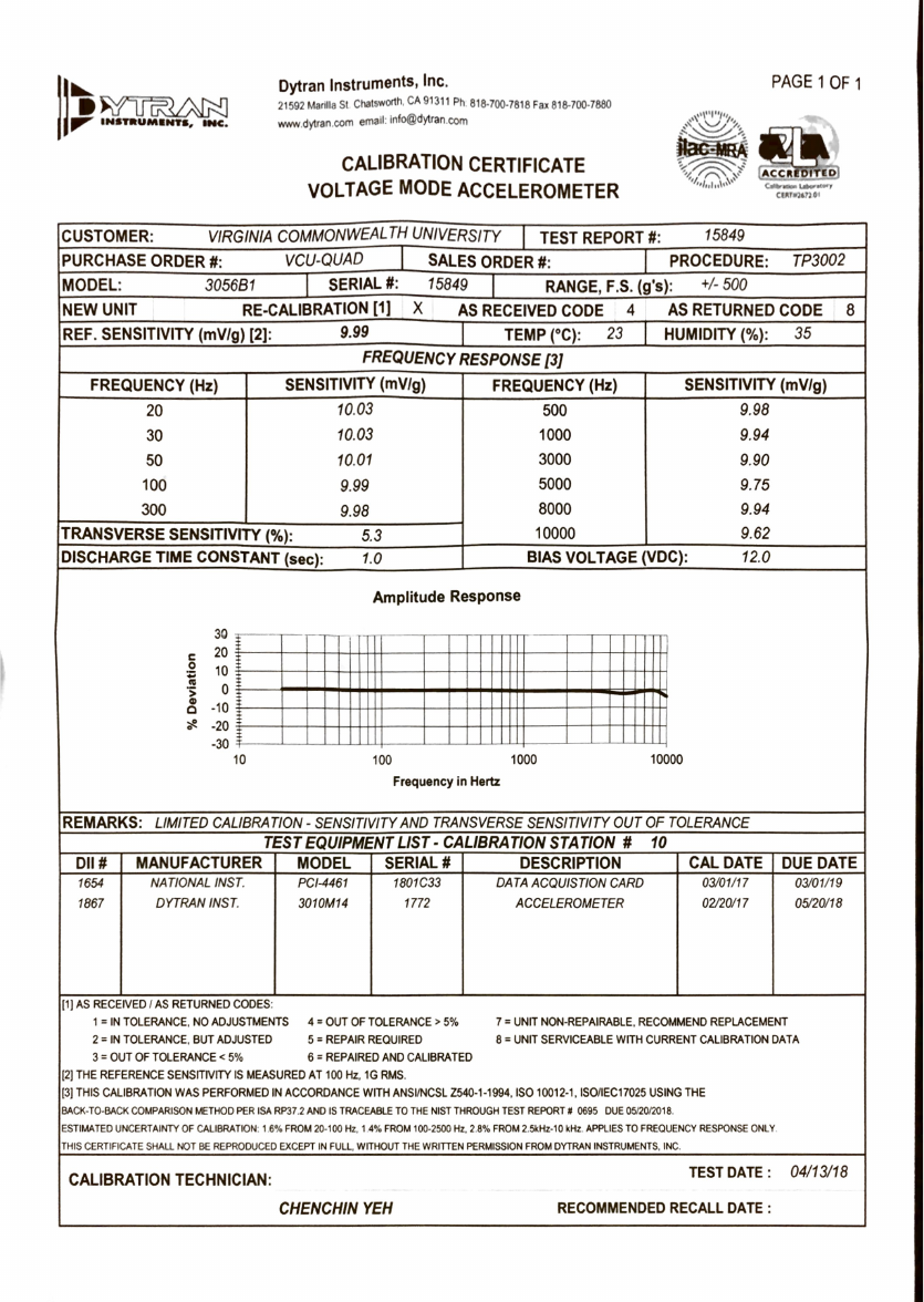
3.8.4 3056B1-15849 . . . . . . . . . . . . . . . . . . . . . . . . . . . . . . . . . . . 59
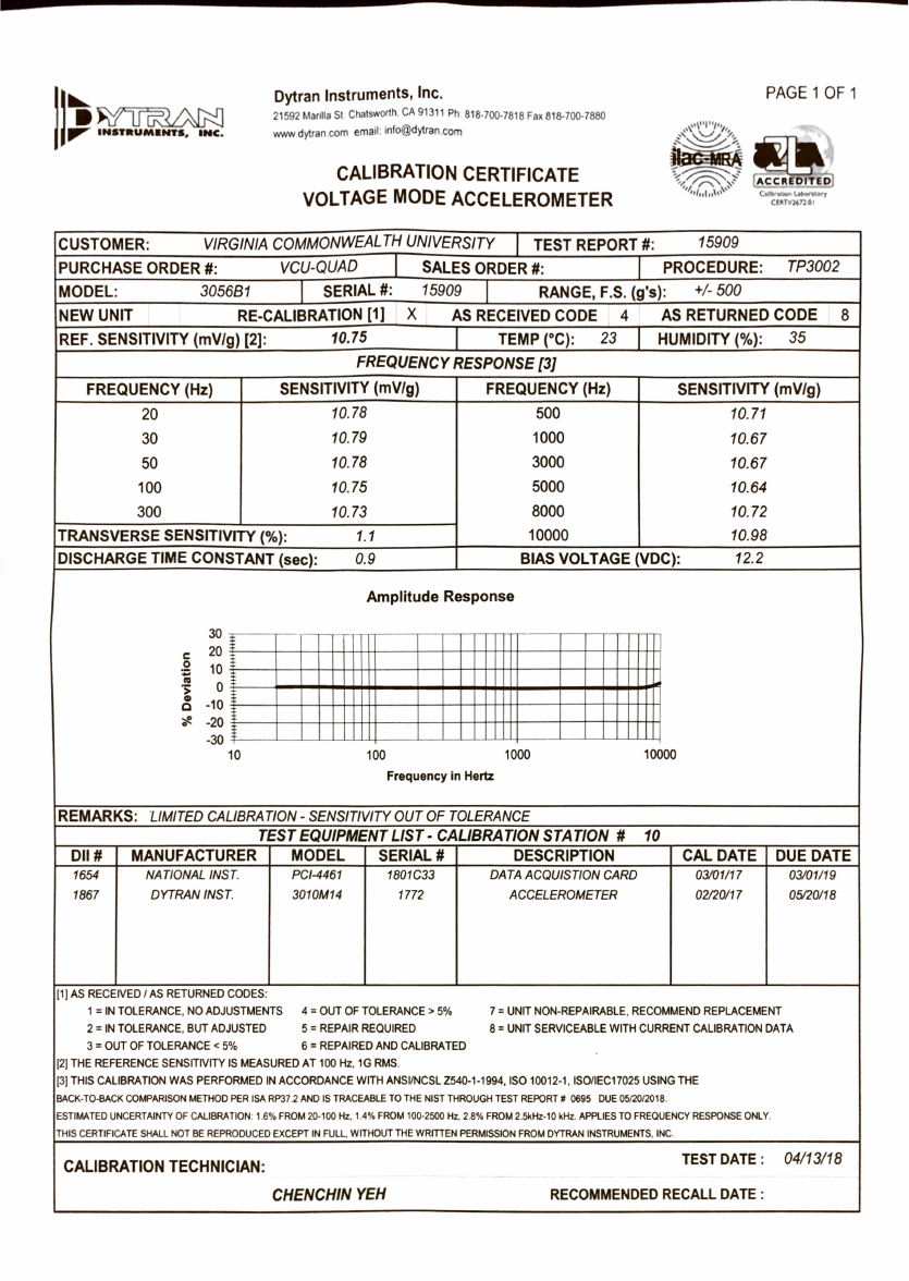
3.8.5 3056B1-15909 . . . . . . . . . . . . . . . . . . . . . . . . . . . . . . . . . . . 60
3.8.6 3056D4-18611 . . . . . . . . . . . . . . . . . . . . . . . . . . . . . . . . . . . 61
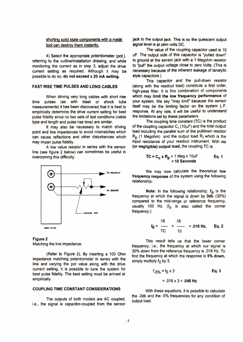
3.9 Wiring/Electrical Circuit . . . . . . . . . . . . . . . . . . . . . . . . . . . . . . . . . 62
4 ASTM Methodologies 63
4.1 Measuring Effective Weight of the Hammer . . . . . . . . . . . . . . . . . . . . . . 63
4.2 Measuring Effective Length of the Hammer . . . . . . . . . . . . . . . . . . . . . . 64
4.3 Specimen Failure Types . . . . . . . . . . . . . . . . . . . . . . . . . . . . . . . . . 65
4.4 Specimen Dimensions for IZOD-type test . . . . . . . . . . . . . . . . . . . . . . . 66
May 7, 2018 2 of 66
LIST OF FIGURES
List of Figures
1.1 Install Arduino Environment . . . . . . . . . . . . . . . . . . . . . . . . . . . . . . 5
1.2 Start Spyder Using Anaconda Prompt . . . . . . . . . . . . . . . . . . . . . . . . . 6
1.3 Start Software from Spyder . . . . . . . . . . . . . . . . . . . . . . . . . . . . . . . 7
1.4 Start Software from Anaconda Prompt . . . . . . . . . . . . . . . . . . . . . . . . . 8
1.5 Open Terminal . . . . . . . . . . . . . . . . . . . . . . . . . . . . . . . . . . . . . . 9
1.6 Start Software from Terminal . . . . . . . . . . . . . . . . . . . . . . . . . . . . . . 10
1.7 Windows GUI . . . . . . . . . . . . . . . . . . . . . . . . . . . . . . . . . . . . . . . 15
1.8 Raspbian Touchscreen GUI . . . . . . . . . . . . . . . . . . . . . . . . . . . . . . . 18
1.9 Output Text File . . . . . . . . . . . . . . . . . . . . . . . . . . . . . . . . . . . . . . 19
2.1 Invert Touchscreen Display 1 . . . . . . . . . . . . . . . . . . . . . . . . . . . . . . 22
2.2 Invert Touchscreen Display 2 . . . . . . . . . . . . . . . . . . . . . . . . . . . . . . 23
2.3 Arm before ZERO position . . . . . . . . . . . . . . . . . . . . . . . . . . . . . . . . 24
2.4 Arm after ZERO position . . . . . . . . . . . . . . . . . . . . . . . . . . . . . . . . . 25
2.5 Software Bypass Output Text File . . . . . . . . . . . . . . . . . . . . . . . . . . . . 27
3.1 Arduino DUE Schematics . . . . . . . . . . . . . . . . . . . . . . . . . . . . . . . . 34
3.2 Raspberry Pi 3 Schematics . . . . . . . . . . . . . . . . . . . . . . . . . . . . . . . . 35
3.3 L298N v3 Schematics . . . . . . . . . . . . . . . . . . . . . . . . . . . . . . . . . . . 36
3.4 NEMA 17 Schematics . . . . . . . . . . . . . . . . . . . . . . . . . . . . . . . . . . . 48
4.1 Specimen Dimensions . . . . . . . . . . . . . . . . . . . . . . . . . . . . . . . . . . 66
May 7, 2018 3 of 66

Chapter 1
Operation Instructions
1.1 INSTALL SOFTWARE ON NEW COMPUTER
1.1.1 Install Anaconda on Windows
NOTE: All information in this section is taken from:
https://conda.io/docs/user-guide/install/index.html
1. DOWNLOAD Anaconda for Python 3:https://www.anaconda.com/download/
2. Double-click the .exe file
3.
Follow the instructions on the screen. Accept default options if unsure about any
settings
4. Open Anaconda Prompt
5. Test your installation by typing: conda list a list of packages should appear
6. Type conda update conda to update Anaconda.
May 7, 2018 4 of 66
1.1. INSTALL SOFTWARE ON NEW COMPUTER
1.1.2 Import Arduino Environment
NOTE: All information in this section is taken from:
https://conda.io/docs/user-guide/tasks/manage-environments.html
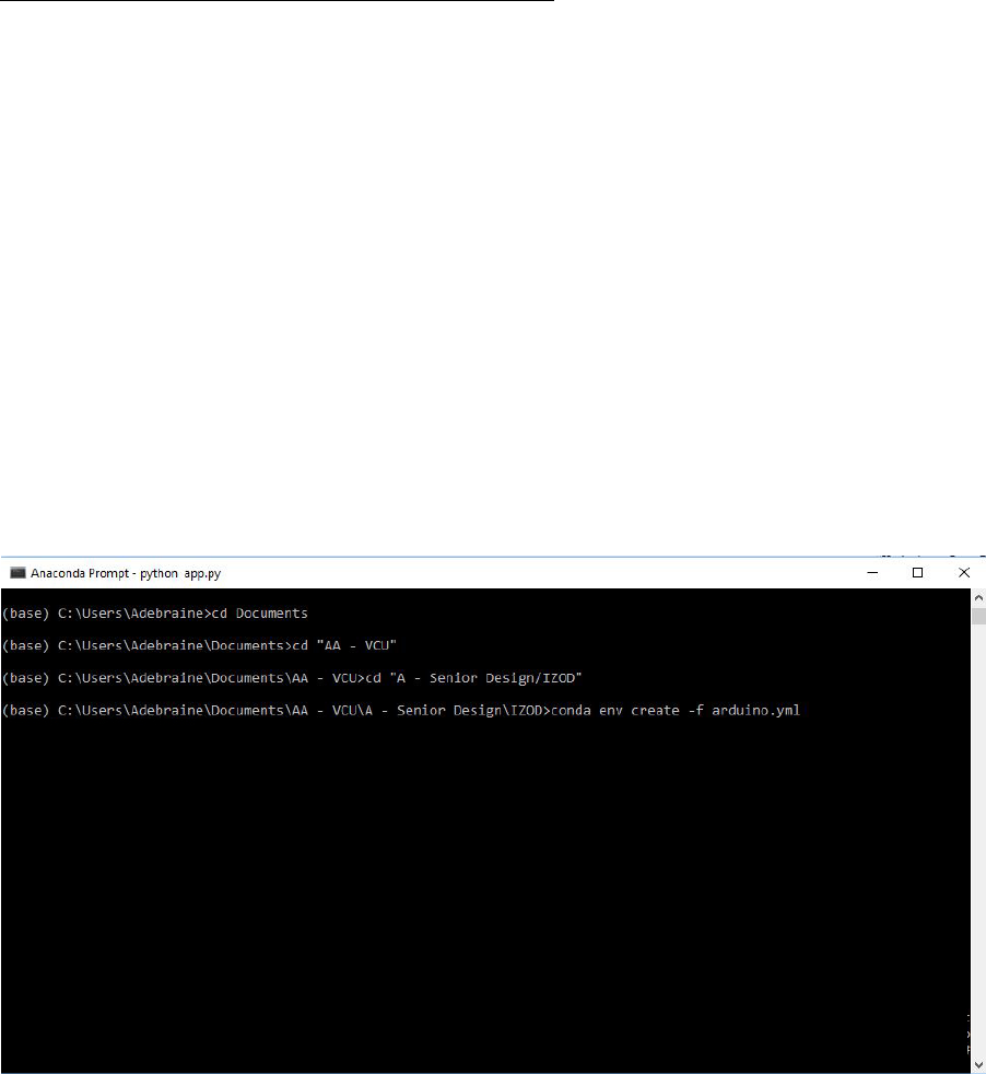
Fig. 1.1
1. Extract IZOD.zip where you wish to run the software
2. open Anaconda Prompt
3. Navigate to the adequate directory using cd:
Type: cd "PASTE PATH HERE"
Example: cd "C:\Users\Adebraine\Documents\AA - VCU\A - Senior Design\IZOD"
4. type conda env create -f arduino.yml
5. Ready to start the software
Figure 1.1: Install Arduino Environment
May 7, 2018 5 of 66
1.2. START SOFTWARE
1.2 START SOFTWARE
1.2.1 On Windows Using Anaconda Prompt
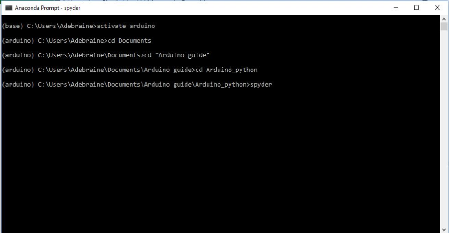
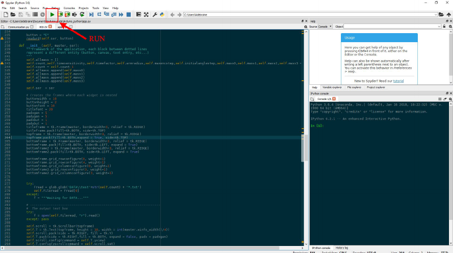
OPTION 1: Using Spyder (Fig. 1.2 & 1.3)
1. Connect the Arduino USB to the computer
2. Start Anaconda Prompt
3. Activate the arduino environment:
Type activate arduino
4. Navigate to the adequate directory using cd:
Type: cd "PASTE PATH HERE"
Example: cd "C:\Users\Adebraine\Documents\AA - VCU\A - Senior Design\IZOD"
5. Launch Spyder
6. Open app.py
7. press F5 or Click Run
Figure 1.2: Start Spyder Using Anaconda Prompt
May 7, 2018 6 of 66
1.2. START SOFTWARE
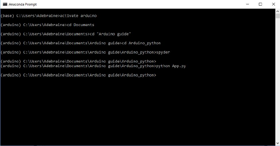
OPTION 2: Direct Launch through Anaconda Prompt(Fig. 1.4)
1. Connect the Arduino USB to the computer
2. Start Anaconda Prompt
3. Activate the arduino environment:
Type activate arduino
4. Navigate to the adequate directory using cd:
Type: cd "PASTE PATH HERE"
Example: cd "C:\Users\Adebraine\Documents\AA - VCU\A - Senior Design\IZOD"
5. Launch the Software:
Type python app.py
Figure 1.4: Start Software from Anaconda Prompt
May 7, 2018 8 of 66
1.3. FIND ZERO POSITION
1.3 FIND ZERO POSITION
1. Press CALIBRATION
2.
The arm will move a few degrees, disengage the magnet and wait until next command
is given
3. Wait until the hammer stops moving
4. Press CALIBRATION again
5.
the software will record the current position of the hammer before moving and set it as
ZERO
6.
The arm will come down and move the hammer to the position recorded in the prior
step
May 7, 2018 11 of 66
1.5. PERFORM A TEST
1.5 PERFORM A TEST
NOTE: Can be done from the LOADING position or from the ZERO position
1. Press RUN
2.
the arm will lift the hammer to the required 610mm +/- 2mm vertical height and
disengage the magnet
3. The hammer will come down and the software will record DATA for the first swing.
4. DATA is then automatically transformed, displayed on the GUI and saved in a text file
May 7, 2018 13 of 66
1.7. SOFTWARE INTERFACE DETAILS
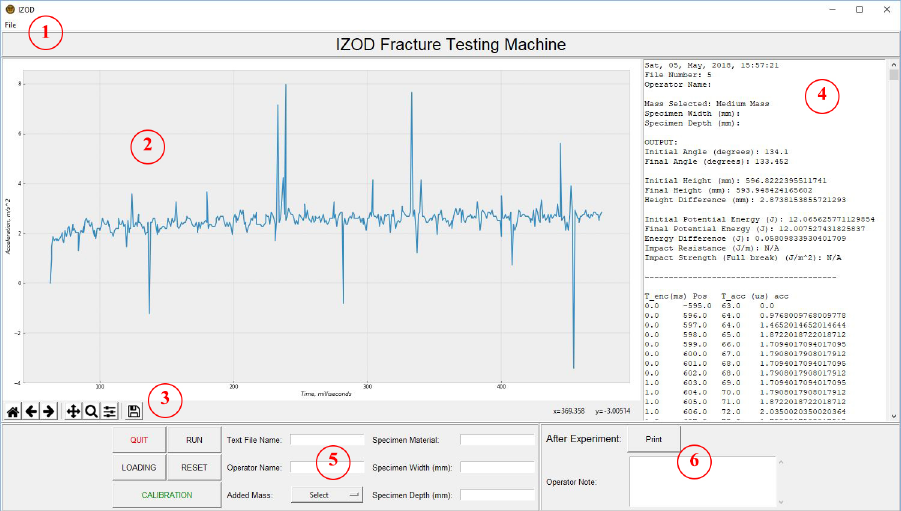
1.7 SOFTWARE INTERFACE DETAILS
1.7.1 Windows Desktop Version
1. FILE
Let’s the user access the
CHANGE DIRECTORY
function to decide where the next
Output text files will be saved
2. The Accelerometer output graph
3. Functions to manipulate and save the above graph
4. The Previous Test results (Identical to the output text file)
5. User input functions to enter BEFORE a test is performed, see below
6. User input function to enter AFTER a test is performed, see below
Figure 1.7: Windows GUI
May 7, 2018 15 of 66
1.7. SOFTWARE INTERFACE DETAILS
User Inputs BEFORE a Test is Performed:
NOTE: Make sure to properly press ENTER after writing anything in the different text boxes.
•Test File Name: Let’s the user edit the default output text file name.
Default format: IZOD{File count}_Date_{MM_DD_YYYY}_Time_{HH_MM_SS}
Example: IZOD6_Date_05_06_2018_Time_11_17_41
Edited format:
{User Input}_IZOD{File count}_Date_{MM_DD_YYYY}_Time_{HH_MM_SS}
Example: USERINPUT_IZOD6_Date_05_06_2018_Time_11_17_41
•Operator Name: Let’s the user add the name of the operator to the output text file
Appears in the text file as: Operator Name: User Input
Example: Operator Name: Dr. Guven
•Added Mass
: Choose between 4 default options: No added mass, small plates, medium
plates, and large plates
•Specimen Material: Let’s the user add the specimen material to the output text file
Appears in the text file as: Specimen Material: User Input
Example: Specimen Material: ABS
•Specimen Width (mm): Let’s the user specify the width of the specimen
Appears in the text file as: Specimen Width (mm): User Input
Example: Specimen Width (mm): 12.3
•Specimen Depth (mm): Let’s the user specify the Depth of the specimen at the notch
Appears in the text file as: Specimen Depth (mm): User Input
Example: Specimen Depth (mm): 12.3
May 7, 2018 16 of 66

1.7. SOFTWARE INTERFACE DETAILS
User Inputs AFTER a test is performed:
NOTE: Pressing ENTER does NOT save the note but allows the user to add a multi-line note.
1. Operator Note: Let’s the user add a note to the previous test’s output text file
Appears in the text file as: Operator Note: User Input
Example: Operator Note: Full break
2. Press PRINT to print the above note to the text file
May 7, 2018 17 of 66
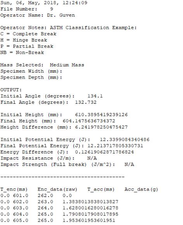
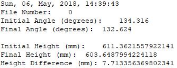
1.8. TEXT FILE OUTPUT DETAILS
1.8 TEXT FILE OUTPUT DETAILS
The text file will display N/A if the user did not enter required inputs.
The data is also saved below a dashed line in four columns:
• Time corresponding to the encoder data point in milliseconds
• Position of the hammer from 0 to 10,000 corresponding to 0 to 360 degrees.
• Time corresponding to the accelerometer data point in milliseconds
• accelerometer data point in g
Figure 1.9: Output Text File
May 7, 2018 19 of 66
2.2. SWAP WEIGHTS
2.2 SWAP WEIGHTS
IMPORTANT:
Each plate has its corresponding set of screws. Selecting the wrong set of
screws can lead to weights falling off, especially the large plates.
The user can switch the weights attached to the machine or remove all weights and select the
corresponding option on the GUI.
May 7, 2018 21 of 66
2.3. INVERT TOUCHSCREEN DISPLAY
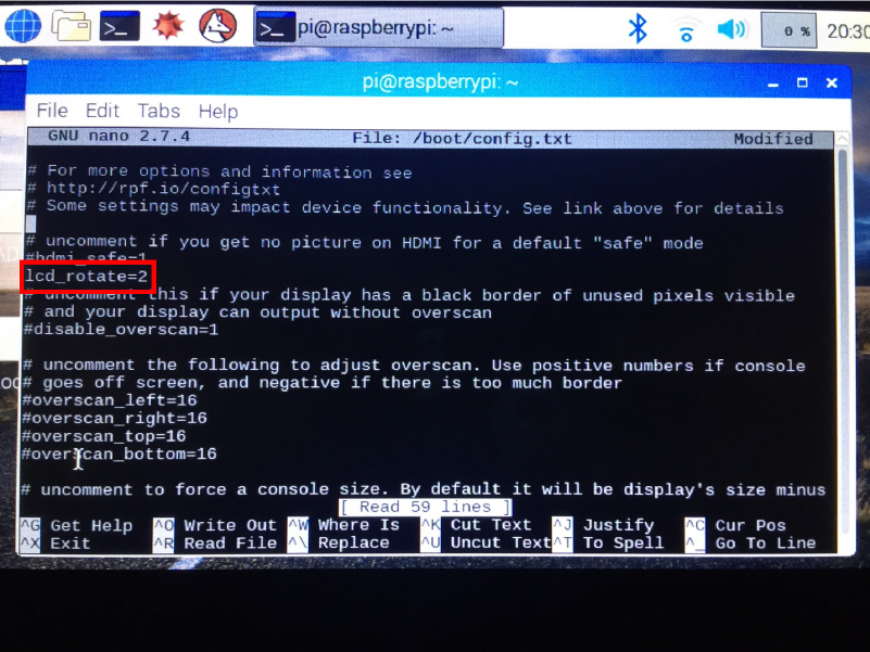
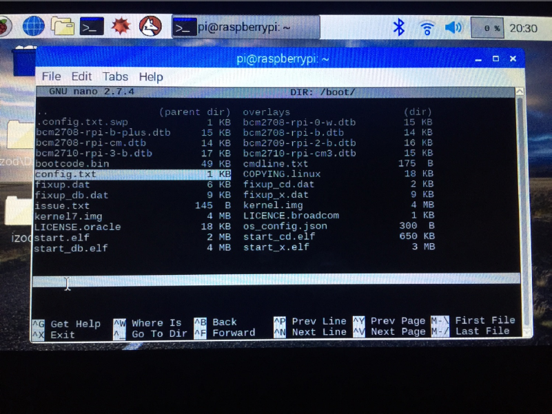
2.3 INVERT TOUCHSCREEN DISPLAY
Fig. 2.1 & 2.2
1. Open Terminal
2. Type sudo nano /boot/config.txt
3.
Type
lcd_rotate=0
or
lcd_rotate=2
depending on what is already there (DO NOT PRESS
ENTER)
4. Press CTRL + X
5. Press Y
6. Press CTRL + T
7. Press ARROW DOWN until you reach config.txt then press ENTER
8. type sudo reboot
Figure 2.1: Invert Touchscreen Display 1
May 7, 2018 22 of 66
2.4. INCORRECT ARM STARTING POSITION
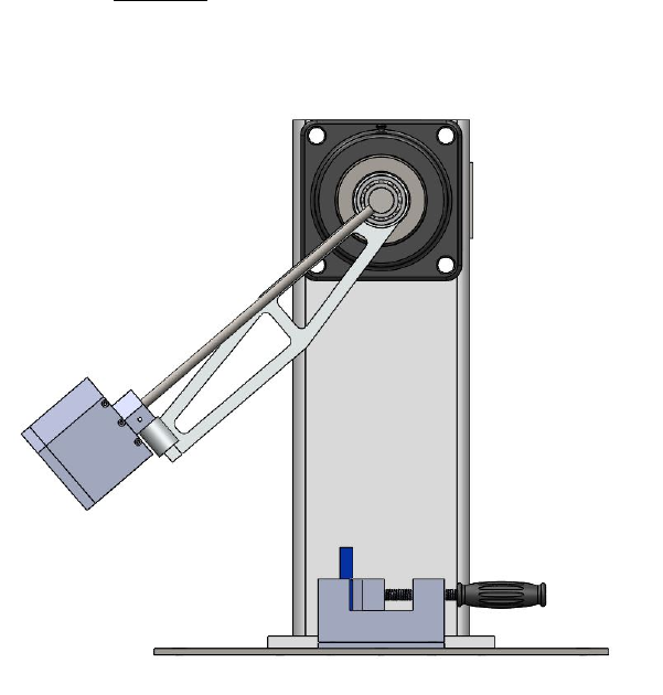
2.4 INCORRECT ARM STARTING POSITION
2.4.1 Arm Before ZERO Position
If the arm is located
between
the
ZERO
position and the
INITIAL MAXIMUM HEIGHT
position upon starting the software. Fig. 2.3
Figure 2.3: Arm before ZERO position
1. Press CALIBRATION on the GUI
2. Wait for the hammer to stabilize at the ZERO position (Full stop)
3. Press CALIBRATION again
4. Immediately move the hammer to the magnet on the arm.
May 7, 2018 24 of 66
2.4. INCORRECT ARM STARTING POSITION
2.4.2 Arm After ZERO Position
If the arm is located
between
the
ZERO
position and the
FINAL MAXIMUM HEIGHT
position upon starting the software. Fig. 2.4
Figure 2.4: Arm after ZERO position
1. Press CALIBRATION on the GUI
2. Wait for the arm to stop
3. Press CALIBRATION
4. Wait for the arm to stop
5. Repeat until the hammer reaches a position close to the ZERO position
6. Follow the calibration procedure, Section 1.3
May 7, 2018 25 of 66
2.5. UNRESPONSIVE SOFTWARE BUTTONS/ARDUINO COMMUNICATION
MALFUNCTION
2.5 UNRESPONSIVE SOFTWARE BUTTONS/ARDUINO COMMU-
NICATION MALFUNCTION
Typically, when the software is unresponsive or if it isn’t able to communicate with the
arduino it will return an error like the following:
could not open port ’com8’: FileNotFoundError(2, ’The system cannot find the file speci-
fied.’, None, 2)
It can be solved by first shutting down the software and unplugging/replugging the USB
connected to the Arduino from either the Raspberry Pi or the Computer used for operation.
May 7, 2018 26 of 66
2.6. BYPASS SOFTWARE INTERFACE
2.6 BYPASS SOFTWARE INTERFACE
The machine can be operated while bypassing the software, however the output text file
is minimal. See Fig. 2.5 for an example of the Output text file for this method.
1. Open Terminal on Raspbian or Anaconda Prompt on Windows
2. Type python Communication.py
3. Type B,C,D,E,Qadequately following:
(a) B:RUN
(b) C:RESET
(c) D:LOADING
(d) E:CALIBRATION
(e) Q:QUIT
Figure 2.5: Software Bypass Output Text File
May 7, 2018 27 of 66

CONTINUED ON BACK →
Why do I need
Anaconda Distribution?
What is
Anaconda Distribution?
Then what is Miniconda?
Will it work on
my machine?
Quick install it
Get your conda cheat sheet
Take the test drive
Installing Python in a terminal is no joy. Many scientific packages require a specific version
of Python to run, and it's dicult to keep them from interacting with each other. It is even
harder to keep them updated. Anaconda Distribution makes getting and maintaining
these packages quick and easy.
It is an open source, easy-to-install high performance Python and R distribution, with the
conda package and environment manager and collection of 1,000+ open source packages
with free community support.
It’s Anaconda Distribution without the collection of 1,000+ open source packages.
With Miniconda you install only the packages you want with the conda command,
conda install PACKAGENAME
Example: conda install anaconda-navigator
BEFORE YOU START
GET IT
Included in Anaconda 4.4+, or get with "conda install PACKAGENAME"
1. NumPy
numpy.org
N-dimensional array for numerical computation
2. SciPy
scipy.org
Scientific computing library for Python
3. Matplotlib
matplotlib.org
2D Plotting library for Python
4. Pandas
pandas.pydata.org
Powerful Python data structures
and data analysis toolkit
5. Seaborn
seaborn.pydata.org/
Statistical graphics library for Python
6. Bokeh
bokeh.pydata.org
Interactive web visualization library
7. Scikit-Learn
scikit-learn.org/stable
Python modules for machine learning and data mining
8. NLTK
nltk.org
Natural language toolkit
9. Jupyter Notebook
jupyter.org
Web app that allows you to create and share
documents that contain live code, equations,
visualizations and explanatory text
10. R essentials
conda.pydata.org/docs/r-with-conda.html
R with 80+ of the most used R packages for data science
“conda install r-essentials”
R package list
docs.anaconda.com/anaconda/rlanguage-pkg-docs
NOW PLAY WITH THE WORLD'S MOST AWESOME SCIENTIFIC PACKAGES
Yes, Anaconda Distribution is available for Windows, macOS or Linux x86 or POWER8,
32- or 64-bit, 3GB HD available. Miniconda is the same but needs only 400 MB HD.
docs.anaconda.com/anaconda/install
conda.io/docs/using/cheatsheet.html
conda.io/docs/test-drive.html
ANACONDA DISTRIBUTION
STARTER GUIDE
See full documentation for Anaconda Distribution
docs.anaconda.com/anaconda/
2.9. ANACONDA STARTER GUIDE
2.9 ANACONDA STARTER GUIDE
May 7, 2018 30 of 66

anaconda.com · info@anaconda.com · 512-776-1066
8/20/2017
Follow us on Twitter @anacondainc and join the #AnacondaCrew!
Connect with talented, like-minded data scientists and developers while contributing to the open source movement. Visit
anaconda.com/community.
ANACONDA NAVIGATOR
CHEAT SHEET
See full documentation for Anaconda Navigator
docs.anaconda.com/anaconda/navigator/
What is
Anaconda Navigator?
Anaconda Navigator is an easy way to use graphical Python programs without having to
use command line commands.
Before you Start
Get It
Free email group support
Paid support
Training
Consulting
http://bit.ly/anaconda-community
anaconda.com/anaconda-support
anaconda.com/training
anaconda.com/anaconda-consulting
MORE RESOURCES
Will it work on
my machine?
Follow the graphical
install instructions
Open
Anaconda Navigator
Anaconda Navigator is available for Windows, macOS or Linux, 32- or 64-bit, 3GB HD
available. Navigator is automatically installed when you install Anaconda Distribution.
docs.anaconda.com/anaconda/install
After install, look on your desktop or programs menu for Anaconda Navigator and click it.
NOW PLAY WITH THE WORLD'S MOST AWESOME SCIENTIFIC PACKAGES
2.9. ANACONDA STARTER GUIDE
May 7, 2018 31 of 66

CONDA CHEAT SHEET
Command line package and environment manager
Learn to use conda in 30 minutes at bit.ly/tryconda TIP: Anaconda Navigator is a graphical interface to use conda.
Double-click the Navigator icon on your desktop or in a Terminal or at
the Anaconda prompt, type anaconda-navigator
CONTINUED ON BACK →
conda info
conda update conda
conda install PACKAGENAME
spyder
conda update PACKAGENAME
COMMANDNAME --help
conda install --help
Conda basics
Verify conda is installed, check version number
Update conda to the current version
Install a package included in Anaconda
Run a package after install, example Spyder*
Update any installed program
Command line help
*Must be installed and have a deployable command,
usually PACKAGENAME
conda create --name py35 python=3.5
WINDOWS: activate py35
LINUX, macOS: source activate py35
conda env list
conda create --clone py35 --name py35-2
conda list
conda list --revisions
conda install --revision 2
conda list --explicit > bio-env.txt
conda env remove --name bio-env
WINDOWS: deactivate
macOS, LINUX: source deactivate
conda env create --le bio-env.txt
conda create --name bio-env biopython
Use conda to search for a package
See list of all packages in Anaconda
conda search PACKAGENAME
https://docs.anaconda.com/anaconda/packages/pkg-docs
Finding conda packages
Using environments
Create a new environment named py35, install Python 3.5
Activate the new environment to use it
Get a list of all my environments, active
environment is shown with *
Make exact copy of an environment
List all packages and versions installed in active environment
List the history of each change to the current environment
Restore environment to a previous revision
Save environment to a text file
Delete an environment and everything in it
Deactivate the current environment
Create environment from a text file
Stack commands: create a new environment, name
it bio-env and install the biopython package
2.10. CONDA CHEAT SHEET
2.10 CONDA CHEAT SHEET
May 7, 2018 32 of 66

conda create --name py34 python=3.4
Windows: activate py34
Linux, macOS: source activate py34
Windows: where python
Linux, macOS: which -a python
python --version
Installing and updating packages
Install a new package (Jupyter Notebook)
in the active environment
Run an installed package (Jupyter Notebook)
Install a new package (toolz) in a dierent environment
(bio-env)
Update a package in the current environment
Install a package (boltons) from a specific channel
(conda-forge)
Install a package directly from PyPI into the current active
environment using pip
Remove one or more packages (toolz, boltons)
from a specific environment (bio-env)
Specifying version numbers
Ways to specify a package version number for use with conda create or conda install commands, and in meta.yaml files.
Constraint type Specification Result
Fuzzy numpy=1.11 1.11.0, 1.11.1, 1.11.2, 1.11.18 etc.
Exact numpy==1.11 1.11.0
Greater than or equal to "numpy>=1.11" 1.11.0 or higher
OR "numpy=1.11.1|1.11.3" 1.11.1, 1.11.3
AND "numpy>=1.8,<2" 1.8, 1.9, not 2.0
NOTE: Quotation marks must be used when your specification contains a space or any of these characters: > < | *
Free Community Support
Online Documentation
Command Reference
Paid Support Options
Anaconda Onsite Training Courses
Anaconda Consulting Services
groups.google.com/a/continuum.io/forum/#!forum/conda
conda.io/docs
conda.io/docs/commands
anaconda.com/support
anaconda.com/training
anaconda.com/consulting
MORE RESOURCES
Follow us on Twitter @anacondainc and join the #AnacondaCrew!
Connect with other talented, like-minded data scientists and developers while
contributing to the open source movement. Visit anaconda.com/community
anaconda.com · info@anaconda.com · 512-776-1066
8/20/2017 conda cheat sheet Version 4.3.24
Managing multiple versions of Python
Install dierent version of Python in
a new environment named py34
Switch to the new environment that has
a dierent version of Python
Show the locations of all versions of Python that are
currently in the path
NOTE: The first version of Python in the list will be executed.
Show version information for the current active Python
conda install jupyter
jupyter-notebook
conda install --name bio-env toolz
conda update scikit-learn
conda install --channel conda-forge
boltons
pip install boltons
conda remove --name bio-env toolz boltons
2.10. CONDA CHEAT SHEET
May 7, 2018 33 of 66
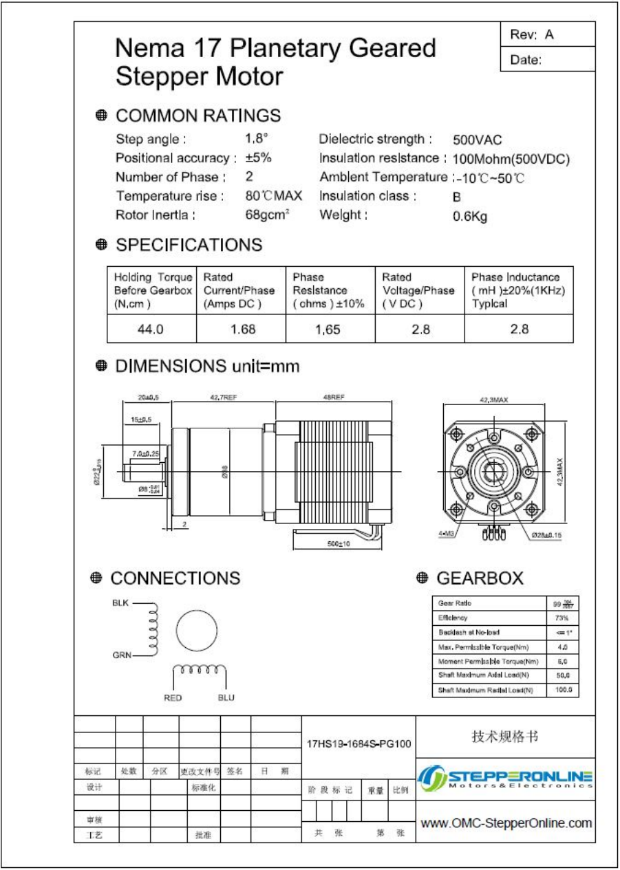
3.5. NEMA17 100:1 STEPPER MOTOR
3.5 NEMA17 100:1 STEPPER MOTOR
Electrical Specification:
* Manufacturer Part Number: 17HS19-1684S-PG100
* Motor Type: Bipolar Stepper
* Step Angle: 0.018 deg.
* Holding Torque: 4Nm
* Rated Current/phase: 1.68A
* Phase Resistance: 1.65ohms
* Inductance: 2.8mH+/-20%(1KHz)
Gearbox Specifications:
* Gearbox Type: Planetary
* Gear Ratio: 99.05:1
* Efficiency: 73%
* Backlash at No-load: <=1 deg.
* Max.Permissible Torque: 4Nm(566oz-in)
* Moment Permissible Torque: 6Nm(850oz-in)
* Shaft Maximum Axial Load: 50N
* Shaft Maximum Radial Load: 100N
Physical Specifications:
* Frame Size: 42 x 42mm
* Motor Length: 48mm
* Gearbox Length: 42.7mm
* Shaft Diameter: 8mm
* Shaft Length: 20mm
* D-cut Length: 15mm
* Number of Leads: 4
* Lead Length: 500mm
* Weight: 630g
Connection:
Black(A+), Green(A-), Red(B+), Blue(B-)
May 7, 2018 47 of 66
1 of 2
Wachendorff Automation GmbH & Co. KG
Industriestraße 7 • D-65366 Geisenheim
Tel.: +49 (0) 67 22 / 99 65-25 • Fax: +49 (0) 67 22/ 99 65 -70
E-Mail: wdg@wachendorff.de • www.wachendorff-automation.com
27.04.2010 / Specifications without engagement, subject to errors and modifications.
Cable connection K2, K3, L2, L3 with 2 m cable
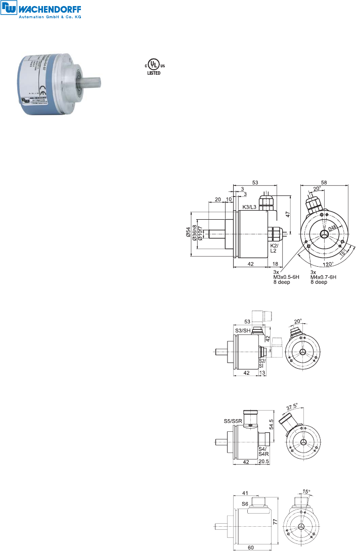
Connector (M16x0.75) SI, SH, 5-, 6-, 8-, 12-pin and S2, S3, 7-pin
Encoder WDG 58B
Available PPR up to 25000 PPR
Mechanical Data
Housing
- Clamping flange: Aluminium
- Cap: Aluminium, powder coated
- Cam mounting: pitch 69 mm
Shaft Ø 10 mm
- Material: stainless steel
- Permitted load max. 220 N radial
on shaft end: max. 120 N axial
- Starting torque: approx. 1 Ncm at ambient temperature
Bearings
- Type: 2 precision ball bearings
- Service life: 1 x 10⁹revs. at 100 % rated shaft load
1 x 10¹⁰ revs. at 40 % rated shaft load
1 x 10¹¹ revs. at 20 % rated shaft load
Max. operating speed: 8000 rpm
Weight: approx. 250 g
Connections: cable or connector
Protection rating: IP67, shaft sealed to IP65
(EN 60529)
Operating temperature: -20 °C up to +80 °C, 1 Vss: -10 °C up to +70 °C
Storage temperature: -30 °C up to +80 °C
Machinery Directive: basic data safety integrity level
MTTFd: 200 a
Mission time (TM): 25 a
Nominale service life 1 x 10¹¹ revss. at 8000 rpm and 20 % rated
(L10h): shaft load
Diagnostic coverage (DC): 0 %
Electrical Data
Power supply/ 4.75 VDC up to 5.5 VDC: max. 100 mA
Open circuit current 5 VDC up to 30 VDC: max. 70 mA
consuption: 10 VDC up to 30 VDC: max. 100 mA
Output circuit: TTL, RS422 compatible
HTL
1 Vss Sin/Cos
Pulse frequency: TTL ≤ 5000 PPR: max. 200 kHz
HTL ≤ 5000 PPR: max. 200 kHz
TTL > 5000 PPR: max. 2 MHz
HTL > 5000 PPR: max. 600 kHz
1 Vss Sin/Cos: max. 100 kHz
Channels: AB, ABN and inverted signals
Load: max. 40 mA / channel,
@ 1 Vss Sin/Cos: 120 Ohm termination
Circuit protection: circuit type F24, G24, H24, I24, P24, R24 only
Accuracy: Phase offset: 90° ± max. 7.5 %
of the pulse length
pulse-/pause-ratio: 50 % ± max. 7 %
Connector (M23) S4, S5, S4R, S5R, 12-pin
• Rugged industrial standard encoder
• Up to 25000 PPR by use of high grad electronics
• Protection to IP67, shaft sealed to IP65
• Maximum mechanical and electrical safety
• Full connection protection with 10 VDC up to 30 VDC
• With light reserve warning
• Optional: -40 °C up to +80 °C
Protection to IP67 all around
www.wachendorff-automation.com/wdg58b
MIL-connector S6, 6-pin
Further technical information on:
www.wachendorff-automation.com/gtd
Matching accessories on: www.wachendorff-automation.com/acs
3.6. ENCODER
3.6 ENCODER
May 7, 2018 49 of 66
2 of 2
Pulses per revolution PPR:
2, 10, 15, 20, 24, 25, 30, 36, 40, 48, 50, 60, 64, 72, 87, 90, 100, 120,
125, 127, 128, 150, 160, 180, 200, 216, 240, 250, 254, 256, 300,
314, 320, 360, 400, 500, 512, 571, 600, 625, 720, 750, 768, 800,
810, 900, 1000, 1024, 1200, 1250, 1270, 1440, 1500, 1800, 2000,
2048, 2400, 2500, 3000, 3600, 4000, 4096, 4685, 5000, 10000,
12500, 20000, 25000.
1 Vss Sin/Cos 1024 PPR and 2048 PPR only
Other PPRs on request
Ordering information:
Options:
Empty = Without option
ACA = Low-temperature -40 °C up to +80 °C
AAF = Shaft with flat
AAC = Low-friction bearings
AAO = Shaft sealed to IP67
In decimetres = Cable length
WDG 58B
WDG 58B
5000 ABN G24 K2
Example
Your encoder
Valve-connector S7, 4-pin Shaft with flat:
The encoder WDG 58B can be supplied with a shaft with flat. When
ordering please add the suffix code - AAF.
Low-friction bearings:
The encoder WDG 58B is also available as a particularly smooth-running
low-friction encoder. The starting torque is thereby changed to
<0.1 Ncm and the protection class at the shaft input to IP50. When
ordering please add the suffix code - AAC.
Amended specifications for shaft sealed to IP67.
Shafts sealed to IP67 (not for 1 Vss Sin/Cos):
The encoder WDG 58B can be supplied in a full IP67 version. When
ordering please add the suffix code - AAO.
Max.
RPM
Permitted
Shaft-Loading
axial radial
Max.
PPR
Starting-
torque
3500 rpm 100 N 110 N 2500 PPR approx. 4 Ncm
Drawing 58B-AAF
Cable length:
The encoder WDG 58B can be supplied with more than 2 m cable.
The maximum cable length depends on the supply voltage and the
frequency; see "General Technical Data":
www.wachendorff-automation.com/gtd
Please extend the standard order code with a three figure number,
specifying the cable length in decimetres.
Example: 3 m cable = 030
Order No.:
Electrical connections: ABN
inv.
Order key Outgoing Description
Cable: (Length 2 m standard)
K2 axial shield not connected •
L2 shield connected to encoder housing •
K3 radial shield not connected •
L3 shield connected to encoder housing •
Connector:
SI5 axial 5-pin, connector -
SH5 radial
SI6 axial 6-pin, connector -
SH6 radial
SI8 axial 8-pin, connector •
SH8 radial
SI12 axial 12-pin, connector •
SH12 radial
S2 axial 7-pin, connector -
S3 radial
S4/S4R axial 12-pin, connector
(R = clockwise pin count) •
S5/S5R radial
S6 axial 6-pin, MIL-connector -
S7 radial 4-pin, Valve-connector -
SB4 axial 4-pin, M12-sensor-connector -
SC4 radial
SB5 axial 5-pin, M12-sensor-connector -
SC5 radial
SB8 axial 8-pin, M12-sensor-connector •
SC8 radial
SB12 axial 12-pin, M12-sensor-connector •
SC12 radial
Channels: AB, ABN (SIN: AB)
Sensor-connector (M12x1) SB, SC, 4-, 5-, 8-, 12-pin
All dimensional specifications in mm.
Options:
Low-temperature:
The encoder WDG 58B with the output circuit types F24, G24, H24, I24,
P24, R24, F05, G05, I05, P05, 245 and 645 is also available with the
extended temperature range -40 °C up to +80 °C (measured at the flan-
ge). When ordering please add the suffix code - ACA.
Please see our general technical data at: www.wachendorff-automation.com/gtd
Output circuit:
Reso-
lution
PPR
Power
supply
VDC
Output circuit Light
reserve
warning
Order
Key
up to
1024
5 - 30 HTL -H30
HTL inverted -R30
up to
5000
4,75 - 5,5 TTL •G05
-H05
TTL,
RS422 comp., inverted
•I05
-R05
10 - 30 HTL •G24
-H24
HTL inverted •I24
-R24
TTL, RS422 comp., inv. •245
10000
up to
25000
4,75 - 5,5 TTL -F05
TTL, RS422 comp., inv. -P05
10 - 30 HTL -F24
HTL inverted -P24
TTL, RS422 comp., inv. -645
up to
2048
4,75 - 5,5 1 Vss Sin/Cos -SIN
3.6. ENCODER
May 7, 2018 50 of 66
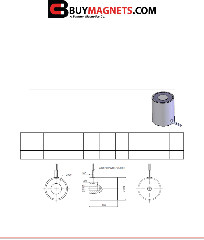
1150 Howard Street • Elk Grove Village, IL 60007 • 800-232-4359 or 847-593-2060
Technical Data Sheet
Round Electromagnets, Flat-Faced
BuyMagnets.com Round electromagnets handle ferrous materials safely and
securely. Electromagnets provide an efficient and economical solution for handling
and holding parts. Available in a number of shapes and sizes, our electromagnets
require little maintenance and can be used in a variety of manual and automated
applications. (Special sizes upon request).
Product Specifications
Shape: Round
Part No.
Diameter(A)
Height
(B)
Thread
(C)
Thread
Depth
(D)
DC
Volts
Watts
Pull
Force
Wt.
Price
BDE-1012-
12
1.00
1.250
10-32
.375
12
4.5
20
2.60oz
$20.00
All Measurements are in inches (unless otherwise noted)
Direction of Magnetization (DOM) is through the thickness unless noted
Unless otherwise specified, magnets will be furnished in magnetized condition
Holding forces are approximate. These are average values obtained under laboratory conditions.
Size, shape, and material of the test piece may affect actual pull forces
3.7. ELECTRO-MAGNET
3.7 ELECTRO-MAGNET
May 7, 2018 51 of 66
Chapter 4
ASTM Methodologies
NOTE: Information directly extracted from ASTM D256
Refer to ASTM D256 for more in-depth details.
4.1 MEASURING EFFECTIVE WEIGHT OF THE HAMMER
Swing the pendulum to a horizontal position and support it by the striking edge in this
position with a vertical bar. Allow the other end of this bar to rest at the center of a load
pan on a balanced scale. Subtract the weight of the bar from the total weight to find the
effective weight of the pendulum. The effective pendulum weight should be within 0.4%
of the required weight for that pendulum capacity. If weight must be added or removed,
take care to balance the added or removed weight without affecting the center of percussion
relative to the striking edge. It is not advisable to add weight to the opposite side of the
bearing axis from the striking edge to decrease the effective weight of the pendulum since the
distributed mass can lead to large energy losses from vibration of the pendulum.
May 7, 2018 63 of 66
4.2. MEASURING EFFECTIVE LENGTH OF THE HAMMER
4.2 MEASURING EFFECTIVE LENGTH OF THE HAMMER
The distance from the axis of support to the center of percussion may be determined experi-
mentally from the period of small amplitude oscillations of the pendulum by means of the
following equation:
L=(g/(4π2)p2
where:
L = distance from the axis of support to the center of percussion, mor (f t)
g = local gravitational acceleration (known to an accuracy of one part in one thousand),
m
/
s2
or (f t/s2), π=3.1416 (4π2=39.48)
p = period,
s
, of a single complete swing (to and fro) determined by averaging at least 20
consecutive and uninterrupted swings. The angle of swing shall be less than 5 degrees each
side of center.
May 7, 2018 64 of 66
4.3. SPECIMEN FAILURE TYPES
4.3 SPECIMEN FAILURE TYPES
The type of failure for each specimen shall be recorded as one of the four categories listed as
follows:
1. C = Complete Break: A break where the specimen separates into two or more pieces.
2.
H = Hinge Break: An incomplete break, such that one part of the specimen cannot
support itself above the horizontal when the other part is held vertically (less than 90¡r
included angle).
3.
P = Partial Break: An incomplete break that does not meet the definition for a hinge
break but has fractured at least 90% of the distance between the vertex of the notch and
the opposite side.
4.
NB = Non-Break: An incomplete break where the fracture extends less than 90% of the
distance between the vertex of the notch and the opposite side.
May 7, 2018 65 of 66
4.4. SPECIMEN DIMENSIONS FOR IZOD-TYPE TEST
4.4 SPECIMEN DIMENSIONS FOR IZOD-TYPE TEST
1. A = 10.16 +/−0.05 mm or 0.400 +/−0.002 in
2. B = 31.8 +/−1.0 mm or 1.25 +/−0.04 in
3. C = 63.5 +/−2.0 mm or 2.50 +/−0.08 in
4. D = 0.25R +/−0.05 mm or 0.010R +/−0.002 in
5. E = 12.70 +/−0.20 mm or 0.500 +/−0.008 in
Figure 4.1: Specimen Dimensions
May 7, 2018 66 of 66
