Phoebe Manual
User Manual:
Open the PDF directly: View PDF ![]() .
.
Page Count: 21
VILLANOVA UNIVERSITY
DEPT. OF ASTRONOMY AND ASTROPHYSICS
PHOEBE manual
Andrej Prˇsa (Villanova University, PA, USA)
Petr Harmanec (Charles University, Prague, CZ)
Adopted for PHOEBE 0.32
13 April 2010
CONTENTS 2
Contents
1 Introduction 3
1.1 PHOEBE license .......................... 3
2 Heads-up! 5
3 Running PHOEBE for the first time 5
4 Starting a new project in PHOEBE 7
4.1 Inputdata............................. 9
4.2 Passbands............................. 10
4.3 Dataweighting .......................... 15
4.4 Propagating formal errors . . . . . . . . . . . . . . . . . . . . 17
5 SOLVING THE INVERSE TASK IN PHOEBE 20
5.1 DIFFERENTIAL CORRECTIONS . . . . . . . . . . . . . . . 20
5.2 NELDER AND MEAD SIMPLEX . . . . . . . . . . . . . . . 20
5.3 USING THE SCRIPTER . . . . . . . . . . . . . . . . . . . . 20
6 OUTPUT OF RESULTS 20
1 INTRODUCTION 3
1 Introduction
PHOEBE stands for PHysics OfEclipsing BinariEs. It is a tool for the modeling
of eclipsing binary stars based on photometric and spectroscopic (radial ve-
locity) data. PHOEBE is based on the Wilson and Devinney (1971, hereafter
WD) code.
PHOEBE is pronounced fee-bee.
The suite consists of three parts:
•The library: phoebe-lib
This is PHOEBE’s scientific and computational core. It contains functions
and algorithms that are used for eclipsing binary modeling. It is not
a stand-alone application. As such, it cannot be run, nor can it be
used in any direct fashion. For interaction with the user, a driver is
needed. Provided are two drivers: the GUI and the scripter. These are
the front-ends the user sees.
•The graphical user interface: phoebe-gui
PHOEBE’s graphical user interface (GUI) is a heavily structured front-
end for setting parameter values, plotting light and radial velocity
curves, invoking the minimizer and overviewing the model results. The
GUI is especially suited for the case-by-case analysis. This manual will
predominantly focus on the GUI.
•The scripter: phoebe-scripter
The scripter is a terminal-based front-end that features a full-fledged
scripting language developed especially for PHOEBE. It requires a some-
what steep learning curve, to the profit of flexibility and the power
of scripting. The scripter may prove useful to users with at least su-
perficial experience in working with the GUI and eclipsing binaries in
general. It is especially suited for statistical tests and analysis of larger
data-sets.
1.1 PHOEBE license
PHOEBE is and will always be free: both free of charge and free in a sense
that you may re-use its code in any way you see fit. PHOEBE is released under
the GNU General Public Licence. A copy of the licence can be found in the
top-level COPYING file of the distribution. To quote the most important part:
1.1 PHOEBE license 4
The licenses for most software are designed to take away your
freedom to share and change it. By contrast, the GNU General
Public License is intended to guarantee your freedom to share
and change free software–to make sure the software is free for all
its users. This General Public License applies to most of the Free
Software Foundation’s software and to any other program whose
authors commit to using it. (Some other Free Software Foun-
dation software is covered by the GNU Library General Public
License instead.) You can apply it to your programs, too.
When we speak of free software, we are referring to freedom,
not price. Our General Public Licenses are designed to make sure
that you have the freedom to distribute copies of free software
(and charge for this service if you wish), that you receive source
code or can get it if you want it, that you can change the software
or use pieces of it in new free programs; and that you know you
can do these things.
To protect your rights, we need to make restrictions that for-
bid anyone to deny you these rights or to ask you to surrender
the rights. These restrictions translate to certain responsibilities
for you if you distribute copies of the software, or if you modify
it.
For example, if you distribute copies of such a program, whe-
ther gratis or for a fee, you must give the recipients all the rights
that you have. You must make sure that they, too, receive or can
get the source code. And you must show them these terms so
they know their rights.
We protect your rights with two steps: (1) copyright the soft-
ware, and (2) offer you this license which gives you legal permis-
sion to copy, distribute and/or modify the software.
Also, for each author’s protection and ours, we want to make
certain that everyone understands that there is no warranty for
this free software. If the software is modified by someone else and
passed on, we want its recipients to know that what they have is
not the original, so that any problems introduced by others will
not reflect on the original authors’ reputations.
Finally, any free program is threatened constantly by software
patents. We wish to avoid the danger that redistributors of a free
program will individually obtain patent licenses, in effect making
the program proprietary. To prevent this, we have made it clear
that any patent must be licensed for everyone’s free use or not
licensed at all.
2 HEADS-UP! 5
2 Heads-up!
PHOEBE is based1on the approximation of stellar shapes by equipotentials.
Thus, the program does not use common parameters such as semi-amplitudes
of the radial-velocity curves or relative photometric radii. Instead, the stellar
shapes are characterized by the values of equipotentials, the mass ratio and
semi-major axis. Note that, for proximity-distorted stars, the use of equipo-
tentials implies that the mass ratio is affected not only by RVs but also by
photometric data.
3 Running PHOEBE for the first time
In this section we will assume that the installation of PHOEBE and its compo-
nents is done correctly. Upon invocation, PHOEBE looks for the configuration
file phoebe.config in the following locations:
•~/.phoebe-0.32, a hidden directory in your home directory. This cor-
responds to the current PHOEBE installation;
•~/.phoebe-0.xy, where xy are all official PHOEBE releases. This cor-
responds to all legacy PHOEBE installations, and configuration settings
will be imported.
If the configuration file is not found in any of the above locations, you
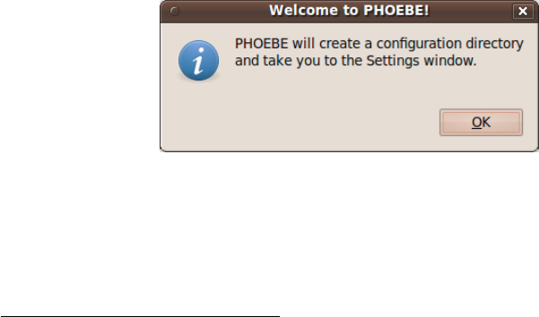
will be presented with the following notice window:
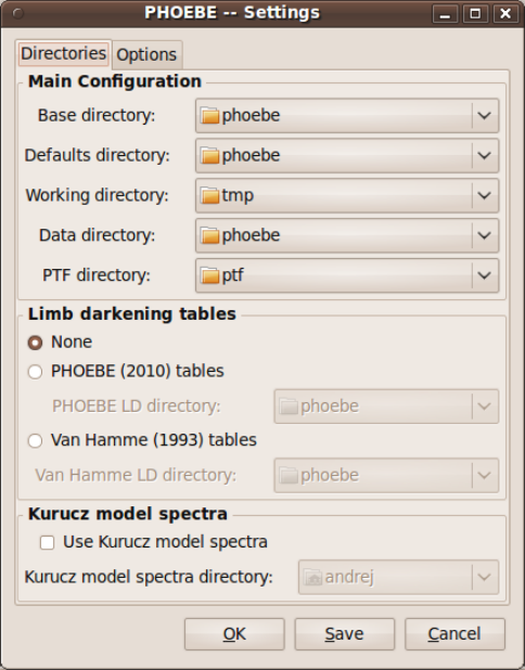
Upon clicking on OK, a Settings window will appear. The settings are
split into two tabs: Directories and Options. The Base directory is where
PHOEBE expects to find the source code; the Defaults directory is a location
of the defaults.phoebe file. The purpose of this file is to make permanent
1Please refer to the PHOEBE Scientific Reference for the details on the model formula-
tion.
3 RUNNING PHOEBE FOR THE FIRST TIME 6
changes to the default values of parameters that PHOEBE uses upon start.
The Working directory is scratch space where PHOEBE outputs temporary
files (useful for control and debugging). The Data directory is where PHOEBE
expects to find parameter files; this is usually set up as a parent directory with
per-star subdirectories, i.e. projects/EBs might be a Data directory that
contains subdirectories such as projects/EBs/UWLMi etc. Finally, the PTF
directory contains Passband Transmission Functions supported by PHOEBE.
We will discuss these at length in §4.2.
Next, you can opt to use precomputed limb darkening (LD) tables; two
tables are currently supported, the internal LD tables computed from Castelli
and Kurucz (2004)’s NEWODF models, or van Hamme (1993) tables. Fi-
nally, as a part of work in progress, you may select a directory with Kurucz’s
model spectra; these will be used for full-fledged comparison between ob-
served and Kurucz’s spectra. This functionality, however, is not yet made
available for PHOEBE 0.32 due to insufficient testing.
The defaults for the directories are listed in Table 1. Make sure you change
the Data directory to something more appropriate, i.e. a subdirectory with
write access in your home directory.
4 STARTING A NEW PROJECT IN PHOEBE 7
Directory: Default:
Base /usr/local/share/phoebe
Defaults /usr/local/share/phoebe/defaults
Working /tmp
Data /usr/local/share/phoebe
PTF /usr/local/share/phoebe/ptf
Table 1: Default PHOEBE directories in the Settings window.
Take some time to review the Options tab of the Settings window. Cur-
rently there are only two options available, but more will be added as they
are implemented.
Once you have set up the directories, either click Save to permanently
store the settings in a configuration file, or click OK to use the settings tem-
porarily (they will be lost upon PHOEBE exit).
4 Starting a new project in PHOEBE
This section will guide you through an examplary PHOEBE run that includes
setting up and visualizing the data, and initializing the model. Upon a suc-
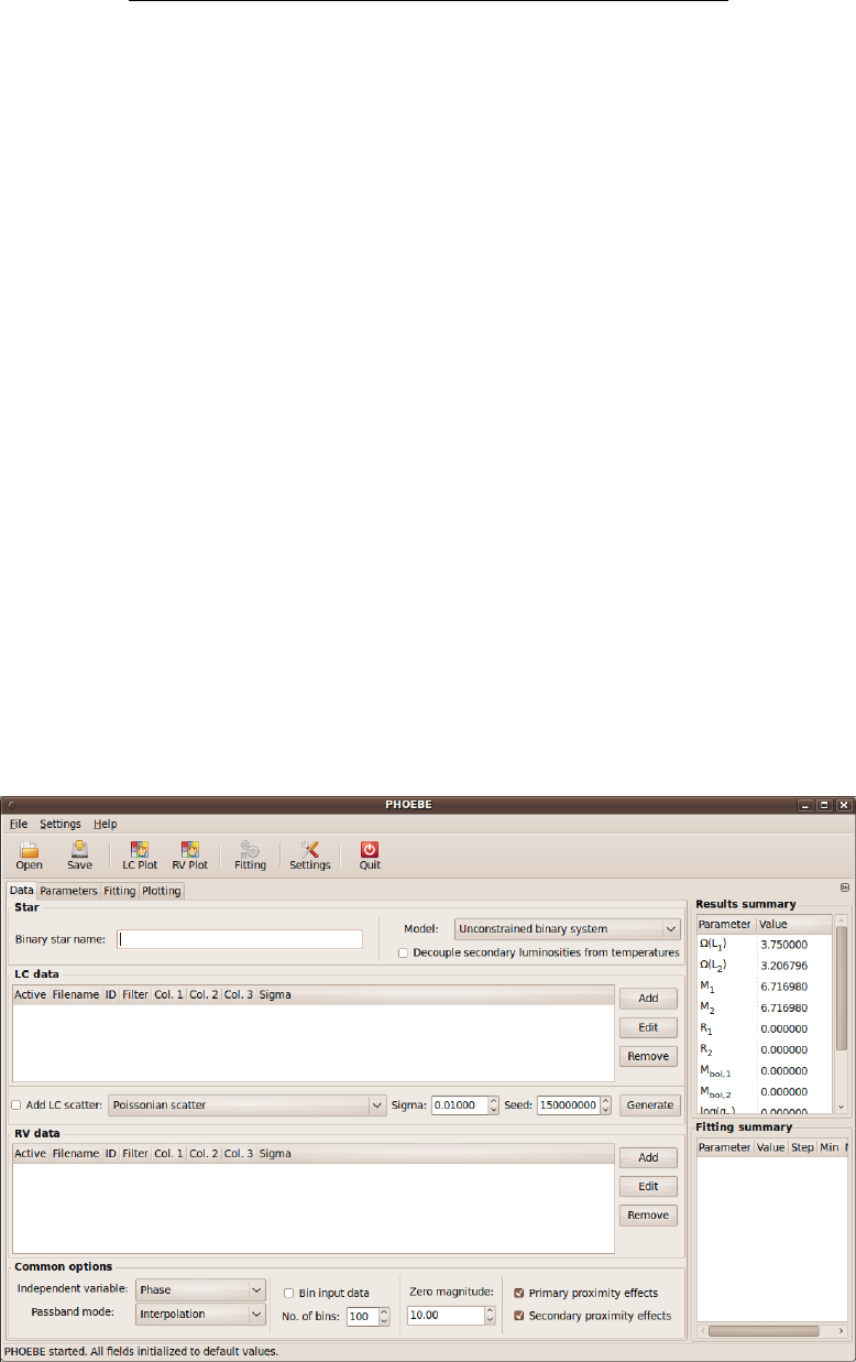
cessful initial configuration, you will be presented with the following screen.
4 STARTING A NEW PROJECT IN PHOEBE 8
We will be using a detached binary star UW LMi for all examples; the data
are distributed with PHOEBE, or you can download them from the following
location:
http://phoebe.fiz.uni-lj.si/files/UWLMi.tar.gz
Type in a name of your star in the Binary star name field; note that the
title of the PHOEBE window will change to include this name for reference.
If you have any prior information on the morphology of your star, select it
from the Model drop-down box. The options are:
X-Ray binary. This mode of operation relies on the accurate eclipse dura-
tion timing of the compact object available from X-Ray observations,
expressed in terms of the phase angle θ.
Unconstrained binary system. No morphology constraints are imposed.
Overcontact binary of W UMa type. In this mode the following con-
straints are applied: primary and secondary star potentials are equal;
polar temperature of the secondary star is computed by the gravity
darkening law of the entire common envelope; gravity darkening, bolo-
metric albedo and limb darkening parameters of both stars are the
same.
Detached binary. This mode is for detached binaries with no constraints
on the potentials.
Overcontact binary not in thermal contact. In this mode the compo-
nents are in geometric contact, but not in thermal contact. The pri-
mary and secondary potentials are thus constrained to be equal, but
the constraints on the gravity darkening, temperatures, albedoes and
limb darkening are not applied.
Semi-detached binary, primary fills the Roche lobe. This mode cor-
responds to the cases where the primary exactly fills its classical Roche
lobe; the only constraint is the value of the primary potential that is
set to its Roche lobe value.
Semi-detached binary, secondary fills the Roche lobe. Similar the the
previous mode, only that the secondary fills its Roche lobe, and accord-
ingly, the secondary star potential is constrained.
Double contact binary. In this mode both stars are filling their Roche
lobes exactly, and both values of the potential are constrained accord-
ingly.

4.1 Input data 9
# Object: UW LMi
# Passband: Johnson V
# Source: Crni Vrh Observatory, Slovenia
#
# HJD V StDev
2451642.366073 8.278 0.004
2451642.367797 8.288 0.004
2451642.369510 8.276 0.004
...........
Table 2: An example of the input data file.
In all but the unconstrained mode, the secondary star luminosity is
computed from the radiative properties rather than from the provided sec-
ondary luminosity parameters in the Parameters->Luminosities tab. This
constraint can be explicitly removed by checking the Decouple secondary
luminosities from temperatures option. Typically you do not want to
do this unless there is a good reason to not trust the radiative model.
If you are using UW LMi data, select Detached binary morphology and
make sure that secondary luminosities are not decoupled from temperatures.
4.1 Input data
PHOEBE can treat photometric and RV data either as a function of time (typ-
ically heliocentric Julian days) or orbital phase. In the current implementa-
tion it is possible to use many individual light curves in various photometric
passbands but only one set of RVs for the primary and another one for the
secondary. If the RV data come from various sources which do not have the
same RV zero point, the user has to correct these RV shifts in advance before
using such data in PHOEBE. Work is in progress to remove this limitation.
Observational data enter in a free format. Empty lines and white space
are handled gracefully. The comments are denoted with a #character; any-
thing that follows #and spans to the end of the line is ignored. The number
of comments is not limited. Observations typically contain 2 or 3 columns:
time (or phase), measured quantity (RV in km/s, magnitude or flux) and –
optionally – standard deviation or weight of the observation. Table 2 shows
an example of the photometric input data.
Note that no matter whether you specify magnitude or flux in the input

4.2 Passbands 10
Passband set: Passbands:
Johnson U,B,V,R,I,J,H,K,L,M,N
Cousins RC,IC
Geneva U,B,B1, B2, V,V1, G
Str¨omgren u,v,b,y,Hβ,n,Hβ,w
SDSS u,g,r,i,z
Bessell IR J,H,K,L,L0,M
HST complete FOC system
Hipparcos BT,VT,Hp
CoRoT exo, sismo
Kepler default
Table 3: Supported passbands in PHOEBE 0.32.
data file, the program internally always uses fluxes. For that reason you need
to specify the approximate magnitude of the binary at quarter-phase to have
to flux scale in a reasonable numeric range. This parameter is called Zero
magnitude appears in the Data tab.
4.2 Passbands
Every light curve has an associated passband with it, and every passband
is described by a transmission function (sometimes called response function)
that gives the transmission efficiency as function of wavelength. The trans-
mission function will typically be a combination of the filter response function
and the optics detection efficiency (i.e. reflective properties of the mirror,
CCD quantum efficiency, etc). However, when using standard photomet-
ric systems, such as Johnson, Cousins, Sloan, . . . , most instrumental effects
will be removed by data reduction. Then a passband transmission curve is
essentially the same as the filter response function.
The passband effects on the model are extensive and range from proper
account for the radiative physics to limb darkening corrections. The compu-
tation of these corrections is involved and computationally intensive, that is
why PHOEBE comes with precomputed lookup tables for these corrections, for
each passband. This implies that PHOEBE can handle only those passbands
for which the tables have been precomputed. Table 3 lists all passbands
supported by PHOEBE 0.32.
Since the observed features of radiative properties depend on the used
passband, a number of model parameters is passband-dependent: primary
and secondary passband luminosities, third light, interstellar extinction, limb
4.2 Passbands 11
darkening, etc. On top of that, the observations in each passband may be
weighted differently, according to the light level (cf. §4.3 for the details on
data weighting). This means that the proper passband selection is crucial
for the accurate synthetic light curve computation.
We are working on implementing custom passband support to PHOEBE;
in the mean time you can contact us on the phoebe-discuss mailing list
and request radiation and limb darkening tables to be computed for your
particular passband.
Radial velocity curves are no different, since the observed radiative fea-
tures depend on the observed wavelength interval. However, spectroscopic
data are rarely filtered and the passband transmission function depends pri-
marily on the properties of optics. Fortunately, the effects on the radial
velocity curves are limited to photometric corrections and are second order
effects, so the synthetic RV curves are not extremely sensitive to the passband
selection. What you typically want to do is select a passband that roughly
covers the wavelength range of the spectral lines used for RV determination.
§
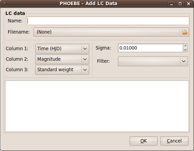
To add a new observational curve to PHOEBE, click on the Add button in
the LC data or the RV data frame. The following input window will appear.
Every observational curve is identified by its name; although PHOEBE does
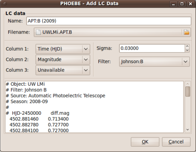
4.2 Passbands 12
not enforce that these names be unique, it is good practice to keep them
short and informative. An example may be APT:B (2009) for a light curve
acquired on the Automated Photoelectric Telescope (APT) in Johnson B
band in 2009. Provide the passband name in the Name field. If you omit
the name, a default will be applied, which is in the form filter-set:filter,
i.e. Johnson:B.
Next, select the corresponding file that contains the data by clicking on
the Filename selection button. This will open the dialog window and allow
you to browse to the location of your input file. Make sure that the file format
conforms to the specifications provided in §4.1. Note that the filenames are
stored with their complete paths, so they may reside anywhere on the disk.
Once a filename is selected, its contents will be previewed in the white space
below.
From the drop-down boxes assign input file columns: Time (HJD) or
Phase for the first column, Flux or Magnitude for the second column, and
Standard weight,Standard deviation or Unavailable for the third col-
umn. If observed data are radial velocities, the second column can be either
aPrimary RV or a Secondary RV in km/s.
Next, select an appropriate value for the standard deviation Sigma of
the observed curve. If the third column provides Standard weight or is
Unavailable, set the value of Sigma to the estimated root mean square (rms)
value of the data-set. It is not crucial to get this value completely right, it
4.2 Passbands 13
suffices to get a right order of magnitude for the first cut at the solution.
If, on the other hand, the third column provides Standard deviation, then
you should set the value of Sigma to 1.0 – otherwise you would be weighting
data points twice in that data-set.
Finally, select a filter according to the discussion in §4.2. Clicking on OK
will add the curve to the list of curves in the Data tab.
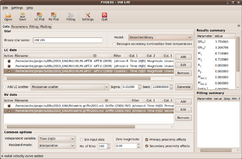
Continuing with our UW LMi example, add B,Vand IClight curves
acquired with APT, and primary and secondary radial velocities by Griffin
(2001) The RV data-set in this manual will be switched to Asiago observations
as soon as I finish reducing them since they’re ours and Griffin’s aren’t.
Once you are done with adding the data, there are two important details:
setting the Zero magnitude and setting the independent variable.
PHOEBE differs from other modeling codes in the treatment of light curves
that it uses a single zero magnitude for all passbands. This insures that the
color index of calibrated light curves is preserved and that both temperatures
of the binary components may be determined simultaneously. We will talk
about color constraining in detail in later sections.
After inspecting the light curve file contents, you can see that the quarter-
phase magnitudes of the three light curves are ∼0.7, ∼0.5 and ∼0.3 for
B,Vand ICpassbands, respectively. Based on this, you should set the zero
4.2 Passbands 14
magnitude to be close to the dimmest quarter-phase magnitude, thus 0.7.
Again, you do not need to worry on getting this value to match observations
perfectly; an order of magnitude is perfectly sufficient and we set it here to
0.0.
All computations in PHOEBE can be done either in time space or in phase
space. If your ephemeris changes (i.e. dP/dt or dω/dt are not 0), then you
must perform your computation in time space. This is also the case if you
want to fit any time dependent parameter. Otherwise you may perform
all calculations in phase space, which is numerically more efficient, but the
difference on modern computers is negligible. A rule of thumb is: if your
data are in time space, do computations in time space; if your data are in
phase space or mixed, do computations in phase space. Set the Independent
variable parameter accordingly.
The defaults on other parameters in the Data tab are usually sound. In
simulations it is sometimes useful to add synthetic scatter to model light
curves; this can be achieved by checking the Add LC scatter switch. The
scatter can be randomly sampled from the Poisson distribution (scaled with
the square root of the flux; this is the default and is appropriate for most
cases), from the uniform distribution (option None), or from the low light level
distribution (scaled linearly with flux; this is appropriate for faint sources).
The absolute size of scatter is governed by the parameter Sigma, while the
seed for the random number generator, if exact repeatability is desired, is set
by Seed.
The Passband mode parameter is not used in version 0.32; it pertains
to the manipulation of synthetic spectra and their multiplication with pass-
band transmission functions. It will be relevant once on-the-fly passband
integration is implemented.
Data may be binned; this may be desireable when the number of data
points per light curve is very large, i.e. 10,000 or more. In that case it might
prove useful to do most of the fitting on binned light curves and revert to a
much more time-expensive computation on full data-sets once the model is
close to the solution.
Finally, the radial velocity proximity effects for the primary and the sec-
ondary star are turned on by default, and can be turned off by unchecking
the Primary and Secondary proximity effects checkboxes.
Once you are done setting the data, you may save the current setup into
a parameter file. You do this by clicking on the Save button or selecting the
option from the File menu. By convention, PHOEBE parameter files are given
the extension .phoebe or .pho.
4.3 Data weighting 15
—————————–
It is a good practice to use the panel RV plot or LC plot to display each
data set just entered to be sure that it is what you want and that PHOEBE
reads it correctly.
4.3 Data weighting
PHOEBE supports three types of weights.
Intrinsic weights. As a measure of per-observation precision, each data
point can have an intrinsic weight attributed to it. For Ndata points
there will be Nintrinsic weights, which may be (optionally) supplied
in the third column of the input file. These weights can be expressed
either in terms of standard weight or in terms of standard deviation.
In the case of standard weight, the squares of the residuals are multi-
plied by the respective standard weights (cf. Eq. 1). Keep in mind that
their absolute scaling bears no significance on minimization: it will only
make the final cost function appear larger or smaller. This means that,
if all individual weights across all passbands are multiplied by the same
constant, the solution will be exactly the same. However, the relative
scaling across passbands is very significant: if individual weights of a
single curve were rescaled by a given constant, that passband would
either gain or loose the relative weight in comparison to other curves.
You must thus insure that all individual weights across all passbands
are scaled uniformly.
In the case of standard deviation, the squares of the residuals are di-
vided by the square of respective standard deviations (cf. Eq. 2). Every
data point now has a measure of precision that is directly comparable
to all other data points across all other passbands. Since standard devi-
ation will by typically provided in magnitudes, PHOEBE transforms σm
to σf; this is a non-symmetric transformation (σf+6=σf−) and PHOEBE
uses a conservative approach of selecting the larger of the two.
Passband-dependent weights. Every light and radial velocity curve has a
corresponding precision that is typically expressed in terms of standard
deviation (or r.m.s.). Each curve should thus be weighted by its relative
precision. If the intrinsic weights are given in terms of standard weight,
a passband-dependent weight of that curve will then simply be the
inverse square of its standard deviation, wp= 1/σ2
p. If, however, the
intrinsic weights are given in terms of standard deviation, then these

4.3 Data weighting 16
observations are already weighted in the absolute sense and applying
a passband-dependent weight would cause those points to be weighted
twice. That is why, for wigiven in terms of standard deviation, wp
(and thus σp) should be set to 1.
Level-dependent weights. Both photometric and spectroscopic data ac-
quisition is essentially photon counting, with a reasonably well under-
stood underlying statistics of how the noise scales with the light level.
In a Poisson regime (i.e. shot noise), the noise is proportional to the
square root of the flux: N∝√f. The S/N ratio thus increases with
the square root of the increasing flux, but so does the resulting scat-
ter; in turn, the level-dependent weight is inversely proportional to flux:
w∝f−1. In a low light level regime (i.e. scintillation noise), the noise is
linearly proportional to flux; the S/N ratio is constant with the increas-
ing flux, so the resulting scatter increases linearly. The level-dependent
weight in this regime is thus proportional to the inverse square of the
flux: w∝f−2. If the data are dominated by sources of scatter other
than those governed by the counting statistics (i.e. detector noise) and
are thus largely independent of the light level, the S/N ratio will then
increase linearly with the increasing flux, implying that the noise is con-
stant and there should be no level-dependent weighting applied. Radial
velocity observations are a most notable example of this regime; that
is why level-dependent weighting applies only to light curves.
The cost function of the fit that takes all three sources of noise into
account is expressed as:
χ2=X
p
1
σ2
p
Np
X
i=1
wi(fi−si)2
fR
i
,(1)
where index pruns over all available passbands, index iruns over Npobserva-
tions for p-th passband, wiare standard weights, fiand siare observed and
calculated fluxes, respectively, and Ris the level-dependent regime power:
R= 0 for no level-dependent weighting, R= 1 for Poisson noise, and R= 2
for low light noise. If intrinsic weights are given in terms of standard devia-
tion σi, Eq. (1) becomes:
χ2=X
p
1
σ∗
p2
Np
X
i=1
(fi−si)2
σ2
ifR
i
,(2)
Note that, as mentioned above, σiassume the role of passband weighting
as well, and σ∗
pneed to be set to 1. It may sometimes be desireable to
subjectively increase or decrease the influence of any given curve in the total
4.4 Propagating formal errors 17
value of χ2; this is achieved by setting σ∗
pto a value different from 1: larger
for less relative weight and smaller for more relative weight. That is the
reason why we do not omit the term with σ∗
pin Eq. (2). In particular,
σ∗
pshould be almost exclusively 1 for all photometric curves, but it may be
sometimes tweaked slightly for the radial velocity curves so that their relative
contribution is similar to those of light curves.
PHOEBE provides four important values in the Statistics summary of the
Fitting tab for each passband:
Unweighted residuals: Pi(fi−si)2
Intrinsically weighted residuals: Piwi(fi−si)2
Passband weighted residuals: 1/σ2
pPiwi(fi−si)2
Fully weighted residuals: 1/σ2
pPiwi(fi−si)2/fR
i
The cost function that is used to drive the minimizer is a sum of fully
weighted residuals and is displayed in the Fitting tab.
4.4 Propagating formal errors
When modeling eclipsing binary light and radial velocity curves simultane-
ously, it is not always clear how to proceed with computing formal errors
of the computed parameters such as stellar masses and radii. While we are
working on fundamentally changing the approach that is currently used to
compute formal errors (DC covariances will be replaced by Bayesian infer-
ence), we present here what seems to be best practice with the currently
available modeling software. Since each eclipsing binary has a unique pa-
rameter space, with characteristic parameter correlations and degeneracy,
your mileage may vary when following this ”recipe”.
TODO: Discuss LC-dominated and RV-dominated solutions
Computing formal errors for masses and radii basically boils down to
properly propagating formal errors of adjusted parameters. Propagation can
either be done the classical way (by propagating absolute or relative errors
as appropriate – and you’ll grow old trying to do this) or by evaluating a
log of the expression, differentiating it, and approximating σp≈ |dp|for all
parameters p. Absolute value in |dp|assures that formal errors accumulate.
Note that this is the most conservative approach, which can often be replaced
with summing the squares of standard deviations rather than adding them
linearly.
For masses we simply use Kepler’s 3rd law, while for the radii we need

4.4 Propagating formal errors 18
to use the expression for the generalized surface potential (Wilson 1979) for
elliptical orbits and asynchronous rotation:
Ω = 1
R+q1
[R2+D2−2RλD]1/2−λR
D2+1
2F2(1 + q)R2(1 −ν2),(3)
where λand νare direction cosines, Dis instantaneous separation of the
two components, Ris the fractional radius (relative to the semi-major axis),
q=M2/M1is the mass ratio, and Fis synchronicity parameter.
TODO: Discuss the determination of formal errors from the
covariance matrix
Once you have a final solution at hand, formal errors should be computed
by following these steps.
1. Compute asin i;
2. using only RV curves, set i= 90◦, set a=x, and adjust the following
parameters: a,q,vγ, ∆Φ, eand ω. Note that the fitted parameter a
is a proxy to asin i. Record formal errors without adopting adjusted
values of parameters. This way you should have obtained σasin i,σq
and σvγ; discard formal errors of the remaining parameters for now,
as they were only used to account for parameter correlations. Since
light curves were not used, these errors have likely been overestimated
anyway.
3. Set the semi-major axis and inclination back to their original values.
4. Using a full set of available light and RV curves, adjust all parameters
that have been varied (i.e. not assumed or derived from the outside,
i.e. spectroscopy) but omitting a,qand vγ. Once the convergence is
reached, record the formal errors of the adjusted parameters. Again,
do not adopt the corrected values.
5. Take σasin ifrom the RV fit and σifrom the simultaneous fit and com-
pute σa:
σa=σasin i
sin i+acos i σi
sin i(4)
6. Compute radii by the Newton-Raphson method (or simply trust PHOEBE
to do this for you). Since the shape of a star is fully determined by
the surface potential Ω, Eq. (3) has to be iteratively inverted to obtain
the radius Rfor the given λand ν. This is most easily achieved by
expressing the potential at the star’s pole (λ= 0, ν = 1):
Ω = 1
Rpole
+q
[D2+R2
pole]1/2.(5)

4.4 Propagating formal errors 19
Asserting that Ω is constant over the surface of the star yields:
1
R+q1
[R2+D2−2RλD]1/2−Rλ
D2+1
2F2(1 + q)R2(1 −ν2) =
=1
Rpole
+q 1
[D2+R2
pole]1/2!.(6)
Solving this equation iteratively for Rgiven any λand νdetermines
the local fractional radius of the star.
7. Use σa,σPand σqto compute formal errors of individual masses:
M1=4π2a3
GP 2
1
1 + q;M2=4π2a3
GP 2
q
1 + q;
σM1=M13σa
a+ 2σP
P+σq
q+ 1; (7)
σM2=M23σa
a+ 2σP
P+σq
q(q+ 1).(8)
8. Use σΩ,σq,σeand σFto compute formal errors of fractional radii:
σR=
1
A1
σΩ+
A2
A1
σq+
A3
A1
σe+
A4
A1
σF,(9)
where:
A1=−1
R2−q(R+e−1)
[R2+ (1 −e)2−2R(1 −e)]3/2−q
(1 −e)2+F2(1 + q)R,
A2=1
[R2+ (1 −e)2−2R(1 −e)]1/2−R
(1 −e)2+1
2F2R2,
A3=−q(R+e−1)
[R2+ (1 −e)2−2R(1 −e)]3/2−2qR
(1 −e)3,
A4=F(1 + q)R2.(10)
Here we assumed the point radius, i.e. λ= 1, ν= 0, and periastron
separation D= 1 −e, to get the largest estimate on σR.
5 SOLVING THE INVERSE TASK IN PHOEBE 20
5 SOLVING THE INVERSE TASK IN PHOEBE
5.1 DIFFERENTIAL CORRECTIONS
The choice of differential correction methods of consecutive iterations of the
chosen physical parameters is the built-in initial choice in PHOEBE. Before
running it, think a bit about the range of inidividual parameters and their
steps, defined in panel PARAMETERS and modify them if necessary to
suite to your task. As explained by Prˇsa and Zwitter (2006), convergency
of primary flux levels from the beginning along with other parameters leads
to a very slow oscillatory convergence. It is therefore very desirable to go
first to PARAMETERS/LUMINOSITIES and use the option CALCULATE
step by step for each data subset. Only then start the convergency of all
desired parameters using the top panel FITTING. Andrej, please explain
how to decide that convergency was reached after some number of iterations
and provide also other advice on the strategy of the solution.
5.2 NELDER AND MEAD SIMPLEX
Andrej, just questions here: Please, explain whether one should ask for cal-
culation of the cost function right before running the fitting in the internal
panel FITTING. Again - when the convergency was reached? Why the cost
function is different from that calculated by differential corrections? How to
prevent the program to run out of permissible range?
5.3 USING THE SCRIPTER
Andrej, it would be great to put here a few examples of batches of scripter
commands for some typical calculations. If fixed format is needed soemwhere,
you can use the sample Table attached below after ‘end of document’ com-
mand.
6 OUTPUT OF RESULTS
1. Note that various pieces of information about the results are scattered
over various panels. Thus, for instance all physical epochs for elliptical
orbit are listed in panel PARAMETERS/ORBIT.

REFERENCES 21
2. Note that masses, radii, log g and bolometric magnitudes are only
upgraded when you run LC PLOT. It is so because only this plot
actives calculation with the LC program.
3. In panel Fitting one gets lines with information about individual data
sets. The ”Relative weight” column has been changed to ”Weighted
sum of residuals”. The values reported there are:
1
σ2
iX
i
wiwp(ci)(oi−ci)2(11)
where σiis the passband sigma, wiare individual weights, and wp(ci)
are level-dependent weights.
4. Be aware that phasing the light curves in PHOEBE does not take apsi-
dal motion into account, i.e. only dP/dtis considered in the calculation
of phases, while dω/dtis not. The reason is that the apsidal motion is
actually changing the shape of the light and RV curves and the phase
separation of the primary and secondary eclipses. Therefore, if one
wants to see how good the fit is, the only sensible option is to display
residuals vs. time (HJD).
It would be great to include into this manual a table with individual parame-
ters which can be converged with indication in which units they are treated.
Important especially for paramaters such a period derivative etc. Would it be
too complicated to have ωand ˙ωin degrees and degs. per day, respectively, on
the input and output as used in the vast majority of publications? Could op-
tionally be the luminosities in the output be normalized i.e. L1+L2+L3=1?
For larger number of datasets one has to do lot of calculations manually
and the advantage of these relative luminosities is that you see immediately
whether they are changing in a logical way with wavelength.
References
Castelli, F. and Kurucz, R. L.: 2004, ArXiv Astrophysics e-prints
van Hamme, W.: 1993, AJ 106, 2096
Wilson, R. E. and Devinney, E. J.: 1971, ApJ 166, 605