[P] Programming Manual
User Manual:
Open the PDF directly: View PDF ![]() .
.
Page Count: 631 [warning: Documents this large are best viewed by clicking the View PDF Link!]
- Contents
- [IG] Installation Guide
- Simple installation
- Installing Stata for Windows
- Installing Stata for Mac
- Installing Stata for Unix
- Installation overview
- Find your installation DVD and paper license
- Obtain superuser access
- Create a directory for Stata
- Upgrading
- Install Stata
- Initialize the license
- Set the message of the day (optional)
- Verify that Stata is working
- Modify shell start-up script
- Update Stata if necessary
- Starting Stata
- Exiting Stata
- Troubleshooting Unix installation
- Troubleshooting Unix start-up
- Stata(console) starts but Stata(GUI) does not
- Platforms and flavors
- Documentation
- [GS] Getting Started
- [GSM] Mac
- Contents
- 1 Introducing Stata---sample session
- 2 The Stata user interface
- 3 Using the Viewer
- The Viewer's purpose
- Viewer buttons
- Viewer's function
- Viewing local text files, including SMCL files
- Viewing remote files over the Internet
- Navigating within the Viewer
- Printing
- Tabs in the Viewer
- Right-clicking on the Viewer window
- Searching for help in the Viewer
- Commands in the Viewer
- Using the Viewer from the Command window
- 4 Getting help
- 5 Opening and saving Stata datasets
- 6 Using the Data Editor
- 7 Using the Variables Manager
- 8 Importing data
- 9 Labeling data
- 10 Listing data and basic command syntax
- 11 Creating new variables
- 12 Deleting variables and observations
- 13 Using the Do-file Editor---automating Stata
- 14 Graphing data
- 15 Editing graphs
- 16 Saving and printing results by using logs
- 17 Setting font and window preferences
- 18 Learning more about Stata
- 19 Updating and extending Stata---Internet functionality
- A Troubleshooting Stata
- B Advanced Stata usage
- C More on Stata for Mac
- Subject index
- [GSU] Unix
- Contents
- 1 Introducing Stata---sample session
- 2 The Stata user interface
- 3 Using the Viewer
- The Viewer in Stata(GUI)
- The Viewer's purpose
- Viewer buttons
- Viewer's function
- Viewing local text files, including SMCL files
- Viewing remote files over the Internet
- Navigating within the Viewer
- Printing
- Tabs in the Viewer
- Right-clicking on the Viewer window
- Searching for help in the Viewer
- Commands in the Viewer
- Using the Viewer from the Command window
- 4 Getting help
- 5 Opening and saving Stata datasets
- 6 Using the Data Editor
- 7 Using the Variables Manager
- 8 Importing data
- 9 Labeling data
- 10 Listing data and basic command syntax
- 11 Creating new variables
- 12 Deleting variables and observations
- 13 Using the Do-file Editor---automating Stata
- 14 Graphing data
- 15 Editing graphs
- 16 Saving and printing results by using logs
- 17 Setting font and window preferences
- 18 Learning more about Stata
- 19 Updating and extending Stata---Internet functionality
- A Troubleshooting Stata
- B Advanced Stata usage
- C Stata manual pages for Unix
- conren
- stata
- Subject index
- [GSW] Windows
- Contents
- 1 Introducing Stata---sample session
- 2 The Stata user interface
- 3 Using the Viewer
- The Viewer's purpose
- Viewer buttons
- Viewer's function
- Viewing local text files, including SMCL files
- Viewing remote files over the Internet
- Navigating within the Viewer
- Printing
- Tabs in the Viewer
- Right-clicking on the Viewer window
- Searching for help in the Viewer
- Commands in the Viewer
- Using the Viewer from the Command window
- 4 Getting help
- 5 Opening and saving Stata datasets
- 6 Using the Data Editor
- 7 Using the Variables Manager
- 8 Importing data
- 9 Labeling data
- 10 Listing data and basic command syntax
- 11 Creating new variables
- 12 Deleting variables and observations
- 13 Using the Do-file Editor---automating Stata
- 14 Graphing data
- 15 Editing graphs
- 16 Saving and printing results by using logs
- 17 Setting font and window preferences
- 18 Learning more about Stata
- 19 Updating and extending Stata---Internet functionality
- A Troubleshooting Stata
- B Advanced Stata usage
- C More on Stata for Windows
- Subject index
- [GSM] Mac
- [U] User's Guide
- Contents
- Stata basics
- Elements of Stata
- 11 Language syntax
- 12 Data
- 13 Functions and expressions
- 13.1 Overview
- 13.2 Operators
- 13.3 Functions
- 13.4 System variables (_variables)
- 13.5 Accessing coefficients and standard errors
- 13.6 Accessing results from Stata commands
- 13.7 Explicit subscripting
- 13.8 Using the Expression Builder
- 13.9 Indicator values for levels of factor variables
- 13.10 Time-series operators
- 13.11 Label values
- 13.12 Precision and problems therein
- 13.13 References
- 14 Matrix expressions
- 14.1 Overview
- 14.2 Row and column names
- 14.3 Vectors and scalars
- 14.4 Inputting matrices by hand
- 14.5 Accessing matrices created by Stata commands
- 14.6 Creating matrices by accumulating data
- 14.7 Matrix operators
- 14.8 Matrix functions
- 14.9 Subscripting
- 14.10 Using matrices in scalar expressions
- 14.11 Reference
- 15 Saving and printing output---log files
- 16 Do-files
- 17 Ado-files
- 17.1 Description
- 17.2 What is an ado-file?
- 17.3 How can I tell if a command is built in or an ado-file?
- 17.4 How can I look at an ado-file?
- 17.5 Where does Stata look for ado-files?
- 17.6 How do I install an addition?
- 17.7 How do I add my own ado-files?
- 17.8 How do I install official updates?
- 17.9 How do I install updates to user-written additions?
- 17.10 Reference
- 18 Programming Stata
- 18.1 Description
- 18.2 Relationship between a program and a do-file
- 18.3 Macros
- 18.4 Program arguments
- 18.5 Scalars and matrices
- 18.6 Temporarily destroying the data in memory
- 18.7 Temporary objects
- 18.8 Accessing results calculated by other programs
- 18.9 Accessing results calculated by estimation commands
- 18.10 Storing results
- 18.11 Ado-files
- 18.12 Tools for interacting with programs outside Stata and with other languages
- 18.13 A compendium of useful commands for programmers
- 18.14 References
- 19 Immediate commands
- 20 Estimation and postestimation commands
- 20.1 All estimation commands work the same way
- 20.2 Standard syntax
- 20.3 Replaying prior results
- 20.4 Cataloging estimation results
- 20.5 Saving estimation results
- 20.6 Specifying the estimation subsample
- 20.7 Specifying the width of confidence intervals
- 20.8 Formatting the coefficient table
- 20.9 Obtaining the variance--covariance matrix
- 20.10 Obtaining predicted values
- 20.11 Accessing estimated coefficients
- 20.12 Performing hypothesis tests on the coefficients
- 20.13 Obtaining linear combinations of coefficients
- 20.14 Obtaining nonlinear combinations of coefficients
- 20.15 Obtaining marginal means, adjusted predictions, and predictive margins
- 20.16 Obtaining conditional and average marginal effects
- 20.17 Obtaining pairwise comparisons
- 20.18 Obtaining contrasts, tests of interactions, and main effects
- 20.19 Graphing margins, marginal effects, and contrasts
- 20.20 Dynamic forecasts and simulations
- 20.21 Obtaining robust variance estimates
- 20.22 Obtaining scores
- 20.23 Weighted estimation
- 20.24 A list of postestimation commands
- 20.25 References
- Advice
- 21 Entering and importing data
- 22 Combining datasets
- 23 Working with strings
- 24 Working with dates and times
- 25 Working with categorical data and factor variables
- 26 Overview of Stata estimation commands
- 26.1 Introduction
- 26.2 Means, proportions, and related statistics
- 26.3 Linear regression with simple error structures
- 26.4 Structural equation modeling (SEM)
- 26.5 ANOVA, ANCOVA, MANOVA, and MANCOVA
- 26.6 Generalized linear models
- 26.7 Binary-outcome qualitative dependent-variable models
- 26.8 ROC analysis
- 26.9 Conditional logistic regression
- 26.10 Fractional-outcome dependent-variable models
- 26.11 Multiple-outcome qualitative dependent-variable models
- 26.12 Item response theory
- 26.13 Count dependent-variable models
- 26.14 Exact estimators
- 26.15 Linear regression with heteroskedastic errors
- 26.16 Stochastic frontier models
- 26.17 Regression with systems of equations
- 26.18 Models with endogenous sample selection
- 26.19 Models with time-series data
- 26.20 Panel-data models
- 26.21 Multilevel mixed-effects models
- 26.22 Survival-time (failure-time) models
- 26.23 Treatment-effect models
- 26.24 Generalized method of moments (GMM)
- 26.25 Estimation with correlated errors
- 26.26 Survey data
- 26.27 Multiple imputation
- 26.28 Multivariate and cluster analysis
- 26.29 Pharmacokinetic data
- 26.30 Specification search tools
- 26.31 Power and sample-size analysis
- 26.32 Bayesian analysis
- 26.33 Obtaining new estimation commands
- 26.34 References
- 27 Commands everyone should know
- 28 Using the Internet to keep up to date
- [BAYES] Bayesian Analysis
- Contents
- intro
- Description
- Remarks and examples
- References
- Also see
- bayes
- bayesmh
- Description
- Quick start
- Menu
- Syntax
- Options
- Remarks and examples
- Using bayesmh
- Setting up a posterior model
- Specifying MCMC sampling procedure
- Summarizing and reporting results
- Convergence of MCMC
- Getting started examples
- Logistic regression model: a case of nonidentifiable parameters
- Ordered probit regression
- Beta-binomial model
- Multivariate regression
- Panel-data and multilevel models
- Bayesian analysis of change-point problem
- Bioequivalence in a crossover trial
- Random-effects meta-analysis of clinical trials
- Item response theory
- Stored results
- Methods and formulas
- References
- Also see
- bayesmh evaluators
- bayesmh postestimation
- bayesgraph
- bayesstats
- bayesstats ess
- bayesstats ic
- bayesstats summary
- bayestest
- bayestest interval
- bayestest model
- set clevel
- Glossary
- [D] Data Management
- Contents
- intro
- data management
- append
- assert
- bcal
- by
- cd
- cf
- changeeol
- checksum
- clear
- clonevar
- codebook
- collapse
- compare
- compress
- contract
- copy
- corr2data
- count
- cross
- data types
- datasignature
- datetime
- Description
- Syntax
- Types of dates and their human readable forms (HRFs)
- Stata internal form (SIF)
- HRF-to-SIF conversion functions
- Displaying SIFs in HRF
- Building SIFs from components
- SIF-to-SIF conversion
- Extracting time-of-day components from SIFs
- Extracting date components from SIFs
- Conveniently typing SIF values
- Obtaining and working with durations
- Using dates and times from other software
- Remarks and examples
- References
- Also see
- datetime business calendars
- datetime business calendars creation
- Description
- Syntax
- Remarks and examples
- Introduction
- Concepts
- The preliminary commands
- The omit commands: from/to and if
- The omit commands: and
- The omit commands: omit date
- The omit commands: omit dayofweek
- The omit commands: omit dowinmonth
- Creating stbcal-files with bcal create
- Where to place stbcal-files
- How to debug stbcal-files
- Ideas for calendars that may not occur to you
- Also see
- datetime display formats
- datetime translation
- Description
- Syntax
- Remarks and examples
- Introduction
- Specifying the mask
- How the HRF-to-SIF functions interpret the mask
- Working with two-digit years
- Working with incomplete dates and times
- Translating run-together dates, such as 20060125
- Valid times
- The clock() and Clock() functions
- Why there are two SIF datetime encodings
- Advice on using datetime/c and datetime/C
- Determining when leap seconds occurred
- The date() function
- The other translation functions
- Also see
- describe
- destring
- dir
- drawnorm
- drop
- ds
- duplicates
- edit
- egen
- encode
- erase
- expand
- expandcl
- export
- filefilter
- fillin
- format
- generate
- gsort
- hexdump
- icd
- icd9
- icd10
- import
- import delimited
- import excel
- import haver
- import sasxport
- infile (fixed format)
- infile (free format)
- infix (fixed format)
- input
- insobs
- inspect
- ipolate
- isid
- joinby
- label
- label language
- labelbook
- list
- lookfor
- memory
- merge
- missing values
- mkdir
- mvencode
- notes
- obs
- odbc
- order
- outfile
- pctile
- putmata
- range
- recast
- recode
- rename
- rename group
- reshape
- Description
- Quick start
- Menu
- Syntax
- Options
- Remarks and examples
- Description of basic syntax
- Wide and long data forms
- Avoiding and correcting mistakes
- reshape long and reshape wide without arguments
- Missing variables
- Advanced issues with basic syntax: i()
- Advanced issues with basic syntax: j()
- Advanced issues with basic syntax: xij
- Advanced issues with basic syntax: String identifiers for j()
- Advanced issues with basic syntax: Second-level nesting
- Description of advanced syntax
- Stored results
- Acknowledgment
- References
- Also see
- rmdir
- sample
- save
- separate
- shell
- snapshot
- sort
- split
- stack
- statsby
- sysuse
- type
- unicode
- unicode collator
- unicode convertfile
- unicode encoding
- unicode locale
- unicode translate
- use
- varmanage
- webuse
- xmlsave
- xpose
- zipfile
- [FN] Functions
- Contents
- intro
- Functions by category
- Functions by name
- Date and time functions
- Contents
- Functions
- bofd()
- Cdhms()
- Chms()
- Clock()
- clock()
- Cmdyhms()
- Cofc()
- cofC()
- Cofd()
- cofd()
- daily()
- date()
- day()
- dhms()
- dofb()
- dofC()
- dofc()
- dofh()
- dofm()
- dofq()
- dofw()
- dofy()
- dow()
- doy()
- halfyear()
- halfyearly()
- hh()
- hhC()
- hms()
- hofd()
- hours()
- mdy()
- mdyhms()
- minutes()
- mm()
- mmC()
- mofd()
- month()
- monthly()
- msofhours()
- msofminutes()
- msofseconds()
- qofd()
- quarter()
- quarterly()
- seconds()
- ss()
- ssC()
- tC()
- tc()
- td()
- th()
- tm()
- tq()
- tw()
- week()
- weekly()
- wofd()
- year()
- yearly()
- yh()
- ym()
- yofd()
- yq()
- yw()
- Also see
- Mathematical functions
- Matrix functions
- Programming functions
- Contents
- Functions
- autocode()
- byteorder()
- c()
- _caller()
- chop()
- clip()
- cond()
- e()
- e(sample)
- epsdouble()
- epsfloat()
- fileexists()
- fileread()
- filereaderror()
- filewrite()
- float()
- fmtwidth()
- has_eprop()
- inlist()
- inrange()
- irecode()
- matrix()
- maxbyte()
- maxdouble()
- maxfloat()
- maxint()
- maxlong()
- mi()
- minbyte()
- mindouble()
- minfloat()
- minint()
- minlong()
- missing()
- r()
- recode()
- replay()
- return()
- s()
- scalar()
- smallestdouble()
- References
- Also see
- Random-number functions
- Selecting time-span functions
- Statistical functions
- Contents
- Functions
- Beta and noncentral beta distributions
- betaden()
- ibeta()
- ibetatail()
- invibeta()
- invibetatail()
- nbetaden()
- nibeta()
- invnibeta()
- Binomial distributions
- binomialp()
- binomial()
- binomialtail()
- invbinomial()
- invbinomialtail()
- Chi-squared and noncentral chi-squared distributions
- chi2den()
- chi2()
- chi2tail()
- invchi2()
- invchi2tail()
- nchi2den()
- nchi2()
- nchi2tail()
- invnchi2()
- invnchi2tail()
- npnchi2()
- Dunnett's multiple range distributions
- dunnettprob()
- invdunnettprob()
- Exponential distributions
- exponentialden()
- exponential()
- exponentialtail()
- invexponential()
- invexponentialtail()
- F and noncentral F distributions
- Fden()
- F()
- Ftail()
- invF()
- invFtail()
- nFden()
- nF()
- nFtail()
- invnF()
- invnFtail()
- npnF()
- Gamma and inverse gamma distributions
- gammaden()
- gammap()
- gammaptail()
- invgammap()
- invgammaptail()
- dgammapda()
- dgammapdada()
- dgammapdadx()
- dgammapdx()
- dgammapdxdx()
- lnigammaden()
- Hypergeometric distributions
- hypergeometricp()
- hypergeometric()
- Inverse Gaussian distributions
- igaussianden()
- igaussian()
- igaussiantail()
- invigaussian()
- invigaussiantail()
- lnigaussianden()
- Logistic distributions
- logisticden(x)
- logisticden(sx)
- logisticden()
- logisticden(msx)
- logistic()
- logistic(x)
- logistic(sx)
- logistic(msx)
- logistictail()
- logistictail(x)
- logistictail(sx)
- logistictail(msx)
- invlogistic()
- invlogistic(p)
- invlogistic(sp)
- invlogistic(msp)
- invlogistictail()
- invlogistictail(p)
- invlogistictail(sp)
- invlogistictail(msp)
- Negative binomial distributions
- nbinomialp()
- nbinomial()
- nbinomialtail()
- invnbinomial()
- invnbinomialtail()
- Normal (Gaussian), log of the normal, binormal, and multivariate normal distributions
- normalden()
- normalden(xs)
- normalden(xms)
- normal()
- invnormal()
- lnnormalden()
- lnnormalden(xs)
- lnnormalden(xms)
- lnnormal()
- binormal()
- lnmvnormalden()
- Poisson distributions
- poissonp()
- poisson()
- poissontail()
- invpoisson()
- invpoissontail()
- Student's t and noncentral Student's t distributions
- tden()
- t()
- ttail()
- invt()
- invttail()
- invnt()
- invnttail()
- ntden()
- nt()
- nttail()
- npnt()
- Tukey's Studentized range distributions
- tukeyprob()
- invtukeyprob()
- Weibull distributions
- weibullden()
- weibullden(abx)
- weibullden(abgx)
- weibull()
- weibull(abx)
- weibull(abgx)
- weibulltail()
- weibulltail(abx)
- weibulltail(abgx)
- invweibull()
- invweibull(abp)
- invweibull(abgp)
- invweibulltail()
- invweibulltail(abp)
- invweibulltail(abgp)
- Weibull (proportional hazards) distributions
- weibullphden()
- weibullphden(abx)
- weibullphden(abgx)
- weibullph()
- weibullph(abx)
- weibullph(abgx)
- weibullphtail()
- weibullphtail(abx)
- weibullphtail(abgx)
- invweibullph()
- invweibullph(abp)
- invweibullph(abgp)
- invweibullphtail()
- invweibullphtail(abp)
- invweibullphtail(abgp)
- Wishart and inverse Wishart distributions
- lnwishartden()
- lniwishartden()
- References
- Also see
- String functions
- Contents
- Functions
- abbrev()
- char()
- uchar()
- collatorlocale()
- collatorversion()
- indexnot()
- plural()
- real()
- regexm()
- regexr()
- regexs()
- ustrregexm()
- ustrregexrf()
- ustrregexra()
- ustrregexs()
- soundex()
- soundex_nara()
- strcat()
- strdup()
- string()
- string(ns)
- stritrim()
- strlen()
- ustrlen()
- udstrlen()
- strlower()
- ustrlower()
- strltrim()
- ustrltrim()
- strmatch()
- strofreal()
- strofreal(ns)
- strpos()
- ustrpos()
- strproper()
- ustrtitle()
- strreverse()
- ustrreverse()
- strrpos()
- ustrrpos()
- strrtrim()
- ustrrtrim()
- strtoname()
- ustrtoname()
- strtrim()
- ustrtrim()
- strupper()
- ustrupper()
- subinstr()
- usubinstr()
- subinword()
- substr()
- usubstr()
- udsubstr()
- tobytes()
- uisdigit()
- uisletter()
- ustrcompare()
- ustrcompareex()
- ustrfix()
- ustrfrom()
- ustrinvalidcnt()
- ustrleft()
- ustrnormalize()
- ustrright()
- ustrsortkey()
- ustrsortkeyex()
- ustrto()
- ustrtohex()
- ustrunescape()
- word()
- ustrword()
- wordbreaklocale()
- wordcount()
- ustrwordcount()
- References
- Also see
- Trigonometric functions
- [G] Graphics
- Contents
- Introduction
- Commands
- graph
- graph bar
- Description
- Quick start
- Menu
- Syntax
- Options
- Remarks and examples
- Introduction
- Examples of syntax
- Treatment of bars
- Treatment of data
- Obtaining frequencies
- Multiple bars (overlapping the bars)
- Controlling the text of the legend
- Multiple over()s (repeating the bars)
- Nested over()s
- Charts with many categories
- How bars are ordered
- Reordering the bars
- Putting the bars in a prespecified order
- Putting the bars in height order
- Putting the bars in a derived order
- Reordering the bars, example
- Use with by()
- Video example
- History
- References
- Also see
- graph box
- graph close
- graph combine
- graph copy
- graph describe
- graph dir
- graph display
- graph dot
- graph drop
- graph export
- graph manipulation
- graph matrix
- graph other
- graph pie
- graph play
- graph print
- graph query
- graph rename
- graph replay
- graph save
- graph set
- graph twoway
- graph twoway area
- graph twoway bar
- graph twoway connected
- graph twoway contour
- graph twoway contourline
- graph twoway dot
- graph twoway dropline
- graph twoway fpfit
- graph twoway fpfitci
- graph twoway function
- graph twoway histogram
- graph twoway kdensity
- graph twoway lfit
- graph twoway lfitci
- graph twoway line
- graph twoway lowess
- graph twoway lpoly
- graph twoway lpolyci
- graph twoway mband
- graph twoway mspline
- graph twoway pcarrow
- graph twoway pcarrowi
- graph twoway pccapsym
- graph twoway pci
- graph twoway pcscatter
- graph twoway pcspike
- graph twoway qfit
- graph twoway qfitci
- graph twoway rarea
- graph twoway rbar
- graph twoway rcap
- graph twoway rcapsym
- graph twoway rconnected
- graph twoway rline
- graph twoway rscatter
- graph twoway rspike
- graph twoway scatter
- Description
- Quick start
- Menu
- Syntax
- Options
- Remarks and examples
- Typical use
- Scatter syntax
- The overall look for the graph
- The size and aspect ratio of the graph
- Titles
- Axis titles
- Axis labels and ticking
- Grid lines
- Added lines
- Axis range
- Log scales
- Multiple axes
- Markers
- Weighted markers
- Jittered markers
- Connected lines
- Graphs by groups
- Saving graphs
- Video example
- Appendix: Styles and composite styles
- References
- Also see
- graph twoway scatteri
- graph twoway spike
- graph twoway tsline
- graph use
- palette
- set graphics
- set printcolor
- set scheme
- Options
- added_line_options
- added_text_options
- addplot_option
- advanced_options
- area_options
- aspect_option
- axis_choice_options
- Description
- Syntax
- Options
- Remarks and examples
- Usual case: one set of axes
- Special case: multiple axes due to multiple scales
- yaxis(1) and xaxis(1) are the defaults
- Notation style is irrelevant
- yaxis() and xaxis() are plot options
- Specifying the other axes options with multiple axes
- Each plot may have at most one x scale and one y scale
- Special case: Multiple axes with a shared scale
- Reference
- Also see
- axis_label_options
- axis_options
- axis_scale_options
- axis_title_options
- barlook_options
- blabel_option
- by_option
- cat_axis_label_options
- cat_axis_line_options
- clegend_option
- cline_options
- connect_options
- eps_options
- fcline_options
- fitarea_options
- legend_options
- line_options
- marker_label_options
- marker_options
- name_option
- nodraw_option
- play_option
- png_options
- pr_options
- ps_options
- rcap_options
- region_options
- rspike_options
- saving_option
- scale_option
- scheme_option
- std_options
- textbox_options
- tif_options
- title_options
- twoway_options
- Styles/concepts/schemes
- addedlinestyle
- alignmentstyle
- anglestyle
- areastyle
- axisstyle
- bystyle
- clockposstyle
- colorstyle
- compassdirstyle
- concept: gph files
- concept: lines
- concept: repeated options
- connectstyle
- gridstyle
- intensitystyle
- justificationstyle
- legendstyle
- linepatternstyle
- linestyle
- linewidthstyle
- marginstyle
- markerlabelstyle
- markersizestyle
- markerstyle
- orientationstyle
- plotregionstyle
- pstyle
- relativesize
- ringposstyle
- schemes intro
- scheme economist
- scheme s1
- scheme s2
- scheme sj
- shadestyle
- stylelists
- symbolstyle
- text
- textboxstyle
- textsizestyle
- textstyle
- ticksetstyle
- tickstyle
- [IRT] Item Response Theory
- Contents
- irt
- Control Panel
- irt 1pl
- irt 1pl postestimation
- irt 2pl
- irt 2pl postestimation
- irt 3pl
- irt 3pl postestimation
- irt grm
- irt grm postestimation
- irt nrm
- irt nrm postestimation
- irt pcm
- irt pcm postestimation
- irt rsm
- irt rsm postestimation
- irt hybrid
- irt hybrid postestimation
- estat report
- irtgraph icc
- irtgraph tcc
- irtgraph iif
- irtgraph tif
- dif
- diflogistic
- difmh
- Glossary
- [M] Mata
- Contents
- Introduction to the Mata manual
- Introduction and advice
- intro
- ado
- first
- Description
- Remarks and examples
- Invoking Mata
- Using Mata
- Making mistakes: Interpreting error messages
- Working with real numbers, complex numbers, and strings
- Working with scalars, vectors, and matrices
- Working with functions
- Distinguishing real and complex values
- Working with matrix and scalar functions
- Performing element-by-element calculations: Colon operators
- Writing programs
- More functions
- Mata environment commands
- Exiting Mata
- Also see
- help
- how
- interactive
- Description
- Remarks and examples
- 1. Start in Stata; load the data
- 2. Create any time-series variables
- 3. Create a constant variable
- 4. Drop unnecessary variables
- 5. Drop observations with missing values
- 6. Put variables on roughly the same numeric scale
- 7. Enter Mata
- 8. Use Mata's st_view() function to access your data
- 9. Perform your matrix calculations
- Review
- Reference
- Also see
- LAPACK
- limits
- naming
- permutation
- returnedargs
- source
- tolerance
- Language definition
- intro
- break
- class
- Description
- Syntax
- Remarks and examples
- Notation and jargon
- Declaring and defining a class
- Saving classes in files
- Workflow recommendation
- When you need to recompile
- Obtaining instances of a class
- Constructors and destructors
- Setting member variable and member function exposure
- Making a member final
- Making a member static
- Virtual functions
- Referring to the current class using this
- Using super to access the parent's concept
- Casting back to a parent
- Accessing external functions from member functions
- Pointers to classes
- Also see
- comments
- continue
- declarations
- do
- errors
- exp
- for
- ftof
- goto
- if
- op_arith
- op_assignment
- op_colon
- op_conditional
- op_increment
- op_join
- op_kronecker
- op_logical
- op_range
- op_transpose
- optargs
- pointers
- pragma
- reswords
- return
- semicolons
- struct
- Description
- Syntax
- Remarks and examples
- Introduction
- Structures and functions must have different names
- Structure variables must be explicitly declared
- Declare structure variables to be scalars whenever possible
- Vectors and matrices of structures
- Structures of structures
- Pointers to structures
- Operators and functions for use with structure members
- Operators and functions for use with entire structures
- Listing structures
- Use of transmorphics as passthrus
- Saving compiled structure definitions
- Saving structure variables
- Reference
- Also see
- subscripts
- syntax
- version
- void
- while
- Commands for controlling Mata
- Categorical guide to functions
- Alphabetical index to functions
- intro
- abbrev()
- abs()
- adosubdir()
- all()
- args()
- asarray()
- AssociativeArray()
- ascii()
- uchar()
- assert()
- blockdiag()
- bufio()
- byteorder()
- C()
- c()
- callersversion()
- cat()
- chdir()
- cholesky()
- cholinv()
- cholsolve()
- comb()
- cond()
- conj()
- corr()
- cross()
- crossdev()
- cvpermute()
- date()
- deriv()
- designmatrix()
- det()
- _diag()
- diag()
- diag0cnt()
- diagonal()
- dir()
- direxists()
- direxternal()
- display()
- displayas()
- displayflush()
- Dmatrix()
- _docx*()
- dsign()
- e()
- editmissing()
- edittoint()
- edittozero()
- editvalue()
- eigensystem()
- eigensystemselect()
- eltype()
- epsilon()
- _equilrc()
- error()
- errprintf()
- exit()
- exp()
- factorial()
- favorspeed()
- ferrortext()
- fft()
- fileexists()
- _fillmissing()
- findexternal()
- findfile()
- floatround()
- fmtwidth()
- fopen()
- fullsvd()
- geigensystem()
- ghessenbergd()
- ghk()
- ghkfast()
- gschurd()
- halton()
- hash1()
- hessenbergd()
- Hilbert()
- I()
- inbase()
- indexnot()
- invorder()
- invsym()
- invtokens()
- isdiagonal()
- isfleeting()
- isreal()
- isrealvalues()
- issymmetric()
- isview()
- J()
- Kmatrix()
- lapack()
- liststruct()
- Lmatrix()
- logit()
- lowertriangle()
- lud()
- luinv()
- lusolve()
- makesymmetric()
- matexpsym()
- matpowersym()
- mean()
- mindouble()
- minindex()
- minmax()
- missing()
- missingof()
- mod()
- moptimize()
- Description
- Syntax
- Step 1: Initialization
- Step 2: Definition of maximization or minimization problem
- Step 3: Perform optimization or perform a single function evaluation
- Step 4: Post, display, or obtain results
- Utility functions for use in all steps
- Definition of M
- Setting the sample
- Specifying dependent variables
- Specifying independent variables
- Specifying constraints
- Specifying weights or survey data
- Specifying clusters and panels
- Specifying optimization technique
- Specifying initial values
- Performing one evaluation of the objective function
- Performing optimization of the objective function
- Tracing optimization
- Specifying convergence criteria
- Accessing results
- Stata evaluators
- Advanced functions
- Syntax of evaluators
- Syntax of type lf evaluators
- Syntax of type d evaluators
- Syntax of type lf* evaluators
- Syntax of type gf evaluators
- Syntax of type q evaluators
- Passing extra information to evaluators
- Utility functions
- Remarks and examples
- Conformability
- Diagnostics
- References
- Also see
- more()
- _negate()
- norm()
- normal()
- optimize()
- panelsetup()
- pathjoin()
- Pdf*()
- pinv()
- polyeval()
- printf()
- qrd()
- qrinv()
- qrsolve()
- quadcross()
- range()
- rank()
- Re()
- reldif()
- rows()
- rowshape()
- runiform()
- runningsum()
- schurd()
- select()
- setbreakintr()
- sign()
- sin()
- sizeof()
- solve_tol()
- solvelower()
- solvenl()
- sort()
- soundex()
- spline3()
- sqrt()
- st_addobs()
- st_addvar()
- st_data()
- st_dir()
- st_dropvar()
- st_global()
- st_isfmt()
- st_isname()
- st_local()
- st_macroexpand()
- st_matrix()
- st_numscalar()
- st_nvar()
- st_rclear()
- st_store()
- st_subview()
- st_tempname()
- st_tsrevar()
- st_updata()
- st_varformat()
- st_varindex()
- st_varname()
- st_varrename()
- st_vartype()
- st_view()
- st_viewvars()
- st_vlexists()
- stata()
- stataversion()
- strdup()
- strlen()
- ustrlen()
- udstrlen()
- strmatch()
- strofreal()
- strpos()
- ustrpos()
- strreverse()
- ustrreverse()
- strtoname()
- ustrtoname()
- strtoreal()
- strtrim()
- ustrtrim()
- strupper()
- ustrupper()
- subinstr()
- usubinstr()
- sublowertriangle()
- _substr()
- _usubstr()
- substr()
- usubstr()
- udsubstr()
- sum()
- svd()
- svsolve()
- swap()
- Toeplitz()
- tokenget()
- tokens()
- trace()
- _transpose()
- transposeonly()
- trunc()
- uniqrows()
- unitcircle()
- unlink()
- ustrcompare()
- ustrfix()
- ustrnormalize()
- ustrto()
- ustrunescape()
- ustrword()
- valofexternal()
- Vandermonde()
- vec()
- xl()
- Mata glossary of common terms
- [ME] Multilevel Mixed Effects
- Contents
- me
- mecloglog
- mecloglog postestimation
- meglm
- meglm postestimation
- melogit
- melogit postestimation
- menbreg
- menbreg postestimation
- meologit
- meologit postestimation
- meoprobit
- meoprobit postestimation
- mepoisson
- mepoisson postestimation
- meprobit
- meprobit postestimation
- meqrlogit
- meqrlogit postestimation
- meqrpoisson
- meqrpoisson postestimation
- mestreg
- mestreg postestimation
- mixed
- Description
- Quick start
- Menu
- Syntax
- Options
- Remarks and examples
- Introduction
- Two-level models
- Covariance structures
- Likelihood versus restricted likelihood
- Three-level models
- Blocked-diagonal covariance structures
- Heteroskedastic random effects
- Heteroskedastic residual errors
- Other residual-error structures
- Crossed-effects models
- Diagnosing convergence problems
- Survey data
- Small-sample inference for fixed effects
- Stored results
- Methods and formulas
- Acknowledgments
- References
- Also see
- mixed postestimation
- Glossary
- [MI] Multiple Imputation
- Contents
- intro substantive
- intro
- estimation
- mi add
- mi append
- mi convert
- mi copy
- mi describe
- mi erase
- mi estimate
- Description
- Menu
- Syntax
- Options
- Remarks and examples
- Using mi estimate
- Example 1: Completed-data logistic analysis
- Example 2: Completed-data linear regression analysis
- Example 3: Completed-data survival analysis
- Example 4: Panel data and multilevel models
- Example 5: Estimating transformations
- Example 6: Monte Carlo error estimates
- Potential problems that can arise when using mi estimate
- Stored results
- Methods and formulas
- Acknowledgments
- References
- Also see
- mi estimate using
- mi estimate postestimation
- mi expand
- mi export
- mi export ice
- mi export nhanes1
- mi extract
- mi import
- mi import flong
- mi import flongsep
- mi import ice
- mi import nhanes1
- mi import wide
- mi impute
- Description
- Menu
- Syntax
- Options
- Remarks and examples
- Stored results
- Methods and formulas
- References
- Also see
- mi impute chained
- mi impute intreg
- mi impute logit
- mi impute mlogit
- mi impute monotone
- mi impute mvn
- mi impute nbreg
- mi impute ologit
- mi impute pmm
- mi impute poisson
- mi impute regress
- mi impute truncreg
- mi impute usermethod
- mi merge
- mi misstable
- mi passive
- mi predict
- Description
- Menu
- Syntax
- Options
- Remarks and examples
- Introduction
- Using mi predict and mi predictnl
- Example 1: Obtain MI linear predictions and other statistics
- Example 2: Obtain MI linear predictions for the estimation sample
- Example 3: Obtain MI estimates of probabilities
- Example 4: Obtain other MI predictions
- Example 5: Obtain MI predictions after multiple-equation commands
- Methods and formulas
- References
- Also see
- mi ptrace
- mi rename
- mi replace0
- mi reset
- mi reshape
- mi select
- mi set
- mi stsplit
- mi test
- mi update
- mi varying
- mi xeq
- mi XXXset
- noupdate option
- styles
- technical
- Description
- Remarks and examples
- Notation
- Definition of styles
- Adding new commands to mi
- Outline for new commands
- Utility routines
- u_mi_assert_set
- u_mi_certify_data
- u_mi_no_sys_vars and u_mi_no_wide_vars
- u_mi_zap_chars
- u_mi_xeq_on_tmp_flongsep
- u_mi_get_flongsep_tmpname
- mata: u_mi_flongsep_erase()
- u_mi_sortback
- u_mi_save and u_mi_use
- mata: u_mi_wide_swapvars()
- u_mi_fixchars
- mata: u_mi_cpchars_get() and mata: u_mi_cpchars_put()
- mata: u_mi_get_mata_instanced_var()
- mata: u_mi_ptrace_*()
- How to write other set commands to work with mi
- Also see
- workflow
- Glossary
- [MV] Multivariate Statistics
- Contents
- intro
- multivariate
- alpha
- biplot
- ca
- ca postestimation
- ca postestimation plots
- candisc
- canon
- canon postestimation
- cluster
- Description
- Syntax
- Remarks and examples
- Introduction to cluster analysis
- Stata's cluster-analysis system
- Data transformations and variable selection
- Similarity and dissimilarity measures
- Partition cluster-analysis methods
- Hierarchical cluster-analysis methods
- Hierarchical cluster analysis applied to a dissimilarity matrix
- Postclustering commands
- Cluster-management tools
- References
- Also see
- clustermat
- cluster dendrogram
- cluster generate
- cluster kmeans and kmedians
- cluster linkage
- cluster notes
- cluster programming subroutines
- cluster programming utilities
- cluster stop
- cluster utility
- discrim
- discrim estat
- discrim knn
- discrim knn postestimation
- discrim lda
- discrim lda postestimation
- discrim logistic
- discrim logistic postestimation
- discrim qda
- discrim qda postestimation
- factor
- factor postestimation
- hotelling
- manova
- manova postestimation
- matrix dissimilarity
- mca
- mca postestimation
- mca postestimation plots
- mds
- mds postestimation
- mds postestimation plots
- mdslong
- mdsmat
- measure_option
- mvreg
- mvreg postestimation
- mvtest
- mvtest correlations
- mvtest covariances
- mvtest means
- mvtest normality
- pca
- pca postestimation
- procrustes
- procrustes postestimation
- rotate
- rotatemat
- scoreplot
- screeplot
- Glossary
- [P] Programming
- Contents
- Combined subject table of contents
- intro
- automation
- break
- byable
- capture
- char
- class
- Description
- Remarks and examples
- 1. Introduction
- 2. Definitions
- 3. Version control
- 4. Member variables
- 5. Inheritance
- 6. Member programs' return values
- 7. Assignment
- 8. Built-ins
- 9. Prefix operators
- 10. Using object values
- 11. Object destruction
- 12. Advanced topics
- Appendix A. Finding, loading, and clearing class definitions
- Appendix B. Jargon
- Appendix C. Syntax diagrams
- Also see
- class exit
- classutil
- comments
- confirm
- continue
- creturn
- _datasignature
- #delimit
- dialog programming
- Description
- Remarks and examples
- 1. Introduction
- 2. Concepts
- 3. Commands
- 3.1 VERSION
- 3.2 INCLUDE
- 3.3 DEFINE
- 3.4 POSITION
- 3.5 LIST
- 3.6 DIALOG
- 3.6.1 CHECKBOX on/off input control
- 3.6.2 RADIO on/off input control
- 3.6.3 SPINNER numeric input control
- 3.6.4 EDIT string input control
- 3.6.5 VARLIST and VARNAME string input controls
- 3.6.6 FILE string input control
- 3.6.7 LISTBOX list input control
- 3.6.8 COMBOBOX list input control
- 3.6.9 BUTTON special input control
- 3.6.10 TEXT static control
- 3.6.11 TEXTBOX static control
- 3.6.12 GROUPBOX static control
- 3.6.13 FRAME static control
- 3.6.14 COLOR input control
- 3.6.15 EXP expression input control
- 3.6.16 HLINK hyperlink input control
- 3.6.17 TREEVIEW tree input control
- 3.7 OK, SUBMIT, CANCEL, and COPY u-action buttons
- 3.8 HELP and RESET helper buttons
- 3.9 Special dialog directives
- 4. SCRIPT
- 5. PROGRAM
- 5.1 Concepts
- 5.1.1 Vnames
- 5.1.2 Enames
- 5.1.3 rstrings: cmdstring and optstring
- 5.1.4 Adding to an rstring
- 5.2 Flow-control commands
- 5.2.1 if
- 5.2.2 while
- 5.2.3 call
- 5.2.4 exit
- 5.2.5 close
- 5.3 Error-checking and presentation commands
- 5.3.1 require
- 5.3.2 stopbox
- 5.4 Command-construction commands
- 5.4.1 by
- 5.4.2 bysort
- 5.4.3 put
- 5.4.4 varlist
- 5.4.5 ifexp
- 5.4.6 inrange
- 5.4.7 weight
- 5.4.8 beginoptions and endoptions
- 5.4.8.1 option
- 5.4.8.2 optionarg
- 5.5 Command-execution commands
- 5.5.1 stata
- 5.5.2 clear
- 5.6 Special scripts and programs
- 6. Properties
- 7. Child dialogs
- 7.1 Referencing the parent
- 8. Example
- Appendix A: Jargon
- Appendix B: Class definition of dialog boxes
- Appendix C: Interface guidelines for dialog boxes
- Frequently asked questions
- Also see
- discard
- display
- ereturn
- error
- estat programming
- _estimates
- exit
- file
- Description
- Syntax
- Options
- Remarks and examples
- Use of file
- Use of file with tempfiles
- Writing text files
- Reading text files
- Use of seek when writing or reading text files
- Writing and reading binary files
- Writing binary files
- Reading binary files
- Use of seek when writing or reading binary files
- Appendix A.1 $mskip hinmuskip $ Useful commands and functions for use with file
- Appendix A.2 $mskip hinmuskip $ Actions of binary output formats with out-of-range values
- Stored results
- Reference
- Also see
- file formats .dta
- findfile
- foreach
- Description
- Syntax
- Remarks and examples
- Introduction
- foreach { elax $mathsurround hbox {$Z$}@ mathinner {ldotp ldotp ldotp }mskip hinmuskip $} of local and foreach { elax $mathsurround hbox {$Z$}@ mathinner {ldotp ldotp ldotp }mskip hinmuskip $} of global
- foreach { elax $mathsurround hbox {$Z$}@ mathinner {ldotp ldotp ldotp }mskip hinmuskip $} of varlist
- foreach { elax $mathsurround hbox {$Z$}@ mathinner {ldotp ldotp ldotp }mskip hinmuskip $} of newlist
- foreach { elax $mathsurround hbox {$Z$}@ mathinner {ldotp ldotp ldotp }mskip hinmuskip $} of numlist
- Use of foreach with continue
- The unprocessed list elements
- Also see
- forvalues
- fvexpand
- gettoken
- if
- include
- java
- javacall
- levelsof
- macro
- Description
- Syntax
- Remarks and examples
- Formal definition of a macro
- Global and local macro names
- Macro assignment
- Macro extended functions
- Macro extended function for extracting program properties
- Macro extended functions for extracting data attributes
- Macro extended function for naming variables
- Macro extended functions for filenames and file paths
- Macro extended function for accessing operating-system parameters
- Macro extended functions for names of stored results
- Macro extended function for formatting results
- Macro extended function for manipulating lists
- Macro extended functions related to matrices
- Macro extended function related to time-series operators
- Macro extended function for copying a macro
- Macro extended functions for parsing
- Macro expansion operators and function
- The tempvar, tempname, and tempfile commands
- Manipulation of macros
- Macros as arguments
- Also see
- macro lists
- makecns
- mark
- matlist
- matrix
- matrix accum
- matrix define
- matrix dissimilarity
- matrix eigenvalues
- matrix get
- matrix mkmat
- matrix rownames
- matrix score
- matrix svd
- matrix symeigen
- matrix utility
- more
- nopreserve option
- numlist
- pause
- plugin
- postfile
- _predict
- preserve
- program
- program properties
- Project Manager
- putexcel
- putexcel advanced
- quietly
- _return
- return
- _rmcoll
- rmsg
- _robust
- scalar
- serset
- set locale_functions
- set locale_ui
- signestimationsample
- sleep
- smcl
- Description
- Remarks and examples
- Introduction
- SMCL modes
- Command summary---general syntax
- Help file preprocessor directive for substituting repeated material
- Formatting directives for use in line and paragraph modes
- Link directives for use in line and paragraph modes
- Formatting directives for use in line mode
- Formatting directives for use in paragraph mode
- Directive for entering the as-is mode
- Inserting values from constant and current-value class
- Displaying characters using ASCII and extended ASCII codes
- Advice on using display
- Advice on formatting help files
- Also see
- sortpreserve
- syntax
- sysdir
- tabdisp
- timer
- tokenize
- trace
- unab
- unabcmd
- varabbrev
- version
- viewsource
- while
- window programming
- window fopen
- window manage
- Description
- Syntax
- Remarks and examples
- Also see
- window menu
- Description
- Syntax
- Remarks and examples
- Overview
- Clear previously defined menu additions
- Define submenus
- Define menu items
- Define separator bars
- Activate menu changes
- Add files to the Open recent menu
- Keyboard shortcuts (Windows only)
- Examples
- Advanced features: Dialogs and built-in actions
- Advanced features: Creating checked menu items
- Putting it all together
- Also see
- window push
- window stopbox
- [PSS] Power and Sample Size
- Contents
- intro
- GUI
- power
- power, graph
- power, table
- power onemean
- power twomeans
- power pairedmeans
- power oneproportion
- power twoproportions
- power pairedproportions
- power onevariance
- power twovariances
- power onecorrelation
- power twocorrelations
- power oneway
- power twoway
- power repeated
- power cmh
- power mcc
- power trend
- power cox
- power exponential
- Description
- Quick start
- Menu
- Syntax
- Options
- Remarks and examples
- Stored results
- Methods and formulas
- References
- Also see
- power logrank
- Description
- Quick start
- Menu
- Syntax
- Options
- Remarks and examples
- Stored results
- Methods and formulas
- References
- Also see
- unbalanced designs
- Glossary
- [R] Base Reference
- Contents
- Introduction
- A
- about
- adoupdate
- ameans
- anova
- anova postestimation
- areg
- areg postestimation
- asclogit
- asclogit postestimation
- asmprobit
- asmprobit postestimation
- asroprobit
- asroprobit postestimation
- B
- C
- centile
- churdle
- churdle postestimation
- ci
- clogit
- clogit postestimation
- cloglog
- cloglog postestimation
- cls
- cnsreg
- cnsreg postestimation
- constraint
- contrast
- Description
- Quick start
- Menu
- Syntax
- Options
- Remarks and examples
- Stored results
- Methods and formulas
- References
- Also see
- contrast postestimation
- copyright
- copyright apache
- copyright boost
- copyright icd10
- copyright icu
- copyright lapack
- copyright libharu
- copyright libpng
- copyright mersennetwister
- copyright miglayout
- copyright scintilla
- copyright ttf2pt1
- copyright zlib
- correlate
- cpoisson
- cpoisson postestimation
- cumul
- cusum
- D
- E
- eform_option
- eivreg
- eivreg postestimation
- epitab
- Description
- Quick start
- Menu
- Syntax
- Options
- Remarks and examples
- Incidence-rate data
- Stratified incidence-rate data
- Standardized estimates with stratified incidence-rate data
- Cumulative incidence data
- Stratified cumulative incidence data
- Standardized estimates with stratified cumulative incidence data
- Case--control data
- Stratified case--control data
- Case--control data with multiple levels of exposure
- Case--control data with confounders and possibly multiple levels of exposure
- Standardized estimates with stratified case--control data
- Matched case--control data
- Video examples
- Glossary
- Stored results
- Methods and formulas
- Unstratified incidence-rate data (ir and iri)
- Unstratified cumulative incidence data (cs and csi)
- Unstratified case--control data (cc and cci)
- Unstratified matched case--control data (mcc and mcci)
- Stratified incidence-rate data (ir with the by() option)
- Stratified cumulative incidence data (cs with the by() option)
- Stratified case--control data (cc with by() option, mhodds, tabodds)
- Acknowledgments
- References
- Also see
- error messages
- esize
- estat
- estat classification
- estat gof
- estat ic
- estat summarize
- estat vce
- estimates
- estimates describe
- estimates for
- estimates notes
- estimates replay
- estimates save
- estimates stats
- estimates store
- estimates table
- estimates title
- estimation options
- exit
- exlogistic
- exlogistic postestimation
- expoisson
- expoisson postestimation
- F
- G
- gllamm
- glm
- glm postestimation
- gmm
- Description
- Menu
- Syntax
- Options
- Remarks and examples
- Introduction
- Substitutable expressions
- The weight matrix and two-step estimation
- Obtaining standard errors
- Factor-variable coefficients in multiple residual functions
- Exponential (Poisson) regression models
- Specifying derivatives
- Exponential regression models with panel data
- Rational-expectations models
- System estimators
- Dynamic panel-data models
- Details of moment-evaluator programs
- Stored results
- Methods and formulas
- References
- Also see
- gmm postestimation
- grmeanby
- H
- hausman
- heckman
- heckman postestimation
- heckoprobit
- heckoprobit postestimation
- heckprobit
- heckprobit postestimation
- help
- hetprobit
- hetprobit postestimation
- histogram
- I
- icc
- inequality
- intreg
- intreg postestimation
- ivpoisson
- ivpoisson postestimation
- ivprobit
- ivprobit postestimation
- ivregress
- ivregress postestimation
- ivtobit
- ivtobit postestimation
- J
- K
- L
- ladder
- level
- limits
- lincom
- linktest
- lnskew0
- log
- logistic
- logistic postestimation
- Postestimation commands
- predict
- margins
- Remarks and examples
- predict without options
- predict with the xb and stdp options
- predict with the residuals option
- predict with the number option
- predict with the deviance option
- predict with the rstandard option
- predict with the hat option
- predict with the dx2 option
- predict with the ddeviance option
- predict with the dbeta option
- Methods and formulas
- References
- Also see
- logit
- logit postestimation
- loneway
- lowess
- lpoly
- lroc
- lrtest
- lsens
- lv
- M
- margins
- Description
- Quick start
- Menu
- Syntax
- Options
- Remarks and examples
- Introduction
- Obtaining margins of responses
- Example 1: A simple case after regress
- Example 2: A simple case after logistic
- Example 3: Average response versus response at average
- Example 4: Multiple margins from one command
- Example 5: Margins with interaction terms
- Example 6: Margins with continuous variables
- Example 7: Margins of continuous variables
- Example 8: Margins of interactions
- Example 9: Decomposing margins
- Example 10: Testing margins---contrasts of margins
- Example 11: Margins of a specified prediction
- Example 12: Margins of a specified expression
- Example 13: Margins with multiple outcomes (responses)
- Example 14: Margins with multiple equations
- Example 15: Margins evaluated out of sample
- Obtaining margins of derivatives of responses (a.k.a. marginal effects)
- Use at() freely, especially with continuous variables
- Expressing derivatives as elasticities
- Derivatives versus discrete differences
- Example 16: Average marginal effect (partial effects)
- Example 17: Average marginal effect of all covariates
- Example 18: Evaluating marginal effects over the response surface
- Obtaining margins with survey data and representative samples
- Standardizing margins
- Obtaining margins as though the data were balanced
- Obtaining margins with nested designs
- Special topics
- Video examples
- Glossary
- Stored results
- Methods and formulas
- References
- Also see
- margins postestimation
- margins, contrast
- margins, pwcompare
- marginsplot
- Description
- Menu
- Syntax
- Options
- Remarks and examples
- Introduction
- Dataset
- Profile plots
- Interaction plots
- Contrasts of margins---effects (discrete marginal effects)
- Three-way interactions
- Continuous covariates
- Plots at every value of a continuous covariate
- Contrasts of at() groups---discrete effects
- Controlling the graph's dimensions
- Pairwise comparisons
- Horizontal is sometimes better
- Marginal effects
- Plotting a subset of the results from margins
- Advanced usage
- Video examples
- Addendum: Advanced uses of dimlist
- Acknowledgments
- References
- Also see
- matsize
- maximize
- mean
- mean postestimation
- meta
- mfp
- mfp postestimation
- misstable
- mkspline
- ml
- Description
- Syntax
- Options
- Options for use with ml model in interactive or noninteractive mode
- Options for use with ml model in noninteractive mode
- Options for use when specifying equations
- Options for use with ml search
- Option for use with ml plot
- Options for use with ml init
- Options for use with ml maximize
- Option for use with ml graph
- Options for use with ml display
- Options for use with mleval
- Option for use with mlsum
- Option for use with mlvecsum
- Option for use with mlmatsum
- Options for use with mlmatbysum
- Options for use with ml score
- Remarks and examples
- Stored results
- Methods and formulas
- References
- Also see
- mlexp
- mlexp postestimation
- mlogit
- mlogit postestimation
- more
- mprobit
- mprobit postestimation
- margins
- N
- nbreg
- nbreg postestimation
- nestreg
- net
- Description
- Syntax
- Options
- Remarks and examples
- Definition of a package
- The purpose of the net and ado commands
- Content pages
- Package-description pages
- Where packages are installed
- A summary of the net command
- A summary of the ado command
- Relationship of net and ado to the point-and-click interface
- Creating your own site
- Format of content and package-description files
- Example 1
- Example 2
- Additional package directives
- SMCL in content and package-description files
- Error-free file delivery
- References
- Also see
- net search
- netio
- news
- nl
- nl postestimation
- nlcom
- nlogit
- nlogit postestimation
- nlsur
- nlsur postestimation
- nptrend
- O
- P
- pcorr
- permute
- pk
- pkcollapse
- pkcross
- pkequiv
- pkexamine
- pkshape
- pksumm
- poisson
- poisson postestimation
- postest
- predict
- predictnl
- probit
- probit postestimation
- proportion
- proportion postestimation
- prtest
- pwcompare
- Description
- Quick start
- Menu
- Syntax
- Options
- Remarks and examples
- Stored results
- Methods and formulas
- References
- Also see
- pwcompare postestimation
- pwmean
- pwmean postestimation
- Q
- R
- ranksum
- ratio
- ratio postestimation
- reg3
- reg3 postestimation
- regress
- regress postestimation
- Postestimation commands
- Predictions
- margins
- DFBETA influence statistics
- Tests for violation of assumptions
- Description for estat hettest
- Menu for estat
- Syntax for estat hettest
- Options for estat hettest
- Description for estat imtest
- Menu for estat
- Syntax for estat imtest
- Options for estat imtest
- Description for estat ovtest
- Menu for estat
- Syntax for estat ovtest
- Option for estat ovtest
- Description for estat szroeter
- Menu for estat
- Syntax for estat szroeter
- Options for estat szroeter
- Remarks and examples for estat hettest, estat imtest, estat ovtest, and estat szroeter
- Stored results for estat hettest, estat imtest, and estat ovtest
- Variance inflation factors
- Measures of effect size
- Methods and formulas
- Acknowledgments
- References
- Also see
- regress postestimation diagnostic plots
- regress postestimation time series
- #review
- roc
- roccomp
- rocfit
- rocfit postestimation
- rocreg
- rocreg postestimation
- rocregplot
- roctab
- rologit
- rologit postestimation
- rreg
- rreg postestimation
- runtest
- S
- T
- U
- V
- W
- X
- Z
- [SEM] Structural Equation Modeling
- Contents
- Acknowledgments
- intro 1
- intro 2
- Description
- Remarks and examples
- Using path diagrams to specify standard linear SEMs
- Specifying correlation
- Using the command language to specify standard linear SEMs
- Specifying generalized SEMs: Family and link
- Specifying generalized SEMs: Family and link, multinomial logistic regression
- Specifying generalized SEMs: Family and link, paths from response variables
- Specifying generalized SEMs: Multilevel mixed effects (2 levels)
- Specifying generalized SEMs: Multilevel mixed effects (3 levels)
- Specifying generalized SEMs: Multilevel mixed effects (4+ levels)
- Specifying generalized SEMs: Multilevel mixed effects with random intercepts
- Specifying generalized SEMs: Multilevel mixed effects with random slopes
- Reference
- Also see
- intro 3
- intro 4
- Description
- Remarks and examples
- References
- Also see
- intro 5
- Description
- Remarks and examples
- Single-factor measurement models
- Item response theory (IRT) models
- Multiple-factor measurement models
- Confirmatory factor analysis (CFA) models
- Structural models 1: Linear regression
- Structural models 2: Gamma regression
- Structural models 3: Binary-outcome models
- Structural models 4: Count models
- Structural models 5: Ordinal models
- Structural models 6: Multinomial logistic regression
- Structural models 7: Survival models
- Structural models 8: Dependencies between response variables
- Structural models 9: Unobserved inputs, outputs, or both
- Structural models 10: MIMIC models
- Structural models 11: Seemingly unrelated regression (SUR)
- Structural models 12: Multivariate regression
- Structural models 13: Mediation models
- Correlations
- Higher-order CFA models
- Correlated uniqueness model
- Latent growth models
- Models with reliability
- Multilevel mixed-effects models
- References
- Also see
- intro 6
- Description
- Remarks and examples
- The generic SEM model
- Fitting the model for different groups of the data
- Which parameters vary by default, and which do not
- Specifying which parameters are allowed to vary in broad, sweeping terms
- Adding constraints for path coefficients across groups
- Adding constraints for means, variances, or covariances across groups
- Adding constraints for some groups but not others
- Adding paths for some groups but not others
- Relaxing constraints
- Reference
- Also see
- intro 7
- Description
- Remarks and examples
- Replaying the model (sem and gsem)
- Displaying odds ratios, incidence-rate ratios, etc. (gsem only)
- Obtaining goodness-of-fit statistics (sem and gsem)
- Performing tests for including omitted paths and relaxing constraints (sem only)
- Performing tests of model simplification (sem and gsem)
- Displaying other results, statistics, and tests (sem and gsem)
- Obtaining predicted values (sem)
- Obtaining predicted values (gsem)
- Using contrast, pwcompare, and margins (sem and gsem)
- Accessing stored results
- Reference
- Also see
- intro 8
- intro 9
- intro 10
- intro 11
- intro 12
- Description
- Remarks and examples
- Is your model identified?
- Convergence solutions generically described
- Temporarily eliminate option reliability()
- Use default normalization constraints
- Temporarily eliminate feedback loops
- Temporarily simplify the model
- Try other numerical integration methods (gsem only)
- Get better starting values (sem and gsem)
- Get better starting values (gsem)
- Also see
- Builder
- Builder, generalized
- estat eform
- estat eqgof
- estat eqtest
- estat framework
- estat ggof
- estat ginvariant
- estat gof
- estat mindices
- estat residuals
- estat scoretests
- estat stable
- estat stdize
- estat summarize
- estat teffects
- example 1
- example 2
- example 3
- example 4
- example 5
- example 6
- example 7
- example 8
- example 9
- example 10
- example 11
- example 12
- example 13
- example 14
- example 15
- example 16
- example 17
- example 18
- example 19
- example 20
- example 21
- example 22
- example 23
- example 24
- example 25
- example 26
- example 27g
- example 28g
- example 29g
- example 30g
- example 31g
- example 32g
- example 33g
- example 34g
- example 35g
- example 36g
- example 37g
- example 38g
- Description
- Remarks and examples
- Random-intercept model, single-equation formulation
- Random-intercept model, within-and-between formulation
- Random-slope model, single-equation formulation
- Random-slope model, within-and-between formulation
- Fitting the random-intercept model with the Builder
- Fitting the random-slope model with the Builder
- Reference
- Also see
- example 39g
- example 40g
- example 41g
- example 42g
- example 43g
- example 44g
- example 45g
- example 46g
- gsem
- gsem estimation options
- gsem family-and-link options
- gsem model description options
- gsem path notation extensions
- gsem postestimation
- gsem reporting options
- lincom
- lrtest
- methods and formulas for gsem
- methods and formulas for sem
- nlcom
- predict after gsem
- predict after sem
- sem
- sem and gsem option constraints()
- sem and gsem option covstructure()
- sem and gsem option from()
- sem and gsem option reliability()
- sem and gsem path notation
- sem and gsem syntax options
- sem estimation options
- sem group options
- sem model description options
- sem option method()
- sem option noxconditional
- sem option select()
- sem path notation extensions
- sem postestimation
- sem reporting options
- sem ssd options
- ssd
- test
- testnl
- Glossary
- [ST] Survival Analysis
- Contents
- intro
- survival analysis
- Description
- Remarks and examples
- Introduction
- Declaring and converting count data
- Converting snapshot data
- Declaring and summarizing survival-time data
- Manipulating survival-time data
- Obtaining summary statistics, confidence intervals, tables, etc.
- Fitting regression models
- Sample size and power determination for survival analysis
- Converting survival-time data
- Programmer's utilities
- Reference
- Also see
- ct
- ctset
- cttost
- discrete
- ltable
- snapspan
- st
- st_is
- stbase
- stci
- stcox
- Description
- Quick start
- Menu
- Syntax
- Options
- Remarks and examples
- Cox regression with uncensored data
- Cox regression with censored data
- Treatment of tied failure times
- Cox regression with discrete time-varying covariates
- Cox regression with continuous time-varying covariates
- Robust estimate of variance
- Cox regression with multiple-failure data
- Stratified estimation
- Cox regression as Poisson regression
- Cox regression with shared frailty
- Stored results
- Methods and formulas
- Acknowledgment
- References
- Also see
- stcox PH-assumption tests
- stcox postestimation
- stcrreg
- stcrreg postestimation
- stcurve
- stdescribe
- stfill
- stgen
- stir
- stptime
- strate
- streg
- streg postestimation
- sts
- sts generate
- sts graph
- sts list
- sts test
- stset
- Description
- Quick start
- Menu
- Syntax
- Options
- Remarks and examples
- What are survival-time data?
- Key concepts
- Survival-time datasets
- Using stset
- Two concepts of time
- The substantive meaning of analysis time
- Setting the failure event
- Setting multiple failures
- First entry times
- Final exit times
- Intermediate exit and reentry times (gaps)
- if() versus if exp
- Past and future records
- Using streset
- Performance and multiple-record-per-subject datasets
- Sequencing of events within t
- Weights
- Data warnings and errors flagged by stset
- Using survival-time data in Stata
- Video example
- References
- Also see
- stsplit
- stsum
- sttocc
- sttoct
- stvary
- Glossary
- [SVY] Survey Data
- Contents
- intro
- survey
- bootstrap_options
- brr_options
- direct standardization
- estat
- jackknife_options
- ml for svy
- poststratification
- sdr_options
- subpopulation estimation
- svy
- svy bootstrap
- svy brr
- svy estimation
- svy jackknife
- svy postestimation
- svy sdr
- svy: tabulate oneway
- svy: tabulate twoway
- svydescribe
- svymarkout
- svyset
- variance estimation
- Glossary
- [TE] Treatment Effects
- Contents
- intro
- treatment effects
- eteffects
- eteffects postestimation
- etpoisson
- etpoisson postestimation
- etregress
- etregress postestimation
- stteffects
- stteffects intro
- stteffects ipw
- stteffects ipwra
- Description
- Quick start
- Menu
- Syntax
- Options
- Remarks and examples
- Stored results
- Methods and formulas
- References
- Also see
- stteffects postestimation
- stteffects ra
- stteffects wra
- tebalance
- tebalance box
- tebalance density
- tebalance overid
- tebalance summarize
- teffects
- teffects intro
- teffects intro advanced
- Description
- Remarks and examples
- Introduction
- Defining treatment effects
- The potential-outcome model
- Assumptions needed for estimation
- Comparing the ATE and ATET
- Overview of treatment-effect estimators
- RA estimators
- IPW estimators
- AIPW estimators
- IPWRA estimators
- Nearest-neighbor matching estimators
- Propensity-score matching estimators
- Choosing among estimators
- Model choice
- Acknowledgments
- References
- Also see
- teffects aipw
- teffects ipw
- teffects ipwra
- teffects multivalued
- teffects nnmatch
- teffects overlap
- teffects postestimation
- teffects psmatch
- teffects ra
- Glossary
- [TS] Time Series
- Contents
- intro
- time series
- arch
- arch postestimation
- arfima
- arfima postestimation
- arima
- arima postestimation
- corrgram
- cumsp
- dfactor
- dfactor postestimation
- dfgls
- dfuller
- estat acplot
- estat aroots
- estat sbknown
- estat sbsingle
- fcast compute
- fcast graph
- forecast
- forecast adjust
- forecast clear
- forecast coefvector
- forecast create
- forecast describe
- forecast drop
- forecast estimates
- forecast exogenous
- forecast identity
- forecast list
- forecast query
- forecast solve
- irf
- irf add
- irf cgraph
- irf create
- Description
- Quick start
- Menu
- Syntax
- Options
- Remarks and examples
- Methods and formulas
- Impulse--response function formulas for VARs
- Dynamic-multiplier function formulas for VARs
- Forecast-error variance decomposition formulas for VARs
- Impulse{--}response function formulas for VECMs
- Algorithms for bootstrapping the VAR IRF and FEVD standard errors
- Impulse--response function formulas for ARIMA and ARFIMA
- References
- Also see
- irf ctable
- irf describe
- irf drop
- irf graph
- irf ograph
- irf rename
- irf set
- irf table
- mgarch
- mgarch ccc
- mgarch ccc postestimation
- mgarch dcc
- mgarch dcc postestimation
- mgarch dvech
- mgarch dvech postestimation
- mgarch vcc
- mgarch vcc postestimation
- mswitch
- mswitch postestimation
- newey
- newey postestimation
- pergram
- pperron
- prais
- prais postestimation
- psdensity
- rolling
- sspace
- sspace postestimation
- tsappend
- tsfill
- tsfilter
- Description
- Syntax
- Remarks and examples
- An example dataset
- A baseline method: Symmetric moving-average (SMA) filters
- An overview of filtering in the frequency domain
- SMA revisited: The Baxter--King filter
- Filtering a random walk: The Christiano--Fitzgerald filter
- A one-parameter high-pass filter: The Hodrick--Prescott filter
- A two-parameter high-pass filter: The Butterworth filter
- Methods and formulas
- Acknowledgments
- References
- Also see
- tsfilter bk
- tsfilter bw
- tsfilter cf
- tsfilter hp
- tsline
- tsreport
- tsrevar
- tsset
- tssmooth
- tssmooth dexponential
- tssmooth exponential
- tssmooth hwinters
- tssmooth ma
- tssmooth nl
- tssmooth shwinters
- ucm
- ucm postestimation
- var intro
- var
- var postestimation
- var svar
- var svar postestimation
- varbasic
- varbasic postestimation
- vargranger
- varlmar
- varnorm
- varsoc
- varstable
- varwle
- vec intro
- vec
- vec postestimation
- veclmar
- vecnorm
- vecrank
- vecstable
- wntestb
- wntestq
- xcorr
- Glossary
- [XT] Longitudinal Data/Panel Data
- Contents
- intro
- xt
- quadchk
- vce_options
- xtabond
- xtabond postestimation
- xtcloglog
- xtcloglog postestimation
- xtdata
- xtdescribe
- xtdpd
- xtdpd postestimation
- xtdpdsys
- xtdpdsys postestimation
- xtfrontier
- xtfrontier postestimation
- xtgee
- xtgee postestimation
- xtgls
- xtgls postestimation
- xthtaylor
- xthtaylor postestimation
- xtintreg
- xtintreg postestimation
- xtivreg
- xtivreg postestimation
- xtline
- xtlogit
- xtlogit postestimation
- xtnbreg
- xtnbreg postestimation
- xtologit
- xtologit postestimation
- xtoprobit
- xtoprobit postestimation
- xtpcse
- xtpcse postestimation
- xtpoisson
- xtpoisson postestimation
- xtprobit
- xtprobit postestimation
- xtrc
- xtrc postestimation
- xtreg
- xtreg postestimation
- xtregar
- xtregar postestimation
- xtset
- xtstreg
- xtstreg postestimation
- xtsum
- xttab
- xttobit
- xttobit postestimation
- xtunitroot
- Glossary
- [I] Index

STATA PROGRAMMING REFERENCE
MANUAL
RELEASE 14
®
A Stata Press Publication
StataCorp LP
College Station, Texas

®
Copyright c
1985–2015 StataCorp LP
All rights reserved
Version 14
Published by Stata Press, 4905 Lakeway Drive, College Station, Texas 77845
Typeset in T
E
X
ISBN-10: 1-59718-162-5
ISBN-13: 978-1-59718-162-4
This manual is protected by copyright. All rights are reserved. No part of this manual may be reproduced, stored
in a retrieval system, or transcribed, in any form or by any means—electronic, mechanical, photocopy, recording, or
otherwise—without the prior written permission of StataCorp LP unless permitted subject to the terms and conditions
of a license granted to you by StataCorp LP to use the software and documentation. No license, express or implied,
by estoppel or otherwise, to any intellectual property rights is granted by this document.
StataCorp provides this manual “as is” without warranty of any kind, either expressed or implied, including, but
not limited to, the implied warranties of merchantability and fitness for a particular purpose. StataCorp may make
improvements and/or changes in the product(s) and the program(s) described in this manual at any time and without
notice.
The software described in this manual is furnished under a license agreement or nondisclosure agreement. The software
may be copied only in accordance with the terms of the agreement. It is against the law to copy the software onto
DVD, CD, disk, diskette, tape, or any other medium for any purpose other than backup or archival purposes.
The automobile dataset appearing on the accompanying media is Copyright c
1979 by Consumers Union of U.S.,
Inc., Yonkers, NY 10703-1057 and is reproduced by permission from CONSUMER REPORTS, April 1979.
Stata, , Stata Press, Mata, , and NetCourse are registered trademarks of StataCorp LP.
Stata and Stata Press are registered trademarks with the World Intellectual Property Organization of the United Nations.
NetCourseNow is a trademark of StataCorp LP.
Other brand and product names are registered trademarks or trademarks of their respective companies.
For copyright information about the software, type help copyright within Stata.
The suggested citation for this software is
StataCorp. 2015. Stata: Release 14 . Statistical Software. College Station, TX: StataCorp LP.

Contents
intro ......................................... Introductionto programming manual 1
automation ......................................................... Automation 2
break ...................................................... SuppressBreak key 3
byable ................................................... Makeprogramsbyable 5
capture ..................................................... Capturereturn code 13
char ........................................................... Characteristics 17
class ....................................................... Classprogramming 21
class exit . . . . . . . . . . . . . . . . . . . . . . . . . . . . . . Exit class-member program and return result 56
classutil ............................................... Classprogramming utility 58
comments ............................................ Addcomments to programs 63
confirm ................................................... Argumentverification 65
continue ..................................................... Breakout of loops 70
creturn .................................................... Returnc-class values 72
datasignature . . . . . . . . . . . . . . . . . . . . . . . . . . . . . . . . Determine whether data have changed 83
#delimit ...................................................... Changedelimiter 86
dialog programming ......................................... Dialogprogramming 88
discard ....................................... Dropautomatically loaded programs 154
display . . . . . . . . . . . . . . . . . . . . . . . . . . . . . . Display strings and values of scalar expressions 155
ereturn ............................................... Postthe estimation results 166
error ....................................... Displaygeneric error messageand exit 183
estat programming . . . . . . . . . . . . . . . . . . . . . . Controlling estat after user-written commands 197
estimates ............................................. Manageestimation results 201
exit ............................................... Exitfroma program ordo-file 205
file .......................................... Readand write textandbinary files 207
file formats .dta ..................................... Description of.dta fileformat 226
findfile ........................................................ Findfile in path 227
foreach ........................................................ Loopoveritems 229
forvalues ........................................... Loopover consecutive values 238
fvexpand ................................................. Expandfactorvarlists 242
gettoken ..................................................... Low-level parsing 243
if ..................................................... ifprogramming command 247
include .............................................. Includecommands from file 250
java .............................................................. Java plugins 253
javacall ................................................ Call a static Java method 257
levelsof ...................................................... Levelsof variable 258
macro .......................................... Macrodefinition and manipulation 261
macro lists ..................................................... Manipulate lists 281
makecns ................................................. Constrained estimation 285
mark ............................................. Markobservations for inclusion 291
matlist . . . . . . . . . . . . . . . . . . . . . . . . . . . . . . . . . . . . . Display a matrix and control its format 298
matrix ........................................... Introductionto matrix commands 310
i

ii Contents
matrix accum ......................................... Form cross-product matrices 314
matrix define . . . . . . . . . . . . . . . . . . . . . . . . . . . . . Matrix definition, operators, and functions 323
matrix dissimilarity . . . . . . . . . . . . . . . . . . . . . . Compute similarity or dissimilarity measures 340
matrix eigenvalues . . . . . . . . . . . . . . . . . . . . . . . . . . . . Eigenvalues of nonsymmetric matrices 345
matrix get ............................................... Accesssystem matrices 348
matrix mkmat . . . . . . . . . . . . . . . . . . . . . . . . . . . . Convert variables to matrix and vice versa 351
matrix rownames ......................................... Name rowsand columns 357
matrix score .................................... Scoredata from coefficientvectors 362
matrix svd .......................................... Singular valuedecomposition 365
matrix symeigen . . . . . . . . . . . . . . . . . . Eigenvalues and eigenvectors of symmetric matrices 368
matrix utility ...................................... List, rename, anddrop matrices 371
more .................................................. Pause until key is pressed 374
nopreserve option ............................................. nopreserve option 375
numlist ...................................................... Parse numeric lists 376
pause ............................................. Programdebugging command 379
plugin ........................................................... Loada plugin 382
postfile .............................................. Post results inStata dataset 383
predict . . . . . . Obtain predictions, residuals, etc., after estimation programming command 387
preserve ............................................... Preserve and restoredata 389
program ......................................... Defineand manipulate programs 392
program properties . . . . . . . . . . . . . . . . . . . . . . . . . . . . . . Properties of user-defined programs 397
Project Manager ............................................. Organize Statafiles 402
putexcel ........................................... Export results toan Excel file 408
putexcel advanced . . . . . . . . . . . . . . . . Export results to an Excel file using advanced syntax 428
quietly . . . . . . . . . . . . . . . . . . . . . . . . . . . . . . . . . Quietly and noisily perform Stata command 443
return ................................................... Preserve stored results 447
return ..................................................... Return storedresults 450
rmcoll ............................................... Removecollinear variables 460
rmsg ......................................................... Returnmessages 464
robust ................................................ Robust varianceestimates 465
scalar ......................................................... Scalar variables 489
serset .............................................. Createand manipulate sersets 496
set locale functions . . . . . . . . . . . . . . . . . . . . . . . . . . . . . . Specify default locale for functions 505
set locale ui . . . . . . . . . . . . . . . . . . . . . Specify a localization package for the user interface 506
signestimationsample . . . . . . . . . . . . . Determine whether the estimation sample has changed 507
sleep .................................................. Pause for aspecified time 510
smcl ......................................... StataMarkup and ControlLanguage 511
sortpreserve ................................................ Sort within programs 535
syntax ....................................................... Parse Statasyntax 539
sysdir ........................................... Query and setsystem directories 555
tabdisp ......................................................... Display tables 560
timer . . . . . . . . . . . . . . . . . . . . . Time sections of code by recording and reporting time spent 571
tokenize ............................................... Divide stringsinto tokens 573
trace ..................................................... Debug Stata programs 575
unab .................................................. Unabbreviate variablelist 581
unabcmd ............................................ Unabbreviatecommand name 584
varabbrev ........................................... Control variableabbreviation 585

Contents iii
version ......................................................... Versioncontrol 586
viewsource ................................................... Viewsource code 590
while ............................................................... Looping 591
window programming . . . . . . . . . . . . . . . . . . . . . . . . . . . . . Programming menus and windows 594
window fopen ....................................... Display open/save dialog box 595
window manage .................................... Manage window characteristics 597
window menu .................................................... Createmenus 603
window push ................................. Copy command into Review window 611
window stopbox ............................................ Display message box 612
Subject and author index ...................................................... 615

Combined subject table of contents
This is the complete contents for this manual. References to inserts from other Stata manuals that we
feel would be of interest to programmers are also included.
Data manipulation and management
Functions and expressions Dates and times
Strings
Utilities
Basic utilities Internet
Error messages Data types and memory
Stored results Advanced utilities
Matrix commands
Basics Other
Programming Mata
Programming
Basics Projects
Program control Advanced programming commands
Parsing and program arguments Special-interest programming commands
Console output File formats
Commonly used programming commands Mata
Debugging
Interface features
Data manipulation and management
Functions and expressions
[U]Section 12.4.2.1 .................................. Unicodestring functions
[U]Chapter 13 ..................................... Functions and expressions
[FN]Date and time functions .................................................
[FN]Mathematical functions .................................................
[FN]Matrix functions .......................................................
[FN]Programming functions .................................................
[FN]Random-number functions ...............................................
[FN]Selecting time-span functions ............................................
[FN]Statistical functions ....................................................
[FN]String functions .......................................................
[FN]Trigonometric functions .................................................
[D]egen .............................................. Extensions to generate
Strings
[U]Section 12.4 .................................................... Strings
[U]Section 12.4.2 .................................... Handling Unicodestrings
[U]Chapter 23 ......................................... Working with strings
[FN]String functions .......................................................
[D]data types .................................. Quick reference fordata types
[D]unicode ................................................ Unicodeutilities
iii

iv Combined subject table of contents
Dates and times
[U]Section 12.5.3 ...................................... Date andtime formats
[U]Chapter 24 .................................. Working with datesand times
[D]bcal ................................... Businesscalendar file manipulation
[D]datetime ................................. Dateand time values and variables
[D]datetime business calendars .............................. Business calendars
[D]datetime business calendars creation . . . . . . . . . . . . . . . . Business calendars creation
[D]datetime display formats . . . . . . . . . . . . . . . . . . Display formats for dates and times
[D]datetime translation . . . . . . . . . . . . . . . . String to numeric date translation functions
Utilities
Basic utilities
[U]Chapter 4 ................................. Stata’shelpand search facilities
[U]Chapter 15 . . . . . . . . . . . . . . . . . . . . . . . . . . . . Saving and printing output—log files
[U]Chapter 16 .................................................... Do-files
[R]about . . . . . . . . . . . . . . . . . . . . . . . . . . . . . . . . . Display information about your Stata
[D]by . . . . . . . . . . . . . . . . . . . . . . . . . . . . Repeat Stata command on subsets of the data
[R]cls ................................................ ClearResults window
[R]copyright .................................... Display copyright information
[R]do ........................................ Execute commands froma file
[R]doedit .................................... Editdo-files and othertextfiles
[R]exit ......................................................... Exit Stata
[R]help ............................................... Displayhelp in Stata
[R]level .......................................... Setdefaultconfidence level
[R]log .......................................... Echocopyof session tofile
[D]obs . . . . . . . . . . . . . . . . . . . . . . . . . . Increase the number of observations in a dataset
[R]postest ............................................ PostestimationSelector
[R]#review ....................................... Reviewprevious commands
[R]search . . . . . . . . . . . . . . . . . . . . . . . Search Stata documentation and other resources
[BAYES]set clevel ........................................ Set default crediblelevel
[R]translate ........................................... Printand translate logs
[D]unicode translate ................................. Translatefiles to Unicode
[R]view ................................................. View filesand logs
[D]zipfile . . . . . . Compress and uncompress files and directories in zip archive format
Error messages
[U]Chapter 8 ................................. Error messages andreturn codes
[P]error . . . . . . . . . . . . . . . . . . . . . . . . . . . . . . . . Display generic error message and exit
[R]error messages . . . . . . . . . . . . . . . . . . . . . . . . . . . . . Error messages and return codes
[P]rmsg .................................................. Returnmessages
Stored results
[U]Section 13.5 . . . . . . . . . . . . . . . . . . . . . . . Accessing coefficients and standard errors
[U]Section 18.8 . . . . . . . . . . . . . . . . . . . Accessing results calculated by other programs
[U]Section 18.9 . . . . . . . . . . . . . Accessing results calculated by estimation commands
[U]Section 18.10 ............................................. Storingresults
[P]creturn ............................................. Returnc-class values
[P]ereturn ......................................... Postthe estimation results
[R]estimates . . . . . . . . . . . . . . . . . . . . . . . . . . . . . Save and manipulate estimation results
[R]estimates describe ............................... Describe estimation results

Combined subject table of contents v
[R]estimates for . . . . . . . . . . . . . . . . . . . Repeat postestimation command across models
[R]estimates notes .............................. Add notes to estimationresults
[R]estimates replay ................................ Redisplayestimation results
[R]estimates save ............................... Save anduse estimation results
[R]estimates stats .................................... Model-selection statistics
[R]estimates store . . . . . . . . . . . . . . . . . . . . . . . . . . . Store and restore estimation results
[R]estimates table ................................. Compare estimationresults
[R]estimates title ................................ Set titlefor estimation results
[P]return ............................................ Preserve stored results
[P]return ............................................... Returnstored results
[R]stored results .............................................. Stored results
Internet
[U]Chapter 28 . . . . . . . . . . . . . . . . . . . . . . . . . . . . Using the Internet to keep up to date
[R]adoupdate .................................... Updateuser-written ado-files
[D]checksum ...................................... Calculatechecksum of file
[D]copy ......................................... Copy file fromdisk or URL
[R]net . . . . . . . . . . . . . . . . . Install and manage user-written additions from the Internet
[R]net search . . . . . . . . . . . . . . . . . . . . . . . . Search the Internet for installable packages
[R]netio ........................................ ControlInternet connections
[R]news ................................................. ReportStata news
[R]sj . . . . . . . . . . . . . . . . . . . . . . . . . . . . Stata Journal and STB installation instructions
[R]ssc . . . . . . . . . . . . . . . . . . . . . . . . . . . . . . . . Install and uninstall packages from SSC
[R]update ......................................... Checkfor officialupdates
[D]use .................................................. LoadStata dataset
Data types and memory
[U]Chapter 6 ............................................ Managing memory
[U]Section 12.2.2 ...................................... Numeric storagetypes
[U]Section 12.4 .................................................... Strings
[U]Section 12.4.2 .................................... Handling Unicodestrings
[U]Section 13.12 ............................... Precisionand problems therein
[U]Chapter 23 ......................................... Working with strings
[D]compress ....................................... Compressdata in memory
[D]data types .................................. Quick reference fordata types
[R]matsize . . . . . . . . . . . . . . . . . . . . Set the maximum number of variables in a model
[D]memory ............................................ Memorymanagement
[D]missing values . . . . . . . . . . . . . . . . . . . . . . . . . . . Quick reference for missing values
[D]recast ..................................... Changestorage type ofvariable
Advanced utilities
[D]assert ............................................... Verify truth ofclaim
[D]cd ..................................................... Changedirectory
[D]changeeol . . . . . . . . . . . . . . . . . . . . . . . . . Convert end-of-line characters of text file
[D]checksum ...................................... Calculatechecksum of file
[D]copy ......................................... Copy file fromdisk or URL
[P]datasignature . . . . . . . . . . . . . . . . . . . . . . . . . Determine whether data have changed
[D]datasignature . . . . . . . . . . . . . . . . . . . . . . . . . . Determine whether data have changed
[R]db ...................................................... Launchdialog
[P]dialog programming ................................... Dialog programming
[D]dir ................................................... Displayfilenames

vi Combined subject table of contents
[P]discard . . . . . . . . . . . . . . . . . . . . . . . . . . . . . . . . . Drop automatically loaded programs
[D]erase .................................................. Erasea disk file
[P]file .................................... Readand write text and binaryfiles
[D]filefilter . . . . . . . . . . . . . . . . . . . . . . . . . . . Convert ASCII or binary patterns in a file
[D]hexdump ................................ Display hexadecimal report onfile
[D]mkdir .................................................. Createdirectory
[R]more ............................................ The —more— message
[R]query .......................................... Displaysystem parameters
[P]quietly . . . . . . . . . . . . . . . . . . . . . . . . . . Quietly and noisily perform Stata command
[D]rmdir ................................................. Removedirectory
[R]set ........................................ Overview of systemparameters
[R]set cformat . . . . . . . . . . . . . . . . . . . . . . . . . . . . Format settings for coefficient tables
[R]set defaults . . . . . . . . . . . . . . . . . Reset system parameters to original Stata defaults
[R]set emptycells . . . . . . . . . . . . . . . . . . Set what to do with empty cells in interactions
[P]set locale functions . . . . . . . . . . . . . . . . . . . . . . Specify default locale for functions
[P]set locale ui . . . . . . . . . . . . . . . Specify a localization package for the user interface
[R]set rng . . . . . . . . . . . . . . . . . . . . . Set which random-number generator (RNG) to use
[R]set seed . . . . . . . . . . . . . . . . . . . . . . . . . . . . . . Specify random-number seed and state
[R]set showbaselevels . . . . . . . . . . . . . . . . . . . . . . Display settings for coefficient tables
[D]shell . . . . . . . . . . . . . . . . . . . . . . . . . . . . . . . . . . Temporarily invoke operating system
[P]signestimationsample . . . . . . Determine whether the estimation sample has changed
[P]smcl .................................. StataMarkup and ControlLanguage
[P]sysdir ..................................... Queryand set systemdirectories
[D]type ............................................ Displaycontents of afile
[D]unicode collator . . . . . . . . . . . . . . . . . . . . . . . . . Language-specific Unicode collators
[D]unicode convertfile . . . . . . . . . . . . . . . . Low-level file conversion between encodings
[D]unicode encoding ................................ Unicode encoding utilities
[D]unicode locale ...................................... Unicode locale utilities
[R]which . . . . . . . . . . . . . . . . . . . . . . . . . . . Display location and version for an ado-file
Matrix commands
Basics
[U]Chapter 14 ........................................... Matrix expressions
[P]matlist . . . . . . . . . . . . . . . . . . . . . . . . . . . . . . Display a matrix and control its format
[P]matrix ................................... Introductionto matrix commands
[P]matrix define . . . . . . . . . . . . . . . . . . . . . . . Matrix definition, operators, and functions
[P]matrix utility ............................... List, rename, anddrop matrices
Programming
[P]ereturn ......................................... Postthe estimation results
[P]matrix accum ................................. Form cross-product matrices
[P]matrix rownames ................................. Namerows and columns
[P]matrix score . . . . . . . . . . . . . . . . . . . . . . . . . . . . . Score data from coefficient vectors
[R]ml ....................................... Maximumlikelihoodestimation
[M]Mata Reference Manual .................................................
Other
[P]makecns .......................................... Constrained estimation
[P]matrix dissimilarity . . . . . . . . . . . . . . . Compute similarity or dissimilarity measures
[P]matrix eigenvalues . . . . . . . . . . . . . . . . . . . . . Eigenvalues of nonsymmetric matrices

Combined subject table of contents vii
[P]matrix get ........................................ Access system matrices
[P]matrix mkmat . . . . . . . . . . . . . . . . . . . . . . Convert variables to matrix and vice versa
[P]matrix svd ................................... Singular valuedecomposition
[P]matrix symeigen . . . . . . . . . . . . Eigenvalues and eigenvectors of symmetric matrices
Mata
[D]putmata . . . . . . . . . . . . . . . . . . . . . . . . . Put Stata variables into Mata and vice versa
[M]Mata Reference Manual .................................................
Programming
Basics
[U]Chapter 18 ........................................... Programming Stata
[U]Section 18.3 .................................................... Macros
[U]Section 18.11 ................................................. Ado-files
[P]comments ..................................... Addcomments to programs
[P]fvexpand ........................................... Expand factor varlists
[P]macro .................................. Macrodefinition and manipulation
[P]program ................................... Defineand manipulate programs
[P]return ............................................... Returnstored results
Program control
[U]Section 18.11.1 ................................................. Version
[P]capture .............................................. Capturereturn code
[P]continue .............................................. Breakout of loops
[P]error . . . . . . . . . . . . . . . . . . . . . . . . . . . . . . . . Display generic error message and exit
[P]foreach ................................................ Loopover items
[P]forvalues .................................... Loopover consecutive values
[P]if ............................................. ifprogramming command
[P]version .................................................. Versioncontrol
[P]while ......................................................... Looping
Parsing and program arguments
[U]Section 18.4 .......................................... Programarguments
[P]confirm ............................................ Argument verification
[P]gettoken ............................................... Low-level parsing
[P]levelsof ............................................... Levels ofvariable
[P]numlist .............................................. Parse numeric lists
[P]syntax ................................................ Parse Stata syntax
[P]tokenize ........................................ Divide stringsinto tokens
Console output
[U]Section 12.4.2 .................................... Handling Unicodestrings
[P]dialog programming ................................... Dialog programming
[P]display . . . . . . . . . . . . . . . . . . . . . . . Display strings and values of scalar expressions
[P]smcl .................................. StataMarkup and ControlLanguage
[P]tabdisp ................................................... Displaytables
[D]unicode ................................................ Unicodeutilities

viii Combined subject table of contents
Commonly used programming commands
[P]byable ............................................ Make programs byable
[P]#delimit ................................................ Changedelimiter
[P]exit ....................................... Exit from aprogram or do-file
[R]fvrevar . . . . . . . . . . . . . . . . . . . . . . Factor-variables operator programming command
[P]mark ..................................... Markobservations for inclusion
[P]matrix ................................... Introductionto matrix commands
[P]more .......................................... Pause until key is pressed
[P]nopreserve option ....................................... nopreserve option
[P]preserve ......................................... Preserveand restore data
[P]quietly . . . . . . . . . . . . . . . . . . . . . . . . . . Quietly and noisily perform Stata command
[P]scalar ................................................... Scalarvariables
[P]smcl .................................. StataMarkup and ControlLanguage
[P]sortpreserve ......................................... Sort within programs
[P]timer . . . . . . . . . . . . . Time sections of code by recording and reporting time spent
[TS]tsrevar . . . . . . . . . . . . . . . . . . . . . . . . . . Time-series operator programming command
Debugging
[P]pause ....................................... Programdebugging command
[P]timer . . . . . . . . . . . . . Time sections of code by recording and reporting time spent
[P]trace .............................................. Debug Stata programs
Advanced programming commands
[U]Section 12.4.2.5 . . . . . . . . . . . . . . . . . Sorting strings containing Unicode characters
[M-5]Pdf*( ) ................................................ Create aPDFfile
[M-5]docx*( ) . . . . . . . . . . . . . . . . . . . . . . . . . . . . Generate Office Open XML (.docx) file
[P]automation ................................................. Automation
[P]break ............................................... SuppressBreak key
[P]char ..................................................... Characteristics
[M-2]class . . . . . . . . . . . . . . . . . . . . . . . . . . . . . . . . . Object-oriented programming (classes)
[P]class ................................................. Classprogramming
[P]class exit . . . . . . . . . . . . . . . . . . . . . . . . Exit class-member program and return result
[P]classutil ........................................ Classprogramming utility
[P]estat programming . . . . . . . . . . . . . . . Controlling estat after user-written commands
[P]estimates ...................................... Manageestimation results
[P]file .................................... Readand write text and binaryfiles
[P]findfile ................................................. Findfile in path
[P]include ....................................... Includecommands from file
[P]java ...................................................... Java plugins
[P]javacall ......................................... Call astatic Java method
[P]macro .................................. Macrodefinition and manipulation
[P]macro lists .............................................. Manipulatelists
[R]ml ....................................... Maximumlikelihoodestimation
[M-5]moptimize( ) .......................................... Model optimization
[M-5]optimize( ) .......................................... Function optimization
[P]plugin ................................................... Loada plugin
[P]postfile ........................................ Postresults in Statadataset
[P]predict Obtain predictions, residuals, etc., after estimation programming command
[P]program properties . . . . . . . . . . . . . . . . . . . . . . . Properties of user-defined programs
[P]putexcel ..................................... Export results toan Excel file
[D]putmata . . . . . . . . . . . . . . . . . . . . . . . . . Put Stata variables into Mata and vice versa

Combined subject table of contents ix
[P]return ............................................ Preserve stored results
[P]rmcoll ....................................... Removecollinear variables
[P]robust ........................................ Robust varianceestimates
[P]serset ....................................... Createand manipulate sersets
[D]snapshot .................................. Save andrestore data snapshots
[P]unab ............................................ Unabbreviatevariable list
[P]unabcmd .................................... Unabbreviatecommand name
[D]unicode collator . . . . . . . . . . . . . . . . . . . . . . . . . Language-specific Unicode collators
[D]unicode convertfile . . . . . . . . . . . . . . . . Low-level file conversion between encodings
[P]varabbrev ..................................... Control variable abbreviation
[P]viewsource ............................................ View sourcecode
[M-5]xl( ) ................................................. Excel fileI/O class
Special-interest programming commands
[R]bstat ............................................. Reportbootstrap results
[MV]cluster programming subroutines . . . . . . . . . . . . . . . . . . Add cluster-analysis routines
[MV]cluster programming utilities . . . . . . . . . . . . . Cluster-analysis programming utilities
[R]fvrevar . . . . . . . . . . . . . . . . . . . . . . Factor-variables operator programming command
[P]matrix dissimilarity . . . . . . . . . . . . . . . Compute similarity or dissimilarity measures
[MI]mi select . . . . . . . . . . . . . . . . . . . . . . . . . . . . . Programmer’s alternative to mi extract
[ST]st is . . . . . . . . . . . . . . . . . . . . . . . . . . Survival analysis subroutines for programmers
[SVY]svymarkout . Mark observations for exclusion on the basis of survey characteristics
[MI]technical ........................................ Detailsfor programmers
[TS]tsrevar . . . . . . . . . . . . . . . . . . . . . . . . . . Time-series operator programming command
Projects
[P]Project Manager ....................................... OrganizeStata files
File formats
[P]file formats .dta .............................. Description of .dtafile format
[D]unicode convertfile . . . . . . . . . . . . . . . . Low-level file conversion between encodings
[D]unicode translate ................................. Translatefiles to Unicode
Mata
[M]Mata Reference Manual .................................................
Interface features
[P]dialog programming ................................... Dialog programming
[R]doedit .................................... Editdo-files and othertextfiles
[D]edit .................................. Browseor edit datawith Data Editor
[P]set locale ui . . . . . . . . . . . . . . . Specify a localization package for the user interface
[P]sleep .......................................... Pause for aspecified time
[P]smcl .................................. StataMarkup and ControlLanguage
[D]unicode locale ...................................... Unicode locale utilities
[D]varmanage . . . . . . . . . . . . . . . . Manage variable labels, formats, and other properties
[P]viewsource ............................................ View sourcecode
[P]window fopen ................................ Display open/save dialogbox
[P]window manage . . . . . . . . . . . . . . . . . . . . . . . . . . . . . Manage window characteristics
[P]window menu ............................................. Create menus

xCombined subject table of contents
[P]window programming . . . . . . . . . . . . . . . . . . . . . Programming menus and windows
[P]window push . . . . . . . . . . . . . . . . . . . . . . . . . . . Copy command into Review window
[P]window stopbox ..................................... Display message box
Cross-referencing the documentation
When reading this manual, you will find references to other Stata manuals. For example,
[U] 26 Overview of Stata estimation commands
[R]regress
[D]reshape
The first example is a reference to chapter 26, Overview of Stata estimation commands, in the User’s
Guide; the second is a reference to the regress entry in the Base Reference Manual; and the third
is a reference to the reshape entry in the Data Management Reference Manual.
All the manuals in the Stata Documentation have a shorthand notation:
[GSM]Getting Started with Stata for Mac
[GSU]Getting Started with Stata for Unix
[GSW]Getting Started with Stata for Windows
[U]Stata User’s Guide
[R]Stata Base Reference Manual
[BAYES]Stata Bayesian Analysis Reference Manual
[D]Stata Data Management Reference Manual
[FN]Stata Functions Reference Manual
[G]Stata Graphics Reference Manual
[IRT]Stata Item Response Theory Reference Manual
[XT]Stata Longitudinal-Data/Panel-Data Reference Manual
[ME]Stata Multilevel Mixed-Effects Reference Manual
[MI]Stata Multiple-Imputation Reference Manual
[MV]Stata Multivariate Statistics Reference Manual
[PSS]Stata Power and Sample-Size Reference Manual
[P]Stata Programming Reference Manual
[SEM]Stata Structural Equation Modeling Reference Manual
[SVY]Stata Survey Data Reference Manual
[ST]Stata Survival Analysis Reference Manual
[TS]Stata Time-Series Reference Manual
[TE]Stata Treatment-Effects Reference Manual:
Potential Outcomes/Counterfactual Outcomes
[I]Stata Glossary and Index
[M]Mata Reference Manual
xi

Title
intro — Introduction to programming manual
Description References Also see
Description
In this manual, you will find
•matrix-manipulation commands, which are available from the Stata command line and
for ado-programming (for advanced matrix functions and a complete matrix programming
language, see the Mata Reference Manual )
•commands for programming Stata, and
•commands and discussions of interest to programmers.
This manual is referred to as [P] in cross-references and is organized alphabetically.
If you are new to Stata’s programming commands, we recommend that you first read the chapter
about programming Stata in the User’s Guide; see [U] 18 Programming Stata. After you read that
chapter, we recommend that you read the following sections from this manual:
[P]program Define and manipulate programs
[P]sortpreserve Sorting within programs
[P]byable Making programs byable
[P]macro Macro definition and manipulation
You may also find the subject table of contents helpful; it immediately follows the table of contents.
We also recommend the Stata NetCourses R
. At the time this introduction was written, our current
offerings of Stata programming NetCourses included
NC-151 Introduction to Stata programming
NC-152 Advanced Stata programming
You can learn more about NetCourses and view the current offerings of NetCourses by visiting
http://www.stata.com/netcourse/.
Stata also offers public training courses. Visit http://www.stata.com/training/public.html for details.
To learn about writing your own maximum-likelihood estimation commands, read the book
Maximum Likelihood Estimation with Stata; see http://www.stata-press.com/books/ml4.html. To view
other Stata Press titles, see http://www.stata-press.com.
References
Baum, C. F. 2016. An Introduction to Stata Programming. 2nd ed. College Station, TX: Stata Press.
Gould, W. W., J. S. Pitblado, and B. P. Poi. 2010. Maximum Likelihood Estimation with Stata. 4th ed. College
Station, TX: Stata Press.
Also see
[U] 18 Programming Stata
[U] 1.3 What’s new
[R]intro — Introduction to base reference manual
1

Title
automation — Automation
Description Remarks and examples Also see
Description
Automation (formerly known as OLE Automation) is a communication mechanism between Microsoft
Windows applications. It provides an infrastructure whereby Windows applications (automation clients)
can access and manipulate functions and properties implemented in another application (automation
server). A Stata Automation object exposes internal Stata methods and properties so that Windows
programmers can write automation clients to directly use the services provided by Stata.
Remarks and examples
A Stata Automation object is most useful for situations that require the greatest flexibility to interact
with Stata from user-written applications. A Stata Automation object enables users to directly access
Stata macros, scalars, stored results, and dataset information in ways besides the usual log files.
For documentation on using a Stata Automation object, see http://www.stata.com/automation/.
Note that the standard Stata end-user license agreement (EULA) does not permit Stata to be used
as an embedded engine in a production setting. If you wish to use Stata in such a manner, please
contact StataCorp at service@stata.com.
Also see
[P]plugin — Load a plugin
2

Title
break — Suppress Break key
Description Syntax Remarks and examples Also see
Description
nobreak temporarily turns off recognition of the Break key. It is seldom used. break temporarily
reestablishes recognition of the Break key within a nobreak block. It is even more seldom used.
Syntax
nobreak stata command
break stata command
Typical usage is
nobreak {
. . .
capture noisily break . . .
. . .
}
Remarks and examples
Stata commands honor the Break key. This honoring is automatic and, for the most part, requires
no special code, as long as you follow these guidelines:
1. Obtain names for new variables from tempvar; see [U] 18.7.1 Temporary variables.
2. Obtain names for other memory aggregates, such as scalars and matrices, from tempname; see
[U] 18.7.2 Temporary scalars and matrices.
3. If you need to temporarily change the user’s data, use preserve to save it first; see [U] 18.6 Tem-
porarily destroying the data in memory.
4. Obtain names for temporary files from tempfile; see [U] 18.7.3 Temporary files.
If you follow these guidelines, your program will be robust to the user pressing Break because Stata
itself will be able to put things back as they were.
Still, sometimes a program must commit to executing a group of commands that, if Break were
honored in the midst of the group, would leave the user’s data in an intermediate, undefined state.
nobreak is for those instances.
3

4break — Suppress Break key
Example 1
You are writing a program and following all the guidelines listed above. In particular, you are
using temporary variables. At a point in your program, however, you wish to list the first five
values of the temporary variable. You would like, temporarily, to give the variable a pretty name, so
you temporarily rename it. If the user were to press Break during the period, the variable would be
renamed; however, Stata would not know to drop it, and it would be left behind in the user’s data.
You wish to avoid this. In the code fragment below, ‘myv’ is the temporary variable:
nobreak {
rename ‘myv’ Result
list Result in 1/5
rename Result ‘myv’
}
It would not be appropriate to code the fragment as
nobreak rename ‘myv’ Result
nobreak list Result in 1/5
nobreak rename Result ‘myv’
because the user might press Break during the periods between the commands.
Also see
[P]capture — Capture return code
[P]continue — Break out of loops
[P]quietly — Quietly and noisily perform Stata command
[P]varabbrev — Control variable abbreviation
[U] 9 The Break key

Title
byable — Make programs byable
Description Syntax Option Remarks and examples Also see
Description
Most Stata commands allow the use of the by prefix; see [D]by. For example, the syntax diagram
for the regress command could be presented as
by varlist:regress . . .
This entry describes the writing of programs (ado-files) so that they will allow the use of Stata’s
by varlist:prefix; see [D]by. If you take no special actions and write the program myprog, then by
varlist:cannot be used with it:
. by foreign: myprog
myprog may not be combined with by
r(190);
By reading this entry, you will learn how to modify your program so that by does work with it:
. by foreign: myprog
-> foreign = Domestic
(output for first by-group appears )
-> foreign = Foreign
(output for first by-group appears )
.
Syntax
program define program name
,. . . byable(recall, noheader |onecall) . . .
Option
byable(recall, noheader |onecall) specifies that the program is to allow the by prefix to
be used with it and specifies the style in which the program is coded.
There are two supported styles, known as byable(recall) and byable(onecall).
byable(recall) programs are usually—not always—easier to write and byable(onecall)
programs are usually—not always—faster.
byable(recall) programs are executed repeatedly, once per by group. byable(onecall)
programs are executed only once and it is the program’s responsibility to handle the implications
of the by prefix if it is specified.
byable(recall, noheader) programs are distinguished from byable(recall) programs in
that by will not display a by-group header before each calling of the program.
byable(onecall) programs are required to handle the by. . . :prefix themselves, including
displaying the header should they wish that. See Remarks and examples for details.
5

6byable — Make programs byable
Remarks and examples
Remarks are presented under the following headings:
byable(recall) programs
Using sort in byable(recall) programs
Byable estimation commands
byable(onecall) programs
Using sort in byable(onecall) programs
Combining byable(onecall) with byable(recall)
The by-group header
If you have not read [P]sortpreserve, please do so.
Programs that are written to be used with by varlist:are said to be “byable”. Byable programs
do not require the use of by varlist:; they merely allow it. There are two ways that programs can
be made byable, known as byable(recall) and byable(onecall).
byable(recall) is easy to use and is sufficient for programs that report the results of calculation
(class-1 programs as defined in [P]sortpreserve). byable(recall) is the method most commonly
used to make programs byable.
byable(onecall) is more work to program and is intended for use in all other cases (class-2
and class-3 programs as defined in [P]sortpreserve).
byable(recall) programs
Say that you already have written a program (ado-file) and that it works; it merely does not allow
by. If your program reports the results of calculations (such as summarize,regress, and most of
the other statistical commands), then probably all you have to do to make your program byable is
add the byable(recall) option to its program statement. For instance, if your program statement
currently reads
program myprog, rclass sortpreserve
. . .
end
change it to read
program myprog, rclass sortpreserve
. . .
end
The only change you should need to make is to add byable(recall) to the program statement.
Adding byable(recall) will be the only change required if
•Your program leaves behind no newly created variables. Your program might create temporary
variables in the midst of calculation, but it must not leave behind new variables for the user.
If your program has a generate() option, for instance, some extra effort will be required.
•Your program uses marksample or mark to restrict itself to the relevant subsample of the
data. If your program does not use marksample or mark, some extra effort will be required.
Here is how byable(recall) works: if your program is invoked with a by varlist:prefix, your
program will be executed Ktimes, where Kis the number of by-groups formed by the by-variables.
Each time your program is executed, marksample will know to mark out the observations that are
not being used in the current by-group.

byable — Make programs byable 7
Therein is the reason for the two guidelines on when you need to include only byable(recall)
to make by varlist:work:
•If your program creates permanent, new variables, then it will create those variables when
it is executed for the first by-group, meaning that those variables will already exist when it
is executed for the second by-group, causing your program to issue an error message.
•If your program does not use marksample to identify the relevant subsample of the data,
then each time it is executed, it will use too many observations—it will not honor the
by-group—and will produce incorrect results.
There are ways around both problems, and here is more than you need:
function by() takes no arguments; returns 0 when program is not being by’d;
returns 1 when program is being by’d.
function byindex() takes no arguments; returns 1 when program is not being by’d;
returns 1, 2, . . . when by’d and 1st call, 2nd call, . . . .
function bylastcall() takes no arguments; returns 1 when program is not being by’d
and is being called with the last by-group; returns 0 otherwise.
function byn1() takes no arguments; returns the beginning observation number of
the by-group currently being executed; returns 1 if by()==0.
The value returned by byn1() is valid only if the data have
not been re-sorted since the original call to the by program.
function byn2() takes no arguments; returns the ending observation number of the
by-group currently being executed; returns 1 if by()==0. The
value returned by byn2() is valid only if the data have not
been re-sorted since the original call to by program.
macro ‘ byindex’ contains nothing when program is not being by’d; contains name
of temporary variable when program is being by’d: variable contains
1, 2, . . . for each observation in data and recorded value indicates
to which by-group each observation belongs.
macro ‘ byvars’ contains nothing when program is not being by’d;
contains names of the actual by-variables otherwise.
macro ‘ byrc0’ contains “, rc0” if the rc0 option is specified; contains
nothing otherwise.
So let’s consider the problems one at a time, beginning with the second problem. Your program
does not use marksample, and we will assume that your program has good reason for not doing so,
because the easy fix would be to use marksample. Still, your program must somehow be determining
which observations to use, and we will assume that you are creating a ‘touse’ temporary variable
containing 0 if the observation is to be omitted from the analysis and 1 if it is to be used. Somewhere,
early in your program, you are setting the ‘touse’ variable. Right after that, make the following
addition (shown in bold):
program . . . ,. . . byable(recall)
. . .
0
. . .
end
The fix is easy: you ask if you are being by’d and, if so, you set ‘touse’ to 0 in all observations for
which the value of ‘byindex’ is not equal to the by-group you are currently considering, namely,
byindex().

8byable — Make programs byable
The first problem is also easy to fix. Say that your program has a generate(newvar)option.
Your code must therefore contain
program . . . ,. . .
. . .
if "‘generate’" != "" {
. . .
}
. . .
end
Change the program to read
program . . . ,. . . byable(recall)
. . .
if "‘generate’" != "" {
. . .
}
. . .
end
bylastcall() will be 1 (meaning true) whenever your program is not being by’d and, when it is
being by’d, whenever the program is being executed for the last by-group. The result is that the new
variable will be created containing only the values for the last by-group, but with a few exceptions,
that is how all of Stata works. Alternatives are discussed under byable(onecall).
All the other macros and functions that are available are for creating special effects and are rarely
used in byable(recall) programs.
Using sort in byable(recall) programs
You may use sort freely within byable(recall) programs, and in fact, you can use any other
Stata command you wish; there are simply no issues. You may even use sortpreserve to restore
the sort order at the conclusion of your program; see [P]sortpreserve.
We will discuss the issue of sort in depth just to convince you that there is nothing with which
you must be concerned.
When a byable(recall) program receives control and is being by’d, the data are guaranteed to
be sorted by ‘ byvars’ only when byindex() =1—only on the first call. If the program re-sorts
the data, the data will remain re-sorted on the second and subsequent calls, even if sortpreserve
is specified. This may sound like a problem, but it is not. sortpreserve is not being ignored; the
data will be restored to their original order after the final call to your program. Let’s go through the
two cases: either your program uses sort or it does not.
1. If your program needs to use sort, it will probably need a different sort order for each
by-group. For instance, a typical program that uses sort will include lines such as
sort ‘touse’ ‘id’ . . .
and so move the relevant sample to the top of the dataset. This byable(recall) program
makes no reference to the ‘ byvars’ themselves, nor does it do anything differently when
the by prefix is specified and when it is not. That is typical; byable(recall) programs
rarely find it necessary to refer to the ‘ byvars’ directly.
In any case, because this program is sorting the data explicitly every time it is called (and we
know it must be because byable(recall) programs are executed once for each by-group),
there is no reason for Stata to waste its time restoring a sort order that will just be undone
anyway. The original sort order needs to be reestablished only after the final call.

byable — Make programs byable 9
2. The other alternative is that the program does not use sort. Then it is free to exploit that the
data are sorted on ‘ byvars’. Because the data will be sorted on the first call, the program
does no sorts, so the data will be sorted on the second call, and so on. byable(recall)
programs rarely exploit the sort order, but the program is free to do so.
Byable estimation commands
Estimation commands are natural candidates for the byable(recall) approach. There is, however,
one issue that requires special attention. Estimation commands really have two syntaxes: one at the
time of estimation,
[prefix command:]estcmd varlist . . . [,estimation options replay options ]
and another for redisplaying results:
estcmd [,replay options ]
With estimation commands, by is not allowed when results are redisplayed. We must arrange for this
in our program, and that is easy enough. The general outline for an estimation command is
program estcmd,. . .
if replay() {
if "‘e(cmd)’"!="estcmd" error 301
syntax [, replay_options]
}
else {
syntax . . . [, estimation_options replay_options]
. . . estimation logic. . .
}
. . . display logic. . .
and to this, we make the changes shown in bold:
program estcmd,. . .
if replay() {
if "‘e(cmd)’"!="estcmd" error 301
syntax [, replay_options]
}
else {
syntax . . . [, estimation_options replay_options]
. . . estimation logic. . .
}
. . . display logic. . .
In addition to adding byable(recall), we add the line
if _by() error 190
in the case where we have been asked to redisplay results. If we are being by’d (if by() is true),
then we issue error 190 (request may not be combined with by).

10 byable — Make programs byable
byable(onecall) programs
byable(onecall) requires more work to use. We strongly recommend using byable(recall)
whenever possible.
The main use of byable(onecall) is to create programs such as generate and egen, which
allow the by prefix but operate on all the data and create a new variable containing results for all the
different by-groups.
byable(onecall) programs are, as the name implies, executed only once. The byable(onecall)
program is responsible for handling all the issues concerning the by, and it is expected to do that by
using
function by() takes no arguments
returns 0 when program is not being by’d
returns 1 when program is being by’d
macro ‘ byvars’ contains nothing when program is not being by’d
contains names of the actual by-variables otherwise
macro ‘ byrc0’ contains nothing or “rc0”
contains “, rc0” if by’s rc0 option was specified
In byable(onecall) programs, you are responsible for everything, including the output of by-group
headers if you want them.
The typical candidates for byable(onecall) are programs that do something special and odd
with the by-variables. We offer the following guidelines:
1. Ignore that you are going to make your program byable when you first write it. Instead,
include a by() option in your program. Because your program cannot be coded using
byable(recall), you already know that the by-variables are entangled with the logic of
your routine. Make your program work before worrying about making it byable.
2. Now go back and modify your program. Include byable(onecall) on the program
statement line. Remove by(varlist) from your syntax statement, and immediately after
the syntax statement, add the line
local by "‘ byvars’"
3. Test your program. If it worked before, it will still work now. To use the by() option, you
put the by varlist:prefix out front.
4. Ignore the macro ‘ byrc0’. Byable programs rarely do anything different when the user
specifies by’s rc0 option.
Using sort in byable(onecall) programs
You may use sort freely within byable(onecall) programs. You may even use sortpreserve
to restore the sort order at the conclusion of your program.
When a byable(onecall) program receives control and is being by’d, the data are guaranteed
to be sorted by ‘ byvars’.

byable — Make programs byable 11
Combining byable(onecall) with byable(recall)
byable(onecall) can be used as an interface to other byable programs. Let’s pretend that you
are writing a command—we will call it switcher—that calls one of two other commands based
perhaps on some aspect of what the user typed or, perhaps, based on what was previously estimated.
The rule by which switcher decides to call one or the other does not matter for this discussion; what
is important is that switcher switches between what we will call prog1 and prog2.prog1 and
prog2 might be actual Stata commands, Stata commands that you have written, or even subroutines
of switcher.
We will further imagine that prog1 and prog2 have been implemented using the byable(recall)
method and that we now want switcher to allow the by prefix, too. The easy way to do that is
program switcher, byable(onecall)
if _by() {
local by "by ‘_byvars’ ‘_byrc0’:"
}
if (whatever makes us decide in favor of prog1) {
‘by’ prog1 ‘0’
}
else ‘by’ prog2 ‘0’
end
switcher works by re-creating the by varlist:prefix in front of prog1 or prog2 if by was specified.
switcher will be executed only once, even if by was specified. prog1 and prog2 will be executed
repeatedly.
In the above outline, it is not important that prog1 and prog2 were implemented using the
byable(recall) method. They could just as well be implemented using byable(onecall), and
switcher would change not at all.
The by-group header
Usually, when you use a command with by, a header is produced above each by-group:
. by foreign: summarize mpg weight
-> foreign = Domestic
(output for first by-group appears )
-> foreign = Foreign
(output for first by-group appears )
.
The by-group header does not always appear:
. by foreign: generate new = sum(mpg)
.
When you write your own programs, the header will appear by default if you use byable(recall)
and will not appear if you use byable(onecall).
If you want the header and use byable(onecall), you will have to write the code to output it.

12 byable — Make programs byable
If you do not want the header and use byable(recall), you can specify byable(recall,
noheader):
program . . . ,. . . byable(recall, noheader)
. . .
end
Also see
[P]program — Define and manipulate programs
[P]sortpreserve — Sort within programs
[D]by — Repeat Stata command on subsets of the data

Title
capture — Capture return code
Description Syntax Remarks and examples Also see
Description
capture executes command, suppressing all its output (including error messages, if any) and
issuing a return code of zero. The actual return code generated by command is stored in the built-in
scalar rc.
capture can be combined with {} to produce capture blocks, which suppress output for the block
of commands. See the technical note following example 6 for more information.
Syntax
capture :command
capture {
stata commands
}
Remarks and examples
capture is useful in do-files and programs because their execution terminates when a command
issues a nonzero return code. Preceding sensitive commands with the word capture allows the
do-file or program to continue despite errors. Also do-files and programs can be made to respond
appropriately to any situation by conditioning their remaining actions on the contents of the scalar
rc.
Example 1
You will never have cause to use capture interactively, but an interactive experiment will
demonstrate what capture does:
. drop _all
. list myvar
no variables defined
r(111);
. capture list myvar
. display _rc
111
13

14 capture — Capture return code
When we said list myvar, we were told that we had no variables defined and got a return code of
111. When we said capture list myvar, we got no output and a zero return code. First, you should
wonder what happened to the message “no variables defined”. capture suppressed that message. It
suppresses all output produced by the command it is capturing. Next we see no return code message,
so the return code was zero. We already know that typing list myvar generates a return code of
111, so capture suppressed that, too.
capture places the return code in the built-in scalar rc. When we display the value of this
scalar, we see that it is 111.
Example 2
Now that we know what capture does, let’s put it to use. capture is used in programs and
do-files. Sometimes you will write programs that do not care about the outcome of a Stata command.
You may want to ensure, for instance, that some variable does not exist in the dataset. You could do
so by including capture drop result.
If result exists, it is now gone. If it did not exist, drop did nothing, and its nonzero return
code and the error message have been intercepted. The program (or do-file) continues in any case.
If you have written a program that creates a variable named result, it would be good practice to
begin such a program with capture drop result. This way, you could use the program repeatedly
without having to worry whether the result variable already exists.
Technical note
When combining capture and drop, never say something like capture drop var1 var2 var3.
Remember that Stata commands do either exactly what you say or nothing at all. We might think
that our command would be guaranteed to eliminate var1,var2, and var3 from the data if they
exist. It is not. Imagine that var3 did not exist in the data. drop would then do nothing. It would
not drop var1 and var2. To achieve the desired result, we must give three commands:
capture drop var1
capture drop var2
capture drop var3
Example 3
Here is another example of using capture to dispose of nonzero return codes: When using do-files
to define programs, it is common to begin the definition with capture program drop progname and
then put program progname. This way, you can rerun the do-file to load or reload the program.
Example 4
Let’s consider programs whose behavior is contingent upon the outcome of some command. You
write a program and want to ensure that the first argument (the macro ‘1’) is interpreted as a new
variable. If it is not, you want to issue an error message:

capture — Capture return code 15
capture confirm new variable ‘1’
if _rc!=0 {
display "‘1’ already exists"
exit _rc
}
(program continues. . .)
You use the confirm command to determine if the variable already exists and then condition your
error message on whether confirm thinks ‘1’ can be a new variable. We did not have to go to
the trouble here. confirm would have automatically issued the appropriate error message, and its
nonzero return code would have stopped the program anyway.
Example 5
As before, you write a program and want to ensure that the first argument is interpreted as a new
variable. This time, however, if it is not, you want to use the name answer in place of the name
specified by the user:
capture confirm new variable ‘1’
if _rc!=0 {
local 1 _answer
confirm new variable ‘1’
}
(program continues. . .)
Example 6
There may be instances where you want to capture the return code but not the output. You do that
by combining capture with noisily. For instance, we might change our program to read
capture noisily confirm new variable ‘1’
if _rc!=0 {
local 1 _answer
display "I’ll use _answer"
}
(program continues. . .)
confirm will generate some message such as “. . . already exists”, and then we will follow that
message with “I’ll use answer”.
Technical note
capture can be combined with {} to produce capture blocks. Consider the following:
capture {
confirm var ‘1’
confirm integer number ‘2’
confirm number ‘3’
}
if _rc!=0 {
display "Syntax is variable integer number"
exit 198
}
(program continues. . .)

16 capture — Capture return code
If any of the commands in the capture block fail, the subsequent commands in the block are aborted,
but the program continues with the if statement.
Capture blocks can be used to intercept the Break key, as in
capture {
stata commands
}
if _rc==1 {
Break key cleanup code
exit 1
}
(program continues. . .)
Remember that Break always generates a return code of 1. There is no reason, however, to restrict
the execution of the cleanup code to Break only. Our program might fail for some other reason,
such as insufficient room to add a new variable, and we would still want to engage in the cleanup
operations. A better version would read
capture {
stata commands
}
if _rc!=0 {
local oldrc = _rc
Break key and error cleanup code
exit ‘oldrc’
}
(program continues. . .)
Technical note
If, in our program above, the stata commands included an exit or an exit 0, the program would
terminate and return 0. Neither the cleanup nor the program continues code would be executed. If
stata commands included an exit 198, or any other exit that sets a nonzero return code, however,
the program would not exit. capture would catch the nonzero return code, and execution would
continue with the cleanup code.
Also see
[P]break — Suppress Break key
[P]confirm — Argument verification
[P]quietly — Quietly and noisily perform Stata command
[U] 18.2 Relationship between a program and a do-file

Title
char — Characteristics
Description Syntax Option Remarks and examples Also see
Description
See [U] 12.8 Characteristics for a description of characteristics. These commands allow manipu-
lating characteristics.
Syntax
Define characteristics
char define evarname[charname]"text"
List characteristics
char list evarname[charname ]
Rename characteristics
char rename oldvar newvar , replace
where evarname is a variable name or dta and charname is a characteristic name. In the syntax
diagrams, distinguish carefully between [ ], which you type, and [ ], which indicates that the
element is optional.
Option
replace (for use only with char rename) specifies that if characteristics of the same name already
exist, they are to be replaced. replace is a seldom-used, low-level, programmer’s option.
char rename oldvar newvar moves all characteristics of oldvar to newvar, leaving oldvar with
none and newvar with all the characteristics oldvar previously had. char rename oldvar newvar
moves the characteristics, but only if newvar has no characteristics with the same name. Otherwise,
char rename produces the error message that newvar[whatever]already exists.
Remarks and examples
We begin by showing how the commands work mechanically and then continue to demonstrate
the commands in more realistic situations.
char define sets and clears characteristics, although there is no reason to type define:
. char _dta[one] this is char named one of _dta
. char _dta[two] this is char named two of _dta
. char mpg[one] this is char named one of mpg
. char mpg[two] "this is char named two of mpg"
. char mpg[three] "this is char named three of mpg"
17

18 char — Characteristics
Whether we include the double quotes does not matter. You clear a characteristic by defining it to be
nothing:
. char mpg[three]
char list is used to list existing characteristics; it is typically used for debugging:
. char list
_dta[two] : this is char named two of _dta
_dta[one] : this is char named one of _dta
mpg[two] : this is char named two of mpg
mpg[one] : this is char named one of mpg
. char list _dta[ ]
_dta[two] : this is char named two of _dta
_dta[one] : this is char named one of _dta
. char list mpg[ ]
mpg[two] : this is char named two of mpg
mpg[one] : this is char named one of mpg
. char list mpg[one]
mpg[one] : this is char named one of mpg
The order may surprise you—it is the way it is because of how Stata’s memory-management routines
work—but it does not matter.
char rename moves all the characteristics associated with oldvar to newvar:
. char rename mpg weight
. char list
_dta[two] : this is char named two of _dta
_dta[one] : this is char named one of _dta
weight[two] : this is char named two of mpg
weight[one] : this is char named one of mpg
. char rename weight mpg // put it back
The contents of specific characteristics may be obtained in the same way as local macros by
referring to the characteristic name between left and right single quotes; see [U] 12.8 Characteristics.
. display "‘mpg[one]’"
this is char named one of mpg
. display "‘_dta[]’"
two one
Referring to a nonexisting characteristic returns a null string:
. display "the value is |‘mpg[three]’|"
the value is ||
How to program with characteristics
Example 1
You are writing a program that requires the value of the variable recording “instance” (first time,
second time, etc.). You want your command to have an option ins(varname), but after the user has
specified the variable once, you want your program to remember it in the future, even across sessions.
An outline of your program is

char — Characteristics 19
program . . .
version 14.1
syntax . . . [, . . . ins(varname) . . . ]
. . .
if "‘ins’"=="" {
local ins "‘_dta[Instance]’"
}
confirm variable ‘ins’
char _dta[Instance] : ‘ins’
. . .
end
Example 2
You write a program, and among other things, it changes the contents of one of the variables in
the user’s data. You worry about the user pressing Break while the program is in the midst of the
change, so you correctly decide to construct the replaced values in a temporary variable and, only
at the conclusion, drop the user’s original variable and replace it with the new one. In this example,
macro ‘uservar’ contains the name of the user’s original variable. Macro ‘newvar’ contains the
name of the temporary variable that will ultimately replace it.
The following issues arise when you duplicate the original variable: you want the new variable to
have the same variable label, the same value label, the same format, and the same characteristics.
program . . .
version 14.1
. . .
tempvar newvar
. . .
(code creating ‘newvar’)
. . .
local varlab : variable label ‘uservar’
local vallab : value label ‘uservar’
local format : format ‘uservar’
label var ‘newvar’ "‘varlab’"
label values ‘newvar’ ‘vallab’
format ‘newvar’ ‘format’
char rename ‘uservar’ ‘newvar’
drop ‘uservar’
rename ‘newvar’ ‘uservar’
end
You are supposed to notice the char rename command included to move the characteristics originally
attached to ‘uservar’ to ‘newvar’. See [P]macro,[D]label, and [D]format for information on
the commands preceding the char rename command.
This code is almost perfect, but if you are really concerned about the user pressing Break , there
is a potential problem. What happens if the user presses Break between the char rename and the
final rename? The last three lines would be better written as
nobreak {
char rename ‘uservar’ ‘newvar’
drop ‘uservar’
rename ‘newvar’ ‘uservar’
}
Now even if the user presses Break during these last three lines, it will be ignored; see [P]break.


Title
class — Class programming
Description Remarks and examples Also see
Description
Stata’s two programming languages, ado and Mata, each support object-oriented programming. This
manual entry explains object-oriented programming in ado. Most users interested in object-oriented
programming will wish to do so in Mata. See [M-2]class to learn about object-oriented programming
in Mata.
Ado classes are a programming feature of Stata that are especially useful for dealing with graphics
and GUI problems, although their use need not be restricted to those topics. Ado class programming
is an advanced programming topic and will not be useful to most programmers.
Remarks and examples
Remarks are presented under the following headings:
1. Introduction
2. Definitions
2.1 Class definition
2.2 Class instance
2.3 Class context
3. Version control
4. Member variables
4.1 Types
4.2 Default initialization
4.3 Specifying initialization
4.4 Specifying initialization 2, .new
4.5 Another way of declaring
4.6 Scope
4.7 Adding dynamically
4.8 Advanced initialization, .oncopy
4.9 Advanced cleanup, destructors
5. Inheritance
6. Member programs’ return values
7. Assignment
7.1 Type matching
7.2 Arrays and array elements
7.3 lvalues and rvalues
7.4 Assignment of reference
8. Built-ins
8.1 Built-in functions
8.2 Built-in modifiers
9. Prefix operators
10. Using object values
11. Object destruction
12. Advanced topics
12.1 Keys
12.2 Unames
12.3 Arrays of member variables
Appendix A. Finding, loading, and clearing class definitions
Appendix B. Jargon
21

22 class — Class programming
Appendix C. Syntax diagrams
Appendix C.1 Class declaration
Appendix C.2 Assignment
Appendix C.3 Macro substitution
Appendix C.4 Quick summary of built-ins
1. Introduction
Aclass is a collection of member variables and member programs. The member programs of a
class manipulate or make calculations based on the member variables. Classes are defined in .class
files. For instance, we might define the class coordinate in the file coordinate.class:
begin coordinate.class
version 14.1
class coordinate {
double x
double y
}
program .set
args x y
.x = ‘x’
.y = ‘y’
end
end coordinate.class
The above file does not create anything. It merely defines the concept of a “coordinate”. Now that
the file exists, however, you could create a “scalar” variable of type coordinate by typing
.coord = .coordinate.new
.coord is called an instance of coordinate; it contains .coord.x (a particular xcoordinate)
and .coord.y (a particular ycoordinate). Because we did not specify otherwise, .coord.x and
.coord.y contain missing values, but we could reset .coord to contain (1,2) by typing
.coord.x = 1
.coord.y = 2
Here we can do that more conveniently by typing
.coord.set 1 2
because coordinate.class provides a member program called .set that allows us to set the
member variables. There is nothing especially useful about .set; we wrote it mainly to emphasize
that classes could, in fact, contain member programs. Our coordinate.class definition would be
nearly as good if we deleted the .set program. Classes are not required to have member programs,
but they may.
If we typed
.coord2 = .coordinate.new
.coord2.set 2 4
we would now have a second instance of a coordinate, this one named .coord2, which would
contain (2,4).
Now consider another class, line.class:

class — Class programming 23
begin line.class
version 14.1
class line {
coordinate c0
coordinate c1
}
program .set
args x0 y0 x1 y1
.c0.set ‘x0’ ‘y0’
.c1.set ‘x1’ ‘y1’
end
program .length
class exit sqrt((‘.c0.y’-‘.c1.y’)^2 + (‘.c0.x’-‘.c1.x’)^2)
end
program .midpoint
local cx = (‘.c0.x’ + ‘.c1.x’)/2
local cy = (‘.c0.y’ + ‘.c1.y’)/2
tempname b
.‘b’=.coordinate.new
.‘b’.set ‘cx’ ‘cy’
class exit .‘b’
end
end line.class
Like coordinate.class,line.class has two member variables—named .c0 and .c1—but
rather than being numbers, .c0 and .c1 are coordinates as we have previously defined the term.
Thus the full list of the member variables for line.class is
.c0 first coordinate
.c0.x xvalue (a double)
.c0.y yvalue (a double)
.c1 second coordinate
.c1.x xvalue (a double)
.c1.y yvalue (a double)
If we typed
.li = .line.new
we would have a line named .li in which
.li.c0 first coordinate of line .li
.li.c0.x xvalue (a double)
.li.c0.y yvalue (a double)
.li.c1 second coordinate of line .li
.li.c1.x xvalue (a double)
.li.c1.y yvalue (a double)
What are the values of these variables? Because we did not specify otherwise, .li.c0 and .li.c1
will receive default values for their type, coordinate. That default is (.,.) because we did not specify
otherwise when we defined lines or coordinates. Therefore, the default values are (.,.) and (.,.),
and we have a missing line.
As with coordinate, we included the member function .set to make setting the line easier. We
can type
.li.set 1 2 2 4
and we will have a line going from (1,2) to (2,4).

24 class — Class programming
line.class contains the following member programs:
.set program to set .c0 and .c1
.c0.set program to set .c0
.c1.set program to set .c1
.length program to return length of line
.midpoint program to return coordinate of midpoint of line
.set,.length, and .midpoint came from line.class..c0.set and .c1.set came from
coordinate.class.
Member program .length returns the length of the line.
.len = .li.length
would create .len containing the result of .li.length. The result of running the program .length
on the object .li..length returns a double, and therefore, .len will be a double.
.midpoint returns the midpoint of a line.
.mid = .li.midpoint
would create .mid containing the result of .li.midpoint, the result of running the program
.midpoint on the object .li..midpoint returns a coordinate, and therefore, .mid will be a
coordinate.
2. Definitions
2.1 Class definition
Class classname is defined in file classname.class. The definition does not create any instances
of the class.
The classname.class file has three parts:
begin classname.class
version . . . // Part 1: version statement
class classname {// Part 2: declaration of member variables
. . .
}
program . . . // Part 3: code for member programs
. . .
end
program . . .
. . .
end
. . .
end classname.class
2.2 Class instance
To create a “variable” name of type classname, you type
.name = .classname.new

class — Class programming 25
After that, .name is variously called an identifier, class variable, class instance, object, object
instance, or sometimes just an instance. Call it what you will, the above creates new .name—or
replaces existing .name—to contain the result of an application of the definition of classname. And,
just as with any variable, you can have many different variables with many different names all the
same type.
.name is called a first-level or top-level identifier. .name1.name2 is called a second-level identifier,
and so on. Assignment into top-level identifiers is allowed if the identifier does not already exist or
if the identifier exists and is of type classname. If the top-level identifier already exists and is of a
different type, you must drop the identifier first and then re-create it; see 11. Object destruction.
Consider the assignment
.name1.name2 = .classname.new
The above statement is allowed if .name1 already exists and if .name2 is declared, in .name1’s class
definition, to be of type classname. In that case, .name1.name2 previously contained a classname
instance and now contains a classname instance, the difference being that the old contents were
discarded and replaced with the new ones. The same rule applies to third-level and higher identifiers.
Classes, and class instances, may also contain member programs. Member programs are identified
in the same way as class variables. .name1.name2 might refer to a member variable or to a member
program.
2.3 Class context
When a class program executes, it executes in the context of the current instance. For example,
consider the instance creation
.mycoord = .coordinate.new
and recall that coordinate.class provides member program .set, which reads
program .set
args x y
.x = ‘x’
.y = ‘y’
end
Assume that we type “.mycoord.set 2 4”. When .set executes, it executes in the context of
.mycoord. In the program, the references to .x and .y are assumed to be to .mycoord.x and
.mycoord.y. If we typed “.other.set”, the references would be to .other.x and .other.y.
Look at the statement “.x = ‘x’” in .set. Pretend that ‘x’ is 2so that, after macro substitution,
the statement reads “.x = 2”. Is this a statement that the first-level identifier .x is to be set to 2?
No, it is a statement that .impliedcontext.x is to be set to 2. The same would be true whether .x
appeared to the right of the equal sign or anywhere else in the program.
The rules for resolving things like .x and .y are actually more complicated. They are resolved to
the implied context if they exist in the implied context, and otherwise they are interpreted to be in
the global context. Hence, in the above examples, .x and .y were interpreted as being references to
.impliedcontext.x and .impliedcontext.y because .x and .y existed in .impliedcontext. If, however,
our program made a reference to .c, that would be assumed to be in the global context (that is, to
be just .c), because there is no .c in the implied context. This is discussed at length in 9. Prefix
operators.
If a member program calls a regular program—a regular ado-file—that program will also run in
the same class context; for example, if .set included the lines

26 class — Class programming
move_to_right
.x = r(x)
.y = r(y)
and program move to right.ado had lines in it referring to .x and .y, they would be interpreted
as .impliedcontext.x and .impliedcontext.y.
In all programs—member programs or ado-files—we can explicitly control whether we want
identifiers in the implied context or globally with the .Local and .Global prefixes; see 9. Prefix
operators.
3. Version control
The first thing that should appear in a .class file is a version statement; see [P]version. For
example, coordinate.class reads
begin coordinate.class
version 14.1
[class statement defining member variables omitted ]
program .set
args x y
.x = ‘x’
.y = ‘y’
end
end coordinate.class
The version 14.1 at the top of the file specifies not only that, when the class definition is read, it
be interpreted according to version 14.1 syntax, but also that when each of the member programs runs,
it be interpreted according to version 14.1. Thus you do not need to include a version statement
inside the definition of each member program, although you may if you want that one program to
run according to the syntax of a different version of Stata.
Including the version statement at the top, however, is of vital importance. Stata is under continual
development, and so is the class subsystem. Syntax and features can change. Including the version
command ensures that your class will continue to work as you intended.
4. Member variables
4.1 Types
The second thing that appears in a .class file is the definition of the member variables. We have
seen two examples:
begin coordinate.class
version 14.1
class coordinate {
double x
double y
}
[member programs omitted ]
end coordinate.class
and

class — Class programming 27
begin line.class
version 14.1
class line {
coordinate c0
coordinate c1
}
[member programs omitted ]
end line.class
In the first example, the member variables are .x and .y, and in the second, .c0 and .c1. In the
first example, the member variables are of type double, and in the second, of type coordinate,
another class.
The member variables may be of type
double double-precision scalar numeric value, which
includes missing values .,.a,. . . , and .z
string scalar string value, with minimum length 0 ("")
and maximum length the same as for macros,
in other words, long
The class string type is different from Stata’s str#and strL
types. It can hold much longer string values than can the str#
type, but not as long of string values as the strL type.
Additionally, unlike strLs, class strings cannot contain binary 0.
classname other classes, excluding the class being defined
array array containing any of the types, including other arrays
A class definition might read
begin todolist.class
version 14.1
class todolist {
double n // number of elements in list
string name // who the list is for
array list // the list itself
actions x // things that have been done
}
end todolist.class
In the above, actions is a class, not a primitive type. Somewhere else, we have written ac-
tions.class, which defines what we mean by actions.
arrays are not typed when they are declared. An array is not an array of doubles or an array of
strings or an array of coordinates; rather, each array element is separately typed at run time, so
an array may turn out to be an array of doubles or an array of strings or an array of coordinates,
or it may turn out that its first element is a double, its second element is a string, its third element
is a coordinate, its fourth element is something else, and so on.
Similarly, arrays are not declared to be of a predetermined size. The size is automatically
determined at run time according to how the array is used. Also arrays can be sparse. The first
element of an array might be a double, its fourth element a coordinate, and its second and third
elements left undefined. There is no inefficiency associated with this. Later, a value might be assigned
to the fifth element of the array, thus extending it, or a value might be assigned to the second and
third elements, thus filling in the gaps.

28 class — Class programming
4.2 Default initialization
When an instance of a class is created, the member variables are filled in as follows:
double . (missing value)
string ""
classname as specified by class definition
array empty, an array with no elements yet defined
4.3 Specifying initialization
You may specify in classname.class the initial values for member variables. To do this, you
type an equal sign after the identifier, and then you type the initial value. For example,
begin todolist.class
version 14.1
class todolist {
double n = 0
string name = "nobody"
array list = {"show second syntax", "mark as done"}
actions x = .actions.new arguments
}
end todolist.class
The initialization rules are as follows:
double membervarname =. . .
After the equal sign, you may type any number or expression. To initialize the member
variable with a missing value (.,.a,.b,. . . ,.z), you must enclose the missing value in
parentheses. Examples include
double n = 0
double a = (.)
double b = (.b)
double z = (2+3)/sqrt(5)
Alternatively, after the equal sign, you may specify the identifier of a member variable to
be copied or program to be run as long as the member variable is a double or the program
returns a double. If a member program is specified that requires arguments, they must be
specified following the identifier. Examples include
double n = .clearcount
double a = .gammavalue 4 5 2
double b = .color.cvalue, color(green)
The identifiers are interpreted in terms of the global context, not the class context being
defined. Thus .clearcount,.gammavalue, and .color.cvalue must exist in the global
context.
string membervarname =. . .
After the equal sign, you type the initial value for the member variable enclosed in quotes,
which may be either simple ("and ") or compound (‘" and "’). Examples include
string name = "nobody"
string s = ‘"quotes "inside" strings"’
string a = ""

class — Class programming 29
You may also specify a string expression, but you must enclose it in parentheses. For
example,
string name = ("no" + "body")
string b = (char(11))
Or you may specify the identifier of a member variable to be copied or a member program
to be run, as long as the member variable is a string or the program returns a string.
If a member program is specified that requires arguments, they must be specified following
the identifier. Examples include
string n = .defaultname
string a = .recapitalize "john smith"
string b = .names.defaults, category(null)
The identifiers are interpreted in terms of the global context, not the class context being
defined. Thus .defaultname,.recapitalize, and .names.defaults must exist in the
global context.
array membervarname = {. . . }
After the equal sign, you type the set of elements in braces ({and }), with each element
separated from the next by a comma.
If an element is enclosed in quotes (simple or compound), the corresponding array element
is defined to be string with the contents specified.
If an element is a literal number excluding .,.a,. . . , and .z, the corresponding array
element is defined to be double and filled in with the number specified.
If an element is enclosed in parentheses, what appears inside the parentheses is evaluated
as an expression. If the expression evaluates to a string, the corresponding array element is
defined to be string and the result is filled in. If the expression evaluates to a number,
the corresponding array element is defined to be double and the result is filled in. Missing
values may be assigned to array elements by being enclosed in parentheses.
An element that begins with a period is interpreted as an object identifier in the global
context. That object may be a member variable or a member program. The corresponding
array element is defined to be of the same type as the specified member variable or of the
same type as the member program returns. If a member program is specified that requires
arguments, the arguments must be specified following the identifier, but the entire syntactical
elements must be enclosed in square brackets ([and ]).
If the element is nothing, the corresponding array element is left undefined.
Examples include
array mixed = {1, 2, "three", 4}
array els = {.box.new, , .table.new}
array rad = {[.box.new 2 3], , .table.new}
Note the double commas in the last two initializations. The second element is left undefined.
Some programmers would code
array els = {.box.new, /*nothing*/, .table.new}
array rad = {[.box.new 2 3], /*nothing*/, .table.new}
to emphasize the null initialization.

30 class — Class programming
classname membervarname =. . .
After the equal sign, you specify the identifier of a member variable to be copied or a
member program to be run, as long as the member variable is of type classname or the
member program returns something of type classname. If a member program is specified
that requires arguments, they must be specified following the identifier. In either case, the
identifier will be interpreted in the global context. Examples include
box mybox1 = .box.new
box mybox2 = .box.new 2 4 7 8, tilted
All the types can be initialized by copying other member variables or by running other member
programs. These other member variables and member programs must be defined in the global context
and not the class context. In such cases, each initialization value or program is, in fact, copied or
run only once—at the time the class definition is read—and the values are recorded for future use.
This makes initialization fast. This also means, however, that
•If, in a class definition called, say, border.class, you defined a member variable that was
initialized by .box.new, and if .box.new counted how many times it is run, then even if
you were to create 1,000 instances of border, you would discover that .box.new was run
only once. If .box.new changed what it returned over time (perhaps because of a change
in some state of the system being implemented), the initial values would not change when
a new border object was created.
•If, in border.class, you were to define a member variable that is initialized as .sys-
tem.curvals.no of widgets, which we will assume is another member variable, then even
if .system.curvals.no of widgets were changed, the new instances of border.class
would always have the same value—the value of .system.curvals.no of widgets
current at the time border.class was read.
In both of the above examples, the method just described—the prerecorded assignment method of
specifying initial values—would be inadequate. The method just described is suitable for specifying
constant initial values only.
4.4 Specifying initialization 2, .new
Another way to specify how member variables are to be initialized is to define a .new program
within the class.
To create a new instance of a class, you type
.name =. classname.new
.new is, in fact, a member program of classname; it is just one that is built in, and you do not have
to define it to use it. The built-in .new allocates the memory for the instance and fills in the default
or specified initial values for the member variables. If you define a .new, your .new will be run after
the built-in .new finishes its work.
For example, our example coordinate.class could be improved by adding a .new member
program:

class — Class programming 31
begin coordinate.class
version 14.1
class coordinate {
double x
double y
}
program .new
if "‘0’" != "" {
.set ‘0’
}
end
program .set
args x y
.x = ‘x’
.y = ‘y’
end
end coordinate.class
With this addition, we could type
.coord = .coordinate.new
.coord.set 2 4
or we could type
.coord = .coordinate.new 2 4
We have arranged .new to take arguments—optional ones here—that specify where the new point
is to be located. We wrote the code so that .new calls .set, although we could just as well have
written the code so that the lines in .set appeared in .new and then deleted the .set program. In
fact, the two-part construction can be desirable because then we have a function that will reset the
contents of an existing class as well.
In any case, by defining your own .new, you can arrange for any sort of complicated initialization
of the class, and that initialization can be a function of arguments specified if that is necessary.
The .new program need not return anything; see 6. Member programs’ return values.
.new programs are not restricted just to filling in initial values. They are programs that you
can code however you wish. .new is run every time a new instance of a class is created with one
exception: when an instance is created as a member of another instance (in which case, the results
are prerecorded).
4.5 Another way of declaring
In addition to the syntax
type name =initialization
where type is one of double,string,classname, or array, there is an alternative syntax that reads
name =initialization
That is, you may omit specifying type when you specify how the member variable is to be initialized
because, then, the type of the member variable can be inferred from the initialization.

32 class — Class programming
4.6 Scope
In the examples we have seen so far, the member variables are unique to the instance. For example,
if we have
.coord1 = .coordinate.new
.coord2 = .coordinate.new
then the member variables of .coord1 have nothing to do with the member variables of .coord2.
If we were to change .coord1.x, then .coord2.x would remain unchanged.
Classes can also have variables that are shared across all instances of the class. Consider
begin coordinate2.class
version 14.1
class coordinate2 {
classwide:
double x_origin = 0
double y_origin = 0
instancespecific:
double x = 0
double y = 0
}
end coordinate2.class
In this class definition, .x and .y are as they were in coordinate.class—they are unique to
the instance. .x origin and .y origin, however, are shared across all instances of the class. That
is, if we were to type
.ac = .coordinate2.new
.bc = .coordinate2.new
there would be only one copy of .x origin and of .y origin. If we changed .x origin in .ac,
.ac.x_origin = 2
we would find that .bc.x origin had similarly been changed. That is because .ac.x origin and
.bc.x origin are, in fact, the same variable.
The effects of initialization are a little different for classwide variables. In coordinate2.class,
we specified that .origin x and .origin y both be initialized as 0, and so they were when we typed
“.ac = .coordinate2.new”, creating the first instance of the class. After that, however, .origin x
and .origin y will never be reinitialized because they need not be re-created, being shared. (That
is not exactly accurate because, once the last instance of a coordinate2 has been destroyed, the
variables will need to be reinitialized the next time a new first instance of coordinate2 is created.)
Classwide variables, just as with instance-specific variables, can be of any type. We can define
begin supercoordinate.class
version 14.1
class supercoordinate {
classwide:
coordinate origin
instancespecific:
coordinate pt
}
end supercoordinate.class
The qualifiers classwide: and instancespecific: are used to designate the scope of the
member variables that follow. When neither is specified, instancespecific: is assumed.

class — Class programming 33
4.7 Adding dynamically
Once an instance of a class exists, you can add new (instance-specific) member variables to it.
The syntax for doing this is
name .Declare attribute declaration
where name is the identifier of an instance and attribute declaration is any valid attribute declaration
such as
double varname
string varname
array varname
classname varname
and, on top of that, we can include =and initializer information as defined in 4.3 Specifying
initialization above.
For example, we might start with
.coord = .coordinate.new
and discover that there is some extra information that we would like to carry around with the particular
instance .coord. Here we want to carry around some color information that we will use later, and
we have at our fingertips color.class, which defines what we mean by color. We can type
.coord.Declare color mycolor
or even
.coord.Declare color mycolor = .color.new, color(default)
to cause the new class instance to be initialized the way we want. After that command, .coord now
contains .coord.color and whatever third-level or higher identifiers color provides. We can still
invoke the member programs of coordinate on .coord, and to them, .coord will look just like a
coordinate because they will know nothing about the extra information (although if they were to
make a copy of .coord, then the copy would include the extra information). We can use the extra
information in our main program and even in subroutines that we write.
Technical note
Just as with the declaration of member variables inside the class {} statement, you can omit
specifying the type when you specify the initialization. In the above, the following would also be
allowed:
.coord.Declare mycolor = .color.new, color(default)

34 class — Class programming
4.8 Advanced initialization, .oncopy
Advanced initialization is an advanced concept, and we need concern ourselves with it only when
our class is storing references to items outside the class system. In such cases, the class system knows
nothing about these items other than their names. We must manage the contents of these items.
Assume that our coordinates class was storing not scalar coordinates but rather the names of Stata
variables that contained coordinates. When we create a copy of such a class,
.coord = .coordinate.new 2 4
.coordcopy = .coord
.coordcopy will contain copies of the names of the variables holding the coordinates, but the
variables themselves will not be copied. To be consistent with how all other objects are treated, we
may prefer that the contents of the variables be copied to new variables.
As with .new we can define an .oncopy member program that will be run after the default copy
operation has been completed. We will probably need to refer to the source object of the copy with
the built-in .oncopy src, which returns a key to the source object.
Let’s write the beginnings of a coordinate class that uses Stata variables to store vectors of
coordinates.
begin varcoordinate.class
version 14.1
class varcoordinate {
classwide:
n=0
instancespecific:
string x
string y
}
program .new
.nextnames
if "‘0’" != "" {
.set ‘0’
}
end
program .set
args x y
replace ‘.x’ = ‘x’
replace ‘.y’ = ‘y’
end
program .nextnames
.n = ‘.n’ + 1
.x = "__varcorrd_vname_‘.n’"
.n = ‘.n’ + 1
.y = "__varcorrd_vname_‘.n’"
generate ‘.x’ = .
generate ‘.y’ = .
end
program .oncopy
.nextnames
.set ‘.‘.oncopy_src’.x’ ‘.‘.oncopy_src’.y’
end
end varcoordinate.class
This class is more complicated than what we have seen before. We are going to use our own
unique variable names to store the x- and y-coordinate variables. To ensure that we do not try to
reuse the same name, we number these variables by using the classwide counting variable .n. Every

class — Class programming 35
time a new instance is created, unique x- and y-coordinate variables are created and filled in with
missing. This work is done by .nextnames.
The .set looks similar to the one from .varcoordinates except that now we are holding
variable names in ‘.x’ and ‘.y’, and we use replace to store the values from the specified variables
into our coordinate variables.
The .oncopy member function creates unique names to hold the variables, using .nextnames,
and then copies the contents of the coordinate variables from the source object, using .set.
Now, when we type
.coordcopy = .coord
the x- and y-coordinate variables in .coordcopy will be different variables from those in .coord
with copies of their values.
The varcoordinate class does not yet do anything interesting, and other than the example in
the following section, we will not develop it further.
4.9 Advanced cleanup, destructors
We rarely need to concern ourselves with objects being removed when they are deleted or replaced.
When we type
.a = .classname.new
.b = .classname.new
.a = .b
the last command causes the original object, .a, to be destroyed and replaces it with .b. The class
system handles this task, which is usually all we want done. An exception is objects that are holding
onto items outside the class system, such as the coordinate variables in our destructor class.
When we need to perform actions before the system deletes an object, we write a .destructor
member program in the class file. The .destructor for our varcoordinate class is particularly
simple; it drops the coordinate variables.
begin varcoordinate.class -- destructor
program .destructor
capture drop ‘.x’
capture drop ‘.y’
end
end varcoordinate.class -- destructor
5. Inheritance
One class definition can inherit from other class definitions. This is done by including the
inherit(classnamelist)option:
begin newclassname.class
version 14.1
class newclassname {
. . .
}, inherit(classnamelist)
program . . . . . .
end
. . .
end newclassname.class

36 class — Class programming
newclassname inherits the member variables and member programs from classnamelist. In general,
classnamelist contains one class name. When classnamelist contains more than one class name, that
is called multiple inheritance.
To be precise, newclassname inherits all the member variables from the classes specified ex-
cept those that are explicitly defined in newclassname, in which case the definition provided in
newclassname.class takes precedence. It is considered bad style to name member variables that
conflict.
For multiple inheritance, it is possible that, although a member variable is not defined in newclass-
name, it is defined in more than one of the “parents” (classnamelist). Then it will be the definition
in the rightmost parent that is operative. This too is to be avoided, because it almost always results
in programs’ breaking.
newclassname also inherits all the member programs from the classes specified. Here name conflicts
are not considered bad style, and in fact, redefinition of member programs is one of the primary
reasons to use inheritance.
newclassname inherits all the programs from classnamelist—even those with names in common—
and a way is provided to specify which of the programs you wish to run. For single inheritance,
if member program .zifl is defined in both classes, then .zifl is taken as the instruction to run
.zifl as defined in newclassname, and .Super.zifl is taken as the instruction to run .zifl as
defined in the parent.
For multiple inheritance, .zifl is taken as the instruction to run .zifl as defined in newclassname,
and .Super(classname).zifl is taken as the instruction to run .zifl as defined in the parent
classname.
A good reason to use inheritance is to “steal” a class and to modify it to suit your purposes.
Pretend that you have alreadyexists.class and from that you want to make alternative.class,
something that is much like alreadyexists.class—so much like it that it could be used wherever
alreadyexists.class is used—but it does one thing a little differently. Perhaps you are writing a
graphics system, and alreadyexists.class defines everything about the little circles used to mark
points on a graph, and now you want to create alternate.class that does the same, but this time
for solid circles. Hence, there is only one member program of alreadyexists.class that you want
to change: how to draw the symbol.
In any case, we will assume that alternative.class is to be identical to alreadyexists.class,
except that it has changed or improved member function .zifl. In such a circumstance, it would
not be uncommon to create
begin alternative.class
version 14.1
class alternative {
}, inherit(alreadyexists)
program .zifl . . .
end
end alternative.class
Moreover, in writing .zifl, you might well call .Super.zifl so that the old .zifl performed its
tasks, and all you had to do was code what was extra (filling in the circles, say). In the example
above, we added no member variables to the class.

class — Class programming 37
Perhaps the new .zifl needs a new member variable—a double—and let’s call it .sizeofresult.
Then we might code
begin alternative.class
version 14.1
class alternative {
double sizeofresult
}, inherit(alreadyexists)
program .zifl . . .
end
end alternative.class
Now let’s consider initialization of the new variable, .sizeofresult. Perhaps having it initialized
as missing is adequate. Then our code above is adequate. Suppose that we want to initialize it to 5.
Then we could include an initializer statement. Perhaps we need something more complicated that
must be handled in a .new. In this final case, we must call the inherited classes’ .new programs by
using the .Super modifier:
begin alternative.class
version 14.1
class alternative {
double sizeofresult
}, inherit(alreadyexists)
program .new . . .
.Super.new
. . .
end
program .zifl . . .
end
end alternative.class
6. Member programs’ return values
Member programs may optionally return “values”, and those can be doubles, strings, arrays,
or class instances. These return values can be used in assignment, and thus you can code
.len = .li.length
.coord3 = .li.midpoint
Just because a member program returns something, it does not mean it has to be consumed. The
programs .li.length and .li.midpoint can still be executed directly,
.li.length
.li.midpoint
and then the return value is ignored. (.midpoint and .length are member programs that we included
in line.class..length returns a double, and .midpoint returns a coordinate.)
You cause member programs to return values by using the class exit command; see [P]class
exit.
Do not confuse returned values with return codes, which all Stata programs set, even member
programs. Member programs exit when they execute.

38 class — Class programming
Condition Returned value Return code
class exit with arguments as specified 0
class exit without arguments nothing 0
exit without arguments nothing 0
exit with arguments nothing as specified
error nothing as specified
command having error nothing as appropriate
Any of the preceding are valid ways of exiting a member program, although the last is perhaps
best avoided. class exit without arguments has the same effect as exit without arguments; it does
not matter which you code.
If a member program returns nothing, the result is as if it returned string containing "" (nothing).
Member programs may also return values in r(),e(), and s(), just like regular programs. Using
class exit to return a class result does not prevent member programs from also being r-class,
e-class, or s-class.
7. Assignment
Consider .coord defined
.coord = .coordinate.new
That is an example of assignment. A new instance of class coordinate is created and assigned
to .coord. In the same way,
.coord2 = .coord
is another example of assignment. A copy of .coord is made and assigned to .coord2.
Assignment is not allowed just with top-level names. The following are also valid examples of
assignment:
.coord.x = 2
.li.c0 = .coord
.li.c0.x = 2+2
.todo.name = "Jane Smith"
.todo.n = 2
.todo.list[1] = "Turn in report"
.todo.list[2] = .li.c0
In each case, what appears on the right is evaluated, and a copy is put into the specified place.
Assignment based on the returned value of a program is also allowed, so the following are also valid:
.coord.x = .li.length
.li.c0 = .li.midpoint
.length and .midpoint are member programs of line.class, and .li is an instance of line. In
the first example, .li.length returns a double, and that double is assigned to .coord.x. In the
second example, .li.midpoint returns a coordinate, and that coordinate is assigned to li.c0.
Also allowed would be
.todo.list[3] = .color.cvalue, color(green)
.todo.list = {"Turn in report", .li.c0, [.color.cvalue, color(green)]}

class — Class programming 39
In both examples, the result of running .color.cvalue, color(green) is assigned to the third
array element of .todo.list.
7.1 Type matching
All the examples above are valid because either a new identifier is being created or the identifier
previously existed and was of the same type as the identifier being assigned.
For example, the following would be invalid:
.newthing = 2 // valid so far . . .
.newthing = "new" // . . . invalid
The first line is valid because .newthing did not previously exist. After the first assignment, however,
.newthing did exist and was of type double. That caused the second assignment to be invalid, the
error being “type mismatch”; r(109).
The following are also invalid:
.coord.x = .li.midpoint
.li.c0 = .li.length
They are invalid because .li.midpoint returns a coordinate, and .coord.x is a double, and
because .li.length returns a double, and .li.c0 is a coordinate.
7.2 Arrays and array elements
The statements
.todo.list[1] = "Turn in report"
.todo.list[2] = .li.c0
.todo.list[3] = .color.cvalue, color(green)
and
.todo.list = {"Turn in report", .li.c0, [.color.cvalue, color(green)]}
do not have the same effect. The first set of statements reassigns elements 1, 2, and 3 and leaves any
other defined elements unchanged. The second statement replaces the entire array with an array that
has only elements 1, 2, and 3 defined.
After an element has been assigned, it may be unassigned (cleared) using .Arrdropel. For
example, to unassign .todo.list[1], you would type
.todo.list[1].Arrdropel
Clearing an element does not affect the other elements of the array. In the above example,
.todo.list[2] and .todo.list[3] continue to exist.
New and existing elements may be assigned and reassigned freely, except that if an array element
already exists, it may be reassigned only to something of the same type.
.todo.list[2] = .coordinate[2]
would be allowed, but
.todo.list[2] = "Clear the coordinate"

40 class — Class programming
would not be allowed because .todo.list[2] is a coordinate and "Clear the coordinate"
is a string. If you wish to reassign an array element to a different type, you first drop the existing
array element and then assign it.
.todo.list[2].Arrdropel
.todo.list[2] = "Clear the coordinate"
7.3 lvalues and rvalues
Notwithstanding everything that has been said, the syntax for assignment is
lvalue =rvalue
lvalue stands for what may appear to the left of the equal sign, and rvalue stands for what may
appear to the right.
The syntax for specifying an lvalue is
.id.id. . .
where id is either a name or name[exp], the latter being the syntax for specifying an array element,
and exp must evaluate to a number; if exp evaluates to a noninteger number, it is truncated.
Also an lvalue must be assignable, meaning that lvalue cannot refer to a member program; that
is, an id element of lvalue cannot be a program name. (In an rvalue, if a program name is specified,
it must be in the last id.)
The syntax for specifying an rvalue is any of the following:
"string "
‘"string "’
#
exp
(exp)
.id.id. . . program arguments
{}
{el,el,. . . }
The last two syntaxes concern assignment to arrays, and el may be any of the following:
nothing
"string "
‘"string "’
#
(exp)
.id.id. . .
[.id.id. . . program arguments ]
Let’s consider each of the syntaxes for an rvalue in turn:
"string"and ‘"string"’
If the rvalue begins with a double quote (simple or compound), a string containing string
will be returned. string may be long—up to the length of a macro.

class — Class programming 41
#
If the rvalue is a number excluding missing values .,.a,. . . , and .z, a double equal to
the number specified will be returned.
exp and (exp)
If the rvalue is an expression, the expression will be evaluated and the result returned. A
double will be returned if the expression returns a numeric result and a string will be
returned if expression returns a string. Expressions returning matrices are not allowed.
The expression need not be enclosed in parentheses if the expression does not begin with
simple or compound double quotes and does not begin with a period followed by nothing
or a letter. In the cases just mentioned, the expression must be enclosed in parentheses. All
expressions may be enclosed in parentheses.
An implication of the above is that missing value literals must be enclosed in parentheses:
lvalue = (.).
.id.id. . . program arguments
If the rvalue begins with a period, it is interpreted as an object reference. The object is
evaluated and returned. .id.id. . . may refer to a member variable or a member program.
If .id.id. . . refers to a member variable, the value of the variable will be returned.
If .id.id. . . refers to a member program, the program will be executed and the result
returned. If the member program returns nothing, a string containing "" (nothing) will be
returned.
If .id.id. . . refers to a member program, arguments may be specified following the
program name.
{} and {el,el,. . . }
If the rvalue begins with an open brace, an array will be returned.
If the rvalue is {}, an empty array will be returned.
If the rvalue is {el,el,. . . }, an array containing the specified elements will be returned.
If an el is nothing, the corresponding array element will be left undefined.
If an el is "string"or ‘"string"’, the corresponding array element will be defined as a
string containing string.
If an el is #excluding missing values .,.a,. . . ,.z, the corresponding array element will
be defined as a double containing the number specified.
If an el is (exp), the expression is evaluated, and the corresponding array element will
be defined as a double if the expression returns a numeric result or as a string if the
expression returns a string. Expressions returning matrices are not allowed.
If an el is .id.id. . . or [.id.id. . . program arguments], the object is evaluated,
and the corresponding array element will be defined according to what was returned. If the
object is a member program and arguments need to be specified, the el must be enclosed in
square brackets.
Recursive array definitions are not allowed.
Finally, in 4.3 Specifying initialization—where we discussed member variable initialization—what
actually appears to the right of the equal sign is an rvalue, and everything just said applies. The
previous discussion was incomplete.

42 class — Class programming
7.4 Assignment of reference
Consider two different identifiers, .a.b.cand .d.e, that are of the same type. For example,
perhaps both are doubles or both are coordinates. When you type
.a.b.c= .d.e
the result is to copy the values of .d.einto .a.b.c. If you type
.a.b.c.ref = .d.e.ref
the result is to make .a.b.cand .d.ebe the same object. That is, if you were later to change some
element of .d.e, the corresponding element of .a.b.cwould change, and vice versa.
To understand this, think of member values as each being written on an index card. Each instance
of a class has its own collection of cards (assuming no classwide variables). When you type
.a.b.c.ref = .d.e.ref
the card for .a.b.cis removed and a note is substituted that says to use the card for .d.e. Thus
both .a.b.cand .d.ebecome literally the same object.
More than one object can share references. If we were now to code
.i.ref = .a.b.c.ref
or
.i.ref = .d.e.ref
the result would be the same: .iwould also share the already-shared object.
We now have .a.b.c,.d.e, and .iall being the same object. Say that we want to make .d.e
into its own unique object again. We type
.d.e.ref = anything evaluating to the right type not ending in .ref
We could, for instance, type any of the following:
.d.e.ref = .classname.new
.d.e.ref = .j.k
.d.e.ref = .d.e
All the above will make .d.eunique because what is returned on the right is a copy. The last of
the three examples is intriguing because it results in .d.enot changing its values but becoming once
again unique.
8. Built-ins
.new and .ref are examples of built-in member programs that are included in every class. There
are other built-ins as well.
Built-ins may be used on any object except programs and other built-ins. Let .Brefer to a built-in.
Then
•If .a.b.myprog refers to a program, .a.b.myprog.B is an error (and, in fact,
.a.b.myprog.anything is also an error).
•.a.b.B.anything is an error.

class — Class programming 43
Built-ins come in two forms: built-in functions and built-in modifiers. Built-in functions return
information about the class or class instance on which they operate but do not modify the class or
class instance. Built-in modifiers might return something—in general they do not—but they modify
(change) the class or class instance.
Except for .new (and that was covered in 4.4 Specifying initialization 2, .new), built-ins may not
be redefined.
8.1 Built-in functions
In the documentation below, object refers to the context of the built-in function. For example, if
.a.b.Fis how the built-in function .Fwas invoked, then .a.bis the object on which it operates.
The built-in functions are
.new
returns a new instance of object..new may be used whether the object is a class name or an
instance, although it is most usually used with a class name. For example, if coordinate
is a class, .coordinate.new returns a new instance of coordinate.
If .new is used with an instance, a new instance of the class of the object is returned; the
current instance is not modified. For example, if .a.bis an instance of coordinate, then
.a.b.new does exactly what .coordinate.new would do; .a.bis not modified in any
way.
If you define your own .new program, it is run after the built-in .new is run.
.copy
returns a new instance—a copy—of object, which must be an instance. .copy returns a
new object that is a copy of the original.
.ref
returns a reference to the object. See 7.4 Assignment of reference.
.objtype
returns a string indicating the type of object. Returned is one of "double","string",
"array", or "classname".
.isa
returns a string indicating the category of object. Returned is one of "double","string",
"array","class", or "classtype"."classtype" is returned when object is a class
definition; "class" is returned when the object is an instance of a class (sic).
.classname
returns a string indicating the name of the class. Returned is "classname"or, if object is
of type double,string, or array, returned is "".
.isofclass classname
returns a double. Returns 1 if object is of class type classname and 0 otherwise. To be of
a class type, object must be an instance of classname, inherited from the class classname,
or inherited from a class that inherits anywhere along its inheritance path from classname.
.objkey
returns a string that can be used to reference an object outside the implied context. See
12.1 Keys.
.uname
returns a string that can be used as a name throughout Stata that corresponds to the object.
See 12.2 Unames.

44 class — Class programming
.ref n
returns a double. Returned is the total number of identifiers sharing object. Returned is 1
if the object is unshared. See 7.4 Assignment of reference.
.arrnels
returns a double..arrnels is for use with arrays; it returns the largest index of the array
that has been assigned data. If object is not an array, it returns an error.
.arrindexof "string"
returns a double..arrindexof is for use with arrays; it searches the array for the
first element equal to string and returns the index of that element. If string is not found,
.arrindexof returns 0. If object is not an array, it returns an error.
.classmv
returns an array containing the .refs of each classwide member variable in object. See
12.3 Arrays of member variables.
.instancemv
returns an array containing the .refs of each instance-specific member variable in object.
See 12.3 Arrays of member variables.
.dynamicmv
returns an array containing the .refs of each dynamically allocated member variable in
object. See 12.3 Arrays of member variables.
.superclass
returns an array containing the .refs of each of the classes from which the specified
object inherited. See 12.3 Arrays of member variables.
8.2 Built-in modifiers
Modifiers are built-ins that change the object to which they are applied. All built-in modifiers have
names beginning with a capital letter. The built-in modifiers are
.Declare declarator
returns nothing. .Declare may be used only when object is a class instance. .Declare
adds the specified new member variable to the class instance. See 4.7 Adding dynamically.
.Arrdropel #
returns nothing. .Arrdropel may be used only with array elements. .Arrdropel drops
the specified array element, making it as if it was never defined. .arrnels is, of course,
updated. See 7.2 Arrays and array elements.
.Arrdropall
returns nothing. .Arrdropall may be used only with arrays. .Arrdropall drops all
elements of an array. .Arrdropall is the same as .arrayname = {}. If object is not an
array, .Arrdropall returns an error.
.Arrpop
returns nothing. .Arrpop may be used only with arrays. .Arrpop finds the top element
of an array (largest index) and removes it from the array. To access the top element before
popping, use .arrayname[‘.arrayname.arrnels’]. If object is not an array, .Arrpop
returns an error.
.Arrpush "string"
returns nothing. .Arrpush may be used only with arrays. .Arrpush pushes string onto the
end of the array, where end is defined as .arrnels+1. If object is not an array, .Arrpush
returns an error.

class — Class programming 45
9. Prefix operators
There are three prefix operators:
.Global
.Local
.Super
Prefix operators determine how object names such as .a,.a.b,.a.b.c,. . . are resolved.
Consider a program invoked by typing .alpha.myprog. In program .myprog, any lines such as
.a = .b
are interpreted according to the implied context, if that is possible. .a is interpreted to mean .alpha.a
if .a exists in .alpha; otherwise, it is taken to mean .a in the global context, meaning that it is
taken to mean just .a. Similarly, .b is taken to mean .alpha.b if .b exists in .alpha; otherwise,
it is taken to mean .b.
What if .myprog wants .a to be interpreted in the global context even if .a exists in .alpha?
Then the code would read
.Global.a = .b
If instead .myprog wanted .b to be interpreted in the global context (and .a to be interpreted in
the implied context), the code would read
.a = .Global.b
Obviously, if the program wanted both to be interpreted in the global context, the code would read
.Global.a = .Global.b
.Local is the reverse of .Global: it ensures that the object reference is interpreted in the implied
context. .Local is rarely specified because the local context is searched first, but if there is a
circumstance where you wish to be certain that the object is not found in the global context, you may
specify its reference preceded by .Local. Understand, however, that if the object is not found, an
error will result, so you would need to precede commands containing such references with capture;
see [P]capture.
In fact, if it is used at all, .Local is nearly always used in a macro-substitution context—something
discussed in the next section—where errors are suppressed and where nothing is substituted when
errors occur. Thus in advanced code, if you were trying to determine whether member variable
.addedvar exists in the local context, you could code
if "‘Local.addedvar.objtype’" == "" {
/* it does not exist */
}
else {
/* it does */
}
The .Super prefix is used only in front of program names and concerns inheritance when one
program occults another. This was discussed in 5. Inheritance.

46 class — Class programming
10. Using object values
We have discussed definition and assignment of objects, but we have not yet discussed how you
might use class objects in a program. How do you refer to their values in a program? How do you
find out what a value is, skip some code if the value is one thing, and loop if it is another?
The most common way to refer to objects (and the returned results of member programs) is through
macro substitution; for example,
local x = ‘.li.c0.x’
local clr "‘.color.cvalue, color(green)’"
scalar len = ‘.coord.length’
forvalues i=1(1)‘.todo.n’ {
Mysub "‘todo.list[‘i’]’"
}
When a class object is quoted, its printable form is substituted. This is defined as
Object type Printable form
string contents of the string
double number printed using %18.0g, spaces stripped
array nothing
classname nothing or, if member program .macroexpand
is defined, then string or double returned
Any object may be quoted, including programs. If the program takes arguments, they are included
inside the quotes:
scalar len = ‘.coord.length’
local clr "‘.color.cvalue, color(green)’"
If the quoted reference results in an error, the error message is suppressed, and nothing is substituted.
Similarly, if a class instance is quoted—or a program returning a class instance is quoted—nothing
is substituted. That is, nothing is substituted, assuming that the member program .macroexpand has
not been defined for the class, as is usually the case. If .macroexpand has been defined, however, it
is executed, and what macroexpand returns—which may be a string or a double—is substituted.
For example, say that we wanted to make all objects of type coordinate substitute (#,#)when
they were quoted. In the class definition for coordinate, we could define .macroexpand,

class — Class programming 47
begin coordinate.class
version 14.1
class coordinate {
[declaration of member variables omitted ]
}
[definitions of class programs omitted ]
program .macroexpand
local tosub : display "(" ‘.x’ "," ‘.y’ ")"
class exit "‘tosub’"
end
end coordinate.class
and now coordinates will be substituted. Say that .mycoord is a coordinate currently set to
(2,3). If we did not include .macroexpand in the coordinate.class file, typing
. . . ‘.mycoord’. . .
would not be an error but would merely result in
. . . . . .
Having defined .macroexpand, it will result in
. . . (2,3). . .
A.macroexpand member function is intended as a utility for returning the printable form of a class
instance and nothing more. In fact, the class system prevents unintended corruption of class-member
variables by making a copy, returning the printable form, and then destroying the copy. These steps
ensure that implicitly calling .macroexpand has no side effects on the class instance.
11. Object destruction
To create an instance of a class, you type
.name = .classname.new arguments
To destroy the resulting object and thus release the memory associated with it, you type
classutil drop .name
(See [P]classutil for more information on the classutil command.) You can drop only top-level
instances. Objects deeper than that are dropped when the higher-level object containing them is
dropped, and classes are automatically dropped when the last instance of the class is dropped.
Also any top-level object named with a name obtained from tempname—see [P]macro—is
automatically dropped when the program concludes. Even so, tempname objects may be returned by
class exit. The following is valid:
program .tension. . .
tempname a b
.‘a’ = .bubble.new
.‘b’ = .bubble.new
. . .
class exit .‘a’
end

48 class — Class programming
The program creates two new class instances of bubbles in the global context, both with temporary
names. We can be assured that .‘a’ and .‘b’ are global because the names ‘a’ and ‘b’ were
obtained from tempname and therefore cannot already exist in whatever context in which .tension
runs. Therefore, when the program ends, .‘a’ and .‘b’ will be automatically dropped. Even so,
.tension can return .‘a’. It can do that because, at the time class exit is executed, the program
has not yet concluded and .‘a’ still exists. You can even code
program .tension. . .
tempname a b
.‘a’ = .bubble.new
.‘b’ = .bubble.new
. . .
class exit .‘a’.ref
end
and that also will return .a and, in fact, will be faster because no extra copy will be made. This form
is recommended when returning an object stored in a temporary name. Do not, however, add .refs
on the end of “real” (nontemporary) objects being returned because then you would be returning not
just the same values as in the real object but the object itself.
You can clear the entire class system by typing discard; see [P]discard. There is no classutil
drop all command: Stata’s graphics system also uses the class system, and dropping all the class
definitions and instances would cause graph difficulty. discard also clears all open graphs, so the
disappearance of class definitions and instances causes graph no difficulty.
During the development of class-based systems, you should type discard whenever you make a
change to any part of the system, no matter how minor or how certain you are that no instances of
the definition modified yet exist.
12. Advanced topics
12.1 Keys
The .objkey built-in function returns a string called a key that can be used to reference the
object as an rvalue but not as an lvalue. This would typically be used in
local k = ‘.a.b.objkey’
or
.c.k = .a.b.objkey
where .c.k is a string. Thus the keys stored could be then used as follows:
.d = .‘k’.x meaning to assign .a.b.x to .d
.d = .‘.c.k’.x (same)
local z = ‘.‘k’.x’ meaning to put value of .a.b.x in ‘z’
local z = ‘.‘.c.k’.x’ (same)
It does not matter if the key is stored in a macro or a string member variable—it can be used
equally well—and you always use the key by macro quoting.
A key is a special string that stands for the object. Why not, you wonder, simply type .a.b rather
than .‘.c.k’ or .‘k’? The answer has to do with implied context.

class — Class programming 49
Pretend that .myvar.bin.myprogram runs .myprogram. Obviously, it runs .myprogram in the
context .myvar.bin. Thus .myprogram can include lines such as
.x = 5
and that is understood to mean that .myvar.bin.x is to be set to 5. .myprogram, however, might
also include a line that reads
.Global.utility.setup ‘.x.objkey’
Here .myprogram is calling a utility that runs in a different context (namely, .utility), but
myprogram needs to pass .x—of whatever type it might be—to the utility as an argument. Perhaps
.x is a coordinate, and .utility.setup expects to receive the identifier of a coordinate
as its argument. .myprogram, however, does not know that .myvar.bin.x is the full name of
.x, which is what .utility.setup will need, so .myprogram passes ‘.x.objkey’. Program
.utility.setup can use what it receives as its argument just as if it contained .myvar.bin.x,
except that .utility.setup cannot use that received reference on the left-hand side of an assignment.
If myprogram needed to pass to .utility.setup a reference to the entire implied context
(.myvar.bin), the line would read
.Global.utility.setup ‘.objkey’
because .objkey by itself means to return the key of the implied context.
12.2 Unames
The built-in function .uname returns a name that can be used throughout Stata that uniquely
corresponds to the object. The mapping is one way. Unames can be obtained for objects, but the
original object’s name cannot be obtained from the uname.
Pretend that you have object .a.b.c, and you wish to obtain a name you can associate with that
object because you want to create a variable in the current dataset, or a value label, or whatever else,
to go along with the object. Later, you want to be able to reobtain that name from the object’s name.
.a.b.c.uname will provide that name. The name will be ugly, but it will be unique. The name is
not temporary: you must drop whatever you create with the name later.
Unames are, in fact, based on the object’s .ref. That is, consider two objects, .a.b.cand .d.e,
and pretend that they refer to the same data; that is, you have previously executed
.a.b.c.ref = .d.e.ref
or
.d.e.ref = .a.b.c.ref
Then .a.b.c.uname will equal .d.e.uname. The names returned are unique to the data being
recorded, not the identifiers used to arrive to the data.
As an example of use, within Stata’s graphics system sersets are used to hold the data behind a
graph; see [P]serset. An overall graph might consist of several graphs. In the object nesting for a
graph, each individual graph has its own object holding a serset for its use. The individual objects,
however, are shared when the same serset will work for two or more graphs, so that the same data
are not recorded again and again. That is accomplished by simply setting their .refs equal. Much
later in the graphics code, when that code is writing a graph out to disk for saving, it needs to figure
out which sersets need to be saved, and it does not wish to write shared sersets out multiple times.
Stata finds out what sersets are shared by looking at their unames and, in fact, uses the unames to
help it keep track of which sersets go with which graph.

50 class — Class programming
12.3 Arrays of member variables
Note: The following functions are of little use in class programming. They are of use to those
writing utilities to describe the contents of the class system, such as the features documented in
[P]classutil.
The built-in functions .classmv,.instancemv, and .dynamicmv each return an array containing
the .refs of each classwide, instance-specific, and dynamically declared member variables. These
array elements may be used as either lvalues or rvalues.
.superclass also returns an array containing .refs, these being references to the classes from
which the current object inherited. These array elements may be used as rvalues but should not be
used as lvalues because they refer to underlying class definitions themselves.
.classmv,.instancemv,.dynamicmv, and .superclass, although documented as built-in
functions, are not really functions, but instead are built-in member variables. This means that, unlike
built-in functions, their references may be followed by other built-in functions, and it is not an error
to type, for instance,
. . . .li.instancemv.arrnels . . .
and it would be odd (but allowed) to type
.myarray = .li.instancemv
It would be odd simply because there is no reason to copy them because you can use them in place.
Each of the above member functions are a little sloppy in that they return nothing (produce an
error) if there are no classwide, instance-specific, and dynamically declared member variables, or no
inherited classes. This sloppiness has to do with system efficiency, and the proper way to work around
the sloppiness is to obtain the number of elements in each array as 0‘.classmv.arrnels’,0‘.in-
stancemv.arrnels’,0‘.dynamicmv.arrnels’, and 0‘.superclass.arrnels’. If an array does
not exist, then nothing will be substituted, and you will still be left with the result 0.
For example, assume that .my.c is of type coordinate2, defined as
begin coordinate2.class
version 14.1
class coordinate2 {
classwide:
double x_origin = 0
double y_origin = 0
instancespecific:
double x = 0
double y = 0
}
end coordinate2.class
Then
referring to . . . is equivalent to referring to . . .
.my.c.classmv[1] .my.c.c.x origin
.my.c.classmv[2] .my.c.c.y origin
.my.c.instancemv[1] .my.c.c.x
.my.c.instancemv[2] .my.c.c.y

class — Class programming 51
If any member variables were added dynamically using .Dynamic, they could equally well be
accessed via .my.c.dynamicmv[] or their names. Either of the above could be used on the left or
right of an assignment.
If coordinate2.class inherited from another class (it does not), referring to .coor-
dinate2.superclass[1] would be equivalent to referring to the inherited class; .coordi-
nate2.superclass[1].new, for instance, would be allowed.
These “functions” are mainly of interest to those writing utilities to act on class instances as a
general structure.
Appendix A. Finding, loading, and clearing class definitions
The definition for class xyz is located in file xyz.class.
Stata looks for xyz.class along the ado-path in the same way that it looks for ado-files; see
[U] 17.5 Where does Stata look for ado-files? and see [P]sysdir.
Class definitions are loaded automatically, as they are needed, and are cleared from memory as
they fall into disuse.
When you type discard, all class definitions and all existing instances of classes are dropped;
see [P]discard.
Appendix B. Jargon
built-in: a member program that is automatically defined, such as .new. A built-in function is a
member program that returns a result without changing the object on which it was run. A built-in
modifier is a member program that changes the object on which it was run and might return a
result as well.
class: a name for which there is a class definition. If we say that coordinate is a class, then
coordinate.class is the name of the file that contains its definition.
class instance: a “variable”; a specific, named copy (instance) of a class with its member values filled
in; an identifier that is defined to be of type classname.
classwide variable: a member variable that is shared by all instances of a class. Its alternative is an
instance-specific variable.
inheritance: the ability to define a class in terms of one (single inheritance) or more (multiple
inheritance) existing classes. The existing class is typically called the base or super class, and by
default, the new class inherits all the member variables and member programs of the base class.
identifier: the name by which an object is identified, such as .mybox or .mybox.x.
implied context: the instance on which a member program is run. For example, in .a.b.myprog,
.a.bis the implied context, and any references to, say, .xwithin the program, are first assumed
to, in fact, be references to .a.b.x.
instance: a class instance.
instance-specific variable: a member variable that is unique to each instance of a class; each instance
has its own copy of the member variable. Its alternative is a classwide variable.
lvalue: an identifier that may appear to the left of the =assignment operator.
member program: a program that is a member of a class or of an instance.
member variable: a variable that is a member of a class or of an instance.

52 class — Class programming
object: a class or an instance; this is usually a synonym for an instance, but in formal syntax
definitions, if something is said to be allowed to be used with an object, that means it may be
used with a class or with an instance.
polymorphism: when a system allows the same program name to invoke different programs according
to the class of the object. For example, .draw might invoke one program when used on a star
object, .mystar.draw, and a different program when used on a box object, .mybox.draw.
reference: most often the word is used according to its English-language definition, but a .ref
reference can be used to obtain the data associated with an object. If two identifiers have the same
reference, then they are the same object.
return value: what an object returns, which might be of type double,string,array, or classname.
Generally, return value is used in discussions of member programs, but all objects have a return
value; they typically return a copy of themselves.
rvalue: an identifier that may appear to the right of the =assignment operator.
scope: how it is determined to what object an identifier references. .a.bmight be interpreted in the
global context and literally mean .a.b, or it might be interpreted in an implied context to mean
.impliedcontext.a.b.
shared object: an object to which two or more different identifiers refer.
type: the type of a member variable or of a return value, which is double,string,array, or
classnam.
Appendix C. Syntax diagrams
Appendix C.1 Class declaration
class newclassname{
classwide:
type mvname =rvalue
mvname =rvalue
. . .
instancespecific:
type mvname =rvalue
mvname =rvalue
. . .
}, inherit(classnamelist)
where
mvname stands for member variable name;
rvalue is defined in Appendix C.2 Assignment; and
type is classname |double |string |array .

class — Class programming 53
The .Declare built-in may be used to add a member variable to an existing class instance,
.id[.id[. . . ]] .Declare type newmvname =rvalue
.id[.id[. . . ]] .Declare newmvname =rvalue
where id is name |name[exp], the latter being how you refer to an array element; exp must
evaluate to a number. If exp evaluates to a noninteger number, it is truncated.
Appendix C.2 Assignment
lvalue =rvalue
lvalue.ref = lvalue.ref (sic)
lvalue.ref = rvalue
where
lvalue is .id.id. . .
rvalue is
"string"
‘"string"’
#
exp
(exp)
.id.id. . .
.id.id. . . .pgmname pgm arguments
.id.id. . . .Super(classname).pgmname pgm arguments
{}
{el ,el ,. . . }
When exp evaluates to a string, the result will contain at most 2045 characters and will be terminated
early if it contains a binary 0.
The last two syntaxes concern assignment to arrays; el may be
nothing
"string "
‘"string "’
#
(exp)
.id.id. . .
.id.id. . . .pgmname
[.id.id. . . .pgmname pgm arguments ]
[.id.id. . . .Super(classname).pgmname pgm arguments ]
id is name |name[exp], the latter being how you refer to an array element; exp must evaluate to
a number. If exp evaluates to a noninteger number, it is truncated.

54 class — Class programming
Appendix C.3 Macro substitution
Values of member variables or values returned by member programs can be substituted in any
Stata command line in any context using macro quoting. The syntax is
. . . ‘.id.id. . . ’. . .
. . . ‘.id.id. . . .pgmname’. . .
. . . ‘.id.id. . . .pgmname pgm arguments’. . .
. . . ‘.id.id. . . .Super(classname).pgmname’. . .
. . . ‘.id.id. . . .Super(classname).pgmname pgm arguments’. . .
Nested substitutions are allowed. For example,
. . . ‘.‘tmpname’.x’. . .
. . . ‘‘ref’’. . .
In the above, perhaps local tmpname was obtained from tempname (see [P]macro), and perhaps
local ref contains ‘‘.myobj.cvalue’’.
When a class object is quoted, its printable form is substituted. This is defined as
Object type Printable form
string contents of the string
double number printed using %18.0g, spaces stripped
array nothing
classname nothing or, if member program .macroexpand
is defined, then string or double returned
If the quoted reference results in an error, the error message is suppressed and nothing is substituted.
Appendix C.4 Quick summary of built-ins
Built-ins come in two forms: 1) built-in functions—built-ins that return a result but do not change
the object on which they are run, and 2) built-in modifiers—built-ins that might return a result but
more importantly modify the object on which they are run.

class — Class programming 55
Built-in functions (may be used as rvalues)
.object.id creates new instance of .object
.instance.copy makes a copy of .instance
.instance.ref for use in assignment by reference
.object.objtype returns “double”, “string”, “array”, or “classname”
.object.isa returns “double”, “string”, “array”, “class”, or
“classtype”
.object.classname returns “classname” or “ ”
.object.isofclass classname returns 1 if .object is of class type classname
.object.objkey returns a string that can be used to refer to an object outside
the implied context
.object.uname returns a string that can be used as name throughout Stata;
name corresponds to .object’s .ref.
.object.ref n returns number (double) of total number of identifiers sharing
object
.array.arrnels returns number (double) corresponding to largest index of the
array assigned
.array.arrindexof "string"searches array for first element equal to string and
returns the index (double) of element or returns 0
.object.classmv returns array containing the .refs of each classwide
member of .object
.object.instancemv returns array containing the .refs of each instance-specific
member of .object
.object.dynamicmv returns array containing the .refs of each dynamically
added member of .object
.object.superclass returns array containing the .refs of each of the classes
from which .object inherited
Built-in modifiers
.instance.Declare declarator returns nothing; adds member variable to instance;
see Appendix C.1 Class declaration
.array[exp].Arrdropel #returns nothing; drops the specified array element
.array.Arrpop returns nothing; finds the top element and removes it
.array.Arrpush "string"returns nothing; adds string to end of array
Also see
[P]class exit — Exit class-member program and return result
[P]classutil — Class programming utility
[P]sysdir — Query and set system directories
[U] 17.5 Where does Stata look for ado-files?

Title
class exit — Exit class-member program and return result
Description Syntax Remarks and examples Also see
Description
class exit exits a class-member program and optionally returns the specified result.
class exit may be used only from class-member programs; see [P]class.
Syntax
class exit rvalue
where rvalue is
"string "
‘"string "’
#
exp
(exp)
.id.id. . . program arguments
{}
{el,el,. . . }
See [P]class for more information on rvalues.
Remarks and examples
Do not confuse returned values with return codes, which all Stata programs set, including member
programs. Member programs exit when they execute.
Condition Returned value Return code
class exit with arguments as specified 0
class exit without arguments nothing 0
exit without arguments nothing 0
exit with arguments nothing as specified
error nothing as specified
command having error nothing as appropriate
Any of the preceding are valid ways of exiting a member program, although the last is perhaps
best avoided. class exit without arguments has the same effect as exit without arguments; it does
not matter which you use.
56

class exit — Exit class-member program and return result 57
Examples
class exit sqrt((‘.c0.y1’-‘.c1.y0’)^2 + (‘.c0.y1’-‘.c1.y0’)^2)
class exit "‘myresult’"
class exit (.)
class exit "true"
class exit { ‘one’, ‘two’}
class exit .coord
class exit .coord.x
tempname a
. . .
class exit .‘a’
Warning: Distinguish carefully between “class exit .a” and “class exit (.a)”. The first
returns a copy of the instance .a. The second returns a double equal to the extended missing value
.a.
Also see
[P]class — Class programming
[P]exit — Exit from a program or do-file
[M-2]class — Object-oriented programming (classes)

Title
classutil — Class programming utility
Description Syntax Options for classutil describe
Options for classutil dir Option for classutil which Remarks and examples
Stored results Also see
Description
If you have not yet read [P]class, please do so. classutil stands outside the class system and
provides utilities for examining and manipulating what it contains.
classutil drop drops the specified top-level class instances from memory. To drop all class
objects, type discard; see [P]discard.
classutil describe displays a description of an object.
classutil dir displays a list of all defined objects.
classutil cdir displays a directory of all classes available.
classutil which lists which .class file corresponds to the class specified.
Syntax
Drop class instances from memory
classutil drop instance instance . . .
Describe object
classutil describe object , recurse newok
List all defined objects
classutil dir pattern , all detail
Display directory of available classes
classutil cdir pattern
List .class file corresponding to classname
classutil which classname , all
where
object,instance, and classname may be specified with or without a leading period.
instance and object are as defined in [P]class:object is an instance or a classname.
pattern is as allowed with the strmatch() function: *means that 0 or more characters go
here, and ?means that exactly one character goes here.
Command cutil is a synonym for classutil.
58

classutil — Class programming utility 59
Options for classutil describe
recurse specifies that classutil describe be repeated on any class instances or definitions that
occur within the specified object. Consider the case where you type classutil describe .myobj,
and myobj contains myobj.c0, which is a coordinate. Without the recurse option, you will
be informed that myobj.c0 is a coordinate, and classutil describe will stop right there.
With the recurse option, you will be informed that myobj.c0 is a coordinate, and then
classutil describe will proceed to describe .myobj.c0, just as if you had typed “classutil
describe .myobj.c”. If .myobj.c0 itself includes classes or class instances, they too will be
described.
newok is relevant only when describing a class, although it is allowed—and ignored—at other times.
newok allows classes to be described even when no instances of the class exist.
When asked to describe a class, Stata needs to access information about that class, and Stata
knows the details about a class only when one or more instances of the class exist. If there are no
instances, Stata is stuck—it does not know anything other than that a class of that name exists.
newok specifies that, in such a circumstance, Stata may temporarily create an instance of the class
by using .new. If Stata is not allowed to do this, then Stata cannot describe the class. The only
reason you are being asked to specify newok is that in some complicated systems, running .new
can have side effects, although in most complicated and well-written systems, that will not be the
case.
Options for classutil dir
all specifies that class definitions (classes) be listed, as well as top-level instances.
detail specifies that a more detailed description of each of the top-level objects be provided. The
default is simply to list the names of the objects in tabular form.
Option for classutil which
all specifies that classutil which list all files along the search path with the specified name, not
just the first one (the one Stata will use).
Remarks and examples
Remarks are presented under the following headings:
classutil drop
classutil describe
classutil dir
classutil cdir
classutil which
classutil drop
classutil drop may be used only with top-level instances, meaning objects other than classes
having names with no dots other than the leading dot. If .mycoord is of type coordinate (or of
type double), it would be allowed to drop .mycoord but not coordinate (or double). Thus each
of the following would be valid, assuming that each is not a class definition:

60 classutil — Class programming utility
. classutil drop .this
. classutil drop .mycolor
. classutil drop .this .mycolor
The following would be invalid, assuming that coordinate is a class:
. classutil drop coordinate
There is no need to drop classes because they are automatically dropped when the last instance of
them is dropped.
The following would not be allowed because they are not top-level objects:
. classutil drop .this.that
. classutil drop .mycolor.color.rgb[1]
Second-, third-, and higher-level objects are dropped when the top-level objects containing them are
dropped.
In all the examples above, we have shown objects identified with leading periods, as is typical.
The period may, however, be omitted.
. classutil drop this mycolor
Technical note
Stata’s graphics are implemented using classes. If you have a graph displayed, be careful not to
drop objects that are not yours. If you drop a system object, Stata will not crash, but graph may
produce some strange error messages. If you are starting a development project, it is best to discard
(see [P]discard) before starting—that will eliminate all objects and clear any graphs. This way, the
only objects defined will be the objects you have created.
classutil describe
classutil describe presents a description of the object specified. The object may be a class
or an instance and may be of any depth. The following are all valid:
. classutil describe coordinate
. classutil describe .this
. classutil describe .color.rgb
. classutil describe .color.rgb[1]
The object may be specified with or without a leading period; it makes no difference.
Also see above the descriptions of the recurse and newok options. The following would also be
allowed:
. classutil describe coordinate, newok
. classutil describe line, recurse
. classutil describe line, recurse newok

classutil — Class programming utility 61
classutil dir
classutil dir lists all top-level instances currently defined. Note the emphasis on instances:
class definitions (classes) are not listed. classutil dir, all will list all objects, including the class
definitions.
If the detail option is specified, a more detailed description is presented, but it is still less
detailed than that provided by classutil describe.
pattern, if specified, is as defined for Stata’s strmatch() function: *means that 0 or more
characters go here, and ?means that exactly one character goes here. If pattern is specified, only
top-level instances or objects matching the pattern will be listed. Examples include
. classutil dir
. classutil dir, detail
. classutil dir, detail all
. classutil dir c*
. classutil dir *_g, detail
classutil cdir
classutil cdir lists the available classes. Without arguments, all classes are listed. If pattern
is specified, only classes matching the pattern are listed:
. classutil cdir
. classutil cdir c*
. classutil cdir coord*
. classutil cdir *_g
. classutil cdir color_?_?_*
pattern is as defined for Stata’s strmatch() function: *means that 0 or more characters go here,
and ?means that exactly one character goes here.
classutil cdir obtains the list by searching for *.class files along the ado-path; see [P]sysdir.
classutil which
classutil which identifies the .class file associated with class classname and displays lines
from the file that begin with *!. For example,
. classutil which mycolortype
C:\ado\personal\mycolortype.class
*! version 1.0.1
. classutil which badclass
file "badclass.class" not found
r(611);
classutil which searches in the standard way for the .class files, that is, by looking for them
along the ado-path; see [P]sysdir.

62 classutil — Class programming utility
With the all option, classutil which lists all files along the search path with the specified
name, not just the first one found (the one Stata would use):
. classutil which mycolortype, all
C:\ado\personal\mycolortype.class
*! version 1.0.1
C:\ado\plus\m\mycolortype.class
*! version 1.0.0
*! lines have to do with versioning. *is one of Stata’s comment markers, so *! lines are comment
lines. *! is a convention that some programmers use to record version or author information. If there
are no *! lines, then only the filename is listed.
Stored results
classutil drop returns nothing.
classutil describe returns macro r(type) containing double,string,classname, or array
and returns r(bitype) containing the same, except that if r(type)=="classname",r(bitype)
contains class or instance, depending on whether the object is the definition or an instance of the
class.
classutil cdir returns in macro r(list) the names of the available classes matching the
pattern specified. The names will not be preceded by a period.
classutil dir returns in macro r(list) the names of the top-level instances matching the
pattern specified as currently defined in memory. The names will be preceded by a period if the
corresponding object is an instance and will be unadorned if the corresponding object is a class
definition.
classutil which without the all option returns in r(fn) the name of the file found; the name
is not enclosed in quotes. With the all option, classutil which returns in r(fn) the names of
all the files found, listed one after the other and each enclosed in quotes.
Also see
[P]class — Class programming

Title
comments — Add comments to programs
Description Remarks and examples Also see
Description
This entry provides a quick reference for how to specify comments in programs. See [U] 16.1.2 Com-
ments and blank lines in do-files for more details.
Remarks and examples
Comments may be added to programs in three ways:
•begin the line with *;
•begin the comment with //; or
•place the comment between /* and */ delimiters.
Here are examples of each:
* a sample analysis job
version 14.1
use census
/* obtain the summary statistics */
tabulate region // there are 4 regions in this dataset
summarize marriage
* a sample analysis job
version 14.1
use /* obtain the summary statistics */ census
tabulate region
// there are 4 regions in this dataset
summarize marriage
The comment indicator *may be used only at the beginning of a line, but it does have the
advantage that it can be used interactively. *indicates that the line is to be ignored. The *comment
indicator may not be used within Mata.
The // comment indicator may be used at the beginning or at the end of a line. However, if the
// indicator is at the end of a line, it must be preceded by one or more blanks. That is, you cannot
type the following:
tabulate region// there are 4 regions in this dataset
// indicates that the rest of the line is to be ignored.
The /* and */ comment delimiter has the advantage that it may be used in the middle of a line,
but it is more cumbersome to type than the other two comment indicators. What appears inside /*
*/ is ignored.
63

64 comments — Add comments to programs
Technical note
There is a fourth comment indicator, ///, that instructs Stata to view from /// to the end of a
line as a comment and to join the next line with the current line. For example,
args a /// input parameter for a
b /// input parameter for b
c // input parameter for c
is equivalent to
args a b c
/// is one way to make long lines more readable:
replace final_result = ///
sqrt(first_side^2 + second_side^2) ///
if type == "rectangle"
Another popular method is
replace final_result = /*
*/ sqrt(first_side^2 + second_side^2) /*
*/ if type == "rectangle"
Like the // comment indicator, the /// indicator must be preceded by one or more blanks.
Also see
[P]#delimit — Change delimiter
[U] 16.1.2 Comments and blank lines in do-files
[U] 18.11.2 Comments and long lines in ado-files

Title
confirm — Argument verification
Description Syntax Option Remarks and examples Also see
Description
confirm verifies that the arguments following confirm . . . are of the claimed type and issues
the appropriate error message and nonzero return code if they are not.
Syntax
confirm existence string
confirm new file filename
confirm numeric |string |date format string
confirm names names
confirm integer number string
confirm matrix string
confirm scalar string
confirm new |numeric |string |str# |type variable varlist , exact
where type is byte |int |long |float |double |str#|strL }
Option
exact specifies that a match be declared only if the names specified in varlist match. By default,
names that are abbreviations of variables are considered to be a match.
Remarks and examples
Remarks are presented under the following headings:
confirm existence
confirm file
confirm format
confirm names
confirm number
confirm matrix
confirm scalar
confirm variable
confirm is useful in do-files and programs when you do not want to bother issuing your own
error message. confirm can also be combined with capture to detect and handle error conditions
before they arise; also see [P]capture.
65

66 confirm — Argument verification
confirm existence
confirm existence displays the message “ ’’ found where something expected” and produces
a return code of 6 if string does not exist.
confirm file
confirm file verifies that filename exists and is readable and issues the appropriate error message
and return code if not.
confirm new file verifies that filename does not exist and that filename could be opened for
writing, and issues the appropriate error message and return code if not.
The possible error messages and return codes are
Message Return code
found where filename expected 7
file not found 601
file already exists 602
file could not be opened 603
Return codes of 7 and 603 are possible for both confirm file and confirm new file. For
confirm new file, a return code of 603 indicates that the filename is invalid, the specified directory
does not exist, or the directory permissions do not allow you to create a new file. For instance, even
if filename does not exist, confirm new file newdir\newfile will generate an error if newdir does
not exist and if you do not have permissions to create a file in newdir.confirm new file filename
will fail if you do not have adequate permissions to create a new file in the current working directory.
confirm format
confirm format verifies that string is a valid variable display format. It produces the message
’string’ found where format expected
with a return code of 7 if the format is not valid. It produces the message
’’ found where format expected
with a return code of 7 if the format is empty.
confirm numeric format specifies that the argument must be a valid numeric format. Valid
numeric formats are general, fixed, and exponential. If not, it produces a return code of 7 and the
message
’string’ found where numeric format expected
or
’’ found where numeric format expected
if string is empty.

confirm — Argument verification 67
confirm string format specifies that the argument must be a valid string format. If not, it
produces a return code of 7 and the message
’string’ found where string format expected
or
’’ found where string format expected
if string is empty.
confirm date format specifies that the argument must be a valid date format. If not, it produces
a return code of 7 and the message
’string’ found where date format expected
or
’’ found where date format expected
if string is empty.
confirm names
confirm names verifies that the argument or arguments are valid names according to Stata’s
naming conventions. It produces the message
{name |nothing}invalid name
with a return code of 7 if the names are not valid.
confirm number
confirm number verifies that the argument can be interpreted as a number, such as 1,5.2,-5.2,
or 2.5e+10. It produces the message
{string |nothing}found where number expected
with a return code of 7 if not.
confirm integer number specifies that the argument must be an integer, such as 1 or 2.5e+10,
but not 5.2 or −5.2. If not, it produces a return code of 7 and a slight variation on the message above:
{string |nothing}found where integer expected

68 confirm — Argument verification
confirm matrix
confirm matrix verifies that string is a matrix. It produces the message
matrix string not found
with a return code of 111 if string is not a matrix.
confirm scalar
confirm scalar verifies that string is a scalar. It produces the message
scalar string not found
with a return code of 111 if string is not a scalar.
confirm variable
confirm variable verifies that varlist can be interpreted as an existing varlist of any types of
variables. If not, the appropriate error message and nonzero return code are returned:
Message Return code
found where numeric variable expected 7
found where string variable expected 7
found where str# variable expected 7
found where strL variable expected 7
no variables defined 111
variable not found 111
invalid name 198
confirm numeric variable specifies that all the variables are numeric. If the variable exists but
is not numeric, Stata displays the message
’varname’ found where numeric variable expected
or
’’ found where numeric variable expected
with a return code of 7 if varlist is not specified.
confirm string variable specifies that all the variables are strings, meaning str#or strL. If
the variable exists but is not a string variable, Stata displays the message
’varname’ found where string variable expected
or
’’ found where string variable expected
with a return code of 7 if varlist is not specified.

confirm — Argument verification 69
confirm str# variable specifies that all the variables are str#, such as str10 or str42, but
are not strLs.
confirm type variable specifies that all variables are of the indicated storage type. For example,
confirm int variable myvar,confirm float variable myvar thatvar, or confirm strL
variable blobvar. As with confirm string variable, the appropriate message and return code
of 7 are possible.
confirm new variable verifies that varlist can be interpreted as a new varlist. The possible
messages and return codes are
Message Return code
found where varname expected 7
already defined 110
invalid name 198
Example 1
confirm is a cheap way to include minimal syntax checking in your programs. For instance, you
have written a program that is supposed to take a one-integer argument. Although you do not have to
include any syntax checking at all—the program will probably fail with some error if the argument
is incorrect—it is safer to add one line at the top of the program:
confirm integer number ‘1’
Now if the first argument is not an integer, you will get a reasonable error message, and the program
will stop automatically.
Example 2
More sophisticated programs often combine the confirm and capture commands. For instance,
ttest has a complex syntax: if the user types ttest var=5, it tests that the mean of var is 5
using one set of formulas, and if the user types ttest var=var2, it tests equality of means by
using another set of formulas. Whether there is a number or a variable to the right of the equal sign
determines which set of formulas ttest uses. This choice was done by
capture confirm number ‘exp’
if _rc==0 {
(code for test against a constant )
exit
}
(code for test of two variables )
Also see
[P]capture — Capture return code

Title
continue — Break out of loops
Description Syntax Option Remarks and examples Also see
Description
The continue command within a foreach,forvalues, or while loop breaks execution of the
current loop iteration and skips the remaining commands within the loop. Execution resumes at the top
of the loop unless the break option is specified, in which case execution resumes with the command
following the looping command. See [P]foreach,[P]forvalues, and [P]while for a discussion of the
looping commands.
Syntax
continue , break
Option
break indicates that the loop is to be exited. The default is to skip the remaining steps of the current
iteration and to resume loop execution again at the top of the loop.
Remarks and examples
We illustrate continue with the forvalues command, but it can be used in the same way with
the foreach and while commands.
Example 1
The following forvalues loop lists the odd and even numbers from one to four:
. forvalues x = 1(1)4 {
2. if mod(‘x’,2) {
3. display "‘x’ is odd"
4. }
5. else {
6. display "‘x’ is even"
7. }
8. }
1 is odd
2 is even
3 is odd
4 is even
70

continue — Break out of loops 71
It could be coded using the continue command instead of else:
. forvalues x = 1(1)4 {
2. if mod(‘x’,2) {
3. display "‘x’ is odd"
4. continue
5. }
6. display "‘x’ is even"
7. }
1 is odd
2 is even
3 is odd
4 is even
When continue is executed, any remaining statements that exist in the loop are ignored. Execution
continues at the top of the loop where, here, forvalues sets the next value of ‘x’, compares that
with 4, and then perhaps begins the loop again.
Example 2
continue, break causes execution of the loop to stop; it prematurely exits the loop.
. forvalues x = 6/1000 {
2. if mod(‘x’,2)==0 & mod(‘x’,3)==0 & mod(‘x’,5)==0 {
3. display "The least common multiple of 2, 3, and 5 is ‘x’"
4. continue, break
5. }
6. }
The least common multiple of 2, 3, and 5 is 30
Although the forvalues loop was scheduled to go over the values 6–1,000, the continue, break
statement forced it to stop after 30.
Also see
[P]foreach — Loop over items
[P]forvalues — Loop over consecutive values
[P]while — Looping
[P]exit — Exit from a program or do-file
[P]if — if programming command
[U] 18 Programming Stata

Title
creturn — Return c-class values
Description Menu Syntax Remarks and examples Also see
Description
Stata’s c-class, c(), contains the values of system parameters and settings, along with certain
constants such as the value of pi. c() values may be referred to but may not be assigned.
Menu
Data >Other utilities >List constants and system parameters
Syntax
creturn list
Remarks and examples
The c-class values are presented under the following headings:
System values
Directories and paths
System limits
Numerical and string limits
Current dataset
Memory settings
Output settings
Interface settings
Graphics settings
Efficiency settings
Network settings
Update settings
Trace (program debugging) settings
Mata settings
Unicode settings
Other settings
Other
There may be other c-class values that have been added since the printing of this manual. Type
help creturn for up-to-date information.
System values
c(current date) returns the current date as a string in the format "dd Mon yyyy", where dd is
the day of the month (if day is less than 10, a space and one digit are used); Mon is one of Jan,
Feb,Mar,Apr,May,Jun,Jul,Aug,Sep,Oct,Nov, or Dec; and yyyy is the four-digit year.
Examples:
1 Jan 2003
26 Mar 2007
28 Jan 2013
72

creturn — Return c-class values 73
c(current time) returns the current time as a string in the format "hh:mm:ss", where hh is the
hour 00–23, mm is the minute 00–59, and ss is the second 00–59.
Examples:
09:42:55
13:02:01
21:15:59
c(rmsg time) returns a numeric scalar equal to the elapsed time last reported as a result of set
rmsg on; see [P]rmsg.
c(stata version) returns a numeric scalar equal to the version of Stata that you are running. In
Stata 14, this number is 14; in Stata 14.1, 14.1; and in Stata 15, 15. This is the version of Stata
that you are running, not the version being mimicked by the version command.
c(version) returns a numeric scalar equal to the version currently set by the version command;
see [P]version.
c(userversion) returns a numeric scalar equal to the user version currently set by the version
command; see [P]version.
c(born date) returns a string in the same format as c(current date) containing the date of the
Stata executable that you are running; see [R]update.
c(flavor) returns a string containing "Small" or "IC", according to the version of Stata that you
are running. c(flavor) == "IC" for Stata/MP and Stata/SE, as well as for Stata/IC. Think of
c(flavor) == "IC" as meaning “IC or better”, so Stata/IC and all higher flavors of Stata are
considered to be “IC”.
c(bit) returns a numeric scalar equal to 64 if you are using a 64-bit version of Stata and 32 if you
are using a 32-bit version of Stata.
c(SE) returns a numeric scalar equal to 1if you are running Stata/SE or Stata/MP and returns 0
otherwise. Think of c(SE) == 1 as meaning “SE or better”, so Stata/SE and Stata/MP both return 1.
c(MP) returns a numeric scalar equal to 1if you are running Stata/MP and 0otherwise.
c(processors) returns a numeric scalar equal to the number of processors/cores that Stata/MP is
currently set to use. It returns 1if you are not running Stata/MP.
c(processors lic) returns a numeric scalar equal to the number of processors/cores that your
Stata/MP license allows. It returns 1if you are not running Stata/MP.
c(processors mach) returns a numeric scalar equal to the number of processors/cores that your
computer has if you are running Stata/MP. It returns missing value (.) if you are not running
Stata/MP.
c(processors max) returns a numeric scalar equal to the maximum number of processors/cores
that Stata/MP could use, which is equal to the minimum of c(processors lic) and
c(processors mach). It returns 1if you are not running Stata/MP.
c(mode) returns a string containing "" or "batch", depending on whether Stata was invoked in
interactive mode (the usual case) or batch mode (using, perhaps, the -b option of Stata for Unix).
c(console) returns a string containing "" or "console", depending on whether you are running a
windowed version of Stata or Stata(console).
c(os) returns a string containing "MacOSX","Unix", or "Windows", depending on the operating
system that you are using. The list of alternatives, although complete as of the date of this writing,
may not be complete.

74 creturn — Return c-class values
c(osdtl) returns an additional string, depending on the operating system, providing the release
number or other details about the operating system. c(osdtl) is often "".
c(hostname) returns a string containing the name of the host machine.
c(machine type) returns a string that describes the hardware platform, such as "PC","PC (64-bit
x86-64)", or "Macintosh (Intel 64-bit)".
c(byteorder) returns a string containing "lohi" or "hilo", depending on the byte order of the
hardware. Consider a two-byte integer. On some computers, the most significant byte is written
first, so x’0001’ (meaning the byte 00 followed by 01) would mean the number 1. Such computers
are designated "hilo". Other computers write the least-significant byte first, so x’0001’ would be
256, and 1 would be x’0100’. Such computers are designated "lohi".
c(username) returns the user ID (provided by the operating system) of the user currently using Stata.
Directories and paths
Note: The directory paths returned below usually end in a directory separator, so if you wish to
construct the full path name of file abc.def in directory c(. . . ), you code
. . . ‘c(. . . )’abc.def. . .
and not
. . . ‘c(. . . )’/abc.def. . .
If c(. . . )returns a directory name that does not end in a directory separator, a special note of the
fact is made.
c(sysdir stata) returns a string containing the name of the directory in which Stata is installed.
More technically, c(sysdir stata) returns the STATA directory as defined by sysdir; see
[P]sysdir.
Example: C:\Program Files\Stata14/
The above example contains no typographical errors. Under Windows, the directory name will
end in forward slash. That is so you can code things such as ‘c(sysdir stata)’‘filename’.
If c(sysdir stata) ended in backslash, Stata’s macro expander would interpret the backslash
as an escape character and so not expand ‘filename’.
c(sysdir base) returns a string containing the name of the directory in which the original official
ado-files that were shipped with Stata were installed.
Example: C:\Program Files\Stata14\ado\base/
c(sysdir site) returns a string containing the name of the directory in which user-written additions
may be installed for sitewide use. More technically, c(sysdir site) returns the SITE directory
as defined by sysdir; see [P]sysdir.
Example: C:\Program Files\Stata14\ado\site/
c(sysdir plus) returns a string containing the name of the directory in which additions written
by others may be installed for personal use. More technically, c(sysdir plus) returns the PLUS
directory, as defined by sysdir; see [P]sysdir.
Example: C:\ado\plus/

creturn — Return c-class values 75
c(sysdir personal) returns a string containing the name of the directory in which additions
written by you may be installed. More technically, c(sysdir personal) returns the PERSONAL
directory, as defined by sysdir; see [P]sysdir.
Example: C:\ado\personal/
c(sysdir oldplace) identifies another directory in which user-written ado-files might be installed.
c(sysdir oldplace) maintains compatibility with very ancient versions of Stata.
c(tmpdir) returns a string containing the name of the directory used by Stata for temporary files.
Example: /tmp
c(adopath) returns a string containing the directories that are to be searched when Stata is attempting to
locate an ado-file. The path elements are separated by a semicolon (;), and the elements themselves
may be directory names, "." to indicate the current directory, or sysdir references.
Example: BASE;SITE;.;PERSONAL;PLUS;OLDPLACE
c(pwd) returns a string containing the current (working) directory.
Example: C:\data
Notice that c(pwd) does not end in a directory separator, so in a program, to save the name of the
file abc.def prefixed by the current directory (for example, because you were about to change
directories and still wanted to refer to the file), you would code
local file "‘c(pwd)’/abc.def"
or
local file "‘c(pwd)’‘c(dirsep)’abc.def"
The second form is preferred if you want to construct “pretty” filenames, but the first form is
acceptable because Stata understands a forward slash (/) as a directory separator.
c(dirsep) returns a string containing "/".
Example: /
For Windows operating systems, a forward slash (/) is returned rather than a backslash (\). Stata
for Windows understands both, but in programs, use of the forward slash is recommended because
the backslash can interfere with Stata’s interpretation of macro expansion characters. Do not be
concerned if the result of your code is a mix of backslash and forward slash characters, such as
\a\b/myfile.dta; Stata will understand it just as it would understand /a/b/myfile.dta or
\a\b\myfile.dta.
System limits
c(max N theory) returns a numeric scalar reporting the maximum number of observations allowed.
c(max N theory) reports the maximum number of observations that Stata can process if it has
enough memory. This is usually 2,147,483,647 for Stata/SE and Stata/IC and is 281,474,976,710,655
for Stata/MP.
c(max k theory) returns a numeric scalar reporting the maximum number of variables allowed. If
you have Stata/MP or Stata/SE, you can change this number with set maxvar; see [D]memory.
c(max width theory) returns the theoretical maximum width allowed. The width of a dataset is
defined as the sum of the byte lengths of its individual variables. If you had a dataset with two
int variables, three floats, one double, and a str20 variable, the width of the dataset would
be 2 ∗2+3∗4+8+20 =44 bytes.

76 creturn — Return c-class values
c(max matsize) and c(min matsize) each return a numeric scalar reporting the maximum and
minimum values to which matsize may be set. If the version of Stata you are running does
not allow the setting of matsize, the two values will be equal. c(matsize), documented under
Memory settings below, returns the current value of matsize.
c(max macrolen) and c(macrolen) each return a numeric scalar reporting the maximum length
of macros. c(max macrolen) and c(macrolen) may not be equal under Stata/MP or Stata/SE
and will be equal otherwise. For Stata/MP or Stata/SE, macrolen is set according to maxvar: the
length is long enough to hold a macro referring to every variable in the dataset.
c(charlen) returns a numeric scalar reporting the maximum length of a characteristic. This number
is larger in Stata/IC, Stata/SE, and Stata/MP than in Small Stata.
c(max cmdlen) and c(cmdlen) each return a numeric scalar reporting the maximum length of a
Stata command. c(max cmdlen) and c(cmdlen) may not be equal under Stata/MP or Stata/SE
and will be equal otherwise. For Stata/MP or Stata/SE, cmdlen is set according to maxvar: the
length is long enough to hold a command referring to every variable in the dataset.
c(namelenbyte) returns a numeric scalar equal to 128, which is the current maximum length in
bytes of names in Stata.
c(namelenchar) returns a numeric scalar equal to 32, which is the current maximum length in
Unicode characters of names in Stata.
c(eqlen) returns the maximum length that Stata allows for equation names.
Numerical and string limits
c(mindouble),c(maxdouble), and c(epsdouble) each return a numeric scalar. c(mindouble) is
the largest negative number that can be stored in the 8-byte double storage type. c(maxdouble)
is the largest positive number that can be stored in a double.c(epsdouble) is the smallest
nonzero, positive number (epsilon) that, when added to 1 and stored as a double, does not equal 1.
c(smallestdouble) returns a numeric scalar containing the smallest full-precision double that is
bigger than zero. There are smaller positive values that can be stored; these are denormalized
numbers. Denormalized numbers do not have full precision.
c(minfloat),c(maxfloat), and c(epsfloat) each return a numeric scalar that reports for the
4-byte float storage type what c(mindouble),c(maxdouble), and c(epsdouble) report for
double.
c(minlong) and c(maxlong) return scalars reporting the largest negative number and the largest
positive number that can be stored in the 4-byte, integer long storage type. There is no c(epslong),
but if there were, it would return 1.
c(minint) and c(maxint) return scalars reporting the largest negative number and the largest
positive number that can be stored in the 2-byte, integer int storage type.
c(minbyte) and c(maxbyte) return scalars reporting the largest negative number and the largest
positive number that can be stored in the 1-byte, integer byte storage type.
c(maxstrvarlen) returns the longest str#string storage type allowed, which is 2045. Do not confuse
c(maxstrvarlen) with c(macrolen).c(maxstrvarlen) corresponds to string variables stored
in the data.
c(maxstrlvarlen) returns the length of the longest string that can be stored in a strL, which is
2,000,000,000.
c(maxvlabellen) returns the maximum length for one value label string, which is 32,000.

creturn — Return c-class values 77
Current dataset
c(N) returns a numeric scalar equal to N, the number of observations in the dataset in memory. In
an expression, it makes no difference whether you refer to Nor c(N). However, when used in
expressions with the by prefix, c(N) does not change with the by-group like N.
The advantage of c(N) is in nonexpression contexts. Say that you are calling a subroutine, mysub,
which takes as an argument the number of observations in the dataset. Then you could code
local nobs = _N
mysub ‘nobs’
or
mysub ‘c(N)’
The second requires less typing.
c(k) returns a numeric scalar equal to the number of variables in the dataset in memory. c(k) is
equal to r(k), which is returned by describe.
c(width) returns a numeric scalar equal to the width, in bytes, of the dataset in memory. If you had
a dataset with two int variables, three floats, one double, and a str20 variable, the width of
the dataset would be 2 ∗2+3∗4+8+20 =44 bytes. c(width) is equal to r(width), which
is returned by describe.
c(changed) returns a numeric scalar equal to 0if the dataset in memory has not changed since
it was last saved and 1otherwise. c(changed) is equal to r(changed), which is returned by
describe.
c(filename) returns a string containing the filename last specified with a use or save, such as
"C:\Data\auto.dta".c(filename) is equal to $S FN.
c(filedate) returns a string containing the date and time the file in c(filename) was last saved,
such as "7 Jul 2014 13:51".c(filedate) is equal to $S FNDATE.
Memory settings
c(memory) returns a numeric scalar reporting the amount of memory, in bytes, currently allocated
by Stata.
c(maxvar) returns a numeric scalar reporting the maximum number of variables currently allowed in
a dataset, as set by set maxvar if you are running Stata/MP or Stata/SE. Otherwise, c(maxvar)
is a constant.
c(matsize) returns a numeric scalar reporting the current value of matsize, as set by set matsize.
c(niceness) returns a numeric scalar recording how soon Stata gives back unused segments to the
operating system.
c(min memory) returns a numeric scalar recording the minimum value to which memory can be
reduced when its memory is unused.
c(max memory) returns a numeric scalar recording the maximum amount of memory that Stata may
allocate.
c(segmentsize) returns a numeric scalar recording the size of the segments in which memory is
allocated.

78 creturn — Return c-class values
Output settings
c(more) returns a string containing "on" or "off", according to the current set more setting.
c(rmsg) returns a string containing "on" or "off", according to the current set rmsg setting.
c(dp) returns a string containing "period" or "comma", according to the current set dp setting.
c(linesize) returns a numeric scalar equal to the current set linesize setting.
c(pagesize) returns a numeric scalar equal to the current set pagesize setting.
c(logtype) returns a string containing "smcl" or "text", according to the current
set logtype setting.
c(noisily) returns a numeric scalar equal to 0if output is being suppressed and 1if output is
being displayed; see [P]quietly.
c(eolchar) (Mac only) returns a string containing "mac" or "unix", according to the current set
eolchar setting.
c(notifyuser) (Mac only) returns a string containing "on" or "off", according to the current set
notifyuser setting.
c(playsnd) (Mac only) returns a string containing "on" or "off", according to the current set
playsnd setting.
c(include bitmap) (Mac only) returns a string containing "on" or "off", according to the current
set include bitmap setting.
c(level) returns a numeric scalar equal to the current set level setting.
c(clevel) returns a numeric scalar equal to the current set clevel setting.
c(showbaselevels) returns a string containing "","on","off", or "all", according to the current
set showbaselevels setting. See [R]set showbaselevels.
c(showemptycells) returns a string containing "","on", or "off", according to the current set
showemptycells setting. See [R]set showbaselevels.
c(showomitted) returns a string containing "","on", or "off", according to the current set
showomitted setting. See [R]set showbaselevels.
c(fvlabel) returns a string containing "on" or "off", according to the current set fvlabel
setting. See [R]set showbaselevels.
c(fvwrap) returns a numeric scalar equal to the current set fvwrap setting. See [R]set showbase-
levels.
c(fvwrapon) returns a string containing "word" or "width", according to the current set fvwrapon
setting. See [R]set showbaselevels.
c(lstretch) returns a string containing "","on", or "off", according to the current set lstretch
setting.
c(cformat) returns a string containing the current set cformat setting. See [R]set cformat.
c(sformat) returns a string containing the current set sformat setting. See [R]set cformat.
c(pformat) returns a string containing the current set pformat setting. See [R]set cformat.
c(coeftabresults) returns a string containing "on" or "off", according to the current set
coeftabresults setting.

creturn — Return c-class values 79
Interface settings
c(dockable) (Windows only) returns a string containing "on" or "off", according to the current
set dockable setting.
c(dockingguides) (Windows only) returns a string containing "on" or "off", according to the
current set dockingguides setting.
c(locksplitters) (Windows only) returns a string containing "on" or "off", according to the
current set locksplitters setting.
c(pinnable) (Windows only) returns a string containing "on" or "off", according to the current
set pinnable setting.
c(doublebuffer) (Windows only) returns a string containing "on" or "off", according to the
current set doublebuffer setting.
c(reventries) returns a numeric scalar containing the maximum number of commands stored by
the Review window.
c(fastscroll) (Unix and Windows only) returns a string containing "on" or "off", according to
the current set fastscroll setting.
c(revkeyboard) (Mac only) returns a string containing "on" or "off", according to the current
set revkeyboard setting.
c(varkeyboard) (Mac only) returns a string containing "on" or "off", according to the current
set varkeyboard setting.
c(smoothfonts) (Mac only) returns a string containing "on" or "off", according to the current
set smoothfonts setting.
c(linegap) returns a numeric scalar equal to the current set linegap setting. If set linegap is
irrelevant under the version of Stata that you are running, c(linegap) returns a system missing
value.
c(scrollbufsize) returns a numeric scalar equal to the current set scrollbufsize setting. If set
scrollbufsize is irrelevant under the version of Stata that you are running, c(scrollbufsize)
returns a system missing value.
c(maxdb) returns a numeric scalar containing the maximum number of dialog boxes whose contents
are remembered from one invocation to the next during a session; see [R]db.
Graphics settings
c(graphics) returns a string containing "on" or "off", according to the current set graphics
setting.
c(autotabgraphs) (Windows only) returns a string containing "on" or "off", according to the
current set autotabgraphs setting.
c(scheme) returns the name of the current set scheme setting.
c(printcolor) returns "automatic","asis","gs1","gs2", or "gs3", according to the current
set printcolor setting.
c(copycolor) (Mac and Windows only) returns "automatic","asis","gs1","gs2", or "gs3",
according to the current set copycolor setting.

80 creturn — Return c-class values
Efficiency settings
c(adosize) returns a numeric scalar equal to the current set adosize setting.
Network settings
c(checksum) returns a string containing "on" or "off", according to the current set checksum
setting.
c(timeout1) returns a numeric scalar equal to the current set timeout1 setting.
c(timeout2) returns a numeric scalar equal to the current set timeout2 setting.
c(httpproxy) returns a string containing "on" or "off", according to the current set httpproxy
setting.
c(httpproxyhost) returns a string containing the name of the proxy host or "" if no proxy host
is set. c(httpproxyhost) is relevant only if c(httpproxy) = "on".
c(httpproxyport) returns a numeric scalar equal to the proxy port number. c(httpproxyport)
is relevant only if c(httpproxy) = "on".
c(httpproxyauth) returns a string containing "on" or "off", according to the current set
httpproxyauth setting. c(httpproxyauth) is relevant only if c(httpproxy) = "on".
c(httpproxyuser) returns a string containing the name of the proxy user, if one is set, or ""
otherwise. c(httpproxyuser) is relevant only if c(httpproxy) = "on" and c(httpproxyauth)
= "on".
c(httpproxypw) returns a string containing "*" if a password is set or "" otherwise.
c(httpproxypw) is relevant only if c(httpproxy) = "on" and c(httpproxyauth) = "on".
Update settings
c(update query) (Mac and Windows only) returns a string containing "on" or "off", according
to the current set update query setting.
c(update interval) (Mac and Windows only) returns a numeric scalar containing the current set
update interval setting.
c(update prompt) (Mac and Windows only) returns a string containing "on" or "off", according
to the current set update prompt setting.
Trace (program debugging) settings
c(trace) returns a string containing "on" or "off", according to the current set trace setting.
c(tracedepth) returns a numeric scalar reporting the current set tracedepth setting.
c(tracesep) returns a string containing "on" or "off", according to the current set tracesep
setting.
c(traceindent) returns a string containing "on" or "off", according to the current set tra-
ceindent setting.
c(traceexpand) returns a string containing "on" or "off", according to the current set trace-
expand setting.

creturn — Return c-class values 81
c(tracenumber) returns a string containing "on" or "off", according to the current set tra-
cenumber setting.
c(tracehilite) returns a string containing "pattern", according to the current set tracehilite
setting.
Mata settings
c(matastrict) returns a string containing "on" or "off", according to the current set matastrict
setting.
c(matalnum) returns a string containing "on" or "off", according to the current set matalnum
setting.
c(mataoptimize) returns a string containing "on" or "off", according to the current set mataop-
timize setting.
c(matafavor) returns a string containing "space" or "speed", according to the current set
matafavor setting.
c(matacache) returns a numeric scalar containing the maximum amount of memory, in kilobytes,
that may be consumed before Mata starts looking to drop autoloaded functions that are not currently
being used.
c(matalibs) returns a string containing the names in order of the .mlib libraries to be searched;
see [M-1]how.
c(matamofirst) returns a string containing "on" or "off", according to the current set mata-
mofirst setting.
Unicode settings
c(locale ui) returns a string containing the locale that specifies the localization package for the
user interface. See [P]set locale ui.
c(locale functions) returns a string containing the default locale for string functions. See [P]set
locale functions.
c(locale icudflt) returns a string containing the default ICU locale. See [U] 12.4.2.4 Locales in
Unicode.
Other settings
c(type) returns a string containing "float" or "double", according to the current set type
setting.
c(maxiter) returns a numeric scalar equal to the current set maxiter setting.
c(searchdefault) returns a string containing "local","net", or "all", according to the current
search default setting.
c(rng) returns a string containing the current set rng setting. This controls which random-number
generator Stata will use. Possible values are "mt64", which specifies to always use the 64-bit
Mersenne Twister random-number generator; "kiss32", which specifies to always use the 32-bit
KISS (keep it simple stupid) random-number generator; or "default", which specifies to let
Stata choose between these random-number generators based on version control. Stata’s default
random-number generator in the absence of version control and with set rng default is the
64-bit Mersenne Twister. See [R]set rng.

82 creturn — Return c-class values
c(rng current) returns a string containing the random-number generator (RNG) currently in effect,
either "mt64" or "kiss", depending on the current set rng setting. If set rng is currently set
to "default", then c(rng current) depends on the current user version. See [P]version.
c(rngstate) returns a string containing the current state of the runiform() random-number
generator. You can initialize the state of the random-number generator with set seed, and you
can restore the state of the random-number generator to a saved state with set rngstate. See
[R]set seed.
c(varabbrev) returns a string containing "on" or "off", according to the current set varabbrev
setting.
c(emptycells) returns a string containing "keep" or "drop", according to the current set
emptycells setting.
c(haverdir) (Windows only) returns a string containing the name of the directory that you specified
to contain the Haver databases; see set haverdir in [D]import haver.
c(odbcmgr) (Mac and Unix only) returns a string containing "iodbc" or "unixodbc", according
to the current set odbcmgr setting.
c(odbcdriver) returns a string containing "unicode" or "ansi", according to the current set
odbcdriver setting.
Other
c(pi) returns a numerical scalar equal to pi, the value of the ratio of the circumference to the
diameter of a circle. In an expression context, it makes no difference whether you use c(pi) or
pi.c(pi), however, may be used (enclosed in single quotes) in other contexts.
c(alpha) returns a string containing "a b c d e f g h i..".
c(ALPHA) returns a string containing "A B C D E F G H I..".
c(Mons) returns a string containing "Jan Feb Mar Apr M..".
c(Months) returns a string containing "January February ..".
c(Wdays) returns a string containing "Sun Mon Tue Wed T..".
c(Weekdays) returns a string containing "Sunday Monday Tue..".
c(rc) returns a numerical scalar equal to rc, the value set by the capture command. In an
expression context, it makes no difference whether you use c(rc) or rc.c(rc), however, may
be used (enclosed in single quotes) in other contexts. This is less important than it sounds because
you could just as easily type ‘= rc’.
Also see
[P]return — Return stored results
[R]query — Display system parameters
[R]set — Overview of system parameters

Title
datasignature — Determine whether data have changed
Description Syntax Options Remarks and examples
Stored results Reference Also see
Description
datasignature calculates, displays, and stores in r( datasignature) checksums of the data,
forming a signature. A signature might be
162:11(12321):2725060400:4007406597
The signature can be stored and later used to determine whether the data have changed.
Syntax
datasignature varlist if in ,options
options Description
fast perform calculation in machine-dependent way
esample restrict to estimation sample
nonames do not include checksum for variable names
nodefault treat empty varlist as null
Options
fast specifies that the checksum calculation be made in a faster, less computationally intensive, and
machine-dependent way. With this option, datasignature runs faster on all computers and can
run in less than one-third of the time on some computers. The result can be compared with other
fast computations made on the same computer, and computers of the same make, but not across
computers of different makes. See Remarks and examples below.
esample specifies that the checksum be calculated on the data for which e(sample) =1. Coding
_datasignature ‘varlist’, esample
or
_datasignature ‘varlist’ if e(sample)
produces the same result. The former is a little quicker. If the esample option is specified, if
exp may not be specified.
nonames specifies that the variable-names checksum in the signature be omitted. Rather than the sig-
nature being 74:12(71728):2814604011:3381794779, it would be 74:12:2814604011:3381794779.
This option is useful when you do not care about the names or you know that the names have
changed, such as when using temporary variables.
83

84 datasignature — Determine whether data have changed
nodefault specifies that when varlist is not specified, it be taken to mean no variables rather than
all variables in the dataset. Thus you may code
_datasignature ‘modelvars’, nodefault
and obtain desired results even if ‘modelvars’ expands to nothing.
Remarks and examples
For an introduction to data signatures, see [D]datasignature. To briefly summarize:
•A signature is a short string that is calculated from a dataset, such as
74:12(71728):3831085005:1395876116. If a dataset has the same signature at two different
times, then it is highly likely that the data have not changed. If a dataset has a different
signature, then it is certain that the data have changed.
•An example data signature is 74:12(71728):3831085005:1395876116. The components are
a. 74, the number of observations;
b. 12, the number of variables;
c. 71728, a checksum function of the variable names and the order in which they
occur; and
d. 3831085005 and 1395876116, checksum functions of the values of the variables,
calculated two different ways.
•Signatures are functions of
a. the number of observations and number of variables in the data;
b. the values of the variables;
c. the names of the variables;
d. the order in which the variables occur in the dataset if varlist is not specified, or
in varlist if it is; and
e. the storage types of the variables.
If any of these change, the signature changes. The signature is not a function of
the sort order of the data. The signature is not a function of variable labels, value
labels, contents of characteristics, and the like.
Programs sometimes need to verify that they are running on the same data at two different times.
This verification is especially common with estimation commands, where the estimation is performed
by one command and postestimation analyses by another. To ensure that the data have not changed,
one obtains the signature at the time of estimation and then compares that with the signature obtained
when the postestimation command is run. See [P]signestimationsample for an example.
If you are producing signatures for use within a Stata session—signatures that will not be written
to disk and thus cannot possibly be transferred to different computers—specify datasignature’s
fast option. On some computers, datasignature can run in less than one-third of the time if
this option is specified.
datasignature, fast is faster for two reasons: (1) the option uses a less computationally
intensive algorithm and (2) the computation is made in a machine-dependent way. The first affects
the quality of the signature, and the second does not.

datasignature — Determine whether data have changed 85
Remember that signatures have two checksums for the data. When fast is specified, a different,
inferior algorithm is substituted for the second checksum. In the fast case, the second signature is
not conditionally independent of the first and thus does not provide 48 bits of additional information;
it probably provides around 24 bits. The default second checksum calculation was selected to catch
problems that the first calculation does not catch. In the fast case, the second checksum does not
have that property. These details make the fast signature sound markedly inferior. Nevertheless, the
first checksum calculation, which is used both in the default and the fast cases, is good, and when
datasignature was written, we considered using only the first calculation in both cases. We believe
that, for within-session testing, where one does not have to guard against changes produced by an
intelligent enemy who may be trying to fool you, the first checksum alone is adequate. The inferior
second checksum we include in the fast case provides more protection than we think necessary.
The second difference has nothing to do with quality. Modern computers come in two types: those
that record least-significant bytes (LSBs) first and those that record most-significant bytes (MSBs) first.
Intel-based computers, for instance, are usually LSB, whereas Sun computers are MSB.
By default, datasignature makes the checksum calculation in an LSB way, even on MSB
computers. MSB computers must therefore go to extra work to emulate the LSB calculation, and so
datasignature runs slower on them.
When you specify fast,datasignature calculates the checksum the native way. The checksum
is every bit as good, but the checksum produced will be different on MSB computers. If you merely
store the signature in memory for use later in the session, however, that does not matter.
Stored results
datasignature stores the following in r():
Macros
r(datasignature) the signature
Reference
Gould, W. W. 2006. Stata tip 35: Detecting whether data have changed.Stata Journal 6: 428–429.
Also see
[D]datasignature — Determine whether data have changed
[P]signestimationsample — Determine whether the estimation sample has changed
[D]compare — Compare two variables
[D]cf — Compare two datasets

Title
#delimit — Change delimiter
Description Syntax Remarks and examples Also see
Description
The #delimit command resets the character that marks the end of a command. It can be used
only in do-files or ado-files.
Syntax
#delimit cr |;
Remarks and examples
#delimit (pronounced pound-delimit) is a Stata preprocessor command. #commands do not
generate a return code, nor do they generate ordinary Stata errors. The only error message associated
with #commands is “unrecognized #command”.
Commands given from the console are always executed when you press the Enter, or Return, key.
#delimit cannot be used interactively, so you cannot change Stata’s interactive behavior.
Commands in a do-file, however, may be delimited with a carriage return or a semicolon. When a
do-file begins, the delimiter is a carriage return. The command ‘#delimit ;’ changes the delimiter
to a semicolon. To restore the carriage return delimiter inside a file, use #delimit cr.
When a do-file begins execution, the delimiter is automatically set to carriage return, even if it
was called from another do-file that set the delimiter to semicolon. Also, the current do-file need not
worry about restoring the delimiter to what it was because Stata will do that automatically.
Example 1
/*
When the do-file begins, the delimiter is carriage return:
*/
use basedata, clear
/*
The last command loaded our data.
Let’s now change the delimiter:
*/
#delimit ;
summarize sex
salary ;
/*
Because the delimiter is semicolon, it does not matter that our
command took two lines.
We can change the delimiter back:
*/
86

#delimit — Change delimiter 87
#delimit cr
summarize sex salary
/*
Now our lines once again end on return. The semicolon delimiter
is often used when loading programs:
*/
capture program drop fix
program fix
confirm var ‘1’
#delimit ;
replace ‘1’ = . if salary>=. | salary==0 |
hours>=. | hours==0 ;
#delimit cr
end
fix var1
fix var2
Technical note
Just because you have long lines does not mean that you must change the delimiter to semicolon.
Stata does not care that the line is long. There are also other ways to indicate that more than one
physical line is one logical line. One popular choice is ///:
replace ‘1’ = . if salary>=. | salary==0 | ///
hours>=. | hours==0
See [P]comments.
Also see
[U] 16.1.3 Long lines in do-files
[U] 18.11.2 Comments and long lines in ado-files
[P]comments — Add comments to programs

Title
dialog programming — Dialog programming
Description Remarks and examples Also see
Description
Dialog-box programs—also called dialog resource files—allow you to define the appearance of a
dialog box, specify how its controls work when the user fills it in (such as hiding or disabling specific
controls), and specify the ultimate action to be taken (such as running a Stata command) when the
user clicks on OK or Submit.
Remarks and examples
Remarks are presented under the following headings:
1. Introduction
2. Concepts
2.1 Organization of the .dlg file
2.2 Positions, sizes, and the DEFINE command
2.3 Default values
2.4 Memory (recollection)
2.5 I-actions and member functions
2.6 U-actions and communication options
2.7 The distinction between i-actions and u-actions
2.8 Error and consistency checking
3. Commands
3.1 VERSION
3.2 INCLUDE
3.3 DEFINE
3.4 POSITION
3.5 LIST
3.6 DIALOG
3.6.1 CHECKBOX on/off input control
3.6.2 RADIO on/off input control
3.6.3 SPINNER numeric input control
3.6.4 EDIT string input control
3.6.5 VARLIST and VARNAME string input controls
3.6.6 FILE string input control
3.6.7 LISTBOX list input control
3.6.8 COMBOBOX list input control
3.6.9 BUTTON special input control
3.6.10 TEXT static control
3.6.11 TEXTBOX static control
3.6.12 GROUPBOX static control
3.6.13 FRAME static control
3.6.14 COLOR input control
3.6.15 EXP expression input control
3.6.16 HLINK hyperlink input control
3.6.17 TREEVIEW tree input control
3.7 OK, SUBMIT, CANCEL, and COPY u-action buttons
3.8 HELP and RESET helper buttons
3.9 Special dialog directives
4. SCRIPT
5. PROGRAM
5.1 Concepts
5.1.1 Vnames
88

dialog programming — Dialog programming 89
5.1.2 Enames
5.1.3 rstrings: cmdstring and optstring
5.1.4 Adding to an rstring
5.2 Flow-control commands
5.2.1 if
5.2.2 while
5.2.3 call
5.2.4 exit
5.2.5 close
5.3 Error-checking and presentation commands
5.3.1 require
5.3.2 stopbox
5.4 Command-construction commands
5.4.1 by
5.4.2 bysort
5.4.3 put
5.4.4 varlist
5.4.5 ifexp
5.4.6 inrange
5.4.7 weight
5.4.8 beginoptions and endoptions
5.4.8.1 option
5.4.8.2 optionarg
5.5 Command-execution commands
5.5.1 stata
5.5.2 clear
5.6 Special scripts and programs
6. Properties
7. Child dialogs
7.1 Referencing the parent
8. Example
Appendix A: Jargon
Appendix B: Class definition of dialog boxes
Appendix C: Interface guidelines for dialog boxes
Frequently asked questions
1. Introduction
At a programming level, the purpose of a dialog box is to produce a Stata command to be executed.
Along the way, it hopefully provides the user with an intuitive and consistent experience—that is
your job as a dialog-box programmer—but the ultimate output will be
list mpg weight or
regress mpg weight if foreign or
append using myfile
or whatever other Stata command is appropriate. Dialog boxes are limited to executing one Stata
command, but that does not limit what you can do with them because that Stata command can be
an ado-file. (Actually, there is another way around the one-command limit, which we will discuss in
5.1.3 rstrings: cmdstring and optstring.)
This ultimate result is called the dialog box’s u-action.
The u-action of the dialog box is determined by the code you write, called dialog code, which
you store in a .dlg file. The name of the .dlg file is important because it determines the name of
the dialog box. When a user types
. db regress

90 dialog programming — Dialog programming
regress.dlg is executed. Stata finds the file the same way it finds ado-files—by looking along
the ado-path; see [P]sysdir.regress.dlg runs regress commands because of the dialog code that
appears inside the regress.dlg file. regress.dlg could just as well execute probit commands
or even merge commands if the code were written differently.
.dlg files describe
1. how the dialogs look;
2. how the input controls of the dialogs interact with each other; and
3. how the u-action is constructed from the user’s input.
Items 1 and 2 determine how intuitive and consistent the user finds the dialog. Item 3 determines
what the dialog box does. Item 2 determines whether some fields are disabled or hidden so that they
cannot be mistakenly filled in until the user clicks on something, checks something, or fills in a
certain result.
2. Concepts
A dialog box is composed of many elements called controls, including static text, edit fields, and
checkboxes. Input controls are those that the user fills in, such as checkboxes and text-entry fields.
Static controls are fixed text and lines that appear on the dialog box but that the user cannot change.
See Appendix A below for definitions of the various types of controls as well as other related jargon.
In the jargon we use, a dialog box is composed of dialogs, and dialogs are composed of controls.
When a dialog box contains multiple dialogs, only one dialog is shown at a time. Here access to the
dialogs is made possible through small tabs. Clicking on the tab associated with a dialog makes that
dialog active.
The dialog box may contain the helper buttons Help (shown as a small button with a question
mark on it) and Reset (shown as a small button with an Ron it). These buttons appear in the dialog
box—not the individual dialogs—so in a multiple-dialog dialog box, they appear regardless of the
dialog (tab) selected.
The Help helper button displays a help file associated with the dialog box.
The Reset helper button resets the dialog box to its initial state. Each time a user invokes a
particular dialog box, it will remember the values last set for its controls. The reset button allows the
user to restore the default values for all controls in the dialog box.
The dialog box may also include the u-action buttons OK,Submit,Copy, and Cancel. Like
the helper buttons, u-action buttons appear in the dialog box—not the individual dialogs—so in a
multiple-dialog dialog box, they appear regardless of the dialog (tab) selected.
The OK u-action button constructs the u-action, sends it to Stata for execution, and closes the
dialog box.
The Submit u-action button constructs the u-action, sends it to Stata for execution, and leaves the
dialog box open.
The Copy u-action button constructs the u-action, sends it to the clipboard, and leaves the dialog
box open.
The Cancel u-action button closes the dialog box without constructing the u-action.
A dialog box does not have to include all of these u-action buttons, but it needs at least one.

dialog programming — Dialog programming 91
Thus the nesting is
Dialog box, which contains
Dialog 1, which contains
input controls and static controls
Dialog 2, which is optional and which, if defined, contains
input controls and static controls
[. . .]
Helper buttons, which are optional and which, if defined, contain
[Help button]
[Reset button]
U-action buttons, which contain
[OK button]
[Submit button]
[Copy button]
[Cancel button]
Said differently,
1. a dialog box must have at least one dialog, must have one set of u-action buttons, and may
have helper buttons;
2. a dialog must have at least one control and may have many controls; and
3. the u-action buttons may include any of OK,Submit,Copy, and Cancel and must include
at least one of them.
Here is a simple .dlg file that will execute the kappa command, although it does not allow if
exp and in range:
BEGIN mykappa.dlg
// ----------------- set version number and define size of box ---------
VERSION 13
POSITION . . 290 200
// ------------------------------------------- define a dialog ---------
DIALOG main, label("kappa - Interrater agreement")
BEGIN
TEXT tx_var 10 10 270 ., label("frequency variables:")
VARLIST vl_var @ +20 @ ., label("frequencies")
END
// -------------------- define the u-action and helper buttons ---------
OK ok1, label("OK")
CANCEL can1, label("Cancel")
SUBMIT sub1, label("Submit")
COPY copy1,
HELP hlp1, view("help kappa")
RESET res1
// --------------------------- define how to assemble u-action ---------
PROGRAM command
BEGIN
put "kappa "
varlist main.vl_var
END
END mykappa.dlg

92 dialog programming — Dialog programming
2.1 Organization of the .dlg file
A.dlg file consists of seven parts, some of which are optional:
BEGIN dialogboxname.dlg
VERSION 13 Part 1: version number
POSITION . . . Part 2: set size of dialog box
DEFINE . . . Part 3, optional: common definitions
LIST . . .
DIALOG . . . Part 4: dialog definitions
BEGIN
FILE . . . . . . which contain input controls
BUTTON . . .
CHECKBOX . . .
COMBOBOX . . .
EDIT . . .
LISTBOX . . .
RADIO . . .
SPINNER . . .
VARLIST . . .
VARNAME . . .
FRAME . . . . . . and static controls
GROUPBOX . . .
TEXT . . .
END
repeat DIALOG...BEGIN...END as necessary
SCRIPT . . . Part 5, optional: i-action definitions
BEGIN . . . usually done as scripts
...
END
PROGRAM . . . . . . but sometimes as programs
BEGIN
...
END
OK . . . Part 6: u-action and helper button definitions
CANCEL . . .
SUBMIT . . .
HELP . . .
RESET . . .
PROGRAM command Part 7: u-action definition
BEGIN
...
END
END dialogboxname.dlg
The VERSION statement must appear at the top; the other parts may appear in any order.
I-actions, mentioned in Part 5, are intermediate actions, such as hiding or showing, disabling or
enabling a control, or opening the Viewer to display something, etc., while leaving the dialog up and
waiting for the user to fill in more or press a u-action button.
2.2 Positions, sizes, and the DEFINE command
Part of specifying how a dialog appears is defining where things go and how big they are.
Positions are indicated by a pair of numbers, xand y. They are measured in pixels and are
interpreted as being measured from the top-left corner: xis how far to the right, and yis how far
down.

dialog programming — Dialog programming 93
Sizes are similarly indicated by a pair of numbers, xsize and ysize. They, too, are measured in
pixels and indicate the size starting at the top-left corner of the object.
Any command that needs a position or a size always takes all four numbers—position and size—
and you must specify all four. In addition to each element being allowed to be a number, some extra
codes are allowed. A position or size element is defined as
#any unsigned integer number, such as 0, 1, 10, 200, . . . .
.(period) meaning the context-specific default value for this position or size element. .is
allowed only with heights of controls (heights are measured from the top down) and for
the initial position of a dialog box.
@means the previous value for this position or size element. If @is used for an xor a y,
then the xor yfrom the preceding command will be used. If @is used for an xsize or a
ysize, then the previous xsize or ysize will be used.
+#means a positive offset from the last value (meaning to the right or down or bigger). If
+10 is used for x, the result will be 10 pixels to the right of the previous position. If +10
is used for a ysize, it means 10 pixels taller.
-#means a negative offset from the last value (meaning to the left or up or smaller). If -10
is used for y, the result will be 10 pixels above the previous position. If -10 is used for
axsize, it means 10 pixels narrower.
name means the value last recorded for name by the DEFINE command.
The DEFINE command has the syntax
DEFINE name {.|#|+#|-#|@x |@y |@xsize |@ysize }
and may appear anywhere in your dialog code, even inside the BEGIN/END of DIALOG. Anywhere
you need to specify a position or size element, you can use a name defined by DEFINE.
The first four possibilities for defining name have the obvious meaning: .means the default, #
means the number specified, +#means a positive offset, and -#means a negative offset. The other
four possibilities—@x,@y,@xsize, and @ysize—refer to the previous x,y,xsize, and ysize values,
with “previous” meaning previous to the time the DEFINE command was issued.
2.3 Default values
You can also load input controls with initial, or default, values. For instance, perhaps, as a default,
you want one checkbox checked and another unchecked, and you want an edit field filled in with
“Default title”.
The syntax of the CHECKBOX command, which creates checkboxes, is
CHECKBOX . . . ,. . . default(defnumval). . .
In checkboxes, the default() option specifies how the box is to be filled in initially, and 1
corresponds to checked and 0 to unchecked.
The syntax of EDIT, which creates edit fields, is
EDIT . . . ,. . . default(defstrval). . .
In edit fields, default() specifies what the box will contain initially.

94 dialog programming — Dialog programming
Wherever defnumval appears in a syntax diagram, you may type
defnumval Definition
#meaning the number specified
literal #same as #
c(name)value of c(name); see [P]creturn
r(name)value of r(name); see [P]return
e(name)value of e(name); see [P]ereturn
s(name)value of s(name); see [P]return
global name value of global macro $name
Wherever defstrval appears in a syntax diagram, you may type
defstrval Definition
string meaning the string specified
literal string same as string
c(name)contents of c(name); see [P]creturn
r(name)contents of r(name); see [P]return
e(name)contents of e(name); see [P]ereturn
s(name)contents of s(name); see [P]return
char varname[charname]value of characteristic; see [P]char
global name contents of global macro $name
Note: If string is enclosed in double quotes (simple or compound), the first set of quotes
is stripped.
List and combo boxes present the user with a list of items from which to choose. In dialog-box
jargon, rather than having initial or default values, the boxes are said to be populated. The syntax for
creating a list-box input control is
LISTBOX . . . ,. . . contents(conspec). . .
Wherever a conspec appears in a syntax diagram, you may type
list listname
populates the box with the specified list, which you create separately by using the LIST command.
LIST has the following syntax:
LIST
BEGIN
item to appear
item to appear
...
END
matrix
populates the box with the names of all matrices currently defined in Stata.
vector
populates the box with the names of all 1 ×kand k×1 matrices currently defined in Stata.
row
populates the box with the names of all 1 ×kmatrices currently defined in Stata.

dialog programming — Dialog programming 95
column
populates the box with the names of all k×1 matrices currently defined in Stata.
square
populates the box with the names of all k×kmatrices currently defined in Stata.
scalar
populates the box with the names of all scalars currently defined in Stata.
constraint
populates the box with the names of all constraints currently defined in Stata.
estimates
populates the box with the names of all saved estimates currently defined in Stata.
char varname[charname]
populates the box with the elements of the characteristic varname[charname], parsed on spaces.
e(name)
populates the box with the elements of e(name), parsed on spaces.
global
populates the box with the names of all global macros currently defined in Stata.
valuelabels
populates the box with the names of all values labels currently defined in Stata.
Predefined lists for use with Stata graphics:
Predefined lists Definition
symbols list of marker symbols
symbolsizes list of marker symbol sizes
colors list of colors
intensity list of fill intensities
clockpos list of clock positions
linepatterns list of line patterns
linewidths list of line widths
connecttypes list of line connecting types
textsizes list of text sizes
justification list of horizontal text justifications
alignment list of vertical text alignments
margin list of margins
tickpos list of axis-tick positions
angles list of angles; usually used for axis labels
compass list of compass directions
yesno list containing Default, Yes, and No; usually accompanied
by a user-defined values list

96 dialog programming — Dialog programming
2.4 Memory (recollection)
All input control commands have a default() or contents() option that specifies how the
control is to be filled in, for example,
CHECKBOX . . . ,. . . default(defnumval). . .
In this command, if defnumval evaluates to 0, the checkbox is initially unchecked; otherwise, it
is checked. If default() is not specified, the box is initially unchecked.
Dialogs remember how they were last filled in during a session, so the next time the user invokes
the dialog box that contains this CHECKBOX command, the default() option will be ignored and the
checkbox will be as the user last left it. That is, the setting will be remembered unless you specify
the input control’s nomemory option.
CHECKBOX . . . ,. . . default(defnumval) nomemory . . .
nomemory specifies that the dialog-box manager not remember between invocations how the control
is filled in; it will always reset it to the default, whether that default is explicitly specified or implied.
Whether or not you specify nomemory, explicit or implicit defaults are also restored when the user
presses the Reset helper button.
The contents of dialog boxes are only remembered during a session, not between them. Within a
session, the discard command causes Stata to forget the contents of all dialog boxes.
The issues of initialization and memory are in fact more complicated than they first appear.
Consider a list box. A list box might be populated with the currently saved estimates. If the dialog
box containing this list box is closed and reopened, the available estimates may have changed. So
list boxes are always repopulated according to the instructions given. Even so, list boxes remember
the choice that was made. If that choice is still among the possibilities, that choice will be the one
selected unless nomemory is specified; otherwise, the choice goes back to being the default—the first
choice in the list of alternatives.
The same issues arise with combo boxes, and that is why some controls have the default()
option and others have contents().default() is used once, and after that, memory is substituted
(unless nomemory is specified). contents() is always used—nomemory or not—but the choice
made is remembered (unless nomemory is specified).
2.5 I-actions and member functions
I-actions—intermediate actions—refer to all actions taken in producing the u-action. An i-action
might disable or hide controls when another control is checked or unchecked, although there are
many other possibilities. I-actions are always optional.
I-actions are invoked by on*() options—those that begin with the letters “on”. For instance, the
syntax for the CHECKBOX command—the command for defining a checkbox control—is
CHECKBOX controlname . . . ,. . . onclickon(iaction) onclickoff(iaction). . .
onclickon() is the i-action to be taken when the checkbox is checked, and onclickoff() is
the i-action for when the checkbox is unchecked. You do not have to fill in the onclickon() and
onclickoff() options—the checkbox will work fine taking no i-actions—but you may fill them in
if you want, say, to disable or to enable other controls when this control is checked. For instance,
you might code
CHECKBOX sw2 . . . , onclickon(d2.sw3.show) onclickoff(d2.sw3.hide) . . .

dialog programming — Dialog programming 97
d2.sw3 refers to the control named sw3 in the dialog d2 (for instance, the control we just defined
is named sw2). hide and show are called member functions. hide is the member function that hides
a control, and show is its inverse. Controls have other member functions as well; what member
functions are available is documented with the command that creates the specific control.
Many commands have on*() options that allow you to specify i-actions. When iaction appears
in a syntax diagram, you can specify
.(period)
Do nothing; take no action. This is the default if you do not specify the on*() option.
gaction dialogname.controlname.memberfunction [arguments]
Execute the specified memberfunction on the specified control, where memberfunction may be
{hide |show |disable |enable |setposition |something else [arguments]}
All controls provide the memberfunctions hide,show,disable,enable, and setposition, and
some controls make other, special memberfunctions available.
hide specifies that the control disappear from view (if it has not already done so). show specifies
that it reappear (if it is not already visible).
disable specifies that the control be disabled (if it is not already). enable specifies that it be
enabled (if it is not already).
setposition specifies the new position and size of a control. setposition requires arguments
in the form of x y xsize ysize. A dot can be used with any of the four arguments to mean the
current value.
Sometimes arguments may require quotes. For instance, CHECKBOX provides a special member-
function
setlabel string
which sets the text shown next to the checkbox, so you might specify onclickon(’"gaction
main.robust.setlabel "Robust VCE""’). Anytime a string is required, you must place quotes
around it if that string contains a space. When you specify an iaction inside the parentheses of an
option, it is easier to leave the quotes off unless they are required. If quotes are required, you must
enclose the entire contents of the option in compound double quotes as in the example above.
dialogname.controlname.memberfunction [arguments]
Same as gaction; the gaction is optional.
action memberfunction [arguments]
Same as gaction currentdialog.currentcontrol.memberfunction; executes the specified member-
function on the current control.
view topic
Display topic in viewer; see [R]view.
script scriptname
Execute the specified script. A script is a set of lines, each specifying an iaction. So if you wanted
to disable three things, gaction would be insufficient. You would instead define a script containing
the three gaction lines.
program programname
Execute the specified dialog-box program. Programs can do more than scripts because they provide
if-statement flow of control (among other things), but they are more difficult to write; typically,
the extra capabilities are not needed when specifying i-actions.

98 dialog programming — Dialog programming
create STRING |DOUBLE |BOOLEAN propertyname
Creates a new instance of a dialog property. See 6. Properties for details.
create PSTRING |PDOUBLE |PBOOLEAN propertyname
Creates a new instance of a persistent dialog property. See 6. Properties for details.
create CHILD dialogname AS referencename , nomodal allowsubmit allowcopy
Creates a new instance of a child dialog. By default, the reference name will be the name of the
dialog unless otherwise specified. See 7. Child dialogs for details.
2.6 U-actions and communication options
Remember that the ultimate goal of a dialog box is to construct a u-action—a Stata command to
be executed. What that command is depends on how the user fills in the dialog box.
You construct the command by writing a dialog-box program, also known as a PROGRAM. You
arrange that the program be invoked by specifying the uaction() option allowed with the OK,
SUBMIT,CANCEL, and COPY u-action buttons. For instance, the syntax of OK is
OK . . . ,. . . uaction(pgmname) target(target). . .
pgmname is the name of the dialog program you write, and target() specifies how the command
constructed by pgmname is to be executed. Usually, you will simply want Stata to execute the
command, which could be coded target(stata), but because that is the default, most programmers
omit the target() option altogether.
The dialog-box program you write accesses the information the user has filled in and outputs the
Stata command to be executed. Without going into details, the program might say to construct the
command by outputting the word regress, followed by the varlist the user specified in the varlist
field of the first dialog, and followed by if exp, getting the expression from what the user filled in
an edit field of the second dialog.
Dialogs and input controls are named, and in your dialog-box program, when you want to refer
to what a user has filled in, you refer to dialogname.inputcontrolname.dialogname was determined
when you coded the DIALOG command to create the dialog
DIALOG dialogname . . .
and inputcontrolname was determined when you coded the input-control command to create the input
control, for instance,
CHECKBOX inputcontrolname . . .
The details are discussed in 5. PROGRAM, but do not get lost in the details. Think first about
coding how the dialogs look and second about how to translate what the user specifies into the
u-action.
On the various commands that specify how dialogs look, you can specify an option that will
make writing the u-action program easier: the communication option option(), which communicates
something about the control to the u-action program, is allowed with every control. For instance, on
the CHECKBOX command, you could code
CHECKBOX . . . ,. . . option(robust) . . .
When you wrote your dialog-box PROGRAM, you would find it easier to associate the robust
option in the command you are constructing with this checkbox. Communication options never alter
how a control looks or works: they just make extra information available to the PROGRAM and make
writing the u-action routine easier.

dialog programming — Dialog programming 99
Do not worry much about communication options when writing your dialog. Wait until you are
writing the corresponding u-action program. Then it will be obvious what communication options
you should have specified, and you can go back and specify them.
2.7 The distinction between i-actions and u-actions
In this documentation, we distinguish between i-actions and u-actions, but if you read carefully,
you will realize that the distinction is more syntactical than real. One way we have distinguished
i-actions from u-actions is to note that only u-actions can run Stata commands. In fact, i-actions can
also run Stata commands; you just code them differently. In the vast majority of dialog boxes, you
will not do this.
Nevertheless, if you were writing a dialog box to edit a Stata graph, you might construct your
dialog box so that it contained no u-actions and only i-actions. Some of those i-actions might invoke
Stata commands.
As you already know, i-actions can invoke PROGRAMs, and PROGRAMs serve two purposes: coding
of i-actions and coding of u-actions. PROGRAMs themselves, however, have the ability to submit
commands to Stata, and therein lies the key. I-actions can invoke PROGRAMs, and PROGRAMs can
invoke Stata commands. How this is done is discussed in 5.1.3 rstrings: cmdstring and optstring and
5.5 Command-execution commands.
We recommend that you not program i-actions and u-actions that are virtually indistinguishable
except in rare, special circumstances. Users expect to fill in a dialog box and to be given the opportunity
to click on OK or Submit before anything too severe happens.
2.8 Error and consistency checking
In filling in the dialogs you construct, the user might make errors. One alternative is simply to
ignore that possibility and let Stata complain when it executes the u-action command you construct.
Even in well-written dialog boxes, most errors should be handled this way because discovering all
the problems would require rewriting the entire logic of the Stata command.
Nevertheless, you will want to catch easy-to-detect errors while the dialog is still open and the
user can easily fix them. Errors come in two forms: An outright error would be typing a number in
an edit field that is supposed to contain a variable name. A consistency error would be checking two
checkboxes that are, logically speaking, mutually exclusive.
You will want to handle most consistency errors at the dialog level, either by design (if two
checkboxes are mutually exclusive, perhaps the information should be collected as radio buttons) or
by i-actions (disabling or even hiding some fields depending on what has been filled in). The latter
was discussed in 2.5 I-actions and member functions.
Outright errors can be detected and handled in dialog-box programs and are usually detected
and handled in the u-action program. For instance, in your dialog-box program, you can assert that
dialogname.inputcontrolname must be filled in and pop up a custom error message if it is not, or
the program code can be written so that an automatically generated error message is presented. You
will find that all input-control commands have an error() option; for example,
VARLIST . . . ,. . . error(string). . .
The error() string provides the text to describe the control when the dialog-box manager presents
an error. For instance, if we specified
VARLIST . . . ,. . . error(dependent variable). . .

100 dialog programming — Dialog programming
the dialog-box manager might use that information later to construct the error message “dependent
variable must be specified”.
If you do not specify the error() option, the dialog-box manager will use what was specified
in the label(); otherwise, "" is used. The label() option specifies the text that usually appears
near the control describing it to the user, but label() will do double duty so that you only need to
specify error() when the two strings need to differ.
3. Commands
3.1 VERSION
Syntax
VERSION #.## valid operating systems
Description
VERSION specifies how the commands that follow are to be interpreted.
Remarks
VERSION must appear first in the .dlg file (it may be preceded by comments). In the current
version of Stata, it should read VERSION 13 or VERSION 13.0. It makes no difference; both mean
the same thing.
Optionally, VERSION can specify one or more valid operating systems. Accepted values are
WINDOWS,MACINTOSH, and UNIX. If none of these are specified, all are assumed.
Including VERSION at the top is of vital importance. Stata is under continual development, so
syntax and features can change. Including VERSION is how you ensure that your dialog box will
continue to work as you intended.
3.2 INCLUDE
Syntax
INCLUDE includefilename
where includefilename refers to includefilename.idlg and must be specified without the suffix and
without a path.
Description
INCLUDE reads and processes the lines from includefilename.idlg just as if they were part of the
current file being read. INCLUDE may appear in both .dlg and .idlg files.
Remarks
The name of the file is specified without a file suffix and without a path. .idlg files are searched
for along the ado-path, as are .dlg files.
INCLUDE may appear anywhere in the dialog code and may appear in both .dlg and .idlg files;
include files may INCLUDE other include files. Files may contain multiple INCLUDEs. The maximum
nesting depth is 10.

dialog programming — Dialog programming 101
3.3 DEFINE
Syntax
DEFINE name {.|#|+#|-#|@x |@y |@xsize |,@ysize }
Description
DEFINE creates name, which may be used in other commands wherever a position or size element
is required.
Remarks
The first four possibilities for defining name—.,#,+#, and -#—specify default, number specified,
positive offset, and negative offset.
The other four possibilities—@x,@y,@xsize, and @ysize—refer to the previous x,y,xsize, and
ysize values, with “previous” meaning previous to the time the DEFINE command is issued, not at
the time name is used.
3.4 POSITION
Syntax
POSITION x y xsize ysize
Description
POSITION is used to set the location and size of the dialog box. xand yrefer to the upper-left-hand
corner of the dialog box. xsize and ysize refer to the width and height of the dialog box.
Remarks
The positions xand ymay each be specified as ., and Stata will determine where the dialog box
will be displayed; this is recommended.
xsize and ysize may not be specified as .because they specify the overall size of the dialog box.
You can discover the size by experimentation. If you specify a size that is too small, some elements
will flow off the dialog box. If you specify a size that is too large, there will be large amounts of
white space on the right and bottom of the dialog box. Good initial values for xsize and ysize are
400 and 300.
POSITION may be specified anywhere in the dialog code outside BEGIN . . . END blocks. It does
not matter where it is specified because the entire .dlg file is processed before the dialog box is
displayed.

102 dialog programming — Dialog programming
3.5 LIST
Syntax
LIST newlistname
BEGIN
item
item
. . .
END
Description
LIST creates a named list for populating list and combo boxes.
Example
LIST choices
BEGIN
Statistics
Graphics
Data management
END
. . .
DIALOG . . .
BEGIN
. . .
LISTBOX . . . ,. . . contents(choices) . . .
. . .
END
3.6 DIALOG
Syntax
DIALOG newdialogname , title(" string") tabtitle(" string")
BEGIN
{control definition statements |INCLUDE |DEFINE }
. . .
END
Description
DIALOG defines a dialog. Every .dlg file should define at least one dialog. Only control definition
statements, INCLUDE, and DEFINE are allowed between BEGIN and END.
Options
title("string") defines the text to be displayed in the dialog’s title bar.
tabtitle("string") defines the text to be displayed on the dialog’s tab. Dialogs are tabbed if more
than one dialog is defined. When a user clicks on the tab, the dialog becomes visible and active.
If only one dialog is specified, the contents of tabtitle() are irrelevant.

dialog programming — Dialog programming 103
Member functions
settabtitle string sets tab title to string
settitle string sets overall dialog box title to string
settitle may be called as a member function of any dialog tab, but it is more appropriate to
call it as a member function of the dialog box. This is accomplished by calling it in the local scope
of the dialog.
Example:
settitle "sort - Sort data"
3.6.1 CHECKBOX on/off input control
Syntax
CHECKBOX newcontrolname x y xsize ysize , label("string") error("string")
default(defnumval) nomemory groupbox onclickon(iaction) onclickoff(iaction)
option(optionname) tooltip("string")
Member functions
setlabel string sets text to string
setoff unchecks checkbox
seton checks checkbox
setoption optionname associates optionname with the value of the checkbox
setdefault value sets the default value for the checkbox; this does not change the
selected state
settooltip string sets the tooltip text to string
The standard member functions hide,show,disable,enable, and setposition are also
provided.
Returned values for use in PROGRAM
Returns numeric, 0 or 1, depending on whether the box is checked.
Description
CHECKBOX defines a checkbox control, which indicates an option that is either on or off.
Options
label("string") specifies the text to be displayed next to the control. You should specify text that
clearly implies two opposite states so that it is obvious what happens when the checkbox is checked
or unchecked.
error("string") specifies the text to be displayed describing this field to the user in automatically
generated error boxes.
default(defnumval)specifies whether the box is checked or unchecked initially; it will be unchecked
if defnumval evaluates to 0, and it will be checked otherwise. If default() is not specified,
default(0) is assumed.

104 dialog programming — Dialog programming
nomemory specifies that the checkbox not remember how it was filled in between invocations.
groupbox makes this checkbox control also a group box into which other controls can be placed to
emphasize that they are related. The group box is just an outline; it does not cause the controls
“inside” to be disabled or hidden or in any other way act differently than they would if they were
outside the group box. On some platforms, radio buttons have precedence over checkbox group
boxes. You may place radio buttons within a checkbox group box, but do not place a checkbox
group box within a group of radio buttons. If you do, you may not be able to click on the checkbox
control on some platforms.
onclickon(iaction)and onclickoff(iaction)specify the i-actions to be invoked when the checkbox
is clicked on or off. This could be used, for instance, to hide, show, disable, or enable other input
controls. The default i-action is to do nothing. The onclickon() or onclickoff() i-action will
be invoked the first time the checkbox is displayed.
option(optionname)is a communication option that associates optionname with the value of the
checkbox.
tooltip("string") specifies the text to be displayed as a tip or hint when the user hovers over the
control with the mouse.
Example
CHECKBOX robust 10 10 100 ., label(Robust VCE)
3.6.2 RADIO on/off input control
Syntax
RADIO newcontrolname x y xsize ysize ,first |middle |last label("string")
error("string") default(defnumval) nomemory onclickon(iaction)
onclickoff(iaction) option(optionname) tooltip("string")
Member functions
setlabel string sets text to string
seton checks the radio button and unchecks any other buttons in the group
setoption optionname associates optionname with the value of the radio
setdefault value sets the default value for the radio; this does not change the
selected state
settooltip string sets the tooltip text to string
The standard member functions hide,show,disable,enable, and setposition are also
provided.
Returned values for use in PROGRAM
Returns numeric, 0 or 1, depending on whether the button is checked.

dialog programming — Dialog programming 105
Description
RADIO defines a radio button control in a radio-button group. Radio buttons are used in groups of
two or more to select mutually exclusive, but related, choices when the number of choices is small.
Selecting one radio button automatically unselects the others in its group.
Options
first,middle, and last specify whether this radio button is the first, a middle, or the last member
of a group. There must be one first and one last. There can be zero or more middle members.
middle is the default if no option is specified.
label("string") specifies the text to be displayed next to the control.
error("string") specifies the text to be displayed describing this field to the user in automatically
generated error boxes.
default(defnumval)specifies whether the radio button is to start as selected or unselected; it will
be unselected if defnumval evaluates to 0 and will be selected otherwise. If default() is not
specified, default(0) is assumed unless first is also specified, in which case default(1) is
assumed. It is considered bad style to use anything other than the first button as the default, so
this option is rarely specified.
nomemory specifies that the radio button not remember how it was filled in between invocations.
onclickon(iaction)and onclickoff(iaction)specify that i-action be invoked when the radio button
is clicked on or clicked off. This could be used, for instance, to hide, show, disable, or enable other
input controls. The default i-action is to do nothing. The onclickon() i-action will be invoked
the first time the radio button is displayed if it is selected.
option(optionname)is a communication option that associates optionname with the value of the
radio button.
tooltip("string") specifies the text to be displayed as a tip or hint when the user hovers over the
control with the mouse.
Example
RADIO r1 10 10 100 ., first label("First choice")
RADIO r2 @ +20 @ ., middle label("Second choice")
RADIO r3 @ +20 @ ., middle label("Third choice")
RADIO r4 @ +20 @ ., last label("Last choice")
3.6.3 SPINNER numeric input control
Syntax
SPINNER newcontrolname x y xsize ysize , label("string") error("string")
default(defnumval) nomemory min(defnumval) max(defnumval) onchange(iaction)
option(optionname) tooltip("string")

106 dialog programming — Dialog programming
Member functions
setvalue value sets the actual value of the spinner to value
setrange min# max# sets the range of the spinner to min# max#
setoption optionname associates optionname with the value of the spinner
setdefault #sets the default of the spinner to #; this does not change the value
shown in the spinner control.
settooltip string sets the tooltip text to string
The standard member functions hide,show,disable,enable, and setposition are also
provided.
Returned values for use in PROGRAM
Returns numeric, the value of the spinner.
Description
SPINNER defines a spinner, which displays an edit field that accepts an integer number, which the
user may either increase or decrease by clicking on an up or down arrow.
Options
label("string") specifies a description for the control, but it does not display the label next to the
spinner. If you want to label the spinner, you must use a TEXT static control.
error("string") specifies the text to be displayed in describing this field to the user in automatically
generated error boxes.
default(defnumval)specifies the initial integer value of the spinner. If not specified, min() is
assumed, and if that is not specified, 0 is assumed.
nomemory specifies that the spinner not remember how it was filled in between invocations.
min(defnumval)and max(defnumval)set the minimum and maximum integer values of the spinner.
min(0) and max(100) are the defaults.
onchange(iaction)specifies the i-action to be invoked when the spinner is changed. The default
i-action is to do nothing. The onchange() i-action will be invoked the first time the spinner is
displayed.
option(optionname)is a communication option that associates optionname with the value of the
spinner.
tooltip("string") specifies the text to be displayed as a tip or hint when the user hovers over the
control with the mouse.
Example
SPINNER level 10 10 60 ., label(Sig. level) min(5) max(100) ///
default(c(level)) option(level)

dialog programming — Dialog programming 107
3.6.4 EDIT string input control
Syntax
EDIT newcontrolname x y xsize ysize , label("string") error("string")
default(defstrval) nomemory max(#) numonly password onchange(iaction)
option(optionname) tooltip("string")
Member functions
setlabel string sets the label for the edit field
setvalue strvalue sets the value shown in the edit field
append string appends string to the value in the edit field
prepend string prepends string to the value of the edit field
insert string inserts string at the current cursor position of the edit field
smartinsert string inserts string at the current cursor position in the edit field with
leading and trailing spaces around it
setfocus causes the control to obtain keyboard focus
setoption optionname associates optionname with the contents of the edit field
setdefault string sets the default value for the edit field; this does not change
what is displayed
settooltip string sets the tooltip text to string
The standard member functions hide,show,disable,enable, and setposition are also
provided.
Returned values for use in PROGRAM
Returns string, the contents of the edit field.
Description
EDIT defines an edit field. An edit field is a box into which the user may enter text or in which
the user may edit text; the width of the box does not limit how much text can be entered.
Options
label("string") specifies a description for the control, but it does not display the label next to the
edit field. If you want to label the edit field, you must use a TEXT static control.
error("string") specifies the text to be displayed describing this field to the user in automatically
generated error boxes.
default(defstrval)specifies the default contents of the edit field. If not specified, default("") is
assumed.
nomemory specifies that the edit field is not to remember how it was filled in between invocations.
max(#)specifies the maximum number of characters that may be entered into the edit field.
numonly specifies that the edit field be able to contain only a period, numeric characters 0 through
9, and -(minus).
password specifies that the characters entered into the edit field be shown on the screen as asterisks
or bullets, depending on the operating system.

108 dialog programming — Dialog programming
onchange(iaction)specifies the i-action to be invoked when the contents of the edit field are changed.
The default i-action is to do nothing. Note that the onchange() i-action will be invoked the first
time the edit field is displayed.
option(optionname)is a communication option that associates optionname with the contents of the
edit field.
tooltip("string") specifies the text to be displayed as a tip or hint when the user hovers over the
control with the mouse.
Example
TEXT tlab 10 10 200 ., label("Title")
EDIT title @ +20 @ ., label("title")
3.6.5 VARLIST and VARNAME string input controls
Syntax
{VARLIST |VARNAME }newcontrolname x y xsize ysize , label("string")
error("string") default(defstrval) nomemory fv ts option(optionname)
tooltip("string")
Member functions
setlabel string sets the label for the varlist edit field
setvalue strvalue sets the value shown in the varlist edit field
append string appends string to the value in the varlist edit field
prepend string prepends string to the value of the varlist edit field
insert string inserts string at the current cursor position of the varlist edit field
smartinsert string inserts string at the current cursor position in the varlist edit field
with leading and trailing spaces around it
setfocus causes the control to obtain keyboard focus
setoption optionname associates optionname with the contents of the edit field
setdefault string sets the default value for the edit field; this does not change
what is displayed
settooltip string sets the tooltip text to string
The standard member functions hide,show,disable,enable, and setposition are also
provided.
Returned values for use in PROGRAM
Returns string, the contents of the varlist edit field.
Description
VARLIST and VARNAME are special cases of an edit field. VARLIST provides an edit field into which
one or more Stata variable names may be entered (along with standard Stata varlist abbreviations),
and VARNAME provides an edit field into which one Stata variable name may be entered (with standard
Stata varname abbreviations allowed).

dialog programming — Dialog programming 109
Options
label("string") specifies a description for the control, but does not display the label next to the
varlist edit field. If you want to label the control, you must use a TEXT static control.
error("string") specifies the text to be displayed describing this field to the user in automatically
generated error boxes.
default(defstrval)specifies the default contents of the edit field. If not specified, default("") is
assumed.
nomemory specifies that the edit field not remember how it was filled in between invocations.
fv specifies that the control add a factor-variable dialog button.
ts specifies that the control add a time-series-operated variable dialog button.
option(optionname)is a communication option that associates optionname with the contents of the
edit field.
tooltip("string") specifies the text to be displayed as a tip or hint when the user hovers over the
control with the mouse.
Example
TEXT dvlab 10 10 200 ., label("Dependent variable")
VARNAME depvar @ +20 @ ., label("dep. var")
TEXT ivlab @ +30 @ ., label("Independent variables")
VARLIST idepvars @ +20 @ ., label("ind. vars.")
3.6.6 FILE string input control
Syntax
FILE newcontrolname x y xsize ysize , label("string") error("string")
default(defstrval) nomemory buttonwidth(#) dialogtitle(string) save
multiselect directory filter(string) onchange(iaction) option(optionname)
tooltip("string")
Member functions
setlabel string sets the label shown on the edit button
setvalue strvalue sets the value shown in the edit field
append string appends string to the value in the edit field
prepend string prepends string to the value of the edit field
insert string inserts string at the current cursor position of the edit field
smartinsert string inserts string at the current cursor position in the edit field
with leading and trailing spaces around it
setoption optionname associates optionname with the contents of the edit field
setdefault string sets the default value for the edit field; this does not change
what is displayed
settooltip string sets the tooltip text to string
The standard member functions hide,show,disable,enable, and setposition are also
provided.

110 dialog programming — Dialog programming
Returned values for use in PROGRAM
Returns string, the contents of the edit field (the file chosen).
Description
FILE is a special edit field with a button on the right for selecting a filename. When the user
clicks on the button, a file dialog is displayed. If the user selects a filename and clicks on OK, that
filename is put into the edit field. The user may alternatively type a filename into the edit field.
Options
label("string") specifies the text to appear on the button. The default is ("Browse . . . ").
error("string") specifies the text to be displayed describing this field to the user in automatically
generated error boxes.
default(defstrval)specifies the default contents of the edit field. If not specified, default("") is
assumed.
nomemory specifies that the edit field not remember how it was filled in between invocations.
buttonwidth(#)specifies the width in pixels of the button. The default is buttonwidth(80). The
overall size specified in xsize includes the button.
dialogtitle(string)is the title to show on the file dialog when you click on the file button.
save specifies that the file dialog allow the user to choose a filename for saving rather than one for
opening.
multiselect specifies that the file dialog allow the user to select multiple filenames rather than only
one filename.
directory specifies that the file dialog select a directory rather than a filename. If specified, any
nonrelevant options will be ignored.
filter(string)consists of pairs of descriptions and wildcard file selection strings separated by “|”,
such as
filter("Stata Graphs|*.gph|All Files|*.*")
onchange(iaction)specifies an i-action to be invoked when the user changes the chosen file. The
default i-action is to do nothing. The onchange() i-action will be invoked the first time the file
chooser is displayed.
option(optionname)is a communication option that associates optionname with the contents of the
edit field.
tooltip("string") specifies the text to be displayed as a tip or hint when the user hovers over the
control with the mouse.
Example
FILE fname 10 10 300 ., error("Filename to open") label("Browse . . . ")

dialog programming — Dialog programming 111
3.6.7 LISTBOX list input control
Syntax
LISTBOX newcontrolname x y xsize ysize , label("string") error("string")
nomemory contents(conspec) values(listname) default(defstrval)
ondblclick(iaction)onselchange(iaction)|onselchangelist(listname)
option(optionname) tooltip("string")
Member functions
setlabel string sets the label for the list box
setvalue strvalue sets the currently selected item
setfocus causes the control to obtain keyboard focus
setoption optionname associates optionname with the element chosen from the list
setdefault string sets the default value for the list box; this does not change
what is displayed
repopulate causes the associated contents list to rebuild itself and then
updates the control with the new values from that list
forceselchange forces an onselchange event to occur
settooltip string sets the tooltip text to string
The standard member functions hide,show,disable,enable, and setposition are also
provided.
Returned values for use in PROGRAM
Returns string, the text of the item chosen, or, if values(listname)is specified, the text from the
corresponding element of listname.
Description
LISTBOX defines a list box control. Like radio buttons, a list box allows the user to make a selection
from a number of mutually exclusive, but related, choices. A list box control is more appropriate
when the number of choices is large.
Options
label("string") specifies a description for the control but does not display the label next to the
control. If you want to label the list box, you must use a TEXT static control.
error("string") specifies the text to be displayed describing this field to the user in automatically
generated error boxes.
nomemory specifies that the list box not remember the item selected between invocations.
contents(conspec)specifies the items to be shown in the list box. If contents() is not specified,
the list box will be empty.
values(listname)specifies the list (see 3.5 LIST) for which the values of contents() should match
one to one. When the user chooses the kth element from contents(), the kth element of listname
will be returned. If the lists do not match one to one, extra elements of listname are ignored, and
extra elements of contents() return themselves.

112 dialog programming — Dialog programming
default(defstrval)specifies the default selection. If not specified, or if defstrval does not exist, the
first item is the default.
ondblclick(iaction)specifies the i-action to be invoked when an item in the list is double clicked.
The double-clicked item is selected before the iaction is invoked.
onselchange(iaction)and onselchangelist(listname)are alternatives. They specify the i-action
to be invoked when a selection in the list changes.
onselchange(iaction)performs the same i-action, regardless of which element of the list was
chosen.
onselchangelist(listname)specifies a vector of iactions that should match one to one with
contents(). If the user selects the kth element of contents(), the kth i-action from listname
is invoked. See 3.5 LIST for information on creating listname. If the elements of listname do not
match one to one with the elements of contents(), extra elements are ignored, and if there are
too few elements, the last element will be invoked for the extra elements of contents().
option(optionname)is a communication option that associates optionname with the element chosen
from the list.
tooltip("string") specifies the text to be displayed as a tip or hint when the user hovers over the
control with the mouse.
Example
LIST ourlist
BEGIN
Good
Common or average
Poor
END
...
DIALOG . . .
BEGIN
...
TEXT ourlab 10 10 200 ., label("Pick a rating")
LISTBOX rating @ +20 150 200, contents(ourlist)
...
END
3.6.8 COMBOBOX list input control
Syntax
COMBOBOX newcontrolname x y xsize ysize , label("string") error("string")
regular |dropdown |dropdownlist default(defstrval) nomemory
contents(conspec) values(listname) append
onselchange(iaction)|onselchangelist(listname)option(optionname)
tooltip("string")

dialog programming — Dialog programming 113
Member functions
setlabel string sets the label for the combo box
setvalue strvalue in the case of regular and drop-down combo boxes, sets the value
of the edit field; in the case of a dropdownlist, sets the
currently selected item
setfocus causes the control to obtain keyboard focus
setoption optionname associates optionname with the element chosen from the list
setdefault string sets the default value for the combo box; this does not change
what is displayed or selected
repopulate causes the associated contents list to rebuild itself and then
updates the control with the new values from that list
forceselchange forces an onselchange event to occur
settooltip string sets the tooltip text to string
Also, except for drop-down lists (option dropdownlist specified), the following member functions
are also available:
append string appends string to the value in the edit field
prepend string prepends string to the value of the edit field
insert string inserts string at the current cursor position of the edit field
smartinsert string inserts string at the current cursor position in the edit field
with leading and trailing spaces around it
The standard member functions hide,show,disable,enable, and setposition are also always
provided.
Returned values for use in PROGRAM
Returns string, the contents of the edit field.
Description
COMBOBOX defines regular combo boxes, drop-down combo boxes, and drop-down-list combo
boxes. By default, COMBOBOX creates a regular combo box; it creates a drop-down combo box if the
dropdown option is specified, and it creates a drop-down-list combo box if the dropdownlist option
is specified.
A regular combo box contains an edit field and a visible list box. The user may make a selection
from the list box, which is entered into the edit field, or type in the edit field. Multiple selections are
allowed using the append option. Regular combo boxes are useful for allowing multiple selections
from the list as well as for allowing the user to type in an item not in the list.
A drop-down combo box contains an edit field and a list box that appears when the control is
clicked on. The user may make a selection from the list box, which is entered into the edit field,
or type in the edit field. The control has the same functionality and options as a regular combo box
but requires less space. Multiple selections are allowed using the append option. Drop-down combo
boxes may be cumbersome to use if the number of choices is large, so use them only when the
number of choices is small or when space is limited.
A drop-down-list combo box contains a list box that displays only the current selection. Clicking
on the control displays the entire list box, allowing the user to make a selection without typing in
the edit field; the user chooses among the given alternatives. Drop-down-list combo boxes should be
used only when the number of choices is small or when space is limited.

114 dialog programming — Dialog programming
Options
label("string") specifies a description for the control but does not display the label next to the
combo box. If you want to label a combo box, you must use a TEXT static control.
error("string") specifies the text to be displayed describing this field to the user in automatically
generated error boxes.
regular,dropdown, and dropdownlist specify the type of combo box to be created.
If regular is specified, a regular combo box is created. regular is the default.
If dropdown is specified, a drop-down combo box is created.
If dropdownlist is specified, a drop-down-list combo box is created.
default(defstrval)specifies the default contents of the edit field. If not specified, default("") is
assumed. If dropdownlist is specified, the first item is the default.
nomemory specifies that the combo box not remember the item selected between invocations. Even
for drop-down lists—where there is no default()—combo boxes remember previous selections
by default.
contents(conspec)specifies the items to be shown in the list box from which the user may choose.
If contents() is not specified, the list box will be empty.
values(listname)specifies the list (see 3.5 LIST) for which the values of contents() should match
one to one. When the user chooses the kth element from contents(), the kth element of listname
is copied into the edit field. If the lists do not match one to one, extra elements of listname are
ignored, and extra elements of contents() return themselves.
append specifies that selections made from the combo box’s list box be appended to the contents of
the combo box’s edit field. By default, selections replace the contents of the edit field. append is
not allowed if dropdownlist is also specified.
onselchange(iaction)and onselchangelist(listname)are alternatives that specify the i-action
to be invoked when a selection in the list changes.
onselchange(iaction)performs the same i-action, regardless of the element of the list that was
chosen.
onselchangelist(listname)specifies a vector of iactions that should match one to one with
contents(). If the user selects the kth element of contents(), the kth i-action from listname
is invoked. See 3.5 LIST for information on creating listname. If the elements of listname do not
match one to one with the elements of contents(), extra elements are ignored, and if there
are too few elements, the last element will be invoked for the extra elements of contents().
onselchangelist() should not be specified with dropdown.
option(optionname)is a communication option that associates optionname with the element chosen
from the list.
tooltip("string") specifies the text to be displayed as a tip or hint when the user hovers over the
control with the mouse.

dialog programming — Dialog programming 115
Example
LIST namelist
BEGIN
John
Sue
Frank
END
...
DIALOG . . .
BEGIN
...
TEXT ourlab 10 10 200 ., label("Pick one or more names")
COMBOBOX names @ +20 150 200, contents(namelist) append
...
END
3.6.9 BUTTON special input control
Syntax
BUTTON newcontrolname x y xsize ysize , label("string") error("string")
onpush(iaction) tooltip("string")
Member functions
setlabel string sets the label for the button
setfocus causes the control to obtain keyboard focus
settooltip string sets the tooltip text to string
The standard member functions hide,show,disable,enable, and setposition are also
provided.
Returned values for use in PROGRAM
None.
Description
BUTTON creates a push button that performs instantaneous actions. Push buttons do not indicate a
state, such as on or off, and do not return anything for use by the u-action PROGRAM. Buttons are
used to invoke i-actions.
Options
label("string") specifies the text to display on the button. You should specify text that contains
verbs that describe the action to perform.
error("string") specifies the text to be displayed describing this field to the user in automatically
generated error boxes.
onpush(iaction)specifies the i-action to be invoked when the button is clicked on. If onpush() is
not specified, the button does nothing.

116 dialog programming — Dialog programming
tooltip("string") specifies the text to be displayed as a tip or hint when the user hovers over the
control with the mouse.
Example
BUTTON help 10 10 80 ., label("Help") onpush("view help example")
3.6.10 TEXT static control
Syntax
TEXT newcontrolname x y xsize ysize , label("string") left |center |right
Member functions
setlabel string sets the text shown
The standard member functions hide,show,disable,enable, and setposition are also
provided.
Returned values for use in PROGRAM
None.
Description
TEXT displays text.
Options
label("string") specifies the text to be shown.
left,center, and right are alternatives that specify the horizontal alignment of the text with
respect to x.left is the default.
Example
TEXT dvlab 10 10 200 ., label("Dependent variable")
3.6.11 TEXTBOX static control
Syntax
TEXTBOX newcontrolname x y xsize ysize , label("string") left |center |right
Member functions
setlabel string sets the text shown
The standard member functions hide,show,disable,enable, and setposition are also
provided.

dialog programming — Dialog programming 117
Returned values for use in PROGRAM
None.
Description
TEXTBOX displays multiline text.
Options
label("string") specifies the text to be shown.
left,center, and right are alternatives that specify the horizontal alignment of the text with
respect to x.left is the default.
Example
TEXT tx_note 10 10 200 45, label("Note ...")
3.6.12 GROUPBOX static control
Syntax
GROUPBOX newcontrolname x y xsize ysize , label("string")
Member functions
setlabel string sets the text shown above the group box
The standard member functions hide,show,disable,enable, and setposition are also
provided.
Returned values for use in PROGRAM
None.
Description
GROUPBOX displays a frame (an outline) with text displayed above it. Group boxes are used for
grouping related controls together. The grouped controls are sometimes said to be inside the group
box, but there is no meaning to that other than the visual effect.
Options
label("string") specifies the text to be shown at the top of the group box.
Example
GROUPBOX weights 10 10 300 200, label("Weight type")
RADIO w1 . . . , . . . label(fweight) first . . .
RADIO w2 . . . , . . . label(aweight) . . .
RADIO w3 . . . , . . . label(pweight) . . .
RADIO w4 . . . , . . . label(iweight) last . . .

118 dialog programming — Dialog programming
3.6.13 FRAME static control
Syntax
FRAME newcontrolname x y xsize ysize , label("string")
Member functions
There are no special member functions provided.
The standard member functions hide,show,disable,enable, and setposition are also
provided.
Returned values for use in PROGRAM
None.
Description
FRAME displays a frame (an outline).
Options
label("string") specifies the label for the frame, which is not used in any way, but some programmers
use it to record comments documenting the purpose of the frame.
Remarks
The distinction between a frame and a group box with no label is that a frame draws its outline
using the entire dimensions of the control. A group box draws its outline a few pixels offset from the
top of the control, whether there is a label or not. A frame is useful for horizontal alignment with
other controls.
Example
FRAME box 10 10 300 200
RADIO w1 . . . , . . . label(fweight) first . . .
RADIO w2 . . . , . . . label(aweight) . . .
RADIO w3 . . . , . . . label(pweight) . . .
RADIO w4 . . . , . . . label(iweight) last . . .
3.6.14 COLOR input control
Syntax
COLOR newcontrolname x y xsize ysize , label("string") error("string")
default(rgbvalue) nomemory onchange(iaction) option(optionname)
tooltip("string")

dialog programming — Dialog programming 119
Member functions
setvalue rgbvalue sets the rgb value of the color selector
setoption optionname associates optionname with the selected color
setdefault rgbvalue sets the default rgb value of the color selector; this does not
change the selected color
settooltip string sets the tooltip text to string
The standard member functions hide,show,disable,enable, and setposition are also
provided.
Returned values for use in PROGRAM
Returns rgbvalue of the selected color as a string.
Description
COLOR defines a button to access a color selector. The button shows the color that is currently
selected.
Options
label("string") specifies a description for the control, but it does not display the label next to the
button. If you want to label the color control, you must use a TEXT static control.
error("string") specifies the text to be displayed describing this field to the user in automatically
generated error boxes.
default(rgbvalue)specifies the default color of the color control. If not specified, default(255
0 0) is assumed.
nomemory specifies that the color control not remember the set color between invocations.
onchange(iaction)specifies the i-action to be invoked when the color is changed. The default i-action
is to do nothing. Note that the onchange() i-action will be invoked the first time the color control
is displayed.
option(optionname)is a communication option that associates optionname with the selected color.
tooltip("string") specifies the text to be displayed as a tip or hint when the user hovers over the
control with the mouse.
Example
COLOR box_color 10 10 40 ., default(0 0 0)
3.6.15 EXP expression input control
Syntax
EXP newcontrolname x y xsize ysize , label("string") error("string")
default(defstrval) nomemory onchange(iaction) option(optionname)
tooltip("string")

120 dialog programming — Dialog programming
Member functions
setlabel string sets the label for the button
setvalue strvalue sets the value shown in the edit field
append string appends string to the value in the edit field
prepend string prepends string to the value of the edit field
insert string inserts string at the current cursor position of the edit field
smartinsert string inserts string at the current cursor position in the edit field
with leading and trailing spaces around it
setoption optionname associates optionname with the contents of the edit field
setdefault string sets the default value for the edit field; this does not
change what is displayed
settooltip string sets the tooltip text to string
The standard member functions hide,show,disable,enable, and setposition are also
provided.
Returned values for use in PROGRAM
Returns string, the contents of the edit field.
Description
EXP defines an expression control that consists of an edit field and a button for launching the
Expression Builder.
Options
label("string") specifies the text for labeling the button.
error("string") specifies the text to be displayed describing this field to the user in automatically
generated error boxes.
default(defstrval)specifies the default contents of the edit field. If not specified, default("") is
assumed.
nomemory specifies that the edit field not remember how it was filled in between invocations.
onchange(iaction)specifies the i-action to be invoked when the contents of the edit field are changed.
The default i-action is to do nothing. Note that the onchange() i-action will be invoked the first
time the expression control is displayed.
option(optionname)is a communication option that associates optionname with the contents of the
edit field.
tooltip("string") specifies the text to be displayed as a tip or hint when the user hovers over the
control with the mouse.
Example
TEXT tlab 10 10 200 ., label("Expression:")
EXP exp @ +20 @ ., label("Expression")

dialog programming — Dialog programming 121
3.6.16 HLINK hyperlink input control
Syntax
HLINK newcontrolname x y xsize ysize , label("string") left |center |right
onpush(iaction)
Member functions
setlabel string sets the text shown
The standard member functions hide,show,disable,enable, and setposition are also
provided.
Returned values for use in PROGRAM
None.
Description
HLINK creates a hyperlink that performs instantaneous actions. Hyperlinks do not indicate a state,
such as on or off, and do not return anything for use by the u-action PROGRAM. Hyperlinks are used
to invoke i-actions.
Options
label("string") specifies the text to be shown.
left,center, and right are alternatives that specify the horizontal alignment of the text with
respect to x.left is the default.
onpush(iaction)specifies the i-action to be invoked when the hyperlink is clicked on. If onpush()
is not specified, the hyperlink does nothing.
Example
HLINK help 10 10 80 ., label("Help") onpush("view help example")
3.6.17 TREEVIEW tree input control
Syntax
TREEVIEW newcontrolname x y xsize ysize , label("string") error("string")
nomemory contents(conspec) values(listname) default(defstrval)
ondblclick(iaction)onselchange(iaction)|onselchangelist(listname)
option(optionname) tooltip("string")

122 dialog programming — Dialog programming
Member functions
setlabel string sets the label for the tree
setvalue strvalue sets the currently selected item
setfocus causes the control to obtain keyboard focus
setoption optionname associates optionname with the element chosen from the tree
setdefault string sets the default value for the tree; this does not change what is displayed
forceselchange forces an onselchange event to occur
settooltip string sets the tooltip text to string
The standard member functions hide,show,disable,enable, and setposition are also
provided.
Returned values for use in PROGRAM
Returns string, the text of the item chosen, or, if values(listname)is specified, the text from the
corresponding element of listname.
Description
TREEVIEW defines a tree control, which is used to display a hierarchical view of labeled items. A
tree view allows the user to select from several mutually exclusive but related choices. By clicking
on an item, the user can expand or collapse the associated list of subitems.
Options
label("string") specifies a description for the control but does not display the label next to the
control. If you want to label a tree view, you must use a TEXT static control.
error("string") specifies the text to be displayed describing this field to the user in automatically
generated error boxes.
nomemory specifies that the control not remember the item selected between invocations.
contents(conspec)specifies the items to be shown in the control. If contents() is not specified,
the tree view control will be empty.
values(listname)specifies the list (see 3.5 LIST) for which the values of contents() should match
one to one. When the user chooses the kth element from contents(), the kth element of listname
will be returned. If the lists do not match one to one, extra elements of listname are ignored, and
extra elements of contents() return themselves.
default(defstrval)specifies the default selection. If not specified, or if defstrval does not exist, the
first item is the default.
ondblclick(iaction)specifies the i-action to be invoked when an item in the control is double
clicked. The double-clicked item is selected before the iaction is invoked.
onselchange(iaction)and onselchangelist(listname)are alternatives. They specify the i-action
to be invoked when a selection in the control changes.
onselchange(iaction)performs the same i-action, regardless of which element of the control
was chosen.
onselchangelist(listname)specifies a vector of iactions that should match one to one with
contents(). If the user selects the kth element of contents(), the kth i-action from listname
is invoked. See 3.5 LIST for information on creating listname. If the elements of listname do not
match one to one with the elements of contents(), extra elements are ignored, and if there are
too few elements, the last element will be invoked for the extra elements of contents().

dialog programming — Dialog programming 123
option(optionname)is a communication option that associates optionname with the element chosen
from the tree view control.
tooltip("string") specifies the text to be displayed as a tip or hint when the user hovers over the
control with the mouse.
Organize data
TREEVIEW represents a hierarchical view of information where each item may have a number of
subitems. Items (nodes) in the tree view can be expanded or collapsed to show or hide subitems. For
example,
Root 1
SubItem A
SubItem A1
SubItem A2
SubItem B
Root 2
SubItem C
The parent–child relationship data are stored in a content list. Each item in the list represents a
node of the tree. The string labeling each item contains two parts. The first part encloses a nonnegative
integer in square brackets to denote the level or depth of each node. The second part following the
square brackets is the content shown in the tree.
Example
LIST ourcontentlist
BEGIN
[0]Root 1
[1]SubItem A
[2]SubItem A1
[2]SubItem A2
[1]SubItem B
[0]Root 2
[1]SubItem C
END
...
DIALOG . . .
BEGIN
...
TEXT ourlab 10 10 200 ., label("Pick an item")
TREEVIEW ourtree @ +20 150 200, contents(ourcontentlist)
...
END
3.7 OK, SUBMIT, CANCEL, and COPY u-action buttons
Syntax
{OK |SUBMIT |COPY }newbuttonname , label("string") uaction(programname)
target(target)
CANCEL newbuttonname , label("string")

124 dialog programming — Dialog programming
Description
OK,CANCEL,SUBMIT, and COPY define buttons that, when clicked on, invoke a u-action. At least
one of the buttons should be defined (or the dialog will have no associated u-action); only one of
each button may be defined; and usually, good style dictates defining all four.
OK executes programname, removes the dialog box from the screen, and submits the resulting
command produced by programname to target. If no other buttons are defined, clicking on the close
icon of the dialog box does the same thing.
SUBMIT executes programname, leaves the dialog box on the screen, and submits the resulting
command produced by programname to target.
CANCEL removes the dialog from the screen and does nothing. If this button is defined, clicking
on the close icon of the dialog box does the same thing.
COPY executes programname, leaves the dialog box on the screen, and copies the resulting command
produced by programname to target. By default, the target is the clipboard.
You do not specify the location or size of these controls. They will be placed in the dialog box
where the user would expect to see them.
Options
label("string") defines the text to appear on the button. The default label() is OK,Submit, and
Cancel for each individual button.
uaction(programname)specifies the PROGRAM to be executed. uaction(command) is the default.
target(target)defines what is to be done with the resulting string (command) produced by
programname. The alternatives are
target(stata): The command is to be executed by Stata. This is the default.
target(stata hidden): The command is to be executed by Stata, but the command itself is not to
appear in the Results window. The output from the command will appear normally. This option
may change in the future and should be avoided when possible.
target(cmdwin): The command is to be placed in the Command window so that the user can
edit it and then press Enter to submit it.
target(clipboard): The command is to be placed on the clipboard so that the user can paste it
into the desired editor.
Example
OK ok1
CANCEL can1
SUBMIT sub1
COPY copy1
3.8 HELP and RESET helper buttons
Syntax
HELP newbuttonname , view("viewertopic")
RESET newbuttonname

dialog programming — Dialog programming 125
Description
HELP defines a button that, when clicked on, presents viewertopic in the Viewer. viewertopic is
typically specified as "view helpfile".
RESET defines a button that, when clicked on, resets the values of the controls in the dialog box to
their initial state, just as if the dialog box were invoked for the first time. Each time a user invokes
a dialog box, its controls will be filled in with the values the user last entered. RESET restores the
control values to their defaults.
You do not specify the location, size, or appearance of these controls. They will be placed in the
lower-left corner of the dialog box. The HELP button will have a question mark on it, and the RESET
button will have an Ron it.
Option
view("viewertopic") specifies the topic to appear in the Viewer when the user clicks on the button.
The default is view("help contents").
Example
HELP hlp1, view("help mycommand")
RESET res1
3.9 Special dialog directives
Syntax
{MODAL |SYNCHRONOUS ONLY }
Description
MODAL instructs the dialog to have modal behavior.
SYNCHRONOUS ONLY allows the dialog to invoke stata hidden immediate at special times during
the initialization process. See 5.5.1 stata for more information on this topic.
4. SCRIPT
Syntax
SCRIPT newscriptname
BEGIN
iaction
...
END
where iaction is
.
action memberfunction
gaction dialogname.controlname.memberfunction

126 dialog programming — Dialog programming
dialogname.controlname.memberfunction
script scriptname
view topic
program programname
See 2.5 I-actions and member functions for more information on iactions.
Description
SCRIPT defines the newscriptname, which in turn defines a compound i-action. I-actions are
invoked by the on *() options of the input controls. When a script is invoked, the lines are executed
sequentially, and any errors are ignored.
Remarks
CHECKBOX provides onclickon(iaction)and onclickoff(iaction)options. Let’s focus on the
onclickon(iaction)option. If you wanted to take just one action when the box was checked—say,
disabling d1.sw2—you could code
CHECKBOX . . . , . . . onclickon(d1.s2.disable) . . .
If you wanted to take two actions, say, disabling d1.s3 as well, you would have to use a SCRIPT.
On the CHECKBOX command, you would code
CHECKBOX . . . , . . . onclickon(script buttonsoff) . . .
and then somewhere else in the .dlg file (it does not matter where), you would code
SCRIPT buttonsoff
BEGIN
d1.s2.disable
d1.s3.disable
END
5. PROGRAM
Syntax
PROGRAM programname
BEGIN
program_line |INCLUDE
...
END
Description
PROGRAM defines a dialog program. Dialog programs are used to describe complicated i-actions
and to implement u-actions.

dialog programming — Dialog programming 127
Remarks
Dialog programs are used to describe complicated i-actions when flow control (if/then) is necessary
or when you wish to create heavyweight i-actions that are like u-actions because they invoke Stata
commands; otherwise, you should use a SCRIPT. Used this way, programs are invoked when the
specified iaction is program programname in an on*() option of an input control command; for
instance, you could code
CHECKBOX . . . , . . . onclickon(program complicated) . . .
or use a SCRIPT:
CHECKBOX . . . , . . . onclickon(script multi) . . .
...
SCRIPT multi
BEGIN
...
program complicated
...
END
The primary use of dialog programs, however, is to implement u-actions. The program constructs
and returns a string, which the dialog-box manager will then interpret as a Stata command. The
program is invoked by the uaction() options of OK and SUBMIT; for instance,
OK . . . , . . . uaction(program command) . . .
The u-action program is nearly always named command because, if the uaction() option is not
specified, command is assumed. The u-action program may, however, be named as you please.
Here is an example of a dialog program being used to implement an i-action with if/then flow
control:
PROGRAM testprog
BEGIN
if sample.cb1 & sample.cb2 {
call sample.txt1.disable
}
if !(sample.cb1 & sample.cb2) {
call sample.txt1.enable
}
END
Here is an example of a dialog program being used to implement the u-action:
PROGRAM command
BEGIN
put "mycmd "
varlist main.vars // varlist [main.vars] would make optional
ifexp main.if
inrange main.obs1 main.obs2
beginoptions
option options.detail
optionarg options.title
endoptions
END
Using programs to implement heavyweight i-actions is much like implementing u-actions, except
the program might not be a function of the input controls, and you must explicitly code the stata
command to execute what is constructed. Here is an example of a dialog program being used to
implement a heavyweight i-action:

128 dialog programming — Dialog programming
PROGRAM heavyweight
BEGIN
put "myeditcmd, resume"
stata
END
5.1 Concepts
5.1.1 Vnames
Vname stands for value name and refers to the “value” of a control. Vnames are of the form
dialogname.controlname; for example, d2.s2 and d2.list would be vnames if input controls s2
and list were defined in DIALOG d2:
DIALOG d2 . . .
BEGIN
...
CHECKBOX s2 . . .
EDIT list . . .
...
END
A vname can be numeric or string depending on the control to which it corresponds. For CHECKBOX,
it was documented under “Returned value for use in PROGRAM” that CHECKBOX “returns numeric, 0
or 1, depending on whether box is checked”, so d2.s2 is a numeric. For the EDIT input control, it
was documented that EDIT returns a string representing the contents of the edit field, so d2.list is
a string.
Different words are sometimes used to describe whether vname is numeric or string, including
vname is numeric
vname is string
vname is a numeric control
vname is a string control
vname returns a numeric result
vname returns a string result
In a program, you may not assign values to vnames; you may only examine their values and, for
u-action (and heavyweight i-action) programs, output them. Thus dialog programs are pretty relaxed
about types. You can ask whether d2.s2 is true or d2.list is true, even though d2.list is a string.
For a string, it is true if it is not "". Numeric vnames are true if the numeric result is not 0.
5.1.2 Enames
Enames are an extension of vnames. An ename is defined as
vname
or(vname vname ...vname)
radio(dialogname controlname ...controlname)

dialog programming — Dialog programming 129
or() returns the vname of the first in the list that is true (filled in). For instance, the varlist u-
action dialog-programming command “outputs” a varlist (see 5.1.3 rstrings: cmdstring and optstring).
If you knew that the varlist was in either control d1.field1 or d1.field2 and knew that both could
not be filled in, you might code
varlist or(d1.field1 d1.field2)
which would have the same effect as
if d1.field1 {
varlist d1.field1
}
if (!d1.field1) & d2.field2 {
varlist d2.field2
}
radio() is for dealing with radio buttons. Remember that each radio button is a separate control,
and yet, in the set, we know that exactly one is clicked on. radio finds the clicked one. Typing
option radio(d1 b1 b2 b3 b4)
would be equivalent to typing
option or(d1.b1 d1.b2 d1.b3 d1.b4)
which would be equivalent to typing
option d1.b2
assuming that the second radio button is selected. (The option command outputs the option corre-
sponding to a control.)
5.1.3 rstrings: cmdstring and optstring
Rstrings, cmdstring and optstring, are relevant only in u-action and heavyweight i-action
programs.
The purpose of a u-action program is to build and return a string, which Stata will ultimately
execute. To do that, dialog programs have an rstring to which the dialog-programming commands
implicitly contribute. For example,
put "kappa"
would add “kappa” (without the quotes) to the end of the rstring currently under construction, known as
the current rstring. Usually, the current rstring is cmdstring, but within a beginoptions/endoptions
block, the current rstring is switched to optstring:
beginoptions
put "kappa"
endoptions
The above would add “kappa” (without the quotes) to optstring.
When the program concludes, the cmdstring and the optstring are put together—separated by
a comma—and that is the command Stata will execute. In any case, any command that can be used
outside beginoptions/endoptions can be used inside them, and the only difference is the rstring
to which the output is directed. Thus if our entire u-action program read

130 dialog programming — Dialog programming
PROGRAM command
BEGIN
put "kappa"
beginoptions
put "kappa"
endoptions
END
the result would be to execute the command “kappa, kappa”.
The difference between a u-action program and a heavyweight i-action program is that you must,
in your program, specify that the constructed command be executed. You do this with the stata
command. The stata command can also be used in u-action programs if you wish to execute more
than one Stata command:
PROGRAM command
BEGIN
put, etc. // construct first command
stata // execute first command
clear // clear cmdstring and optstring
put, etc. // construct second command
// execution will be automatic
END
5.1.4 Adding to an rstring
When adding to an rstring, be aware of some rules in using spaces. Call Athe rstring and Bthe
string being added (say “kappa”). The following rules apply:
1. If Adoes not end in a space and Bdoes not begin with a space, the two strings are joined
to form “AB”. If Ais “this” and Bis “that”, the result is “thisthat”.
2. If Aends in one or more spaces and Bdoes not begin with a space, the spaces at the end
of Aare removed, one space is added, and Bis joined to form “rightstrip(A)B”. If Ais
“this ” and Bis “that”, the result is “this that”.
3. If Adoes not end in a space and Bbegins with one or more spaces, the spaces at the
beginning of Bare ignored and treated as if there is one space, and the two strings are
joined to form “Aleftstrip(B)”. If Ais “this” and Bis “ that”, the result is “this that”.
4. If Aends in one or more spaces and Bbegins with one or more spaces, the spaces at the
end of Aare removed, the spaces at the beginning of Bare ignored, and the two strings are
joined with one space in between to form “rightstrip(A) leftstrip(B)”. If Ais “this ” and B
is “ that”, the result is “this that”.
These rules ensure that multiple spaces do not end up in the resulting string so that the string will
look better and more like what a user might have typed.
When string literals are put, they are nearly always put with a trailing space
put "kappa "
to ensure that they do not join up with whatever is put next. If what is put next has a leading space,
that space will be ignored.

dialog programming — Dialog programming 131
5.2 Flow-control commands
5.2.1 if
Syntax
if ifexp {
. . .
}
or
if ifexp {
. . .
}
else {
. . .
}
where ifexp may be
ifexp Meaning
(ifexp)order of evaluation
!ifexp logical not
ifexp |ifexp logical or
ifexp &ifexp logical and
vname true if vname is not 0 and not ""
vname.booleanfunction true if vname.booleanfunction evaluates to true
rc see 5.5 Command-execution commands
stbusy true if Stata is busy
H(vname)true if vname is hidden or disabled
default(vname)true if vname is its default value
Note the recursive definition: An ifexp may be substituted into itself to produce more complicated
expressions, such as ((!d1.s1) & d1.s2) | d1.s3.isdefault().

132 dialog programming — Dialog programming
Also note that the order of evaluation is left to right; use parentheses.
booleanfunction Meaning
isdefault() true if the value of vname is its default value
isenabled() true if vname is enabled
isnumlist() true if the value of vname is a numlist
isvisible() true if vname is visible
isvalidname() true if the value of vname is a valid Stata name
isvarname() true if the value of vname is the name of a variable in the
current dataset
iseq(argument)true if the value of vname is equal to argument
isneq(argument)true if the value of vname is not equal to argument
isgt(argument)true if the value of vname is greater than argument
isge(argument)true if the value of vname is greater than or equal to argument
islt(argument)true if the value of vname is less than argument
isle(argument)true if the value of vname is less than or equal to argument
isNumlistEQ(argument)true if every value of vname is equal to argument, where
vname may be a numlist
isNumlistLT(argument)true if every value of vname is less than argument, where
vname may be a numlist
isNumlistLE(argument)true if every value of vname is less than or equal to argument,
where vname may be a numlist
isNumlistGT(argument)true if every value of vname is greater than argument, where
vname may be a numlist
isNumlistGE(argument)true if every value of vname is greater than or equal to argument,
where vname may be a numlist
isNumlistInRange(arg1,arg2)true if every value of vname is in between arg1and arg2inclusive,
where vname may be a numlist
startswith(argument)true if the value of vname starts with argument
endswith(argument)true if the value of vname ends with argument
contains(argument)true if the value of vname contains argument
iseqignorecase(argument)true if the value of vname is equal to argument ignoring case
An argument can be a dialog control, a dialog property, or a literal. If the argument is a literal it can
be either string or numeric, depending on the type of control the booleanfunction references. String
controls require that literals be quoted, and numeric controls require that literals not be quoted.
Description
if executes the code inside the braces if ifexp evaluates to true and skips it otherwise. When an
else has been specified, the code within its braces will be executed if ifexp evaluates to false. if
commands may be nested.
Example
if d1.v1.isvisible() {
put "thing=" d1.v1
}
else {
put "thing=" d1.v2
}

dialog programming — Dialog programming 133
5.2.2 while
Syntax
while condition {
. . .
}
where condition may be
condition Meaning
(condition)order of evaluation
!condition logical not
condition |condition logical or
condition &condition logical and
Description
Awhile loop is for circumstances where you want to do the same thing repeatedly. It is controlled
by a counter. For a while loop to execute correctly, you must do the following:
1. Initialize a start value for the counter before the loop.
2. Specify a condition that tests the value of the counter against its expected final value such
that the logical condition evaluates to false and the loop is forced to end at some point.
3. Specify a command that modifies the value of the counter inside the loop.
Example
PROGRAM testprog
call create DOUBLE i
call create ARRAY testlist
while(i.islt(10)) {
call i.withvalue testlist.Arrpush @
call i.increment
}
END

134 dialog programming — Dialog programming
5.2.3 call
Syntax
call iaction
where iaction is
.
action memberfunction
gaction dialogname.controlname.memberfunction
dialogname.controlname.memberfunction
script scriptname
view topic
program programname
iaction “action memberfunctionname” is invalid in u-action programs because there is no concept
of a current control.
Description
call executes the specified iaction. If an iaction is not specified, gaction is assumed.
Example
PROGRAM testprog
BEGIN
if sample.cb1 & sample.cb2 {
call gaction sample.txt1.disable
}
if !(sample.cb1 & sample.cb2) {
call gaction sample.txt1.enable
}
END
5.2.4 exit
Syntax
exit #
where #≥0. The following exit codes have special meaning:
#Definition
0 exit without error
>0 exit with error
101 program exited because of a missing required object

dialog programming — Dialog programming 135
Description
exit causes the program to exit and, optionally, to return #.
exit without an argument is equivalent to “exit 0”. In u-action programs, the cmdstring,
optstring will be sent to Stata for execution.
exit #,#>0, indicates an error. In u-action programs, the cmdstring, optstring will not
be executed. exit 101 has special meaning. When a u-action program exits, Stata checks the exit
code for that program and, if it is 101, presents an error box stating that the user forgot to fill in a
required element of the dialog box.
Example
if !sample.var1 {
exit 101
}
5.2.5 close
Syntax
close
Description
close causes the dialog box to close.
5.3 Error-checking and presentation commands
5.3.1 require
Syntax
require ename ename . . .
where each ename must be string.
Description
require does nothing on each ename that is disabled or hidden.
For other enames,require requires that the controls specified not be empty ("") and produces
a stop-box error message such as “dependent variable must be defined” for any that are empty. The
“dependent variable” part of the message will be obtained from the control’s error() option or, if
that was not specified, from the control’s label() option; if that was not specified, a generic error
message will be displayed.
Example
require main.grpvar

136 dialog programming — Dialog programming
5.3.2 stopbox
Syntax
stopbox {stop |note |rusure }"line1""line2""line3""line4"
Description
stopbox displays a message box containing up to four lines of text. Three types are available:
stop: Displays a message box in which there is only one button, OK, which means that the
user must accept that he or she made an error and correct it. The program will exit
after stopbox stop.
note: Displays a message box in which there is only one button, OK, which confirms that the
user has read the message. The program will continue after stopbox note.
rusure: Displays a message box in which there are two buttons, Yes and No. The program will
continue if the user clicks on Yes or exit if the user clicks on No.
Also see [P]window stopbox for more information.
Example
stopbox stop "Nothing has been selected"
5.4 Command-construction commands
The command-construction commands are
by
bysort
put
varlist
ifexp
inrange
weight
beginoptions/option/optionarg/endoptions
allowxi/xi
clear
Most correspond to the part of Stata syntax for which they are named:
by varlist:cmd varlist if in weight ,options
put corresponds to cmd (although it is useful for other things as well), and allowxi/xi corresponds
to putting xi: in front of the entire command; see [R]xi.
The command-construction commands (with the exception of xi) build cmdstring and optstring
in the order the commands are executed (see 5.1.3 rstrings: cmdstring and optstring), so you should
issue them in the same order they are used in Stata syntax.

dialog programming — Dialog programming 137
Added to the syntax diagrams that follow is a new header:
Use of option() communication.
This refers to the option() option on the input control definition, such as CHECKBOX and EDIT;
see 2.6 U-actions and communication options.
5.4.1 by
Syntax
by ename
where ename must contain a string and should refer to a VARNAME,VARLIST, or EDIT control.
Use of option() communication: None.
Description
by adds nothing to the current rstring if ename is hidden, disabled, or empty. Otherwise, by outputs
“by varlist:”, followed by a blank, obtaining a varlist from ename.
Example
by d2.by
5.4.2 bysort
Syntax
bysort ename
where ename must contain a string and should probably refer to a VARNAME,VARLIST, or EDIT
control.
Use of option() communication: None.
Description
bysort adds nothing to the current rstring if ename is hidden, disabled, or empty. Otherwise,
bysort outputs “by varlist, sort :”, followed by a blank, obtaining a varlist from ename.
Example
bysort d2.by

138 dialog programming — Dialog programming
5.4.3 put
Syntax
put %fmt putel %fmt putel . . .
where putel may be
""
"string"
vname
/hidden vname
/on vname
/program programname
The word “output” means “add to the current result” in what follows. The put directives are
defined as
"" and "string"
Outputs the fixed text specified.
vname
Outputs the value of the control.
/hidden vname
Outputs the value of the control, even if it is hidden or disabled.
/on vname
Outputs nothing if vname==0.vname must be numeric and should be the result of a CHECKBOX or
RADIO control. /on outputs the text from the control’s option() option. Also see 5.4.8.1 option
for an alternative using the option command.
/program programname
Outputs the cmdstring, optstring returned by programname.
If any vname is disabled or hidden and not preceded by /hidden,put outputs nothing.
If the directive is preceded by %fmt, the specified %fmt is always used to format the result.
Otherwise, string results are displayed as is, and numeric results are displayed in %10.0g format and
stripped of resulting leading and trailing blanks. See [D]format.
Use of option() communication: See /on above.
Description
put adds to the current rstring (outputs) what is specified.
Remarks
put "string"is often used to add the Stata command to the current rstring. When used in that
way, the right way to code is
put "commandname "
Note the trailing blank on commandname; see 5.1.4 Adding to an rstring.
put displays nothing if any element specified is hidden or disabled. For instance,
put "thing=" d1.v1

dialog programming — Dialog programming 139
will output nothing (not even "thing=") if d1.v1 is hidden or disabled. This saves you from having
to code
if !H(d1.v1) {
put "thing=" d1.v1
}
5.4.4 varlist
Syntax
varlist el el . . .
where an el is ename or [ename](brackets significant).
Each ename must be string and should be the result from a VARLIST,VARNAME, or EDIT control.
If ename is not enclosed in brackets, it must not be hidden or disabled.
Use of option() communication: None.
Description
varlist considers it an error if any of the specified enames that are not enclosed in brackets are
hidden or disabled or empty (contain "").
In these cases, varlist displays a stop-message box indicating that the varlist must be filled in and
exits the program.
varlist adds nothing to the current rstring if any of the specified enames that are enclosed in
brackets are hidden or disabled.
Otherwise, varlist outputs with leading and trailing blanks the contents of each ename that is
not hidden, is not disabled, and does not contain "".
Remarks
varlist is most often used to output the varlist of a Stata command, such as
varlist main.depvar main.indepvars
varlist can also be used for other purposes. You might code
if d1.vl {
put " exog("
varlist d2.vl
put ") "
}
although coding
optionarg d2.vl
would be an easier way to achieve the same effect.

140 dialog programming — Dialog programming
5.4.5 ifexp
Syntax
ifexp ename
where ename must be a string control.
Use of option() communication: None.
Description
ifexp adds nothing to the current rstring if ename is hidden, disabled, or empty. Otherwise, output
is “if exp”, with spaces added before and after.
Example
if d2.if
5.4.6 inrange
Syntax
inrange ename 1 ename 2
where ename 1 and ename 2 must be numeric controls.
Use of option() communication: None.
Description
If ename 1 is hidden or disabled, results are as if ename 1 were not hidden and contained 1.
If ename 2 is hidden or disabled, results are as if ename 1 were not hidden and contained N, the
number of observations in the dataset.
If ename 1==1 and ename 2== N, nothing is output (added to the current rstring).
Otherwise, “in range” is output with spaces added before and after, with the range obtained from
ename 1 and ename 2.
Example
inrange d2.in1 d2.in2
5.4.7 weight
Syntax
weight ename t ename e
where ename t may be a string or numeric control and must have had option() filled in with a
weight type (one of weight,fweight,aweight,pweight, or iweight), and ename e must be a
string evaluating to the weight expression or variable name.
Use of option() communication: ename t must have option() filled in the weight type.

dialog programming — Dialog programming 141
Description
weight adds nothing to the current rstring if ename t or ename e are hidden, disabled, or empty.
Otherwise, output is [weighttype=exp]with leading and trailing blanks.
Remarks
weight is typically used as
weight radio(d1 w1 w2 . . . wk) d1.wexp
where d1.w1,d1.w2,...,d1.wk are radio buttons, which could be defined as
DIALOG d1 . . .
BEGIN
...
RADIO w1 . . . , . . . label(fweight) first . . .
RADIO w2 . . . , . . . label(aweight) . . .
RADIO w3 . . . , . . . label(pweight) . . .
RADIO w4 . . . , . . . label(iweight) last . . .
...
END
Not all weight types need to be offered. If a command offers only one kind of weight, you do not
need to use radio buttons. You could code
weight d1.wt d1.wexp
where d1.wt was defined as
CHECKBOX wt . . . , . . . label(fweight) . . .
5.4.8 beginoptions and endoptions
Syntax
beginoptions
any dialog-programming command except beginoptions
...
endoptions
Use of option() communication: None.
Description
beginoptions/endoptions indicates that you wish what is enclosed to be treated as Stata options
in constructing cmdstring, optstring.
The current rstring is, by default, cmdstring.beginoptions changes the current rstring to
optstring.endoptions changes it back to cmdstring. So there are two strings being built. When
the dialog program exits normally, if there is anything in optstring, trailing spaces are removed
from cmdstring, a comma and a space are added, the contents of optstring are added, and all
that is returned. Thus a dialog program can have many beginoptions/endoptions blocks, but all
the options will appear at the end of the cmdstring.
The command-construction commands option and optionarg are documented below because
they usually appear inside a beginoptions/endoptions block, but they can be used outside
beginoptions/endoptions blocks, too. Also all the other command-construction commands can
be used inside a beginoptions/endoptions block, and using put is particularly common.

142 dialog programming — Dialog programming
5.4.8.1 option
Syntax
option ename ename ...
where ename must be a numeric control with 0 indicating that the option is not desired.
Use of option() communication: option() specifies the name of the option.
Description
option adds nothing to the current rstring if any of the enames specified are hidden or disabled.
Otherwise, for each ename specified, if ename is not equal to 0, the contents of its option() are
displayed.
Remarks
option is an easy way to output switch options such as noconstant and detail. You simply
code
option d1.sw
where you have previously defined
CHECKBOX sw . . . , option(detail) . . .
Here detail will be output if the user checked the box.
5.4.8.2 optionarg
Syntax
optionarg style ename style ename . . .
where each ename may be a numeric or string control and style is
style Meaning
/asis do not quote
/quoted do quote
/oquoted quote if necessary
%fmt for use with numeric
Use of option() communication: option() specifies the name of the option.
Description
optionarg adds nothing to the current rstring if any of the enames specified are hidden or disabled.
Otherwise, for each ename specified, if ename is not equal to "", the ename’s option() is output,
followed by “(”, the ename’s contents, and “)” with blanks added before and after.

dialog programming — Dialog programming 143
Remarks
optionarg is an easy way to output single-argument options such as title() or level(); for
example,
optionarg /oquoted d1.ttl
if ! d1.level.isdefault() {
optionarg d1.level
}
where you have previously defined
EDIT ttl . . . , . . . label(title) . . .
SPINNER level . . . , . . . label(level) . . .
5.5 Command-execution commands
Commands are executed automatically when a program is invoked by an input control’s uaction()
option. Programs so invoked are called u-action programs. No command is executed when a program
is invoked by an input control’s iaction() option. Programs so invoked are called i-action programs.
The stata and clear commands are for use if
1. you want to write a u-action program that executes more than one Stata command, or
2. you want to write an i-action program that executes one or more Stata commands (also
known as heavyweight i-action programs).
5.5.1 stata
Syntax
stata
stata hidden immediate |queue
Use of option() communication: None.
Description
stata executes the current cmdstring, optstring and displays the command in the Results
window before execution, just as if the user had typed it.
stata hidden executes the current cmdstring, optstring but does not display the command
in the Results window before execution. stata hidden may optionally be called with either of two
modifiers: queue or immediate. If neither modifier is specified, immediate is implied.
immediate causes the command to execute at once, waits for the command to finish, and sets rc
to contain the return code. Because the command is to be executed immediately, the dialog engine
will complain if Stata is not idle.
queue causes the command to be placed into the command buffer, allowing it to be executed as
soon as Stata becomes idle. The behavior of stata and stata hidden queue are identical except
that stata hidden queue does not echo the command.

144 dialog programming — Dialog programming
Important notes about stata hidden immediate
A unique situation can occur when stata hidden immediate is used in an initialization script or
program. Stata dialogs are considered asynchronous, meaning that Stata dialogs can be loaded through
the menu and help systems even when Stata is busy processing an ado program. Because stata
hidden immediate relies on ado processing and because ado processing is synchronous, dialogs that
call stata hidden immediate during initialization can only be used synchronously. That means
these types of dialogs cannot be loaded while Stata is busy processing other tasks. Because of this,
the dialog must be notified that it is special in this regard. This is done by placing the dialog directive
SYNCHRONOUS ONLY in the dialog box program just after the VERSION statement.
SYNCHRONOUS ONLY performs one other important function. Dialogs that are launched by using
the db command cause Stata to become busy and remain busy until the dialog is completely loaded.
After all, db is an ado program, and until the dialog loads and db subsequently exits execution, Stata
is busy. The SYNCHRONOUS ONLY directive lets the dialog engine know that executing stata hidden
immediate during initialization routines is allowed even when the dialog is launched with an ado
program.
5.5.2 clear
Syntax
clear curstring |cmdstring |optstring
Use of option() communication: None.
Description
clear is seldom used and is typically specified without arguments. clear clears (resets to "")
the specified return string or, if it is specified without arguments, clears cmdstring and optstring.
If curstring is specified, clear clears the current return string, which is cmdstring by default or
optstring within a beginoptions/endoptions block.
5.6 Special scripts and programs
Sometimes, it may be useful to have a script or program run automatically, either just before
dialog-box controls are created or just after. The following scripts and programs are special, and when
they are defined, they run automatically.
Name Function
PREINIT SCRIPT script that runs before any dialog box controls are created
PREINIT PROGRAM program that runs before any dialog box controls are created
POSTINIT SCRIPT script that runs after all dialog box controls are created
POSTINIT PROGRAM program that runs after all dialog box controls are created
PREINIT shortcut for PREINIT SCRIPT
POSTINIT shortcut for POSTINIT SCRIPT
ON DOTPROMPT program that runs when Stata returns from executing an
interactive command; ON DOTPROMPT program should
never call the dialog system’s stata command, because that
would result in infinite recursion

dialog programming — Dialog programming 145
Often it is desirable to encapsulate individual dialog tabs into .idlg files, particularly when a
dialog tab is used in many different dialog boxes. In those circumstances, a dialog tab can use its own
initialization script or program. The following naming conventions are used to define these scripts
and programs.
Name Function
tabname PREINIT SCRIPT script that runs before controls on dialog tabname are created
tabname PREINIT PROGRAM program that runs before controls on dialog tabname are created
tabname POSTINIT SCRIPT script that runs after controls on dialog tabname are created
tabname POSTINIT PROGRAM program that runs after controls on dialog tabname are created
tabname PREINIT shortcut for tabname PREINIT SCRIPT
tabname POSTINIT shortcut for tabname POSTINIT SCRIPT
The order of execution for dialog initialization is as follows:
1. Execute PREINIT script or program for the dialog box.
2. Execute PREINIT scripts and programs for each dialog tab using the order in which the tabs
are created.
3. Create all controls for the entire dialog box.
4. Execute POSTINIT scripts and programs for each dialog tab using the order in which the
tabs are created.
5. Execute POSTINIT script or program for the dialog box.
6. Properties
Properties are used to store information that is useful for dialog box programming. Properties may
be of type STRING,DOUBLE, or BOOLEAN and do not have a visual representation on the dialog box.
Special variants of these basic types are available. These variants, PSTRING,PDOUBLE, and PBOOLEAN,
are considered persistent and are identical to their counterparts. The contents of these persistent types
do not get destroyed when a dialog is reset. Usually, the base types should be used. Application of
the persistent types should be reserved for special circumstances. See create for information about
creating new instances of a property.
Member functions
STRING propertyname.setvalue strvalue
propertyname.setstring strvalue; synonym for .setvalue
propertyname.append strvalue
propertyname.tokenize classArrayName
propertyname.tokenizeOnStr classArrayName strvalue
propertyname.tokenizeOnChars classArrayName strvalue
propertyname.expandNumlist
propertyname.storeDialogClassName
propertyname.storeClsArrayToQuotedStr classArrayName
DOUBLE propertyname.setvalue value
propertyname.increment

146 dialog programming — Dialog programming
propertyname.decrement
propertyname.storeClsArraySize classArrayName
BOOLEAN propertyname.settrue
propertyname.setfalse
propertyname.storeClsObjectExists objectName
Special definitions
strvalue Definition
"string"quoted string literal
literal string same as string
c(name)contents of c(name); see [P]creturn
r(name)contents of r(name); see [P]return
e(name)contents of e(name); see [P]ereturn
s(name)contents of s(name); see [P]return
char varname[charname]value of characteristic; see [P]char
global name contents of global macro $name
class objectName contents of a class system object; object name may be a
fully qualified object name, or it may be given in the scope of
the dialog box
value Definition
#a numeric literal
literal #same as #
c(name)value of c(name); see [P]creturn
r(name)value of r(name); see [P]return
e(name)value of e(name); see [P]ereturn
s(name)value of s(name); see [P]return
global name value of global macro $name
class objectName contents of a class system object. The object name may be a
fully qualified object name or it may be given in the scope of
the dialog box.
7. Child dialogs
Syntax
create CHILD dialogname AS referenceName , nomodal allowsubmit
allowcopy message(string)

dialog programming — Dialog programming 147
Member functions
settitle string sets the title text of the child dialog box
setExitString string informs the child where to save the command string when the OK or
Submit button is clicked on
setOkAction string informs the child that it is to invoke a specific action in the parent
when the OK button is clicked on and the child exits
setSubmitAction string informs the child that it is to invoke a specific action in the parent
when the Submit button is clicked on
setExitAction string informs the child that it is to invoke a specific action in the parent when
the OK or Submit button is clicked on; note that setExitAction has
the same effect as calling both setOkAction and setSubmitAction
with the same argument
create property allows the parent to create properties in the child; see 6. Properties
callthru gaction allows the parent to call global actions in the context of the child
Description
Child dialogs are dialogs that are spawned by another dialog. These dialogs form a relationship
where the initial dialog is referred to as the parent and all dialogs spawned from that parent are
referred to as its children. In most circumstances, the children collect information and return that
information to the parent for later use. Unless AS referencename has been specified, children are
referenced through the dialogname.
Options
nomodal suppresses the default modal behavior of a child dialog unless the MODAL directive was
specifically used inside the child dialog resource file.
allowsubmit allows for the use of the Submit button on the dialog box. By default, the Submit
button is removed if it has been declared in the child dialog resource file.
allowcopy allows for the use of the Copy button on the dialog box. By default, the Copy button is
removed if it has been declared in the child dialog resource file.
message(string)specifies that string be passed to the child dialog box, where it can be referenced
from STRING property named MESSAGE.
7.1 Referencing the parent
While it is normally not necessary, it is sometimes useful for a child dialog box to give special
instructions or information to its parent. All child dialog boxes contain a special object named PARENT,
which can be used with a member program named callthru.PARENT.callthru can be used to
call any intermediate action in the context of the parent dialog box.

148 dialog programming — Dialog programming
8. Example
The following example will execute the summarize command. In addition to the copy below, a
copy can be found among the Stata distribution materials. You can type
. which sumexample.dlg
to find out where it is.
sumexample.dlg
// sumexample
// version 1.0.0
VERSION 13
POSITION . . 320 200
DIALOG main, title("Example simple summarize dialog") tabtitle("Main")
BEGIN
TEXT lab 10 10 300 ., label("Variables to summarize:")
VARLIST vars @ +20 @ ., label("Variables to sum")
END
DIALOG options, tabtitle("Options")
BEGIN
CHECKBOX detail 10 10 300 ., ///
label("Show detailed statistics") ///
option("detail") ///
onclickoff(‘"options.status.setlabel "(detail is off)""’) ///
onclickon(‘"gaction options.status.setlabel "(detail is on)""’)
TEXT status @ +20 @ ., ///
label("This label won’t be seen")
BUTTON btnhide @ +30 200 ., ///
label("Hide other controls") push("script hidethem")
BUTTON btnshow @ +30 @ ., ///
label("Show other controls") push("script showthem")
BUTTON btngrey @ +30 @ ., ///
label("Disable other controls") push("script disablethem")
BUTTON btnnorm @ +30 @ ., ///
label("Enable other controls") push("script enablethem")
END
SCRIPT hidethem
BEGIN
gaction main.lab.hide
main.vars.hide
options.detail.hide
options.status.hide
END
SCRIPT showthem
BEGIN
main.lab.show
main.vars.show
options.detail.show
options.status.show
END
SCRIPT disablethem
BEGIN
main.lab.disable
main.vars.disable
options.detail.disable
options.status.disable
END

dialog programming — Dialog programming 149
SCRIPT enablethem
BEGIN
main.lab.enable
main.vars.enable
options.detail.enable
options.status.enable
END
OK ok1, label("Ok")
CANCEL can1
SUBMIT sub1
HELP hlp1, view("help summarize")
RESET res1
PROGRAM command
BEGIN
put "summarize"
varlist main.vars /* varlist [main.vars] to make it optional */
beginoptions
option options.detail
endoptions
END
sumexample.dlg
Appendix A: Jargon
action: See i-action and u-action.
browser: See file chooser.
button: A type of input control; a button causes an i-action to occur when it is clicked on. Also see
u-action buttons,helper buttons, and radio buttons.
checkbox: A type of numeric input control; the user may either check or uncheck what is presented;
suitable for obtaining yes/no responses. A checkbox has value 0 or 1, depending on whether the
item is checked.
combo box: A type of string input control that has an edit field at the top and a list box underneath.
Combo boxes come in three flavors:
A regular combo box has an edit field and a list below it. The user may choose from the list or
type into the edit field.
A drop-down combo box also has an edit field and a list, but only the edit field shows. The user
can click to expose the list. The user may choose from the list or type in the edit field.
A drop-down-list combo box is more like a list box. An edit field is displayed. The list is hidden,
and the user can click to expose the list, but the user can only choose elements from the list; he
or she cannot type in the edit field.
control: See input control and static control.
control status: Whether a control (input or static) is disabled or enabled, hidden or shown.
dialog(s): The main components of a dialog box in that the dialogs contain all the controls except
for the u-action buttons.
dialog box: Something that pops up onto the screen that the user fills in; when the user clicks on an
action button, the dialog box causes something to happen (namely, Stata to execute a command).
A dialog box is made up of one or more dialogs, u-action buttons, and a title bar.

150 dialog programming — Dialog programming
If the dialog box contains more than one dialog, only one of the dialogs shows at a time, which
one being determined by the tab selected.
dialog program: See PROGRAM.
disabled and enabled: A control that is disabled is visually grayed out; otherwise, it is enabled. The
user cannot modify disabled input controls. Also see hidden and exposed.
.dlg file: The file containing the code defining a dialog box and its actions. If the file is named
xyz.dlg, the dialog box is said to be named xyz.
dlg-program: The entire contents of a .dlg file; the code defining a dialog box and its actions.
edit field: A type of string input control; a box in which the user may type text.
enabled and disabled: See hidden and exposed.
exposed and hidden: See hidden and exposed.
file browser: See file chooser.
file chooser: A type of string input control; presents a list of files from which the user may choose
one or type a filename.
frame: A type of static control; a rectangle drawn around a group of controls.
group box: A type of static control; a rectangle drawn around a group of controls with descriptive
text at the top.
helper buttons: The buttons Help and Reset. When Help is clicked on, the help topic for the dialog
box is displayed. When Reset is clicked on, the control values of the dialog box are reset to their
defaults.
hidden and exposed: A control that is removed from the screen is said to be hidden; otherwise, it is
exposed. Hidden input controls cannot be manipulated by the user. A control would also not be
shown when it is contained in a dialog that does not have its tab selected in a multidialog dialog
box; in this case, it may be invisible, but whether it is hidden or exposed is another matter. Also
see hidden and exposed.
i-action: An intermediate action usually caused by the interaction of a user with an input control,
such as hiding or showing and disabling or enabling other controls; opening the Viewer to display
something; or executing a SCRIPT or a PROGRAM.
input control: A screen element that the user fills in or sets. Controls include checkboxes, buttons,
radio buttons, edit fields, spinners, file choosers, etc. Input controls have (set) values, which can
be string, numeric, or special. These values reflect how the user has “filled in” the control. Input
controls are said to be string or numeric depending on the type of result they obtain (and how
they store it).
Also see static control.
label or title: See title or label.
list: A programming concept; a vector of elements.
list box: A type of string input control; presents a list of items from which the user may choose. A
list box has (sets) a string value.
numeric input control: An input control that returns a numeric value associated with it.
position: Where something is located, measured from the top left by how far to the right it is (x)
and how far down it is (y).

dialog programming — Dialog programming 151
PROGRAM: A programming concept dealing with the implementation of dialogs. PROGRAMs may
be used to implement i-actions or u-actions. Also see SCRIPT.
radio buttons: A set of numeric input controls, each a button, of which only one may be selected
at a time; suitable for obtaining categorical responses. Each radio button in the set has (sets) a
numeric value, 0 or 1, depending on which button is selected. Only one in the set will be 1.
SCRIPT: A programming concept dealing with the implementation of dialogs. An array of i-actions
to be executed one after the other; errors that occur do not stop subsequent actions from being
attempted. Also see PROGRAM.
size: How large something is, measured from its top-left corner, as a width (xsize) and height (ysize).
Height is measured from the top down.
spinner: A type of numeric input control; presents a numeric value that the user may increase or
decrease over a range. A spinner has (sets) a numeric value.
static control: A screen element similar to an input control, except that the end user cannot interact
with it. Static controls include static text and lines drawn around controls visually to group them
together (group boxes and frames). Also see control and input control.
static text: A static control specifying text to be placed on a dialog.
string input control: An input control that returns a string value associated with it.
tabs: The small labels at the top of each dialog (when there is more than one dialog associated with
the dialog box) and on which the user clicks to select the dialog to be filled in.
title or label: The fixed text that appears above or on objects such as dialog boxes and buttons.
Controls are usually said to be labeled, whereas dialog boxes are said to be titled.
u-action: What a dialog box causes to happen after the user has filled it in and clicked on a u-action
(ultimate action) button. The point of a dialog box is to result in a u-action.
u-action buttons: The buttons OK,Submit,Cancel, and Copy; clicking on one causes the ultimate
action (u-action) associated with the button to occur and, perhaps, the dialog box to close.
varlist or varname control: A type of string input control; an edit field that also accepts input from
the Variables window. This control also contains a combo-box-style list of the variables. A varlist
or varname control has (sets) a string value.
Appendix B: Class definition of dialog boxes
Dialog boxes are implemented in terms of class programming; see [P]class.
The top-level class instance of a dialog box defined in dialogbox.dlg is .dialogbox dlg. Dialogs
and controls are nested within that, so .dialogbox dlg.dialogname would refer to a dialog, and
.dialogbox dlg.dialogname.controlname would refer to a control in the dialog.
.dialogbox dlg.dialogname.controlname.value is the current value of the control, which will
be either a string or a double. You must not change this value.
The member functions of the controls are implemented as member functions of .dialog-
box dlg.dialogname.controlname and may be called in the standard way.

152 dialog programming — Dialog programming
Appendix C: Interface guidelines for dialog boxes
One of Stata’s strengths is its strong support for cross-platform use—datasets and programs are
completely compatible across platforms. This includes dialogs written in the dialog-programming
language. Although Mac, Windows, and X Windows share many common graphical user-interface
elements and concepts, they all vary slightly in their appearance and implementation. This variation
makes it difficult to design dialogs that look and behave the same across all platforms. Dialogs should
look pleasant on screen to enhance their usability, and achieving this goal often means being platform
specific when laying out controls. This often leads to undesirable results on other platforms.
The dialog-programming language was written with this in mind, and dialogs that appear and
behave the same across multiple operating systems and appear pleasant can be created by following
some simple guidelines.
Use default heights where applicable: Varying vertical-size requirements of controls across different
operating systems can cause a dialog that appears properly on one platform to display controls
that overlap one another on another platform. Using the default ysize of .takes these variations
into account and allows for much easier placement and alignment of controls. Some controls (list
boxes, regular combo boxes, group boxes, and frames) still require their ysize to be specified
because their vertical size determines how much information they can reveal.
Use all horizontal space available: Different platforms use different types of fonts to display text
labels and control values. These variations can cause some control labels to be truncated (or even
word wrapped) if their xsize is not large enough for a platform’s system font. To prevent this from
happening, specify an xsize that is as large as possible. For each column of controls, specify the
entire column width for each control’s xsize, even for controls where it is obviously unnecessary.
This reduces the chances of a control’s label being truncated on another platform and also allows
you to make changes to the label without constantly having to adjust the xsize. If your control
barely fits into the space allocated to it, consider making your dialog slightly larger.
Use the appropriate alignment for static text controls: The variations in system fonts also make it
difficult to horizontally align static text controls with other controls. Placing a static text control
next to an edit field may look good on one platform but show up with too much space between
the controls on another or even show up truncated.
One solution is to place static text controls above controls that have an edit field and make the
static text control as wide as possible. This gives more room for the static text control and makes
it easier to left-justify it with other controls.
When placing a static text control to the left of a control is more appropriate (such as From: and
To: edit fields), use right-alignment rather than the default left-alignment. The two controls will
then be equally spaced apart on all platforms. Again be sure to make the static text control slightly
wider than necessary—do not try to left-justify a right-aligned static text control with controls
above and below it because it may not appear left-justified on other platforms or may even be
truncated.
Do not crowd controls: Without making your dialog box unnecessarily large, use all the space that is
available. Organize related controls close together, and put some distance between unrelated ones.
Do not overload users with lots of controls in one dialog. If necessary, group controls in separate
dialogs. Most importantly, be consistent in how you layout controls.
All vertical size and spacing of controls involves multiples of 10 pixels: The default ysize for most
controls is 20 pixels. Related controls are typically spaced 10 pixels apart, and unrelated ones are
at least 20 pixels apart.
Use the appropriate control for the job: Checkboxes have two states: on or off. A radio-button
group consisting of two radio buttons similarly has two states. A checkbox is appropriate when the

dialog programming — Dialog programming 153
action taken is either on or off or easy to infer (for example, Use constant). A two-radio-button
group is appropriate when the opposite state cannot be inferred (for example, Display graph and
Display table).
Radio-button groups should contain at least two radio buttons and no more than about seven. If
you need more choices, consider using a drop-down-list combo box or, if the number of choices is
greater than about 12, a list box. If you require a control that allows multiple selections, consider
a regular combo box or drop-down combo box. Drop-down combo boxes can be cumbersome to
use if the number of choices is great, so use a regular combo box unless space is limited.
Understand control precedence for mouse clicks: Because of the limited size of dialogs, you may
want to place several controls within the same area and hide and show them as necessary. It is also
useful to place controls within other controls, such as group boxes and frames, for organizational
and presentational purposes. However, the order of creation and placement and size of controls
can affect which controls receive mouse clicks first or whether they receive them at all.
The control where this can be problematic is the radio button. On some platforms, the space
occupied by a group of radio buttons is not the space occupied by the individual radio buttons.
It is inclusive to the space occupied by the radio button that is closest to the top-left corner of
the dialog, the widest radio button, and the bottommost radio button. To prevent a group of radio
buttons from preventing mouse clicks being received by other controls, Stata gives precedence to
all other controls except for group boxes and frames. The order of precedence for controls that
can receive mouse clicks is the following: first, all controls other than radio buttons and checkbox
group boxes, then radio buttons, then checkbox group boxes.
If you intend to place two or more groups of radio buttons in the same area and show and hide
them as necessary, be sure that when you hide the radio buttons from a group, you hide all radio
buttons from a group. The radio-button group with precedence over other groups will continue to
have precedence as long as any of its radio buttons are visible. Mouse clicks in the space occupied
by nonvisible radio buttons in a group with precedence will not pass through to any other groups
occupying the same space.
It is always safe to place controls within frames, group boxes, and checkbox group boxes because
all other controls take precedence over those controls.
In practice, you should never hide a radio button from a group without hiding the rest of the radio
buttons from the group. Consider simply disabling the radio button or buttons instead. It is also
not a good idea to hide or show radio buttons from different groups to make them appear that
they are from the same group. That simply will not work on some platforms and is generally a
bad idea, anyway.
Radio buttons have precedence over checkbox group boxes. You may place radio buttons within
a checkbox group box, but do not place a checkbox group box within the space occupied by a
group of radio buttons. If you do, you may not be able to click on the checkbox control on some
platforms.
Frequently asked questions
See dialog programming FAQs on the Stata website.
Also see
[P]window programming — Programming menus and windows
[R]db — Launch dialog

Title
discard — Drop automatically loaded programs
Description Syntax Remarks and examples Also see
Description
discard drops all automatically loaded programs (see [U] 17.2 What is an ado-file?); clears
e(),r(), and s() stored results (see [P]return); eliminates information stored by the most recent
estimation command and any other saved estimation results (see [P]ereturn); closes any open graphs
and drops all sersets (see [P]serset); clears all class definitions and instances (see [P]classutil); clears
all business calendars (see [D]datetime business calendars); and closes all dialogs and clears their
remembered contents (see [P]dialog programming).
In short, discard causes Stata to forget everything current without forgetting anything important,
such as the data in memory.
Syntax
discard
Remarks and examples
Use discard to debug ado-files. Making a change to an ado-file will not cause Stata to update
its internal copy of the changed program. discard clears all automatically loaded programs from
memory, forcing Stata to refresh its internal copies with the versions residing on disk.
Also all of Stata’s estimation commands can display their previous output when the command
is typed without arguments. They achieve this by storing information on the problem in memory.
predict (see [R]predict) calculates various statistics (predictions, residuals, influence statistics, etc.),
estat vce (see [R]estat vce) shows the covariance matrix, lincom (see [R]lincom) calculates linear
combinations of estimated coefficients, and test and testnl (see [R]test and [R]testnl) perform
hypotheses tests, all using that stored information. discard eliminates that information, making it
appear as if you never fit the model.
Also see
[D]clear — Clear memory
[P]class — Class programming
[P]classutil — Class programming utility
[P]dialog programming — Dialog programming
[U] 17 Ado-files
154

Title
display — Display strings and values of scalar expressions
Description Syntax Remarks and examples Also see
Description
display displays strings and values of scalar expressions. display produces output from the
programs that you write.
Syntax
display display directive display directive . . .
where display directive is
"double-quoted string"
‘"compound double-quoted string"’
%fmt =exp
as text |txt |result |error |input
in smcl
asis
skip(#)
column(#)
newline(#)
continue
dup(#)
request(macname)
char(#)
,
,,
155

156 display — Display strings and values of scalar expressions
Remarks and examples
Remarks are presented under the following headings:
Introduction
Styles
display used with quietly and noisily
Columns
display and SMCL
Displaying variable names
Obtaining input from the terminal
Introduction
Interactively, display can be used as a substitute for a hand calculator; see [R]display. You can
type things such as display 2+2.
display’s display directives are used in do-files and programs to produce formatted output. The
directives are
"double-quoted string"displays the string without the quotes
‘"compound double-quoted string"’ displays the string without the outer quotes;
allows embedded quotes
%fmt =exp allows results to be formatted;
see [U] 12.5 Formats: Controlling how data are displayed
as style sets the style (“color”) for the directives that follow;
there may be more than one as style per display
in smcl switches from asis mode to smcl mode
asis switches from smcl mode to asis mode
skip(#)skips #columns
column(#)skips to the #th column
newline goes to a new line
newline(#)skips #lines
continue suppresses automatic newline at end of display command
dup(#)repeats the next directive #times
request(macname)accepts input from the console and places
it into the macro macname
char(#)displays the character for ASCII and extended ASCII code #,
where #>127 is treated as a Latin1-encoded character
and will be converted to the corresponding UTF-8 character
,displays one blank between two directives
,, places no blanks between two directives

display — Display strings and values of scalar expressions 157
Example 1
Here is a nonsense program called silly that illustrates the directives:
. program list silly
silly:
1. set obs 10
2. gen myvar=runiform()
3. di as text _dup(59) "-"
4. di "hello, world"
5. di %~59s "This is centered"
6. di "myvar[1] = " as result myvar[1]
7. di _col(10) "myvar[1] = " myvar[1] _skip(10) "myvar[2] = " myvar[2]
8. di "myvar[1]/myvar[2] = " %5.4f myvar[1]/myvar[2]
9. di "This" _newline _col(5) "That" _newline _col(10) "What"
10. di ‘"She said, "Hello""’
11. di substr("abcI can do string expressionsXYZ",4,27)
12. di _char(65) _char(83) _char(67) _char(73) _char(73)
13. di _dup(59) "-" " (good-bye)"
Here is the result of running it:
. silly
number of observations (_N) was 0, now 10
-----------------------------------------------------------
hello, world
This is centered
myvar[1] = .13698408
myvar[1] = .13698408 myvar[2] = .64322066
myvar[1]/myvar[2] = 0.2130
This
That
What
She said, "Hello"
I can do string expressions
ASCII
----------------------------------------------------------- (good-bye)
Styles
Stata has four styles: text (synonym txt), result,error, and input. Typically, these styles
are rendered in terms of color,
text =black
result =black and bold
error =red
input =black and bold
or, at least, that is the default in the Results window when the window has a white background. On
a black background, the defaults are
text =green
result =yellow
error =red
input =white

158 display — Display strings and values of scalar expressions
In any case, users can reset the styles by selecting Edit > Preferences > General Preferences in
Windows or Unix(GUI) or by selecting Preferences > General Preferences in Mac.
The display directives as text,as result,as error, and as input allow you, the programmer,
to specify in which rendition subsequent items in the display statement are to be displayed. So if
a piece of your program reads
quietly summarize mpg
display as text "mean of mpg = " as result r(mean)
what might be displayed is
mean of mpg =
where, above, our use of boldface for the 21.432432 is to emphasize that it would be displayed
differently from the “mean of mpg =” part. In the Results window, if we had a black background,
the “mean of mpg =” part would be in green and the 21.432432 would be in yellow.
You can switch back and forth among styles within a display statement and between display
statements. Here is how we recommend using the styles:
as result should be used to display things that depend on the data being used. For statistical output,
think of what would happen if the names of the dataset remained the same but all the data changed.
Clearly, calculated results would change. That is what should be displayed as result.
as text should be used to display the text around the results. Again think of the experiment where
you change the data but not the names. Anything that would not change should be displayed as
text. This will include not just the names but also table lines and borders, variable labels, etc.
as error should be reserved for displaying error messages. as error is special in that it not only
displays the message as an error (probably meaning that the message is displayed in red) but also
forces the message to display, even if output is being suppressed. (There are two commands for
suppressing output: quietly and capture.quietly will not suppress as error messages but
capture will, the idea being that capture, because it captures the return code, is anticipating
errors and will take the appropriate action.)
as input should never be used unless you are creating a special effect. as input (white on a black
background) is reserved for what the user types, and the output your program is producing is by
definition not being typed by the user. Stata uses as input when it displays what the user types.
display used with quietly and noisily
display’s output will be suppressed by quietly at the appropriate times. Consider the following:
. program list example1
example1:
1. di "hello there"
. example1
hello there
. quietly example1
. _

display — Display strings and values of scalar expressions 159
The output was suppressed because the program was run quietly. Messages displayed as error,
however, are considered error messages and are always displayed:
. program list example2
example2:
1. di as error "hello there"
. example2
hello there
. quietly example2
hello there
Even though the program was run quietly, the message as error was displayed. Error messages
should always be displayed as error so that they will always be displayed at the terminal.
Programs often have parts of their code buried in capture or quietly blocks. displays inside
such blocks produce no output:
. program list example3
example3:
1. quietly {
2. display "hello there"
3. }
. example3
. _
If the display had included as error, the text would have been displayed, but only error output
should be displayed that way. For regular output, the solution is to precede the display with noisily:
. program list example4
example4:
1. quietly {
2. noisily display "hello there"
3. }
. example4
hello there
This method also allows Stata to correctly treat a quietly specified by the caller:
. quietly example4
. _
Despite its name, noisily does not really guarantee that the output will be shown—it restores the
output only if output would have been allowed at the instant the program was called.
For more information on noisily and quietly, see [P]quietly.
Columns
display can move only forward and downward. The directives that take a numeric argument
allow only nonnegative integer arguments. It is not possible to back up to make an insertion in the
output.

160 display — Display strings and values of scalar expressions
. program list cont
cont:
1. di "Stuff" _column(9) "More Stuff"
2. di "Stuff" _continue
3. di _column(9) "More Stuff"
. cont
Stuff More Stuff
Stuff More Stuff
display and SMCL
Stata Markup and Control Language (SMCL) is Stata’s output formatter, and all Stata output passes
through SMCL. See [P]smcl for a description. All the features of SMCL are available to display and
so motivate you to turn to the SMCL section of this manual.
In our opening silly example, we included the line
di as text _dup(59) "-"
That line would have better read
di as text "{hline 59}"
The first display produces this:
-----------------------------------------------------------
and the second produces this:
It was not display that produced that solid line—display just displayed the characters {hline
59}. Output of Stata, however, passes through SMCL, and SMCL interprets what it hears. When SMCL
heard {hline 59},SMCL drew a horizontal line 59 characters wide.
SMCL has many other capabilities, including creating clickable links in your output that, when you
click on them, can even execute other Stata commands.
If you carefully review the SMCL documentation, you will discover many overlap in the capabilities
of SMCL and display that will lead you to wonder whether you should use display’s capabilities
or SMCL’s. For instance, in the section above, we demonstrated the use of display’s column()
feature to skip forward to a column. If you read the SMCL documentation, you will discover that
SMCL has a similar feature, {col}. You can type
display "Stuff" _column(9) "More Stuff"
or you can type
display "Stuff{col 9}More Stuff"
So, which should you type? The answer is that it makes no difference and that when you use
display’s column() directive, display just outputs the corresponding SMCL {col} directive for
you. This rule generalizes beyond column(). For instance,
display as text "hello"
and
display "{text}hello"
are equivalent. There is, however, one important place where display and SMCL are different:
display as error "error message"

display — Display strings and values of scalar expressions 161
is not the same as
display "{error}error message"
Use display as error. The SMCL {error} directive sets the rendition to that of errors, but it
does not tell Stata that the message is to be displayed, even if output is otherwise being suppressed.
display as error both sets the rendition and tells Stata to override output suppression if that is
relevant.
Technical note
All Stata output passes through SMCL, and one side effect of that is that open and close brace
characters, {and }, are treated oddly by display. Try the following:
display as text "{1, 2, 3}"
{1, 2, 3}
The result is just as you expect. Now try
display as text "{result}"
The result will be to display nothing because {result} is a SMCL directive. The first displayed
something, even though it contained braces, because {1, 2, 3} is not a SMCL directive.
You want to be careful when displaying something that might itself contain braces. You can do
that by using display’s asis directive. Once you specify asis, whatever follows in the display
will be displayed exactly as it is, without SMCL interpretation:
display as text _asis "{result}"
{result}
You can switch back to allowing SMCL interpretation within the line by using the in smcl directive:
display as text _asis "{result}" in smcl "is a {bf:smcl} directive"
{result} is a directive
Every display command in your program starts off in SMCL mode.
Displaying variable names
Let’s assume that a program we are writing is to produce a table that looks like this:
Variable Obs Mean Std. Dev. Min Max
mpg 74 21.2973 5.785503 12 41
weight 74 3019.459 777.1936 1760 4840
displ 74 197.2973 91.83722 79 425
Putting out the header in our program is easy enough:
di as text " Variable {c |} Obs" /*
*/ _col(37) "Mean Std. Dev. Min Max"
di as text "{hline 13}{c +}{hline 53}"
We use the SMCL directive {hline} to draw the horizontal line, and we use the SMCL characters
{c |} and {c +} to output the vertical bar and the “plus” sign where the lines cross.
Now let’s turn to putting out the rest of the table. Variable names can be of unequal length and
can even be long. If we are not careful, we might end up putting out something that looks like this:

162 display — Display strings and values of scalar expressions
Variable Obs Mean Std. Dev. Min Max
miles_per_gallon 74 21.2973 5.785503 12 41
weight 74 3019.459 777.1936 1760 4840
displacement 74 197.2973 91.83722 79 425
If it were not for the too-long variable name, we could avoid the problem by displaying our lines
with something like this:
display as text %12s "‘vname’" " {c |}" /*
*/ as result /*
*/ %8.0g ‘n’ " " /*
*/ %9.0g ‘mean’ " " %9.0g ‘sd’ " " /*
*/ %9.0g ‘min’ " " %9.0g ‘max’
What we are imagining here is that we write a subroutine to display a line of output and that the
display line above appears in that subroutine:
program output_line
args vname n mean sd min max
display as text %12s "‘vname’" " {c |}" /*
*/ as result /*
*/ %8.0g ‘n’ " " /*
*/ %9.0g ‘mean’ " " %9.0g ‘sd’ " " /*
*/ %9.0g ‘min’ " " %9.0g ‘max’
end
In our main routine, we would calculate results and then just call output line with the variable
name and results to be displayed. This subroutine would be sufficient to produce the following output:
Variable Obs Mean Std. Dev. Min Max
miles_per_gallon 74 21.2973 5.785503 12 41
weight 74 3019.459 777.1936 1760 4840
displacement 74 197.2973 91.83722 79 425
The short variable name weight would be spaced over because we specified the %12s format. The
right way to handle the miles per gallon variable is to display its abbreviation with Stata’s
abbrev() function:
program output_line
args vname n mean sd min max
display as text %12s abbrev("‘vname’",12) " {c |}" /*
*/ as result /*
*/ %8.0g ‘n’ " " /*
*/ %9.0g ‘mean’ " " %9.0g ‘sd’ " " /*
*/ %9.0g ‘min’ " " %9.0g ‘max’
end
With this improved subroutine, we would get the following output:
Variable Obs Mean Std. Dev. Min Max
miles_per_~n 74 21.2973 5.785503 12 41
weight 74 3019.459 777.1936 1760 4840
displacement 74 197.2973 91.83722 79 425
The point of this is to persuade you to learn about and use Stata’s abbrev() function.
abbrev("‘vname’",12) returns ‘vname’ abbreviated to 12 characters.

display — Display strings and values of scalar expressions 163
If we now wanted to modify our program to produce the following output,
Variable Obs Mean Std. Dev. Min Max
miles_per_~n 74 21.2973 5.785503 12 41
weight 74 3019.459 777.1936 1760 4840
displacement 74 197.2973 91.83722 79 425
all we would need to do is add a display at the end of the main routine that reads
di as text "{hline 13}{c BT}{hline 53}"
Note the use of {c BT}. The characters that we use to draw lines in and around tables are summarized
in [P]smcl.
Technical note
Much of the output of Stata’s official commands and of user-written commands is formatted to
look good in a Results window that is 80 display columns wide. If you write a Stata program that
you want to share with others, we recommend that you design it such that its output will fit in an
80-column-wide Results window. The abbrev() function described above is useful for abbreviating
variable names such that output tables fit within 80 columns.
Your program can determine the current width of the Results window by checking the value of
c(linesize). Some Stata commands, such as official estimation commands that output a coefficient
table, use the value of c(linesize) to determine by how much, if at all, they need to abbreviate
variable names.
We can modify the output line program above to respect c(linesize). For every column the
Results window is wider than 80, we can allow our variable name abbreviation to be one character
longer. If the Results window is 100 or more columns wide, we may not need to abbreviate variable
names at all, because the maximum length of a variable name is 32 characters, and we were already
able to display 12 characters of the variable name at a line size of 80. Note that if your variable
names contain Unicode characters, some of those characters may occupy two display columns. See
[U] 12.4.2.2 Displaying Unicode characters.
program output_line
args vname n mean sd min max
if (c(linesize) >= 100)
local abname = "‘vname’"
else if (c(linesize) > 80)
local abname = abbrev("‘vname’", 12+(c(linesize)-80))
else
local abname = abbrev("‘vname’", 12)
local abname = abbrev("‘vname’",12)
display as text %12s "‘abname’" " c |" /*
*/ as result /*
*/ %8.0g ‘n’ " " /*
*/ %9.0g ‘mean’ " " %9.0g ‘sd’ " " /*
*/ %9.0g ‘min’ " " %9.0g ‘max’
end

164 display — Display strings and values of scalar expressions
Technical note
Let’s now consider outputting the table in the form
Variable Obs Mean Std. Dev. Min Max
~74 21.2973 5.785503 12 41
74 3019.459 777.1936 1760 4840
74 197.2973 91.83722 79 425
where the boldfaced entries are clickable and, if you click on them, the result is to execute summarize
followed by the variable name. We assume that you have already read [P]smcl and so know that
the relevant SMCL directive to create the link is {stata}, but continue reading even if you have not
read [P]smcl.
The obvious fix to our subroutine would be simply to add the {stata} directive, although to do
that we will have to store abbrev("‘vname’",12) in a macro so that we can refer to it:
program output_line
args vname n mean sd min max
local abname = abbrev("‘vname’,12)
display as text %12s "{stata summarize ‘vname’:‘abname’}" /*
*/ " {c |}" /*
*/ as result /*
*/ %8.0g ‘n’ " " /*
*/ %9.0g ‘mean’ " " %9.0g ‘sd’ " " /*
*/ %9.0g ‘min’ " " %9.0g ‘max’
end
The SMCL directive {stata summarize ‘vname’:‘abname’} says to display ‘abname’ as clickable,
and, if the user clicks on it, to execute summarize ‘vname’. We used the abbreviated name to display
and the unabbreviated name in the command.
The one problem with this fix is that our table will not align correctly because display does not
know that “{stata summarize ‘vname’:‘abname’}” displays only ‘abname’. To display, the
string looks long and is not going to fit into a %12s field. The solution to that problem is
program output_line
args vname n mean sd min max
local abname = abbrev("‘vname’,12)
display as text "{ralign 12:{stata summarize ‘vname’:‘abname’}}" /*
*/ " {c |}" /*
*/ as result /*
*/ %8.0g ‘n’ " " /*
*/ %9.0g ‘mean’ " " %9.0g ‘sd’ " " /*
*/ %9.0g ‘min’ " " %9.0g ‘max’
end
The SMCL {ralign #:text}macro right-aligns text in a field 12 wide and so is equivalent to %12s.
The text that we are asking be aligned is “{stata summarize ‘vname’:‘abname’}”, but SMCL
understands that the only displayable part of the string is ‘abname’ and so will align it correctly.
If we wanted to duplicate the effect of a %-12s format by using SMCL, we would use
{lalign 12:text}.

display — Display strings and values of scalar expressions 165
Obtaining input from the terminal
display’s request(macname)option accepts input from the console and places it into the
macro macname. For example,
. display "What is Y? " _request(yval)
What is Y? i don’t know
. display "$yval"
i don’t know
If yval had to be a number, the code fragment to obtain it might be
global yval "junk"
capture confirm number $yval
while _rc!=0 {
display "What is Y? " _request(yval)
capture confirm number $yval
}
You will typically want to store such input into a local macro. Local macros have names that
really begin with a ‘ ’:
local yval "junk"
capture confirm number ‘yval’
while _rc!=0 {
display "What is Y? " _request(_yval)
capture confirm number ‘yval’
}
Also see
[P]capture — Capture return code
[P]quietly — Quietly and noisily perform Stata command
[P]return — Return stored results
[P]smcl — Stata Markup and Control Language
[D]list — List values of variables
[D]outfile — Export dataset in text format
[U] 12.5 Formats: Controlling how data are displayed
[U] 18 Programming Stata

Title
ereturn — Post the estimation results
Description Syntax Options Remarks and examples Stored results Also see
Description
ereturn local,ereturn scalar, and ereturn matrix set the e() macros, scalars, and matrices
other than b,V, and Cns returned by estimation commands. See [P]return for more discussion on
returning results.
ereturn clear clears the e() stored results.
ereturn list lists the names and values of the macros and scalars stored in e(), and the names
and sizes of the matrices stored in e() by the last estimation command.
ereturn post clears all existing e-class results and stores the coefficient vector (b), variance–
covariance matrix (V), and constraint matrix (Cns) in Stata’s system areas, making available all the
postestimation features described in [U] 20 Estimation and postestimation commands.b,V, and
Cns are optional for ereturn post; some commands (such as factor; see [MV]factor) do not have
ab,V, or Cns but do set the estimation sample, e(sample), and properties, e(properties). You
must use ereturn post before setting other e() macros, scalars, and matrices.
ereturn repost changes the b,V, or Cns matrix (allowed only after estimation commands that
posted their results with ereturn post) or changes the declared estimation sample or e(properties).
The specified matrices cease to exist after post or repost; they are moved into Stata’s system areas.
The resulting b,V, and Cns matrices in Stata’s system areas can be retrieved by reference to e(b),
e(V), and e(Cns).ereturn post and repost deal with only the coefficient and variance–covariance
matrices, whereas ereturn matrix is used to store other matrices associated with the estimation
command.
ereturn display displays or redisplays the coefficient table corresponding to results that have
been previously posted using ereturn post or repost.
For a discussion of posting results with constraint matrices (Cns in the syntax diagram above),
see [P]makecns, but only after reading this entry.
166

ereturn — Post the estimation results 167
Syntax
Set macro returned by estimation command
ereturn local name . . . (see [P]macro)
Set scalar returned by estimation command
ereturn scalar name =exp
Set matrix returned by estimation command
ereturn matrix name =matname , copy
Clear e() stored results
ereturn clear
List e() stored results
ereturn list , all
Store coefficient vector and variance–covariance matrix into e()
ereturn post bVCns weight , depname(string) obs(#) dof(#)
esample(varname) properties(string) buildfvinfo findomitted
Change coefficient vector and variance–covariance matrix
ereturn repost b = b V = V Cns = Cns weight , esample(varname)
properties(string) buildfvinfo findomitted rename resize
Display coefficient table
ereturn display , eform(string) first neq(#) plus level(#)display options
where name is the name of the macro, scalar, or matrix that will be returned in e(name)by the
estimation program; matname is the name of an existing matrix; bis a 1 ×pcoefficient vector
(matrix); Vis a p×pcovariance matrix; and Cns is a c×(p+1)constraint matrix.
fweights, aweights, iweights, and pweights are allowed; see [U] 11.1.6 weight.

168 ereturn — Post the estimation results
Options
copy specified with ereturn matrix indicates that the matrix is to be copied; that is, the original
matrix should be left in place.
all specifies that hidden and historical stored results be listed along with the usual stored results. This
option is seldom used. See Using hidden and historical stored results and Programming hidden
and historical stored results under Remarks and examples of [P]return for more information.
These sections are written in terms of return list, but everything said there applies equally to
ereturn list.
depname(string)specified with ereturn post supplies a name that should be that of the dependent
variable but can be anything; that name is stored and added to the appropriate place on the output
whenever ereturn display is executed.
obs(#)specified with ereturn post supplies the number of observations on which the estimation
was performed; that number is stored in e(N).
dof(#)specified with ereturn post supplies the number of (denominator) degrees of freedom
that is to be used with tand Fstatistics and is stored in e(df r). This number is used in
calculating significance levels and confidence intervals by ereturn display and by subsequent
test commands performed on the posted results. If the option is not specified, normal (Z) and
χ2statistics are used.
esample(varname)specified with ereturn post or ereturn repost gives the name of the 0/1
variable indicating the observations involved in the estimation. The variable is removed from the
dataset but is available for use as e(sample); see [U] 20.6 Specifying the estimation subsample.
If the esample() option is not specified with ereturn post, it is set to all zeros (meaning no
estimation sample). See [P]mark for details of the marksample command that can help create
varname.
properties(string)specified with ereturn post or ereturn repost sets the e(properties)
macro. By default, e(properties) is set to b V if properties() is not specified.
buildfvinfo specified with ereturn post or ereturn repost computes the Hmatrix that
postestimation commands contrast,margins, and pwcompare use for determining estimable
functions.
findomitted specified with ereturn post or ereturn repost adds the omit operator o. to
variables in the column names corresponding to zero-valued diagonal elements of e(V). This
option is generally unnecessary but is useful when rmcoll is not used before estimation.
rename is allowed only with the b = bsyntax of ereturn repost and tells Stata to use the names
obtained from the specified bmatrix as the labels for both the band Vestimation matrices. These
labels are subsequently used in the output produced by ereturn display.
resize is allowed only with ereturn repost and tells Stata that the replacements b,V, and Cns
have a different number of elements than the originals. This option implies rename.
eform(string)specified with ereturn display indicates that the exponentiated form of the coeffi-
cients is to be output and that reporting of the constant is to be suppressed. string is used to label
the exponentiated coefficients; see [R]eform option.
first requests that Stata display only the first equation and make it appear as if only one equation
were estimated.
neq(#)requests that Stata display only the first #equations and make it appear as if only #equations
were estimated.

ereturn — Post the estimation results 169
plus changes the bottom separation line produced by ereturn display to have a +symbol at the
position of the dividing line between variable names and results. This is useful if you plan on
adding more output to the table.
level(#), an option of ereturn display, specifies the confidence level, as a percentage, of
confidence intervals for the estimated parameters; see [U] 20.7 Specifying the width of confidence
intervals.
display options:noci,nopvalues,noomitted,vsquish,noemptycells,baselevels,
allbaselevels,nofvlabel,fvwrap(#),fvwrapon(style),cformat(%fmt),pformat(% fmt),
sformat(% fmt), and nolstretch; see [R]estimation options.
Remarks and examples
Remarks are presented under the following headings:
Estimation-class programs
Setting individual estimation results
Posting estimation coefficient and variance–covariance matrices
Single-equation models
Multiple-equation models
Single-equation models masquerading as multiple-equation models
Setting the estimation sample
Setting estimation-result properties
Reposting results
Minor details: The depname() and dof() options
For a summary of the ereturn command, see [P]return.
Estimation-class programs
After any estimation command, you can obtain individual coefficients and standard errors by using
b[] and se[] (see [U] 13.5 Accessing coefficients and standard errors); list the coefficients by
using matrix list e(b); list the variance–covariance matrix of the estimators by using matrix
list e(V) or in a table by using estat vce (see [R]estat vce); obtain the linear prediction
and its standard error by using predict (see [R]predict); and test linear hypotheses about the
coefficients by using test (see [R]test). Other important information from an estimation command
can be obtained from the stored e() results. (For example, the estimation command name is stored in
e(cmd). The dependent variable name is stored in e(depvar).) The e() results from an estimation
command can be listed by using the ereturn list command. All of these features are summarized
in [U] 20 Estimation and postestimation commands.
If you decide to write your own estimation command, your command can share all of these features
as well. This is accomplished by posting the results you calculate to Stata. The basic outline of an
estimation command is
program myest, eclass
version 14.1
if !replay() {
syntax whatever [, whatever Level(cilevel)]
marksample touse // see [P]mark
perform any other parsing of the user’s estimation request;
local depn "dependent variable name"
local nobs = number of observations in estimation
tempname b V
produce coefficient vector ‘b’ and variance–covariance matrix ‘V’
ereturn post ‘b’ ‘V’, obs(‘nobs’) depname(‘depn’) esample(‘touse’)

170 ereturn — Post the estimation results
ereturn local depvar "‘depn’"
store whatever else you want in e()
ereturn local cmd "myest" // set e(cmd) last
}
else { // replay
if "‘e(cmd)’"!="myest" error 301
syntax [, Level(cilevel)]
}
output any header above the coefficient table;
ereturn display, level(‘level’)
end
We will not discuss here how the estimates are formed; see [P]matrix for an example of programming
linear regression, and see [R]ml for examples of programming maximum likelihood estimators.
However the estimates are formed, our interest is in posting those results to Stata.
When programming estimation commands, remember to declare them as estimation commands by
including the eclass option of program; see [U] 18 Programming Stata. If you do not declare
your program to be eclass, Stata will produce an error if you use ereturn local,ereturn
scalar, or ereturn matrix in your program. For more information about storing program results,
see [P]return.
The estimation program definition statement—program myest, eclass—should also have included
aproperties() option, but we omitted it because 1) it is not necessary and 2) you might confuse
it with ereturn’s properties() option.
There are two sets of properties associated with estimation commands: program properties and
estimation-result properties. The first are set by the properties() option of the program definition
statement. The second are set by ereturn’s properties() option. The first tell Stata’s prefix
commands, such as stepwise and svy, whether they should work with this new estimation command.
The second tell Stata’s postestimation commands, such as predict and test, whether they should
work after this new estimation command.
The first is discussed in [P]program properties. The second will be discussed below.
Technical note
Notice the use of the replay() function in our estimation program example. This function is
not like other Stata functions; see [FN]Programming functions.replay() simply returns 1 if the
command line is empty or begins with a comma, and 0 otherwise. More simply: replay() indicates
whether the command is an initial call to the estimation program (replay() returns 0) or a call to
redisplay past estimation results (replay() returns 1).
In fact,
if !replay() {
is equivalent to
if trim(‘"‘0’"’) == "" | substr((trim(‘"‘0’"’),1,1) == "," {
but is easier to read.
The ereturn local,ereturn scalar,ereturn matrix,ereturn clear, and ereturn list
commands are discussed in Setting individual estimation results. The ereturn post,ereturn
repost, and ereturn display commands are discussed in Posting estimation coefficient and
variance–covariance matrices.

ereturn — Post the estimation results 171
Setting individual estimation results
Stata’s estimation commands store the command name in the returned macro e(cmd) and store
the name of the dependent variable in e(depvar). Other macros and scalars are also stored. For
example, the estimation sample size is stored in the returned scalar e(N). The model and residual
degrees of freedom are stored in e(df m) and e(df r).
These e() macro and scalar results are stored using the ereturn local and ereturn scalar
commands. Matrices may be stored using the ereturn matrix command. The coefficient vector
e(b) and variance–covariance matrix e(V), however, are handled differently and are stored using
only the ereturn post and ereturn repost commands, which are discussed in the next section.
Example 1
Assume that we are programming an estimation command called xyz and that we have the dependent
variable in ‘depname’, the estimation sample size in ‘nobs’, and other important information stored
in other local macros and scalars. We also wish to store an auxiliary estimation matrix that our
program has created called lam into the stored matrix e(lambda). We would store these results by
using commands such as the following in our estimation program:
. . .
ereturn local depvar "‘depname’"
ereturn scalar N = ‘nobs’
ereturn matrix lambda lam
. . .
ereturn local cmd "xyz"
The matrix given to the ereturn matrix command is removed, and the new e() matrix is then
made available. For instance, in this example, we have the line
ereturn matrix lambda lam
After this line has executed, the matrix lam is no longer available for use, but you can instead refer
to the newly created e(lambda) matrix.
The e() results from an estimation command can be viewed using the ereturn list command.
Example 2
We regress automobile weight on length and engine displacement by using the auto dataset.
. use http://www.stata-press.com/data/r14/auto
(1978 Automobile Data)
. regress weight length displ
Source SS df MS Number of obs = 74
F(2, 71) = 480.99
Model 41063449.8 2 20531724.9 Prob > F = 0.0000
Residual 3030728.55 71 42686.3176 R-squared = 0.9313
Adj R-squared = 0.9293
Total 44094178.4 73 604029.841 Root MSE = 206.61
weight Coef. Std. Err. t P>|t| [95% Conf. Interval]
length 22.91788 1.974431 11.61 0.000 18.98097 26.85478
displacement 2.932772 .4787094 6.13 0.000 1.978252 3.887291
_cons -1866.181 297.7349 -6.27 0.000 -2459.847 -1272.514

172 ereturn — Post the estimation results
. ereturn list
scalars:
e(N) = 74
e(df_m) = 2
e(df_r) = 71
e(F) = 480.9907735088096
e(r2) = .9312669232040125
e(rmse) = 206.6066736285298
e(mss) = 41063449.82964133
e(rss) = 3030728.548737053
e(r2_a) = .9293307801956748
e(ll) = -497.9506459758983
e(ll_0) = -597.0190609278627
e(rank) = 3
macros:
e(cmdline) : "regress weight length displ"
e(title) : "Linear regression"
e(marginsok) : "XB default"
e(vce) : "ols"
e(depvar) : "weight"
e(cmd) : "regress"
e(properties) : "b V"
e(predict) : "regres_p"
e(model) : "ols"
e(estat_cmd) : "regress_estat"
matrices:
e(b) : 1 x 3
e(V) : 3 x 3
functions:
e(sample)
In addition to listing all the e() results after an estimation command, you can access individual
e() results.
. display "The command is: ‘e(cmd)’"
The command is: regress
. display "The adjusted R-squared is: ‘e(r2_a)’"
The adjusted R-squared is: .9293307801956748
. display "The residual sums-of-squares is: ‘e(rss)’"
The residual sums-of-squares is: 3030728.548737053
. matrix list e(V)
symmetric e(V)[3,3]
length displacement _cons
length 3.8983761
displacement -.78935643 .22916272
_cons -576.89342 103.13249 88646.064
. matrix list e(b)
e(b)[1,3]
length displacement _cons
y1 22.917876 2.9327718 -1866.1807
For more information on referring to e() results, see [P]return.
The reference manuals’ entries for Stata’s estimation commands have a Stored results section
describing the e() results that are returned by the command. If you are writing an estimation
command, we recommend that you store the same kind of estimation results by using the same
naming convention as Stata’s estimation commands. This is important if you want postestimation

ereturn — Post the estimation results 173
commands to work after your estimation command. See [U] 20 Estimation and postestimation
commands and [P]return for details.
When programming your estimation command, you will want to issue either an ereturn clear
command or an ereturn post command before you store any estimation results. The ereturn
clear command clears all e() results. The ereturn post command, which is discussed in the next
section, first clears all previous e() results and then performs the post.
We recommend that you postpone clearing past estimation results and setting new e() results until
late in your program. If an error occurs early in your program, the last successful estimation results
will remain intact. The best place in your estimation program to set the e() results is after all other
calculations have been completed and before estimation results are displayed.
We also recommend that you store the command name in e(cmd) as your last act of storing results.
This ensures that if e(cmd) is present, then all the other estimation results were successfully stored.
Postestimation commands assume that if e(cmd) is present, then the estimation command completed
successfully and all expected results were stored. If you stored e(cmd) early in your estimation
command and the user pressed Break before the remaining e() results were stored, postestimation
commands operating on the partial results will probably produce an error.
Posting estimation coefficient and variance–covariance matrices
The most important estimation results are the coefficient vector band the variance–covariance
matrix V. Because these two matrices are at the heart of most estimation commands, for increased
command execution speed, Stata handles these matrices in a special way. The ereturn post,ereturn
repost, and ereturn display commands work on these matrices. The ereturn matrix command
discussed in the last section cannot be used to store or to post the band Vmatrices.
Single-equation models
Before posting, the coefficient vector is stored as a 1 ×pmatrix and the corresponding variance–
covariance matrix as a p×pmatrix. The names bordering the coefficient matrix and those bordering
the variance–covariance matrix play an important role. First, they must be the same. Second, it is
these names that tell Stata how the results link to Stata’s other features.
Estimation results come in two forms: those for single-equation models and those for multiple-
equation models. The absence or presence of equation names in the names bordering the matrix (see
[P]matrix rownames) tells Stata which form it is.
Example 3
For instance, consider
. use http://www.stata-press.com/data/r14/auto
(1978 Automobile Data)
. regress price weight mpg
(output omitted )
. matrix b = e(b)
. matrix V = e(V)
. matrix list b
b[1,3]
weight mpg _cons
y1 1.7465592 -49.512221 1946.0687

174 ereturn — Post the estimation results
. matrix list V
symmetric V[3,3]
weight mpg _cons
weight .41133468
mpg 44.601659 7422.863
_cons -2191.9032 -292759.82 12938766
If these were our estimation results, they would correspond to a single-equation model because the
names bordering the matrices have no equation names. Here we post these results:
. ereturn post b V
. ereturn display
Coef. Std. Err. z P>|z| [95% Conf. Interval]
weight 1.746559 .6413538 2.72 0.006 .4895288 3.003589
mpg -49.51222 86.15604 -0.57 0.566 -218.375 119.3505
_cons 1946.069 3597.05 0.54 0.588 -5104.019 8996.156
Once the results have been posted, anytime the ereturn display command is executed, Stata
will redisplay the coefficient table. Moreover, all of Stata’s other postestimation features work. For
instance,
. test weight
( 1) weight = 0
chi2( 1) = 7.42
Prob > chi2 = 0.0065
. test weight=mpg/50
( 1) weight - .02*mpg = 0
chi2( 1) = 4.69
Prob > chi2 = 0.0303
If the user were to type predict pred, then predict would create a new variable based on
1.746559 weight −49.51222 mpg +1946.069
except that it would carry out the calculation by using the full, double-precision values of the
coefficients. All determinations are made by Stata on the basis of the names bordering the posted
matrices.
Multiple-equation models
If the matrices posted using the ereturn post or ereturn repost commands have more than
one equation name, the estimation command is treated as a multiple-equation model.
Example 4
Consider the following two matrices before posting:
. matrix list b
b[1,6]
price: price: price: displacem~t: displacem~t:
weight mpg _cons weight foreign
y1 1.7417059 -50.31993 1977.9249 .09341608 -35.124241
displacem~t:
_cons
y1 -74.326413

ereturn — Post the estimation results 175
. matrix list V
symmetric V[6,6]
price: price: price: displacem~t:
weight mpg _cons weight
price:weight .38775906
price:mpg 41.645165 6930.8263
price:_cons -2057.7522 -273353.75 12116943
displacement:weight .00030351 -.01074361 -.68762197 .00005432
displacement:foreign -.18390487 -30.6065 1207.129 .05342871
displacement:_cons -.86175743 41.539129 1936.6875 -.1798972
displacem~t: displacem~t:
foreign _cons
displacement:foreign 152.20821
displacement:_cons -206.57691 625.79842
The row and column names of the matrices include equation names. Here we post these matrices to
Stata and then use the posted results:
. ereturn post b V
. ereturn display
Coef. Std. Err. z P>|z| [95% Conf. Interval]
price
weight 1.741706 .622703 2.80 0.005 .5212304 2.962181
mpg -50.31993 83.25158 -0.60 0.546 -213.49 112.8502
_cons 1977.925 3480.94 0.57 0.570 -4844.592 8800.442
displacement
weight .0934161 .0073701 12.67 0.000 .0789709 .1078612
foreign -35.12424 12.33727 -2.85 0.004 -59.30484 -10.94364
_cons -74.32641 25.01596 -2.97 0.003 -123.3568 -25.29603
. test [price]weight
( 1) [price]weight = 0
chi2( 1) = 7.82
Prob > chi2 = 0.0052
. test weight
( 1) [price]weight = 0
( 2) [displacement]weight = 0
chi2( 2) = 164.51
Prob > chi2 = 0.0000
Stata determined that this was a multiple-equation model because equation names were present. All
of Stata’s equation-name features (such as those available with the test command) are then made
available. The user could type predict pred to obtain linear predictions of the [price] equation
(because predict defaults to the first equation) or type predict pred, equation(displ) to obtain
predictions of the [displ] equation:
.0934161 weight −35.12424 foreign −74.32641

176 ereturn — Post the estimation results
Single-equation models masquerading as multiple-equation models
Example 5
Sometimes, it may be convenient to program a single-equation model as if it were a multiple-equation
model. This occurs when there are ancillary parameters. Think of linear regression: in addition to
the parameter estimates, there is s, which is an estimate of σ, the standard error of the residual.
This can be calculated on the side in that you can calculate b= (X0X)−1X0yindependently of s
and then calculate sgiven b. Pretend that were not the case— think of a straightforward maximum
likelihood calculation where sis just one more parameter (in most models, ancillary parameters and
the coefficients must be solved for jointly). The right thing to do would be to give sits own equation:
. matrix list b
b[1,4]
price: price: price: _anc:
weight mpg _cons sigma
y1 1.7465592 -49.512221 1946.0687 2514
. matrix list V
symmetric V[4,4]
price: price: price: _anc:
weight mpg _cons sigma
price:weight .41133468
price:mpg 44.601659 7422.863
price:_cons -2191.9032 -292759.82 12938766
_anc:sigma 0 0 0 810000
. ereturn post b V
. ereturn display
Coef. Std. Err. z P>|z| [95% Conf. Interval]
price
weight 1.746559 .6413538 2.72 0.006 .4895288 3.003589
mpg -49.51222 86.15604 -0.57 0.566 -218.375 119.3505
_cons 1946.069 3597.05 0.54 0.588 -5104.019 8996.156
_anc
sigma 2514 900 2.79 0.005 750.0324 4277.968
Now consider the alternative, which would be simply to add sto the estimated parameters without
equation names:
. matrix list b
b[1,4]
weight mpg _cons sigma
y1 1.7465592 -49.512221 1946.0687 2514
. matrix list V
symmetric V[4,4]
weight mpg _cons sigma
weight .41133468
mpg 44.601659 7422.863
_cons -2191.9032 -292759.82 12938766
sigma 0 0 0 810000
. ereturn post b V

ereturn — Post the estimation results 177
. ereturn display
Coef. Std. Err. z P>|z| [95% Conf. Interval]
weight 1.746559 .6413538 2.72 0.006 .4895288 3.003589
mpg -49.51222 86.15604 -0.57 0.566 -218.375 119.3505
_cons 1946.069 3597.05 0.54 0.588 -5104.019 8996.156
sigma 2514 900 2.79 0.005 750.0324 4277.968
This second solution is inferior because, if the user typed predict pred, then predict would
attempt to form the linear combination:
1.746559 weight −49.51222 mpg +1946.069 +2514 sigma
There are only two possibilities, and neither is good: either sigma does not exist in the dataset—which
is to be hoped—and predict produces the error message “variable sigma not found”, or something
called sigma does exist, and predict goes on to form this meaningless combination.
On the other hand, if the parameter estimates are separated from the ancillary parameter (which
could be parameters) by the equation names, the user can type predict pred, equation(price) to
obtain a meaningful result. Moreover, the user can omit equation(price) partly because predict
(and Stata’s other postestimation commands) defaults to the first equation.
We recommend that ancillary parameters be collected together and given their own equation and
that the equation be called anc.
Setting the estimation sample
In our previous examples, we did not indicate the estimation sample as specified with the esam-
ple(varname)option. In general, you provide this either with your initial ereturn post command
or with a subsequent ereturn repost command. Some postestimation commands automatically
restrict themselves to the estimation sample, and if you do not provide this information, they will
complain that there are no observations; see [U] 20.6 Specifying the estimation subsample. Also,
users of your estimation command expect to use if e(sample) successfully in commands that they
execute after your estimation command.
Example 6
Returning to our first example:
. ereturn post b V
. ereturn display
(output omitted )
. summarize price if e(sample)
Variable Obs Mean Std. Dev. Min Max
price 0
does not produce what the user expects. Specifying the estimation sample with the esample() option
of ereturn post produces the expected result:

178 ereturn — Post the estimation results
. ereturn post b V, esample(estsamp)
. ereturn display
(output omitted )
. summarize price if e(sample)
Variable Obs Mean Std. Dev. Min Max
price 74 6165.257 2949.496 3291 15906
The marksample command (see [P]mark) is a useful programming command that aids in creating
and setting up an estimation sample indicator variable, such as estsamp.
Setting estimation-result properties
The properties() option of ereturn post and repost allows you to set e(properties). By
default, ereturn post sets e(properties) to b V when you supply a band Vargument. If you
supply the b, but not the V, it defaults to b. If you do not supply the band V, it defaults to being
empty. Using the properties() option, you can augment or override the default setting. You are
also free to use ereturn local to set e(properties).
e(properties) is used as a signal to postestimation commands. A bin e(properties) is a
signal that the e(b) returned matrix can be interpreted as a coefficient vector. A Vin e(properties)
indicates that e(V) can be interpreted as a VCE matrix. An e(properties) containing eigen indicates
that the estimation command has placed eigenvalues in e(Ev) and eigenvectors in e(L). A command,
such as screeplot (see [MV]screeplot), that plots the eigenvalues and can be used as a postestimation
command looks to see if eigen is found in e(properties). If so, it then looks for e(Ev) to contain
the eigenvalues.
Example 7
We demonstrate by interactively posting a bvector without posting a Vmatrix. Even without a
Vmatrix, the available information provided by bis used appropriately.
. use http://www.stata-press.com/data/r14/auto, clear
(1978 Automobile Data)
. matrix b=(2,-1)
. matrix colnames b = turn trunk
. ereturn post b
. ereturn display
Coef.
turn 2
trunk -1
. predict myxb, xb

ereturn — Post the estimation results 179
. list turn trunk myxb in 1/4
turn trunk myxb
1. 40 11 69
2. 40 11 69
3. 35 12 58
4. 40 16 64
The estimation table produced by ereturn display omits the standard errors, tests, and confidence
intervals because they rely on having a VCE matrix. predict with the xb option produces the linear
predictions. If you tried to use the stdp option of predict, you would get an error message indicating
that the requested action was not valid.
The has eprop() programmer’s function is useful for determining if e(properties) contains
a particular property; see [FN]Programming functions.
Technical note
Do not confuse the properties set with the properties() option of ereturn post and ereturn
repost, which are placed in e(properties) and used by postestimation commands, with the
properties() option of the program command; see [P]program. The properties set by program
indicate to other programs before the command is executed that certain features have been implemented,
for example, the svyr property indicates to the svy prefix command that the requirements to use the
vce(linearized) variance estimation method have been satisfied. On the other hand, the properties
set by ereturn are for use after the program has run and may depend on the data and options of
the program.
Reposting results
In certain programming situations, only a small part of a previous estimation result needs to be
altered. ereturn repost allows us to change five parts of an estimation result that was previously
posted with ereturn post. We can change the coefficient vector, the variance–covariance matrix, and
the declared estimation sample by using the esample() option; we can change the declared properties
by using the properties() option; and we can change the variable names for the coefficients by
using the rename option. A programmer might, for instance, simply replace the variance–covariance
matrix provided by a previous ereturn post with a robust covariance matrix to create a new
estimation result.
Sometimes a programmer might preserve the data, make major alterations to the data (using
drop,reshape, etc.) to perform needed computations, post the estimation results, and then finally
restore the data. Here, when ereturn post is called, the correct estimation sample indicator
variable is unavailable. ereturn repost with the esample() option allows us to set the estimation
sample without changing the rest of our posted estimation results.

180 ereturn — Post the estimation results
Example 8
For example, inside an estimation command program, we might have
. . .
ereturn post b V
. . .
ereturn repost, esample(estsamp)
. . .
Technical note
ereturn repost may be called only from within a program that has been declared an estimation
class program by using the eclass option of the program statement. The same is not true of ereturn
post. We believe that the only legitimate uses of ereturn repost are in a programming context.
ereturn post, on the other hand, may be important for some non–e-class programming situations.
Minor details: The depname() and dof() options
Single-equation models may have one dependent variable; in those that do, you should specify the
identity of this one dependent variable in the depname() option with ereturn post. The result is
simply to add a little more labeling to the output.
If you do not specify the dof(#)option at the time of posting or set e(df r) equal to the
degrees of freedom, normal (Z) statistics will be used to calculate significance levels and confidence
intervals on subsequent ereturn display output. If you do specify dof(#)or set e(df r) equal
to #,tstatistics with #degrees of freedom will be used. Similarly, if you did not specify dof(#)
or set e(df r), any subsequent test commands will present a χ2statistic; if you specify dof(#)
or set e(df r), subsequent test commands will use the Fstatistic with #denominator degrees of
freedom.
Example 9
Let’s add the dependent variable name and degrees of freedom to example 3.
. ereturn post b V, depname(price) dof(71)
. ereturn display
price Coef. Std. Err. t P>|t| [95% Conf. Interval]
weight 1.746559 .6413538 2.72 0.008 .467736 3.025382
mpg -49.51222 86.15604 -0.57 0.567 -221.3025 122.278
_cons 1946.069 3597.05 0.54 0.590 -5226.245 9118.382
Note the addition of the word price at the top of the table. This was produced because of the
depname(price) option specification. Also tstatistics were used instead of normal (Z) statistics
because the dof(71) option was specified.

ereturn — Post the estimation results 181
Stored results
ereturn post stores the following in e():
Scalars
e(N) number of observations
e(df r) degrees of freedom, if specified
Macros
e(wtype) weight type
e(wexp) weight expression
e(properties) estimation properties; typically b V
Matrices
e(b) coefficient vector
e(Cns) constraints matrix
e(V) variance–covariance matrix of the estimators
Functions
e(sample) marks estimation sample
ereturn repost stores the following in e():
Macros
e(wtype) weight type
e(wexp) weight expression
e(properties) estimation properties; typically b V
Matrices
e(b) coefficient vector
e(Cns) constraints matrix
e(V) variance–covariance matrix of the estimators
Functions
e(sample) marks estimation sample
With ereturn post, all previously stored estimation results—e() items—are removed. ereturn
repost, however, does not remove previously stored estimation results. ereturn clear removes
the current e() results.
ereturn display stores the following in r():
Scalars
r(level) confidence level of confidence intervals
Macros
r(label#)label on the #coefficient, such as (base),(omitted),(empty), or (constrained)
r(table) information from the coefficient table (see below)
r(table) contains the following information for each coefficient:
bcoefficient value
se standard error
t/z test statistic for coefficient
pvalue observed significance level for t/z
ll lower limit of confidence interval
ul upper limit of confidence interval
df degrees of freedom associated with coefficient
crit critical value associated with t/z
eform indicator for exponentiated coefficients

182 ereturn — Post the estimation results
Also see
[P]estimates — Manage estimation results
[P]return — Return stored results
[R]estimates — Save and manipulate estimation results
[U] 18 Programming Stata
[U] 18.9 Accessing results calculated by estimation commands
[U] 18.10.2 Storing results in e()
[U] 20 Estimation and postestimation commands

Title
error — Display generic error message and exit
Description Syntax Remarks and examples Also see
Description
error displays the most generic form of the error message associated with expression and sets
the return code to the evaluation of the expression. If expression evaluates to 0, error does nothing.
Otherwise, the nonzero return code will force an exit from the program or capture block in which
it occurs. error sets the return code to 197 if there is an error in using error itself.
Syntax
error exp
Remarks and examples
Remarks are presented under the following headings:
Introduction
Summary
Other messages
Introduction
error is used in two ways inside programs. In the first case, you want to display a standard error
message so that users can look up your message by using search:
if (‘nvals’>100) error 134
According to [R]search, return code 134 is associated with the message “too many values”. During
program development, you can verify that by typing the error command interactively:
. error 134
too many values
r(134);
Below we list the individual return codes so that you can select the appropriate one for use with
error in your programs.
error is also used when you have processed a block of code in a capture block, suppressing all
output. If anything has gone wrong, you want to display the error message associated with whatever
the problem was:
capture {
code continues
}
local rc=_rc preserve return code from capture
cleanup code
error ‘rc’ present error message and exit if necessary
code could continue
Usually, one hopes that the return code will be zero so that error does nothing.
183

184 error — Display generic error message and exit
You can interrogate the built-in variable rc to determine the type of error that occurred and then
take the appropriate action. Also see [U] 16.1.4 Error handling in do-files.
The return codes are numerically grouped, which is a feature that you may find useful when you
are writing programs. The groups are
Return codes Meaning
1–99 sundry “minor” errors
100–199 syntax errors
300–399 failure to find previously stored result
400–499 statistical problems
500–599 matrix-manipulation errors
600–699 file errors
700–799 operating-system errors
900–999 insufficient-memory errors
1000–1999 system-limit-exceeded errors
2000–2999 nonerrors (continuation of 400–499)
3000–3999 Mata run-time errors; see [M-2] errors for codes
4000–4999 class system errors
9000–9999 system-failure errors
Summary
1. You pressed Break. This is not considered an error.
2. connection timed out -- see help r(2) for troubleshooting
An Internet connection has timed out. This can happen when the initial attempt to make a connection over the
Internet has not succeeded within a certain time limit. You can change the time limit that Stata uses under this
condition by typing set timeout1 #seconds. Or, the initial connection was successful, but a subsequent attempt to
send or receive data over the Internet has timed out. You can also change this time limit by typing set timeout2
#seconds. See [R] netio.
3. no dataset in use
You attempted to perform a command requiring data and have no data in memory.
4. no; data in memory would be lost
You attempted to perform a command that would substantively alter or destroy the data, and the data have not
been saved, at least since the data were last changed. If you wish to continue anyway, add the clear option to
the end of the command. Otherwise, save the data first.
5. not sorted
master data not sorted
using data not sorted
The observations of the data are not in the order required. To solve the problem, use sort to sort the data then
reissue the command; see [D] sort.
In the second and third cases, both the dataset in memory and the dataset on disk must be sorted by the variables
specified in the varlist of merge before they can be merged. merge automatically sorts the datasets for you, unless
you specify the sorted option. You specified sorted, but your dataset is not sorted on the variables in varlist.
Do not specify sorted.
6. Return code from confirm existence when string does not exist.
7. ‘ ’ found where expected
You are using a program that is using the confirm command to verify that what you typed makes sense. The
messages indicate what you typed and what the program expected to find instead of what you typed.
9. assertion is false
no action taken
Return code and message from assert when the assertion is false; see [D] assert.
Or, you were using mvencode and requested that Stata change ‘.’ to #in the specified varlist, but #already
existed in the varlist, so Stata refused; see [D] mvencode.

error — Display generic error message and exit 185
18. you must start with an empty dataset
The command (for example, infile) requires that no data be in memory—you must drop all first. You are
probably using infile to append additional data to the data in memory. Instead, save the data in memory, drop
all,infile the new data, and then append the previously saved data; see [D] append.
100. varlist required
= exp required
using required
by() option required
Certain commands require a varlist or another element of the language. The message specifies the required item
that was missing from the command you gave. See the command’s syntax diagram. For example, merge requires
using to be specified; perhaps you meant to type append. Or, ranksum requires a by() option; see [R] ranksum.
101. varlist not allowed
weights not allowed
in range not allowed
if not allowed
= exp not allowed
using not allowed
Certain commands do not allow an if qualifier or other elements of the language. The message specifies which
item in the command is not allowed. See the command’s syntax diagram. For example, append does not allow a
varlist; perhaps you meant to type merge.
102. too few variables specified
The command requires more variables than you specified. For instance, stack requires at least two variables. See
the syntax diagram for the command.
103. too many variables specified
The command does not allow as many variables as you specified. For example, tabulate takes only one or two
variables. See the syntax diagram for the command.
104. nothing to input
You gave the input command with no varlist. Stata will input onto the end of the dataset, but there is no existing
dataset here. You must specify the variable names on the input command.
106. variable is in master but in using data
You have attempted to append two datasets, but there is a string or numeric mismatch for one of the variables. The
first blank is filled in with a variable name, and the second and third blanks are filled in with a storage type (byte,
int,long,float,double,str#, or strL). You could specify append’s force option to ignore the mismatch.
If the str#type is in the master data, the using variable would then be treated as if it contained "". If the str#
type is in the using data, the using variable would then be treated as if it contained numeric missing value.
key variable is strL in using data
You have attempted to merge two datasets, but one of the key variables is a strL. The blank is filled in with
the variable name. The key variables—the variables on which observations are matched—can be str#, but they
cannot be strLs.
107. not possible with numeric variable
You have requested something that is logically impossible with a numeric variable, such as encoding it. Perhaps
you meant another variable or typed encode when you meant decode.
108. not possible with string variable
You have requested something that is logically impossible with a string variable, such as decoding it. Perhaps you
meant another variable or typed decode when you meant encode.
109. type mismatch
In an expression, you attempted to combine a string and numeric subexpression in a logically impossible way. For
instance, you attempted to subtract a string from a number or you attempted to take the substring of a number.
110. already defined
A variable or a value label has already been defined, and you attempted to redefine it. This occurs most often
with generate. If you really intend to replace the values, use replace. If you intend to replace a value label,
specify the replace option with the label define command. If you are attempting to alter an existing label,
specify the add or modify option with the label define command.

186 error — Display generic error message and exit
111. not found
no variables defined
The variable does not exist. You may have mistyped the variable’s name.
variables out of order
You specified a varlist containing varname1-varname2, yet varname1 occurs after varname2. Reverse the order of
the variables if you did not make some other typographical error. Remember, varname1-varname2 is taken by
Stata to mean varname1,varname2, and all the variables in dataset order in between. Type describe to see the
order of the variables in your dataset.
not found in using data
You specified a varlist with merge, but the variables on which you wish to merge are not found in the using
dataset, so the merge is not possible.
ambiguous abbreviation
You typed an ambiguous abbreviation for a variable in your data. The abbreviation could refer to more than one
variable. Use a nonambiguous abbreviation, or if you intend all the variables implied by the ambiguous abbreviation,
append a ‘*’ to the end of the abbreviation.
119. statement out of context
This is the generic form of this message; more likely, you will see messages such as “may not streset after . . . ”.
You have attempted to do something that, in this context, is not allowed or does not make sense.
120. invalid %format
You specified an invalid %fmt; see [U] 12.5 Formats: Controlling how data are displayed.
Return codes 121–127 are errors that might occur when you specify a numlist. For details about numlist, see
[U] 11.1.8 numlist.
121. invalid numlist
122. invalid numlist has too few elements
123. invalid numlist has too many elements
124. invalid numlist has elements out of order
125. invalid numlist has elements outside of allowed range
126. invalid numlist has noninteger elements
127. invalid numlist has missing values
130. expression too long
too many SUMs
In the first case, you specified an expression that is too long for Stata to process— the expression contains more
than 249 pairs of nested parentheses or more than 800 dyadic operators. (For Small Stata, the limit is 66 dyadic
operators.) Break the expression into smaller parts. In the second case, the expression contains more than 5 sum()
functions. This expression, too, will have to be broken into smaller parts.
131. not possible with test
You requested a test of a hypothesis that is nonlinear in the variables. test tests only linear hypotheses. Use
testnl.
132. too many ’(’ or ’[’
too many ’)’ or ’]’
You specified an expression with unbalanced parentheses or brackets.
133. unknown function ()
You specified a function that is unknown to Stata; see Stata Functions Reference Manual. Or you may have
meant to subscript a variable and accidentally used parentheses rather than square brackets; see [U] 13.7 Explicit
subscripting.
134. too many values
1) You attempted to encode a string variable that takes on more than 65,536 unique values. 2) You attempted
to tabulate a variable or pair of variables that take on too many values. If you specified two variables, try
interchanging them. 3) You issued a graph command using the by option. The by-variable takes on too many
different values to construct a readable chart.

error — Display generic error message and exit 187
135. not possible with weighted data
You attempted to predict something other than the prediction or residual, but the underlying model was weighted.
Stata cannot calculate the statistic you requested using weighted data.
140. repeated categorical variable in term
At least one of the terms in your anova model or test statement has a repeated categorical variable, such as
reg#div#reg. Either you forgot to specify that the variable is continuous or the second occurrence of the variable
is unnecessary.
141. repeated term
In the list of terms in your anova model or test statement is a duplicate of another term, although perhaps
ordered differently. For instance, X#A#X and A#X#X. Remove the repeated term.
145. term contains more than 8 variables
One of the terms in your anova model test statement contains more than eight variables. Stata cannot fit such
models.
146. too many variables or values (matsize too small)
You can increase matsize using the set matsize command; see help matsize.
Your anova model resulted in a specification containing more than matsize – 2 explanatory variables; see [R] matsize.
147. term not in model
Your test command refers to a term that was not contained in your anova model.
148. too few categories
You attempted to run a command that required specifying the number of groups, and the number specified was too
small. For instance, you attempted to run the brier command and specified group(#), where #is less than 2.
149. too many categories
You attempted to fit an mprobit or slogit model with a dependent variable that takes on more than 30 categories.
151. non r-class program may not set r()
Perhaps you specified return local in your program but forgot to declare the program rclass in the program
define statement.
152. non e-class program may not set e()
Perhaps you specified estimates local in your program but forgot to declare the program eclass in the program
define statement.
153. non s-class program may not set s()
Perhaps you specified sreturn local in your program but forgot to declare the program sclass in the program
define statement.
161. ado-file has commands outside of program define . . . end
All commands in ado-files must be part of Stata programs. That is, all commands must be between a program
define that begins a program definition and an end that concludes a program definition. The command you typed
automatically loaded an ado-file that violates this rule.
162. ado-file does not define command
xyz.ado is supposed to define xyz and, perhaps, subroutines for use by xyz, in which case file xyz.ado did not
define anything named xyz.
170. unable to chdir
(Unix and Mac.)cd was unable to change to the directory you typed because it does not exist, it is protected, or
it is not a directory.
175. factor level out of range
You specified an invalid value for the level of a factor variable.
180. invalid attempt to modify label
You are attempting to modify the contents of an existing value label by using the label define command. If you
mean to completely replace the existing label, specify the replace option with the label define command. If
you wish to modify the existing label, be sure to specify either the add option or the modify option on the label
define command. add lets you add new entries but not change existing ones, and modify lets you do both. You
will get this error if you specify add and then attempt to modify an existing entry. Then edit the command and
substitute modify for the add option.
181. may not label strings
You attempted to assign a value label to a string variable, which makes no sense.

188 error — Display generic error message and exit
182. not labeled
The indicated variable has no value label, yet your request requires a labeled variable. You may, for instance, be
attempting to decode a numeric variable.
184. options and may not be combined
For instance, you issued the regress command and tried to specify both the beta and the vce(cluster clustvar)
options.
190. request may not be combined with by
Certain commands may not be combined with by, and you constructed such a combination. See the syntax diagram
for the command.
in may not be combined with by
in may never be combined with by. Use if instead; see [U] 11.5 by varlist: construct.
191. request may not be combined with by() option
Certain commands may not be combined with the by() option, and you constructed such a combination. See the
syntax diagram for the command.
in may not be combined with by
in may never be combined with by. Use if instead; see [U] 11.5 by varlist: construct.
196. could not restore sort order because variables were dropped
You ran an ado-file program that has an error, and the program dropped the temporary marker variables that allow
the sort order to be restored.
197. invalid syntax
This error is produced by syntax and other parsing commands when there is a syntax error in the use of the
command itself rather than in what is being parsed.
198. invalid syntax
option incorrectly specified
option not allowed
invalid
range invalid
invalid obs no
invalid filename
invalid varname
invalid name
multiple by’s not allowed
found where number expected
on or off required
All items in this list indicate invalid syntax. These errors are often, but not always, due to typographical errors.
Stata attempts to provide you with as much information as it can. Review the syntax diagram for the designated
command.
In giving the message “invalid syntax”, Stata is not helpful. Errors in specifying expressions often result in this
message.
199. unrecognized command
Stata failed to recognize the command, program, or ado-file name, probably because of a typographical or abbreviation
error.
301. last estimates not found
You typed an estimation command, such as regress, without arguments or attempted to perform a test or typed
predict, but there were no previous estimation results.
302. last test not found
You have requested the redisplay of a previous test, yet you have not run a test previously.
303. equation not found
You referred to a coefficient or stored result corresponding to an equation or outcome that cannot be found. For
instance, you estimated an mlogit model and the outcome variable took on the values 1, 3, and 4. You referred
to [2] b[var] when perhaps you meant [#2] b[var] or [3] b[var].
304. ml model not found
You have used mleval,mlsum, or mlmatsum without having first used the other ml commands to define the model.
305. ml model not found
Same as 304.

error — Display generic error message and exit 189
310. not possible because object(s) in use
This can occur with mata describe and mata drop and indicates that the objects referred to cannot be described
or eliminated because an earlier iteration of Mata is currently using them.
321. requested action not valid after most recent estimation command
This message can be produced by predict or test and indicates that the requested action cannot be performed.
322. something that should be true of your estimation results is not
This error is used by prefix commands and postestimation commands to indicate that the estimation command
returned an unexpected result and that the prefix or postestimation command does not know how to proceed.
399. may not drop constant
You issued a logistic or logit command and the constant was dropped. Your model may be underidentified;
try removing one or more of the independent variables.
401. may not use noninteger frequency weights
You specified an fweight frequency weight with noninteger weights, telling Stata that your weights are to be
treated as replication counts. Stata encountered a weight that was not an integer, so your request made no sense.
You probably meant to specify aweight analytic weights; see [U] 11.1.6 weight.
402. negative weights encountered
negative weights not allowed
You specified a variable that contains negative values as the weighting variable, so your request made no sense.
Perhaps you meant to specify another variable.
404. not possible with pweighted data
You requested a statistic that Stata cannot calculate with pweighted data, either because of a shortcoming in Stata
or because the statistics of the problem have not been worked out. For example, perhaps you requested the standard
error of the Kaplan–Meier survival curve, and you had previously specified pweight when you stset your data
(a case where no one has worked out the statistics).
406. not possible with analytic weights
You specified a command that does not allow analytic weights. See the syntax diagram for the command to see
which types of weights are allowed.
407. weights must be the same for all observations in a group
weights not constant for same observation across repeated variables
For some commands, weights must be the same for all observations in a group for statistical or computational
reasons. For the anova command with the repeated() option, weights must be constant for an observation across
the repeated variables.
409. no variance
You were using lnskew0 or bcskew0, for instance, but the exp that you specified has no variance.
411. nonpositive values encountered
has negative values
time variable has negative values
For instance, you have used graph with the xlog or ylog options, requesting log scales, and yet some of the
data or the labeling you specified is negative or zero.
Or perhaps you were using ltable and specified a time variable that has negative values.
412. redundant or inconsistent constraints
For instance, you are estimating a constrained model with mlogit. Among the constraints specified is at least one
that is redundant or inconsistent. A redundant constraint might constrain a coefficient to be zero that some other
constraint also constrains to be zero. An inconsistent constraint might constrain a coefficient to be 1 that some
other constraint constrains to be zero. List the constraints, find the offender, and then reissue the mlogit command
omitting it.
416. missing values encountered
You specified a variable with missing values in a place where Stata does not allow missing values.
420. groups found, 2 required
You used a command (such as ttest), and the grouping variable you specified does not take on two unique values.
421. could not determine between-subject error term;use bse() option
You specified the repeated() option to anova, but Stata could not automatically determine certain terms that are
needed in the calculation; see [R] anova.

190 error — Display generic error message and exit
422. could not determine between-subject basic unit;use bseunit() option
You specified the repeated() option to anova, but Stata could not automatically determine certain terms that are
needed in the calculation; see [R] anova.
430. convergence not achieved
You have estimated a maximum likelihood model, and Stata’s maximization procedure failed to converge to a
solution; see [R] maximize. Check if the model is identified.
450. is not a 0/1 variable
number of successes invalid
p invalid
takes on values, not 2
You have used a command, such as bitest, that requires the variable take on only the values 0, 1, or missing,
but the variable you specified does not meet that restriction. (You can also get this message from, for example,
bitesti, when you specify a number of successes greater than the number of observations or a probability not
between 0 and 1.)
451. invalid values for time variable
For instance, you specified mytime as a time variable, and mytime contains noninteger values.
452. invalid values for factor variable
You specified a variable that does not meet the factor-variable restrictions. Factor variables are assumed to take on
only nonnegative integer values.
459. something that should be true of your data is not
data have changed since estimation
This is the generic form of this message; more likely, you will see messages such as “y must be between 0 and
1” or “x not positive”. You have attempted to do something that, given your data, does not make sense.
460. fpc must be >= 0
There is a problem with your fpc variable; see [SVY] svyset.
461. fpc for all observations within a stratum must be the same
There is a problem with your fpc variable; see [SVY] svyset.
462. fpc must be <= 1 if a rate, or >= no. sampled PSUs per stratum if PSU totals
There is a problem with your fpc variable; see [SVY] svyset.
463. sum of weights equals zero
sum of weights for subpopulation equals zero
When weights sum to zero, the requested statistic cannot be computed.
464. poststratum weights must be constant within poststrata
You have svyset your data and specified the poststrata() and postweight() options. The variable containing
poststratum population sizes must be constant within each poststratum to be valid.
465. poststratum weights must be >= 0
You have svyset your data and specified the postweight() option. Poststratum population sizes cannot be
negative.
466. standardization weights must be constant within standard strata
You are using the mean,proportion, or ratio command, and you specified the stdweight() option. The weight
variable for standardization must be constant within each standard stratum.
467. standardization weights must be >= 0
You are using the mean,proportion, or ratio command, and you specified the stdweight() option. The
standardization weights cannot be negative.
471. esample() invalid
This concerns ereturn post. The varname variable specified by the esample(varname)option must contain
exclusively 0 and 1 values (never, for instance, 2 or missing). varname contains invalid values.
480. starting values invalid or some RHS variables have missing values
You were using nl and specified starting values that were infeasible, or you have missing values for some of your
independent variables.
481. equation/system not identified
cannot calculate derivatives
You were using reg3, for instance, and the system that you have specified is not identified.
You specified an nl fcn for which derivatives cannot be calculated.

error — Display generic error message and exit 191
482. nonpositive value(s) among , cannot log transform
You specified an lnlsq option in nl that attempts to take the log of a nonpositive value.
491. could not find feasible values
You are using ml and it could not find starting values for which the likelihood function could be evaluated. You
could try using ml search with the repeat() option to randomly try more values, or you could use ml init to
specify valid starting values.
498. various messages
The statistical problem described in the message has occurred. The code 498 is not helpful, but the message is
supposed to be. Return code 498 is reserved for messages that are unique to a particular situation.
499. various messages
The statistical problem described in the message has occurred. The code 499 is not helpful, but the message is
supposed to be. Return code 499 is reserved for messages that are unique to a particular situation.
501. matrix operation not found
You have issued an unknown matrix subcommand or used matrix define with a function or operator that is
unknown to Stata.
503. conformability error
You have issued a matrix command attempting to combine two matrices that are not conformable, for example,
multiplying a 3×2matrix by a 3×3matrix. You will also get this message if you attempt an operation that requires
a square matrix and the matrix is not square.
504. matrix has missing values
This return code is now infrequently used because, beginning with version 8, Stata now permits missing values in
matrices.
505. matrix not symmetric
You have issued a matrix command that can be performed only on a symmetric matrix, and your matrix is not
symmetric. While fixing their code, programmers are requested to admire our choice of the “symmetric” number
505 — it is symmetric about the zero — for this error.
506. matrix not positive definite
You have issued a matrix command that can be performed only on a positive-definite matrix, and your matrix is
not positive definite.
507. name conflict
You have issued a matrix post command, and the variance–covariance matrix of the estimators does not have
the same row and column names, or if it does, those names are not the same as for the coefficient vector.
508. matrix has zero values
matrix has zero values on diagonal
matrix has zero or negative values
matrix has zero or negative values on diagonal
A matrix is being used or produced that has zero or negative values where it should not. For instance, you used
the matrix sweep() function, but the matrix had zero values on the diagonal.
509. matrix operators that return matrices not allowed in this context
Expressions returning nonmatrices, such as those in generate and replace, may use matrix functions returning
scalars, such as trace(A), but may not include subexpressions evaluating to matrices, such as trace(A+B), which
requires evaluating the matrix expression A+B. (Such subexpressions are allowed in the context of expressions
returning matrices, such as those in matrix.)
601. file not found
The filename you specified cannot be found. Perhaps you mistyped the name, or it may be on another CD or
directory. If you are a Mac user, perhaps you had an unintentional blank at the beginning or ending of your
filename when it was created. In Finder, click on the file to blacken the name. If you see anything other than a
thin, even space on each side of the name, rename the file to eliminate the leading and trailing space characters.
602. file already exists
You attempted to write over a file that already exists. Stata will never let you do this accidentally. If you really
intend to overwrite the previous file, reissue the last command, specifying the replace option.
603. file could not be opened
The file, although found, could not be opened. Check to see if it is currently open in another application or, if it
is a file on your network, it is being used by another person. If it is not in use, check to see if the file is in a
directory where you are allowed to create files.

192 error — Display generic error message and exit
604. log file already open
You attempted to open a log file when one is already open. Perhaps you forgot that you have the file open or
forgot to close it.
606. no log file open
You have attempted to close, turn on, or turn off logging when no log file was open. Perhaps you forgot to
open the log file.
607. no cmdlog file open
You have attempted to close, turn on, or turn off logging when no cmdlog file was open. Perhaps you forgot
to open the cmdlog file.
608. file is read-only; cannot be modified or erased
The operating system has the file marked as read-only, meaning that changes cannot be made.
609. file xp format
The designated file is stored in an unsupported cross-product format.
610. file not Stata format
The designated file is not a Stata-format file. This occurs most often with use,append, and merge. You probably
typed the wrong filename.
611. record too long
You have attempted to process a record that exceeds 524,275 characters by using formatted infile (that is, infile
with a dictionary). When reading formatted data, records may not exceed this maximum. If the records are not
formatted, you can read these data by using the standard infile command (that is, without a dictionary). There
is no maximum record length for unformatted data.
612. unexpected end of file
You used infile with a dictionary, and the file containing the dictionary ended before the ‘}’ character. Perhaps
you forgot to type the closing brace, or perhaps you are missing a hard return at the end of your file. You may
also get this message if you issued the command #delimit ; in a do-file and then subsequently forgot to use ‘;’
before the ‘end’ statement.
613. file does not contain dictionary
You used infile with a dictionary, yet the file you specified does not begin with the word ‘dictionary’. Perhaps
you are attempting to infile data without using a dictionary and forgot to specify the varlist on the infile
command. Or you forgot to include the word dictionary at the top of the dictionary file or typed DICTIONARY
in uppercase.
614. dictionary invalid
You used infile with a dictionary, and the file appears to contain a dictionary. Nevertheless, you have made some
error in specifying the dictionary, and Stata does not understand your intentions. The contents of the dictionary are
listed on the screen, and the last line is the line that gave rise to the problem.
616. wrong number of values in checksum file
The checksum file being used to verify integrity of another file does not contain values in the expected checksum
format.
621. already preserved
You specified preserve, but you have already preserved the data.
622. nothing to restore
You issued the restore command, but you have not previously specified preserve.
Return codes 630–696 are all messages that you might receive when executing any command with a file over the
network.
631. host not found
632. web filename not supported in this context
633. may not write files over Internet
639. file transmission error (checksums do not match)
640. package file too long
641. package file invalid

error — Display generic error message and exit 193
651. may not seek past end of file
may not seek in write-append file
You may not seek past the end of a file; if your desire is to increase the file’s length, you must seek to the end
and then write.
660. proxy host not found
The host name specified as a proxy server cannot be mapped to an IP address. Type query to determine the host
you have set.
662. proxy server refused request to send
Stata was able to contact the proxy server, but the proxy server refused to send data back to Stata. The proxy host
or port specified may be incorrect. Type query to determine your settings.
663. remote connection to proxy failed
Although you have set a proxy server, it is not responding to Stata. The likely problems are that you specified
the wrong port, you specified the wrong host, or the proxy server is down. Type query to determine the host and
port that you have set.
665. could not set socket nonblocking
667. wrong version winsock.dll
668. could not find a valid winsock.dll
669. invalid URL
670. invalid network port number
671. unknown network protocol
672. server refused to send file
673. authorization required by server
674. unexpected response from server
675. server reported server error
676. server refused request to send
677. remote connection failed
You requested that something be done over the web, but Stata could not contact the specified host. Perhaps the
host is down; try again later.
If all your web access results in this message, perhaps your network connection is via a proxy server. If it is, you
must tell Stata. Contact your system administrator and ask for the name and port of the “http proxy server”. See
http://www.stata.com/support/tech-support/contact/ for Stata contact information.
678. could not open local network socket
681. too many open files
682. could not connect to odbc dsn
This typically occurs because of incorrect permissions, such as a bad User Name or Password. Use set debug
on to display the actual error message generated by the ODBC driver.
683. could not fetch variable in odbc table
This error usually occurs when a requested variable is not found in the current ODBC data table. Other scenarios
can generate this error, however, so use set debug on to display the error message generated by the ODBC driver.
688. file is corrupt
691. I/O error
A filesystem error occurred during input or output. This typically indicates a hardware or operating system failure,
although it is possible that the disk was merely full and this state was misinterpreted as an I/O error.
692. file I/O error on read
693. file I/O error on write
694. could not rename file
The file is in a directory that is marked by the operating system as read-only, and therefore files in that directory
cannot be modified.

194 error — Display generic error message and exit
695. could not copy file
You tried to perform an update swap but Stata could not make a backup copy of the Stata executable, so the
update was not performed.
696. is temporarily unavailable
699. insufficient disk space
You ran out of disk space while writing a file to disk. The file is now closed and is probably erased. Review your
operating system documentation to determine how to proceed.
702. op. sys. refused to start new process
703. op. sys. refused to open pipe
791. system administrator will not allow you to change this setting
900. no room to add more variables
Stata just attempted to exceed the maximum number of variables allowed. If you are using Stata/SE or Stata/MP,
you can reset this maximum number; see [D] memory. For Stata/IC, the maximum number is fixed at 2,047.
901. no room to add more observations
Stata just attempted to exceed the maximum number of observations allowed. This maximum number is
281,474,976,710,655 for Stata/MP and 2,147,483,647 for Stata/SE and Stata/IC.
902. no room to add more variables because of width
Width refers to the number of bytes required to store a single observation; it is the sum of the widths of the
individual variables. You just attempted to exceed the maximum width. Try typing compress; see [D] compress.
903. no room to promote variable (e.g., change int to float) because of width
Width refers to the number of bytes required to store a single observation; it is the sum of the widths of the
individual variables. You just attempted to exceed the maximum width. Try typing compress; see [D] compress.
907. maxvar too small
You have attempted to use an interaction with too many levels or attempted to fit a model with too many variables.
You need to increase maxvar. Use set maxvar; see [D] memory.
If you are using factor variables and included an interaction that has numerous missing cells, either increase maxvar
or set emptycells drop to reduce the required matrix size; see [R] set emptycells.
If you are using factor variables, you might have accidentally treated a continuous variable as a categorical, resulting
in lots of categories. Use the c. operator on such variables.
908. matsize too small
You have attempted to create a matrix with too many rows or columns or attempted to fit a model with too many
variables. You need to increase matsize. Use set matsize; see [R] matsize.
If you are using factor variables and included an interaction that has lots of missing cells, either increase matsize
or set emptycells drop to reduce the required matrix size; see [R] set emptycells.
If you are using factor variables, you might have accidentally treated a continuous variable as a categorical, resulting
in lots of categories. Use the c. operator on such variables.
909. op. sys. refuses to provide memory
The message above can vary.
Stata was unable to allocate more memory, either because the operating system refused or because of Stata’s
max memory setting (see [D] memory). The message will provide the details.
910. value too small
You attempted to change the size of memory but specified values for memory, maximum observations, maximum
width, or maximum variables that are too small. Stata wants to allocate a minimum of 300 K.
912. value too large
You attempted to change the size of memory but specified values for memory, maximum observations, maximum
width, or maximum variables that are too large.
913. op. sys. refuses to provide sufficient memory
The message above can vary.
You attempted to set matsize or set segmentsize, and the operating system was unable to provide sufficient
memory. The message will provide the details.

error — Display generic error message and exit 195
914. op. sys. refused to allow Stata to open a temporary file
To honor your request for memory, Stata needed to open a temporary disk file, and the operating system said that
it could not do so. This most often occurs under Unix, and then the text of the error message provided more
information on how to repair the problem.
920. too many macros
You specified a line containing recursive macro substitutions. An example of single-level recursion is referring to
"$this" when $this contains "$that" and $that contains "result". The result of evaluating "$this" is to
produce "result". Double-level recursion would be when $this contains "$that" and $that contains "$what"
and $what contains "result". Error 920 arises when the recursion level is greater than 20.
950. insufficient memory
There is insufficient memory to fulfill the request. Type discard, press Return, and try the command again. If
that fails, consider dropping value labels, variable labels, or macros.
1000. system limit exceeded - see manual
See [R] limits.
1001. too many values
You have attempted to create a table that has too many rows or columns. For a one-way table, the maximum
number of rows is 12,000 for Stata/MP and Stata/SE, 3,000 for Stata/IC, and 500 for Small Stata. For a two-way
table, the maximum number of rows and columns is 1,200 by 80 for Stata/MP and Stata/SE, 300 by 20 for Stata/IC,
and 160 by 20 for Small Stata. Thus tabulate y x may not result in too many values even if tabulate x y
does.
1002. too many by variables
The number of by variables exceeded 32,766 for Stata/MP or Stata/SE, 2,047 for Stata/IC, or 99 for Small Stata.
You cannot exceed these maximums.
1003. too many options
The number of options specified exceeded 70. You cannot exceed this maximum.
1004. command too long
You attempted to issue a Stata command in a do-file, ado-file, or program, and the command exceeded 264,408
characters for Stata/IC or 51,816 for Small Stata. For Stata/MP and Stata/SE, the limit is 33*c(max k theory)
+ 216, which for the default setting of 5,000 is 165,216.
1400. numerical overflow
You have attempted something that, in the midst of the necessary calculations, has resulted in something too large
for Stata to deal with accurately. Most commonly, this is an attempt to estimate a model (say, with regress) with
too many effective observations. This effective number could be reached with far fewer observations if you were
running a frequency-weighted model.
2000. no observations
You have requested some statistical calculation and there are no observations on which to perform it. Perhaps you
specified if or in and inadvertently filtered all the data.
2001. insufficient observations
You have requested some statistical calculation, and although there are some observations, the number is not
sufficient to carry out your request.
3000–3999. Mata run-time errors; see [M-2] errors for codes.
4000–4999. Class system errors; see [P] class for information on the class system.
9xxx. Various messages, all indicating an unexpected system failure. You should never see such a message. If one occurs,
save your data, and exit Stata immediately. Please email tech-support@stata.com to report the problem.
Other messages
no observations
insufficient observations
You have requested something when there are either no observations or insufficient observations in memory to
carry forth your request.
( not found)
You referred to the indicated value name in an expression, and no such value label existed. A missing value was
substituted.

196 error — Display generic error message and exit
(eof before end of obs)
infile was reading your data and encountered the end-of-file marker before it had completed reading the current
observation. Missing values are filled in for the remaining variables. This message indicates that the dataset may
contain more or fewer variables than you expected.
( missing values generated)
The command created the indicated number of missing values. Missing values occur when a mathematical operation
is performed on a missing value or when a mathematical operation is infeasible.
(note: file not found)
You specified the replace option on a command, yet no such file was found. The file was saved anyway.
(note: variable was , now to accommodate using data’s values)
Occurs during append or merge when there is a type mismatch between the data in memory and the data on
disk. The first blank is filled in with a variable name, and the second and third blanks with a storage type (byte,
int,long,float,double, or str#, or strL). For instance, you might receive the message “variable myvar was
str5, now strL to accommodate using data’s values”. This means that myvar is of type str5 in the master dataset
and of type strL in the using dataset.
(label already defined)
Occurs during append or merge. The using data has a label definition for one of its variables. A label with
the same name exists in the master dataset. Thus you are warned that the label already exists, and the previous
definition (the one from the master dataset) is retained.
(note: hascons false)
You specified the hascons option on regress, yet an examination of the data revealed that there is no effective
constant in your varlist. Stata added a constant to your regression.
real changes made
You used replace. This is the actual number of changes made to your data, not counting observations that already
contained the replaced value.
was now
Occurs during replace,append, or merge. The first blank is filled in with a variable name, and the second and
third blanks are filled in with a numeric storage type (byte,int,long,float, or double). For instance, you
might receive the message “myvar was byte now float”. Stata automatically promoted myvar to a float to prevent
truncation.
Also see
[P]break — Suppress Break key
[P]capture — Capture return code
[P]exit — Exit from a program or do-file
[R]search — Search Stata documentation and other resources
[U] 16.1.4 Error handling in do-files

Title
estat programming — Controlling estat after user-written commands
Description Remarks and examples Also see
Description
Programmers of estimation commands can customize how estat works after their commands. If
you want to use only the standard estat subcommands, ic,summarize, and vce, you do not need
to do anything; see [R]estat. Stata will automatically handle those cases.
Remarks and examples
Remarks are presented under the following headings:
Standard subcommands
Adding subcommands to estat
Overriding standard behavior of a subcommand
Standard subcommands
For estat to work, your estimation command must be implemented as an e-class program, and
it must store its name in e(cmd).
estat vce requires that the covariance matrix be stored in e(V), and estat summarize requires
that the estimation sample be marked by the function e(sample). Both requirements can be met by
using ereturn post with the esample() option in your program; see [P]ereturn.
Finally, estat ic requires that your program store the final log likelihood in e(ll) and the
sample size in e(N). If your program also stores the log likelihood of the null (constant only) model
in e(ll 0), it will appear in the output of estat ic, as well.
Adding subcommands to estat
To add new features (subcommands) to estat for use after a particular estimation command, you
write a handler, which is nothing more than an ado-file command. The standard is to name the new
command cmd estat, where cmd is the name of the corresponding estimation command. For instance,
the handler that provides the special estat features after regress is named regress estat, and
the handler that provides the special features after pca is named pca estat.
Next you must let estat know about your new handler, which you do by filling in e(estat cmd)
in the corresponding estimation command. For example, in the code that implements pca is the line
ereturn local estat_cmd "pca_estat"
Finally, you must write cmd estat. The syntax of estat is
estat subcmd . . .
When the estat command is invoked, the first and only thing it does is call ‘e(estat cmd)’ if
‘e(estat cmd)’ exists. This way, your handler can even do something special in the standard cases,
if that is necessary. We will get to that, but in the meantime, understand that the handler receives
just what estat received, which is exactly what the user typed. The outline for a handler is
197

198 estat programming — Controlling estat after user-written commands
begin cmd estat.ado
program cmd_estat, rclass
version 14.1
if "‘e(cmd)’" != "cmd" {
error 301
}
gettoken subcmd rest : 0, parse(" ,")
if "‘subcmd’"=="first_special_subcmd" {
First_special_subcmd ‘rest’
}
else if "‘subcmd’"=="second_special_subcmd" {
Second_special_subcmd ‘rest’
}
. . .
else {
estat_default ‘0’
}
return add
end
program First_special_subcmd, rclass
syntax . . .
. . .
end
program Second_special_subcmd, rclass
syntax . . .
. . .
end
end cmd estat.ado
The ideas underlying the above outline are simple:
1. You check that e(cmd) matches cmd.
2. You isolate the subcmd that the user typed and then see if it is one of the special cases that you
wish to handle.
3. If subcmd is a special case, you call the code you wrote to handle it.
4. If subcmd is not a special case, you let Stata’s estat default handle it.
When you check for the special cases, those special cases can be new subcmds that you wish to add,
or they can be standard subcmds whose default behavior you wish to override.
Example 1
Suppose that we have written the estimation command myreg and want the estat subcommands
fit and sens to work after it, in addition to the standard subcommands. Moreover, we want to be
able to abbreviate sens as se or sen. The following code fragment illustrates the structure of our
myreg estat handler program:

estat programming — Controlling estat after user-written commands 199
begin myreg estat.ado
program myreg_estat, rclass
version 14.1
gettoken subcmd rest : 0 , parse(", ")
local lsubcmd= length("‘subcmd’")
if "‘subcmd’" == "fit" {
Fit ‘rest’
}
else if "‘subcmd’" == substr("sens",1,max(2,‘lsubcmd’)) {
Sens ‘rest’
}
else {
estat_default ‘0’
}
return add
end
program Fit, rclass
syntax ...
...
end
program Sens, rclass
syntax ...
...
end
end myreg estat.ado
Say that we issue the command
estat sen, myoption("Circus peanuts")
The only way that the above differs from the standard outline is the complication we added to
handle the abbreviation of subcmd sens. Rather than asking if "‘subcmd’"=="sens", we asked if
"‘subcmd’"==substr("sens",1,max(2,‘lsubcmd’)), where ‘lsubcmd’ was previously filled
in with length("‘subcmd’").
Overriding standard behavior of a subcommand
Occasionally, you may want to override the behavior of a subcommand normally handled by
estat default. This is accomplished by providing a local handler. Consider, for example, summa-
rize after pca. The standard way of invoking estat summarize is not appropriate here—estat
summarize extracts the list of variables to be summarized from e(b). This does not work after
pca. Here the varlist has to be extracted from the column names of the correlation or covariance
matrix e(C). This varlist is transferred to estat summarize (or more directly to estat summ) as
the argument of the standard estat summ program.
program Summarize
syntax [, *]
tempname C
matrix ‘C’ = e(C)
estat_summ ‘:colnames ‘C’’, ‘options’
end

200 estat programming — Controlling estat after user-written commands
You add the local handler by inserting an additional switch in cmd estat to ensure that the
summarize subcommand is not handled by the default handler estat default. As a detail, we
have to make sure that the minimal abbreviation is summarize.
begin pca estat.ado
program pca_estat, rclass
version 14.1
gettoken subcmd rest : 0 , parse(", ")
local lsubcmd= length("‘subcmd’")
if ‘"‘subcmd’"’ == substr("summarize", 1, max(2, ‘lsubcmd’)) {
Summarize ‘rest’
}
else {
estat_default ‘0’
}
return add
end
program Summarize
syntax ...
...
end
end pca estat.ado
Also see
[R]estat — Postestimation statistics

Title
estimates — Manage estimation results
Description Syntax Options Remarks and examples Stored results Also see
Description
estimates hold,estimates unhold,estimates dir,estimates clear, and
estimates drop provide a low-level mechanism for setting aside and later restoring up to 300
estimation results.
estimates hold moves, or copies if the copy option is specified, all information associated with
the last estimation command into holdname. If holdname is a temporary name, it will automatically
be deleted when you exit from the current program.
estimates unhold restores the information from the estimation command previously moved
into holdname and eliminates holdname.
estimates dir lists the holdnames under which estimation results are currently held.
estimates clear eliminates all set aside results. Also, if the restore option is specified when
the estimates are held, those estimates will be automatically restored when the program concludes. It
is not necessary to perform an estimates unhold in that case.
estimates drop eliminates the estimation results stored under the specified holdnames.
estimates is a programmer’s command designed to be used within programs. estimates is
a user’s command to manage multiple estimation results. estimates uses estimates to hold
and unhold results, and it adds features such as model-selection indices and looping over results.
Postestimation commands, such as suest and lrtest, assume that estimation results are stored using
estimates rather than estimates.
Syntax
Move estimation results into holdname
estimates hold holdname , copy restore nullok varname(newvar)
Restore estimation results
estimates unhold holdname , not
List names holding estimation results
estimates dir
Eliminate estimation results
estimates clear
Eliminate specified estimation results
estimates drop holdnames |all
where holdname is the name under which estimation results will be held.
201

202 estimates — Manage estimation results
Options
copy requests that all information associated with the last estimation command be copied into
holdname. By default, it is moved, meaning that the estimation results temporarily disappear. The
default action is faster and uses less memory.
restore requests that the information in holdname be automatically restored when the program ends,
regardless of whether that occurred because the program exited normally, the user pressed Break,
or there was an error.
nullok specifies that it is valid to store null results. After restoring a null result, no estimation results
are active.
varname(newvar)specifies the variable name under which esample() will be held. If varname()
is not specified, holdname is used. If the variable already exists in the data, an error message is
shown. This variable is visible to users. If it is dropped, estimates unhold will not be able to
restore the estimation sample e(sample) and sets e(sample) to 1.
not specifies that the previous estimates hold, restore request for automatic restoration be
canceled. The previously held estimation results are discarded from memory without restoration,
now or later.
Remarks and examples
estimates hold and estimates unhold are typically used in programs and ado-files, although
they can be used interactively. After fitting, say, a regression by using regress, you can replay the
regression by typing regress without arguments, and you can obtain predicted values with predict,
and the like; see [U] 20 Estimation and postestimation commands. This is because Stata stored
information associated with the regression in what we will call the “last estimation results”. The last
estimation results include the coefficient vector and the variance–covariance matrix, as well as the
other e() stored results.
When you type estimates hold myreg, Stata moves the last estimation results to a holding
area named myreg. After issuing this command, you can no longer replay the regression, calculate
predicted values, etc. From Stata’s point of view, the estimates are gone. When you type estimates
unhold myreg, however, Stata moves the estimates back. You can once again type regress without
arguments, calculate predicted values, and everything else just as if the last estimation results were
never disturbed.
If you instead type estimates hold myreg, copy, Stata copies, rather than moves, the results,
meaning that you can still redisplay results. Obviously, you hold estimates because you want to fit
some other model and then get these estimates back, so generally, holding by moving works as well
as holding by copying. Sometimes, however, you may want to hold by copy so that you can modify
the estimates in memory and still retrieve the original.

estimates — Manage estimation results 203
Example 1
You could run a regression, hold the results, run another regression, and then unhold the original
results. One method you could use is
regress y x1 x2 x3 (fit first model )
_estimates hold model1 (and hold on to it )
regress y x1 x2 x3 x4 (fit the second model )
_estimates hold model2 (and hold on to it, too )
use newdata (use another dataset )
_estimates unhold model1 (get the first model )
predict yhat1 (predict using first regression )
_estimates unhold model2 (get the second model )
predict yhat2 (predict using second regression )
You are not limited to doing this with regression; you can do this with any estimation command.
Technical note
Warning: Holding estimation results can tie up considerable amounts of memory, depending on the
kind of model and the number of variables in it. This is why there is a limit of 300 held estimation
results.
estimates dir,estimates drop, and estimates clear are utilities associated with
estimates hold and estimates unhold.estimates dir lists the names of held estima-
tion results. estimates drop drops held estimation results. estimates clear is equivalent to
estimates drop all.
Technical note
Despite our interactive example, estimates hold and estimates unhold are typically used
inside programs. For instance, linktest fits a model of the dependent variable, the prediction, and
the prediction squared and shows the result. Yet when it is over, the user’s original model remains
as the last estimation result just as if no intervening model had been estimated. linktest does this
by holding the original model, performing its task, and then restoring the original model.
In addition to moving Stata’s last estimation result matrices, e(b) and e(V),estimates hold
and estimates unhold also move the other e() results. When you hold the current estimates,
e(b),e(V),e(cmd),e(depvar), and the other e() results disappear. When you unhold them, they
are restored.
To avoid naming conflicts, we recommend that estimates be held under a name created by tempvar
or tempname; see [P]macro. Thus the code fragment is
tempvar est
_estimates hold ‘est’
(code including new estimation )
_estimates unhold ‘est’

204 estimates — Manage estimation results
Estimates held under a temporary name will automatically be discarded when the program ends.
You can also specify estimates hold’s restore option when you hold the estimates, and then
the held estimates will be restored when the program ends, too.
Stored results
estimates hold removes the estimation results—e() items.
estimates unhold restores the previously held e() results.
estimates clear permanently removes all held e() results.
estimates dir returns the names of the held estimation results in the local r(names), separated
by single spaces.
estimates dir also returns r(varnames), which has the corresponding variable names for
esample().
Also see
[P]makecns — Constrained estimation
[P]mark — Mark observations for inclusion
[P]matrix — Introduction to matrix commands
[P]matrix rownames — Name rows and columns
[P]return — Return stored results
[R]estimates — Save and manipulate estimation results
[R]ml — Maximum likelihood estimation
[R]stored results — Stored results
[U] 13.5 Accessing coefficients and standard errors
[U] 18 Programming Stata
[U] 20 Estimation and postestimation commands

Title
exit — Exit from a program or do-file
Description Syntax Options Remarks and examples Also see
Description
exit, when typed from the keyboard, causes Stata to terminate processing and returns control
to the operating system. If the dataset in memory has changed since the last save command, you
must specify the clear option before Stata will let you leave. Use of the command in this way is
discussed in [R]exit.
More generally, exit causes Stata to terminate the current process and returns control to the
calling process. The return code is set to the value of the expression or to zero if no expression is
specified. Thus exit can be used to exit a program or do-file and return control to Stata. With an
option, exit can even be used to exit Stata from a program or do-file. Such use of exit is the
subject of this entry.
Syntax
exit =exp , clear STATA
Options
clear permits you to exit, even if the current dataset has not been saved.
STATA exits Stata and returns control to the operating system, even when given from a do-file or
program. The STATA option is implied when exit is issued from the keyboard.
Remarks and examples
exit can be used at the terminal, from do-files, or from programs. From the terminal, it allows
you to leave Stata. Given from a do-file or program without the STATA option, it causes the do-file
or program to terminate and return control to the calling process, which might be the keyboard or
another do-file or program.
Caution should be used if exit is included to break execution within a loop. A more suitable
command is continue or continue, break; see [P]continue.continue is used to explicitly break
execution of the current loop iteration with execution resuming at the top of the loop unless the
break option is specified, in which case execution resumes with the command following the looping
command.
When using exit to force termination of a program or do-file, you may specify an expression
following the exit, and the resulting value of that expression will be used to set the return code.
Not specifying an expression is equivalent to specifying exit 0.
205

206 exit — Exit from a program or do-file
Example 1
Here is a useless program that will tell you whether a variable exists:
. program check
1. capture confirm variable ‘1’
2. if _rc!=0 {
3. display "‘1’ not found"
4. exit
5. }
6. display "The variable ‘1’ exists."
7. end
. check median_age
The variable median_age exists.
. check age
age not found
exit did not close Stata and cause a return to the operating system; it instead terminated the program.
Example 2
You type exit from the keyboard to leave Stata and return to the operating system. If the dataset
in memory has changed since the last time it was saved, however, Stata will refuse. At that point,
you can either save the data and then exit or type exit, clear:
. exit
no; data in memory would be lost
r(4);
. exit, clear
(Operating system prompts you for next command )
Technical note
You can also exit Stata and return to the operating system from a do-file or program by including
the line exit, STATA in your do-file or program. To return to the operating system regardless of
whether the dataset in memory has changed, you include the line exit, STATA clear.
Also see
[P]capture — Capture return code
[P]class exit — Exit class-member program and return result
[P]continue — Break out of loops
[P]error — Display generic error message and exit
[R]error messages — Error messages and return codes
[R]exit — Exit Stata

Title
file — Read and write text and binary files
Description Syntax Options Remarks and examples
Stored results Reference Also see
Description
file is a programmer’s command and should not be confused with import delimited (see
[D]import delimited), infile (see [D]infile (free format) or [D]infile (fixed format)), and infix
(see [D]infix (fixed format)), which are the usual ways that data are brought into Stata. file allows
programmers to read and write both text and binary files, so file could be used to write a program
to input data in some complicated situation, but that would be an arduous undertaking.
Files are referred to by a file handle. When you open a file, you specify the file handle that you
want to use; for example, in
. file open myfile using example.txt, write
myfile is the file handle for the file named example.txt. From that point on, you refer to the file
by its handle. Thus
. file write myfile "this is a test" _n
would write the line “this is a test” (without the quotes) followed by a new line into the file, and
. file close myfile
would then close the file. You may have multiple files open at the same time, and you may access
them in any order.
For information on reading and writing sersets, see [P]serset.
207

208 file — Read and write text and binary files
Syntax
Open file
file open handle using filename ,read |write |read write
text |binary replace |append all
Read file
file read handle specs
Write to file
file write handle specs
Change current location in file
file seek handle query |tof |eof |#
Set byte order of binary file
file set handle byteorder hilo |lohi |1|2
Close file
file close handle |all
List file type, status, and name of handle
file query
where specs for text output is
"string"or ‘"string"’
(exp)(parentheses are required)
%fmt(exp)(see [D]format about %fmt)
skip(#)
column(#)
newline(#)
char(#)(0≤#≤255)
tab(#)
page(#)
dup(#)

file — Read and write text and binary files 209
specs for text input is localmacroname,
specs for binary output is
%{8|4}z (exp)
%{4|2|1}bs|u(exp)
%#s "text"(1≤#≤max macrolen)
%#s ‘"text"’
%#s (exp)
and specs for binary input is
%{8|4}zscalarname
%{4|2|1}bs|uscalarname
%#slocalmacroname (1≤#≤max macrolen)
Options
read,write, or read write is required; they specify how the file is to be opened. If the file is
opened read, you can later use file read but not file write; if the file is opened write, you
can later use file write but not file read. If the file is opened read write, you can then
use both.
read write is more flexible, but most programmers open files purely read or purely write
because that is all that is necessary; it is safer and it is faster.
When a file is opened read, the file must already exist, or an error message will be issued. The
file is positioned at the top (tof), so the first file read reads at the beginning of the file. Both
local files and files over the net may be opened for read.
When a file is opened write and the replace or append option is not specified, the file must
not exist, or an error message will be issued. The file is positioned at the top (tof), so the first
file write writes at the beginning of the file. Net files may not be opened for write.
When a file is opened write and the replace option is also specified, it does not matter whether
the file already exists; the existing file, if any, is erased beforehand.
When a file is opened write and the append option is also specified, it also does not matter
whether the file already exists; the file will be reopened or created if necessary. The file will be
positioned at the append point, meaning that if the file existed, the first file write will write at
the first byte past the end of the previous file; if there was no previous file, file write begins
writing at the first byte in the file. file seek may not be used with write append files.
When a file is opened read write, it also does not matter whether the file exists. If the file
exists, it is reopened. If the file does not exist, a new file is created. Regardless, the file will be
positioned at the top of the file. You can use file seek to seek to the end of the file or wherever
else you desire. Net files may not be opened for read write.
Before opening a file, you can determine whether it exists by using confirm file; see [P]confirm.
text and binary determine how the file is to be treated once it is opened. text is the default.
With text, files are assumed to be composed of lines of characters, with each line ending in
a line-end character. The character varies across operating systems, being line feed under Unix,
carriage return under Mac, and carriage return/line feed under Windows. file understands all the
ways that lines might end when reading and assumes that lines are to end in the usual way for
the computer being used when writing.

210 file — Read and write text and binary files
The alternative to text is binary, meaning that the file is to be viewed merely as a stream of
bytes. With binary, there is an issue of byte order; consider the number 1 written as a 2-byte
integer. On some computers (called hilo), it is written as “00 01”, and on other computers (called
lohi), it is written as “01 00” (with the least significant byte written first). There are similar issues
for 4-byte integers, 4-byte floats, and 8-byte floats.
file assumes that the bytes are ordered in the way natural to the computer being used. file
set can be used to vary this assumption. file set can be issued immediately after file open,
or later, or repeatedly.
replace and append are allowed only when the file is opened for write (which does not include
read write). They determine what is to be done if the file already exists. The default is to issue
an error message and not open the file. See the description of the options read,write, and read
write above for more details.
all is allowed when the file is opened for write or for read write. It specifies that, if the file
needs to be created, the permissions on the file are to be set so that it is readable by everybody.
Text output specifications
"string"and ‘"string"’ write string into the file, without the surrounding quotes.
(exp)evaluates the expression exp and writes the result into the file. If the result is numeric, it is
written with a %10.0g format, but with leading and trailing spaces removed. If exp evaluates to a
string, the resulting string is written, with no extra leading or trailing blanks.
%fmt (exp)evaluates expression exp and writes the result with the specified %fmt. If exp evaluates to
a string, %fmt must be a string format, and, correspondingly, if exp evaluates to a real, a numeric
format must be specified. Do not confuse Stata’s standard display formats with the binary formats
%b and %z described elsewhere in this entry. file write here allows Stata’s display formats
described in [D]format and allows the centering extensions (for example, %~20s) described in
[P]display.
skip(#)inserts #blanks into the file. If #≤0, nothing is written; #≤0is not considered an
error.
column(#)writes enough blanks to skip forward to column #of the line; if #refers to a prior
column, nothing is displayed. The first column of a line is numbered 1. Referring to a column
less than 1 is not considered an error; nothing is displayed then.
newline(#), which may be abbreviated n(#), outputs one end-of-line character if #is not
specified or outputs the specified number of end-of-line characters. The end-of-line character varies
according to your operating system, being line feed under Unix, carriage return under Mac, and
the two characters carriage return/line feed under Windows. If #≤0, no end-of-line character is
output.
char(#)outputs one ASCII character, being the one given by the ASCII code #specified. #must
be between 0 and 255, inclusive.
tab(#)outputs one tab character if #is not specified or outputs the specified number of tab
characters. Coding tab is equivalent to coding char(9).
page(#)outputs one page feed character if #is not specified or outputs the specified number of
page feed characters. Coding page is equivalent to coding char(12). The page feed character
is often called Control-L.
dup(#)specified that the next directive is to be executed (duplicated) #times. #must be greater
than or equal to 0. If #is equal to zero, the next element is not displayed.

file — Read and write text and binary files 211
Remarks and examples
Remarks are presented under the following headings:
Use of file
Use of file with tempfiles
Writing text files
Reading text files
Use of seek when writing or reading text files
Writing and reading binary files
Writing binary files
Reading binary files
Use of seek when writing or reading binary files
Appendix A.1 Useful commands and functions for use with file
Appendix A.2 Actions of binary output formats with out-of-range values
Use of file
file provides low-level access to file I/O. You open the file, use file read or file write
repeatedly to read or write the file, and then close the file with file close:
file open . . .
. . .
file read or file write . . .
. . .
file read or file write . . .
. . .
file close . . .
Do not forget to close the file. Open files tie up system resources. Also, for files opened for
writing, the contents of the file probably will not be fully written until you close the file.
Typing file close all will close all open files, and the clear all command (see [D]clear)
closes all files as well. These commands, however, should not be included in programs that you write;
they are included to allow the user to reset Stata when programmers have been sloppy.
If you use file handles obtained from tempname (see [P]macro), the file will be automatically
closed when the ado-file terminates:
tempname myfile
file open ‘myfile’ using . . .
This is the only case when not closing the file is appropriate. Use of temporary names for file
handles offers considerable advantages because programs can be stopped because of errors or because
the user presses Break.

212 file — Read and write text and binary files
Use of file with tempfiles
In the rare event that you file open atempfile, you must obtain the handle from tempname;
see [P]macro. Temporary files are automatically deleted when the ado- or do-file ends. If the file is
erased before it is closed, significant problems are possible. Using a tempname will guarantee that
the file is properly closed beforehand:
tempname myfile
tempfile tfile
file open ‘myfile’ using "‘tfile’" . . .
Writing text files
This is easy to do:
file open handle using filename, write text
file write handle . . .
. . .
file close handle
The syntax of file write is similar to that of display; see [P]display. The significant difference
is that expressions must be bound in parentheses. In display, you can code
display 2+2
but using file write, you must code
file write handle (2+2)
The other important difference between file write and display is that display assumes you
want the end-of-line character output at the end of each display (and display provides continue
for use when you do not want this), but file write assumes you want an end-of-line character only
when you specify it. Thus rather than coding “file write handle (2+2)”, you probably want to
code
file write handle (2+2) n
Because Stata outputs end-of-line characters only where you specify, coding
file write handle "first part is " (2+2) n
has the same effect as coding
file write handle "first part is "
file write handle (2+2) n

file — Read and write text and binary files 213
or even
file write handle "first part is "
file write handle (2+2)
file write handle n
There is no limit to the line length that file write can write because, as far as file write
is concerned, nis just another character. The col(#)directive, however, will lose count if you
write lines of more than 2,147,483,646 characters ( col(#)skips forward to the specified column).
In general, we recommend that you do not write lines longer than 165,199 characters because reading
lines longer than that is more difficult using file read.
We say that nis just another character, but we should say character or characters. noutputs
the appropriate end-of-line character for your operating system, meaning the two-character carriage
return followed by line feed under Windows, the one-character carriage return under Mac, and the
one-character line feed under Unix.
Reading text files
The commands for reading text files are similar to those for writing them:
file open handle using filename, read text
file read handle localmacroname
. . .
file close handle
The file read command has one syntax:
file read handle localmacroname
One line is read from the file, and it is put in localmacroname. For instance, to read a line from
the file myfile and put it in the local macro line, you code
file read myfile line
Thereafter in your code, you can refer to ‘line’ to obtain the contents of the line just read. The
following program will do a reasonable job of displaying the contents of the file, putting line numbers
in front of the lines:
program ltype
version 14.1
local 0 ‘"using ‘0’"’
syntax using/
tempname fh
local linenum = 0
file open ‘fh’ using ‘"‘using’"’, read
file read ‘fh’ line
while r(eof)==0 {
local linenum = ‘linenum’ + 1
display %4.0f ‘linenum’ _asis ‘" ‘macval(line)’"’
file read ‘fh’ line
}
file close ‘fh’
end

214 file — Read and write text and binary files
In the program above, we used tempname to obtain a temporary name for the file handle. Doing
that, we ensure that the file will be closed, even if the user presses Break while our program is
displaying lines, and so never executes file close ‘fh’. In fact, our file close ‘fh’ line is
unnecessary.
We also used r(eof) to determine when the file ends. file read sets r(eof) to contain 0 before
end of file and 1 once end of file is encountered; see Stored results below.
We included asis in the display in case the file contained braces or SMCL commands. These
would be interpreted, and we wanted to suppress that interpretation so that ltype would display lines
exactly as written in the file; see [P]smcl. We also used the macval() macro function to obtain
what was in ‘line’ without recursively expanding the contents of line.
Use of seek when writing or reading text files
You may use file seek when reading or writing text files, although, in fact, it is seldom used,
except with read write files, and even then, it is seldom used with text files.
See Use of seek when writing or reading binary files below for a description of file seek—seek
works the same way with both text and binary files—and then bear the following in mind:
•The #in “file seek handle #” refers to byte position, not line number. “file seek handle 5”
means to seek to the fifth byte of the file, not the fifth line.
•When calculating byte offsets by hand, remember that the end-of-line character is 1 byte under
Mac and Unix but is 2 bytes under Windows.
•Rewriting a line of an text file works as expected only if the new and old lines are of the same
length.
Writing and reading binary files
Consider whether you wish to read this section. There are many potential pitfalls associated with
binary files, and, at least in theory, a poorly written binary-I/O program can cause Stata to crash.
Binary files are made up of binary elements, of which Stata can understand the following:
Element Corresponding format
single- and multiple-character strings %1s and %#s
signed and unsigned 1-byte binary integers %1b,%1bs, and %1bu
signed and unsigned 2-byte binary integers %2b,%2bs, and %2bu
signed and unsigned 4-byte binary integers %4b,%4bs, and %4bu
4-byte IEEE floating-point numbers %4z
8-byte IEEE floating-point numbers %8z
The differences between all of these types are only of interpretation. For instance, the decimal
number 72, stored as a 1-byte binary integer, also represents the character H. If a file contained the
1-byte integer 72 and you were to read the byte by using the format %1s, you would get back the
character “H”, and if a file contained the character “H” and you were to read the byte by using
the format %1bu, you would get back the number 72; 72 and H are indistinguishable in that they
represent the same bit pattern. Whether that bit pattern represents 72 or H depends on the format
you use, meaning the interpretation you give to the field.

file — Read and write text and binary files 215
Similar equivalence relations hold between the other elements. A binary file is nothing more
than a sequence of unsigned 1-byte integers, where those integers are sometimes given different
interpretations or are grouped and given an interpretation. In fact, all you need is the format %1bu to
read or write anything. The other formats, however, make programming more convenient.
Missing
Format Length Type Minimum Maximum values?
%1bu 1 unsigned byte 0 255 no
%1bs 1 signed byte −127 127 no
%1b 1 Stata byte −127 100 yes
%2bu 2 unsigned short int 0 65,535 no
%2bs 2 signed short int −32,767 32,767 no
%2b 2 Stata int −32,767 32,740 yes
%4bu 4 unsigned int 0 4,294,967,295 no
%4bs 4 signed int −2,147,483,647 2,147,483,647 no
%4b 4 Stata long −2,147,483,647 2,147,483,620 yes
%4z 4 float −1038 1038 yes
%8z 8 double −10307 10307 yes
When you write a binary file, you must decide on the format that you will use for every element
that you will write. When you read a binary file, you must know ahead of time the format that was
used for each element.
Writing binary files
As with text files, you open the file, write repeatedly, and then close the file:
file open handle using filename, write binary
file write handle . . .
. . .
file close handle
The file write command may include the following elements:
%{8|4}z (exp)
%{4|2|1}bs|u(exp)
%#s "text"(1 ≤#≤max macrolen)
%#s ‘"text"’
%#s (exp)
For instance, to write “test file” followed by 2, 2 +2, and 3 ×2 represented in its various forms,
you could code
. file write handle %9s "test file" %8z (2) %4b (2+2) %1bu (3*2)
or
. file write handle %9s "test file"
. file write handle %8z (2) %4b (2+2) %1bu (3*2)

216 file — Read and write text and binary files
or even
. file write handle %9s "test file"
. file write handle %8z (2)
. file write handle %4b (2+2) %1bu (3*2)
etc.
You write strings with the %#sformat and numbers with the %b or %z formats. Concerning strings,
the #in %#sshould be greater than or equal to the length of the string to be written in bytes. If #is
too small, only that many characters of the string will be written. Thus
. file write handle %4s "test file"
would write “test” into the file and leave the file positioned at the fifth byte. There is nothing wrong
with coding that (the “test” can be read back easily enough), but this is probably not what you
intended to write.
Also concerning strings, you can output string literals—just enclose the string in quotes—or you
can output the results of string expressions. Expressions, as for using file write to output text files,
must be enclosed in parentheses:
. file write handle %4s (substr(a,2,6))
The following program will output a user-specified matrix to a user-specified file; the syntax of
the command being implemented is
mymatout1 matname using filename , replace
and the code is
program mymatout1
version 14.1
gettoken mname 0 : 0
syntax using/ [, replace]
local r = rowsof(‘mname’)
local c = colsof(‘mname’)
tempname hdl
file open ‘hdl’ using ‘"‘using’"’, ‘replace’ write binary
file write ‘hdl’ %2b (‘r’) %2b (‘c’)
forvalues i=1(1)‘r’ {
forvalues j=1(1)‘c’ {
file write ‘hdl’ %8z (‘mname’[‘i’,‘j’])
}
}
file close ‘hdl’
end
A significant problem with mymatout1 is that, if we wrote a matrix on our Unix computer (an
Intel-based computer) and copied the file to a SPARC-based computer, we would discover that we
could not read the file. Intel computers write multiple-byte numbers with the least-significant byte
first; SPARC-based computers write the most-significant byte first. Who knows what your computer
does? Thus even though there is general agreement across computers on how numbers and characters
are written, this byte-ordering difference is enough to stop binary files.
file can handle this problem for you, but you have to insert a little code. The recommended
procedure is this: before writing any numbers in the file, write a field saying which byte order
this computer uses (see byteorder() in [FN]Programming functions). Later, when we write the
command to read the file, it will read the ordering that we recorded. We will then tell file which

file — Read and write text and binary files 217
byte ordering the file is using, and file itself will reorder the bytes if that is necessary. There
are other ways that we could handle this—such as always writing in a known byte order—but the
recommended procedure is better because it is, on average, faster. Most files are read on the same
computer that wrote them, and thus the computer wastes no time rearranging bytes then.
The improved version of mymatout1 is
program mymatout2
version 14.1
gettoken mname 0 : 0
syntax using/ [, replace]
local r = rowsof(‘mname’)
local c = colsof(‘mname’)
tempname hdl
file open ‘hdl’ using ‘"‘using’"’, ‘replace’ write binary
/* new */ file write ‘hdl’ %1b (byteorder())
file write ‘hdl’ %2b (‘r’) %2b (‘c’)
forvalues i=1(1)‘r’ {
forvalues j=1(1)‘c’ {
file write ‘hdl’ %8z (‘mname’[‘i’,‘j’])
}
}
file close ‘hdl’
end
byteorder() returns 1 if the machine is hilo and 2 if lohi, but all that matters is that it is small
enough to fit in a byte. The important thing is that we write this number using %1b, about which
there is no byte-ordering disagreement. What we do with this number we will deal with later.
The second significant problem with our program is that it does not write a signature. Binary files
are difficult to tell apart: they all look like binary junk. It is important that we include some sort
of marker at the top saying who wrote this file and in what format it was written. That is called a
signature. The signature that we will use is
mymatout 1.0.0
We will write that 14-byte-long string first thing in the file so that later, when we write mymatin,
we can read the string and verify that it contains what we expect. Signature lines should always
contain a generic identity (mymatout here) along with a version number, which we can change if we
modify the output program to change the output format. This way, the wrong input program cannot
be used with a more up-to-date file format.

218 file — Read and write text and binary files
Our improved program is
program mymatout3
version 14.1
gettoken mname 0 : 0
syntax using/ [, replace]
local r = rowsof(‘mname’)
local c = colsof(‘mname’)
tempname hdl
file open ‘hdl’ using ‘"‘using’"’, ‘replace’ write binary
/* new */ file write ‘hdl’ %14s "mymatout 1.0.0"
file write ‘hdl’ %1b (byteorder())
file write ‘hdl’ %2b (‘r’) %2b (‘c’)
forvalues i=1(1)‘r’ {
forvalues j=1(1)‘c’ {
file write ‘hdl’ %8z (‘mname’[‘i’,‘j’])
}
}
file close ‘hdl’
end
This program works well. After we wrote the corresponding input routine (see Reading binary
files below), however, we noticed that our restored matrices lacked their original row and column
names, which led to a final round of changes:
program mymatout4
version 14.1
gettoken mname 0 : 0
syntax using/ [, replace]
local r = rowsof(‘mname’)
local c = colsof(‘mname’)
tempname hdl
file open ‘hdl’ using ‘"‘using’"’, ‘replace’ write binary
/* changed */ file write ‘hdl’ %14s "mymatout 1.0.1"
file write ‘hdl’ %1b (byteorder())
file write ‘hdl’ %2b (‘r’) %2b (‘c’)
/* new */ local names : rownames ‘mname’
/* new */ local len : length local names
/* new */ file write ‘hdl’ %4b (‘len’) %‘len’s ‘"‘names’"’
/* new */ local names : colnames ‘mname’
/* new */ local len : length local names
/* new */ file write ‘hdl’ %4b (‘len’) %‘len’s ‘"‘names’"’
forvalues i=1(1)‘r’ {
forvalues j=1(1)‘c’ {
file write ‘hdl’ %8z (‘mname’[‘i’,‘j’])
}
}
file close ‘hdl’
end
In this version, we added the lines necessary to write the row and column names into the file. We
write the row names by coding
local names : rownames ‘mname’
local len : length local names
file write ‘hdl’ %4b (‘len’) %‘len’s ‘"‘names’"’
and we similarly write the column names. The interesting thing here is that we need to write a string
into our binary file for which the length of the string varies. One solution would be
file write ‘hdl’ %165199s ‘"‘mname’"’

file — Read and write text and binary files 219
but that would be inefficient because, in general, the names are much shorter than 165,199 bytes.
The solution is to obtain the length of the string to be written and then write the length into the file.
In the above code, macro ‘len’ contains the length, we write ‘len’ as a 4-byte integer, and then
we write the string using a %‘len’s format. Consider what happens when ‘len’ is, say, 50. We
write 50 into the file, and then we write the string using a %50s format. Later, when we read back
the file, we can reverse this process, reading the length and then using the appropriate format.
We also changed the signature from “mymatout 1.0.0” to “mymatout 1.0.1” because the file format
changed. Making that change ensures that an old read program does not attempt to read a more
modern format (and so produce incorrect results).
Technical note
You may write strings using %#sformats that are narrower than, equal to, or wider than the length
of the string being written. When the format is too narrow, only that many characters of the string
are written. When the format and string are of the same width, the entire string is written. When the
format is wider than the string, the entire string is written, and then the excess positions in the file
are filled with binary zeros.
Binary zeros are special in strings because binary denotes the end of the string. Thus when you
read back the string, even if it was written in a field that was too wide, it will appear exactly as it
appeared originally.
Reading binary files
You read binary files just as you wrote them,
file open handle using filename, read binary
file read handle . . .
. . .
file close handle
When reading them, you must be careful to specify the same formats as you did when you wrote
the file.
The program that will read the matrices written by mymatout1, presented below, has the syntax
mymatin1 matname filename

220 file — Read and write text and binary files
and the code is
program mymatin1
version 14.1
gettoken mname 0 : 0
syntax using/
tempname hdl
file open ‘hdl’ using ‘"‘using’"’, read binary
tempname val
file read ‘hdl’ %2b ‘val’
local r = ‘val’
file read ‘hdl’ %2b ‘val’
local c = ‘val’
matrix ‘mname’ = J(‘r’, ‘c’, 0)
forvalues i=1(1)‘r’ {
forvalues j=1(1)‘c’ {
file read ‘hdl’ %8z ‘val’
matrix ‘mname’[‘i’,‘j’] = ‘val’
}
}
file close ‘hdl’
end
When file read reads numeric values, they are always stored into scalars (see [P]scalar), and
you specify the name of the scalar directly after the binary numeric format. Here we are using the
scalar named ‘val’, where ‘val’ is a name that we obtained from tempname. We could just as
well have used a fixed name, say, myscalar, so the first file read would read
file read ‘hdl’ %2b myscalar
and we would similarly substitute myscalar everywhere ‘val’ appears, but that would make our
program less elegant. If the user had previously stored a value under the name myscalar, our values
would replace it.
In the second version of mymatout, we included the byte order. The correspondingly improved
version of mymatin is
program mymatin2
version 14.1
gettoken mname 0 : 0
syntax using/
tempname hdl
file open ‘hdl’ using ‘"‘using’"’, read binary
tempname val
/* new */ file read ‘hdl’ %1b ‘val’
/* new */ local border = ‘val’
/* new */ file set ‘hdl’ byteorder ‘border’
file read ‘hdl’ %2b ‘val’
local r = ‘val’
file read ‘hdl’ %2b ‘val’
local c = ‘val’
matrix ‘mname’ = J(‘r’, ‘c’, 0)
forvalues i=1(1)‘r’ {
forvalues j=1(1)‘c’ {
file read ‘hdl’ %8z ‘val’
matrix ‘mname’[‘i’,‘j’] = ‘val’
}
}
file close ‘hdl’
end

file — Read and write text and binary files 221
We simply read back the value we recorded and then file set it. We cannot directly file set
handle byteorder ‘val’ because ‘val’ is a scalar, and the syntax for file set byteorder is
file set handle byteorder {hilo|lohi|1|2}
That is, file set is willing to see a number (1and hilo mean the same thing, as do 2and lohi),
but that number must be a literal (the character 1or 2), so we had to copy ‘val’ into a macro before
we could use it. Once we set the byte order, however, we could from then on depend on file to
reorder the bytes for us should that be necessary.
In the third version of mymatout, we added a signature. In the modification below, we read the
signature by using a %14s format. Strings are copied into local macros, and we must specify the
name of the local macro following the format:
program mymatin3
version 14.1
gettoken mname 0 : 0
syntax using/
tempname hdl
file open ‘hdl’ using ‘"‘using’"’, read binary
/* new */ file read ‘hdl’ %14s signature
/* new */ if "‘signature’" != "mymatout 1.0.0" {
/* new */ disp as err "file not mymatout 1.0.0"
/* new */ exit 610
/* new */ }
tempname val
file read ‘hdl’ %1b ‘val’
local border = ‘val’
file set ‘hdl’ byteorder ‘border’
file read ‘hdl’ %2b ‘val’
local r = ‘val’
file read ‘hdl’ %2b ‘val’
local c = ‘val’
matrix ‘mname’ = J(‘r’, ‘c’, 0)
forvalues i=1(1)‘r’ {
forvalues j=1(1)‘c’ {
file read ‘hdl’ %8z ‘val’
matrix ‘mname’[‘i’,‘j’] = ‘val’
}
}
file close ‘hdl’
end
In the fourth and final version, we wrote the row and column names. We wrote the names by first
preceding them with a 4-byte integer recording their width:

222 file — Read and write text and binary files
program mymatin4
version 14.1
gettoken mname 0 : 0
syntax using/
tempname hdl
file open ‘hdl’ using ‘"‘using’"’, read binary
file read ‘hdl’ %14s signature
/* changed */ if "‘signature’" != "mymatout 1.0.1" {
/* changed */ disp as err "file not mymatout 1.0.1"
exit 610
}
tempname val
file read ‘hdl’ %1b ‘val’
local border = ‘val’
file set ‘hdl’ byteorder ‘border’
file read ‘hdl’ %2b ‘val’
local r = ‘val’
file read ‘hdl’ %2b ‘val’
local c = ‘val’
matrix ‘mname’ = J(‘r’, ‘c’, 0)
/* new */ file read ‘hdl’ %4b ‘val’
/* new */ local len = ‘val’
/* new */ file read ‘hdl’ %‘len’s names
/* new */ matrix rownames ‘mname’ = ‘names’
/* new */ file read ‘hdl’ %4b ‘val’
/* new */ local len = ‘val’
/* new */ file read ‘hdl’ %‘len’s names
/* new */ matrix colnames ‘mname’ = ‘names’
forvalues i=1(1)‘r’ {
forvalues j=1(1)‘c’ {
file read ‘hdl’ %8z ‘val’
matrix ‘mname’[‘i’,‘j’] = ‘val’
}
}
file close ‘hdl’
end
Use of seek when writing or reading binary files
Nearly all I/O programs are written without using file seek.file seek changes your location
in the file. Ordinarily, you start at the beginning of the file and proceed sequentially through the
bytes. file seek lets you back up or skip ahead.
file seek handle query actually does not change your location in the file; it merely returns in
scalar r(loc) the current position, with the first byte in the file being numbered 0, the second 1,
and so on. In fact, all the file seek commands return r(loc), but file seek query is unique
because that is all it does.
file seek handle tof moves to the beginning (top) of the file. This is useful with read files
when you want to read the file again, but you can seek to tof even with write files and, of course,
with read write files. (Concerning read files: you can seek to top, or any point, before or after
the end-of-file condition is raised.)
file seek handle eof moves to the end of the file. This is useful only with write files (or read
write files) but may be used with read files, too.

file — Read and write text and binary files 223
file seek handle # moves to the specified position. #is measured in bytes from the beginning
of the file and is in the same units as reported in r(loc). ‘file seek handle 0’ is equivalent to
‘file seek handle tof’.
Technical note
When a file is opened write append, you may not use file seek. If you need to seek in the
file, open the file read write instead.
Appendix A.1 Useful commands and functions for use with file
•When opening a file read write or write append,file’s actions differ depending upon
whether the file already exists. confirm file (see [P]confirm) can tell you whether a file
exists; use it before opening the file.
•To obtain the length of strings when writing binary files, use the macro extended function
length:
local length : length local mystr
file write handle %‘length’s ‘"‘mystr’"’
See Macro extended functions for parsing in [P]macro for details.
•To write portable binary files, we recommend writing in natural byte order and recording
the byte order in the file. Then the file can be read by reading the byte order and setting it:
Writing:
file write handle %1b (byteorder())
Reading:
tempname mysca
file read handle %1b ‘mysca’
local b order = ‘mysca’
file set handle byteorder ‘b order’
The byteorder() function returns 1 or 2, depending on whether the computer being used
records data in hilo or lohi format. See [FN]Programming functions.
Appendix A.2 Actions of binary output formats with out-of-range values
Say that you write the number 2,137 with a %1b format. What value will you later get back when
you read the field with a %1b format? Here the answer is ., Stata’s missing value, because the %1b
format is a variation of %1bs that supports Stata’s missing value. If you wrote 2,137 with %1bs, it
would read back as 127; if you wrote it with %1bu, it would read back as 255.
In general, in the Stata variation, missing values are supported, and numbers outside the range are
written as missing. In the remaining formats, the minimum or maximum is written as

224 file — Read and write text and binary files
Value written when value is . . .
Format Min value Max value Too small Too large
%1bu 0 255 0 255
%1bs −127 127 −127 127
%1b −127 100 . .
%2bu 0 65,535 0 65,535
%2bs −32,767 32,767 −32,767 32,767
%2b −32,767 32,740 . .
%4bu 0 4,294,967,295 0 4,294,967,295
%4bs −2,147,483,647 2,147,483,647 −2,147,483,647 2,147,483,647
%4b −2,147,483,647 2,147,483,620 . .
%4z −1038 1038 . .
%8z −10307 10307 . .
In the above table, if you write a missing value, take that as writing a value larger than the
maximum allowed for the type.
If you write a noninteger value with an integer format, the result will be truncated to an integer.
For example, writing 124.75 with a %2b format is the same as writing 124.
Stored results
file read stores the following in r():
Scalars
r(eof) 1 on end of file; 0otherwise
Macros
r(status) (if text file) win line read; line ended in cr-lf
mac line read; line ended in cr
unix line read; line ended in lf
split line read; line was too long and so split
none line read; line was not terminated
eof line not read because of end of file
r(status)=split indicates that c(macrolen) −1 (33 maxvar +199 for Stata/MP and Stata/SE,
165,199 for Stata/IC, 8,680 for Small Stata) characters of the line were returned and that the next
file read will pick up where the last read left off.
r(status)=none indicates that the entire line was returned, that no line-end character was found, and
the next file read will return r(status)=eof.
If r(status)=eof (r(eof)=1), then the local macro into which the line was read contains "". The
local macro containing "", however, does not imply end of file because the line might simply have
been empty.

file — Read and write text and binary files 225
file seek stores the following in r():
Scalars
r(loc) current position of the file
file query stores the following in r():
Scalars
r(N) number of open files
Reference
Slaymaker, E. 2005. Using the file command to produce formatted output for other applications.Stata Journal 5:
239–247.
Also see
[P]display — Display strings and values of scalar expressions
[P]serset — Create and manipulate sersets
[D]filefilter — Convert ASCII or binary patterns in a file
[D]hexdump — Display hexadecimal report on file
[D]import — Overview of importing data into Stata
[D]import delimited — Import delimited text data
[D]infix (fixed format) — Read text data in fixed format
[M-4]io — I/O functions

Title
file formats .dta — Description of .dta file format
Description Remarks and examples Also see
Description
Stata’s .dta datasets record data in a way generalized to work across computers that do not
agree on how data are recorded. Thus the same dataset may be used, without translation, on different
computers (Windows, Unix, and Mac computers). Given a computer, datasets are divided into two
categories: native-format and foreign-format datasets. Stata uses the following two rules:
R1. On any computer, Stata knows how to write only native-format datasets.
R2. On all computers, Stata can read foreign-format as well as native-format datasets.
Rules R1 and R2 ensure that Stata users need not be concerned with dataset formats.
Stata is also continually being updated, and these updates sometimes require that changes be made
to how Stata records .dta datasets. Stata can read older formats, but whenever it writes a dataset, it
writes in the modern format.
Remarks and examples
For up-to-date documentation on the Stata .dta file format, type help dta. The system help file
contains all the details a programmer will need. To obtain a copy of the help file in PostScript format,
which you can then print, type
. which dta.sthlp
. translate help_file dta.ps, translator(smcl2ps)
The first command will show you where the help file is, and then you can type that name in the
translate command. Even easier is
. findfile dta.sthlp
. translate "‘r(fn)’" dta.ps, translator(smcl2ps)
Either way, you can then print the new file dta.ps from your current directory.
Also see
[R]translate — Print and translate logs
226

Title
findfile — Find file in path
Description Syntax Options Remarks and examples Stored results Also see
Description
findfile looks for a file along a specified path and, if the file is found, displays the fully qualified
name and returns the name in r(fn). If the file is not found, the file-not-found error, r(601), is issued.
Unless told otherwise, findfile looks along the ado-path, the same path that Stata uses for
searching for ado-files, help files, etc.
In programming contexts, findfile is usually preceded by quietly; see [P]quietly.
Syntax
findfile filename , path(path) nodescend all
where filename and path may optionally be enclosed in quotes, and the default is to look over the
ado-path if option path() is not specified.
Options
path(path)specifies the path over which findfile is to search. Not specifying this option is
equivalent to specifying path(‘"‘c(adopath)’"’).
If specified, path should be a list of directory (folder) names separated by semicolons; for example,
path(‘".;~/bin;"~/data/my data";~"’)
path(‘".;\bin;"\data\my data";~"’)
The individual directory names may be enclosed in quotes, but if any are, remember to enclose
the entire path argument in compound quotes.
Also any of the directory names may be specified as STATA,BASE,SITE,PLUS,PERSONAL, or
OLDPLACE, which are indirect references to directories recorded by sysdir (see [P]sysdir):
path(BASE;SITE;.;PERSONAL;PLUS)
path(\bin:SITE;.;PERSONAL;PLUS)
path(‘"\bin;.;"\data\my data";PERSONAL;PLUS"’)
path(‘".;‘c(adopath)’"’)
nodescend specifies that findfile not follow Stata’s normal practice of searching in letter subdi-
rectories of directories in the path, as well as in the directories themselves. nodescend is rarely
specified, and, if it is specified, path() would usually be specified, too.
227

228 findfile — Find file in path
all specifies that all files along the path with the specified name are to be found and then listed
and stored in r(fn). When all is not specified, the default is to stop the search when the first
instance of the specified name is found.
When all is specified, the fully qualified names of the files found are returned in r(fn), listed
one after the other, and each enclosed in quotes. Thus when all is specified, if you later need
to quote the returned list, you must use compound double quotes. Also remember that findfile
issues a file-not-found error if no files are found. If you wish to suppress that and want r(fn)
returned containing nothing, precede findfile with capture; see [P]capture. Thus the typical
usage of findfile, all is
. capture findfile filename, all
. local filelist ‘"‘r(fn)’"’
Remarks and examples
findfile is not a utility to search everywhere for a file that you have lost. findfile is for use
in those rare ado-files that use prerecorded datasets and for which you wish to place the datasets
along the ado-path, along with the ado-file itself.
For instance, Stata’s icd9 command performs a mapping, and that mapping is in fact stored
in a dataset containing original values and mapped values. Thus along with icd9.ado is dataset
icd9 cod.dta, and that dataset is stored along the ado-path, too. Users of icd9 know nothing
about the dataset. In icd9.ado, the icd9 cod.dta is merged with the data in memory. The code
fragment that does that reads
. quietly findfile icd9_cod.dta
. merge . . . using ‘"‘r(fn)’"’
It would not have been possible to code simply
. merge . . . using icd9_cod.dta
because icd9 cod.dta is not in the current directory.
Stored results
findfile stores the following in r():
Macros
r(fn) (all not specified) name of the file found; name not enclosed in quotes
(all specified) names of the files found, listed one after the other, each enclosed in quotes
Also see
[P]sysdir — Query and set system directories
[P]unabcmd — Unabbreviate command name
[D]sysuse — Use shipped dataset
[R]which — Display location and version for an ado-file

Title
foreach — Loop over items
Description Syntax Remarks and examples Also see
Description
foreach repeatedly sets local macro lname to each element of the list and executes the commands
enclosed in braces. The loop is executed zero or more times; it is executed zero times if the list is
null or empty. Also see [P]forvalues, which is the fastest way to loop over consecutive values, such
as looping over numbers from 1 to k.
foreach lname in list {. . .}allows a general list. Elements are separated from each other by one
or more blanks.
foreach lname of local list {. . .}and foreach lname of global list {. . .}obtain the list
from the indicated place. This method of using foreach produces the fastest executing code.
foreach lname of varlist list {. . .},foreach lname of newlist list {. . .}, and foreach
lname of numlist list {. . .}are much like foreach lname in list {. . .}, except that the list is given
the appropriate interpretation. For instance,
foreach x in mpg weight-turn {
. . .
}
has two elements, mpg and weight-turn, so the loop will be executed twice.
foreach x of varlist mpg weight-turn {
. . .
}
has four elements, mpg,weight,length, and turn, because list was given the interpretation of a
varlist.
foreach lname of varlist list {. . .}gives list the interpretation of a varlist. The list is expanded
according to standard variable abbreviation rules, and the existence of the variables is confirmed.
foreach lname of newlist list {. . .}indicates that the list is to be interpreted as new variable
names; see [U] 11.4.2 Lists of new variables. A check is performed to see that the named variables
could be created, but they are not automatically created.
foreach lname of numlist list {. . .}indicates a number list and allows standard number-list
notation; see [U] 11.1.8 numlist.
229

230 foreach — Loop over items
Syntax
foreach lname in |of listtype list {
commands referring to ‘lname’
}
Allowed are
foreach lname in any list {
foreach lname of local lmacname {
foreach lname of global gmacname {
foreach lname of varlist varlist {
foreach lname of newlist newvarlist {
foreach lname of numlist numlist {
Braces must be specified with foreach, and
1. the open brace must appear on the same line as foreach;
2. nothing may follow the open brace except, of course, comments; the first command to be
executed must appear on a new line;
3. the close brace must appear on a line by itself.
Remarks and examples
Remarks are presented under the following headings:
Introduction
foreach . . . of local and foreach . . . of global
foreach . . . of varlist
foreach . . . of newlist
foreach . . . of numlist
Use of foreach with continue
The unprocessed list elements
Introduction
foreach has many forms, but it is just one command, and what it means is
foreach value of a list of things, set xequal to each and {
execute these instructions once per value
and in the loop we can refer to ‘x’ to refer to the value
}

foreach — Loop over items 231
and this is coded
foreach x . . . {
. . . ‘x’ . . .
}
We use the name xfor illustration; you may use whatever name you like. The list itself can come
from a variety of places and can be given a variety of interpretations, but foreach x in is easiest
to understand:
foreach x in a b mpg 2 3 2.2 {
. . . ‘x’ . . .
}
The list is a,b,mpg,2,3, and 2.2, and appears right in the command. In some programming
instances, you might know the list ahead of time, but often what you know is that you want to do the
loop for each value of the list contained in a macro, for instance, ‘varlist’. Then you could code
foreach x in ‘varlist’ {
. . . ‘x’ . . .
}
but your code will execute more quickly if you code
foreach x of local varlist {
. . . ‘x’ . . .
}
Both work, but the second is quicker to execute. In the first, Stata has to expand the macro and
substitute it into the command line, whereupon foreach must then pull back the elements one at a
time and store them. In the second, all of that is already done, and foreach can just grab the local
macro varlist.
The two forms we have just shown,
foreach x in . . . {
. . . ‘x’ . . .
}
and
foreach x of local . . . {
. . . ‘x’ . . .
}
are the two ways foreach is most commonly used. The other forms are for special occasions.
In the event that you have something that you want to be given the interpretation of a varlist,
newvarlist, or numlist before it is interpreted as a list, you can code
foreach x of varlist mpg weight-turn g* {
. . . ‘x’ . . .
}
or
foreach x of newlist id values1-values9 {
. . . ‘x’ . . .
}

232 foreach — Loop over items
or
foreach x of numlist 1/3 5 6/10 {
. . . ‘x’ . . .
}
Just as with foreach x in . . . , you put the list right on the command line, and, if you have the list
in a macro, you can put ‘macroname’on the command line.
If you have the list in a macro, you have no alternative but to code ‘macroname’; there is no
special foreach x of local macroname variant for varlist, newvarlist, and numlist because, in those
cases, foreach x of local macroname itself is probably sufficient. If you have the list in a macro,
then how did it get there? Well, it probably was something that the user typed and that your program
has already parsed. Then the list has already been expanded, and treating the list as a general list is
adequate; it need not be given the special interpretation again, at least as far as foreach is concerned.
Example 1: Using foreach, interactively
foreach is generally used in programs, but it may be used interactively, and for illustration we
will use it that way. Three files are appended to the dataset in memory. The dataset currently in
memory and each of the three files has only one string observation.
. list
x
1. data in memory
. foreach file in this.dta that.dta theother.dta {
2. append using "‘file’"
3. }
. list
x
1. data in memory
2. data from this.dta
3. data from that.dta
4. data from theother.dta
Quotes may be used to allow elements with blanks.
. foreach name in "Annette Fett" "Ashley Poole" "Marsha Martinez" {
2. display length("‘name’") " characters long -- ‘name’"
3. }
12 characters long -- Annette Fett
12 characters long -- Ashley Poole
15 characters long -- Marsha Martinez
foreach . . . of local and foreach . . . of global
foreach lname of local lmacname obtains the blank-separated list (which may contain quotes)
from local macro lmacname. For example,
foreach file of local flist {
. . .
}

foreach — Loop over items 233
produces the same results as typing
foreach file in ‘flist’ {
. . .
}
except that foreach file of local flist is faster, uses less memory, and allows the list to be
modified in the body of the loop.
If the contents of flist are modified in the body of foreach file in ‘flist’,foreach will
not notice, and the original list will be used. The contents of flist may, however, be modified in
foreach file of local flist, but only to add new elements onto the end.
foreach lname of global gmacname is the same as foreach lname in $gmacname, with the
same three caveats as to speed, memory use, and modification in the loop body.
Example 2: Looping over the elements of local and global macros
. local grains "rice wheat flax"
. foreach x of local grains {
2. display "‘x’"
3. }
rice
wheat
flax
. global money "Dollar Lira Pound"
. foreach y of global money {
2. display "‘y’"
3. }
Dollar
Lira
Pound
foreach . . . of varlist
foreach lname of varlist varlist allows specifying an existing variable list.
234 foreach — Loop over items
Example 3: Looping over existing variables
. foreach var of varlist pri-rep t* {
2. quietly summarize ‘var’
3. summarize ‘var’ if ‘var’ > r(mean)
4. }
Variable Obs Mean Std. Dev. Min Max
price 22 9814.364 3022.929 6229 15906
Variable Obs Mean Std. Dev. Min Max
mpg 31 26.67742 4.628802 22 41
Variable Obs Mean Std. Dev. Min Max
rep78 29 4.37931 .493804 4 5
Variable Obs Mean Std. Dev. Min Max
trunk 40 17.1 2.351214 14 23
Variable Obs Mean Std. Dev. Min Max
turn 41 43.07317 2.412367 40 51
foreach lname of varlist varlist can be useful interactively but is rarely used in programming
contexts. You can code
syntax [varlist] . . .
foreach var of varlist ‘varlist’ {
. . .
}
but that is not as efficient as coding
syntax [varlist] . . .
foreach var of local varlist {
. . .
}
because ‘varlist’ has already been expanded by the syntax command according to the macro
rules.
Technical note
syntax [varlist] . . .
foreach var of local varlist {
. . .
}
is also preferable to
syntax [varlist] . . .
tokenize ‘varlist’
while "‘1’" != "" {
. . .
macro shift
}

foreach — Loop over items 235
or
syntax [varlist] . . .
tokenize ‘varlist’
local i = 1
while "‘‘i’’" != "" {
. . .
local i = ‘i’ + 1
}
because it is not only more readable but also faster.
foreach . . . of newlist
newlist signifies to foreach that the list is composed of new variables. foreach verifies that
the list contains valid new variable names, but it does not create the variables. For instance,
. foreach var of newlist z1-z4 {
2. generate ‘var’ = runiform()
3. }
would create variables z1,z2,z3, and z4.
foreach . . . of numlist
foreach lname of numlist numlist provides a method of looping through a list of numbers.
Standard number-list notation is allowed; see [U] 11.1.8 numlist. For instance,
. foreach num of numlist 1/4 8 103 {
2. display ‘num’
3. }
1
2
3
4
8
103
If you wish to loop over many equally spaced values, do not code, for instance,
foreach x in 1/1000 {
...
}
Instead, code
forvalues x = 1/1000 {
...
}
foreach must store the list of elements, whereas forvalues obtains the elements one at a time by
calculation; see [P]forvalues.

236 foreach — Loop over items
Use of foreach with continue
The lname in foreach is defined only in the loop body. If you code
foreach x . . . {
// loop body, ‘x’ is defined
}
// ‘x’ is now undefined, meaning it contains ""
‘x’ is defined only within the loop body, which is the case even if you use continue, break (see
[P]continue) to exit the loop early:
foreach x . . . {
. . .
if . . . {
continue, break
}
}
// ‘x’ is still undefined, even if continue, break is executed
If you later need the value of ‘x’, code
foreach x . . . {
. . .
if . . . {
local lastx ‘"‘x’"’
continue, break
}
}
// ‘lastx’ defined
The unprocessed list elements
The macro ‘ferest()’ may be used in the body of the foreach loop to obtain the unprocessed
list elements.
Example 4
. foreach x in alpha "one two" three four {
2. display
3. display ‘" x is |‘x’|"’
4. display ‘"ferest() is |‘ferest()’|"’
5. }
x is |alpha|
ferest() is |"one two" three four|
x is |one two|
ferest() is |three four|
x is |three|
ferest() is |four|
x is |four|
ferest() is ||

foreach — Loop over items 237
‘ferest()’ is available only within the body of the loop; outside that, ‘ferest()’ evaluates to
"". Thus you might code
foreach x . . . {
. . .
if . . . {
local lastx ‘"‘x’"’
local rest ‘"‘ferest()’"’
continue, break
}
}
// ‘lastx’ and ‘rest’ are defined
Also see
[P]continue — Break out of loops
[P]forvalues — Loop over consecutive values
[P]if — if programming command
[P]levelsof — Levels of variable
[P]while — Looping
[U] 18 Programming Stata
[U] 18.3 Macros

Title
forvalues — Loop over consecutive values
Description Syntax Remarks and examples Reference Also see
Description
forvalues repeatedly sets local macro lname to each element of range and executes the commands
enclosed in braces. The loop is executed zero or more times.
Syntax
forvalues lname =range {
Stata commands referring to ‘lname’
}
where range is
#1(#d)#2meaning #1to #2in steps of #d
#1/#2meaning #1to #2in steps of 1
#1#tto #2meaning #1to #2in steps of #t−#1
#1#t:#2meaning #1to #2in steps of #t−#1
The loop is executed as long as calculated values of ‘lname’are ≤#2, assuming that #d>0.
Braces must be specified with forvalues, and
1. the open brace must appear on the same line as forvalues;
2. nothing may follow the open brace except, of course, comments; the first command to be
executed must appear on a new line;
3. the close brace must appear on a line by itself.
Remarks and examples
forvalues is the fastest way to execute a block of code for different numeric values of lname.
Example 1
With forvalues lname =#1(#d)#2, the loop is executed zero or more times, once for lname =
#1, once for lname =#1+#d, once for lname =#1+#d+#d, and so on, as long as lname ≤#2
(assuming #dis positive) or as long as lname ≥#2(assuming #dis negative). Specifying #das 0 is
an error.
. forvalues i = 1(1)5 {
2. display ‘i’
3. }
1
2
3
4
5
238

forvalues — Loop over consecutive values 239
lists the numbers 1–5, stepping by 1, whereas
. forvalues i = 10(-2)1 {
2. display ‘i’
3. }
10
8
6
4
2
lists the numbers starting from 10, stepping down by 2 until it reaches 2. It stops at 2 instead of at
1 or 0.
. forvalues i = 1(1)1 {
2. display ‘i’
3. }
1
displays 1, whereas
. forvalues i = 1(1)0 {
2. display ‘i’
3. }
displays nothing.
forvalues lname =#1/#2is the same as using forvalues lname =#1(1)#2. Using /does not
allow counting backward.
Example 2
. forvalues i = 1/3 {
2. display ‘i’
3. }
1
2
3
lists the three values from 1 to 3, but
. forvalues i = 3/1 {
2. display ‘i’
3. }
lists nothing because using this form of the forvalues command allows incrementing only by 1.
The forvalues lname =#1#tto #2and forvalues lname =#1#t:#2forms of the forvalues
command are equivalent to computing #d=#t−#1and then using the forvalues lname =#1(#d)#2
form of the command.

240 forvalues — Loop over consecutive values
Example 3
. forvalues i = 5 10 : 25 {
2. display ‘i’
3. }
5
10
15
20
25
. forvalues i = 25 20 to 5 {
2. display ‘i’
3. }
25
20
15
10
5
Technical note
It is not legal syntax to type
. scalar x = 3
. forvalues i = 1(1)‘x’ {
2. local x = ‘x’ + 1
3. display ‘i’
4. }
forvalues requires literal numbers. Using macros, as shown in the following technical note, is
allowed.
Technical note
The values of the loop bounds are determined once and for all the first time the loop is executed.
Changing the loop bounds will have no effect. For instance,
. local n 3
. forvalues i = 1(1)‘n’ {
2. local n = ‘n’ + 1
3. display ‘i’
4. }
1
2
3
will not create an infinite loop. With ‘n’ originally equal to 3, the loop will be performed three
times.

forvalues — Loop over consecutive values 241
Similarly, modifying the loop counter will not affect forvalues’ subsequent behavior. For instance,
. forvalues i = 1(1)3 {
2. display "Top of loop i = ‘i’"
3. local i = ‘i’ * 4
4. display "After change i = ‘i’"
5. }
Top of loop i = 1
After change i = 4
Top of loop i = 2
After change i = 8
Top of loop i = 3
After change i = 12
will still execute three times, setting ‘i’ to 1, 2, and 3 at the beginning of each iteration.
Reference
Cox, N. J. 2010. Stata tip 85: Looping over nonintegers.Stata Journal 10: 160–163.
Also see
[P]continue — Break out of loops
[P]foreach — Loop over items
[P]if — if programming command
[P]while — Looping
[U] 18 Programming Stata
[U] 18.3 Macros

Title
fvexpand — Expand factor varlists
Description Syntax Remarks and examples Stored results Also see
Description
fvexpand expands a factor varlist to the corresponding expanded, specific varlist. varlist may be
general or specific and even may already be expanded.
Syntax
fvexpand varlist if in
varlist may contain factor variables and time-series operators; see [U] 11.4.3 Factor variables and [U] 11.4.4 Time-series
varlists.
Remarks and examples
An example of a general factor varlist is mpg i.foreign. The corresponding specific factor varlist
would be mpg i(0 1)b0.foreign if foreign took on the values 0 and 1 in the data.
A specific factor varlist is specific with respect to a given problem, which is to say, a given dataset
and subsample. The specific varlist identifies the values taken on by factor variables and the base.
Factor varlist mpg i(0 1)b0.foreign is specific. The same varlist could be written as mpg
i0b.foreign i1.foreign, so that is specific, too. The first is unexpanded and specific. The second
is expanded and specific.
fvexpand takes a general or specific (expanded or unexpanded) factor varlist, along with an
optional if or in, and returns a fully expanded, specific varlist.
Stored results
fvexpand stores the following in r():
Macros
r(varlist) the expanded, specific varlist
Also see
[U] 11.4.3 Factor variables
242

Title
gettoken — Low-level parsing
Description Syntax Options Remarks and examples Also see
Description
gettoken is a low-level parsing command designed for programmers who wish to parse input for
themselves. The syntax command (see [P]syntax) is an easier-to-use, high-level parsing command.
gettoken obtains the next token from the macro emname3 and stores it in the macro emname1.
If macro emname2 is specified, the rest of the string from emname3 is stored in the emname2 macro.
emname1 and emname3, or emname2 and emname3, may be the same name. The first token is
determined based on the parsing characters pchars, which default to a space if not specified.
Syntax
gettoken emname1 emname2 :emname3 , parse("pchars") quotes
qed(lmacname) match(lmacname) bind
where pchars are the parsing characters, lmacname is a local macro name, and emname is described
in the following table:
emname is . . . Refers to a . . .
macroname local macro
(local) macroname local macro
(global) macroname global macro
Options
parse("pchars") specifies the parsing characters. If parse() is not specified, parse(" ") is
assumed, meaning that tokens are identified by blanks.
quotes indicates that the outside quotes are not to be stripped in what is stored in emname1. This
option has no effect on what is stored in emname2 because it always retains outside quotes. quotes
is a rarely specified option; usually you want the quotes stripped. You would not want the quotes
stripped if you wanted to make a perfect copy of the contents of the original macro for parsing
at a later time.
qed(lmacname)specifies a local macroname that is to be filled in with 1 or 0 according to whether
the returned token was enclosed in quotes in the original string. qed() does not change how
parsing is done; it merely returns more information.
match(lmacname)specifies that parentheses be matched in determining the token. The outer level of
parentheses, if any, are removed before the token is stored in emname1. The local macro lmacname
is set to “(” if parentheses were found; otherwise, it is set to an empty string.
bind specifies that expressions within parentheses and those within brackets are to be bound together,
even when not parsing on () and [].
243

244 gettoken — Low-level parsing
Remarks and examples
Often we apply gettoken to the macro ‘0’ (see [U] 18.4.6 Parsing nonstandard syntax), as in
gettoken first : 0
which obtains the first token (with spaces as token delimiters) from ‘0’ and leaves ‘0’ unchanged.
Or, alternatively,
gettoken first 0 : 0
which obtains the first token from ‘0’ and saves the rest back in ‘0’.
Example 1
Even though gettoken is typically used as a programming command, we demonstrate its use
interactively:
. local str "cat+dog mouse++horse"
. gettoken left : str
. display ‘"‘left’"’
cat+dog
. display ‘"‘str’"’
cat+dog mouse++horse
. gettoken left str : str, parse(" +")
. display ‘"‘left’"’
cat
. display ‘"‘str’"’
+dog mouse++horse
. gettoken next str : str, parse(" +")
. display ‘"‘next’"’
+
. display ‘"‘str’"’
dog mouse++horse
Both global and local variables may be used with gettoken. Strings with nested quotes are also
allowed, and the quotes option may be specified if desired. For more information on compound
double quotes, see [U] 18.3.5 Double quotes.
. global weird ‘"‘""some" strings"’ are ‘"within "strings""’"’
. gettoken (local)left (global)right : (global)weird
. display ‘"‘left’"’
"some" strings
. display ‘"$right"’
are ‘"within "strings""’
. gettoken left (global)right : (global)weird , quotes
. display ‘"‘left’"’
‘""some" strings"’
. display ‘"$right"’
are ‘"within "strings""’
The match() option is illustrated below.

gettoken — Low-level parsing 245
. local pstr "(a (b c)) ((d e f) g h)"
. gettoken left right : pstr
. display ‘"‘left’"’
(a
. display ‘"‘right’"’
(b c)) ((d e f) g h)
. gettoken left right : pstr , match(parns)
. display ‘"‘left’"’
a (b c)
. display ‘"‘right’"’
((d e f) g h)
. display ‘"‘parns’"’
(
Example 2
One use of gettoken is to process two-word commands. For example, mycmd list does one
thing and mycmd generate does another. We wish to obtain the word following mycmd, examine it,
and call the appropriate subroutine with a perfect copy of what followed.
program mycmd
version 14.1
gettoken subcmd 0 : 0
if "‘subcmd’" == "list" {
mycmd_l ‘0’
}
else if "‘subcmd’" == "generate" {
mycmd_g ‘0’
}
else error 199
end
program mycmd_l
. . .
end
program mycmd_g
. . .
end
Example 3
Suppose that we wish to create a general prefix command with the syntax
newcmd . . . :stata_command
where . . . represents some possibly complicated syntax. We want to split this entire command line at
the colon, making a perfect copy of what precedes the colon, which will be parsed by our program,
and what follows the colon, which will be passed along to stata command.

246 gettoken — Low-level parsing
program newcmd
version 14.1
gettoken part 0 : 0, parse(" :") quotes
while ‘"‘part’"’ != ":" & ‘"‘part’"’ != "" {
local left ‘"‘left’ ‘part’"’
gettoken part 0 : 0, parse(" :") quotes
}
(‘left’ now contains what followed newcmd up to the colon)
(‘0’ now contains what followed the colon)
. . .
end
Notice the use of the quotes option. We also used compound double quotes when accessing
‘part’ and ‘left’ because these macros might contain embedded quotation marks.
Technical note
We strongly encourage you to specify space as one of your parsing characters. For instance, with
the last example, you may have been tempted to use gettoken but to parse only on colon instead
of on colon and space, as in
gettoken left 0 : 0, parse(":") quotes
gettoken colon 0 : 0, parse(":")
and thereby avoid the while loop. This is not guaranteed to work for two reasons. First, if the length
of the string up to the colon is large, then you run the risk of having it truncated. Second, if ‘left’
begins with a quotation mark, then the result will not be what you expect.
Our recommendation is always to specify a space as one of your parsing characters and to grow
your desired macro as demonstrated in our last example.
Technical note
If one of the parsing characters specified is the equal sign, for example, parse("= "), then not
only is the equal sign treated as one token, but so is Stata’s equality operator, ==. For instance,
parsing “y=x if z==3” results in the tokens “y”, “=”, “x”, “if”, “z”, “==”, and “3”.
Also see
[P]syntax — Parse Stata syntax
[P]tokenize — Divide strings into tokens
[P]while — Looping
[M-5]invtokens( ) — Concatenate string rowvector into string scalar
[M-5]tokenget( ) — Advanced parsing
[M-5]tokens( ) — Obtain tokens from string
[U] 18 Programming Stata

Title
if — if programming command
Description Syntax Remarks and examples Reference Also see
Description
The if command (not to be confused with the if qualifier; see [U] 11.1.3 if exp) evaluates exp. If
the result is true (nonzero), the commands inside the braces are executed. If the result is false (zero),
those statements are ignored, and the statement (or statements if enclosed in braces) following the
else is executed.
Syntax
if exp {or if exp single command
multiple commands
}
which, in either case, may be followed by
else { or else single command
multiple commands
}
If you put braces following the if or else,
1. the open brace must appear on the same line as the if or else;
2. nothing may follow the open brace except, of course, comments; the first command to be
executed must appear on a new line;
3. the close brace must appear on a line by itself.
Remarks and examples
Remarks are presented under the following headings:
Introduction
Avoid single-line if and else with ++ and -- macro expansion
Introduction
The if command is intended for use inside programs and do-files; see [U] 18.3.4 Macros and
expressions for examples of its use.
247

248 if — if programming command
Example 1
Do not confuse the if command with the if qualifier. Typing if (age>21) summarize age will
summarize all the observations on age if the first observation on age is greater than 21. Otherwise,
it will do nothing. Typing summarize age if age>21, on the other hand, summarizes all the
observations on age that are greater than 21.
Example 2
if is typically used in do-files and programs. For instance, let’s write a program to calculate the
Tukey (1977, 90–91) “power” function of a variable, x:
. program power
if ‘2’>0 {
generate z=‘1’^‘2’
label variable z "‘1’^‘2’"
}
else if ‘2’==0 {
generate z=log(‘1’)
label variable z "log(‘1’)"
}
else {
generate z=-(‘1’^(‘2’))
label variable z "-‘1’^(‘2’)"
}
end
This program takes two arguments. The first argument is the name of an existing variable, x.
The second argument is a number, which we will call n. The program creates the new variable z. If
n > 0, zis xn; if n=0, zis log x; and if n < 0, zis −xn. No matter which path the program
follows through the code, it labels the variable appropriately:
. power age 2
. describe z
storage display value
variable name type format label variable label
z float %9.0g age^2
Technical note
If the expression refers to any variables, their values in the first observation are used unless explicit
subscripts are specified.
Avoid single-line if and else with ++ and -- macro expansion
Do not use the single-line forms of if and else—do not omit the braces—when the action
includes the ‘++’ or ‘--’ macro-expansion operators. For instance, do not code
if (. . . )somecommand ‘++i’

if — if programming command 249
Code instead,
if (. . . ) {
somecommand ‘++i’
}
In the first example, iwill be incremented regardless of whether the condition is true or false
because macro expansion occurs before the line is interpreted. In the second example, if the condition
is false, the line inside the braces will not be macro expanded and so iwill not be incremented.
The same applies to the else statement; do not code
else somecommand ‘++i’
Code instead,
else {
somecommand ‘++i’
}
Technical note
What was just said also applies to macro-induced execution of class programs that have side
effects. Consider
if (. . . )somecommand ‘.clspgm.getnext’
Class-member program .getnext would execute regardless of whether the condition were true or
false. Here code
if (. . . ) {
somecommand ‘.clspgm.getnext’
}
Understand that the problem arises only when macro substitution causes the invocation of the class
program. There would be nothing wrong with coding
if (. . . ) ‘.clspgm.getnext’
Reference
Tukey, J. W. 1977. Exploratory Data Analysis. Reading, MA: Addison–Wesley.
Also see
[P]continue — Break out of loops
[P]foreach — Loop over items
[P]forvalues — Loop over consecutive values
[P]while — Looping
[U] 18 Programming Stata

Title
include — Include commands from file
Description Syntax Option Remarks and examples
Also see
Description
include is a variation on do and run that causes Stata to execute the commands stored in the
specified file as if they were entered from the keyboard. include is for advanced programming to
share common definitions among several do-files. include may also be used in Mata to create a
library of routines with shared concepts.
Syntax
include filename , adopath
If filename is specified without an extension, .do is assumed.
Option
adopath indicates to search Stata’s system directories for filename if it is not found in the default
location.
Remarks and examples
Remarks are presented under the following headings:
Use with do-files
Use with Mata
Warning
Use with do-files
include can be used in advanced programming situations where you have several do-files among
which you wish to share common definitions. include differs from do and run in that any local
macros (changed settings, etc.) created by executing the file are not dropped or reset when execution
of the file concludes. Rather, results are as if the commands in filename appeared in the session or
file that included filename.
Say that you have do-files step1.do,step2.do, and step3.do that perform a data management
task. You want the do-files to include a common definition of the local macros ‘inname’ and
‘outname’, which are, respectively, the names of the files to be read and created. One way to do
this is
250

include — Include commands from file 251
begin step1.do
. . .
include common.doh
. . .
end step1.do
begin step2.do
. . .
include common.doh
. . .
end step2.do
begin step3.do
. . .
include common.doh
. . .
end step3.do
begin common.doh
local inname "inputdata.dta"
local outname "outputdata.dta"
end common.doh
Presumably, files step1.do,step2.do, and step3.do include lines such as
. use ‘inname’, clear
and
. save ‘outname’, replace
Our use of the .doh suffix in naming file common.doh is not a typo. We called the file .doh to
emphasize that it is a header for do-files, but you can name the file as you wish, including common.do.
You could call the file common.do, but you could not use the do command to run it because the
local macros that the file defines would automatically be dropped when the file finished executing;
thus in step1.do,step2.do, and step3.do, the macros would be undefined.
Use with Mata
include is sometimes used in advanced Mata situations where you are creating a library of
routines with shared concepts:
begin inpivot.mata
version 14.1
include limits.matah
mata:
real matrix inpivot(real matrix X)
{
real matrix y1, yz
real scalar n
if (rows(X)>‘MAXDIM’ | cols(X)>‘MAXDIM’) {
errprintf("inpivot: matrix too large\n")
exit(1000)
}
. . .
}
end
end inpivot.mata

252 include — Include commands from file
begin limits.matah
. . .
local MAXDIM 800
. . .
end limits.matah
Presumably, many .mata files include limits.matah.
Warning
Do not use command include in the body of a Stata program:
program . . .
. . .
include . . .
. . .
end
include will not be executed, as you might have hoped, when the program is compiled. Instead,
include will be stored in your program and executed every time your program runs. The result will
be the same as if the lines had been included at compile time, but the execution will be slower.
Also see
[R]do — Execute commands from a file
[R]doedit — Edit do-files and other text files

Title
java — Java plugins
Description Usage Remarks and examples Also see
Description
Java plugins are Java programs that you can call from Stata. When called from Stata, a Java plugin
has the ability to interact with Stata’s dataset, matrices, macros, scalars, and more. Programmers
familiar with Java can leverage Java’s extensive language features. There are also many third-party
libraries available. If you are not an experienced Java programmer and you intend to implement a Java
plugin, you should start by learning to program Java. Once you become a proficient Java programmer,
writing a Java plugin for Stata should be relatively easy.
Usage
Java programs are compiled into class files and optionally bundled into Java Archive (JAR) files.
Class files and JAR files must be placed in the correct location for the Java Runtime Environment (JRE)
to find them. The JRE relies on the Java classpath for this task. When Stata initially loads the JRE,
the classpath is set to reflect Stata’s ado-path. All class and JAR files must be located within Stata’s
ado-path or in a directory named jar within the ado-path. For example, if your personal directory is
C:\ado\personal\, then you would need to place your compiled Java files in C:\ado\personal\
or C:\ado\personal\jar\. Similarly, all other ado-path directories and jar directories along the
ado-path are added to the Java classpath when the JRE is initially loaded.
A typical Java stand-alone program has an entry point through a main() method, which looks
like this:
static void main(String[] args)
To call a Java plugin from Stata, you must define a similar entry point. However, there are two
important distinctions. First, you may name your method whatever you like as long as it conforms
to standard Java naming requirements. Second, your method must have a return type of int instead
of void. Here is an example of a valid method signature that Stata can call:
static int mymethod(String[] args)
Let’s assume that mymethod() really exists and the compiled Java files have been placed in an
appropriate location. To call mymethod(), we use Stata’s javacall command. javacall allows
you to invoke any static method in the classpath if that method follows the correct signature as
described above.
For a Java plugin to be useful, it needs to have access to certain functionality in Stata. We provide
Java packages to address those needs. Refer to Java-Stata API Specification for details.
253

254 java — Java plugins
Remarks and examples
When a programmer is developing and testing a Java program, it is important to understand when
the JRE is loaded and its effect.
The JRE loads the first time that it is needed. That can happen if internal Stata functionality requires
Java or if Java is needed for some user-written command. Java’s classpath is set when the JRE is
loaded, and it cannot be modified afterward (that is, modifying the ado-path after the JRE has loaded
will not change the classpath). For the end user who is consuming a completed Java plugin, the
process of how Java plugins are loaded is not important because it happens transparently. However,
for the programmer who is modifying and testing code, it is very important to understand the process.
Assume you are implementing a Java method named mymethod(). You have compiled it, placed
the class or JAR file in the correct location, and call it for the first time using javacall. Perhaps it
executes correctly, but you want to make some modification. You edit the source code, compile it,
and copy it to the correct location. If you are using the same Stata session, your changes will not be
reflected when you call it again. To reload a Java plugin, Stata must be restarted.
If you intend to redistribute your Java plugin through Stata’s net (see [R]net) command, you
must always bundle your compiled program into a JAR file. This is important because net copies
.class files as text instead of binary because of text-based Stata class files.
Example 1
Consider two variables that store integers too large to be stored accurately in a double or a long,
so instead they are stored as strings. If we needed to subtract the values in one variable from another,
we could write a plugin utilizing Java’s BigInteger class. The following code shows how we could
perform the task:

java — Java plugins 255
/* Java class begins here */
import java.math.BigInteger;
import com.stata.sfi.*;
class MyClass {
/* Define the static method with the correct signature */
public static int sub_string_vals(String[] args) {
long nobs1 = Data.getObsParsedIn1() ;
long nobs2 = Data.getObsParsedIn2() ;
BigInteger b1, b2 ;
if (Data.getParsedVarCount() != 2) {
SFIToolkit.error("Exactly two variables must be specified\n") ;
return(198) ;
}
if (args.length != 1) {
SFIToolkit.error("New variable name not specified\n") ;
return(198) ;
}
if (Data.addVarStr(args[0], 10)!=0) {
SFIToolkit.error("Unable to create new variable " + args[0] + "\n") ;
return(198) ;
}
// get the real indexes of the varlist
int mapv1 = Data.mapParsedVarIndex(1) ;
int mapv2 = Data.mapParsedVarIndex(2) ;
int resv = Data.getVarIndex(args[0]) ;
if (!Data.isVarTypeStr(mapv1) || !Data.isVarTypeStr(mapv2)) {
SFIToolkit.error("Both variables must be strings\n") ;
return(198) ;
}
for(long obs=nobs1; obs<=nobs2; obs++) {
// Loop over the observations
if (!Data.isParsedIfTrue(obs)) continue ;
// skip any observations omitted from an [if] condition
try {
b1 = new BigInteger(Data.getStr(mapv1, obs)) ;
b2 = new BigInteger(Data.getStr(mapv2, obs)) ;
Data.storeStr(resv, obs, b1.subtract(b2).toString()) ;
}
catch (NumberFormatException e) { }
}
return(0) ;
}
}
/* Java class ends here */
Consider the following data, containing two string variables with four observations:
. list
big1 big2
1. 29811231010193176 29811231010193168
2. 42981123101023696 42981123101023669
3. -98121437010116560 -98121437010116589
4. 1000 999
Next we call the Java method using javacall. The two variables to subtract are passed in as a
varlist, and the name of the new variable is passed in as a single argument using args(argument list).


Title
javacall — Call a static Java method
Description Syntax Option Also see
Description
javacall calls a static Java method. The method to be called must be implemented with a specific
Java signature, and the signature must be in the following form:
static int java_method_name(String[] args)
javacall requires the class to be a fully qualified name that includes the class’s package
specification. For example, to call a method named method1 from class Class1, which was part of
package com.mydomain, the following would be used:
. javacall com.mydomain.Class1 method1
Optionally, a varlist,if condition, or in condition may be specified. Stata provides a Java package
containing various classes and methods allowing access to the varlist,if, and in; see [P]java for
more details.
Syntax
javacall class method varlist if in , args(argument list)
Option
args(argument list)specifies the argument list that will be passed to the Java method as a string
array. If args() is not specified, the array will be empty.
Also see
[P]java — Java plugins
257

Title
levelsof — Levels of variable
Description Syntax Options Remarks and examples
Stored results Acknowledgments References Also see
Description
levelsof displays a sorted list of the distinct values of varname.
Syntax
levelsof varname if in ,options
options Description
clean display string values without compound double quotes
local(macname)insert the list of values in the local macro macname
missing include missing values of varname in calculation
separate(separator)separator to serve as punctuation for the values of returned list;
default is a space
Options
clean displays string values without compound double quotes. By default, each distinct string value
is displayed within compound double quotes, as these are the most general delimiters. If you know
that the string values in varname do not include embedded spaces or embedded quotes, this is an
appropriate option. clean does not affect the display of values from numeric variables.
local(macname)inserts the list of values in local macro macname within the calling program’s space.
Hence, that macro will be accessible after levelsof has finished. This is helpful for subsequent
use, especially with foreach; see [P]foreach.
missing specifies that missing values of varname be included in the tabulation. The default is to
exclude them.
separate(separator)specifies a separator to serve as punctuation for the values of the returned list.
The default is a space. A useful alternative is a comma.
Remarks and examples
levelsof serves two different functions. First, it provides a compact list of the distinct values
of varname. More commonly, it is useful when you desire to cycle through the distinct values of
varname with (say) foreach; see [P]foreach.levelsof leaves behind a list in r(levels) that
may be used in a subsequent command.
levelsof may hit the limits imposed by your Stata. However, it is typically used when the number
of distinct values of varname is modest.
258

levelsof — Levels of variable 259
The terminology of levels of a factor has long been standard in experimental design. See Cochran
and Cox (1957, 148), Fisher (1942), or Yates (1937, 5).
Example 1
. use http://www.stata-press.com/data/r14/auto
(1978 Automobile Data)
. levelsof rep78
12345
. display "‘r(levels)’"
12345
. levelsof rep78, miss local(mylevs)
12345.
. display "‘mylevs’"
12345.
. levelsof rep78, sep(,)
1,2,3,4,5
. display "‘r(levels)’"
1,2,3,4,5
Showing value labels when defined:
. levelsof factor, local(levels)
. foreach l of local levels {
. di "-> factor = ‘: label (factor) ‘l’’"
.whatever if factor == ‘l’
. }
Stored results
levelsof stores the following in r():
Macros
r(levels) list of distinct values
Acknowledgments
levelsof was written by Nicholas J. Cox of the Department of Geography at Durham University,
UK, and coeditor of the Stata Journal and author of Speaking Stata Graphics. He in turn thanks
Christopher F. Baum of the Department of Economics at Boston College and author of the Stata
Press books An Introduction to Modern Econometrics Using Stata and An Introduction to Stata
Programming and Nicholas Winter of the Department of Politics at the University of Virginia, for
their input.
References
Cochran, W. G., and G. M. Cox. 1957. Experimental Designs. 2nd ed. New York: Wiley.
Cox, N. J. 2001. dm90: Listing distinct values of a variable.Stata Technical Bulletin 60: 8–11. Reprinted in Stata
Technical Bulletin Reprints, vol. 10, pp. 46–49. College Station, TX: Stata Press.
Fisher, R. A. 1942. The theory of confounding in factorial experiments in relation to the theory of groups. Annals
of Eugenics 11: 341–353.
Yates, F. 1937. The Design and Analysis of Factorial Experiments. Harpenden, England: Technical Communication
35, Imperial Bureau of Soil Science.


Title
macro — Macro definition and manipulation
Description Syntax Remarks and examples Also see
Description
global assigns strings to specified global macro names (mnames). local assigns strings to local
macro names (lclnames). Both double quotes ("and ") and compound double quotes (‘" and "’) are
allowed; see [U] 18.3.5 Double quotes. If the string has embedded quotes, compound double quotes
are needed.
tempvar assigns names to the specified local macro names that may be used as temporary variable
names in a dataset. When the program or do-file concludes, any variables with these assigned names
are dropped.
tempname assigns names to the specified local macro names that may be used as temporary scalar
or matrix names. When the program or do-file concludes, any scalars or matrices with these assigned
names are dropped.
tempfile assigns names to the specified local macro names that may be used as names for
temporary files. When the program or do-file concludes, any datasets created with these assigned
names are erased.
macro manipulates global and local macros.
See [U] 18.3 Macros for information on macro substitution.
Syntax
global mname =exp |:extended fcn |"string "|‘"string "’
local lclname =exp |:extended fcn |"string "|‘"string "’
tempvar lclname lclname . . .
tempname lclname lclname . . .
tempfile lclname lclname . . .
local ++lclname |--lclname
macro dir
macro drop mname mname . . . |mname*|all
macro list mname mname . . . |all
macro shift #
. . . ‘expansion optr’. . . 261

262 macro — Macro definition and manipulation
where expansion optr is
lclname |++lclname |lclname++ |--lclname |lclname-- |=exp |
:extended fcn |.class directive |macval(lclname)
and where extended fcn is any of the following:
Macro extended function for extracting program properties
properties command
Macro extended functions for extracting data attributes
type |format |value label |variable label varname
data label
sortedby
label valuelabelname |(varname)maxlength |##2, strict
constraint #|dir
char varname[ ] |varname[charname]or char dta[ ] |dta[charname]
Macro extended function for naming variables
permname suggested name , length(#)
Macro extended functions for filenames and file paths
adosubdir "filename"
dir "dir"files|dirs |other"pattern", nofail respectcase
sysdir STATA |BASE |SITE |PLUS |PERSONAL |dirname
Macro extended function for accessing operating-system parameters
environment name
Macro extended functions for names of stored results
e(scalars |macros |matrices |functions)
r(scalars |macros |matrices |functions)
s(macros)
all globals |scalars |matrices "pattern"
all numeric |string scalars "pattern"
Macro extended function for formatting results
display . . .

macro — Macro definition and manipulation 263
Macro extended function for manipulating lists
list . . .
Macro extended functions related to matrices
rownames |colnames |rowfullnames |colfullnames matname
roweq |coleq matname , quoted
Macro extended function related to time-series operators
tsnorm string , varname
Macro extended function for copying a macro
copy local |global mname
Macro extended functions for parsing
word count |#of string
piece #piece number #length of pieces of ‘"string"’, nobreak
strlenlocal |global mname
ustrlenlocal |global mname
udstrlenlocal |global mname
subinstr global mname2 |local lclname2
"from"|‘"from"’ "to"|‘"to"’
, all count(global mname3 |local lclname3) word

264 macro — Macro definition and manipulation
Remarks and examples
Remarks are presented under the following headings:
Formal definition of a macro
Global and local macro names
Macro assignment
Macro extended functions
Macro extended function for extracting program properties
Macro extended functions for extracting data attributes
Macro extended function for naming variables
Macro extended functions for filenames and file paths
Macro extended function for accessing operating-system parameters
Macro extended functions for names of stored results
Macro extended function for formatting results
Macro extended function for manipulating lists
Macro extended functions related to matrices
Macro extended function related to time-series operators
Macro extended function for copying a macro
Macro extended functions for parsing
Macro expansion operators and function
The tempvar, tempname, and tempfile commands
Temporary variables
Temporary scalars and matrices
Temporary files
Manipulation of macros
Macros as arguments
Macros are a tool used in programming Stata, and this entry assumes that you have read [U] 18 Pro-
gramming Stata and especially [U] 18.3 Macros. This entry concerns advanced issues not previously
covered.
Formal definition of a macro
Amacro has a macro name and macro contents. Everywhere a punctuated macro name appears in
a command—punctuation is defined below—the macro contents are substituted for the macro name.
Macros come in two types, global and local. Macro names are up to 32 characters long for global
macros and up to 31 characters long for local macros. The contents of global macros are defined with
the global command and those of local macros with the local command. Global macros, once
defined, are available anywhere in Stata. Local macros exist solely within the program or do-file in
which they are defined. If that program or do-file calls another program or do-file, the local macros
previously defined temporarily cease to exist, and their existence is reestablished when the calling
program regains control. When a program or do-file ends, its local macros are permanently deleted.
To substitute the macro contents of a global macro name, the macro name is typed (punctuated)
with a dollar sign ($) in front. To substitute the macro contents of a local macro name, the macro name
is typed (punctuated) with surrounding left and right single quotes (‘’). In either case, braces ({ })
can be used to clarify meaning and to form nested constructions. When the contents of an undefined
macro are substituted, the macro name and punctuation are removed, and nothing is substituted in its
place.

macro — Macro definition and manipulation 265
For example,
The input . . . is equivalent to . . .
global a "myvar"
generate $a = oldvar generate myvar = oldvar
generate a = oldvar generate a = oldvar
local a "myvar"
generate ‘a’ = oldvar generate myvar = oldvar
generate a = oldvar generate a = oldvar
global a "newvar"
global i = 2
generate $a$i = oldvar generate newvar2 = oldvar
local a "newvar"
local i = 2
generate ‘a’‘i’ = oldvar generate newvar2 = oldvar
global b1 "newvar"
global i=1
generate ${b$i} = oldvar generate newvar = oldvar
local b1 "newvar"
local i=1
generate ‘b‘i’’ = oldvar generate newvar = oldvar
global b1 "newvar"
global a "b"
global i = 1
generate ${$a$i} = oldvar generate newvar = oldvar
local b1 "newvar"
local a "b"
local i = 1
generate ‘‘a’‘i’’ = oldvar generate newvar = oldvar
Global and local macro names
What we say next is an exceedingly fine point: global macro names that begin with an underscore
are really local macros; this is why local macro names can have only 31 characters. The local
command is formally defined as equivalent to global . Thus the following are equivalent:
local x global x
local i=1 global i=1
local name "Bill" global name "Bill"
local fmt : format myvar global fmt : format myvar
local 3 ‘2’ global 3 $ 2
tempvar is formally defined as equivalent to local name : tempvar for each name specified
after tempvar. Thus
tempvar a b c
is equivalent to
local a : tempvar
local b : tempvar
local c : tempvar
which in turn is equivalent to
global _a : tempvar
global _b : tempvar
global _c : tempvar
tempfile is defined similarly.

266 macro — Macro definition and manipulation
Macro assignment
When you type
. local name "something"
or
. local name ‘"something"’
something becomes the contents of the macro. The compound double quotes (‘" and "’) are needed
when something itself contains quotation marks. When you type
. local name = something
something is evaluated as an expression, and the result becomes the contents of the macro. Note the
presence and lack of the equal sign. That is, if you type
. local problem "2+2"
. local result = 2+2
then problem contains 2+2, whereas result contains 4.
Finally, when you type
. local name : something
something is interpreted as an extended macro function. (Note the colon rather than nothing or the
equal sign.) Of course, all of this applies to global as well as to local.
local ++lclname, or local --lclname, is used to increment, or decrement, lclname.
For instance, typing
. local ++x
is equivalent to typing
. local x = ‘x’ + 1
Macro extended functions
Macro extended functions are of the form
. local mname :. . .
For instance,
. local x : type mpg
. local y : matsize
. local z : display %9.4f sqrt(2)
We document the macro extended functions below. Macro extended functions are typically used in
programs, but you can experiment with them interactively. For instance, if you are unsure what ‘local
x : type mpg’ does, you could type
. local x : type mpg
. display "‘x’"
int

macro — Macro definition and manipulation 267
Macro extended function for extracting program properties
properties command
returns the properties declared for command; see [P]program properties.
Macro extended functions for extracting data attributes
type varname
returns the storage type of varname, which might be int,long,float,double,str1,str2,
etc.
format varname
returns the display format associated with varname, for instance, %9.0g or %12s.
value label varname
returns the name of the value label associated with varname, which might be “ ” (meaning no
label), or, for example, make, meaning that the value label’s name is make.
variable label varname
returns the variable label associated with varname, which might be “ ” (meaning no label), or, for
example, Repair Record 1978.
data label
returns the dataset label associated with the dataset currently in memory, which might be “ ”
(meaning no label), or, for example, 1978 Automobile Data. See [D]label.
sortedby
returns the names of the variables by which the data in memory are currently sorted, which might
be “ ” (meaning not sorted), or, for example, foreign mpg, meaning that the data are in the order
of the variable foreign, and, within that, in the order of mpg (the order that would be obtained
from the Stata command sort foreign mpg). See [D]sort.
label valuelabelname maxlength |##2, strict
returns the label value of #in valuelabelname. For instance, label forlab 1 might return Foreign
cars if forlab were the name of a value label and 1 mapped to “Foreign cars”. If 1 did not
correspond to any mapping within the value label, or if the value label forlab were not defined,
1(the #itself) would be returned.
#2optionally specifies the maximum length of the label to be returned. If label forlab 1 would
return Foreign cars, then label forlab 1 6 would return Foreig.
maxlength specifies that, rather than looking up a number in a value label, label return the
maximum length of the labelings. For instance, if value label yesno mapped 0 to no and 1 to
yes, then its maxlength would be 3 because yes is the longest label and it has three characters.
strict specifies that nothing is to be returned if there is no value label for #.
label (varname)maxlength |##2, strict
works exactly as the above, except that rather than specifying the valuelabelname directly, you
indirectly specify it. The value label name associated with varname is used, if there is one. If not,
it is treated just as if valuelabelname were undefined, and the number itself is returned.
constraint #|dir
gives information on constraints.
constraint #puts constraint #in mname or returns “ ” if constraint #is not defined. constraint
#for #<0 is an error.

268 macro — Macro definition and manipulation
constraint dir returns an unsorted numerical list of those constraints that are currently defined.
For example,
. constraint 1 price = weight
. constraint 2 mpg > 20
. local myname : constraint 2
. macro list _myname
_myname: mpg > 20
. local aname : constraint dir
. macro list _aname
_aname: 2 1
char varname[ ] |varname[charname]or char dta[ ] |dta[charname]
returns information on the characteristics of a dataset; see [P]char. For instance,
. use http://www.stata-press.com/data/r14/auto
(1978 Automobile Data)
. char mpg[one] "this"
. char mpg[two] "that"
. local x : char mpg[one]
. di "‘x’"
this
. local x : char mpg[nosuch]
. di "‘x’"
. local x : char mpg[]
. di "‘x’"
two one
Macro extended function for naming variables
permname suggested name , length(#)
returns a valid new variable name based on suggested name in mname, where suggested name
must follow naming conventions but may be too long or correspond to an already existing variable.
length(#)specifies the maximum length of the returned variable name, which must be between
8 and 32. length(32) is the default. For instance,
. local myname : permname foreign
. macro list _myname
_myname: foreign1
.local aname : permname displacement, length(8)
. macro list _aname
_aname: displace
Macro extended functions for filenames and file paths
adosubdir "filename"
puts in mname the subdirectory in which Stata would search for this file along the ado-path.
Typically, the directory name would be the first letter of filename. However, certain files may result
in a different name depending on their extension.

macro — Macro definition and manipulation 269
dir "dir"files |dirs |other "pattern", nofail respectcase
puts in mname the specified files, directories, or entries that are neither files nor directories,
from directory dir and matching pattern pattern, where the pattern matching is defined by Stata’s
strmatch(s1,s2)function; see [FN]String functions. The quotes in the command are optional
but recommended, and they are nearly always required surrounding pattern. The returned string
will contain each of the names, separated one from the other by spaces and each enclosed in double
quotes. If mname is subsequently used in a quoted context, it must be enclosed in compound
double quotes: ‘"‘mname’"’.
The nofail option specifies that if the directory contains too many filenames to fit into a macro,
rather than issuing an error, the filenames that fit into mname should be returned. nofail should
rarely, if ever, be specified.
In Windows only, the respectcase option specifies that dir respect the case of filenames when
performing matches. Unlike other operating systems, Windows has, by default, case-insensitive
filenames. respectcase is ignored in operating systems other than Windows.
For example,
local list : dir . files "*" makes a list of all regular files in the current directory. In list
might be returned "subjects.dta" "step1.do" "step2.do" "reest.ado".
local list : dir . files "s*", respectcase in Windows makes a list of all regular files
in the current directory that begin with a lowercase “s”. The case of characters in the filenames
is preserved. In Windows, without the respectcase option, all filenames would be converted to
lowercase before being compared with pattern and possibly returned.
local list : dir . dirs "*" makes a list of all subdirectories of the current directory. In list
might be returned "notes" "subpanel".
local list : dir . other "*" makes a list of all things that are neither regular files nor
directories. These files rarely occur and might be, for instance, Unix device drivers.
local list : dir "\mydir\data" files "*" makes a list of all regular files that are to be
found in \mydir\data. Returned might be "example.dta" "make.do" "analyze.do".
It is the names of the files that are returned, not their full path names.
local list : dir "subdir" files "*" makes a list of all regular files that are to be found in
subdir of the current directory.
sysdir [STATA |BASE |SITE |PLUS |PERSONAL ]
returns the various Stata system directory paths; see [P]sysdir. The path is returned with a trailing
separator; for example, sysdir STATA might return D:\PROGRAMS\STATA\.
sysdir dirname
returns dirname. This function is used to code local x : sysdir ‘dir’, where ‘dir’ might
contain the name of a directory specified by a user or a keyword, such as STATA or BASE. The
appropriate directory name will be returned. The path is returned with a trailing separator.
Macro extended function for accessing operating-system parameters
environment name
returns the contents of the operating system’s environment variable named name, or “ ” if name
is undefined.

270 macro — Macro definition and manipulation
Macro extended functions for names of stored results
e(scalars |macros |matrices |functions)
returns the names of all the stored results in e() of the specified type, with the names listed one
after the other and separated by one space. For instance, e(scalars) might return N ll 0 ll
df m chi2 r2 p, meaning that scalar stored results e(N),e(ll 0),. . . exist.
r(scalars |macros |matrices |functions)
returns the names of all the stored results in r() of the specified type.
s(macros)
returns the names of all the stored results in s() of type macro, which is the only type that exists
within s().
all globals |scalars |matrices "pattern"
puts in mname the specified globals, scalars, or matrices that match the pattern, where the matching
is defined by Stata’s strmatch(s1,s2)function; see [FN]String functions.
all numeric |string scalars "pattern"
puts in mname the specified numeric or string scalars that match the pattern, where the matching
is defined by Stata’s strmatch(s1,s2)function; see [FN]String functions.
Macro extended function for formatting results
display . . .
returns the results from the display command. The display extended function is the display
command, except that the output is rerouted to a macro rather than to the screen.
You can use all the features of display that make sense. That is, you may not set styles with
as style because macros do not have colors, you may not use continue to suppress going to
a new line on the real display (it is not being displayed), you may not use newline (for the
same reason), and you may not use request to obtain input from the console (because input
and output have nothing to do with macro definition). Everything else works. See [P]display.
Example:
local x : display %9.4f sqrt(2)
Macro extended function for manipulating lists
list . . .
fills in mname with the macrolist directive, which specifies one of many available commands or
operators for working with macros that contain lists; see [P]macro lists.
Macro extended functions related to matrices
In understanding the functions below, remember that the fullname of a matrix row or column is
defined as eqname:name. For instance, fullname might be outcome:weight, and then the eqname
is outcome and the name is weight. Or the fullname might be gnp:L.cpi, and then the eqname is
gnp and the name is L.cpi. Or the fullname might be mpg, in which case the eqname is “ ” and the
name is mpg. Or the fullname might be gnp:1.south#1.smsa, and then the eqname is gnp and the
name is 1.south#1.smsa. For more information, see [P]matrix define.
rownames matname
returns the names of the rows of matname, listed one after another and separated by one space.
As many names are listed as there are rows of matname.

macro — Macro definition and manipulation 271
colnames matname
is like rownames, but returns the names of the columns.
rowfullnames matname
returns the full names of the rows of matname, listed one after another and separated by one space.
As many full names are listed as there are rows of matname.
colfullnames matname
is like rowfullnames, but returns the full names of the columns.
roweq matname , quoted
returns the equation names of the columns of matname, listed one after another and separated by
one space. As many names are listed as there are columns of matname. If the eqname of a column
is blank, (underscore) is substituted. Thus roweq might return “Poor Poor Poor Average
Average Average” for one matrix and “ ” for another. quoted specifies that equation
names be enclosed in double quotes.
coleq matname , quoted
is like roweq, but returns the equation names of the columns.
In all cases, matname may be either a Stata matrix name or a matrix stored in e() or r(), such as
e(b) or e(V).
Macro extended function related to time-series operators
tsnorm string
returns the canonical form of string when string is interpreted as a time-series operator. For
instance, if string is ldl, then L2D is returned, or if string is l.ldl, then L3D is returned. If
string is nothing, “ ” is returned.
tsnorm string, varname
returns the canonical form of string when string is interpreted as a time-series–operated variable.
For instance, if string is ldl.gnp, then L2D.gnp is returned, or if string is l.ldl.gnp, then
L3D.gnp is returned. If string is just a variable name, then the variable name is returned.
Macro extended function for copying a macro
copy {local |global }mname
returns a copy of the contents of mname, or an empty string if mname is undefined.
Macro extended functions for parsing
word count string
returns the number of tokens in string. A token is a word (characters separated by spaces) or set
of words enclosed in quotes. Do not enclose string in double quotes because word count will
return 1.
word #of string
returns the #th token of string. Do not enclose string in double quotes.
piece #1#2of "string", nobreak
returns a piece of string. This macro extended function provides a smart method of breaking a
string into pieces of roughly the specified display columns.#1specifies which piece to obtain.
#2specifies the maximum number of display columns of each piece. Each piece is built trying
to fill to the maximum number of display columns without breaking in the middle of a word.

272 macro — Macro definition and manipulation
However, when a word takes more display columns than #2, the word will be split unless nobreak
is specified. nobreak specifies that words not be broken, even if that would result in a string
being displayed in more than #2columns.
Compound double quotes may be used around string and must be used when string itself might
contain double quotes.
strlen local |global mname
returns the length of the contents of mname in bytes. If mname is undefined, then 0is returned.
For instance,
. constraint 1 price = weight
. local myname : constraint 1
. macro list _myname
_myname price = weight
. local lmyname : strlen local myname
. macro list _lmyname
_lmyname: 14
ustrlen local |global mname
returns the length of the contents of mname in Unicode characters. If mname is undefined, then 0
is returned.
udstrlen local |global mname
returns the length of the contents of mname in display columns. If mname is undefined, then 0is
returned.
subinstr local mname "from" "to"
returns the contents of mname, with the first occurrence of “from” changed to “to”.
subinstr local mname "from" "to", all
does the same thing but changes all occurrences of “from” to “to”.
subinstr local mname "from" "to", word
returns the contents of mname, with the first occurrence of the word “from” changed to “to”. A
word is defined as a space-separated token or a token at the beginning or end of the string.
subinstr local mname "from" "to", all word
does the same thing but changes all occurrences of the word “from” to “to”.
subinstr global mname . . .
is the same as the above, but obtains the original string from the global macro $mname rather than
from the local macro mname.
subinstr . . . global mname . . . ,. . . count({global |local}mname2)
in addition to the usual, places a count of the number of substitutions in the specified global or
in local macro mname2.
Example 1
. local string "a or b or c or d"
. global newstr : subinstr local string "c" "sand"
. display "$newstr"
a or b or sand or d
. local string2 : subinstr global newstr "or" "and", all count(local n)
. display "‘string2’"
a and b and sand and d

macro — Macro definition and manipulation 273
. display "‘n’"
3
. local string3: subinstr local string2 "and" "x", all word
. display "‘string3’"
a x b x sand x d
The “and” in “sand” was not replaced by “x” because the word option was specified.
Macro expansion operators and function
There are five macro expansion operators that may be used within references to local (not global)
macros.
‘lclname++’ and ‘++lclname’provide inline incrementation of local macro lclname. For example,
. local x 5
. display "‘x++’"
5
. display "‘x’"
6
++ can be place before lclname, in which case lclname is incremented before ‘lclname’is evaluated.
. local x 5
. display "‘++x’"
6
. display "‘x’"
6
‘lclname--’ and ‘--lclname’provide inline decrementation of local macro lclname.
‘=exp’provides inline access to Stata’s expression evaluator. The Stata expression exp is evaluated
and the result substituted. For example,
. local alpha = 0.05
. regress mpg weight, level(‘=100*(1-‘alpha’)’)
‘:extended fcn’provides inline access to Stata’s extended macro functions. ‘:extended fcn’eval-
uates to the results of the extended macro function extended fcn. For example,
. format ‘:format gear_ratio’ headroom
will set the display format of headroom to that of gear ratio, which was obtained via the
extended macro function format.
‘.class directive’provides inline access to class-object values. See [P]class for details.
The macro expansion function ‘macval(name)’ expands local macro name but not any macros
contained within name. For instance, if name contained “example ‘of’ macval”, ‘name’ would
expand to “example macval” (assuming that ‘of’ is not defined), whereas ‘macval(name)’ would
expand to “example ‘of’ macval”. The ‘of’ would be left just as it is.
Technical note
To store an unexpanded macro within another macro, use “ \” to prevent macro expansion. This
is useful when defining a formula with elements that will be substituted later in the program. To save
the formula sqrt(‘A’ + 1), where ‘A’ is a macro you would like to fill in later, you would use the
command
. local formula sqrt(\‘A’ + 1)

274 macro — Macro definition and manipulation
which would produce
. macro list _formula
_formula: sqrt(‘A’ + 1)
Because the statement \‘A’ was used, it prevented Stata from expanding the macro ‘A’ when it
stored it in the macro ‘formula’.
Now you can fill in the macro ‘A’ with different statements and have this be reflected when you
call ‘formula’.
. local A 2^3
. display "formula ‘formula’: " ‘formula’
formula sqrt(2^3 + 1): 3
. local A log10((‘A’ + 2)^3)
. display "formula ‘formula’: " ‘formula’
formula sqrt(log10((2^3 + 2)^3) + 1): 2
The tempvar, tempname, and tempfile commands
The tempvar,tempname, and tempfile commands create names that may be used for temporary
variables, temporary scalars and matrices, and temporary files. A temporary element exists while the
program or do-file is running but, once it concludes, automatically ceases to exist.
Temporary variables
You are writing a program, and in the middle of it you need to calculate a new variable equal to
var12+var22for use in the calculation. You might be tempted to write
(code omitted)
generate sumsq = var1^2 + var2^2
(code continues)
(code uses sumsq in subsequent calculations)
drop sumsq
This would be a poor idea. First, users of your program might already have a variable called sumsq,
and if they did, your program would break at the generate statement with the error “sumsq already
defined”. Second, your program in the subsequent code might call some other program, and perhaps
that program also attempts (poorly) to create the variable sumsq. Third, even if nothing goes wrong,
if users press Break after your code executes generate but before drop, you would confuse them
by leaving behind the sumsq variable.
The way around these problems is to use temporary variables. Your code should read
(code omitted)
tempvar sumsq
generate ‘sumsq’ = var1^2 + var2^2
(code continues)
(code uses ‘sumsq’ in subsequent calculations)
(you do not bother to drop ‘sumsq’)
The tempvar sumsq command creates a local macro called sumsq and stores in it a name that is
different from any name currently in the data. Subsequently, you then use ‘sumsq’ with single quotes
around it rather than sumsq in your calculation, so that rather than naming your temporary variable
sumsq, you are naming it whatever Stata wants you to name it. With that small change, your program
works just as before.

macro — Macro definition and manipulation 275
Another advantage of temporary variables is that you do not have to drop them—Stata will do
that for you when your program terminates, regardless of the reason for the termination. If a user
presses Break after the generate, your program is stopped, the temporary variables are dropped,
and things really are just as if the user had never run your program.
Technical note
What do these temporary variable names assigned by Stata look like? It should not matter to you;
however they look, they are guaranteed to be unique (tempvar will not hand out the same name to
more than one concurrently executing program). Nevertheless, to satisfy your curiosity,
. tempvar var1 var2
. display "‘var1’ ‘var2’"
__000009 __00000A
Although we reveal the style of the names created by tempvar, you should not depend on this style.
All that is important is that
•The names are unique; they differ from one call to the next.
•You should not prefix or suffix them with additional characters.
•Stata keeps track of any names created by tempvar and, when the program or do-file ends, searches
the data for those names. Any variables found with those names are automatically dropped. This
happens regardless of whether your program ends with an error.
Temporary scalars and matrices
tempname is the equivalent of tempvar for obtaining names for scalars and matrices. This use is
explained, with examples, in [P]scalar.
Technical note
The temporary names created by tempname look just like those created by tempvar. The same
cautions and features apply to tempname as tempvar:
•The names are unique; they differ from one call to the next.
•You should not prefix or suffix them with additional characters.
•Stata keeps track of any names created by tempname and, when the program or do-file ends,
searches for scalars or matrices with those names. Any scalars or matrices so found are automatically
dropped; see [P]scalar. This happens regardless of whether your program ends with an error.
Temporary files
tempfile is the equivalent of tempvar for obtaining names for disk files. Before getting into
that, let’s discuss how you should not use tempfile. Sometimes, in the midst of your program, you
will find it necessary to destroy the user’s data to obtain your desired result. You do not want to
change the data, but it cannot be helped, and therefore you would like to arrange things so that the
user’s original data are restored at the conclusion of your program.

276 macro — Macro definition and manipulation
You might then be tempted to save the user’s data in a (temporary) file, do your damage, and then
restore the data. You can do this, but it is complicated, because you then have to worry about the
user pressing Break after you have stored the data and done the damage but have not yet restored
the data. Working with capture (see [P]capture), you can program all of this, but you do not have
to. Stata’s preserve command (see [P]preserve) will handle saving and restoring the user’s data,
regardless of how your program ends.
Still, there may be times when you need temporary files. For example,
(code omitted)
preserve // preserve user’s data
keep var1 var2 xvar
save master, replace
drop var2
save part1, replace
use master, clear
drop var1
rename var2 var1
append using part1
erase master.dta
erase part1.dta
(code continues)
This is poor code, even though it does use preserve so that, regardless of how this code concludes, the
user’s original data will be restored. It is poor because datasets called master.dta and part1.dta
might already exist, and, if they do, this program will replace the user’s (presumably valuable) data.
It is also poor because, if the user presses Break before both (temporary) datasets are erased, they
will be left behind to consume (presumably valuable) disk space.
Here is how the code should read:
(code omitted)
preserve // preserve user’s data
keep var1 var2 xvar
tempfile master part1 // declare temporary files
save "‘master’"
drop var2
save "‘part1’"
use "‘master’", clear
drop var1
rename var2 var1
append using "‘part1’"
(code continues; temporary files are not erased)
In this version, Stata was asked to provide the names of temporary files in local macros named
master and part1. We then put single quotes around master and part1 wherever we referred to
them so that, rather than using the names master and part1, we used the names Stata handed us.
At the end of our program, we no longer bother to erase the temporary files. Because Stata gave
us the temporary filenames, it knows that they are temporary and erases them for us if our program
completes, has an error, or the user presses Break.
Technical note
What do the temporary filenames look like? Again it should not matter to you, but for the curious,
. tempfile file1 file2
. display "‘file1’ ‘file2’"
/tmp/St13310.0001 /tmp/St13310.0002

macro — Macro definition and manipulation 277
We were using the Unix version of Stata; had we been using the Windows version, the last line might
read
. display "‘file1’ ‘file2’"
C:\WIN\TEMP\ST_0a00000c.tmp C:\WIN\TEMP\ST_00000d.tmp
Under Windows, Stata uses the environment variable TEMP to determine where temporary files are
to be located. This variable is typically set in your autoexec.bat file. Ours is set to C:\WIN\TEMP.
If the variable is not defined, Stata places temporary files in your current directory.
Under Unix, Stata uses the environment variable TMPDIR to determine where temporary files are
to be located. If the variable is not defined, Stata locates temporary files in /tmp.
Although we reveal the style of the names created by tempfile, just as with tempvar, you
should not depend on it. tempfile produces names the operating system finds pleasing, and all that
is important is that
•The names are unique; they differ from one call to the next.
•You should assume that they are so long that you cannot prefix or suffix them with additional
characters and make use of them.
•Stata keeps track of any names created by tempfile, and, when your program or do-file ends,
looks for files with those names. Any files found are automatically erased. This happens regardless
of whether your program ends with an error.
Manipulation of macros
macro dir and macro list list the names and contents of all defined macros; both do the same
thing:
. macro list
S_FNDATE: 13 Apr 2014 17:45
S_FN: C:\Program Files\Stata14\ado\base/a/auto.dta
tofname: str18
S_level: 95
F1: help advice;
F2: describe;
F7: save
F8: use
S_ADO: BASE;SITE;.;PERSONAL;PLUS;OLDPLACE
S_StataMP: MP
S_StataSE: SE
S_FLAVOR: Intercooled
S_OS: Windows
S_OSDTL: 64-bit
S_MACH: PC (64-bit x86-64)
_file2: C:\WIN\Temp\ST_0a00000d.tmp
_file1: C:\WIN\Temp\ST_0a00000c.tmp
_var2: __00000A
_var1: __000009
_str3: a x b x sand x d
_dl: Employee Data
_lbl: Employee name
_vl: sexlbl
_fmt: %9.0g

278 macro — Macro definition and manipulation
macro drop eliminates macros from memory, although it is rarely used because most macros are
local and automatically disappear when the program ends. Macros can also be eliminated by defining
their contents to be nothing using global or local, but macro drop is more convenient.
Typing macro drop base*drops all global macros whose names begin with base.
Typing macro drop all eliminates all macros except system macros—those with names that
begin with “S”.
Typing macro drop S * does not drop all system macros that begin with “S”. It leaves certain
macros in place that should not be casually deleted.
Example 2
. macro drop _var* _lbl tofname _fmt
. macro list
S_FNDATE: 13 Apr 2014 17:45
S_FN: C:\Program Files\Stata14\ado\base/a/auto.dta
S_level: 95
F1: help advice;
F2: describe;
F7: save
F8: use
S_ADO: BASE;SITE;.;PERSONAL;PLUS;OLDPLACE
S_StataMP: MP
S_StataSE: SE
S_FLAVOR: Intercooled
S_OS: Windows
S_OSDTL: 64-bit
S_MACH: PC (64-bit x86-64)
_file2: C:\WIN\Temp\ST_0a00000d.tmp
_file1: C:\WIN\Temp\ST_0a00000c.tmp
_str3: a x b x sand x d
_dl: Employee Data
_vl: sexlbl
. macro drop _all
. macro list
S_FNDATE: 13 Apr 2014 17:45
S_FN: C:\Program Files\Stata14\ado\base/a/auto.dta
S_level: 95
S_ADO: BASE;SITE;.;PERSONAL;PLUS;OLDPLACE
S_StataMP: MP
S_StataSE: SE
S_FLAVOR: Intercooled
S_OS: Windows
S_OSDTL: 64-bits
S_MACH: PC (64-bit x86-64)
. macro drop S_*
. macro list
S_level: 95
S_ADO: BASE;SITE;.;PERSONAL;PLUS;OLDPLACE
S_StataMP: MP
S_StataSE: SE
S_FLAVOR: Intercooled
S_OS: Windows
S_OSDTL: 64-bit
S_MACH: PC (64-bit x86-64)

macro — Macro definition and manipulation 279
Technical note
Stata usually requires that you explicitly drop something before redefining it. For instance, before
redefining a value label with the label define command or redefining a program with the program
define command, you must type label drop or program drop. This way, you are protected from
accidentally replacing something that might require considerable effort to reproduce.
Macros, however, may be redefined freely. It is not necessary to drop a macro before redefining it.
Macros typically consist of short strings that could be easily reproduced if necessary. The inconvenience
of the protection is not justified by the small benefit.
Macros as arguments
Sometimes programs have in a macro a list of things—numbers, variable names, etc.—that you
wish to access one at a time. For instance, after parsing (see [U] 18.4 Program arguments), you
might have in the local macro ‘varlist’ a list of variable names. The tokenize command (see
[P]tokenize) will take any macro containing a list and assign the elements to local macros named
‘1’,‘2’, and so on. That is, if ‘varlist’ contained “mpg weight displ”, then coding
tokenize ‘varlist’
will make ‘1’ contain “mpg”, ‘2’ contain “weight”, ‘3’ contain “displ”, and ‘4’ contain “ ”
(nothing). The empty fourth macro marks the end of the list.
macro shift can be used to work through these elements one at a time in constructs like
while "‘1’" != "" {
do something based on ‘1’
macro shift
}
macro shift discards ‘1’, shifts ‘2’ to ‘1’,‘3’ to ‘2’, and so on. For instance, in our example,
after the first macro shift,‘1’ will contain “weight”, ‘2’ will contain “displ”, and ‘3’ will
contain “ ” (nothing).
It is better to avoid macro shift and instead code
local i = 1
while "‘‘i’’" != "" {
do something based on ‘‘i’’
local i = ‘i’ + 1
}
This second approach has the advantage that it is faster. Also what is in ‘1’,‘2’,. . . remains
unchanged so that you can pass through the list multiple times without resetting it (coding “tokenize
‘varlist’” again).
It is even better to avoid tokenize and the numbered macros altogether and to instead loop over
the variables in ‘varlist’ directly:
foreach var of local varlist {
do something based on ‘var’
}
This is easier to understand and executes even more quickly; see [P]foreach.
macro shift #performs multiple macro shifts, or if #is 0, none at all. That is, macro shift 2
is equivalent to two macro shift commands. macro shift 0 does nothing.
Also see [P]macro lists for other list-processing commands.

280 macro — Macro definition and manipulation
Also see
[P]char — Characteristics
[P]creturn — Return c-class values
[P]display — Display strings and values of scalar expressions
[P]gettoken — Low-level parsing
[P]macro lists — Manipulate lists
[P]matrix — Introduction to matrix commands
[P]numlist — Parse numeric lists
[P]preserve — Preserve and restore data
[P]program — Define and manipulate programs
[P]return — Return stored results
[P]scalar — Scalar variables
[P]syntax — Parse Stata syntax
[P]tokenize — Divide strings into tokens
[M-5]st global( ) — Obtain strings from and put strings into global macros
[M-5]st local( ) — Obtain strings from and put strings into Stata macros
[U] 12.8 Characteristics
[U] 18 Programming Stata
[U] 18.3 Macros
Stata Functions Reference Manual

Title
macro lists — Manipulate lists
Description Syntax Remarks and examples Also see
Description
The extended macro function list manipulates lists. See [P]macro for other extended macro
functions.
uniq Areturns Awith duplicate elements removed. The resulting list has the same ordering of its
elements as A; duplicate elements are removed from their rightmost position. If A=“a b a c
a”, uniq returns “abc”.
dups Areturns the duplicate elements of A. If A=“abaca”, dups returns “a a”.
sort Areturns Awith its elements placed in alphabetical (ascending ASCII or code-point) order.
retokenize Areturns Awith single spaces between elements. Logically speaking, it makes no
difference how many spaces a list has between elements, and thus retokenize leaves the list
logically unchanged.
clean Areturns Aretokenized and with each element adorned minimally. An element is said to
be unadorned if it is not enclosed in quotes (for example, a). An element may also be adorned
in simple or compound quotes (for example, "a"or ‘"a"’). Logically speaking, it makes no
difference how elements are adorned, assuming that they are adorned adequately. The list
‘"a"’ ‘"b c"’ ‘"b"c"d"’
is equal to
a"b c" ‘"b"c"d"’
clean, in addition to performing the actions of retokenize, adorns each element minimally: not
at all if the element contains no spaces or quotes, in simple quotes ("and ") if it contains spaces
but not quotes, and in compound quotes (‘" and "’) otherwise.
A|Breturns the union of Aand B, the result being equal to Awith elements of Bnot found in
Aadded to the tail. For instance, if A=“a b c” and B=“b d e”, A|Bis “a b c d e”. If
you instead want list concatenation, you code,
local newlist ‘"‘A’ ‘B’"’
In the example above, this would return “abcbde”.
A&Breturns the intersection of Aand B. If A=“a b c d” and B=“b c f g”, then A&B=
“b c”.
A-Breturns a list containing elements of Awith the elements of Bremoved, with the resulting
elements in the same order as A. For instance, if A=“abcd” and B=“b e”, the result is “a
c d”.
A== Breturns 0 or 1; it returns 1 if Ais equal to B, that is, if Ahas the same elements as Band
in the same order. Otherwise, 0 is returned.
A=== Breturns 0 or 1; it returns 1 if Ais equivalent to B, that is, if Ahas the same elements as
Bregardless of the order in which the elements appear. Otherwise, 0 is returned.
281

282 macro lists — Manipulate lists
Ain Breturns 0 or 1; it returns 1 if all elements of Aare found in B. If Ais empty, in returns
1. Otherwise, 0 is returned.
sizeof Areturns the number of elements of A. If A=“a b c”, sizeof Ais 3. (sizeof returns
the same result as the extended macro function word count; see Macro extended functions for
parsing under Syntax in [P]macro.)
posof "element" in Areturns the location of macname in Aor returns 0 if not found. For instance,
if Acontains “a b c d”, then posof "b" in Areturns 2. (word #of may be used to extract
positional elements from lists, as can tokenize and gettoken; see Macro extended functions for
parsing under Syntax in [P]macro and also see [P]tokenize and [P]gettoken.)
It is the element itself and not a macroname that you type as the first argument. In a program
where macro tofind contained an element to be found in list (macro) variables, you might
code
local i : list posof ‘"‘tofind’"’ in variables
element must be enclosed in simple or compound quotes.
Syntax
{local |global }macname : list uniq macname
{local |global }macname : list dups macname
{local |global }macname : list sort macname
{local |global }macname : list retokenize macname
{local |global }macname : list clean macname
{local |global }macname : list macname |macname
{local |global }macname : list macname &macname
{local |global }macname : list macname -macname
{local |global }macname : list macname == macname
{local |global }macname : list macname === macname
{local |global }macname : list macname in macname
{local |global }macname : list sizeof macname
{local |global }macname : list posof "element" in macname
Note: Where macname appears above, it is the name of a macro and not its contents that you are to
type. For example, you are to type
local result : list list1 | list2

macro lists — Manipulate lists 283
and not
local result : list "‘list1’" | "‘list2’"
macnames that appear to the right of the colon are also the names of local macros. You may type
local(macname)to emphasize that fact. Type global(macname)if you wish to refer to a global
macro.
Remarks and examples
Remarks are presented under the following headings:
Treatment of adornment
Treatment of duplicate elements in lists
Alist is a space-separated set of elements listed one after the other. The individual elements may
be enclosed in quotes, and elements containing spaces obviously must be enclosed in quotes. The
following are examples of lists:
this that what
"first element" second "third element" 4
this that what this that
Also a list could be empty.
Do not confuse varlist with list. Varlists are a special notation, such as "id m* pop*", which is
a shorthand way of specifying a list of variables; see [U] 11.4 varlists. Once expanded, however, a
varlist is a list.
Treatment of adornment
An element of a list is said to be adorned if it is enclosed in quotes. Adornment, however, plays
no role in the substantive interpretation of lists. The list
a"b"c
is identical to the list
abc
Treatment of duplicate elements in lists
With the exception of uniq and dups, all list functions treat duplicates as being distinct. For
instance, consider the list A,
abcb
Notice that bappears twice in this list. You want to think of the list as containing a, the first
occurrence of b,c, and the second occurrence of b:
a b1c b2
Do the same thing with the duplicate elements of all lists, carry out the operation on the now
unique elements, and then erase the subscripts from the result.

284 macro lists — Manipulate lists
If you were to ask whether B=“b b” is in A, the answer would be yes, because Acontains
two occurrences of b. If Bcontained “bbb”, however, the answer would be no because Adoes not
contain three occurrences of b.
Similarly, if B=“b b”, then A|B=“a b c b”, but if B=“b b b”, then A|B=“a b c b b”.
Also see
[P]macro — Macro definition and manipulation

Title
makecns — Constrained estimation
Description Syntax Options Remarks and examples Stored results Also see
Description
makecns is a programmer’s command that facilitates adding constraints to estimation commands.
makecns will create a constraint matrix and displays a note for each constraint that is dropped
because of an error. The constraint matrix is stored in e(Cns).
matcproc returns matrices helpful for performing constrained estimation, including the constraint
matrix.
If your interest is simply in using constraints in a command that supports constrained estimation,
see [R]constraint.
Syntax
Build constraints
makecns clist |matname ,options
Create constraint matrix
matcproc TaC
where clist is a list of constraint numbers, separated by commas or dashes; matname is an existing
matrix representing the constraints and must have one more column than the e(b) and e(V)
matrices.
T,a, and Care names of new or existing matrices.
options Description
nocnsnotes do not display notes when constraints are dropped
displaycns display the system-stored constraint matrix
rreturn the accepted constraints in r(); this option overrides displaycns
Options
nocnsnotes prevents notes from being displayed when constraints are dropped.
displaycns displays the system-stored constraint matrix in readable form.
rreturns the accepted constraints in r(). This option overrides displaycns.
285

286 makecns — Constrained estimation
Remarks and examples
Remarks are presented under the following headings:
Introduction
Overview
Mathematics
Linkage of the mathematics to Stata
Introduction
Users of estimation commands that allow constrained estimation define constraints with the
constraint command; they indicate which constraints they want to use by specifying the con-
straints(clist)option to the estimation command. This entry concerns programming such sophisti-
cated estimators. If you are programming using ml, you can ignore this entry. Constraints are handled
automatically (and if you were to look inside the ml code, you would find that it uses makecns).
Before reading this entry, you should be familiar with constraints from a user’s perspective; see
[R]constraint. You should also be familiar with programming estimation commands that do not
include constraints; see [P]ereturn.
Overview
You have an estimation command and wish to allow a set of linear constraints to be specified
for the parameters by the user and then to produce estimates subject to those constraints. Stata will
do most of the work for you. First, it will collect the constraints — all you have to do is add an
option to your estimation command to allow the user to specify which constraints to use. Second, it
will process those constraints, converting them from algebraic form (such as group1=group2) to a
constraint matrix. Third, it will convert the constraint matrix into two matrices that will, for maximum
likelihood estimation, allow you to write your routine almost as if there were no constraints.
There will be a “reduced-form” parameter vector, bc, which your likelihood-calculation routine
will receive. That vector, multiplied by one of the almost magical matrices and then added to the
other, can be converted into a regular parameter vector with the constraints applied, so other than the
few extra matrix calculations, you can calculate the likelihood function as if there were no constraints.
You can do the same thing with respect to the first and second derivatives (if you are calculating
them), except that, after getting them, you will need to perform another matrix multiplication or two
to convert them into the reduced form.
Once the optimum is found, you will have reduced-form parameter vector bcand variance–
covariance matrix Vc. Both can be easily converted into full-form-but-constrained band V.
Finally, you will ereturn post the results along with the constraint matrix Stata made up for you
in the first place. You can, with a few lines of program code, arrange it so that, every time results
are replayed, the constraints under which they were produced are redisplayed in standard algebraic
format.
Mathematics
Let Rb0=rbe the constraint for R, a c×pconstraint matrix imposing cconstraints on p
parameters; b, a 1 ×pparameter vector; and r, a c×1 vector of constraint values.

makecns — Constrained estimation 287
We wish to construct a p×kmatrix, T, that takes binto a reduced-rank form, where k=p−c.
There are obviously many Tmatrices that will do this; we choose one with the properties
bc=b0T
b=bcT0+a
where bcis a reduced-form projection of any solution b0; that is, bcis a vector of lesser dimension
(1 ×krather than 1 ×p) that can be treated as if it were unconstrained. The second equation says
that bccan be mapped back into a higher-dimensioned, properly constrained b; 1 ×pvector ais a
constant that depends only on Rand r.
With such a Tmatrix and avector, you can engage in unconstrained optimization of bc. If the
estimate bcwith variance–covariance matrix Vcis produced, it can be mapped back into b=bcT0+a
and V=TVcT0. The resulting band Vcan then be posted.
Technical note
So, how did we get so lucky? This happy solution arises if
T=first keigenvectors of I−R0(RR0)−1R(p×k)
L=last ceigenvectors of I−R0(RR0)−1R(p×c)
a=r0(L0R0)−1L0
because bc,r0=bT,R0
If Rconsists of a set of consistent constraints, then it is guaranteed to have rank c. Thus RR0is a
c×cinvertible matrix.
We will now show that RT =0and R(LL0) = R.
Because R:c×pis assumed to be of rank c, the first keigenvalues of P=I−R0(RR0)−1R
are positive and the last care zero. Break Rinto a basis spanned by these components. If Rhad
any components in the first k, they could not be annihilated by P, contradicting
RP =R−RR0(RR0)−1R=0
Therefore, Tand Rare orthogonal to each other. Because (T,L)is an orthonormal basis, (T,L)0
is its inverse, so (T,L)(T,L)0=I. Thus
TT0+LL0=I
(TT0+LL0)R0=R0
(LL0)R0=R0
So we conclude that r=bR(LL0).RL is an invertible c×cmatrix, so
bc,r0(L0R)−1=bT,L
Remember, (T,L)is a set of eigenvectors, meaning (T,L)−1= (T,L)0, so b=bcT0+
r0(L0R0)−1L0.

288 makecns — Constrained estimation
If a solution is found by likelihood methods, the reduced-form parameter vector is passed to
the maximizer and from there to the program that computes a likelihood value from it. To find the
likelihood value, the inner routines can compute b=bcT0+a. The routine may then go on to
produce a set of 1 ×pfirst derivatives, d, and p×psecond derivatives, H, even though the problem
is of lesser dimension. These matrices can be reduced to the k-dimensional space via
dc=dT
Hc=T0HT
Technical note
Alternatively, if a solution were to be found by direct matrix methods, the programmer must derive
a new solution based on b=bcT0+a. For example, the least-squares normal equations come from
differentiating (y−Xb)2. Setting the derivative with respect to bto zero results in
T0X0ny−X(Tb0
c+a0)o= 0
yielding
b0
c= (T0X0XT)−1(T0X0y−T0X0Xa0)
b0=Tn(T0X0XT)−1(T0X0y−T0X0Xa0)o+a0
Using the matrices Tand a, the solution is not merely to constrain the b0obtained from an unconstrained
solution (X0X)−1X0y, even though you might know that, here, with further substitutions this could
be reduced to
b0= (X0X)−1X0y+ (X0X)−1R0{R(X0X)−1R0}−1{r−R(X0X)−1X0y}
Linkage of the mathematics to Stata
Users define constraints using the constraint command; see [R]constraint. The constraints are
numbered, and Stata stores them in algebraic format—the same format in which the user typed them.
Stata does this because, until the estimation problem is defined, it cannot know how to interpret the
constraint. Think of the constraint b[group1]= b[group2], meaning that two coefficients are to
be constrained to equality, along with the constraint b[group3]=2. The constraint matrices Rand
rare defined so that Rb0=rimposes the constraint. The matrices might be
001−100
0 0 0 0 1 0
b1
b2
b3
b4
b5
b6
=0
2
if it just so happened that the third and fourth coefficients corresponded to group1 and group2
and the fifth corresponded to group3. Then again, it might look different if the coefficients were
organized differently.

makecns — Constrained estimation 289
Therefore, Stata must wait until estimation begins to define the Rand rmatrices. Stata learns about
the organization of a problem from the names bordering the coefficient vector and variance–covariance
matrix. Therefore, Stata requires you to ereturn post a dummy estimation result that has the correct
names. From that, it can now determine the organization of the constraint matrix and make it for you.
Once an (dummy) estimation result has been posted, makecns can make the constraint matrices, and,
once they are built, you can obtain copies of them from e(Cns). Stata stores the constraint matrices
Rand ras a c×(p+1)matrix C= (R,r). Putting them together makes it easier to pass them to
subroutines.
The second step in the process is to convert the constrained problem to a reduced-form problem. We
outlined the mathematics above; the matcproc command will produce the Tand amatrices. If you
are performing maximum likelihood, your likelihood, gradient, and Hessian calculation subroutines
can still work in the full metric by using the same Tand amatrices to translate the reduced-format
parameter vector back to the original metric. If you do this, and if you are calculating gradients or
Hessians, you must remember to compress them to reduced form using the Tand amatrices.
When you have a reduced-form solution, you translate this back to a constrained solution using T
and a. You then ereturn post the constrained solutions, along with the original Cns matrix, and
use ereturn display to display the results.
Thus the outline of a program to perform constrained estimation is
program myest, eclass properties(. . .)
version 14.1
if replay() { // replay the results
if ("‘e(cmd)’" != "myest") error 301
syntax [, Level(cilevel) ]
makecns , displaycns
}
else { // fit the model
syntax whatever [, ///
whatever ///
Constraints(string) ///
Level(cilevel) ///
]
// any other parsing of the user’s estimate request
tempname b V C T a bc Vc
local p=number of parameters
// define the model (set the row and column
// names)in ‘b’
if "‘constraints’" != "" {
matrix ‘V’ = ‘b’’*‘b’
ereturn post ‘b’ ‘V’ // a dummy solution
makecns ‘constraints’, display
matcproc ‘T’ ‘a’ ‘C’
// obtain solution in ‘bc’ and ‘Vc’
matrix ‘b’ = ‘bc’*‘T’ + ‘a’
matrix ‘V’ = ‘T’*‘Vc’*‘T’’ // note prime
ereturn post ‘b’ ‘V’ ‘C’, options
}
else {
// obtain standard solution in ‘b’ and ‘V’
ereturn post ‘b’ ‘V’, options
}
// store whatever else you want in e()
ereturn local cmd "myest"
}
// output any header above the coefficient table
ereturn display, level(‘level’)
end

290 makecns — Constrained estimation
There is one point that might escape your attention: Immediately after obtaining the constraint,
we display the constraints even before we undertake the estimation. This way, a user who has made
a mistake may press Break rather than waiting until the estimation is complete to discover the error.
Our code displays the constraints every time the results are reported, even when typing myest without
arguments.
Stored results
makecns stores the following in r():
Scalars
r(k autoCns) number of base, empty, and omitted constraints
Macros
r(clist) constraints used (numlist or matrix name)
Also see
[P]ereturn — Post the estimation results
[P]macro — Macro definition and manipulation
[P]matrix get — Access system matrices
[R]cnsreg — Constrained linear regression
[R]constraint — Define and list constraints
[P]matrix — Introduction to matrix commands
[R]ml — Maximum likelihood estimation

Title
mark — Mark observations for inclusion
Description Syntax Options Remarks and examples
Reference Also see
Description
marksample,mark, and markout are for use in Stata programs. marksample and mark are
alternatives; marksample links to information left behind by syntax, and mark is seldom used.
Both create a 0/1 to-use variable that records which observations are to be used in subsequent code.
markout sets the to-use variable to 0 if any variables in varlist contain missing and is used to further
restrict observations.
markin is for use after marksample,mark, and markout and, sometimes, provides a more
efficient encoding of the observations to be used in subsequent code. markin is rarely used.
svymarkout sets the to-use variable to 0 wherever any of the survey-characteristic variables contain
missing values; it is discussed in [SVY]svymarkout and is not further discussed here.
Syntax
Create marker variable after syntax
marksample lmacname , novarlist strok zeroweight noby
Create marker variable
mark newmarkvar if in weight , zeroweight noby
Modify marker variable
markout markvar varlist , strok sysmissok
Find range containing selected observations
markin if in , name(lclname) noby
Modify marker variable based on survey-characteristic variables
svymarkout markvar
aweights, fweights, iweights, and pweights are allowed; see [U] 11.1.6 weight.
varlist may contain time-series operators; see [U] 11.4.4 Time-series varlists.
291

292 mark — Mark observations for inclusion
Options
novarlist is for use with marksample. It specifies that missing values among variables in varlist
not cause the marker variable to be set to 0. Specify novarlist if you previously specified
syntax newvarlist . . .
or
syntax newvarname . . .
You should also specify novarlist when missing values are not to cause observations to be
excluded (perhaps you are analyzing the pattern of missing values).
strok is used with marksample or markout. Specify this option if string variables in varlist are to
be allowed. strok changes rule 6 in Remarks and examples below to read
“The marker variable is set to 0 in observations for which any of the string variables in varlist
contain "".”
zeroweight is for use with marksample or mark. It deletes rule 1 in Remarks and examples below,
meaning that observations will not be excluded because the weight is zero.
noby is used rarely and only in byable(recall) programs. It specifies that, in identifying the
sample, the restriction to the by-group be ignored. mark and marksample are to create the marker
variable as they would had the user not specified the by prefix. If the user did not specify the
by prefix, specifying noby has no effect. noby provides a way for byable(recall) programs
to identify the overall sample. For instance, if the program needed to calculate the percentage of
observations in the by-group, the program would need to know both the sample to be used on this
call and the overall sample. The program might be coded as
program . . . , byable(recall)
. . .
marksample touse
marksample alluse, noby
. . .
quietly count if ‘touse’
local curN = r(N)
quietly count if ‘alluse’
local totN = r(N)
local frac = ‘curN’/‘totN’
. . .
end
See [P]byable.
sysmissok is used with markout. Specify this option if numeric variables in varlist equal to system
missing (.) are to be allowed and only numeric variables equal to extended missing (.a,.b,. . . )
are to be excluded. The default is that all missing values (.,.a,.b,. . . ) are excluded.
name(lclname)is for use with markin. It specifies the name of the macro to be created. If name()
is not specified, the name in is used.
Remarks and examples
marksample,mark, and markout are for use in Stata programs. They create a 0/1 variable
recording which observations are to be used in subsequent code. The idea is to determine the relevant
sample early in the code:

mark — Mark observations for inclusion 293
program . . .
(parse the arguments)
(determine which observations are to be used)
rest of code . . . if to be used
end
marksample,mark, and markout assist in this.
program . . .
(parse the arguments)
(use mark* to create temporary variable ‘touse’ containing 0 or 1)
rest of code . . . if ‘touse’
end
marksample is for use in programs where the arguments are parsed using the syntax command;
see [P]syntax.marksample creates a temporary byte variable, stores the name of the temporary
variable in lmacname, and fills in the temporary variable with 0s and 1s according to whether the
observation should be used. This determination is made by accessing information stored by syntax
concerning the varlist, if exp, etc., allowed by the program. Its typical use is
program . . .
syntax . . .
marksample touse
rest of code . . . if ‘touse’
end
mark starts with an already created temporary variable name. It fills in newmarkvar with 0s and 1s
according to whether the observation should be used according to the weight,if exp, and in range
specified. markout modifies the variable created by mark by resetting it to contain 0 in observations
that have missing values recorded for any of the variables in varlist. These commands are typically
used as
program . . .
(parse the arguments)
tempvar touse
mark ‘touse’ . . .
markout ‘touse’ . . .
rest of code . . . if ‘touse’
end
marksample is better than mark because there is less chance that you will forget to include
some part of the sample restriction. markout can be used after mark or marksample when there are
variables other than the varlist and when observations that contain missing values of those variables
are also to be excluded. For instance, the following code is common:
program . . .
syntax . . . [, Denom(varname) . . . ]
marksample touse
markout ‘touse’ ‘denom’
rest of code . . . if ‘touse’
end
Regardless of whether you use mark or marksample, followed or not by markout, the following
rules apply:
1. The marker variable is set to 0 in observations for which weight is 0 (but see the zeroweight
option).
2. The appropriate error message is issued, and everything stops if weight is invalid (such as being
less than 0 in some observation or being a noninteger for frequency weights).

294 mark — Mark observations for inclusion
3. The marker variable is set to 0 in observations for which if exp is not satisfied.
4. The marker variable is set to 0 in observations outside in range.
5. The marker variable is set to 0 in observations for which any of the numeric variables in varlist
contain a numeric missing value.
6. The marker variable is set to 0 in all observations if any of the variables in varlist are strings;
see the strok option for an exception.
7. The marker variable is set to 1 in the remaining observations.
Using the name touse is a convention, not a rule, but it is recommended for consistency between
programs.
Technical note
markin is for use after marksample,mark, and markout and should be used only with extreme
caution. Its use is never necessary, but when it is known that the specified if exp will select a small
subset of the observations (small being, for example, 6 of 750,000), using markin can result in
code that executes more quickly. markin creates local macro ‘lclname’ (or ‘in’ if name() is not
specified) containing the smallest in range that contains the if exp.
By far the most common programming error—made by us at StataCorp and others—is to use
different samples in different parts of a Stata program. We strongly recommend that programmers
identify the sample at the outset. This is easy with marksample (or alternatively, mark and markout).
Consider a Stata program that begins
program myprog
version 14.1
syntax varlist [if] [in]
. . .
end
Pretend that this program makes a statistical calculation based on the observations specified in varlist
that do not contain missing values (such as a linear regression). The program must identify the
observations that it will use. Moreover, because the user can specify if exp or in range, these
restrictions must also be taken into account. marksample makes this easy:
version 14.1
syntax varlist [if] [in]
marksample touse
. . .
end
To produce the same result, we could create the temporary variable touse and then use mark and
markout as follows:
program myprog
version 14.1
syntax varlist [if] [in]
tempvar touse
mark ‘touse’ ‘if’ ‘in’
markout ‘touse’ ‘varlist’
. . .
end
The result will be the same.

mark — Mark observations for inclusion 295
The mark command creates temporary variable ‘touse’ (temporary because of the preceding
tempvar; see [P]macro) based on the if exp and in range. If there is no if exp or in range,
‘touse’ will contain 1 for every observation in the data. If if price>1000 was specified by the
user, only observations for which price is greater than 1,000 will have touse set to 1; the remaining
observations will have touse set to 0.
The markout command updates the ‘touse’ marker created by mark. For observations where
‘touse’ is 1—observations that might potentially be used—the variables in varlist are checked for
missing values. If such an observation has any variables equal to missing, the observation’s ‘touse’
value is reset to 0.
Thus observations to be used all have ‘touse’ set to 1. Including if ‘touse’ at the end of
statistical or data management commands will restrict the command to operate on the appropriate
sample.
Example 1
Let’s write a program to do the same thing as summarize, except that our program will also
engage in casewise deletion—if an observation has a missing value in any of the variables, it is to
be excluded from all the calculations.
program cwsumm
version 14.1
syntax [varlist(fv ts)] [if] [in] [aweight fweight] [, Detail noFormat]
marksample touse
summarize ‘varlist’ [‘weight’‘exp’] if ‘touse’, ‘detail’ ‘format’
end
Technical note
Let’s now turn to markin, which is for use in those rare instances where you, as a programmer, know
that only a few of the observations are going to be selected, that those small number of observations
probably occur close together in terms of observation number, and that speed is important. That is,
the use of markin is never required, and a certain caution is required in its use, so it is usually
best to avoid it. On the other hand, when the requirements are met, markin can speed programs
considerably.
The safe way to use markin is to first write the program without it and then splice in its use.
Form a touse variable in the usual way by using marksample,mark, and markout. Once you have
identified the touse sample, use markin to construct an in range from it. Then add ‘in’ on every
command in which if ‘touse’ appears, without removing the if ‘touse’.
That is, pretend that our original code reads like the following:
program ...
syntax ...
marksample touse
mark ‘touse’ ... // touse now fully set
generate ... if ‘touse’
replace ... if ‘touse’
summarize ... if ‘touse’
replace ... if ‘touse’
...
end

296 mark — Mark observations for inclusion
We now change our code to read as follows:
program ...
syntax ...
marksample touse
mark ‘touse’ ... // touse now fully set
markin if ‘touse’ // <- new
// we add ‘in’:
generate ... if ‘touse’ ‘in’
replace ... if ‘touse’ ‘in’
summarize ... if ‘touse’ ‘in’
replace ... if ‘touse’ ‘in’
...
end
This new version will, under certain conditions, run faster. Why? Consider the case when the
program is called and there are 750,000 observations in memory. Let’s imagine that the 750,000
observations are a panel dataset containing 20 observations each on 37,500 individuals. Let’s further
imagine that the dataset is sorted by subjectid, the individual identifier, and that the user calls our
program and includes the restriction if subject id==4225.
Thus our program must select 20 observations from the 750,000. That’s fine, but think about the
work that generate,replace,summarize, and replace must each go to in our original program.
Each must thumb through 750,000 observations, asking themselves whether ‘touse’ is true, and
749,980 times, the answer is no. That will happen four times.
markin will save Stata work here. It creates a macro named ‘in’ of the form “in j1/j2”, where
j1to j2is the narrowest range that contains all the ‘touse’ 6=0 values. Under the assumptions we
made, that range will be exactly 20 long; perhaps it will be in 84500/84520. Now the generate,
replace,summarize, and replace commands will each restrict themselves to those 20 observations.
This will save them much work and the user much time.
Because there is a speed advantage, why not always use markin in our programs? Assume that
between the summarize and the replace there was a sort command in our program. The in range
constructed by markin would be inappropriate for our last replace; we would break our program.
If we use markin, we must make sure that the in range constructed continues to be valid throughout
our program (our construct a new one when it changes). So that is the first answer: you cannot add
markin without thinking. The second answer is that markin takes time to execute, albeit just a little,
and that time is usually wasted because in range will not improve performance because the data are
not ordered as required. Taking the two reasons together, adding markin to most programs is simply
not worth the effort.
When it is worth the effort, you may wonder why, when we added ‘in’ to the subsequent
commands, we did not simultaneously remove if ‘touse’. The answer is that ‘in’ is not a
guaranteed substitute for if. In our example, under the assumptions made, the ‘in’ happens to
substitute perfectly, but that was just an assumption, and we have no guarantees that the user happens
to have his or her data sorted in the desired way. If, in our program, we sorted the data, and then we
used markin to produce the range, we could omit if ‘touse’, but even then, we do not recommend
it. We always recommend programming defensively, and the cost of evaluating if ‘touse’, when
‘in’ really does restrict the sample to the relevant observations, is barely measurable.

mark — Mark observations for inclusion 297
Reference
Jann, B. 2007. Stata tip 44: Get a handle on your sample.Stata Journal 7: 266–267.
Also see
[P]byable — Make programs byable
[P]syntax — Parse Stata syntax
[SVY]svymarkout — Mark observations for exclusion on the basis of survey characteristics
[U] 18 Programming Stata

Title
matlist — Display a matrix and control its format
Description Syntax Style options
General options Required options for the second syntax Remarks and examples
Also see
Description
matlist displays a matrix, allowing you to control the display format. Row and column names are
used as the row and column headers. Equation names are displayed in a manner similar to estimation
results.
Columns may have different formats, and lines may be shown between each column. You cannot
format rows of the matrix differently.
matlist is an extension of the matrix list command (see [P]matrix utility).
Syntax
One common display format for every column
matlist matrix exp ,style options general options
Each column with its own display format
matlist matrix exp , cspec(cspec) rspec(rspec)general options
style options Description
lines(lstyle)lines style; default between headers/labels and data
border(bspec)border style; default is none
border same as border(all)
format(%fmt)display format; default is format(%9.0g)
twidth(#)row-label width; default is twidth(12)
left(#)left indent for tables; default is left(0)
right(#)right indent for tables; default is right(0)
lstyle Lines are drawn . . .
oneline between headers/labels and data; default with no equations
eq between equations; default when equations are present
rowtotal same as oneline plus line before last row
coltotal same as oneline plus line before last column
rctotal same as oneline plus line before last row and column
rows between all rows; between row labels and data
columns between all columns; between column header and data
cells between all rows and columns
none suppress all lines
298
matlist — Display a matrix and control its format 299
bspec Border lines are drawn . . .
none no border lines are drawn; the default
all around all four sides
rows at the top and bottom
columns at the left and right
left at the left
right at the right
top at the top
bottom at the bottom
general options Description
title(string)title displayed above table
tindent(#)indent title #spaces
rowtitle(string)title to display above row names
names(rows) display row names
names(columns) display column names
names(all) display row and column names; the default
names(none) suppress row and column names
nonames same as names(none)
showcoleq(ceq)specify how column equation names are displayed
roweqonly display only row equation names
coleqonly display only column equation names
colorcoleq(txt |res) display mode (color) for column equation names; default is txt
keepcoleq keep columns of the same equation together
aligncolnames(ralign) right-align column names
aligncolnames(lalign) left-align column names
aligncolnames(center) center column names
noblank suppress blank line before tables
nohalf display full matrix even if symmetric
nodotz display missing value .z as blank
underscore display underscores as blanks in row and column names
linesize(#)overrule linesize setting
ceq Equation names are displayed
first over the first column only; the default
each over each column
combined centered over all associated columns
lcombined left-aligned over all associated columns
rcombined right-aligned over all associated columns

300 matlist — Display a matrix and control its format
Style options
lines(lstyle)specifies where lines are drawn in the display of matrix exp. The following values of
lstyle are allowed:
oneline draws lines separating the row and column headers from the numerical entries. This is
the default if the matrix exp has no equation names.
eq draws horizontal and vertical lines between equations. This is the default if the matrix exp has
row or column equation names.
rowtotal is the same as oneline and has a line separating the last row (the totals) from the rest.
coltotal is the same as oneline and has a line separating the last column (the totals) from the
rest.
rctotal is the same as oneline and has lines separating the last row and column (the totals)
from the rest.
rows draws horizontal lines between all rows and one vertical line between the row-label column
and the first column with numerical entries.
columns draws vertical lines between all columns and one horizontal line between the headers
and the first numeric row.
cells draws horizontal and vertical lines between all rows and columns.
none suppresses all horizontal and vertical lines.
border(bspec)specifies the type of border drawn around the table. bspec is any combination of
the following values:
none draws no outside border lines and is the default.
all draws all four outside border lines.
rows draws horizontal lines in the top and bottom margins.
columns draws vertical lines in the left and right margins.
left draws a line in the left margin.
right draws a line in the right margin.
top draws a line in the top margin.
bottom draws a line in the bottom margin.
border without an argument is equivalent to border(all), or, equivalently, border(left right
top bottom).
format(%fmt)specifies the format for displaying the individual elements of the matrix. The default
is format(%9.0g). See [U] 12.5 Formats: Controlling how data are displayed.
twidth(#)specifies the width of the row-label column (first column); the default is twidth(12).
left(#)specifies that the table be indented #spaces; the default is left(0). To indent the title,
see the tindent() option.
right(#)specifies that the right margin of the table be #spaces in from the page margin. The
default is right(0). The right margin affects the number of columns that are displayed before
wrapping.

matlist — Display a matrix and control its format 301
General options
title(string)adds string as the title displayed before the matrix. matlist has no default title or
header.
tindent(#)specifies the indentation for the title; the default is tindent(0).
rowtitle(string)specifies that string be used as a column header for the row labels. This option
is allowed only when both row and column labels are displayed.
names(rows |columns |all |none) specifies whether the row and column names are displayed; the
default is names(all), which displays both.
nonames suppresses row and column names and is a synonym for names(none).
showcoleq(ceq)specifies how column equation names are displayed. The following ceq are allowed:
first displays an equation name over the first column associated with that name; this is the
default.
each displays an equation name over each column.
combined displays an equation name centered over all columns associated with that name.
lcombined displays an equation name left-aligned over all columns associated with that name.
rcombined displays an equation name right-aligned over all columns associated with that name.
If necessary, equation names are truncated to the width of the field in which the names are
displayed. With combined,lcombined, and rcombined, the field comprises all columns and the
associated separators for the equation.
roweqonly specifies that only row equation names be displayed in the output. This option may not
be combined with names(columns),names(none), or nonames.
coleqonly specifies that only column equation names be displayed in the output. This option may
not be combined with names(rows),names(none), or nonames.
colorcoleq(txt |res) specifies the mode (color) used for the column equation names that appear
in the first displayed row. Specifying txt (the default) displays the equation name in the same
color used to display text. Specifying res displays the name in the same color used to display
results.
keepcoleq specifies that columns of the same equation be kept together if possible.
aligncolnames(ralign |lalign |center) specifies the alignment for the column names. ralign
indicates alignment to the right, lalign indicates alignment to the left, and center indicates
centering. aligncolnames(ralign) is the default.
noblank suppresses printing a blank line before the matrix. This is useful in programs.
nohalf specifies that, even if the matrix is symmetric, the full matrix be printed. The default is to
print only the lower triangle in such cases.
nodotz specifies that .z missing values be listed as a field of blanks rather than as .z; see
[U] 12.2.1 Missing values.
underscore converts underscores to blanks in row and column names.
linesize(#)specifies the width of the page for formatting the table. Specifying a value of line-
size() wider than your screen width can produce truly ugly output on the screen, but that output
can nevertheless be useful if you are logging output and later plan to print the log on a wide
printer.

302 matlist — Display a matrix and control its format
Required options for the second syntax
cspec(cspec)specifies the formatting of the columns and the separators of the columns,
where cspec is sep qual %#ssep nspec nspec . . .
and where sep is o#&||o#
qual is
qual Description
sstandard font
bboldface font
iitalic font
ttext mode
eerror mode
ccommand mode
Lleft-aligned
Rright-aligned
Ccentered
w#field width #
nspec is qual nfmt sep
nfmt is %#.#f|g
The first (optional) part, sep qual %#s, of cspec specifies the formatting for the column
containing row names. It is required if the row names are part of the display; see the names()
option. The number of nspecs should equal the number of columns of matname.
In a separator specification, sep,|specifies that a vertical line be drawn. &specifies that no line
be drawn. The number of spaces before and after the separator may be specified with o#; these
default to one space, except that by default no spaces are included before the first column and
after the last column.
Here are examples for a matrix with two columns (three columns when you count the column
containing the row labels):
cspec(& %16s & %9.2f & %7.4f &)
specifies that the first column, containing row labels, be displayed using 16 characters; the second
column, with format %9.2f; and the third column, with format %7.4f. No vertical lines are drawn.
The number of spaces before and after the table is 0. Columns are separated with two spaces.
cspec(&o2 %16s o2&o2 %9.2f o2&o2 %7.4f o2&)
specifies more white space around the columns (two spaces everywhere, for a total of four spaces
between columns).
cspec(|%16s|%9.2f|%7.4f|)
displays the columns in the same way as the first example but draws vertical lines before and after
each column.
cspec(| b %16s | %9.2f & %7.4f |)
specifies that vertical lines be drawn before and after all columns, except between the two columns
with numeric entries. The first column is displayed in the boldface font.

matlist — Display a matrix and control its format 303
rspec(rspec)specifies where horizontal lines be drawn. rspec consists of a sequence of characters,
optionally separated by white space. -(or synonym |) specifies that a line be drawn. &indicates
that no line be drawn. When matname has rrows, r+2 characters are required if column headers
are displayed, and r+1 characters are required otherwise. The first character specifies whether a
line is to be drawn before the first row of the table; the second, whether a line is to be drawn
between the first and second row, etc.; and the last character, whether a line is to be drawn after
the last row of the table.
You cannot add blank lines before or after the horizontal lines.
For example, in a table with column headers and three numeric rows,
rspec(||&&|) or equivalently rspec(--&&-)
specifies that horizontal lines be drawn before the first and second rows and after the last row, but
not elsewhere.
Remarks and examples
Remarks are presented under the following headings:
All columns with the same format
Different formats for each column
Other output options
All columns with the same format
The matrix list command displays Stata matrices but gives you little control over formatting;
see [P]matrix utility.
The matlist command, on the other hand, offers a wide array of options to give you more
detailed control over the formatting of the output.
The output produced by matlist is a rectangular table of numbers with an optional row and
column on top and to the left of the table. We distinguish two cases. In the first style, all numeric
columns are to be displayed in the same format. In the second style, each column and each intercolumn
divider is formatted individually.

304 matlist — Display a matrix and control its format
Example 1
We demonstrate with a simple 3 ×2 matrix, A.
. matrix A = ( 1,2 \ 3,4 \ 5,6 )
. matrix list A
A[3,2]
c1 c2
r1 1 2
r2 3 4
r3 5 6
Like matrix list, the matlist command displays one matrix but adopts a tabular display style.
. matlist A
c1 c2
r1 1 2
r2 3 4
r3 5 6
Other border lines at the left, top, right, and bottom of the table may be specified with the
border() option. For instance, border(rows) specifies a horizontal line at the top and bottom
margins. rowtitle() specifies a row title. To make it easier to organize output with multiple
matrices, you can use the left() option to left-indent the output.
. matlist A, border(rows) rowtitle(rows) left(4)
rows c1 c2
r1 1 2
r2 3 4
r3 5 6
The lines() option specifies where internal lines are to be drawn. lines(none) suppresses
all internal horizontal and vertical lines. lines(all) displays lines between all rows and columns.
twidth() specifies the width of the first column—the column containing the row names. By
default, matlist shows row and column names obtained from the matrix resulting from ma-
trix exp.names(rows) specifies that the row names be shown, and the column names be suppressed.
names(none) would suppress all row and column names. You may also display a title for the table,
displayed in SMCL paragraph mode; see [P]smcl. If the table is indented, the title will be shown with a
hanging indent. The tindent() option allows you to indent the title as well. Finally, matlist allows
a matrix expression—convenient for interactive use. Enclose the matrix expression in parentheses if
the expression itself contains commas.
. matlist 2*A, border(all) lines(none) format(%6.1f) names(rows) twidth(8)
> left(4) title(Guess what, a title)
Guess what, a title
r1 2.0 4.0
r2 6.0 8.0
r3 10.0 12.0

matlist — Display a matrix and control its format 305
matlist supports equations.
Example 2
By default, matlist draws vertical and horizontal lines between equations.
. matrix E = ( 1 , 2 , 3 , 4 , 5 , 6 , 7 \
> 8 , 9 , 10 , 11 , 12 , 13 , 14 \
> 15 , 16 , 17 , 18 , 19 , 20 , 21 \
> 22 , 23 , 24 , 25 , 26 , 27 , 28 \
> 29 , 30 , 31 , 32 , 33 , 34 , 35 \
> 36 , 37 , 38 , 39 , 40 , 41 , 42 )
. matrix colnames E = A:a1 A:a2 B:b1 B:b2 C:c1 C:c2 C:c3
. matrix rownames E = D:d1 D:d2 E:e1 E:e2 F:f1 F:f2
. matlist E
ABC
a1 a2 b1 b2 c1
D
d1 1 2 3 4 5
d2 8 9 10 11 12
E
e1 15 16 17 18 19
e2 22 23 24 25 26
F
f1 29 30 31 32 33
f2 36 37 38 39 40
C
c2 c3
D
d1 6 7
d2 13 14
E
e1 20 21
e2 27 28
F
f1 34 35
f2 41 42
matlist wraps the columns, if necessary. The keepcoleq option keeps all columns of an equation
together. By default, matlist shows the equation name left-aligned over the first column associated
with the equation. Equation names are truncated, if necessary. We may also display equation names in
the field created by combining the columns associated with the equation. In this wider field, truncation
of equation names will be rare. The showcoleq(combined) option displays the equation names
centered in this combined field. See the description of the showcoleq() option for other ways to
format the column equation names. border(right) displays a vertical line to the right of the table.
If the table is wrapped, a border line is shown to the right of each panel.

306 matlist — Display a matrix and control its format
. matlist hadamard(E,E)’, showcoleq(c) keepcoleq border(right) left(4)
D E
d1 d2 e1 e2
A
a1 1 64 225 484
a2 4 81 256 529
B
b1 9 100 289 576
b2 16 121 324 625
C
c1 25 144 361 676
c2 36 169 400 729
c3 49 196 441 784
F
f1 f2
A
a1 841 1296
a2 900 1369
B
b1 961 1444
b2 1024 1521
C
c1 1089 1600
c2 1156 1681
c3 1225 1764
Different formats for each column
matlist allows you to format each column’s display format (for example, %8.2f for the data
columns), type style (for example, boldface font), and alignment. You may also specify whether a
vertical line is to be drawn between the columns and the number of spaces before and after the line.
Example 3
We illustrate the different formatting options with the example of a matrix of test results, one row
per test, with the last row representing an overall test.
. matrix Htest = ( 12.30, 2, .00044642 \
> 2.17, 1, .35332874 \
> 8.81, 3, .04022625 \
> 20.05, 6, .00106763 )
. matrix rownames Htest = trunk length weight overall
. matrix colnames Htest = chi2 df p

matlist — Display a matrix and control its format 307
Again we can display the matrix Htest with matrix list,
. matrix list Htest
Htest[4,3]
chi2 df p
trunk 12.3 2 .00044642
length 2.17 1 .35332874
weight 8.81 3 .04022625
overall 20.05 6 .00106763
or with matlist,
. matlist Htest
chi2 df p
trunk 12.3 2 .0004464
length 2.17 1 .3533287
weight 8.81 3 .0402262
overall 20.05 6 .0010676
Neither of these displays of Htest is attractive because all columns are the same width and the
numbers are formatted with the same display format. matlist can provide a better display of the
matrix Htest.
. matlist Htest, rowtitle(Variables) title(Test results)
> cspec(o4& %12s | %8.0g & %5.0f & %8.4f o2&) rspec(&-&&--)
Test results
Variables chi2 df p
trunk 12.3 2 0.0004
length 2.17 1 0.3533
weight 8.81 3 0.0402
overall 20.05 6 0.0011
The cspec() and rspec() options may look somewhat intimidating at first, but they become
clear if we examine their parts. The table for matrix Htest has four columns: one string column with
the row names and three numeric columns with chi2 statistics, degrees of freedom, and p-values.
There are also five separators: one before the first column, three between the columns, and one after
the last column. Thus the cspec() specification is made up of 4 +5=9 elements that are explained
in the next table.
Element Purpose Description
o4& before column 1 4 spaces/no vertical line
%12s display format column 1 string display format %12s
|between columns 1 and 2 1 space/vertical line/1 space
%8.0g display format column 2 numeric display format %8.0g
&between columns 2 and 3 1 space/no vertical line/1 space
%5.0f display format column 3 numeric display format %5.0f
&between columns 3 and 4 1 space/no vertical line/1 space
%8.4f display format column 4 numeric display format %8.4f
o2& after column 4 2 spaces/no vertical line
Vertical lines are drawn if the separator consists of a |character, whereas no vertical line is
drawn with an &specification. By default, one space is displayed before and after the vertical line;

308 matlist — Display a matrix and control its format
the exception is that, by default, no space is displayed before the first separator and after the last
separator. More white space may be added by adding ospecifications. For instance, o3 | o2, or more
compactly o3|o2, specifies that three spaces be included before the vertical line and two spaces after
the line.
The rspec() row formatting specification for a table with rrows (including the column headers)
comprises a series of r+1-and &characters, where
-denotes that a horizontal line is to be drawn and
&denotes that no horizontal line is to be drawn.
The table for matrix Htest has five rows: the column headers and four data rows. The specification
rspec(&-&&--) is detailed in the next table.
Element Purpose Description
&before row 1 no line is drawn
-between rows 1 and 2 a line is drawn
&between rows 2 and 3 no line is drawn
&between rows 3 and 4 no line is drawn
-between rows 4 and 5 a line is drawn
-after row 5 a line is drawn
Lines are drawn before and after the last row of the table for matrix Htest to emphasize that this
row is an overall (total) test.
Further formatting is possible. For instance, we can specify that the second column (the first
numeric column) be in the boldface font and text mode and that the last column be in italic and
command mode. We simply insert appropriate qualifiers in the specification part for the respective
columns.
. matlist Htest, rowt(Variables) title(Test results (again))
> cspec( o4&o2 %10s | b t %8.0g & %4.0f & i c %7.4f o2& )
> rspec( & - & & - & )
Test results (again)
Variables chi2 df p
trunk 2 0.0004
length 1 0.3533
weight 3 0.0402
overall 6 0.0011
In this manual, the boldface font is used for the chi2 column and the italic font is used for the
pcolumn, but there is no difference due to the requested text mode and command mode. If we run
this example interactively, both the font change and color change due to the requested mode can be
seen depending on your Results window color scheme. Depending on your settings, the chi2 column
might display in the boldface font and the green color (text mode); the df column, in the default
standard font and the yellow color (result mode); and the pcolumn, in the italic font and the white
color (command mode). Or it may look exactly as it does in this manual.

matlist — Display a matrix and control its format 309
Other output options
Example 4
Finally, we illustrate two options for use with the extended missing value .z and with row and
column names that contain underscores.
. matrix Z = ( .z, 1 \ .c, .z )
. matrix rownames Z = row_1 row_2
. matrix colnames Z = col1 col2
. matlist Z
col1 col2
row_1 .z 1
row_2 .c .z
The nodotz option displays .z as blanks. Underscores in row names are translated into spaces with
the underscore option.
. matlist Z, nodotz underscore
col1 col2
row 1 1
row 2 .c
Also see
[P]matrix — Introduction to matrix commands
[P]matrix utility — List, rename, and drop matrices
[U] 14 Matrix expressions

Title
matrix — Introduction to matrix commands
Description Remarks and examples Also see
Description
An introduction to matrices in Stata is found in [U] 14 Matrix expressions. This entry provides an
overview of the matrix commands and provides more background information on matrices in Stata.
Beyond the matrix commands, Stata has a complete matrix programming language, Mata, that
provides more advanced matrix functions, support for complex matrices, fast execution speed, and
the ability to directly access Stata’s data, macros, matrices, and returned results. Mata can be used
interactively as a matrix calculator, but it is even more useful for programming; see the Mata Reference
Manual.
Remarks and examples
Remarks are presented under the following headings:
Overview of matrix commands
Creating and replacing matrices
Namespace
Naming conventions in programs
Overview of matrix commands
Documentation on matrices in Stata is grouped below into three categories—Basics, Programming,
and Specialized. We recommend that you begin with [U] 14 Matrix expressions and then read
[P]matrix define. After that, feel free to skip around.
Basics
[U] 14 Matrix expressions Introduction to matrices in Stata
[P] matrix define Matrix definition, operators, and functions
[P] matrix utility List, rename, and drop matrices
[P] matlist Display a matrix and control its format
Programming
[P] matrix accum Form cross-product matrices
[R] ml Maximum likelihood estimation
[P] ereturn Post the estimation results
[P] matrix rownames Name rows and columns
[P] matrix score Score data from coefficient vectors
Specialized
[P] makecns Constrained estimation
[P] matrix mkmat Convert variables to matrix and vice versa
[P] matrix svd Singular value decomposition
[P] matrix symeigen Eigenvalues and eigenvectors of symmetric matrices
[P] matrix eigenvalues Eigenvalues of nonsymmetric matrices
[P] matrix get Access system matrices
[P] matrix dissimilarity Compute similarity or dissimilarity measures
310

matrix — Introduction to matrix commands 311
Creating and replacing matrices
Matrices generally do not have to be preallocated or dimensioned before creation, except when
you want to create an r×cmatrix and then fill in each element one by one; see the description of
the J() function in [P]matrix define. Matrices are typically created by matrix define or matrix
accum; see [P]matrix accum.
Stata takes a high-handed approach to redefining matrices. You know that, when dealing with
data, you must distinguish between creating a new variable or replacing the contents of an existing
variable—Stata has two commands for this: generate and replace. For matrices, there is no such
distinction. If you define a new matrix, it is created. If you give the same command and the matrix
already exists, then the currently existing matrix is destroyed and the new one is defined. This
treatment is the same as that given to macros and scalars.
Namespace
The term “namespace” refers to how names are interpreted. For instance, the variables in your
dataset occupy one namespace—other things, such as value labels, macros, and scalars, can have the
same name and not cause confusion.
Macros also have their own namespace; macros can have the same names as other things, and Stata
can still tell by context when you are referring to a macro because of the punctuation. When you type gen
newvar=myname,myname must refer to a variable. When you type gen newvar=‘myname’—note
the single quotes around myname—myname must refer to a local macro. When you type gen
newvar=$myname,myname must refer to a global macro.
Scalars and matrices share the same namespace; that is, scalars and matrices may have the same
names as variables in the dataset, etc., but they cannot have the same names as each other. Thus
when you define a matrix called, say, myres, if a scalar by that name already exists, it is destroyed,
and the matrix replaces it. Correspondingly, when you define a scalar called myres, if a matrix by
that name exists, it is destroyed, and the scalar replaces it.
Naming conventions in programs
If you are writing Stata programs or ado-files using matrices, you may have some matrices that you
wish to leave behind for other programs to build upon, but you will certainly have other matrices that
are nothing more than leftovers from calculations. Such matrices are called temporary. You should use
Stata’s tempname facility (see [P]macro) to name such matrices. These matrices will automatically
be discarded when your program ends. For example, a piece of your program might read
tempname YXX XX
matrix accum ‘YXX’ = price weight mpg
matrix ‘XX’ = ‘YXX’[2...,2...]
Note the single quotes around the names after they are obtained from tempname; see [U] 18.3 Macros.
Technical note
Let’s consider writing a regression program in Stata. (There is actually no need for such a program
because Stata already has the regress command.) A well-written estimation command would allow
the level() option for specifying the width of confidence intervals, and it would replay results when
the command is typed without arguments. Here is a well-written version:

312 matrix — Introduction to matrix commands
program myreg, eclass
version 14.1
if !replay() {
syntax varlist(min=2 numeric) [if] [in] [, Level(cilevel)]
marksample touse // mark the sample
tempname YXX XX Xy b hat V
// compute cross products YXX = (Y’Y , Y’X \ X’Y , X’X)
quietly matrix accum ‘YXX’ = ‘varlist’ if ‘touse’
local nobs = r(N)
local df = ‘nobs’ - (rowsof(‘YXX’) - 1)
matrix ‘XX’ = ‘YXX’[2...,2...]
matrix ‘Xy’ = ‘YXX’[1,2...]
// compute the beta vector
matrix ‘b’ = ‘Xy’ * invsym(‘XX’)
// compute the covariance matrix
matrix ‘hat’ = ‘b’ * ‘Xy’’
matrix ‘V’ = invsym(‘XX’) * (‘YXX’[1,1] - ‘hat’[1,1])/‘df’
// post the beta vector and covariance matrix
ereturn post ‘b’ ‘V’, dof(‘df’) obs(‘nobs’) depname(‘1’) /*
*/ esample(‘touse’)
// save estimation information
tokenize "‘varlist’" // put varlist into numbered arguments
ereturn local depvar "‘1’"
ereturn local cmd "myreg"
}
else { // replay
syntax [, Level(cilevel)]
}
if "‘e(cmd)’"!="myreg" error 301
// print the regression table
ereturn display, level(‘level’)
end
The syntax of our new command is
myreg depvar indepvars if in , level(#)
myreg, typed without arguments, redisplays the output of the last myreg command. After estimation
with myreg, the user may use correlate to display the covariance matrix of the estimators, predict
to obtain predicted values or standard errors of the prediction, and test to test linear hypotheses
about the estimated coefficients. The command is indistinguishable from any other Stata estimation
command.
Despite the excellence of our work, we do have some criticisms:
•myreg does not display the ANOVA table, R2, etc.; it should and could be made to, although we
would have to insert our own display statements before the ereturn display instruction.
•The program makes copious use of matrices with different names, resulting in extra memory use
while the estimation is being made; the code could be made more economical, if less readable,
by reusing matrices.
•myreg makes the least-squares calculation by using the absolute cross-product matrix, an invitation
to numerical problems if the data are not consistently scaled. Stata’s own regress command is
more careful, and we could be, too: matrix accum does have an option for forming the cross-
product matrix in deviation form, but its use would complicate this program. This does not overly
concern us, although we should make a note of it when we document myreg. Nowadays, users

matrix — Introduction to matrix commands 313
expect to be protected in linear regression but have no such expectations for more complicated
estimation schemes because avoiding the problem can be difficult.
There is one nice feature of our program that did not occur to us when we wrote it. We use invsym()
to form the inverse of the cross-product matrix, and invsym() can handle singular matrices. If there
is a collinearity problem, myreg behaves just like regress: it omits the offending variables and notes
that they are omitted when it displays the output (at the ereturn display step).
Technical note
Our linear regression program is longer than we might have written in an exclusively matrix
programming language. After all, the coefficients can be obtained from (X0X)−1X0y, and in a
dedicated matrix language, we would type nearly that, and obtaining the standard errors would require
only a few more matrix calculations. In fact, we did type nearly that to make the calculation; the
extra lines in our program have to do mostly with syntax issues and linking to the rest of Stata. In
writing your own programs, you might be tempted not to bother linking to the rest of Stata. Fight
this temptation.
Linking to the rest of Stata pays off: here we do not merely display the numerical results, but we
display them in a readable form, complete with variable names. We made a command that is indistin-
guishable from Stata’s other estimation commands. If the user wants to test b[denver]= b[la],
the user types literally that; there is no need to remember the matrix equation and to count variables
(such as constrain the third minus the 15th variable to sum to zero).
Also see
[P]ereturn — Post the estimation results
[P]matrix define — Matrix definition, operators, and functions
[R]ml — Maximum likelihood estimation
[U] 14 Matrix expressions
[U] 18 Programming Stata
Mata Reference Manual

Title
matrix accum — Form cross-product matrices
Description Syntax Options Remarks and examples
Stored results Reference Also see
Description
matrix accum accumulates cross-product matrices from the data to form A=X0X.
matrix glsaccum accumulates cross-product matrices from the data by using a specified inner
weight matrix to form A=X0BX, where Bis a block diagonal matrix.
matrix opaccum accumulates cross-product matrices from the data by using an inner weight
matrix formed from the outer product of a variable in the data to form
A=X0
1e1e0
1X1+X0
2e2e0
2X2+· · · +X0
KeKe0
KXK
where Xiis a matrix of observations from the ith group of the varlist variables and eiis a vector
formed from the observations in the ith group of the opvar variable.
matrix vecaccum accumulates the first variable against the remaining variables in varlist to form
a row vector of accumulated inner products to form a=x0
1X, where X= (x2,x3, . . .).
Also see [M-5]cross( ) for other routines for forming cross-product matrices.
Syntax
Accumulate cross-product matrices to form X0X
matrix accum A=varlist if in weight , noconstant
deviations means(m) absorb(varname)
Accumulate cross-product matrices to form X0BX
matrix glsaccum A=varlist if in weight , group(groupvar)
glsmat(W|stringvar) row(rowvar)noconstant
Accumulate cross-product matrices to form PX0
ieie0
iXi
matrix opaccum A=varlist if in , group(groupvar)
opvar(opvar)noconstant
Accumulate first variable against remaining variables
matrix vecaccum a=varlist if in weight , noconstant
varlist in matrix accum and in matrix vecaccum may contain factor variables (except for the first variable in
matrix vecaccum varlist); see [U] 11.4.3 Factor variables.
varlist may contain time-series operators; see [U] 11.4.4 Time-series varlists.
aweights, fweights, iweights, and pweights are allowed; see [U] 11.1.6 weight.
314

matrix accum — Form cross-product matrices 315
Options
noconstant suppresses the addition of a “constant” to the Xmatrix. If noconstant is not specified,
it is as if a column of 1s is added to Xbefore the accumulation begins. For instance, for matrix
accum without noconstant,X0Xis really (X,1)0(X,1), resulting in
X0X X01
10X 101
Thus the last row and column contain the sums of the columns of X, and the element in the last
row and column contains the number of observations. If pvariables are specified in varlist, the
resulting matrix is (p+1)×(p+1). Specifying noconstant suppresses the addition of this row
and column (or just the column for matrix vecaccum).
deviations, allowed only with matrix accum, causes the accumulation to be performed in terms
of deviations from the mean. If noconstant is not specified, the accumulation of Xis done in
terms of deviations, but the added row and column of sums are not in deviation format (in which
case they would be zeros). With noconstant specified, the resulting matrix, divided through by
N−1, where Nis the number of observations, is a covariance matrix.
means(m), allowed only with matrix accum, creates matrix m: 1 ×(p+1)or 1 ×p(depending
on whether noconstant is also specified) containing the means of X.
absorb(varname), allowed only with matrix accum, specifies that matrix accum compute the
accumulations in terms of deviations from the mean within the absorption groups identified by
varname.
group(groupvar)is required with matrix glsaccum and matrix opaccum and is not allowed
otherwise. In the two cases where it is required, it specifies the name of a variable that identifies
groups of observations. The data must be sorted by groupvar.
In matrix glsaccum,groupvar identifies the observations to be individually weighted by glsmat().
In matrix opaccum,groupvar identifies the observations to be weighted by the outer product of
opvar().
glsmat(W|stringvar), required with matrix glsaccum and not allowed otherwise, specifies the
name of the matrix or the name of a string variable in the dataset that contains the name of the
matrix that is to be used to weight the observations in group().stringvar must be str8 or less.
row(rowvar), required with matrix glsaccum and not allowed otherwise, specifies the name of a
numeric variable containing the row numbers that specify the row and column of the glsmat()
matrix to use in the inner-product calculation.
opvar(opvar), required with matrix opaccum, specifies the variable used to form the vector whose
outer product forms the weighting matrix.
Remarks and examples
Remarks are presented under the following headings:
matrix accum
matrix glsaccum
matrix opaccum
matrix vecaccum
Treatment of user-specified weights

316 matrix accum — Form cross-product matrices
matrix accum
matrix accum is a straightforward command that accumulates one matrix that holds X0Xand
X0y, which is typically used in b= (X0X)−1X0y. Say that we wish to run a regression of the
variable price on mpg and weight. We can begin by accumulating the full cross-product matrix for
all three variables:
. use http://www.stata-press.com/data/r14/auto
(1978 Automobile Data)
. matrix accum A = price weight mpg
(obs=74)
. matrix list A
symmetric A[4,4]
price weight mpg _cons
price 3.448e+09
weight 1.468e+09 7.188e+08
mpg 9132716 4493720 36008
_cons 456229 223440 1576 74
In our accumulation, matrix accum automatically added a constant; we specified three variables and
got back a 4 ×4 matrix. The constant term is always added last. In terms of our regression model,
the matrix we just accumulated has y=price and X= (weight,mpg,cons)and can be written
as
A=y,X0y,X=y0y y0X
X0y X0X
Thus we can extract X0Xfrom the submatrix of Abeginning at the second row and column, and
we can extract X0yfrom the first column of A, omitting the first row:
. matrix XX = A[2...,2...]
. matrix list XX
symmetric XX[3,3]
weight mpg _cons
weight 7.188e+08
mpg 4493720 36008
_cons 223440 1576 74
. matrix Xy = A[2...,1]
. matrix list Xy
Xy[3,1]
price
weight 1.468e+09
mpg 9132716
_cons 456229
We can now calculate b= (X0X)−1X0y:
. matrix b = syminv(XX)*Xy
. matrix list b
b[3,1]
price
weight 1.7465592
mpg -49.512221
_cons 1946.0687
The same result could have been obtained directly from A:
. matrix b = invsym(A[2...,2...])*A[2...,1]

matrix accum — Form cross-product matrices 317
Technical note
matrix accum, with the deviations and noconstant options, can also be used to obtain
covariance matrices. The covariance between variables xiand xjis defined as
Cij =Pn
k=1(xik −xi)(xjk −xj)
n−1
Without the deviations option, matrix accum calculates a matrix with elements
Rij =
n
X
k=1
xikxjk
and with the deviations option,
Aij =
n
X
k=1
(xik −xi)(xjk −xj)
Thus the covariance matrix C=A/(n−1).
. matrix accum Cov = price weight mpg, deviations noconstant
(obs=74)
. matrix Cov = Cov/(r(N)-1)
. matrix list Cov
symmetric Cov[3,3]
price weight mpg
price 8699526
weight 1234674.8 604029.84
mpg -7996.2829 -3629.4261 33.472047
In addition to calculating the cross-product matrix, matrix accum records the number of observations
in r(N), a feature we use in calculating the normalizing factor. With the corr() matrix function
defined in [P]matrix define, we can convert the covariance matrix into a correlation matrix:
. matrix P = corr(Cov)
. matrix list P
symmetric P[3,3]
price weight mpg
price 1
weight .53861146 1
mpg -.46859669 -.80717486 1
matrix glsaccum
matrix glsaccum is a generalization of matrix accum useful in producing GLS-style weighted
accumulations. Whereas matrix accum produces matrices of the form X0X,matrix glsaccum
produces matrices of the form X0BX, where
B=
W10. . . 0
0W2. . . 0
.
.
..
.
.....
.
.
0 0 . . . WK

318 matrix accum — Form cross-product matrices
The matrices Wk,k=1, . . . , K are called the weighting matrices for observation group k. In
the matrices above, each of the Wkmatrices is square, but there is no assumption that they all have
the same dimension. By writing
X=
X1
X2
.
.
.
XK
the accumulation made by matrix glsaccum can be written as
X0BX =X0
1W1X1+X0
2W2X2+· · · +X0
KWKXK
matrix glsaccum requires you to specify three options: group(groupvar),glsmat(stringvar)or
glsmat(matvar), and row(rowvar). Observations sharing the same value of groupvar are said to
be in the same observation group—this specifies the group, k, in which they are to be accumulated.
Before calling matrix glsaccum, you must sort the data by groupvar. How Wkis assembled is
the subject of the other two options.
Think of there being a superweighting matrix for the group, which we will call Vk.Vkis
specified by glsmat(). The same supermatrix can be used for all observations by specifying a
matname as the argument to glsmat(), or, if a variable name is specified, different supermatrices
can be specified—the contents of the variable will be used to obtain the particular name of the
supermatrix. (More correctly, the contents of the variable for the first observation in the group will
be used: supermatrices can vary across groups but must be the same within group.)
Weighting matrix Wkis made from supermatrix Vkby selecting the rows and columns specified
in row(rowvar). In the simple case, Wk=Vk. This happens when there are mobservations in the
group and the first observation in the group has rowvar =1, the second has rowvar =2, and so on.
To fix ideas, let m=3 and write
V1=
v11 v12 v13
v21 v22 v23
v31 v32 v33
Vneed not be symmetric. Let’s pretend that the first 4 observations in our dataset contain
obs. no. groupvar rowvar
1 1 1
2 1 2
3 1 3
4 2 . . .
In these data, the first 3 observations are in the first group because they share an equal groupvar.
It is not important that groupvar happens to equal 1; it is important that the values are equal. The
rowvars are, in order, 1, 2, and 3, so W1is formed by selecting the first row and column of V1,
then the second row and column of V1, and finally the third row and column of V1:
W1=
v11 v12 v13
v21 v22 v23
v31 v32 v33

matrix accum — Form cross-product matrices 319
or W1=V1. Now consider the same data, but reordered:
obs. no. groupvar rowvar
1 1 2
2 1 1
3 1 3
4 2 . . .
W1is now formed by selecting the second row and column, then the first row and column, and
finally the third row and column of V1. These steps can be performed sequentially, reordering first
the rows and then the columns; the result is
W1=
v22 v21 v23
v12 v11 v13
v32 v31 v33
This reorganization of the W1matrix exactly undoes the reorganization of the X1matrix, so
X0
1W1X1remains unchanged. Given how Wkis assembled from Vk, the order of the row numbers
in the data does not matter.
matrix glsaccum is willing to carry this concept even further. Consider the following data:
obs. no. groupvar rowvar
1 1 1
2 1 3
3 1 3
4 2 . . .
Now rowvar equals 1 followed by 3 twice, so the first row and column of V1are selected, followed
by the third row and column twice; the second column is never selected. The resulting weighting
matrix is
W1=
v11 v13 v13
v31 v33 v33
v31 v33 v33
Such odd weighting would not occur in, say, time-series analysis, where the matrix might be weighting
lags and leads. It could well occur in an analysis of individuals in families, where 1 might indicate
the head of household, 2 a spouse, and 3 a child. In fact, such a case could be handled with a 3 ×3
superweighting matrix V, even if the family became large: the appropriate weighting matrix Wk
would be assembled, on a group-by-group (family-by-family) basis, from the underlying supermatrix.
matrix opaccum
matrix opaccum is a special case of matrix glsaccum.matrix glsaccum calculates results of
the form
A=X0
1W1X1+X0
2W2X2+· · · +X0
KWKXK
Often Wiis simply the outer product of another variable in the dataset; that is,
Wi=eie0
i

320 matrix accum — Form cross-product matrices
where eiis the ni×1 vector formed from the nigroupvar() observations of the variable specified
in opvar(). The data must be sorted by groupvar.
Example 1
Suppose that we have a panel dataset that contains five variables: id,t,e(a residual), and
covariates x1 and x2. Further suppose that we need to compute
A=X0
1e1e0
1X1+X0
2e2e0
2X2+· · · +X0
KeKe0
KXK
where Xicontains the observations on x1 and x2 when id==i and eicontains the observations on
ewhen id==i.
Below is the output from xtdescribe for our example data. There are 11 groups and the number
of observations per group is not constant.
. use http://www.stata-press.com/data/r14/maccumxmpl
. xtdescribe, patterns(11)
id: 1, 2, ..., 11 n = 11
t: 1, 2, ..., 15 T = 15
Delta(t) = 1 unit
Span(t) = 15 periods
(id*t uniquely identifies each observation)
Distribution of T_i: min 5% 25% 50% 75% 95% max
5 5 7 10 13 15 15
Freq. Percent Cum. Pattern
1 9.09 9.09 11111..........
1 9.09 18.18 111111.........
1 9.09 27.27 1111111........
1 9.09 36.36 11111111.......
1 9.09 45.45 111111111......
1 9.09 54.55 1111111111.....
1 9.09 63.64 11111111111....
1 9.09 72.73 111111111111...
1 9.09 81.82 1111111111111..
1 9.09 90.91 11111111111111.
1 9.09 100.00 111111111111111
11 100.00 XXXXXXXXXXXXXXX
If we were to calculate Awith matrix glsaccum, we would need to form 11 matrices and store
their names in a string variable before calling matrix glsaccum. This step slows down matrix
glsaccum when there are many groups. Also all the information contained in the Wimatrices
is contained in the variable e. It is this structure that matrix opaccum exploits to make a faster
command for this type of problem:
. sort id t
. matrix opaccum A2 = x1 x2, group(id) opvar(e)

matrix accum — Form cross-product matrices 321
matrix vecaccum
The first variable in varlist is treated differently from the others by matrix vecaccum. Think of
the first variable as specifying vector yand the remaining variables as specifying matrix X.matrix
vecaccum makes the accumulation y0Xto return a row vector with elements
ai=
n
X
k=1
ykxki
Like matrix accum,matrix vecaccum adds a constant, cons, to Xunless noconstant is specified.
matrix vecaccum serves two purposes. First, terms like y0Xoften occur in calculating derivatives
of likelihood functions; matrix vecaccum provides a fast way of calculating them. Second, it is
useful in time-series accumulations of the form
C=
T
X
t=1
k
X
δ=−k
x0
t−δxtWδrt−δrt
In this calculation, Xis an observation matrix with elements xtj , with tindexing time (observations)
and jvariables, t=1, . . . , T and j=1, . . . , p.xt(1 ×p) refers to the tth row of this matrix. Thus
Cis a p×pmatrix.
The Newey–West covariance matrix uses the definition Wδ=1− |δ|/(k+ 1) for δ≤k. To make
the calculation, the user (programmer) cycles through each of the jvariables, forming
ztj =
k
X
δ=−k
x(t−δ)jWδrt−δrt
Writing zj= (z1j, z2j, . . . , zT j )0, we can then say that Cis
C=
p
X
j=1
z0
jX
In this derivation, the user must decide in advance the maximum lag length, k, such that observations
that are far apart in time must have increasingly small covariances to establish the convergence results.
The Newey–West estimator is in the class of generalized method-of-moments (GMM) estimators.
The choice of a maximum lag length, k, is a reflection of the length in time beyond which the
autocorrelation becomes negligible for estimating the variance matrix. The code fragment given
below is merely for illustration of the matrix commands, because Stata includes estimation with the
Newey–West covariance matrix in the newey command. See [TS]newey or Greene (2012, 920) for
details on this estimator.
Calculations like z0
jXare made by matrix vecaccum, and zjcan be treated as a temporary
variable in the dataset.
assume ‘1’,‘2’, etc., contain the xs including constant
assume ‘r’ contains the r variable
assume ‘k’ contains the k range
tempname C factor t c
tempvar z
local p : word count ‘*’
matrix ‘C’ = J(‘p’,‘p’,0)
generate double ‘z’ = 0
forvalues d = 0/‘k’ {
/* Add each submatrix twice except for
the lag==0 case */
scalar ‘factor’ = cond(‘d’>0, 1, .5)

322 matrix accum — Form cross-product matrices
local w = (1 - ‘d’/(‘k’+1))
capture mat drop ‘t’
forvalues j = 1/‘p’ {
replace ‘z’ = ‘‘j’’[_n-‘d’]*‘w’*‘r’[_n-‘d’]*‘r’
mat vecaccum ‘c’ = ‘z’ ‘*’, nocons
mat ‘t’ = ‘t’ \ ‘c’
}
mat ‘C’ = ‘C’ + (‘t’ + ‘t’’)*‘factor’
}
local ‘p’ = "_cons" // Rename last var to _cons
mat rownames ‘C’ = ‘*’
mat colnames ‘C’ = ‘*’
assume inverse and scaling for standard-error reports
Treatment of user-specified weights
matrix accum,matrix glsaccum, and matrix vecaccum all allow weights. Here is how they
are treated:
All three commands can be thought of as returning something of the form X0
1BX2.matrix
accum,X1=X2and B=I; for matrix glsaccum,X1=X2; and matrix vecaccum,B=I,
X1is a column vector and X2is a matrix.
The commands really calculate X0
1W1/2BW1/2X2, where Wis a diagonal matrix. If no
weights are specified, W=I. Now assume that weights are specified, and let v: 1 ×nbe the
specified weights. If fweights or pweights are specified, W=diag(v). If aweights are specified,
W=diag{v/(10v)(101)}, meaning that the weights are normalized to sum to the number of
observations. If iweights are specified, they are treated like fweights, except that the elements of
vare not restricted to be positive integers.
Stored results
matrix accum,matrix glsaccum,matrix opaccum, and matrix vecaccum store the number
of observations in r(N).matrix accum stores the number of absorption groups in r(k absorb).
matrix glsaccum (with aweights) and matrix vecaccum also store the sum of the weight in
r(sum w), but matrix accum does not.
Reference
Greene, W. H. 2012. Econometric Analysis. 7th ed. Upper Saddle River, NJ: Prentice Hall.
Also see
[P]matrix — Introduction to matrix commands
[M-4]statistical — Statistical functions
[R]ml — Maximum likelihood estimation
[U] 14 Matrix expressions

Title
matrix define — Matrix definition, operators, and functions
Description Menu Syntax Remarks and examples References Also see
Description
matrix define performs matrix computations. The word define may be omitted.
matrix input provides a method for inputting matrices. The word input may be omitted (see
the discussion that follows).
For an introduction and overview of matrices in Stata, see [U] 14 Matrix expressions.
See [M-2]exp for matrix expressions in Mata.
Menu
matrix define
Data >Matrices, ado language >Define matrix from expression
matrix input
Data >Matrices, ado language >Input matrix by hand
Syntax
Perform matrix computations
matrix define matname =matrix expression
Input matrices
matrix input matname = (#,#. . . \#,#. . . \. . . )
Remarks and examples
Remarks are presented under the following headings:
Introduction
Inputting matrices by hand
Matrix operators
Matrix functions returning matrices
Matrix functions returning scalars
Subscripting and element-by-element definition
Name conflicts in expressions (namespaces)
Macro extended functions
323

324 matrix define — Matrix definition, operators, and functions
Introduction
matrix define calculates matrix results from other matrices. For instance,
. matrix define D = A + B + C
creates Dcontaining the sum of A,B, and C. The word define may be omitted,
. matrix D = A + B + C
and the command may be further abbreviated:
. mat D=A+B+C
The same matrix may appear on both the left and the right of the equal sign in all contexts, and Stata
will not become confused. Complicated matrix expressions are allowed.
With matrix input, you define the matrix elements rowwise; commas are used to separate
elements within a row, and backslashes are used to separate the rows. Spacing does not matter.
. matrix input A = (1,2\3,4)
The above would also work if you omitted the input subcommand.
. matrix A = (1,2\3,4)
There is a subtle difference: the first method uses the matrix input command, and the second uses
the matrix expression parser. Omitting input allows expressions in the command. For instance,
. matrix X = (1+1, 2*3/4 \ 5/2, 3)
is understood but
. matrix input X = (1+1, 2*3/4 \ 5/2, 3)
would produce an error.
matrix input, however, has two advantages. First, it allows input of large matrices. (The
expression parser is limited because it must “compile” the expressions and, if the result is too long,
will produce an error.) Second, matrix input allows you to omit the commas.
Inputting matrices by hand
Before turning to operations on matrices, let’s examine how matrices are created. Typically, at
least in programming situations, you obtain matrices by accessing one of Stata’s internal matrices
(e(b) and e(V); see [P]matrix get) or by accumulating it from the data (see [P]matrix accum).
Nevertheless, the easiest way to create a matrix is to enter it using matrix input—this may not be
the normal way to create matrices, but it is useful for performing small, experimental calculations.
Example 1
To create the matrix
A=1 2
3 4
type
. matrix A = (1,2 \ 3,4)

matrix define — Matrix definition, operators, and functions 325
The spacing does not matter. To define the matrix
B=123
4.6
type
. matrix B = (1,2,3 \ 4,.,6)
To define the matrix
C=
1 2
3 4
5 6
type
. matrix C = (1,2 \ 3,4 \ 5,6)
If you need more than one line, and you are working interactively, just keep typing; Stata will wrap
the line around the screen. If you are working in a do- or ado-file, see [U] 16.1.3 Long lines in
do-files.
To create vectors, you enter the elements, separating them by commas or backslashes. To create
the row vector
D= ( 1 2 3 )
type
. matrix D = (1,2,3)
To create the column vector
E=
1
2
3
type
. matrix E = (1\2\3)
To create the 1 ×1 matrix F= ( 2 ), type
. matrix F = (2)
In these examples, we have omitted the input subcommand. They would work either way.
Matrix operators
In what follows, uppercase letters A,B,. . . stand for matrix names. The matrix operators are
+, meaning addition. matrix C=A+B,A:r×cand B:r×c, creates C:r×ccontaining the
elementwise addition A+B. An error is issued if the matrices are not conformable. Row and
column names are obtained from B.
-, meaning subtraction or negation. matrix C=A-B,A:r×cand B:r×c, creates Ccontaining
the elementwise subtraction A−B. An error is issued if the matrices are not conformable. matrix
C=-Acreates Ccontaining the elementwise negation of A. Row and column names are obtained
from B.

326 matrix define — Matrix definition, operators, and functions
*, meaning multiplication. matrix C=A*B,A:a×band B:b×c, returns C:a×ccontaining the
matrix product AB; an error is issued if Aand Bare not conformable. The row names of Care
obtained from the row names of A, and the column names of Cfrom the column names of B.
matrix C=A*sor matrix C=s*A,A:a×band sa Stata scalar (see [P]scalar) or a literal
number, returns C:a×bcontaining the elements of Aeach multiplied by s. The row and column
names of Care obtained from A. For example, matrix VC=MYMAT*2.5 multiplies each element
of MYMAT by 2.5 and stores the result in VC.
/, meaning matrix division by scalar. matrix C=A/s,A:a×band sa Stata scalar (see [P]scalar)
or a literal number, returns C:a×bcontaining the elements of Aeach divided by s. The row
and column names of Care obtained from A.
#, meaning the Kronecker product. matrix C=A#B,A:a×band B:c×d, returns C:ac ×bd
containing the Kronecker product A⊗B, all elementwise products of Aand B. The upper-left
submatrix of Cis the product A1,1B; the submatrix to the right is A1,2B; and so on. Row and
column names are obtained by using the subnames of Aas resulting equation names and the
subnames of Bfor the subnames of Cin each submatrix.
Nothing, meaning copy. matrix B=Acopies Ainto B. The row and column names of Bare
obtained from A. The matrix rename command (see [P]matrix utility) will rename instead of
copy a matrix.
’, meaning transpose. matrix B=A’,A:r×c, creates B:c×rcontaining the transpose of A.
The row names of Bare obtained from the column names of Aand the column names of Bfrom
the row names of A.
,, meaning join columns by row. matrix C=A,B,A:a×band B:a×c, returns C:a×(b+c)
containing Ain columns 1 through band Bin columns b+1 through b+c(the columns of B
are appended to the columns of A). An error is issued if the matrices are not conformable. The
row names of Care obtained from A. The column names are obtained from Aand B.
\, meaning join rows by column. matrix C=A\B,A:a×band B:c×b, returns C:(a+c)×b
containing Ain rows 1 through aand Bin rows a+1 through a+c(the rows of Bare appended
to the rows of A). An error is issued if the matrices are not conformable. The column names of
Care obtained from A. The row names are obtained from Aand B.
matrix define allows complicated matrix expressions. Parentheses may be used to control the
order of evaluation. The default order of precedence for the matrix operators (from highest to lowest)
is
Matrix operator precedence
Operator Symbol
parentheses ()
transpose ’
negation -
Kronecker product #
division by scalar /
multiplication *
subtraction -
addition +
column join ,
row join \

matrix define — Matrix definition, operators, and functions 327
Example 2
The following examples are artificial but informative:
. matrix A = (1,2\3,4)
. matrix B = (5,7\9,2)
. matrix C = A+B
. matrix list C
C[2,2]
c1 c2
r1 6 9
r2 12 6
. matrix B = A-B
. matrix list B
B[2,2]
c1 c2
r1 -4 -5
r2 -6 2
. matrix X = (1,1\2,5\8,0\4,5)
. matrix C = 3*X*A’*B
. matrix list C
C[4,2]
c1 c2
r1 -162 -3
r2 -612 -24
r3 -528 24
r4 -744 -18
. matrix D = (X’*X - A’*A)/4
. matrix rownames D = dog cat // see [P] matrix rownames
. matrix colnames D = bark meow // see [P] matrix rownames
. matrix list D
symmetric D[2,2]
bark meow
dog 18.75
cat 4.25 7.75
. matrix rownames A = aa bb // see [P] matrix rownames
. matrix colnames A = alpha beta // see [P] matrix rownames
. matrix list A
A[2,2]
alpha beta
aa 1 2
bb 3 4
. matrix D=A#D
. matrix list D
D[4,4]
alpha: alpha: beta: beta:
bark meow bark meow
aa:dog 18.75 4.25 37.5 8.5
aa:cat 4.25 7.75 8.5 15.5
bb:dog 56.25 12.75 75 17
bb:cat 12.75 23.25 17 31
. matrix G=A,B\D

328 matrix define — Matrix definition, operators, and functions
. matrix list G
G[6,4]
alpha beta c1 c2
aa 1 2 -4 -5
bb 3 4 -6 2
aa:dog 18.75 4.25 37.5 8.5
aa:cat 4.25 7.75 8.5 15.5
bb:dog 56.25 12.75 75 17
bb:cat 12.75 23.25 17 31
. matrix Z = (B - A)’*(B + A’*-B)/4
. matrix list Z
Z[2,2]
c1 c2
alpha -81 -1.5
beta -44.5 8.5
Technical note
Programmers: Watch out for confusion when combining ’, meaning to transpose with local macros,
where ’is one of the characters that enclose macro names: ‘mname’. Stata will not become confused,
but you might. Compare:
. matrix ‘new1’ = ‘old’
and
. matrix ‘new2’ = ‘old’’
Matrix ‘new2’ contains matrix ‘old’, transposed. Stata will become confused if you type
. matrix ‘C’ = ‘A’\‘B’
because the backslash in front of the ‘B’ makes the macro processor take the left quote literally. No
substitution is ever made for ‘B’. Even worse, the macro processor assumes that the backslash was
meant for it and so removes the character! Pretend that ‘A’ contained a,‘B’ contained b, and ‘C’
contained c. After substitution, the line would read
. matrix c = a‘B’
which is not at all what was intended. To make your meaning clear, put a space after the backslash,
. matrix ‘C’ = ‘A’\ ‘B’
which would then be expanded to read
. matrix c = a\ b
Matrix functions returning matrices
In addition to matrix operators, Stata has matrix functions, which allow expressions to be passed
as arguments. The following matrix functions are provided:
matrix A=I(dim)defines Aas the dim ×dim identity matrix, where dim is a scalar expression
and will be rounded to the nearest integer. For example, matrix A=I(3) defines Aas the 3 ×3
identity matrix.

matrix define — Matrix definition, operators, and functions 329
matrix A=J(r,c,z)defines Aas an r×cmatrix containing elements z.r,c, and zare scalar
expressions with rand crounded to the nearest integer. For example, matrix A=J(2,3,0) returns
a 2 ×3 matrix containing 0 for each element.
matrix L=cholesky(mexp)performs Cholesky decomposition. An error is issued if the ma-
trix expression mexp does not evaluate to a square, symmetric matrix. For example, matrix
L=cholesky(A)produces the lower triangular (square root) matrix L, such that LL0=A. The
row and column names of Lare obtained from A.
matrix B=invsym(mexp), if mexp evaluates to a square, symmetric, and positive-definite matrix,
returns the inverse. If mexp does not evaluate to a positive-definite matrix, rows will be inverted
until the diagonal terms are zero or negative; the rows and columns corresponding to these terms
will be set to 0, producing a g2-inverse. The row names of Bare obtained from the column names
of mexp, and the column names of Bare obtained from the row names of mexp.
matrix B=inv(mexp), if mexp evaluates to a square but not necessarily symmetric or positive-definite
matrix, returns the inverse. A singular matrix will result in an error. The row names of Bare
obtained from the column names of mexp, and the column names of Bare obtained from the
row names of mexp.invsym() should be used in preference to inv(), which is less accurate,
whenever possible. (Also see [P]matrix svd for singular value decomposition.)
matrix B=sweep(mexp,n)applies the sweep operator to the nth row and column of the square
matrix resulting from the matrix expression mexp.nis a scalar expression and will be rounded to
the nearest integer. The names of Bare obtained from mexp, except that the nth row and column
names are interchanged. For A:n×n,B=sweep(A,k) produces B:n×n, defined as
Bkk =1
Akk
Bik =−Aik
Akk
, i 6=k(kth column)
Bkj =Aij
Akk
, j 6=k( jth row)
Bij =Aij −AikAkj
Akk
, i 6=k, j 6=k
matrix B=corr(mexp), where mexp evaluates to a covariance matrix, stores the corresponding
correlation matrix in B. The row and column names are obtained from mexp.
matrix B=diag(mexp), where mexp evaluates to a row or column vector (1 ×cor c×1), creates
B:c×cwith diagonal elements from mexp and off-diagonal elements 0. The row and column
names are obtained from the column names of mexp if mexp is a row vector or the row names if
mexp is a column vector.
matrix B=vec(mexp), where mexp evaluates to an r×cmatrix, creates B:rc ×1 containing the
elements of mexp starting with the first column and proceeding column by column.
matrix B=vecdiag(mexp), where mexp evaluates to a square c×cmatrix, creates B: 1 ×c
containing the diagonal elements from mexp.vecdiag() is the opposite of diag(). The row
name is set to r1. The column names are obtained from the column names of mexp.
matrix B=matuniform(r,c)creates B:r×ccontaining uniformly distributed pseudorandom
numbers on the interval [0,1].
matrix B=hadamard(mexp,nexp), where mexp and nexp evaluate to r×cmatrices, creates a
matrix whose (i, j)element is mexp[i, j]·nexp[i, j]. If mexp and nexp do not evaluate to matrices
of the same size, this function reports a conformability error.

330 matrix define — Matrix definition, operators, and functions
nullmat(B)may only be used with the row-join (,) and column-join (\) operators, and informs Stata
that Bmight not exist. If Bdoes not exist, the row-join or column-join operator simply returns
the other matrix-operator argument. An example of the use of nullmat() is given in [FN]Matrix
functions.
matrix B=get(systemname)returns in Ba copy of the Stata internal matrix systemname; see
[P]matrix get. You can obtain the coefficient vector and variance–covariance matrix after an
estimation command either with matrix get or by reference to e(b) and e(V).
Example 3
The examples are, once again, artificial but informative.
. matrix myid = I(3)
. matrix list myid
symmetric myid[3,3]
c1 c2 c3
r1 1
r2 0 1
r3 0 0 1
. matrix new = J(2,3,0)
. matrix list new
new[2,3]
c1 c2 c3
r1 0 0 0
r2 0 0 0
. matrix A = (1,2\2,5)
. matrix Ainv = syminv(A)
. matrix list Ainv
symmetric Ainv[2,2]
r1 r2
c1 5
c2 -2 1
. matrix L = cholesky(4*I(2) + A’*A)
. matrix list L
L[2,2]
c1 c2
c1 3 0
c2 4 4.1231056
. matrix B = (1,5,9\2,1,7\3,5,1)
. matrix Binv = inv(B)
. matrix list Binv
Binv[3,3]
r1 r2 r3
c1 -.27419355 .32258065 .20967742
c2 .15322581 -.20967742 .08870968
c3 .05645161 .08064516 -.07258065
. matrix C = sweep(B,1)
. matrix list C
C[3,3]
r1 c2 c3
c1159
r2 -2 -9 -11
r3 -3 -10 -26
. matrix C = sweep(C,1)

matrix define — Matrix definition, operators, and functions 331
. matrix list C
C[3,3]
c1 c2 c3
r1 1 5 9
r2 2 1 7
r3 3 5 1
. matrix Cov = (36.6598,-3596.48\-3596.48,604030)
. matrix R = corr(Cov)
. matrix list R
symmetric R[2,2]
c1 c2
r1 1
r2 -.7642815 1
. matrix d = (1,2,3)
. matrix D = diag(d)
. matrix list D
symmetric D[3,3]
c1 c2 c3
c1 1
c2 0 2
c3 0 0 3
. matrix e = vec(D)
. matrix list e
e[9,1]
c1
c1:c1 1
c1:c2 0
c1:c3 0
c2:c1 0
c2:c2 2
c2:c3 0
c3:c1 0
c3:c2 0
c3:c3 3
. matrix f =vecdiag(D)
. matrix list f
f[1,3]
c1 c2 c3
r1 1 2 3
. * matrix function arguments can be other matrix functions and expressions
. matrix G = diag(inv(B) * vecdiag(diag(d) + 4*sweep(B+J(3,3,10),2)’*I(3))’)
. matrix list G
symmetric G[3,3]
c1 c2 c3
c1 -3.2170088
c2 0 -7.686217
c3 0 0 2.3548387
. set seed 12345
. matrix U = matuniform(3,4)
. matrix list U
U[3,4]
c1 c2 c3 c4
r1 .30910601 .68522762 .12778147 .56172438
r2 .31345158 .5047374 .72328682 .41768169
r3 .6768828 .36575805 .71186054 .79937446

332 matrix define — Matrix definition, operators, and functions
. matrix H = hadamard(B,C)
. matrix list H
H[3,3]
c1 c2 c3
r1 1 25 81
r2 4 1 49
r3 9 25 1
Matrix functions returning scalars
In addition to the above functions used with matrix define, which can be described as matrix
functions returning matrices, there are matrix functions that return mathematical scalars. The list of
functions that follow should be viewed as a continuation of [U] 13.3 Functions. If the functions listed
below are used in a scalar context (for example, used with display or generate), then A,B,. . .
below stand for matrix names (possibly as a string literal or string variable name—details later). If
the functions below are used in a matrix context (in matrix define for instance), then A,B,. . .
may also stand for matrix expressions.
rowsof(A)and colsof(A)return the number of rows or columns of A.
rownumb(A,string)and colnumb(A,string)return the row or column number associated with
the name specified by string. For instance, rownumb(MYMAT,"price") returns the row number
(say, 3) in MYMAT that has the name price (subname price and equation name blank). col-
numb(MYMAT,"out2:price") returns the column number associated with the name out2:price
(subname price and equation name out2). If row or column name is not found, missing is
returned.
rownumb() and colnumb() can also return the first row or column number associated with
an equation name. For example, colnumb(MYMAT,"out2:") returns the first column number in
MYMAT that has equation name out2. Missing is returned if the equation name out2 is not found.
trace(A)returns the sum of the diagonal elements of square matrix A. If Ais not square, missing
is returned.
det(A)returns the determinant of square matrix A. The determinant is the volume of the (p−1)-
dimensional manifold described by the matrix in p-dimensional space. If Ais not square, missing
is returned.
diag0cnt(A)returns the number of zeros on the diagonal of the square matrix A. If Ais not
square, missing is returned.
issymmetric(A)returns 1 if the matrix is symmetric and 0 otherwise.
matmissing(A)returns 1 if any elements of the matrix are missing and 0 otherwise.
mreldif(A,B)returns the relative difference of matrix Aand B. If Aand Bdo not have the
same dimensions, missing is returned. The matrix relative difference is defined as
maxi,j |A[i, j]−B[i, j]|
|B[i, j]|+ 1
el(A,i,j)and A[i,j]return the (i, j)element of A. Usually either construct may be used;
el(MYMAT,2,3) and MYMAT[2,3] are equivalent, although MYMAT[2,3] is more readable. For
the second construct, however, Amust be a matrix name — it cannot be a string literal or string

matrix define — Matrix definition, operators, and functions 333
variable. The first construct allows Ato be a matrix name, string literal, or string variable. For
instance, assume that mymat (as opposed to MYMAT) is a string variable in the dataset containing
matrix names. mymat[2,3] refers to the (2,3)element of the matrix named mymat, a matrix that
probably does not exist, and so produces an error. el(mymat,2,3) refers to the data variable
mymat; the contents of that variable will be taken to obtain the matrix name, and el() will then
return the (2,3)element of that matrix. If that matrix does not exist, Stata will not issue an error;
because you referred to it indirectly, the el() function will return missing.
In either construct, iand jmay be any expression (an exp) evaluating to a real. MYMAT[2,3+1]
returns the (2,4)element. In programs that loop, you might refer to MYMAT[‘i’,‘j’+1].
In a matrix context (such as matrix define), the first argument of el() may be a matrix expression.
For instance, matrix A=B*el(B-C,1,1) is allowed, but display el(B-C,1,1) would be
an error because display is in a scalar context.
The matrix functions returning scalars defined above can be used in any context that allows an
expression—what is abbreviated exp in the syntax diagrams throughout this manual. For instance,
trace() returns the (scalar) trace of a matrix. Say that you have a matrix called MYX. You could
type
. generate tr = trace(MYX)
although this would be a silly thing to do. It would force Stata to evaluate the trace of the matrix
many times, once for each observation in the data, and it would then store that same result over
and over again in the new data variable tr. But you could do it because, if you examine the syntax
diagram for generate (see [D]generate), generate allows an exp.
If you just wanted to see the trace of MYX, you could type
. display trace(MYX)
because the syntax diagram for display also allows an exp; see [P]display. You could do either of
the following:
. local tr = trace(MYX)
. scalar tr = trace(MYX)
This is more useful because it will evaluate the trace only once and then store the result. In the first
case, the result will be stored in a local macro (see [P]macro); in the second, it will be stored in a
Stata scalar (see [P]scalar).
Example 4
Storing the number as a scalar is better for two reasons: it is more accurate (scalars are stored in
double precision), and it is faster (macros are stored as printable characters, and this conversion is a
time-consuming operation). Not too much should be made of the accuracy issue; macros are stored
with at least 13 digits, but it can sometimes make a difference.
In any case, let’s demonstrate that both methods work by using the simple trace function:
. matrix A = (1,6\8,4)
. local tr = trace(A)
. display ‘tr’
5
. scalar sctr = trace(A)
. scalar list sctr
sctr = 5

334 matrix define — Matrix definition, operators, and functions
Subscripting and element-by-element definition
matrix B=A[r1,r2], for range expressions r1and r2(defined below), extracts a submatrix from
Aand stores it in B. Row and column names of Bare obtained from the extracted rows and
columns of A. In what follows, assume that Ais a×b.
A range expression can be a literal number. For example, matrix B=A[1,2] would return a
1×1 matrix containing A1,2.
A range expression can be a number followed by two periods followed by another number, meaning
the rows or columns from the first number to the second. For example, matrix B=A[2..4,1..5]
would return a 3 ×5 matrix containing the second through fourth rows and the first through fifth
columns of A.
A range expression can be a number followed by three periods, meaning all the remaining rows
or columns from that number. For example, matrix B=A[3,4...] would return a 1 ×b−3
matrix (row vector) containing the fourth through last elements of the third row of A.
A range expression can be a quoted string, in which case it refers to the row or column with the
specified name. For example, matrix B=A["price","mpg"] returns a 1 ×1 matrix containing
the element whose row name is price and column name is mpg, which would be the same as
matrix B=A[2,3] if the second row were named price and the third column mpg.matrix
B=A["price",1...] would return the 1 ×bvector corresponding to the row named price. In
either case, if there is no matrix row or column with the specified name, an error is issued, and
the return code is set to 111. If the row or column names include both an equation name and a
subname, the fully qualified name must be specified, as in matrix B=A["eq1:price",1...].
A range expression can be a quoted string containing only an equation name, in which case
it refers to all rows or columns with the specified equation name. For example, matrix
B=A["eq1:","eq1:"] would return the submatrix of rows and columns that have equation
names eq1.
A range expression containing a quoted string referring to an element (not to an entire
equation) can be combined with the .. and ... syntaxes above: For example, matrix
B=A["price"...,"price"...] would define Bas the submatrix of Abeginning with the
rows and columns corresponding to price.matrix B=A["price".."mpg","price".."mpg"]
would define Bas the submatrix of Astarting at rows and columns corresponding to price and
continuing through the rows and columns corresponding to mpg.
A range expression can be mixed. For example, matrix B=A[1.."price",2] defines Bas the
column vector extracted from the second column of Acontaining the first element through the
element corresponding to price.
Scalar expressions may be used in place of literal numbers. The resulting number will be rounded
to the nearest integer. Subscripting with scalar expressions may be used in any expression context
(such as generate or replace). Subscripting with row and column names may be used only in
a matrix expression context. This is really not a constraint; see the rownumb() and colnumb()
functions discussed previously in the section titled Matrix functions returning scalars.
matrix A[r,c]=exp changes the r,celement of Ato contain the result of the evaluated scalar
expression, as defined in [U] 13 Functions and expressions, and as further defined in Matrix
functions returning scalars.rand cmay be scalar expressions and will be rounded to the nearest
integer. The matrix Amust already exist; the matrix function J() can be used to achieve this.
matrix A[r,c]=mexp places the matrix resulting from the mexp matrix expression into the already
existing matrix A, with the upper-left corner of the mexp matrix located at the r,celement of A.
If there is not enough room to place the mexp matrix at that location, a conformability error will

matrix define — Matrix definition, operators, and functions 335
be issued, and the return code will be set to 503. rand cmay be scalar expressions and will be
rounded to the nearest integer.
Example 5
Continuing with our artificial but informative examples,
. matrix A = (1,2,3,4\5,6,7,8\9,10,11,12\13,14,15,16)
. matrix rownames A = mercury venus earth mars
. matrix colnames A = poor average good exc
. matrix list A
A[4,4]
poor average good exc
mercury 1 2 3 4
venus 5 6 7 8
earth 9 10 11 12
mars 13 14 15 16
. matrix b = A[1,2..3]
. matrix list b
b[1,2]
average good
mercury 2 3
. matrix b = A[2...,1..3]
. matrix list b
b[3,3]
poor average good
venus 5 6 7
earth 9 10 11
mars 13 14 15
. matrix b = A["venus".."earth","average"...]
. matrix list b
b[2,3]
average good exc
venus 6 7 8
earth 10 11 12
. matrix b = A["mars",2...]
. matrix list b
b[1,3]
average good exc
mars 14 15 16
. matrix b = A[sqrt(9)+1..substr("xmars",2,4),2.8..2*2] /* strange but valid */
. mat list b
b[1,2]
good exc
mars 15 16
. matrix rownames A = eq1:alpha eq1:beta eq2:alpha eq2:beta
. matrix colnames A = eq1:one eq1:two eq2:one eq2:two

336 matrix define — Matrix definition, operators, and functions
. matrix list A
A[4,4]
eq1: eq1: eq2: eq2:
one two one two
eq1:alpha 1 2 3 4
eq1:beta 5 6 7 8
eq2:alpha 9 10 11 12
eq2:beta 13 14 15 16
. matrix b = A["eq1:","eq2:"]
. matrix list b
b[2,2]
eq2: eq2:
one two
eq1:alpha 3 4
eq1:beta 7 8
. matrix A[3,2] = sqrt(9)
. matrix list A
A[4,4]
eq1: eq1: eq2: eq2:
one two one two
eq1:alpha 1 2 3 4
eq1:beta 5 6 7 8
eq2:alpha 9 3 11 12
eq2:beta 13 14 15 16
. matrix X = (-3,0\-1,-6)
. matrix A[1,3] = X
. matrix list A
A[4,4]
eq1: eq1: eq2: eq2:
one two one two
eq1:alpha 1 2 -3 0
eq1:beta 5 6 -1 -6
eq2:alpha 9 3 11 12
eq2:beta 13 14 15 16
Technical note
matrix A[i,j]=exp can be used to implement matrix formulas that perhaps Stata does not have
built in. Let’s pretend that Stata could not multiply matrices. We could still multiply matrices, and
after some work, we could do so conveniently. Given two matrices, A:a×band B:b×c, the (i, j)
element of C=AB,C:a×c, is defined as
Cij =
b
X
k=1
AikBkj

matrix define — Matrix definition, operators, and functions 337
Here is a Stata program to make that calculation:
program matmult // arguments A B C, creates C=A*B
version 14.1
args A B C // unload arguments into better names
if colsof(‘A’)!=rowsof(‘B’) { // check conformability
error 503
}
local a = rowsof(‘A’) // obtain dimensioning information
local b = colsof(‘A’) // see Matrix functions returning
local c = colsof(‘B’) // scalars above
matrix ‘C’ = J(‘a’,‘c’,0) // create result containing 0s
forvalues i = 1/‘a’ {
forvalues ‘j’ = 1/‘c’ {
forvalues ‘k’ = 1/‘b’ {
matrix ‘C’[‘i’,‘j’] = ‘C’[‘i’,‘j’] + /*
*/ ‘A’[‘i’,‘k’]*‘B’[‘k’,‘j’]
}
}
}
end
Now if in some other program, we needed to multiply matrix XXI by Xy to form result beta, we
could type matmult XXI Xy beta and never use Stata’s built-in method for multiplying matrices
(matrix beta=XXI*Xy). If we typed the program matmult into a file named matmult.ado, we
would not even have to bother to load matmult before using it—it would be loaded automatically;
see [U] 17 Ado-files.
Name conflicts in expressions (namespaces)
See [P]matrix for a description of namespaces. A matrix might have the same name as a variable
in the dataset, and if it does, Stata might appear confused when evaluating an expression (an exp).
When the names conflict, Stata uses the rule that it always takes the data-variable interpretation. You
can override this.
First, when working interactively, you can avoid the problem by simply naming your matrices
differently from your variables.
Second, when writing programs, you can avoid name conflicts by obtaining names for matrices
from tempname; see [P]macro.
Third, whether working interactively or writing programs, when using names that might conflict,
you can use the matrix() pseudofunction to force Stata to take the matrix-name interpretation.
matrix(name)says that name is to be interpreted as a matrix name. For instance, consider the
statement local new=trace(xx). This might work and it might not. If xx is a matrix and there
is no variable named xx in your dataset, it will work. If there is also a numeric variable named xx
in your dataset, it will not work. Typing the statement will produce a type-mismatch error—Stata
assumes that when you type xx, you are referring to the data variable xx because there is a data
variable xx. Typing local new=trace(matrix(xx)) will then produce the desired result. When
writing programs using matrix names not obtained from tempname, you are strongly advised to state
explicitly that all matrix names are indeed matrix names by using the matrix() function.
The only exception to this recommendation has to do with the construct A[i,j]. The two subscripts
indicate to Stata that Amust be a matrix name and not an attempt to subscript a variable, so matrix()
is not needed. This exception applies only to A[i,j]; it does not apply to el(A,i,j), which would
be more safely written as el(matrix(A),i,j).

338 matrix define — Matrix definition, operators, and functions
Technical note
The matrix() and scalar() pseudofunctions (see [P]scalar) are really the same function, but
you do not need to understand this fine point to program Stata successfully. Understanding this might,
however, lead to producing more readable code. The formal definition is this:
scalar(exp)(and therefore matrix(exp)) evaluates exp but restricts Stata to interpreting all
names in exp as scalar or matrix names. Scalars and matrices share the same namespace.
Therefore, because scalar() and matrix() are the same function, typing trace(matrix(xx))
or trace(scalar(xx)) would do the same thing, even though the second looks wrong. Because
scalar() and matrix() allow an exp, you could also type scalar(trace(xx)) and achieve the
same result. scalar() evaluates the exp inside the parentheses: it merely restricts how names are
interpreted, so now trace(xx) clearly means the trace of the matrix named xx.
How can you make your code more readable? Pretend that you wanted to calculate the trace plus
the determinant of matrix xx and store it in the Stata scalar named tpd (no, there is no reason you
would ever want to make such a silly calculation). You are writing a program and want to protect
yourself from xx also existing in the dataset. One solution would be
scalar tpd = trace(matrix(xx)) + det(matrix(xx))
Knowing the full interpretation rule, however, you realize that you can shorten this to
scalar tpd = matrix(trace(xx) + det(xx))
and then, to make it more readable, you substitute scalar() for matrix():
scalar tpd = scalar(trace(xx) + det(xx))
Macro extended functions
The following macro extended functions (see [P]macro) are also defined:
rownames Aand colnames Areturn a list of all the row or column subnames (with time-series
operators if applicable) of A, separated by single blanks. The equation names, even if present,
are not included.
roweq Aand coleq Areturn a list of all the row equation names or column equation names of A,
separated by single blanks, and with each name appearing however many times it appears in the
matrix.
rowfullnames Aand colfullnames Areturn a list of all the row or column names, including
equation names of A, separated by single blanks.
Example 6
These functions are provided as macro functions and standard expression functions because Stata’s
expression evaluator works only with strings of no more than 2,045 characters, something not true of
Stata’s macro parser. A matrix with many rows or columns can produce an exceedingly long list of
names.

matrix define — Matrix definition, operators, and functions 339
In sophisticated programming situations, you sometimes want to process the matrices by row and
column names rather than by row and column numbers. Assume that you are programming and have
two matrices, xx and yy. You know that they contain the same column names, but they might be
in a different order. You want to reorganize yy to be in the same order as xx. The following code
fragment will create ‘newyy’ (a matrix name obtained from tempname) containing yy in the same
order as xx:
tempname newyy newcol
local names : colfullnames(xx)
foreach name of local names {
local j = colnumb(yy,"‘name’")
if ‘j’>=. {
display as error "column for ‘name’ not found"
exit 111
}
matrix ‘newcol’ = yy[1...,‘j’]
matrix ‘newyy’ = nullmat(‘newyy’),‘newcol’
}
References
Cox, N. J. 1999. dm69: Further new matrix commands.Stata Technical Bulletin 50: 5–9. Reprinted in Stata Technical
Bulletin Reprints, vol. 9, pp. 29–34. College Station, TX: Stata Press.
. 2000. dm79: Yet more new matrix commands.Stata Technical Bulletin 56: 4–8. Reprinted in Stata Technical
Bulletin Reprints, vol. 10, pp. 17–23. College Station, TX: Stata Press.
Weesie, J. 1997. dm49: Some new matrix commands.Stata Technical Bulletin 39: 17–20. Reprinted in Stata Technical
Bulletin Reprints, vol. 7, pp. 43–48. College Station, TX: Stata Press.
Also see
[P]macro — Macro definition and manipulation
[P]matrix — Introduction to matrix commands
[P]matrix get — Access system matrices
[P]matrix utility — List, rename, and drop matrices
[P]scalar — Scalar variables
[U] 13.3 Functions
[U] 14 Matrix expressions
Mata Reference Manual

Title
matrix dissimilarity — Compute similarity or dissimilarity measures
Description Syntax Options Remarks and examples References Also see
Description
matrix dissimilarity computes a similarity, dissimilarity, or distance matrix.
Syntax
matrix dissimilarity matname =varlist if in ,options
options Description
measure similarity or dissimilarity measure; default is L2 (Euclidean)
observations compute similarities or dissimilarities between observations; the default
variables compute similarities or dissimilarities between variables
names(varname)row/column names for matname (allowed with observations)
allbinary check that all values are 0, 1, or missing
proportions interpret values as proportions of binary values
dissim(method)change similarity measure to dissimilarity measure
where method transforms similarities to dissimilarities by using
oneminus dij =1−sij
standard dij =psii +sjj −2sij
Options
measure specifies one of the similarity or dissimilarity measures allowed by Stata. The default is L2,
Euclidean distance. Many similarity and dissimilarity measures are provided for continuous data
and for binary data; see [MV]measure option.
observations and variables specify whether similarities or dissimilarities are computed between
observations or variables. The default is observations.
names(varname)provides row and column names for matname.varname must be a string variable
with a length of 32 or less in bytes. You will want to pick a varname that yields unique values
for the row and column names. Uniqueness of values is not checked by matrix dissimilarity.
names() is not allowed with the variables option. The default row and column names when the
similarities or dissimilarities are computed between observations is obs#, where #is the observation
number corresponding to that row or column.
allbinary checks that all values are 0, 1, or missing. Stata treats nonzero values as one (excluding
missing values) when dealing with what are supposed to be binary data (including binary similarity
measures). allbinary causes matrix dissimilarity to exit with an error message if the values
are not truly binary. allbinary is not allowed with proportions or the Gower measure.
340

matrix dissimilarity — Compute similarity or dissimilarity measures 341
proportions is for use with binary similarity measures. It specifies that values be interpreted as
proportions of binary values. The default action treats all nonzero values as one (excluding missing
values). With proportions, the values are confirmed to be between zero and one, inclusive.
See [MV]measure option for a discussion of the use of proportions with binary measures.
proportions is not allowed with allbinary or the Gower measure.
dissim(method)specifies that similarity measures be transformed into dissimilarity measures. method
may be oneminus or standard.oneminus transforms similarities to dissimilarities by using
dij =1−sij (Kaufman and Rousseeuw 1990, 21). standard uses dij =psii +sjj −2sij
(Mardia, Kent, and Bibby 1979, 402). dissim() does nothing when the measure is already a
dissimilarity or distance. See [MV]measure option to see which measures are similarities.
Remarks and examples
Commands such as cluster singlelinkage,cluster completelinkage, and mds (see
[MV]cluster and [MV]mds) have options allowing the user to select the similarity or dissimi-
larity measure to use for its computation. If you are developing a command that requires a similarity
or dissimilarity matrix, the matrix dissimilarity command provides a convenient way to obtain
it.
The similarity or dissimilarity between each observation (or variable if the variables option is
specified) and the others is placed in matname. The element in the ith row and jth column gives
either the similarity or dissimilarity between the ith and jth observation (or variable). Whether you
get a similarity or a dissimilarity depends upon the requested measure; see [MV]measure option.
If there are many observations (variables when the variables option is specified), you may need
to increase the maximum matrix size; see [R]matsize. If the number of observations (or variables)
is so large that storing the results in a matrix is not practical, you may wish to consider using the
cluster measures command, which stores similarities or dissimilarities in variables; see [MV]cluster
programming utilities.
When computing similarities or dissimilarities between observations, the default row and column
names of matname are set to obs#, where #is the observation number. The names() option allows
you to override this default. For similarities or dissimilarities between variables, the row and column
names of matname are set to the appropriate variable names.
The order of the rows and columns corresponds with the order of your observations when you
are computing similarities or dissimilarities between observations. Warning: If you reorder your data
(for example, using sort or gsort) after running matrix dissimilarity, the row and column
ordering will no longer match your data.
Another use of matrix dissimilarity is in performing a cluster analysis on variables instead of
observations. The cluster command performs a cluster analysis of the observations; see [MV]cluster.
If you instead wish to cluster variables, you can use the variables option of matrix dissimilarity
to obtain a dissimilarity matrix that can then be used with clustermat; see [MV]clustermat and
example 2 below.
Example 1
Example 1 of [MV]cluster linkage introduces data with four chemical laboratory measurements on
50 different samples of a particular plant. Let’s find the Canberra distance between the measurements
performed by lab technician Bill found among the first 25 observations of the labtech dataset.

342 matrix dissimilarity — Compute similarity or dissimilarity measures
. use http://www.stata-press.com/data/r14/labtech
. matrix dissim D = x1 x2 x3 x4 if labtech=="Bill" in 1/25, canberra
. matrix list D
symmetric D[6,6]
obs7 obs18 obs20 obs22 obs23 obs25
obs7 0
obs18 1.3100445 0
obs20 1.1134916 .87626565 0
obs22 1.452748 1.0363077 1.0621064 0
obs23 1.0380665 1.4952796 .81602718 1.6888123 0
obs25 1.4668898 1.5139834 1.4492336 1.0668425 1.1252514 0
By default, the row and column names of the matrix indicate the observations involved. The Canberra
distance between the 23rd observation and the 18th observation is 1.4952796. See [MV]measure option
for a description of the Canberra distance.
Example 2
Example 2 of [MV]cluster linkage presents a dataset with 30 observations of 60 binary variables,
a1,a2,. . . ,a30. In [MV]cluster linkage, the observations were clustered. Here we instead cluster
the variables by computing the dissimilarity matrix by using matrix dissimilarity with the
variables option followed by the clustermat command.
We use the matching option to obtain the simple matching similarity coefficient but then
specify dissim(oneminus) to transform the similarities to dissimilarities by using the transformation
dij = 1 −sij . The allbinary option checks that the variables really are binary (0/1) data.
. use http://www.stata-press.com/data/r14/homework
. matrix dissim Avars = a*, variables matching dissim(oneminus) allbinary
. matrix subA = Avars[1..5,1..5]
. matrix list subA
symmetric subA[5,5]
a1 a2 a3 a4 a5
a1 0
a2 .4 0
a3 .4 .46666667 0
a4 .3 .3 .36666667 0
a5 .4 .4 .13333333 .3 0
We listed the first five rows and columns of the 60 ×60 matrix. The matrix row and column names
correspond to the variable names.
To perform an average-linkage cluster analysis on the 60 variables, we supply the Avars matrix
created by matrix dissimilarity to the clustermat averagelinkage command; see [MV]cluster
linkage.

matrix dissimilarity — Compute similarity or dissimilarity measures 343
. clustermat averagelinkage Avars, clear
number of observations (_N) was 0, now 60
cluster name: _clus_1
. cluster generate g5 = groups(5)
. table g5
g5 Freq.
1 21
2 9
3 25
4 4
5 1
We generated a variable, g5, indicating the five-group cluster solution and then tabulated to show
how many variables were clustered into each of the five groups. Group five has only one member.
. list g5 if g5==5
g5
13. 5
The member corresponds to the 13th observation in the current dataset, which in turn corresponds to
variable a13 from the original dataset. It appears that a13 is not like the other variables.
Example 3
matrix dissimilarity drops observations containing missing values, except when the Gower
measure is specified. The computation of the Gower dissimilarity between 2 observations is based on
the variables where the 2 observations both have nonmissing values.
We illustrate using a dataset with 6 observations and 4 variables where only 2 of the observations
have complete data.
. use http://www.stata-press.com/data/r14/gower, clear
. list
b1 b2 x1 x2
1. 0 1 .76 .75
2. . . . .
3. 1 0 .72 .88
4. . 1 .4 .
5. 0 . . .14
6. 0 0 .55 .
. matrix dissimilarity matL2 = b* x*, L2
. matlist matL2, format(%8.3f)
obs1 obs3
obs1 0.000
obs3 1.421 0.000

344 matrix dissimilarity — Compute similarity or dissimilarity measures
The resulting matrix is 2 ×2 and provides the dissimilarity between observations 1 and 3. All
other observations contained at least one missing value.
However, with the gower measure we obtain a 6 ×6 matrix.
. matrix dissimilarity matgow = b1 b2 x1 x2, gower
. matlist matgow, format(%8.3f)
obs1 obs2 obs3 obs4 obs5 obs6
obs1 0.000
obs2 . 0.000
obs3 0.572 . 0.000
obs4 0.500 . 0.944 0.000
obs5 0.412 . 1.000 . 0.000
obs6 0.528 . 0.491 0.708 0.000 0.000
Because all the values for observation 2 are missing, the matrix contains missing values for the
dissimilarity between observation 2 and the other observations. Notice the missing value in matgow
for the dissimilarity between observations 4 and 5. There were no variables where observations 4 and
5 both had nonmissing values, and hence the Gower coefficient could not be computed.
References
Kaufman, L., and P. J. Rousseeuw. 1990. Finding Groups in Data: An Introduction to Cluster Analysis. New York:
Wiley.
Mardia, K. V., J. T. Kent, and J. M. Bibby. 1979. Multivariate Analysis. London: Academic Press.
Also see
[P]matrix — Introduction to matrix commands
[MV]cluster — Introduction to cluster-analysis commands
[MV]cluster programming utilities — Cluster-analysis programming utilities
[MV]clustermat — Introduction to clustermat commands
[MV]mdsmat — Multidimensional scaling of proximity data in a matrix
[MV]measure option — Option for similarity and dissimilarity measures

Title
matrix eigenvalues — Eigenvalues of nonsymmetric matrices
Description Menu Syntax Remarks and examples
Methods and formulas References Also see
Description
matrix eigenvalues returns the real part of the eigenvalues in the 1 ×nrow vector rand the
imaginary part of the eigenvalues in the 1 ×nrow vector c. Thus the jth eigenvalue is r[1,j]+
i∗c[1,j].
The eigenvalues are sorted by their moduli; r[1,1] +i∗c[1,1] has the largest modulus, and
r[1,n]+i∗c[1,n]has the smallest modulus.
If you want the eigenvalues for a symmetric matrix, see [P]matrix symeigen.
Also see [M-5]eigensystem( ) for alternative routines for obtaining eigenvectors and eigenvalues.
Menu
Data >Matrices, ado language >Eigenvalues of square matrices
Syntax
matrix eigenvalues r c =A
where Ais an n×nnonsymmetric, real matrix.
Remarks and examples
Typing matrix eigenvalues r c =Afor An×nreturns
r=r1, r2, . . . , rn
c=c1, c2, . . . , cn
where rjis the real part and cjthe imaginary part of the jth eigenvalue. The eigenvalues are part
of the solution to the problem
Axj=λjxj
and, in particular,
λj=rj+i∗cj
The corresponding eigenvectors, xj, are not saved by matrix eigenvalues. The returned rand
care ordered so that |λ1|≥|λ2| ≥ · · · ≥ |λn|, where |λj|=qr2
j+c2
j.
345

346 matrix eigenvalues — Eigenvalues of nonsymmetric matrices
Example 1
In time-series analysis, researchers often use eigenvalues to verify the stability of the fitted model.
Suppose that we have fit a univariate time-series model and that the stability condition requires
the moduli of all the eigenvalues of a “companion” matrix Ato be less than 1. (See Hamilton [1994]
for a discussion of these models and conditions.)
First, we form the companion matrix.
. matrix A = (0.66151492, .2551595, .35603325, -0.15403902, -.12734386)
. matrix A = A \ (I(4), J(4,1,0))
. matrix list A
A[5,5]
c1 c2 c3 c4 c5
r1 .66151492 .2551595 .35603325 -.15403902 -.12734386
r110000
r201000
r300100
r400010
Next we use matrix eigenvalues to obtain the eigenvalues, which we will then list:
. matrix eigenvalues re im = A
. matrix list re
re[1,5]
c1 c2 c3 c4 c5
real .99121823 .66060006 -.29686008 -.29686008 -.3965832
. matrix list im
im[1,5]
c1 c2 c3 c4 c5
complex 0 0 .63423776 -.63423776 0
Finally, we compute and list the moduli, which are all less than 1, although the first is close:
. forvalues i = 1/5 {
2. display sqrt(re[1,‘i’]^2 + im[1,‘i’]^2)
3. }
.99121823
.66060006
.70027384
.70027384
.3965832
Methods and formulas
Stata’s internal eigenvalue extraction routine for nonsymmetric matrices is based on the public
domain LAPACK routine DGEEV.Anderson et al. (1999) provide an excellent introduction to these
routines. Stata’s internal routine also uses, with permission, f2c (c
1990–1997 by AT&T, Lucent
Technologies, and Bellcore).
References
Anderson, E., Z. Bai, C. Bischof, S. Blackford, J. Demmel, J. J. Dongarra, J. Du Croz, A. Greenbaum, S. Hammarling,
A. McKenney, and D. Sorensen. 1999. LAPACK Users’ Guide. 3rd ed. Philadelphia: Society for Industrial and
Applied Mathematics.

matrix eigenvalues — Eigenvalues of nonsymmetric matrices 347
Gould, W. W. 2011a. Understanding matrices intuitively, part 1. The Stata Blog: Not Elsewhere Classified.
http://blog.stata.com/2011/03/03/understanding-matrices-intuitively-part-1/.
. 2011b. Understanding matrices intuitively, part 2, eigenvalues and eigenvectors. The Stata Blog: Not Elsewhere
Classified. http://blog.stata.com/2011/03/09/understanding-matrices-intuitively-part-2/.
Hamilton, J. D. 1994. Time Series Analysis. Princeton: Princeton University Press.
Also see
[P]matrix — Introduction to matrix commands
[P]matrix symeigen — Eigenvalues and eigenvectors of symmetric matrices
[M-4]matrix — Matrix functions
[U] 14 Matrix expressions

Title
matrix get — Access system matrices
Description Syntax Remarks and examples Also see
Description
The get() matrix function obtains a copy of an internal Stata system matrix. Some system
matrices can also be obtained more easily by directly referring to the returned result after a command.
In particular, the coefficient vector can be referred to as e(b), the variance–covariance matrix of
estimators as e(V), and the constraints matrix as e(Cns) after an estimation command.
mat put rr is a programmer’s command that posts matname as the internal Rr matrix. matname
must have one more than the number of columns in the e(b) or e(V) matrices. The extra column
contains the rvector, and the earlier columns contain the Rmatrix for the Wald test
Rb =r
The matrix . . . get(Rr) command provides a way to obtain the current Rr system matrix.
Syntax
Obtain copy of internal Stata system matrix
matrix define matname = get(systemname)
Post matrix as internal Rr matrix
mat put rr matname
where systemname is
bcoefficients after any estimation command
VCE covariance matrix of estimators after any estimation command
Rr constraint matrix after test; see [R]test
Cns constraint matrix after any estimation command
Remarks and examples
get() obtains copies of matrices containing coefficients and the covariance matrix of the estimators
after estimation commands (such as regress and probit) and obtains copies of matrices left behind
by other Stata commands. The other side of get() is ereturn post, which allows ado-file estimation
commands to post results to Stata’s internal areas; see [P]ereturn.
348

matrix get — Access system matrices 349
Example 1
After any model-fitting command, the coefficients are available in band the variance–covariance
matrix of the estimators in VCE.
. use http://www.stata-press.com/data/r14/auto
(1978 Automobile Data)
. regress price weight mpg
(output omitted )
Here we can directly use e(b) and e(V) to obtain the matrices:
. matrix list e(b)
e(b)[1,3]
weight mpg _cons
y1 1.7465592 -49.512221 1946.0687
. matrix list e(V)
symmetric e(V)[3,3]
weight mpg _cons
weight .41133468
mpg 44.601659 7422.863
_cons -2191.9032 -292759.82 12938766
We can also use the matrix get() function to obtain these matrices:
. matrix b = get(_b)
. matrix V = get(VCE)
. matrix list b
b[1,3]
weight mpg _cons
y1 1.7465592 -49.512221 1946.0687
. matrix list V
symmetric V[3,3]
weight mpg _cons
weight .41133468
mpg 44.601659 7422.863
_cons -2191.9032 -292759.82 12938766
The columns of band both dimensions of Vare properly labeled.

350 matrix get — Access system matrices
Example 2
After test, the restriction matrix is available in Rr. Having just estimated a regression of price
on weight and mpg, we will run a test and then get the restriction matrix:
. test weight=1, notest
( 1) weight = 1
. test mpg=40, accum
( 1) weight = 1
( 2) mpg = 40
F( 2, 71) = 6.29
Prob > F = 0.0030
. matrix rxtr=get(Rr)
. matrix list rxtr
rxtr[2,4]
c1 c2 c3 c4
r1 1 0 0 1
r2 0 1 0 40
Also see
[P]matrix — Introduction to matrix commands
[U] 13.5 Accessing coefficients and standard errors
[U] 14 Matrix expressions

Title
matrix mkmat — Convert variables to matrix and vice versa
Description Menu Syntax Options
Remarks and examples Acknowledgment References Also see
Description
mkmat stores the variables listed in varlist in column vectors of the same name, that is, N×1
matrices, where N=N, the number of observations in the dataset. Optionally, they can be stored
as an N×kmatrix, where kis the number of variables in varlist. The variable names are used as
column names. By default, the rows are named r1,r2,. . . .
svmat takes a matrix and stores its columns as new variables. It is the reverse of the mkmat
command, which creates a matrix from existing variables.
matname renames the rows and columns of a matrix. matname differs from the matrix rownames
and matrix colnames commands in that matname expands varlist abbreviations and allows a restricted
range for the rows or columns. See [P]matrix rownames.
Menu
mkmat
Data >Matrices, ado language >Convert variables to matrix
svmat
Data >Matrices, ado language >Convert matrix to variables
Syntax
Create matrix from variables
mkmat varlist if in , matrix(matname) nomissing rownames(varname)
roweq(varname) rowprefix(string) obs nchar(#)
Create variables from matrix
svmat type A, names(col |eqcol |matcol |string)
Rename rows and columns of matrix
matname Anamelist , rows(range) columns(range) explicit
where Ais the name of an existing matrix, type is a storage type for the new variables, and namelist
is one of 1) a varlist, that is, names of existing variables possibly abbreviated; 2) cons and the
names of existing variables possibly abbreviated; or 3) arbitrary names when the explicit option
is specified.
351

352 matrix mkmat — Convert variables to matrix and vice versa
Options
matrix(matname)requests that the vectors be combined in a matrix instead of creating the column
vectors.
nomissing specifies that observations with missing values in any of the variables be excluded
(“listwise deletion”).
rownames(varname)and roweq(varname)specify that the row names and row equations of the
created matrix or vectors be taken from varname.varname should be a string variable or an integer
positive-valued numeric variable. [Value labels are ignored; use decode (see [D]encode) if you
want to use value labels.] Within the names, spaces and periods are replaced by an underscore
( ).
rowprefix(string)specifies that the string string be prefixed to the row names of the created
matrix or column vectors. In the prefix, spaces and periods are replaced by an underscore ( ). If
rownames() is not specified, rowprefix() defaults to r, and to nothing otherwise.
obs specifies that the observation numbers be used as row names. This option may not be combined
with rownames().
nchar(#)specifies that row names be truncated to #characters, 1 ≤#≤32. The default is
nchar(32).
names(col |eqcol |matcol |string)specifies how the new variables are to be named.
names(col) uses the column names of the matrix to name the variables.
names(eqcol) uses the equation names prefixed to the column names.
names(matcol) uses the matrix name prefixed to the column names.
names(string)names the variables string1,string2,. . . ,stringn, where string is a user-specified
string and nis the number of columns of the matrix.
If names() is not specified, the variables are named A1,A2,. . . ,An, where Ais the name of
the matrix.
rows(range)and columns(range)specify the rows and columns of the matrix to rename. The
number of rows or columns specified must be equal to the number of names in namelist. If both
rows() and columns() are given, the specified rows are named namelist, and the specified
columns are also named namelist. The range must be given in one of the following forms:
rows(.) renames all the rows
rows(2..8) renames rows 2–8
rows(3) renames only row 3
rows(4...) renames row 4 to the last row
If neither rows() nor columns() is given, rows(.) columns(.) is the default. That is, the
matrix must be square, and both the rows and the columns are named namelist.
explicit suppresses the expansion of varlist abbreviations and omits the verification that the names
are those of existing variables. That is, the names in namelist are used explicitly and can be any
valid row or column names.
Remarks and examples
Remarks are presented under the following headings:
mkmat
svmat

matrix mkmat — Convert variables to matrix and vice versa 353
mkmat
Although cross products of variables can be loaded into a matrix with the matrix accum command
(see [P]matrix accum), programmers may sometimes find it more convenient to work with the variables
in their datasets as vectors instead of as cross products. mkmat allows the user a simple way to load
specific variables into matrices in Stata’s memory.
Example 1
mkmat uses the variable name to name the single column in the vector. This feature guarantees
that the variable name will be carried along in any additional matrix calculations. This feature is also
useful when vectors are combined in a general matrix.
. use http://www.stata-press.com/data/r14/test
. describe
Contains data from http://www.stata-press.com/data/r14/test.dta
obs: 10
vars: 3 13 Apr 2014 12:50
size: 120
storage display value
variable name type format label variable label
x float %9.0g
y float %9.0g
z float %9.0g
Sorted by:
. list
xyz
1. 1 10 2
2. 2 9 4
3. 3 8 3
4. 4 7 5
5. 5 6 7
6. 6 5 6
7. 7 4 8
8. 8 3 10
9. 9 2 1
10. 10 1 9
. mkmat x y z, matrix(xyzmat)
. matrix list xyzmat
xyzmat[10,3]
x y z
r1 1 10 2
r2 2 9 4
r3 3 8 3
r4 4 7 5
r5 5 6 7
r6 6 5 6
r7 7 4 8
r8 8 3 10
r9 9 2 1
r10 10 1 9

354 matrix mkmat — Convert variables to matrix and vice versa
If the variables contain missing values, so will the corresponding matrix or matrices. Many matrix
commands, such as the matrix inversion functions inv() and invsym(), do not allow missing values
in matrices. If you specify the nomissing option, mkmat will exclude observations with missing
values so that subsequent matrix computations will not be hampered by missing values. Listwise
deletion parallels missing-value handling in most Stata commands.
Technical note
mkmat provides a useful addition to Stata’s matrix commands, but it will work only with small
datasets.
Stata limits matrices to no more than matsize ×matsize, which means a maximum of 800 ×800
for Stata/IC and 11,000 ×11,000 for Stata/SE and Stata/MP. By limiting Stata’s matrix capabilities
to matsize ×matsize, has not Stata’s matrix language itself been limited to datasets no larger than
matsize? It would certainly appear so; in the simple matrix calculation for regression coefficients
(X0X)−1X0y,Xis an n×kmatrix (nbeing the number of observations and kbeing the number
of variables), and given the matsize constraint, nmust be less than 800 (or up to 11,000 in Stata/MP
and Stata/SE).
Our answer is as follows: yes, Xis limited in the way stated, but X0Xis a mere k×kmatrix,
and, similarly, X0yis only k×1. Both of these matrices are well within Stata’s matrix-handling
capabilities, and the matrix accum command (see [P]matrix accum) can directly create both of
them.
Moreover, even if Stata could hold the n×kmatrix X, it would still be more efficient to use
matrix accum to form X0X.X0X, interpreted literally, says to load a copy of the dataset, transpose
it, load a second copy of the dataset, and then form the matrix product. Thus two copies of the dataset
occupy memory in addition to the original copy Stata already had available (and from which matrix
accum could directly form the result with no additional memory use). For small n, the inefficiency
is not important, but for large n, the inefficiency could make the calculation infeasible. For instance,
with n=12,000 and k=6, the additional memory use is 1,125 kilobytes.
More generally, matrices in statistical applications tend to have dimensions k×k,n×k, and n×n,
with ksmall and nlarge. Terms dealing with the data are of the generic form X0
k1×nWn×nZn×k2.
(X0Xfits the generic form with X=X,W=I, and Z=X.) Matrix programming languages
cannot deal with the deceptively simple calculation X0WZ because of the staggering size of the W
matrix. For n=12,000, storing Wrequires a little more than a gigabyte of memory. In statistical
formulas, however, Wis given by formula and, in fact, never needs to be stored in its entirety.
Exploitation of this fact is all that is needed to resurrect the use of a matrix programming language in
statistical applications. Matrix programming languages may be inefficient because of copious memory
use, but in statistical applications, the inefficiency is minor for matrices of size k×kor smaller. Our
design of the various matrix accum commands allows calculating terms of the form X0WZ, and
this one feature is all that is necessary to allow efficient and robust use of matrix languages.
Programs for creating data matrices, such as that offered by mkmat, are useful for pedagogical
purposes and for a specific application where Stata’s matsize constraint is not binding, it seems so
natural. On the other hand, it is important that general tools not be implemented by forming data
matrices because such tools will be drastically limited in dataset size. Coding the problem in terms
of the various matrix accum commands (see [P]matrix accum) is admittedly more tedious, but
by abolishing data matrices from your programs, you will produce tools suitable for use on large
datasets.

matrix mkmat — Convert variables to matrix and vice versa 355
svmat
Example 2
Let’s get the vector of coefficients from a regression and use svmat to save the vector as a new
variable, save the dataset, load the dataset back into memory, use mkmat to create a vector from the
variable, and finally, use matname to rename the columns of the row vector.
. use http://www.stata-press.com/data/r14/auto
(1978 Automobile Data)
. quietly regress mpg weight gear_ratio foreign
. matrix b = get(_b)
. matrix list b
b[1,4]
weight gear_ratio foreign _cons
y1 -.00613903 1.4571134 -2.2216815 36.101353
. matrix c = b’
. svmat double c, name(bvector)
. list bvector1 in 1/5
bvector1
1. -.00613903
2. 1.4571134
3. -2.2216815
4. 36.101353
5. .
. save example
file example.dta saved
. use example
(1978 Automobile Data)
. mkmat bvector1 if bvector1 < .
. matrix list bvector1
bvector1[4,1]
bvector1
r1 -.00613903
r2 1.4571134
r3 -2.2216815
r4 36.101353
. matrix d = bvector1’
. matname d wei gear for _cons, c(.)
. matrix list d
d[1,4]
weight gear_ratio foreign _cons
bvector1 -.00613903 1.4571134 -2.2216815 36.101353
Acknowledgment
mkmat was written by Ken Heinecke of the Federal Reserve Bank of Minneapolis.

356 matrix mkmat — Convert variables to matrix and vice versa
References
Gould, W. W. 1994. ip6.1: Data and matrices.Stata Technical Bulletin 20: 10. Reprinted in Stata Technical Bulletin
Reprints, vol. 4, pp. 70–71. College Station, TX: Stata Press.
Heinecke, K. 1994. ip6: Storing variables in vectors and matrices.Stata Technical Bulletin 20: 8–9. Reprinted in
Stata Technical Bulletin Reprints, vol. 4, pp. 68–70. College Station, TX: Stata Press.
Sribney, W. M. 1995. ip6.2: Storing matrices as variables.Stata Technical Bulletin 24: 9–10. Reprinted in Stata
Technical Bulletin Reprints, vol. 4, pp. 71–73. College Station, TX: Stata Press.
Also see
[P]matrix — Introduction to matrix commands
[P]matrix accum — Form cross-product matrices
[M-4]stata — Stata interface functions
[U] 14 Matrix expressions

Title
matrix rownames — Name rows and columns
Description Syntax Remarks and examples Also see
Description
matrix rownames and colnames reset the row and column names of an already existing matrix.
matrix roweq and coleq also reset the row and column names of an already existing matrix,
but if a simple name (a name without a colon) is specified, it is interpreted as an equation name.
In either case, the part of the name not specified is left unchanged.
Syntax
Reset row names of matrix
matrix rownames A=names
Reset column names of matrix
matrix colnames A=names
Reset row names and interpret simple names as equation names
matrix roweq A=names
Reset column names and interpret simple names as equation names
matrix coleq A=names
where name can be
•a simple name;
•a colon follow by a simple name;
•an equation name followed by a colon; or
•an equation name, a colon, and a simple name.
and a simple name may be augmented with time-series operators and factor-variable specifications.
Remarks and examples
See [U] 14.2 Row and column names for a description of the row and column names bordering
a matrix.
357

358 matrix rownames — Name rows and columns
Example 1
In general, the names bordering matrices are set correctly by Stata because of the tracking of the
matrix algebra, and you will not need to reset them. Nevertheless, imagine that you have formed
X0Xin the matrix named XX and that it corresponds to the underlying variables price,weight,
and mpg:
. matrix list XX
symmetric XX[3,3]
c1 c2 c3
r1 3.448e+09
r2 1.468e+09 7.188e+08
r3 9132716 4493720 36008
You did not form this matrix with matrix accum because, had you done so, the rows and columns
would already be correctly named. However you formed it, you now want to reset the names:
. matrix rownames XX = price weight mpg
. matrix colnames XX = price weight mpg
. matrix list XX
symmetric XX[3,3]
price weight mpg
price 3.448e+09
weight 1.468e+09 7.188e+08
mpg 9132716 4493720 36008
Example 2
We now demonstrate setting the equation names and names with time-series operators.
. matrix list AA
symmetric AA[4,4]
c1 c2 c3 c4
r1 .2967663
r2 .03682017 .57644416
r3 -.87052852 .32713601 20.274957
r4 -1.572579 -.63830843 -12.150097 26.099582
. matrix rownames AA = length L3D2.length mpg L.mpg
. matrix colnames AA = length L3D2.length mpg L.mpg
. matrix roweq AA = eq1 eq1 eq2 eq2
. matrix coleq AA = eq1 eq1 eq2 eq2
. matrix list AA
symmetric AA[4,4]
eq1: eq1: eq2: eq2:
L3D2. L.
length length mpg mpg
eq1:length .2967663
eq1:L3D2.length .03682017 .57644416
eq2:mpg -.87052852 .32713601 20.274957
eq2:L.mpg -1.572579 -.63830843 -12.150097 26.099582

matrix rownames — Name rows and columns 359
Factor variables and interactions are much like time-series–operated variables, we specify each
level variable.
. mat rownames AA = 0b.foreign 1.foreign 0.foreign#c.mpg 1.foreign#c.mpg
. mat colnames AA = 0b.foreign 1.foreign 0.foreign#c.mpg 1.foreign#c.mpg
As in factor-variable varlists, we can combine any time-series lead and lag operators with factor
variables.
. mat rownames XX = 0bL2.foreign 1L2.foreign 0L3.foreign#cL3.mpg
> 1L3.foreign#cL3.mpg
. mat colnames XX = 0bL2.foreign 1L2.foreign 0L3.foreign#cL3.mpg
> 1L3.foreign#cL3.mpg
Technical note
matrix rownames and colnames sometimes behave in surprising ways:
1. If your list of names includes no colons—does not mention the equation names—whatever equation
names are in place are left in place; they are not changed.
2. If your list of names has every name ending in a colon—so that it mentions only the equation
names and not the subnames—whatever subnames are in place are left in place; they are not
changed.
3. If your list of names has fewer names than are required to label all the rows or columns, the last
name in the list is replicated. (If you specify too many names, you will get the conformability
error message, and no names will be changed.)
4. matrix rownames and matrix colnames that are not interactions are limited to 32 characters,
exclusive of time-series and factor-variable operators. Each component of an interaction is limited
to 32 characters, exclusive of operators.
These surprises have their uses, but if you make a mistake, the result really may surprise you. For
instance, rule 3, by itself, is just odd. Combined with rule 2, however, rule 3 allows you to set all
the equation names in a matrix easily. If you type ‘matrix rownames XX = myeq:’, all the equation
names in the row are reset while the subnames are left unchanged:
. matrix rownames XX = myeq:
. matrix list XX
symmetric XX[3,3]
price weight mpg
myeq:price 3.448e+09
myeq:weight 1.468e+09 7.188e+08
myeq:mpg 9132716 4493720 36008
Setting equation names is often done before forming a partitioned matrix so that, when the components
are assembled, each has the correct equation name.
Thus to review, to get the result above, we could have typed
. matrix rownames XX = myeq:price myeq:weight myeq:mpg
or
. matrix rownames XX = price weight mpg
. matrix rownames XX = myeq:

360 matrix rownames — Name rows and columns
or even
. matrix rownames XX = myeq:
. matrix rownames XX = price weight mpg
All would have resulted in the same outcome. The real surprise comes, however, when you make a
mistake:
. matrix rownames XX = myeq:
. matrix rownames XX = price weight
. matrix list XX
symmetric XX[3,3]
price weight mpg
myeq:price 3.448e+09
myeq:weight 1.468e+09 7.188e+08
myeq:weight 9132716 4493720 36008
Our mistake above is that we listed only two names for the subnames of the rows of XX and matrix
rownames and then labeled both of the last rows with the subname weight.
Technical note
The equation name :by itself is special; it means the null equation name. For instance, as of
the last technical note, we were left with
. matrix list XX
symmetric XX[3,3]
price weight mpg
myeq:price 3.448e+09
myeq:weight 1.468e+09 7.188e+08
myeq:weight 9132716 4493720 36008
Let’s fix it:
. matrix rownames XX = price weight mpg
. matrix rownames XX = _:
. matrix list XX
symmetric XX[3,3]
price weight mpg
price 3.448e+09
weight 1.468e+09 7.188e+08
mpg 9132716 4493720 36008
Technical note
matrix roweq and matrix coleq are really the same commands as matrix rownames and
matrix colnames. They differ in only one respect: if a specified name does not contain a colon,
matrix roweq and matrix coleq interpret that name as if it did end in a colon.
matrix rownames,matrix colnames,matrix roweq, and matrix coleq are often used in
conjunction with the rowfullnames,colfullnames,rownames,colnames,roweq, and coleq
extended macro functions introduced in [P]matrix define. The rownames and colnames extended
macro functions return only the name, including any time-series or factor-variable operators, but not
the equation name.

matrix rownames — Name rows and columns 361
. matrix list AA
symmetric AA[4,4]
eq1: eq1: eq2: eq2:
L3D2. L.
length length mpg mpg
eq1:length .2967663
eq1:L3D2.length .03682017 .57644416
eq2:mpg -.87052852 .32713601 20.274957
eq2:L.mpg -1.572579 -.63830843 -12.150097 26.099582
. local rsubs : rownames AA
. display "The row subnames of AA are -- ‘rsubs’ --"
The row subnames of AA are -- length L3D2.length mpg L.mpg --
Similarly, the roweq extended macro function returns only the equation names without the trailing
colon:
. local reqs : roweq AA
. display "The row equations of AA are -- ‘reqs’ --"
The row equations of AA are -- eq1 eq1 eq2 eq2 --
Now consider the problem that you have two matrices named Aand Bthat have the same number
of rows. Ais correctly labeled and includes equation names. You want to copy the complete names
of Ato B. You might be tempted to type
. local names : rownames A
. matrix rownames B = ‘names’
This is not adequate. You will have copied the names but not the equation names. To copy both parts
of the complete names, you can type
. local subs : rownames A
. local eqs : roweq A
. matrix rownames B = ‘subs’
. matrix roweq B = ‘eqs’
This method can be used even when there might not be equation names. The equation name is
special; not only does setting an equation to that name remove the equation name, but when there is
no equation name, the roweq and coleq extended macro functions return that name.
A better way to copy the names is to use the rowfullnames and colfullnames extended macro
functions (see [P]matrix define and [P]macro). You can more compactly type
. local rname : rowfullnames A
. matrix rownames B = ‘rname’
Also see
[P]macro — Macro definition and manipulation
[P]matrix — Introduction to matrix commands
[P]matrix define — Matrix definition, operators, and functions
[U] 14 Matrix expressions

Title
matrix score — Score data from coefficient vectors
Description Syntax Options Remarks and examples Also see
Description
matrix score creates newvarj=xjb0(bbeing a row vector), where xjis the row vector of
values of the variables specified by the column names of b. The name cons is treated as a variable
equal to 1.
Syntax
matrix score type newvar =bif in
, equation(# #|eqname) missval(#) replace forcezero
where bis a 1 ×pmatrix.
Options
equation(# #|eqname)specifies the equation—by either number or name—for selecting coefficients
from bto use in scoring. See [U] 14.2 Row and column names and [P]matrix rownames for
more on equation labels with matrices.
missval(#)specifies the value to be assumed if any values are missing from the variables referred
to by the coefficient vector. By default, this value is taken to be missing (.), and any missing value
among the variables produces a missing score.
replace specifies that newvar already exists. Here observations not included by if exp and in
range are left unchanged; that is, they are not changed to missing. Be warned that replace does
not promote the storage type of the existing variable; if the variable was stored as an int, the
calculated scores would be truncated to integers when stored.
forcezero specifies that, should a variable described by the column names of bnot exist, the
calculation treat the missing variable as if it did exist and was equal to zero for all observations.
It contributes nothing to the summation. By default, a missing variable would produce an error
message.
Remarks and examples
Scoring refers to forming linear combinations of variables in the data with respect to a coefficient
vector. For instance, let’s create and then consider the vector coefs:
. use http://www.stata-press.com/data/r14/auto
(1978 Automobile Data)
. quietly regress price weight mpg
. matrix coefs = e(b)
. matrix list coefs
coefs[1,3]
weight mpg _cons
y1 1.7465592 -49.512221 1946.0687
362

matrix score — Score data from coefficient vectors 363
Scoring the data with this vector would create a new variable equal to the linear combination
1.7465592 weight −49.512221 mpg +1946.0687
The vector is interpreted as coefficients; the corresponding names of the variables are obtained from
the column names (row names if coefs were a column vector). To form this linear combination, we
type
. matrix score lc = coefs
. summarize lc
Variable Obs Mean Std. Dev. Min Max
lc 74 6165.257 1597.606 3406.46 9805.269
If the coefficient vector has equation names, matrix score with the eq() option selects the
appropriate coefficients for scoring. eq(#1) is assumed if no eq() option is specified.
. quietly sureg (price weight mpg) (displacement weight)
. matrix coefs = e(b)
. matrix list coefs
coefs[1,5]
price: price: price: displacem~t: displacem~t:
weight mpg _cons weight _cons
y1 1.7358275 -51.298248 2016.5101 .10574552 -121.99702
. matrix score lcnoeq = coefs
. matrix score lca = coefs , eq(price)
. matrix score lc1 = coefs , eq(#1)
. matrix score lcb = coefs , eq(displacement)
. matrix score lc2 = coefs , eq(#2)
. summarize lcnoeq lca lc1 lcb lc2
Variable Obs Mean Std. Dev. Min Max
lcnoeq 74 6165.257 1598.264 3396.859 9802.336
lca 74 6165.257 1598.264 3396.859 9802.336
lc1 74 6165.257 1598.264 3396.859 9802.336
lcb 74 197.2973 82.18474 64.1151 389.8113
lc2 74 197.2973 82.18474 64.1151 389.8113
Technical note
If the same equation name is scattered in different sections of the coefficient vector, the results
may not be what you expect.
. matrix list bad
bad[1,5]
price: price: displacem~t: price: displacem~t:
weight mpg weight _cons _cons
y1 1.7358275 -51.298248 .10574552 2016.5101 -121.99702
. matrix score badnoeq = bad
. matrix score bada = bad , eq(price)
. matrix score bad1 = bad , eq(#1)
. matrix score badb = bad , eq(displacement)
. matrix score bad2 = bad , eq(#2)
. matrix score bad3 = bad , eq(#3)

364 matrix score — Score data from coefficient vectors
. matrix score bad4 = bad , eq(#4)
. summarize bad*
Variable Obs Mean Std. Dev. Min Max
badnoeq 74 4148.747 1598.264 1380.349 7785.826
bada 74 4148.747 1598.264 1380.349 7785.826
bad1 74 4148.747 1598.264 1380.349 7785.826
badb 74 319.2943 82.18474 186.1121 511.8083
bad2 74 319.2943 82.18474 186.1121 511.8083
bad3 74 2016.51 0 2016.51 2016.51
bad4 74 -121.997 0 -121.997 -121.997
Coefficient vectors created by Stata estimation commands will have equation names together.
Also see
[P]matrix — Introduction to matrix commands
[U] 14 Matrix expressions

Title
matrix svd — Singular value decomposition
Description Menu Syntax Remarks and examples
Methods and formulas Reference Also see
Description
matrix svd produces the singular value decomposition (SVD) of A.
Also see [M-5]svd( ) for alternative routines for obtaining the singular value decomposition.
Menu
Data >Matrices, ado language >Singular value decomposition
Syntax
matrix svd U w V =A
where U,w, and Vare matrix names (the matrices may exist or not) and Ais the name of an
existing m×nmatrix, m≥n.
Remarks and examples
The singular value decomposition of m×nmatrix A,m≥n, is defined as
A=Udiag(w)V0
U:m×n,w: 1 ×n, diag(w):n×n, and V:n×n, where Uis column orthogonal (U0U=Iif
m=n), all the elements of ware positive or zero, and V0V=I.
Singular value decomposition can be used to obtain a g2-inverse of A(A∗:n×m, such
that AA∗A=Aand A∗AA∗=A∗—the first two Moore–Penrose conditions) via A∗=
V{diag(1/wj)}U0, where 1/wjrefers to individually taking the reciprocal of the elements of w
and substituting 0 if wj=0 or is small. If Ais square and of full rank, A∗=A−1.
365

366 matrix svd — Singular value decomposition
Example 1
Singular value decomposition is used to obtain accurate inverses of nearly singular matrices and
to obtain g2-inverses of matrices that are singular, to construct orthonormal bases, and to develop
approximation matrices. Our example will prove that matrix svd works:
. matrix A = (1,2,9\2,7,5\2,4,18)
. matrix svd U w V = A
. matrix list U
U[3,3]
c1 c2 c3
r1 .42313293 .89442719 -.1447706
r2 .3237169 -6.016e-17 .94615399
r3 .84626585 -.4472136 -.2895412
. matrix list w
w[1,3]
c1 c2 c3
r1 21.832726 2.612e-16 5.5975071
. matrix list V
V[3,3]
c1 c2 c3
c1 .12655765 -.96974658 .2087456
c2 .29759672 .23786237 .92458514
c3 .94626601 .05489132 -.31869671
. matrix newA = U*diag(w)*V’
. matrix list newA
newA[3,3]
c1 c2 c3
r1 1 2 9
r2 2 7 5
r3 2 4 18
As claimed, newA is equal to our original A.
The g2-inverse of Ais computed below. The second element of wis small, so we decide to set
the corresponding element of diag(1/wj)to zero. We then show that the resulting Ainv matrix has
the properties of a g2-inverse for A.
. matrix Winv = J(3,3,0)
. matrix Winv[1,1] = 1/w[1,1]
. matrix Winv[3,3] = 1/w[1,3]
. matrix Ainv = V*Winv*U’
. matrix list Ainv
Ainv[3,3]
r1 r2 r3
c1 -.0029461 .03716103 -.0058922
c2 -.0181453 .16069635 -.03629059
c3 .02658185 -.0398393 .05316371
. matrix AAiA = A*Ainv*A
. matrix list AAiA
AAiA[3,3]
c1 c2 c3
r1 1 2 9
r2 2 7 5
r3 2 4 18

matrix svd — Singular value decomposition 367
. matrix AiAAi = Ainv*A*Ainv
. matrix list AiAAi
AiAAi[3,3]
r1 r2 r3
c1 -.0029461 .03716103 -.0058922
c2 -.0181453 .16069635 -.03629059
c3 .02658185 -.0398393 .05316371
Methods and formulas
Stewart (1993) surveys the contributions of five mathematicians—Beltrami, Jordan, Sylvester,
Schmidt, and Weyl—who established the existence of the singular value decomposition and developed
its theory.
Reference
Stewart, G. W. 1993. On the early history of the singular value decomposition. SIAM Review 35: 551–566.
Also see
[P]matrix — Introduction to matrix commands
[P]matrix define — Matrix definition, operators, and functions
[M-4]matrix — Matrix functions
[M-5]svd( ) — Singular value decomposition
[U] 14 Matrix expressions

Title
matrix symeigen — Eigenvalues and eigenvectors of symmetric matrices
Description Menu Syntax Remarks and examples
Methods and formulas References Also see
Description
matrix symeigen returns the eigenvectors in the columns of X:n×nand the corresponding
eigenvalues in v: 1 ×n. The eigenvalues are sorted: v[1,1] contains the largest eigenvalue (and
X[1...,1] its corresponding eigenvector), and v[1,n]contains the smallest eigenvalue (and
X[1...,n]its corresponding eigenvector).
If you want the eigenvalues for a nonsymmetric matrix, see [P]matrix eigenvalues.
Also see [M-5]eigensystem( ) for other routines for obtaining eigenvalues and eigenvectors.
Menu
Data >Matrices, ado language >Eigenvalues and eigenvectors of symmetric matrices
Syntax
matrix symeigen X v =A
where Ais an n×nsymmetric matrix.
Remarks and examples
Typing matrix symeigen X v =Afor A:n×nreturns
v=λ1, λ2, . . . , λn
X=x1,x2,...,xn
where λ1≥λ2≥. . . ≥λn. Each xiand λiis a solution to
Axi=λixi
or, more compactly,
AX =Xdiag(v)
Example 1
Eigenvalues and eigenvectors have many uses. We will demonstrate that symeigen returns matrices
meeting the definition:
. use http://www.stata-press.com/data/r14/auto
(1978 Automobile Data)
. matrix accum A = weight mpg length, noconstant deviation
(obs=74)
368

matrix symeigen — Eigenvalues and eigenvectors of symmetric matrices 369
. matrix list A
symmetric A[3,3]
weight mpg length
weight 44094178
mpg -264948.11 2443.4595
length 1195077.3 -7483.5135 36192.662
. matrix symeigen X lambda = A
. matrix list lambda
lambda[1,3]
e1 e2 e3
r1 44128163 3830.4869 820.73955
. matrix list X
X[3,3]
e1 e2 e3
weight .99961482 -.02756261 .00324179
mpg -.00600667 -.1008305 .99488549
length .02709477 .99452175 .10095722
. matrix AX = A*X
. matrix XLambda = X*diag(lambda)
. matrix list AX
AX[3,3]
e1 e2 e3
weight 44111166 -105.57823 2.6606641
mpg -265063.5 -386.22991 816.54187
length 1195642.6 3809.5025 82.859585
. matrix list XLambda
XLambda[3,3]
e1 e2 e3
weight 44111166 -105.57823 2.6606641
mpg -265063.5 -386.22991 816.54187
length 1195642.6 3809.5025 82.859585
Methods and formulas
Stata’s internal eigenvalue and eigenvector extraction routines are translations of the public domain
EISPACK routines, Smith et al. (1976), which are in turn based on Wilkinson and Reinsch (1971).
EISPACK was developed under contract for the Office of Scientific and Technical Information, U.S.
Department of Energy, by Argonne National Laboratory and supported by funds provided by the
Nuclear Regulatory Commission. Stata’s use of these routines is by permission of the National
Energy Software Center of the Argonne National Laboratory. A brief but excellent introduction to
the techniques used by these routines can be found in Press et al. (2007, 563–599).
References
Press, W. H., S. A. Teukolsky, W. T. Vetterling, and B. P. Flannery. 2007. Numerical Recipes: The Art of Scientific
Computing. 3rd ed. New York: Cambridge University Press.
Smith, B. T., J. M. Boyle, J. J. Dongarra, B. S. Garbow, Y. Ikebe, V. C. Klema, and C. B. Moler. 1976. Matrix
Eigensystem Routines–EISPACK Guide. 2nd ed. Berlin: Springer.
Wilkinson, J. H., and C. H. Reinsch. 1971. Handbook for Automatic Computation, Vol. 2: Linear Algebra. New
York: Springer.


Title
matrix utility — List, rename, and drop matrices
Description Menu Syntax Options
Remarks and examples Also see
Description
matrix dir lists the names of currently existing matrices. matrix list lists the contents of a
matrix. matrix rename changes the name of a matrix. matrix drop eliminates a matrix.
Menu
matrix list
Data >Matrices, ado language >List contents of matrix
matrix rename
Data >Matrices, ado language >Rename matrix
matrix drop
Data >Matrices, ado language >Drop matrices
Syntax
List matrix names
matrix dir
List contents of matrix
matrix list mname , noblank nohalf noheader nonames format(%fmt)
title(string) nodotz
Rename matrix
matrix rename oldname newname
Drop matrix
matrix drop all |mnames
371

372 matrix utility — List, rename, and drop matrices
Options
noblank suppresses printing a blank line before printing the matrix. This is useful in programs.
nohalf specifies that, even if the matrix is symmetric, the full matrix be printed. The default is to
print only the lower triangle in such cases.
noheader suppresses the display of the matrix name and dimension before the matrix itself. This is
useful in programs.
nonames suppresses the display of the bordering names around the matrix.
format(%fmt)specifies the format to be used to display the individual elements of the matrix. The
default is format(%10.0g).
title(string)adds the specified title string to the header displayed before the matrix itself. If
noheader is specified, title() does nothing because displaying the header is suppressed.
nodotz specifies that .z missing values be displayed as blanks.
Remarks and examples
Example 1
In the example below, matrix list normally displays only the lower half of symmetric matrices.
nohalf prevents this.
. matrix b = (2, 5, 4 \ 5, 8, 6 \ 4, 6, 3)
. matrix a = (1, 2 \ 2, 4)
. matrix dir
a[2,2]
b[3,3]
. matrix rename a z
. matrix dir
z[2,2]
b[3,3]
. matrix list b
symmetric b[3,3]
c1 c2 c3
r1 2
r2 5 8
r3 4 6 3
. matrix list b, nohalf
symmetric b[3,3]
c1 c2 c3
r1 2 5 4
r2 5 8 6
r3 4 6 3
. matrix drop b
. matrix dir
z[2,2]
. matrix drop _all
. matrix dir

matrix utility — List, rename, and drop matrices 373
Technical note
When writing programs and using matrix names obtained through tempname (see [P]macro), it
is not necessary to explicitly drop matrices; the matrices are removed automatically at the conclusion
of the program.
. program define example
1. tempname a
2. matrix ‘a’ = (1,2\3,4) /* this is temporary */
3. matrix b = (5,6\7,8) /* and this permanent */
4. display "The temporary matrix a contains"
5. matrix list ‘a’, noheader
6. end
. example
The temporary matrix a contains
c1 c2
r1 1 2
r2 3 4
. matrix dir
b[2,2]
Nevertheless, dropping matrices with temporary names in programs when they are no longer needed
is recommended, unless the program is about to exit (when they will be dropped anyway). Matrices
consume memory; dropping them frees memory.
Also see
[P]matlist — Display a matrix and control its format
[P]matrix — Introduction to matrix commands
[U] 14 Matrix expressions

Title
more — Pause until key is pressed
Description Syntax Remarks and examples Also see
Description
more causes Stata to display more and pause until any key is pressed if more is set on and
does nothing if more is set off.
The current value of set more is stored in c(more); see [P]creturn.
See [R]more for information on set more on and set more off.
Syntax
more
Remarks and examples
Ado-file programmers need take no special action to have more conditions arise when the
screen is full. Stata handles that automatically.
If, however, you wish to force a more condition early, you can include the more command
in your program. The syntax of more is
more
more takes no arguments.
Also see
[P]creturn — Return c-class values
[P]sleep — Pause for a specified time
[R]query — Display system parameters
[U] 7 –more– conditions
374

Title
nopreserve option — nopreserve option
Description Syntax Option Remarks and examples Also see
Description
Some Stata commands have a nopreserve option. This option is for use by programmers when
stata command is used as a subroutine of another command.
Syntax
stata command . . . ,. . . nopreserve . . .
Option
nopreserve specifies that stata command need not bother to preserve the data in memory. The
usual situation is that stata command is being used as a subroutine by another program, the data
in memory have been preserved by the caller, and the caller will not need to access the data again
before the data are restored from the caller’s preserved copy.
Remarks and examples
Some commands change the data in memory in the process of performing their task even though
the command officially does not change the data in memory. Such commands achieve this by using
preserve to make a temporary copy of the data on disk, which is later restored to memory.
Even some commands whose entire purpose is to make a modification to the data in memory
sometimes make temporary copies of the data just in case the user should press Break while the
changes to the data are still being completed.
This is done using preserve; see [P]preserve.
Assume alpha and beta are each implemented using preserve. Assume that alpha uses beta as
a subroutine. If alpha itself does not intend to use the data after calling beta, then beta preserving
and restoring the data is unnecessary because alpha already has preserved the data from which
memory will be restored. Then alpha should specify the nopreserve option when calling beta.
Also see
[P]preserve — Preserve and restore data
375

Title
numlist — Parse numeric lists
Description Syntax Options Remarks and examples Stored results Also see
Description
The numlist command expands the numeric list supplied as a string argument and performs error
checking based on the options specified. Any numeric sequence operators in the numlist string are
evaluated, and the expanded list of numbers is returned in r(numlist). See [U] 11.1.8 numlist for
a discussion of numeric lists.
Syntax
numlist "numlist", ascending descending integer missingokay min(#) max(#)
range(operator # operator # ) sort
where numlist consists of one or more numlist elements shown below
and where operator is <|<= |>|>=
There is no space between operator and #; for example,
range(>=0)
range(>0 <=50)
numlist element Example Expands to Definition
#3.82 3.82 a number
. . . a missing value
#1/#24/6 4 5 6 starting at #1, increment by
2.3/5.7 2.3 3.3 4.3 5.3 1 to #2
#1(#2)#32(3)10 2 5 8 starting at #1, increment by
4.8(2.1)9.9 4.8 6.9 9 #2to #3
#1[#2]#32[3]10 2 5 8 starting at #1, increment by
4.8[2.1]9.9 4.8 6.9 9 #2to #3
#1#2:#35 7 : 13 5 7 9 11 13 starting at #1, increment by
1.1 2.4 : 5.8 1.1 2.4 3.7 5 (#2−#1) to #3
#1#2to #35 7 to 13 same same
1.1 2.4 to 5.8
376

numlist — Parse numeric lists 377
Options
ascending indicates that the user must give the numeric list in ascending order without repeated
values. This is different from the sort option.
descending indicates that the numeric list must be given in descending order without repeated values.
integer specifies that the user may give only integer values in the numeric list.
missingokay indicates that missing values are allowed in the numeric list. By default, missing values
are not allowed.
min(#)specifies the minimum number of elements allowed in the numeric list. The default is min(1).
If you want to allow empty numeric lists, specify min(0).
max(#)specifies the maximum number of elements allowed in the numeric list. The default is
max(1600), which is the largest allowed maximum.
range(operator # operator # )specifies the acceptable range for the values in the numeric list.
The operators are <(less than), <= (less than or equal to), >(greater than), and >= (greater than
or equal to). No space is allowed between the operator and the #.
sort specifies that the returned numeric list be sorted. This is different from the ascending option,
which places the responsibility for providing a sorted list on the user who will not be allowed to
enter a nonsorted list. sort, on the other hand, puts no restriction on the user and takes care of
sorting the list. Repeated values are also allowed with sort.
Remarks and examples
Programmers rarely use the numlist command because syntax also expands numeric lists, and
it handles the rest of the parsing problem, too, at least if the command being parsed follows standard
syntax. numlist is used for expanding numeric lists when what is being parsed does not follow
standard syntax.
Example 1
We demonstrate the numlist command interactively.
. numlist "5.3 1.0234 3 6:18 -2.0033 5.3/7.3"
. display "‘r(numlist)’"
5.3 1.0234 3 6 9 12 15 18 -2.0033 5.3 6.3 7.3
. numlist "5.3 1.0234 3 6:18 -2.0033 5.3/7.3", integer
invalid numlist has noninteger elements
r(126);
. numlist "1 5 8/12 15", integer descending
invalid numlist has elements out of order
r(124);
. numlist "1 5 8/12 15", integer ascending
. display "‘r(numlist)’"
1 5 8 9 10 11 12 15

378 numlist — Parse numeric lists
. numlist "100 1 5 8/12 15", integer ascending
invalid numlist has elements out of order
r(124);
. numlist "100 1 5 8/12 15", integer sort
. display "‘r(numlist)’"
1 5 8 9 10 11 12 15 100
. numlist "3 5 . 28 -3(2)5"
invalid numlist has missing values
r(127);
. numlist "3 5 . 28 -3(2)5", missingokay min(3) max(25)
. display "‘r(numlist)’"
3 5 . 28 -3 -1 1 3 5
. numlist "28 36", min(3) max(6)
invalid numlist has too few elements
r(122);
. numlist "28 36 -3 5 2.8 7 32 -8", min(3) max(6)
invalid numlist has too many elements
r(123);
. numlist "3/6 -4 -1 to 5", range(>=1)
invalid numlist has elements outside of allowed range
r(125);
. numlist "3/6", range(>=0 <30)
. display "‘r(numlist)’"
3 4 5 6
Stored results
numlist stores the following in r():
Macros
r(numlist) expanded numeric list
Also see
[P]syntax — Parse Stata syntax
[U] 11.1.8 numlist

Title
pause — Program debugging command
Description Syntax Remarks and examples Reference Also see
Description
If pause is on, the pause [message]command displays message and temporarily suspends execution
of the program, returning control to the keyboard. Execution of keyboard commands continues until
you type end or q, at which time execution of the program resumes. Typing BREAK in pause mode
(as opposed to pressing the Break key) also resumes program execution, but the break signal is sent
to the calling program.
If pause is off, pause does nothing.
Pause is off by default. Type pause on to turn pause on. Type pause off to turn it back off.
Syntax
pause on |off |message
Remarks and examples
pause assists in debugging Stata programs. The line pause or pause message is placed in the
program where problems are suspected (more than one pause may be placed in a program). For
instance, you have a program that is not working properly. A piece of this program reads
generate ‘tmp’=exp(‘1’)/‘2’
summarize ‘tmp’
local mean=r(mean)
You think that the error may be in the creation of ‘tmp’. You change the program to read
generate ‘tmp’=exp(‘1’)/‘2’
pause Just created tmp /* this line is new */
summarize ‘tmp’
local mean=r(mean)
Let’s pretend that your program is named myprog; interactively, you now type
. myprog
(output from your program appears)
That is, pause does nothing because pause is off, so pauses in your program are ignored. If you
turn pause on,
. pause on
. myprog
(any output myprog creates up to the pause appears)
pause: Just created tmp
-> . describe
(output omitted )
-> . list
(output omitted )
379

380 pause — Program debugging command
-> . end
execution resumes...
(remaining output from myprog appears)
The “->” is called the pause-mode prompt. You can give any Stata command. You can examine
variables and, if you wish, even change them. If while in pause mode, you wish to terminate execution
of your program, you type BREAK (in capitals):
. myprog
(any output myprog creates up to the pause appears)
pause: Just created tmp
-> . list
(output omitted )
-> . BREAK
sending Break to calling program...
Break
r(1);
.
The results are the same as if you pressed Break while your program was executing. If you press the
Break key in pause mode (as opposed to typing BREAK), however, it means only that the execution
of the command you have just given interactively is to be interrupted.
Notes:
•You may put many pauses in your programs.
•By default, pause is off, so the pauses will not do anything. Even so, you should remove the
pauses after your program is debugged because each execution of a do-nothing pause will slow
your program slightly.
•pause is implemented as an ado-file; this means that the definitions of local macros in your
program are unavailable to you. To see the value of local macros, display them in the pause
message; for instance,
pause Just created tmp, i=‘i’
When the line is executed, you will see something like
pause: Just created tmp, i=1
-> .
•Remember, temporary variables (for example, tempvar tmp . . . gen ‘tmp’=. . .) are assigned real
names, such as 00424, by Stata; see [P]macro. Thus, in pause mode, you want to examine
00424 and not tmp. Generally, you can determine the real name of your temporary variables
from describe’s output, but in the example above, it would have been better if pause had been
invoked with
pause Just created tmp, called ‘tmp’, i=‘i’
When the line was executed, you would have seen something like
pause: Just created tmp, called __00424, i=1
-> .
•When giving commands that include double quotes, you may occasionally see the error message
“type mismatch”, but then the command will work properly:
pause: Just created tmp, called __00424, i=1
-> . list if __00424=="male"
type mismatch
(output from request appears as if nothing is wrong)
-> .

pause — Program debugging command 381
Reference
Becketti, S. 1993. ip4: Program debugging command.Stata Technical Bulletin 13: 13–14. Reprinted in Stata Technical
Bulletin Reprints, vol. 3, pp. 57–58. College Station, TX: Stata Press.
Also see
[P]program — Define and manipulate programs
[P]more — Pause until key is pressed
[P]trace — Debug Stata programs
[U] 18 Programming Stata

Title
plugin — Load a plugin
Description Syntax Options Remarks and examples Also see
Description
In addition to using ado-files and Mata, you can add new commands to Stata by using the C language
by following a set of programming conventions and dynamically linking your compiled library into
Stata. The program command with the plugin option finds plugins and loads (dynamically links)
them into Stata.
Syntax
program handle, plugin using(filespec)
Options
plugin specifies that plugins be found and loaded into Stata.
using(filespec)specifies a file, filespec, containing the plugin. If you do not specify using(),
program assumes that the file is named handle.plugin and can be found along the ado-path (see
[U] 17.5 Where does Stata look for ado-files?).
Remarks and examples
Plugins are most useful for methods that require the greatest possible speed and involve heavy
looping, recursion, or other computationally demanding approaches. They may also be useful if you
have a solution that is already programmed in C.
For complete documentation on plugin programming and loading compiled programs into Stata,
see http://www.stata.com/plugins/.
Also see
[P]automation — Automation
[P]program — Define and manipulate programs
Mata Reference Manual
382

Title
postfile — Post results in Stata dataset
Description Syntax Options Remarks and examples References Also see
Description
These commands are utilities to assist Stata programmers in performing Monte Carlo–type exper-
iments.
postfile declares the variable names and the filename of a (new) Stata dataset where results will
be saved.
post adds a new observation to the declared dataset.
postclose declares an end to the posting of observations. After postclose, the new dataset
contains the posted results and may be loaded using use; see [D]use.
postutil dir lists all open postfiles. postutil clear closes all open postfiles.
All five commands manipulate the new dataset without disturbing the data in memory.
If filename is specified without an extension, .dta is assumed.
Syntax
Declare variable names and filename of dataset where results will be saved
postfile postname newvarlist using filename , every(#) replace
Add new observation to declared dataset
post postname (exp) (exp). . . (exp)
Declare end to posting of observations
postclose postname
List all open postfiles
postutil dir
Close all open postfiles
postutil clear
383

384 postfile — Post results in Stata dataset
Options
every(#)specifies that results be written to disk every #th call to post.post temporarily holds
results in memory and periodically opens the Stata dataset being built to append the saved results.
every() should typically not be specified, because you are unlikely to choose a value for #that is
as efficient as the number post chooses on its own, which is a function of the number of results
being written and their storage type.
replace indicates that the file specified may already exist, and if it does, that postfile may erase
the file and create a new one.
Remarks and examples
The typical use of the post commands is
tempname memhold
tempfile results
. . .
postfile ‘memhold’ . . . using "‘results’"
. . .
while . . . {
. . .
post ‘memhold’ . . .
. . .
}
postclose ‘memhold’
. . .
use "‘results’", clear
. . .
Two names are specified with postfile:postname is a name assigned to internal memory buffers,
and filename is the name of the file to be created. Subsequent posts and the postclose are followed
by postname so that Stata will know to what file they refer.
In our sample, we obtain both names from Stata’s temporary name facility (see [P]macro),
although, in some programming situations, you may wish to substitute a hard-coded filename. We
recommend that postname always be obtained from tempname. This ensures that your program can
be nested within any other program and ensures that the memory used by post is freed if anything
goes wrong. Using a temporary filename, too, ensures that the file will be erased if the user presses
Break. Sometimes, however, you may wish to leave the file of incomplete results behind. That is
allowed, but remember that the file is not fully up to date if postclose has not been executed. post
buffers results in memory and only periodically updates the file.
Because postfile accepts a newvarlist, storage types may be interspersed, so you could have
postfile ‘memhold’ a b str20 c double(d e f) using "‘results’"
Example 1
We wish to write a program to collect means and variances from 10,000 randomly constructed
100-observation samples of lognormal data and save the results in results.dta. Suppose that we
are evaluating the coverage of the 95%, t-based confidence interval when applied to lognormal data.
As background, we can obtain a 100-observation lognormal sample by typing
drop _all
set obs 100
generate z = exp(rnormal())

postfile — Post results in Stata dataset 385
We can obtain the mean and standard deviation by typing
summarize z
Moreover, summarize stores the sample mean in r(mean) and variance in r(Var). It is those two
values we wish to collect. Our program is
program lnsim
version 14.1
tempname sim
postfile ‘sim’ mean var using results, replace
quietly {
forvalues i = 1/10000 {
drop _all
set obs 100
generate z = exp(rnormal())
summarize z
post ‘sim’ (r(mean)) (r(Var))
}
}
postclose ‘sim’
end
The postfile command begins the accumulation of results. ‘sim’ is the name assigned to the
internal memory buffers where results will be held; mean and var are the names to be given to the
two variables that will contain the information we collect; and variables will be saved in the file named
results.dta. Because two variable names were specified on the postfile line, two expressions
must be specified following post. Here the expressions are simply r(mean) and r(Var). If we had
wanted, however, to store the mean divided by the standard deviation and the standard deviation, we
could have typed
post ‘sim’ (r(mean)/r(sd)) (r(sd))
Finally, postclose ‘sim’ concluded the simulation. The dataset results.dta is now complete.
. set seed 12345
. lnsim
. use results, clear
. describe
Contains data from results.dta
obs: 10,000
vars: 2 12 Nov 2014 10:23
size: 80,000
storage display value
variable name type format label variable label
mean float %9.0g
var float %9.0g
Sorted by:
. summarize
Variable Obs Mean Std. Dev. Min Max
mean 10,000 1.649184 .217526 .9933856 3.087867
var 10,000 4.624283 4.144868 .6665277 97.41853
We set the random-number seed to an arbitrary value, 12345, so that this example would be reproducible.

386 postfile — Post results in Stata dataset
References
Gould, W. W. 1994. ssi6: Routines to speed Monte Carlo experiments.Stata Technical Bulletin 20: 18–22. Reprinted
in Stata Technical Bulletin Reprints, vol. 4, pp. 202–207. College Station, TX: Stata Press.
Van Kerm, P. 2007. Stata tip 54: Post your results.Stata Journal 7: 587–589.
Also see
[P]putexcel — Export results to an Excel file
[R]bootstrap — Bootstrap sampling and estimation
[R]simulate — Monte Carlo simulations

Title
predict — Obtain predictions, residuals, etc., after estimation programming command
Description Syntax Options Methods and formulas Reference Also see
Description
predict is for use by programmers as a subroutine for implementing the predict command
for use after estimation; see [R]predict.
Syntax
After regress
predict type newvar if in , xb stdp stdf stdr hat cooksd
residuals rstandard rstudent nolabel
After single-equation (SE) estimators
predict type newvar if in , xb stdp nooffset nolabel
After multiple-equation (ME) estimators
predict type newvar if in , xb stdp stddp nooffset nolabel
equation(eqno,eqno )
Options
xb calculates the linear prediction from the fitted model. That is, all models can be thought of as
estimating a set of parameters b1,b2,. . . ,bk, and the linear prediction is byj=b1x1j+b2x2j+
· · · +bkxkj , often written in matrix notation as byj=xjb. For linear regression, the values byj
are called the predicted values, or for out-of-sample predictions, the forecast. For logit and probit,
for example, byjis called the logit or probit index.
It is important to understand that the x1j,x2j,. . . ,xkj used in the calculation are obtained
from the data currently in memory and do not have to correspond to the data on the independent
variables used in fitting the model (obtaining the b1,b2,. . . ,bk).
stdp calculates the standard error of the prediction after any estimation command. Here the prediction
is understood to mean the same thing as the “index”, namely, xjb. The statistic produced by
stdp can be thought of as the standard error of the predicted expected value, or mean index, for
the observation’s covariate pattern. This is also commonly referred to as the standard error of the
fitted value.
stdf calculates the standard error of the forecast, which is the standard error of the point prediction
for 1 observation. It is commonly referred to as the standard error of the future or forecast value.
By construction, the standard errors produced by stdf are always larger than those produced by
stdp; see Methods and formulas in [R]predict.
387

388 predict — Obtain predictions, residuals, etc., after estimation programming command
stdr calculates the standard error of the residuals.
hat (or leverage) calculates the diagonal elements of the projection hat matrix.
cooksd calculates the Cook’s Dinfluence statistic (Cook 1977).
residuals calculates the residuals.
rstandard calculates the standardized residuals.
rstudent calculates the Studentized (jackknifed) residuals.
nooffset may be combined with most statistics and specifies that the calculation be made, ignoring
any offset or exposure variable specified when the model was fit.
This option is available, even if not documented, for predict after a specific command. If neither
the offset(varname)option nor the exposure(varname)option was specified when the model
was fit, specifying nooffset does nothing.
nolabel prevents predict from labeling the newly created variable.
stddp is allowed only after you have previously fit a multiple-equation model. The standard error of
the difference in linear predictions (x1jb−x2jb)between equations 1 and 2 is calculated. Use
the equation() option to get the standard error of the difference between other equations.
equation(eqno,eqno )is relevant only when you have previously fit a multiple-equation model.
It specifies the equation to which you are referring.
equation() is typically filled in with one eqno—it would be filled in that way with options xb
and stdp, for instance. equation(#1) would mean that the calculation is to be made for the
first equation, equation(#2) would mean the second, and so on. You could also refer to the
equations by their names: equation(income) would refer to the equation named income and
equation(hours) to the equation named hours.
If you do not specify equation(), the results are the same as if you specified equation(#1).
Other statistics refer to between-equation concepts; stddp is an example. You might then spec-
ify equation(#1,#2) or equation(income,hours). When two equations must be specified,
equation() is required.
Methods and formulas
See Methods and formulas in [R]predict and [R]regress.
Reference
Cook, R. D. 1977. Detection of influential observation in linear regression. Technometrics 19: 15–18.
Also see
[R]predict — Obtain predictions, residuals, etc., after estimation
[U] 20 Estimation and postestimation commands

Title
preserve — Preserve and restore data
Description Syntax Options Remarks and examples Also see
Description
preserve preserves the data, guaranteeing that data will be restored after program termination.
restore forces a restore of the data now.
Syntax
Preserve data
preserve , changed
Restore data
restore , not preserve
Options
changed instructs preserve to preserve only the flag indicating that the data have changed since
the last save. Use of this option is strongly discouraged, as explained in the technical note below.
not instructs restore to cancel the previous preserve.
preserve instructs restore to restore the data now, but not to cancel the restoration of the data
again at program conclusion. If preserve is not specified, the scheduled restoration at program
conclusion is canceled.
Remarks and examples
preserve and restore deal with the programming problem where the user’s data must be changed
to achieve the desired result but, when the program concludes, the programmer wishes to undo the
damage done to the data. When preserve is issued, the user’s data are preserved. The data in
memory remain unchanged. When the program or do-file concludes, the user’s data are automatically
restored.
After a preserve, the programmer can also instruct Stata to restore the data now with the restore
command. This is useful when the programmer needs the original data back and knows that no more
damage will be done to the data. restore, preserve can be used when the programmer needs the
data back but plans further damage. restore, not can be used when the programmer wishes to
cancel the previous preserve and to have the data currently in memory returned to the user.
389

390 preserve — Preserve and restore data
Example 1
preserve is usually used by itself and is used early in the program. Say that a programmer is
writing a program to report some statistic, but the statistic cannot be calculated without changing the
user’s data. Here changing does not mean merely adding a variable or two; that could be done with
temporary variables as described in [P]macro. Changing means that the data really must be changed:
observations might be discarded, the contents of existing variables changed, and the like. Although
the programmer could just ignore the destruction of the user’s data, the programmer might actually
want to use the program herself and knows that she will become exceedingly irritated when she uses
it without remembering to first save her data. The programmer wishes to write a programmatically
correct, or PC, command. Doing so is not difficult:
program myprog
(code for interpreting — parsing — the user’s request)
preserve
(code that destroys the data)
(code that makes the calculation)
(code that reports the result)
end
To preserve the data, preserve must make a copy of it on disk. Therefore, our programmer smartly
performs all the parsing and setup, where errors are likely, before the preserve. Once she gets to
the point in the code where the damage must be done, however, she preserves the data. After that,
she forgets the problem. Stata handles restoring the user’s data, even if the user presses Break in the
middle of the program.
Example 2
Now let’s consider a program that must destroy the user’s data but needs the data back again, and,
once the data are recovered, will do no more damage. The outline is
program myprog
(code for interpreting — parsing — the user’s request)
preserve
(code that destroys the data)
(code that makes the first part of the calculation)
restore
(code that makes the second part of the calculation)
(code that reports the result)
end
Although there are other ways the programmer could have arranged to save the data and get the data
back [snapshot (see [D]snapshot) or save and use with temporary files as described in [P]macro
come to mind], this method is better because should the user press Break after the data are damaged
but before the data are restored, Stata will handle restoring the data.
Example 3
This time the program must destroy the user’s data, bring the data back and destroy the data again,
and finally report its calculation. The outline is

preserve — Preserve and restore data 391
program myprog
(code for interpreting — parsing — the user’s request)
preserve
(code that destroys the data)
(code that makes the first part of the calculation)
restore, preserve
(code that makes the second part of the calculation)
(code that reports the result)
end
The programmer could also have coded a restore on one line and a preserve on the next. It
would have the same result but would be inefficient, because Stata would then rewrite the data to
disk. restore, preserve tells Stata to reload the data but to leave the copy on disk for ultimate
restoration.
Example 4
A programmer is writing a program that intends to change the user’s data in memory — the damage
the programmer is about to do is not damage at all. Nevertheless, if the user pressed Break while the
programmer was in the midst of the machinations, what would be left in memory would be useless.
The programmatically correct outline is
program myprog
(code for interpreting — parsing — the user’s request)
preserve
(code that reforms the data)
restore, not
end
Before undertaking the reformation, the programmer smartly preserves the data. When everything is
complete, the programmer cancels the restoration by typing restore, not.
Technical note
preserve, changed is best avoided, although it is very fast. preserve, changed does not
preserve the data; it merely records whether the data have changed since the data were last saved (as
mentioned by describe and as checked by exit and use when the user does not also say clear)
and restores the flag at the conclusion of the program. The programmer must ensure that the data
really have not changed.
As long as the programs use temporary variables, as created by tempvar (see [P]macro), the
changed-since-last-saved flag would not be changed anyway—Stata can track such temporary changes
to the data that it will, itself, be able to undo. In fact, we cannot think of one use for preserve,
changed, and included it only to preserve the happiness of our more imaginative users.
Also see
[P]nopreserve option — nopreserve option
[D]snapshot — Save and restore data snapshots
[P]macro — Macro definition and manipulation

Title
program — Define and manipulate programs
Description Syntax Options Remarks and examples Also see
Description
program define defines and manipulates programs. define is required if program name is any
of the words: define,dir,drop,list, or plugin.
program dir lists the names of all the programs stored in memory.
program list lists the contents of the named program or programs. program list all lists
the contents of all programs stored in memory.
program drop eliminates the named program or programs from memory. program drop all
eliminates all programs stored in memory. program drop allado eliminates all programs stored
in memory that were loaded from ado-files. See [U] 17 Ado-files for an explanation of ado-files.
See [U] 18 Programming Stata for a description of programs. The remarks below address only
the use of the program dir,program drop, and program list commands.
See [P]trace for information on debugging programs.
See the Combined subject table of contents, which immediately follows the Contents, for a subject
summary of the programming commands.
Syntax
Define program
program define program name ,nclass |rclass |eclass |sclass
byable(recall, noheader|onecall) properties(namelist) sortpreserve
plugin
List names of programs stored in memory
program dir
Eliminate program from memory
program drop program name program name . . . |all |allado
List contents of program
program list program name program name . . . |all
392

program — Define and manipulate programs 393
Options
nclass states that the program being defined does not return results in r(),e(), or s(), and is the
default.
rclass states that the program being defined returns results in r(). This is done using the return
command; see [P]return. If the program is not explicitly declared to be rclass, it may not
change or replace results in r().
eclass states that the program being defined returns results in e() or modifies already existing
results in e(). This is done using the ereturn command; see [P]return and [P]ereturn. If the
program is not explicitly declared to be eclass, it may not replace or change results in e().
sclass states that the program being defined returns results in s(). This is done using the sreturn
command; see [P]return. If the program is not explicitly declared to be sclass, it may not change
or replace results in s(), but it still may clear s() by using sreturn clear; see [P]return.
byable(recall, noheader|onecall) specifies that the program allow Stata’s by varlist:prefix.
There are two styles for writing byable programs: byable(recall) and byable(onecall). The
writing of byable programs is discussed in [P]byable.
properties(namelist)states that program name has the specified properties. namelist may contain
up to 80 characters, including separating spaces. See [P]program properties.
sortpreserve states that the program changes the sort order of the data and that Stata is to restore
the original order when the program concludes; see [P]sortpreserve.
plugin specifies that a plugin (a specially compiled C program) be dynamically loaded and that the
plugin define the new command; see [P]plugin.
Remarks and examples
The program dir command lists the names of all the programs stored in memory. program list
lists contents of the program or programs.
Example 1
When you start Stata, there are no programs stored in memory. If you type program dir, Stata
displays an empty list:
. program dir
.

394 program — Define and manipulate programs
Later during the session, you might see
. program dir
(output omitted )
ado 756 _pred_se
ado 644 logit_p.GenScores
ado 306 logit_p.GetRhs
ado 5296 logit_p
ado 339 predict
(output omitted )
ado 559 logit.Replay
ado 4272 logit.Estimate
ado 827 logit
ado 287 webuse.Query
ado 588 webuse.Set
ado 269 webuse.GetDefault
ado 686 webuse
118187
The ado in front indicates that the program was automatically loaded and thus can be automatically
dropped should memory become scarce; see [U] 17 Ado-files. The number is the size, in bytes,
of the program. The total amount of memory occupied by programs is 114,306 bytes. Notice the
logit p.GetRhs and logit p.GenScores entries. These programs are defined in the logit p.ado
file and were loaded when logit p was loaded.
Let’s now create two of our own programs with program:
. program rng
1. args n a b
2. if "‘b’"=="" {
3. display "You must type three arguments: n a b"
4. exit
5. }
6. drop _all
7. set obs ‘n’
8. generate x = (_n-1)/(_N-1)*(‘b’-‘a’)+‘a’
9. end
. program smooth
1. args v1 v2
2. confirm variable ‘v1’
3. confirm new variable ‘v2’
4. generate ‘v2’ = cond(_n==1|_n==_N,‘v1’,(‘v1’[_n-1]+‘v1’+‘v1’[_n+1])/3)
5. end

program — Define and manipulate programs 395
After you type program, lines are collected until you type a line with the word end. For our purposes,
it does not matter what these programs do. If we were now to type program dir, we would see
. program dir
286 smooth
319 rng
(output omitted )
ado 756 _pred_se
ado 644 logit_p.GenScores
ado 306 logit_p.GetRhs
ado 5296 logit_p
ado 339 predict
(output omitted )
ado 559 logit.Replay
ado 4272 logit.Estimate
ado 827 logit
ado 287 webuse.Query
ado 588 webuse.Set
ado 269 webuse.GetDefault
ado 686 webuse
118792
We can list a program by using the program list command:
. program list smooth
smooth:
1. args v1 v2
2. confirm variable ‘v1’
3. confirm new variable ‘v2’
4. generate ‘v2’ = cond(_n==1|_n==_N,‘v1’,(‘v1’[_n-1]+‘v1’+‘v1’[_n+1])/3)
If we do not specify the program that we want listed, program list lists all the programs stored in
memory.

396 program — Define and manipulate programs
The program drop command eliminates programs from memory. Typing program drop pro-
gram name eliminates program name from memory. Typing program drop all eliminates all
programs from memory.
. program drop smooth
. program dir
319 rng
(output omitted )
ado 756 _pred_se
ado 644 logit_p.GenScores
ado 306 logit_p.GetRhs
ado 5296 logit_p
ado 339 predict
(output omitted )
ado 559 logit.Replay
ado 4272 logit.Estimate
ado 827 logit
ado 287 webuse.Query
ado 588 webuse.Set
ado 269 webuse.GetDefault
ado 686 webuse
118506
. program drop _all
. program dir
.
Also see
[P]byable — Make programs byable
[P]discard — Drop automatically loaded programs
[D]clear — Clear memory
[P]sortpreserve — Sort within programs
[P]trace — Debug Stata programs
[R]query — Display system parameters
[U] 18 Programming Stata

Title
program properties — Properties of user-defined programs
Description Option Remarks and examples Also see
Description
User-defined programs can have properties associated with them. Some of Stata’s prefix
commands—such as svy and stepwise—use these properties for command validation. You can
associate program properties with programs by using the properties() option of program.
program define command , properties(namelist). . .
// body of the program
end
You can retrieve program properties of command by using the properties extended macro
function.
global mname : properties command
local lclname : properties command
Option
properties(namelist)states that command has the specified properties. namelist may contain up
to 80 characters, including separating spaces.
Remarks and examples
Remarks are presented under the following headings:
Introduction
Writing programs for use with nestreg and stepwise
Writing programs for use with svy
Writing programs for use with mi
Properties for survival-analysis commands
Properties for exponentiating coefficients
Putting it all together
Checking for program properties
Introduction
Properties provide a way for a program to indicate to other programs that certain features have been
implemented. Suppose that you want to use stepwise with the lr option so that likelihood-ratio tests
are performed in the model-selection process; see [R]stepwise. To do that, stepwise must know
that the estimation command you are using in conjunction with it is a maximum likelihood estimator.
If a command declares itself to have the swml property, stepwise knows that the command can be
used with likelihood-ratio tests.
The next few sections discuss properties that are checked by some of Stata’s prefix commands and
how to make your own programs work with those prefix commands.
397

398 program properties — Properties of user-defined programs
Writing programs for use with nestreg and stepwise
Some of Stata’s estimation commands can be used with the nestreg and stepwise prefix
commands; see [R]nestreg and [R]stepwise. For example, the syntax diagram for the regress
command could be presented as
nestreg, . . . :regress . . .
or
stepwise, . . . :regress . . .
In general, the syntax for these prefix commands is
prefix command ,prefix options :command depvar (varlist)(varlist). . .
if in ,options
where prefix command is either nestreg or stepwise.
You must follow some additional programming requirements to write programs (ado-files) that can
be used with the nestreg and stepwise prefix commands. Some theoretical requirements must be
satisfied to justify using nestreg or stepwise with a given command.
•command must be eclass and accept the standard estimation syntax; see [P]program,[P]syntax,
and [P]mark.
command varlist if in weight ,options
•command must store the model coefficients and ancillary parameters in e(b) and the estimation
sample size in e(N), and it must identify the estimation subsample in e(sample); see [P]ereturn.
•For the likelihood-ratio test, command must have property swml. For example, the program
definition for poisson appears as
program poisson, . . . properties(. . . swml . . . )
command must also store the log-likelihood value in e(ll) and the model degrees of freedom in
e(df m).
•For the Wald test, command must have property sw if it does not already have property swml. For
example, the program definition for qreg appears as
program qreg, . . . properties(. . . sw . . . )
command must also store the variance estimates for the coefficients and ancillary parameters in
e(V); see [R]test.
Writing programs for use with svy
Some of Stata’s estimation commands can be used with the svy prefix; see [SVY]svy. For example,
the syntax diagram for the regress command could be presented as
svy, . . . :regress . . .
In general, the syntax for the svy prefix is
svy ,svy options :command varlist if in ,options

program properties — Properties of user-defined programs 399
You must follow some additional programming requirements to write programs (ado-files) that can be
used with the svy prefix. The extra requirements imposed by the svy prefix command are from the
various variance-estimation methods that it uses: vce(bootstrap),vce(brr),vce(jackknife),
vce(sdr), and vce(linearized). Each of these variance-estimation methods has theoretical re-
quirements that must be satisfied to justify using them with a given command.
•command must be eclass and allow iweights and accept the standard estimation syntax; see
[P]program,[P]syntax, and [P]mark.
command varlist if in weight ,options
•command must store the model coefficients and ancillary parameters in e(b) and the estimation
sample size in e(N), and it must identify the estimation subsample in e(sample); see [P]ereturn.
•svy’s vce(bootstrap),vce(brr), and vce(sdr) require that command have svyb as a property.
For example, the program definition for regress appears as
program regress, . . . properties(. . . svyb . . . )
•vce(jackknife) requires that command have svyj as a property.
•vce(linearized) has the following requirements:
a. command must have svyr as a property.
b. predict after command must be able to generate scores with the following syntax:
predict type stub*if in , scores
This syntax implies that estimation results with kequations will cause predict to generate
knew equation-level score variables. These new equation-level score variables are stub1for
the first equation, stub2for the second equation, . . . , and stubkfor the last equation. Actually
svy does not strictly require that these new variables be named this way, but this is a good
convention to follow.
The equation-level score variables generated by predict must be of the form that can be used
to estimate the variance by using Taylor linearization (otherwise known as the delta method);
see [SVY]variance estimation.
c. command must store the model-based variance estimator for the coefficients and ancillary
parameters in e(V); see [SVY]variance estimation.
Writing programs for use with mi
Stata’s mi suite of commands provides multiple imputation to provide better estimates of parameters
and their standard errors in the presence of missing values; see [MI]intro. Estimation commands
intended for use with the mi estimate prefix (see [MI]mi estimate) must have property mi, indicating
that the command meets the following requirements:
•The command is eclass.
•The command stores its name in e(cmd).
•The command stores the model coefficients and ancillary parameters in e(b), stores the
corresponding variance matrix in e(V), stores the estimation sample size in e(N), and
identifies the estimation subsample in e(sample).

400 program properties — Properties of user-defined programs
•The command stores the number of ancillary parameters in e(k aux). This information is
used for the model Ftest, which is reported by mi estimate when the command stores
model degrees of freedom in e(df m).
•If the command employs a small-sample adjustment for tests of coefficients and reports of
confidence intervals, the command stores the numerator (residual) degrees of freedom in
e(df r).
•Because mi estimate uses its own routines to display the output, to ensure that results
display well the command also stores its title in e(title).mi estimate also uses macros
e(vcetype) or e(vce) to label the within-imputation variance, but those macros are usually
set automatically by other Stata routines.
Properties for survival-analysis commands
Stata’s st suite of commands have the st program property, indicating that they have the following
characteristics:
•The command should only be run on data that have been previously stset; see [ST]stset.
•No dependent variable is specified when calling that command. All variables in varlist are
regressors. The “dependent” variable is time of failure, handled by stset.
•Weights are not specified with the command but instead obtained from stset.
•If robust or replication-based standard errors are requested, the default level of clustering is
according to the ID variable that was stset, if any.
Properties for exponentiating coefficients
Stata has several prefix commands—such as bootstrap,jackknife, and svy—that use alter-
native variance-estimation techniques for existing commands. These prefix commands behave like
conventional estimation commands when reporting and saving estimation results. Given the appropriate
program properties, these prefix commands can also report exponentiated coefficients. In fact, the
property names for the various shortcuts for the eform() option are the same as the option names:
option/property Description
hr hazard ratio
nohr coefficient instead of hazard ratio
shr subhazard ratio
noshr coefficient instead of subhazard ratio
irr incidence-rate ratio
or odds ratio
rrr relative-risk ratio
For example, the program definition for logit looks something like the following:
program logit, . . . properties(. . . or . . . )

program properties — Properties of user-defined programs 401
Putting it all together
logit can report odds ratios, works with svy, and works with stepwise. The program definition
for logit reads
program logit, . . . properties(or svyb svyj svyr swml mi) . . .
Checking for program properties
You can use the properties extended macro function to check the properties associated with
a program; see [P]macro. For example, the following macro retrieves and displays the program
properties for logit.
. local logitprops : properties logit
. di "‘logitprops’"
or svyb svyj svyr swml mi
Also see
[P]program — Define and manipulate programs
[MI]mi estimate — Estimation using multiple imputations
[R]nestreg — Nested model statistics
[R]stepwise — Stepwise estimation
[SVY]svy — The survey prefix command
[U] 20 Estimation and postestimation commands

Title
Project Manager — Organize Stata files
Description Remarks and examples Also see
Description
The Project Manager is a tool for organizing and navigating Stata files. It allows you to collect all
the files associated with a given project into a single interface where you can have quick access to
them without navigating through file dialogs. You can open do-files in the Do-file Editor, use Stata
data, and draw saved Stata graphs by double-clicking on the files in the Project Manager. There are
no limitations to the kinds of files you can add to a project. If you are using Stata for Mac, you can
also open non-Stata documents in their default applications just by double-clicking on the files.
To open the Project Manager, from within the Do-file Editor on Windows and Unix or from within
the main menu on Mac, select File >New >Project....
Remarks and examples
Remarks are presented under the following headings:
Getting started with the Project Manager
Editing projects
Properties
Relative versus absolute paths
Filtering and searching
Getting started with the Project Manager
When a new project is created in the Project Manager, you are first prompted to save it to disk. A
Do-file Editor window is opened when a project is created or opened. Figure 1 shows a new project
and an open document in the Do-file Editor.
402
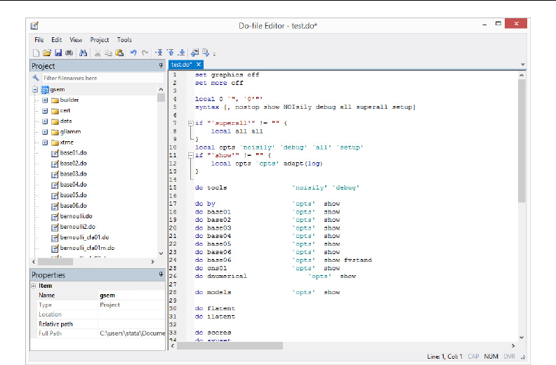
Project Manager — Organize Stata files 403
Figure 1: The Project Manager and Do-file Editor
The left side of the window is the Project Manager. In Windows, the Project Manager pane can
be dragged to other positions in the window. The Project Manager shows the contents of a project
and their properties. The right side of the window is the Do-file Editor. The Do-file Editor is used
to edit Stata text files. See [GSM] 13 Using the Do-file Editor—automating Stata,[GSU] 13 Using
the Do-file Editor—automating Stata, or [GSW] 13 Using the Do-file Editor—automating Stata
for more information about the Do-file Editor.
The Project Manager shows the groups and files in a project in a hierarchical list called a tree
view. Figure 2 shows some of the files and groups in a project we have already created.
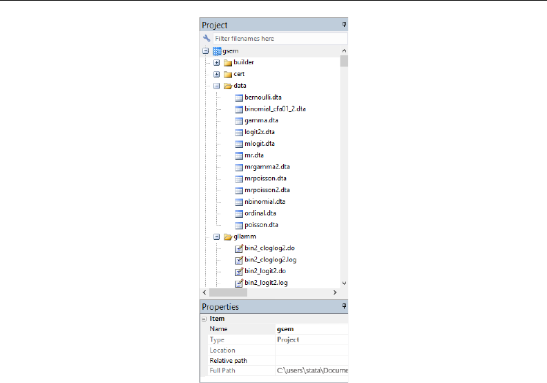
404 Project Manager — Organize Stata files
Figure 2: An open project
The highest level of the hierarchy in the Project Manager is the project. It can contain groups
and files. A group appears in the Project Manager as a folder and is a container for other groups
and files. It is not a reference to a directory on disk. Although you can organize your project in the
Project Manager to reflect the organization of files on disk, moving files into and out of groups does
not affect the content of the directory on disk, and moving files into and out of directories on disk
does not affect the content of the groups in the Project Manager. A file in the Project Manager is a
reference to a file on disk.
Clicking on the disclosure button next to a project or group icon reveals or hides items in the
project. Groups and files are displayed alphabetically in the Project Manager, and groups are always
displayed before files. If a file in a project does not exist on disk, its filename will be displayed in
red.
Below the tree view is the Properties pane, which shows the properties for the current selection.
From the Properties pane, you can rename groups and files, change a file’s relative reference location
on disk to the project, or change a file’s reference to a different file on disk.
On Windows, there is a Search field above the tree view that allows you to filter or search for
files in a project.
On Mac and Unix, the bottom of the Project Manager contains tools for adding or removing groups
and files. On the Mac, there is a single button that displays a menu of possible actions such as adding
and removing groups and files. On Unix, there are separate buttons for adding and removing groups
and files. Next to the buttons is a Search field that allows you to filter or search for files in a project.
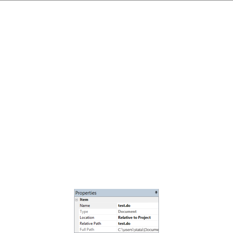
Project Manager — Organize Stata files 405
Editing projects
When starting a new project, we recommend that you create a new directory on disk and store
the project file and the files referenced by the project in the new directory. If you already have a
directory of existing Stata files, save the new project in the directory.
You can add files to a project by dragging the files from disk to the Project Manager or by
right-clicking on an item in the Project Manager and selecting Add Files to "name".... When a
directory on disk is added to a project, its organization on disk at that moment is reflected in the
project. Groups and files can be moved into and out of groups using drag and drop.
To create a new group, select the location in the Project Manager where you want the group added,
right-click, and select Add New Group. You can drag files into the group, and you can drag the
group to a new location in the Project Manager. You can also create a new group from multiple files
by selecting the files, right-clicking on the files, and selecting Add New Group from Selection. A
new group will be created, and the selected files will be moved into the group. You can change the
name of a group by selecting it and entering a new name in the Name edit field.
To remove files from a project, select the files in the Project Manager, right-click on the files, and
select Remove from Project. Removing a file from a project does not delete the file on disk. When
removing a file from a project on the Mac, you can choose to also move the file on disk to the Trash
folder.
Properties
Below the Project Manager’s tree view is the Properties pane. The Properties pane shows the
filename and path for the currently selected item. Figure 3 shows the properties of a do-file that is
currently selected.
Figure 3. Properties of a selected do-file
The Name edit field displays the filename for the currently selected group or file. It can be used to
rename groups and files. If a file is renamed in the project, the file on disk is also renamed. However,
renaming a file on disk does not rename the file in the project and will cause the file to display in
red because it cannot be found.
Below the Name edit field is the Type label. This displays whether the selected item is a project,
group, or document.
Below the Type edit field is the Location pop-up menu. It specifies whether a file’s path is absolute
or relative to the project file. Files that are added to a project have their location set to Relative
to Project by default unless they do not share a common parent directory with the project file. For
example, files that are added from a hard drive different from that of the project file will have their
location set to absolute. You can change a file’s location setting by selecting the appropriate location
setting from the Location pop-up menu.

406 Project Manager — Organize Stata files
The relative path location setting denotes the file’s path in relation to the location of the project
file on disk. If a file is set to use a relative path, the relative path is displayed below the pop-up
menu. Relative paths make projects more portable because you can simply copy a project and all the
files it references to another computer. The file references will stay intact.
The absolute path location setting denotes that the file is at a fixed location on disk. A file in a
project that uses an absolute path will not be affected if its project file is moved. This can be useful
for referencing a Stata dataset that is in a fixed location on disk and is referenced by multiple projects.
Below the Location pop-up menu is the Relink button, which allows you to change a file’s
reference to a different file on disk. It is useful for resolving files that cannot be found. For example,
if you rename a file on disk, the project that references it can no longer find the file. You can use
the Relink button to change a file’s reference to the renamed file.
The full path of a selected file is displayed at the bottom of the Properties pane. The full path is
always displayed as an absolute path regardless of a file’s location setting. On Windows and Mac,
there is a button next to the Full Path text field. Pressing this button will open the file’s parent
directory on the desktop.
Relative versus absolute paths
A relative path denotes a file’s path in relation to the location of the project file on disk. An
absolute path denotes a file’s path at a fixed location on disk. A disadvantage of using absolute paths
is that it makes a project less portable and more difficult to transfer to another computer. In most
cases, you want to use relative paths in your project. There are some situations, however, where you
might want to use absolute paths. For example, you have an extremely large dataset that is used by
different projects, and you do not want to have multiple copies of the dataset taking up disk space.
Another example would be a do-file that is used by different projects that you modify often; keeping
multiple copies of the do-file in sync is difficult.
Relative paths require that projects and their files maintain their relative locations on disk. We
recommend that you create a directory in which to store a project and all of its files and use relative
paths in the project as much as possible. You can then copy the directory to another computer,
including Mac and Unix, and the project can be used as is. By default, the Project Manager uses
relative paths when a file is added to a project. However, it is up to users to use relative paths in
their do-files. The Project Manager is a tool for organizing Stata files, but it cannot ensure that file
references in do-files are maintained, too.
Filtering and searching
The Project Manager can use a filter to display only those files that match a filter text. Click on
the button in the Search field below the Properties pane and select Filter if it is not already selected.
As you enter text, the Project Manager will update and display only those files and groups and parent
groups that contain the text. Figure 4, for example, shows a project filtered to show only do-files
(.do).
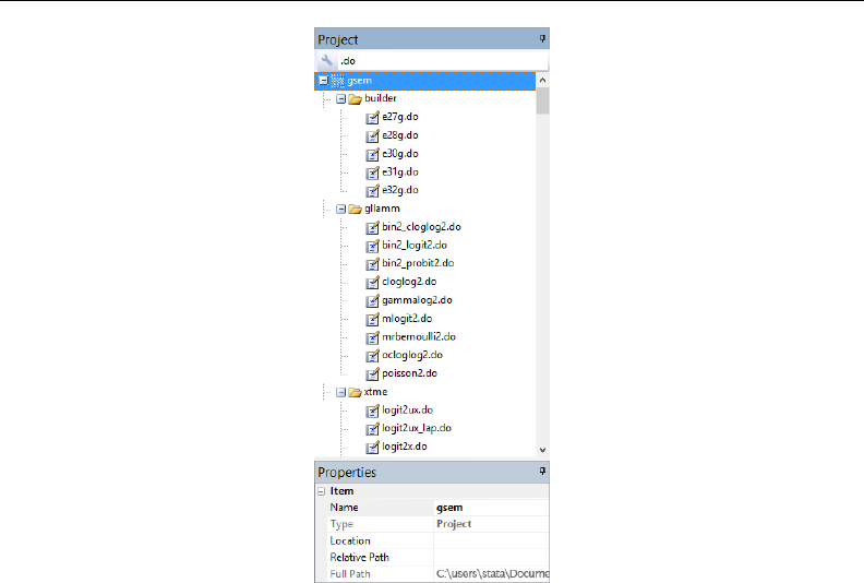
Project Manager — Organize Stata files 407
Figure 4: Filtering
You can move, rename, remove, or add a file or group while a project is filtered. If a file is added
or renamed while a project is filtered, the file will not appear in the filtered list if its filename does
not match the filter text. To stop filtering a project, clear the text in the Search field.
You can also search for a filename in a project. Click on the button in the Search field, and select
Search if it is not already selected. After entering text in the Search field, press the Enter key to
begin the search. If a filename matches the search text, the filename is selected and scrolled into
view. Pressing the Enter key again will search for a matching filename again. If there is no matching
filename beyond the current selection, the search is resumed from the top of the project. Holding
down the Shift key while pressing the Enter key will search in reverse.
Also see
[R]doedit — Edit do-files and other text files

Title
putexcel — Export results to an Excel file
Description Quick start Menu Syntax
Options Remarks and examples Appendix References
Also see
Description
putexcel writes Stata expressions,matrices, images, and returned results to an Excel file. It
may also be used to format cells in an Excel worksheet. This allows you to automate exporting
and formatting of, for example, Stata estimation results. Excel 1997/2003 (.xls) files and Excel
2007/2010 and newer (.xlsx) files are supported.
putexcel set sets the Excel file to create, modify, or replace in subsequent putexcel commands.
You must set the destination file before using any other putexcel commands. putexcel clear
clears the file information set by putexcel set.putexcel describe displays the file information
set by putexcel set.
For the advanced syntax that lets you simultaneously write multiple output types, see [P]putexcel
advanced.
Quick start
Declare the first sheet of myresults.xlsx to be the destination workbook for subsequent putexcel
commands
putexcel set myresults
As above, but use a new sheet named Estimation Results and replace the existing workbook
putexcel set myresults, replace sheet("Estimation Results")
Write the text “Coefficients” to cell B1
putexcel B1 = "Coefficients"
Add variable names and estimated coefficients in the column under “Coefficients” after regress,
and format coefficients with two decimal places
matrix b = e(b)’
putexcel A2 = matrix(b), rownames nformat(number_d2)
Format the header row of the table with a bottom border and bold text
putexcel (A1:B1), bold border(bottom)
Add PNG of a margins plot saved to disk as mymargins.png where the upper-left corner is aligned
with the upper-left corner of cell D2
marginsplot, name(mymargins)
graph export mymargins.png, name(mymargins)
putexcel D2 = picture(mymargins.png)
408

putexcel — Export results to an Excel file 409
Menu
File >Export >Results to Excel spreadsheet (*.xls;*.xlsx)
Syntax
Set workbook for export
putexcel set filename ,set options
Write expression to Excel
putexcel ul cell =exp ,export options format options
Export Stata matrix to Excel
putexcel ul cell = matrix(name),export options format options
Export Stata graph, path diagram, or other picture to Excel
putexcel ul cell = picture(filename)
Export returned results to Excel
putexcel ul cell =returnset ,export options
Write formula to Excel
putexcel ul cell = formula(formula),export options
Format cells
putexcel cellrange,format options
Describe current export settings
putexcel describe
Clear current export settings
putexcel clear
ul cell is a valid Excel upper-left cell specified using standard Excel notation, for example, A1 or D4.
cellrange is ul cell or ul cell:lr cell, where lr cell is a valid Excel lower-right cell, for example,
A1,A1:D1,A1:A4, or A1:D4.
set options Description
sheet(sheetname, replace )specify the worksheet to use; default is the first worksheet
modify modify Excel file
replace overwrite Excel file

410 putexcel — Export results to an Excel file
export options Description
Main
overwritefmt overwrite existing cell formatting when exporting new content
asdate convert Stata date (%td-formatted) exp to an Excel date
asdatetime convert Stata datetime (%tc-formatted) exp to an Excel datetime
asdatenum convert Stata date exp to an Excel date number, preserving the cell’s
format
asdatetimenum convert Stata datetime exp to an Excel datetime number, preserving the
cell’s format
names also write row names and column names for matrix name; may not be
combined with rownames or colnames
rownames also write matrix row names for matrix name; may not be combined
with names or colnames
colnames also write matrix column names for matrix name; may not be combined
with names or rownames
colwise write results in returnset to consecutive columns instead of rows

putexcel — Export results to an Excel file 411
format options Description
Number
nformat(excelnfmt)specify format for numbers
Alignment
left left-align text
hcenter center text horizontally
right right-align text
top vertically align text with the top
vcenter center text vertically
bottom vertically align text with the bottom
txtindent(#)indent text by #spaces; default is 0
txtrotate(#)rotate text by #degrees; default is 0
no txtwrap wrap text within each cell
no shrinkfit shrink text to fit the cell width
merge merge cells in cellrange
unmerge separate merged cells identified by ul cell
Font
font(fontname ,size ,color )specify font, font size, and font color
no italic format text as italic
no bold format text as bold
no underline underline text in the specified cells
no strikeout strikeout text in the specified cells
script(sub |super |none) specify subscript or superscript formatting
Border
border(border ,style ,color )specify horizontal and vertical cell border style
dborder(direction ,style ,color )specify diagonal cell border style
Fill
fpattern(pattern ,fgcolor ,bgcolor )specify fill pattern for cells
Output types
exp writes a valid Stata expression to a cell. See [U] 13 Functions and expressions. Stata dates and
datetimes differ from Excel dates and datetimes. To properly export date and datetime values, use
asdate and asdatetime.
matrix(name)writes the values from a Stata matrix to Excel. Stata determines where to place the
data in Excel by default from the size of the matrix (the number of rows and columns) and the
location you specified in ul cell. By default, ul cell contains the first element of name, and matrix
row names and column names are not written.
picture(filename)writes a portable network graphics (.png), JPEG (.jpg), Windows metafile
(.wmf), device-independent bitmap (.dib), enhanced metafile (.emf), or bitmap (.bmp) file to an
Excel worksheet. The upper-left corner of the image is aligned with the upper-left corner of the
specified ul cell. The image is not resized. If filename contains spaces, it must be enclosed in
double quotes.
returnset is a shortcut name that is used to identify a group of return values. It is intended primarily
for use by programmers and by those who intend to do further processing of their exported results
in Excel. returnset may be any one of the following:

412 putexcel — Export results to an Excel file
returnset
escalars escalarnames
rscalars rscalarnames
emacros emacronames
rmacros rmacronames
ematrices ematrixnames
rmatrices rmatrixnames
e* enames
r* rnames
formula(formula)writes an Excel formula to the cell specified in ul cell.formula may be any valid
Excel formula. Stata does not validate formulas; the text is passed literally to Excel.
Options
Set
sheet(sheetname , replace )saves to the worksheet named sheetname. If there is no worksheet
named sheetname in the workbook, then a new sheet named sheetname is created. If this option
is not specified, the first worksheet of the workbook is used.
replace permits putexcel set to overwrite sheetname if it exists in the specified filename.
modify permits putexcel set to modify an Excel file.
replace permits putexcel set to overwrite an existing Excel workbook. The workbook is overwritten
when the first putexcel command is issued.
Main
overwritefmt causes putexcel to remove any existing cell formatting in the cell or cells to which
it is writing new output. By default, all existing cell formatting is preserved.
asdate tells putexcel that the specified exp is a Stata %td-formatted date that should be converted
to an Excel date with m/d/yyyy Excel date format.
This option has no effect if an exp is not specified as the output type.
asdatetime tells putexcel that the specified exp is a Stata %tc-formatted datetime that should be
converted to an Excel datetime with m/d/yyyy h:mm Excel datetime format.
This option has no effect if an exp is not specified as the output type.
asdatenum tells putexcel that the specified exp is a Stata %td-formatted date that should be converted
to an Excel date number, preserving the cell’s format.
This option has no effect if an exp is not specified as the output type.
asdatetimenum tells putexcel that the specified exp is a Stata %tc-formatted datetime that should
be converted to an Excel datetime number, preserving the cell’s format.
This option has no effect if an exp is not specified as the output type.
names specifies that matrix row names and column names be written into the Excel worksheet along
with the matrix values. If you specify names, then ul cell will be blank, the cell to the right of it
will contain the name of the first column, and the cell below it will contain the name of the first
row. names may not be specified with rownames or colnames.
This option has no effect if matrix() is not specified as the output type.

putexcel — Export results to an Excel file 413
rownames specifies that matrix row names be written into the Excel worksheet along with the matrix
values. If you specify rownames, then ul cell will contain the name of the first row. rownames
may not be specified with names or colnames.
This option has no effect if matrix() is not specified as the output type.
colnames specifies that matrix column names be written into the Excel worksheet along with the
matrix values. If you specify colnames, then ul cell will contain the name of the first column.
colnames may not be specified with names or rownames.
This option has no effect if matrix() is not specified as the output type.
colwise specifies that if a returnset is used, the values written to the Excel worksheet be written in
consecutive columns. By default, the values are written in consecutive rows.
This option has no effect if a returnset is not specified as the output type.
Number
nformat(excelnfmt)changes the numeric format of a cell range. Codes for commonly used formats
are shown in the table of numeric formats in the Appendix. However, any valid Excel format is
permitted. For information about creating your own formats, see the description of nformat() in
Options of [P]putexcel advanced.
Alignment
left sets the specified cells to have contents left-aligned within the cell. left may not be combined
with right or hcenter. Right-alignment is the Excel default for numeric values and need not be
specified when outputting numbers.
hcenter sets the specified cells to have contents horizontally centered within the cell. hcenter may
not be combined with left or right.
right sets the specified cells to have contents right-aligned within the cell. right may not be
combined with left or hcenter. Left-alignment is the Excel default for text and need not be
specified when outputting strings.
top sets the specified cells to have contents vertically aligned with the top of the cell. top may not
be combined with bottom or vcenter.
vcenter sets the specified cells to have contents vertically aligned with the center of the cell. vcenter
may not be combined with top or bottom.
bottom sets the specified cells to have contents vertically aligned with the bottom of the cell. bottom
may not be combined with top or vcenter.
txtindent(#)sets the text indention in each cell in a cell range. #must be an integer between 0
and 15.
txtrotate(#)sets the text rotation in each cell in a cell range. #must be an integer between 0 and
180 or equal to 255. txtrotate(0) is equal to no rotation and is the default. txtrotate(255)
specifies vertical text. Values 1–90 rotate the text counterclockwise 1 to 90 degrees. Values 91–180
rotate the text clockwise 1 to 90 degrees.
txtwrap and notxtwrap specify whether or not the text is to be wrapped in a cell or within each
cell in a range of cells. The default is no wrapping. notxtwrap has an effect only if the cell or
cells were previously formatted to wrap. txtwrap may not be specified with shrinkfit.
shrinkfit and noshrinkfit specify whether or not the text is to be shrunk to fit in the cell width
of a cell or in each cell of a range of cells. The default is no shrinking. noshrinkfit has an

414 putexcel — Export results to an Excel file
effect only if the cell or cells were previously formatted to shrink text to fit. shrinkfit may not
be specified with txtwrap.
merge tells Excel that cells in the specified cell range should be merged. merge may be combined
with left,right,hcenter,top,bottom, and vcenter to format the merged cell. Merging
cells that contain data in each cell will result in the upper-leftmost data being kept.
Once you have merged cells, you can refer to the merged cell by using any single cell from the
specified cellrange. For example, if you specified a cellrange of A1:B2, you could refer to the
merged cell using A1,B1,A2, or B2.
unmerge tells Excel to unmerge previously merged cells. When using unmerge, you only need to
use a single cell from the merged cell in the previously specified cellrange.
Font
font(fontname ,size ,color )sets the font, font size, and font color for each cell in a cell
range. If font() is not specified, the Excel defaults are preserved.
fontname may be any valid Excel font. If fontname includes spaces, then it must be enclosed in
double quotes. What constitutes a valid Excel font is determined by the version of Excel that
is installed on the user’s computer.
size is a numeric value that represents any valid Excel font size. The default is 12.
color may be one of the colors listed in the table of colors in the Appendix or may be a valid
RGB value in the form "### ### ###". If no color is specified, then Excel workbook defaults
are used.
italic and noitalic specify whether to italicize or unitalicize the text in a cell or range of cells.
The default is for text to be unitalicized. noitalic has an effect only if the cell or cells were
previously italicized.
bold and nobold specify whether to bold or unbold the text in a cell or range of cells. The default
is for text to be unbold. nobold has an effect only if the cell or cells were previously formatted
as bold.
underline and nounderline specify whether to underline the text or remove the underline from
the text in a cell or range of cells. The default is for text not to be underlined. nounderline has
an effect only if the cell or cells previously contained underlined text.
strikeout and nostrikeout specify whether to strikeout the text or remove the strikeout from the
text in a cell or range of cells. The default is for text not to have a strikeout mark. nostrikeout
has an effect only if the cell or cells previously had a strikeout mark.
script(sub |super |none) changes the script style of the cell. script(sub) makes all text in a
cell or range of cells a subscript. script(super) makes all text in a cell or range of cells a
superscript. script(none) removes all subscript or superscript formatting from a cell or range of
cells. Specifying script(none) has an effect only if the cell or cells were previously formatted
as subscript or superscript.
Border
border(border ,style ,color )sets the cell border, style, and color for a cell or range of cells.
border may be all,left,right,top, or bottom.
style is a keyword specifying the look of the border. The most common styles are thin,medium,
thick, and double. The default is thin. For a complete list of border styles, see the Appendix.
To remove an existing border, specify none as the style.

putexcel — Export results to an Excel file 415
color may be one of the colors listed in the table of colors in the Appendix or may be a valid
RGB value in the form "### ### ###". If no color is specified, then Excel workbook defaults
are used.
dborder(direction ,style ,color )sets the cell diagonal border direction, style, and color for
a cell or range of cells.
direction may be down,up, or both.down draws a line from the upper-left corner of the cell to
the lower-right corner of the cell or, for a range of cells, from the upper-left corner of ul cell
to the lower-right corner of lr cell.up draws a line from the lower-left corner of the cell to
the upper-right corner of the cell or, for a range of cells, from the lower-left corner of the area
defined by ul cell:lr cell to the upper-right corner.
style is a keyword specifying the look of the border. The most common styles are thin,medium,
thick, and double. The default is thin. For a complete list of border styles, see the Appendix.
To remove an existing border, specify none as the style.
color may be one of the colors listed in the table of colors in the Appendix or may be a valid
RGB value in the form "### ### ###". If no color is specified, then Excel workbook defaults
are used.
Fill
fpattern(pattern ,fgcolor ,bgcolor )sets the fill pattern, foreground color, and background
color for a cell or range of cells.
pattern is a keyword specifying the fill pattern. The most common fill patterns are solid for a
solid color (determined by fgcolor), gray25 for 25% gray scale, gray50 for 50% gray scale,
and gray75 for 75% gray scale. A complete list of fill patterns is shown in the Appendix. To
remove an existing fill pattern from the cell or cells, specify none as the pattern.
fgcolor specifies the foreground color. The default foreground color is black.fgcolor may be any
of the colors listed in the table of colors in the Appendix or may be a valid RGB value in the
form "### ### ###".
bgcolor specifies the background color. bgcolor may be any of the colors listed in the table of
colors in the Appendix or may be a valid RGB value in the form "### ### ###". If no bgcolor
is specified, then Excel workbook defaults are used.

416 putexcel — Export results to an Excel file
Remarks and examples
Remarks are presented under the following headings:
Introduction
Writing expressions and formatting cells
Exporting summary statistics to Excel
Export estimation results
Export graphs and other images
Introduction
The putexcel command is a means of directly controlling the layout of an Excel file. As such,
putexcel is designed to mimic the options and functionality of Excel, and many options of putexcel
are simply pass-through arguments to Excel itself. In what follows, we provide documentation of
how to use the putexcel command. However, for many options, such as the specification of valid
numeric formats, font names, and font sizes, users are encouraged to also consult the help for their
specific version of Excel.
putexcel may be used with Excel 1997/2003 (.xls) and Excel 2007/2010 and newer (.xlsx).
putexcel looks at the file extension .xls or .xlsx to determine which Excel format to write. It is
supported on Windows, Mac, and Linux.
putexcel also has an advanced syntax that allows you to write multiple types of output to different
cells or cell ranges at a time; see [P]putexcel advanced.
Example 1: Setting the workbook and sheet
Before we can write to an Excel workbook using putexcel, we need to tell Stata what the
destination is. We do this using the putexcel set command. For the next several examples, we will
use an Excel file named myresults.xlsx and a sheet named Descriptive.
. putexcel set myresults.xlsx, sheet(Descriptive)
If we had not specified the sheet name, putexcel set would have defaulted to using the first
sheet in the workbook.
Writing expressions and formatting cells
Although there are many uses for putexcel, one of the primary reasons to use the command is
to keep track of the results of analyses in a single location for later use. The next several examples
show how to export results to a single location for easy sharing and to create formatted tables that
can be placed in a paper or poster.
Suppose we are analyzing data about the number of times young adults visited a news website.
These data are contained in website.dta and described in detail in example 1 of [R]ivpoisson.

putexcel — Export results to an Excel file 417
. use http://www.stata-press.com/data/r14/website
(Visits to website)
. describe
Contains data from http://www.stata-press.com/data/r14/website.dta
obs: 500 Visits to website
vars: 6 11 Feb 2014 14:45
size: 13,500
storage display value
variable name type format label variable label
visits byte %8.0g Visits to website
female byte %8.0g Female
ad byte %8.0g Advertisements
time double %10.0g Time on internet (hrs.)
phone double %10.0g Time on phone (hrs.)
frfam double %10.0g Time with friends and out of town
family (hrs.)
Sorted by:
We want to create a formatted table of summary statistics for men and women.
Example 2: Write expression to cell
We start by writing column headers to the first row of our worksheet.
. putexcel A1 = "Variable"
file myresults.xlsx saved
. putexcel B1 = "Men"
file myresults.xlsx saved
. putexcel C1 = "Women"
file myresults.xlsx saved
Each of these commands opens the Excel workbook, writes the text to the specified cell, and then
closes the workbook. We also use expressions to write out specific results (see example 4).
Example 3: Format a range of cells
We may also want to make the column headings bold and add a border underneath. We can format
a range of cells by specifying a cell range and the appropriate formatting options.
. putexcel A1:C1, bold border(bottom)
file myresults.xlsx saved
We also could have specified the bold and border() options each time we exported the column
heading in example 2.
. putexcel A1 = "Variable", bold border(bottom)
file myresults.xlsx saved
. putexcel B1 = "Men", bold border(bottom)
file myresults.xlsx saved
. putexcel C1 = "Women", bold border(bottom)
file myresults.xlsx saved
Whether you apply formatting at the time you write to Excel or for a range will likely depend on
the number of options you have and the number of cells affected by common formatting options.

418 putexcel — Export results to an Excel file
Exporting summary statistics to Excel
We can use putexcel to write summary statistics to an Excel worksheet. The available summary
statistics are determined by returned results. The returned results are documented in the Stored results
section of the command’s manual entry or help. You can also see what is returned by typing return
list or ereturn list.
Example 4: Export selected statistics
To export a specific statistic, we use the expression output type. For example, we might want a
table that has the number of observations for men and women followed by means for each variable,
which we show in example 5.
We can obtain counts many ways in Stata. Here we use the summarize command and restrict
the command to males (female==0). We use visits, but any continuous variable without missing
values would have worked just as well. r(N) stores the number of observations.
. summarize visits if female==0
Variable Obs Mean Std. Dev. Min Max
visits 257 5.105058 3.893185 1 27
. putexcel B2 = ‘r(N)’
file myresults.xlsx saved
A more direct way to obtain the number of observations is with the count command.
. count if female==1
243
. putexcel C2 = ‘r(N)’
file myresults.xlsx saved
Notice that we typed ‘r(N)’ instead of "r(N)". The ‘’ tell Stata to fill in the numeric value
associated with r(N) instead of exporting the text, known as macro substitution; see [P]macro. If
we wanted to treat the contents of r(N), or any other return value, like a string, we could have typed
"‘r(N)’".
Example 5: Export frequency tables
You can use putexcel in Stata to create tables in Excel by using the matrix() output type.
Suppose we want create a table of means for each variable for each value of female. We can use
tabstat with the save option and then check the return values with return list to determine
what values to output.
. tabstat visits ad time phone frfam, by(female) save
Summary statistics: mean
by categories of: female (Female)
female visits ad time phone frfam
0 5.105058 2.175097 3.222412 3.164086 3.65428
1 4.946502 2.098765 3.161276 3.155391 3.676708
Total 5.028 2.138 3.1927 3.15986 3.66518
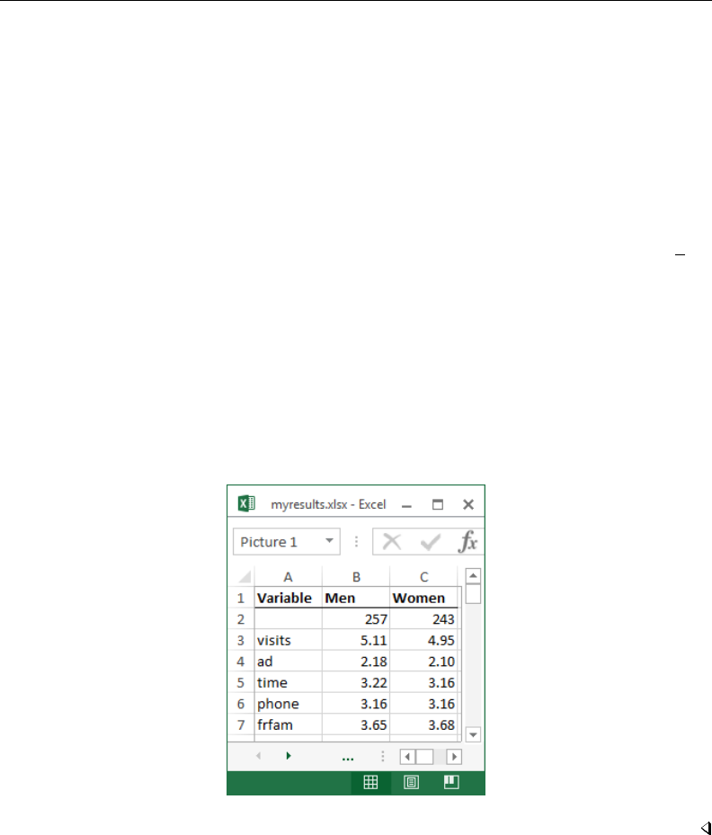
putexcel — Export results to an Excel file 419
. return list
macros:
r(name2) : "1"
r(name1) : "0"
matrices:
r(Stat2) : 1 x 5
r(Stat1) : 1 x 5
r(StatTotal) : 1 x 5
First, we transpose the row vectors r(Stat1) and r(Stat2), which contain the means, so that
the values are written in a column under each heading. We want the variable names to be included, so
for males, which is the first matrix we output, we include the rownames option. Because we want the
values in B3 and the row names of the matrix in A3, we specify A3. We use nformat(number d2)
to format the means with two decimal places. For females, we do not need to specify the names
again, so we just specify the cell where we want the data to be written.
. matrix male = r(Stat1)’
. matrix female = r(Stat2)’
. putexcel A3 = matrix(male), rownames nformat(number_d2)
file myresults.xlsx saved
. putexcel C3 = matrix(female), nformat(number_d2)
file myresults.xlsx saved
The above commands give a final table of frequencies and means that looks like this:
Export estimation results
A similar approach to that used in example 5 can be used to export estimation results. Suppose
we want to fit a linear regression model of visits as a function of ad,female, and time using
regress and we want to export formatted results.

420 putexcel — Export results to an Excel file
. regress visits ad female time
Source SS df MS Number of obs = 500
F(3, 496) = 346.75
Model 5710.6792 3 1903.55973 Prob > F = 0.0000
Residual 2722.9288 496 5.4897758 R-squared = 0.6771
Adj R-squared = 0.6752
Total 8433.608 499 16.901018 Root MSE = 2.343
visits Coef. Std. Err. t P>|t| [95% Conf. Interval]
ad .7996179 .0516591 15.48 0.000 .6981203 .9011156
female -.0467997 .2096816 -0.22 0.823 -.4587734 .3651739
time .82962 .0436601 19.00 0.000 .7438385 .9154014
_cons .6924339 .2007914 3.45 0.001 .2979273 1.086941
Example 6: Export point estimates and sample size
We start by using putexcel set again to create a new worksheet for our regression results.
. putexcel set myresults.xlsx, sheet(Estimation)
We want to give our coefficients the title “Coef.” in the table we create, so we use an expression to
write this to cell B1. We create a new matrix for our coefficients as the transpose of the values of
e-class matrix e(b). We use column A row 2 as the starting location for the matrix row labels, and
we use column B row 2 as the starting location for the coefficients; to do this, we only need to specify
the upper-left cell (A2) and the rownames option. To make our table more readable, we format the
coefficient estimates with two decimal places by using nformat() and add a bottom border under
the estimates.
. putexcel B1 = "Coef."
file myresults.xlsx saved
. matrix b = e(b)’
. putexcel A2 = matrix(b), rownames nformat(number_d2)
file myresults.xlsx saved
. putexcel A5:B5, border(bottom)
file myresults.xlsx saved
We then add a right-aligned and italicized “N=” in column A row 6 and the sample size from
e-class scalar e(N) in column B row 6. We use a medium border under this row instead of the default
thin border to indicate that the table is complete.
. putexcel A6 = "N=", italic right border(bottom, medium)
file myresults.xlsx saved
. putexcel B6 = matrix(e(N)), nformat(number_sep) border(bottom, medium)
file myresults.xlsx saved
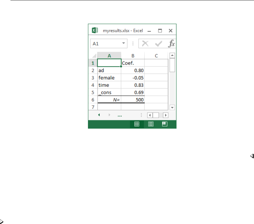
putexcel — Export results to an Excel file 421
The above commands create a table that looks like this:
If you are going to export more complex tables or many objects, you should use the advanced
syntax of putexcel; see [P]putexcel advanced.
Export graphs and other images
You can export PNG,JPEG, and other image formats to Excel with putexcel. To export a Stata
graph, you must first use graph export to convert the Stata graph to one of the supported image
formats.
Example 7: Export Stata graph
We may want to add a histogram about the number of advertisements viewed to our set of
descriptive results. We can use the histogram command and then graph export to create a PNG
file of our histogram.
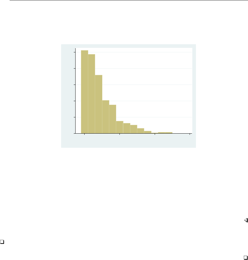
422 putexcel — Export results to an Excel file
. histogram ad, discrete
(start=0, width=1)
. graph export ads.png
(file ads.png written in PNG format)
0 .05 .1 .15 .2 .25
Density
0 5 10 15
Advertisements
Next, we use putexcel set to switch back to the Excel sheet named Descriptive, and then
we output the graph to Excel with the picture() output type.
. putexcel set myresults.xlsx, sheet(Descriptive)
. putexcel E2 = picture(ads.png)
file myresults.xlsx saved
This adds the graph with the upper-left corner of the graph aligned in the upper-left corner of cell E2.
Graphs are not resized by putexcel, but you can change the size with the graph export command;
see [G-2]graph export.
Technical note
See the technical notes Excel data size limits and Dates and times in [D]import excel.

putexcel — Export results to an Excel file 423
Appendix
Codes for numeric formats
Code Example
number 1000
number d2 1000.00
number sep 100,000
number sep d2 100,000.00
number sep negbra (1,000)
number sep negbrared (1,000)
number d2 sep negbra (1,000.00)
number d2 sep negbrared (1,000.00)
currency negbra ($4000)
currency negbrared ($4000)
currency d2 negbra ($4000.00)
currency d2 negbrared ($4000.00)
account 5,000
accountcur $ 5,000
account d2 5,000.00
account d2 cur $ 5,000.00
percent 75%
percent d2 75.00%
scientific d2 10.00E+1
fraction onedig 10 1/2
fraction twodig 10 23/95
date 3/18/2007
date d mon yy 18-Mar-07
date d mon 18-Mar
date mon yy Mar-07
time hmm AM 8:30 AM
time HMMSS AM 8:30:00 AM
time HMM 8:30
time HMMSS 8:30:00
time MMSS 30:55
time H0MMSS 20:30:55
time MMSS0 30:55.0
date time 3/18/2007 8:30
text this is text

424 putexcel — Export results to an Excel file
Colors
color
aliceblue deeppink
antiquewhite deepskyblue
aqua dimgray
aquamarine dodgerblue
azure firebrick
beige floralwhite
bisque forestgreen
black fuchsia
blanchedalmond gainsboro
blue ghostwhite
blueviolet gold
brown goldenrod
burlywood gray
cadetblue green
chartreuse greenyellow
chocolate honeydew
coral hotpink
cornflowerblue indianred
cornsilk indigo
crimson ivory
cyan khaki
darkblue lavender
darkcyan lavenderblush
darkgoldenrod lawngreen
darkgray lemonchiffon
darkgreen lightblue
darkkhaki lightcoral
darkmagenta lightcyan
darkolivegreen lightgoldenrodyellow
darkorange lightgray
darkorchid lightgreen
darkred lightpink
darksalmon lightsalmon
darkseagreen lightseagreen
darkslateblue lightskyblue
darkslategray lightslategray
darkturquoise lightsteelblue
darkviolet lightyellow

putexcel — Export results to an Excel file 425
color,continued
lime peru
limegreen pink
linen plum
magenta powerblue
maroon purple
mediumaquamarine red
mediumblue rosybrown
mediumorchid royalblue
mediumpurple saddlebrown
mediumseagreen salmon
mediumslateblue sandybrown
mediumspringgreen seagreen
mediumturquoise seashell
mediumvioletred sienna
midnightblue silver
mintcream skyblue
mistyrose slateblue
moccasin snow
navajowhite springgreen
navy steelblue
oldlace tan
olive teal
olivedrab thistle
orange tomato
orangered turquoise
orchid violet
palegoldenrod wheat
palegreen white
paleturquoise whitesmoke
palevioletred yellow
papayawhip yellowgreen
peachpuff

426 putexcel — Export results to an Excel file
Border styles
style
none
thin
medium
dashed
dotted
thick
double
hair
medium dashed
dash dot
medium dash dot
dash dot dot
medium dash dot dot
slant dash dot
Background patterns
pattern
none
solid
gray50
gray75
gray25
horstripe
verstripe
diagstripe
revdiagstripe
diagcrosshatch
thinhorstripe
thinverstripe
thindiagstripe
thinrevdiagstripe
thinhorcrosshatch
thindiagcrosshatch
thickdiagcrosshatch
gray12p5
gray6p25

putexcel — Export results to an Excel file 427
References
Crow, K. 2013. Export tables to Excel. The Stata Blog: Not Elsewhere Classified.
http://blog.stata.com/2013/09/25/export-tables-to-excel/.
Gallup, J. L. 2012. A new system for formatting estimation tables.Stata Journal 12: 3–28.
Quint´
o, L. 2012. HTML output in Stata.Stata Journal 12: 702–717.
Also see
[P]putexcel advanced — Export results to an Excel file using advanced syntax
[P]postfile — Post results in Stata dataset
[P]return — Return stored results
[D]export — Overview of exporting data from Stata
[D]import — Overview of importing data into Stata
[M-5]docx*( ) — Generate Office Open XML (.docx) file
[M-5]xl( ) — Excel file I/O class

Title
putexcel advanced — Export results to an Excel file using advanced syntax
Description Quick start Menu Syntax
Options Remarks and examples References Also see
Description
putexcel with the advanced syntax may be used to simultaneously write Stata expressions,
matrices, images, and stored results to an Excel file. It may also be used to format existing contents
of cells in a worksheet. This syntax is intended for use by programmers of commands that call
putexcel in the background and by other advanced users. Excel 1997/2003 (.xls) files and Excel
2007/2010 and newer (.xlsx) files are supported. A simplified version of the syntax is documented
in [P]putexcel.
putexcel set sets the Excel file to create, modify, or replace in subsequent putexcel commands.
You must set the destination file before using any other putexcel commands. putexcel clear
clears the file information set by putexcel set.putexcel describe displays the file information
set by putexcel set.
Quick start
Declare the first sheet of myresults.xlsx to be the destination workbook for subsequent putexcel
commands
putexcel set myresults
As above, but use a sheet named Estimation Results and replace that sheet if it exists
putexcel set myresults, sheet("Estimation Results", replace)
Write estimation results in e(b) to column B, starting in row 2, with the results formatted to have
two decimal places, matrix row names in column A, and the title “Coefs.” in cell B1
matrix b=e(b)’
putexcel B1="Coefs." A2=matrix(b), rownames nformat(number_d2)
Add a thin border under cells A1 to B1 and italicize the text
putexcel (A1:B1), border(bottom) italic
Write “Some text that is too long to fit” to cell D1 and set the text to wrap within the cell
putexcel D1="Some text that is too long to fit", txtwrap
Merge D1 with D2, E1, and E2, and horizontally and vertically center
putexcel (D1:E2), merge hcenter vcenter
Menu
File >Export >Results to Excel spreadsheet (*.xls;*.xlsx)
428

putexcel advanced — Export results to an Excel file using advanced syntax 429
Syntax
Set workbook for export
putexcel set filename ,set options
Specify formatting and output
putexcel spec1spec2. . . ,export options format options
Describe current export settings
putexcel describe
Clear current export settings
putexcel clear
spec may be ul cell or cellrange of the form ul cell:lr cell if no output is to be written or may be
one of the following output types:
ul cell =exp
ul cell:lr cell =exp
ul cell = matrix(name)
ul cell = picture(filename)
ul cell = formula(formula)
ul cell =returnset
ul cell is a valid Excel upper-left cell specified using standard Excel notation, and lr cell is a valid
Excel lower-right cell. If you specify ul cell as the output location multiple times, the rightmost
specification is the one written to the Excel file.
set options Description
sheet(sheetname, replace )specify the worksheet to use; default is the first worksheet
modify modify Excel file
replace overwrite Excel file

430 putexcel advanced — Export results to an Excel file using advanced syntax
export options Description
Main
overwritefmt overwrite existing cell formatting when exporting new content
asdate convert Stata date (%td-formatted) exp to an Excel date
asdatetime convert Stata datetime (%tc-formatted) exp to an Excel datetime
asdatenum convert Stata date exp to an Excel date number, preserving the cell’s
format
asdatetimenum convert Stata datetime exp to an Excel datetime number, preserving the
cell’s format
names also write row names and column names for matrix name; may not be
combined with rownames or colnames
rownames also write matrix row names for matrix name; may not be combined
with names or colnames
colnames also write matrix column names for matrix name; may not be combined
with names or rownames
colwise write results in returnset to consecutive columns instead of rows

putexcel advanced — Export results to an Excel file using advanced syntax 431
format options Description
Number
nformat(excelnfmt)specify format for numbers
Alignment
left left-align text
hcenter center text horizontally
right right-align text
top vertically align text with the top
vcenter center text vertically
bottom vertically align text with the bottom
txtindent(#)indent text by #spaces; default is 0
txtrotate(#)rotate text by #degrees; default is 0
no txtwrap wrap text within each cell
no shrinkfit shrink text to fit the cell width
merge merge cells in cellrange
unmerge separate merged cells identified by ul cell
Font
font(fontname ,size ,color )specify font, font size, and font color
no italic format text as italic
no bold format text as bold
no underline underline text in the specified cells
no strikeout strikeout text in the specified cells
script(sub |super |none) specify subscript or superscript formatting
Border
border(border ,style ,color )specify horizontal and vertical cell border style
dborder(direction ,style ,color )specify diagonal cell border style
Fill
fpattern(pattern ,fgcolor ,bgcolor )specify fill pattern for cells
Output types
exp writes a valid Stata expression to a cell. See [U] 13 Functions and expressions. Stata dates and
datetimes differ from Excel dates and datetimes. To properly export date and datetime values, use
asdate and asdatetime.
matrix(name)writes the values from a Stata matrix to Excel. Stata determines where to place the
data in Excel by default from the size of the matrix (the number of rows and columns) and the
location you specified in ul cell. By default, ul cell contains the first element of name, and matrix
row names and column names are not written.
picture(filename)writes a portable network graphics (.png), JPEG (.jpg), Windows metafile
(.wmf), device-independent bitmap (.dib), enhanced metafile (.emf), or bitmap (.bmp) file to an
Excel worksheet. The upper-left corner of the image is aligned with the upper-left corner of the
specified ul cell. The image is not resized. If filename contains spaces, it must be enclosed in
double quotes.
returnset is a shortcut name that is used to identify a group of return values. returnset may be any
one of the following:

432 putexcel advanced — Export results to an Excel file using advanced syntax
returnset
escalars escalarnames
rscalars rscalarnames
emacros emacronames
rmacros rmacronames
ematrices ematrixnames
rmatrices rmatrixnames
e* enames
r* rnames
formula(formula)writes an Excel formula to the cell specified in ul cell.formula may be any valid
Excel formula. Stata does not validate formulas; the text is passed literally to Excel.
Options
Set
sheet(sheetname , replace )saves to the worksheet named sheetname. If there is no worksheet
named sheetname in the workbook, then a new sheet named sheetname is created. If this option
is not specified, the first worksheet of the workbook is used.
replace permits putexcel set to overwrite sheetname if it exists in the specified filename.
modify permits putexcel set to modify an Excel file.
replace permits putexcel set to overwrite an existing Excel workbook. The workbook is overwritten
when the first putexcel command is issued.
Main
overwritefmt causes putexcel to remove any existing cell formatting in the cell or cells to which
it is writing new output. By default, all existing cell formatting is preserved.
asdate tells putexcel that the specified exp is a Stata %td-formatted date that should be converted
to an Excel date with m/d/yyyy Excel date format.
This option has no effect if an exp is not specified as one of the output types.
asdatetime tells putexcel that the specified exp is a Stata %tc-formatted datetime that should be
converted to an Excel datetime with m/d/yyyy h:mm Excel datetime format.
This option has no effect if an exp is not specified as one of the output types.
asdatenum tells putexcel that the specified exp is a Stata %td-formatted date that should be converted
to an Excel date number, preserving the cell’s format.
This option has no effect if an exp is not specified as one of the output types.
asdatetimenum tells putexcel that the specified exp is a Stata %tc-formatted datetime that should
be converted to an Excel datetime number, preserving the cell’s format.
This option has no effect if an exp is not specified as one of the output types.
names specifies that matrix row names and column names be written into the Excel worksheet along
with the matrix values. If you specify names, then ul cell will be blank, the cell to the right of it
will contain the name of the first column, and the cell below it will contain the name of the first
row. names may not be specified with rownames or colnames.
This option has no effect if matrix() is not specified as one of the output types.

putexcel advanced — Export results to an Excel file using advanced syntax 433
rownames specifies that matrix row names be written into the Excel worksheet along with the matrix
values. If you specify rownames, then ul cell will contain the name of the first row. rownames
may not be specified with names or colnames.
This option has no effect if matrix() is not specified as one of the output types.
colnames specifies that matrix column names be written into the Excel worksheet along with the
matrix values. If you specify colnames, then ul cell will contain the name of the first column.
colnames may not be specified with names or rownames.
This option has no effect if matrix() is not specified as one of the output types.
colwise specifies that if a returnset is used, the values written to the Excel worksheet be written in
consecutive columns. By default, the values are written in consecutive rows.
This option has no effect if a returnset is not specified as one of the output types.
Number
nformat(excelnfmt)changes the numeric format of a cell range. Any valid Excel format is permitted.
Formats are formed from combinations of the following symbols.
Cell Fmt Cell
Symbol Description value code displays
0Digit placeholder (add zeros) 8.9 #.00 8.90
#Digit placeholder (no zeros) 8.9 #.## 8.9
?Digit placeholder (add space) 8.9 0.0? 8.9
.Decimal point
%Percentage .1 %10%
,Thousands separator 10000 #,### 10,000
E- E+ e- e+ Scientific format 12200000 0.00E+00 1.22E+07
$-+/():space Display the symbol 12 (000) (012)
\Escape character 3 0\! 3!
*Repeat character 3 3* 3xxxxx
(fill in cell width)
Skip width of next character −1.2 0.0 1.2
"text" Display text in quotes 1.23 0.00 "a" 1.23 a
@Text placeholder b "a"@"c" abc
Formats that contain spaces must be enclosed in double quotes. A list of codes for common
numeric formats is also shown in the Appendix of [P]putexcel.
Alignment
left sets the specified cells to have contents left-aligned within the cell. left may not be combined
with right or hcenter. Right-alignment is the Excel default for numeric values and need not be
specified when outputting numbers.
hcenter sets the specified cells to have contents horizontally centered within the cell. hcenter may
not be combined with left or right.
right sets the specified cells to have contents right-aligned within the cell. right may not be
combined with left or hcenter. Left-alignment is the Excel default for text and need not be
specified when outputting strings.

434 putexcel advanced — Export results to an Excel file using advanced syntax
top sets the specified cells to have contents vertically aligned with the top of the cell. top may not
be combined with bottom or vcenter.
vcenter sets the specified cells to have contents vertically aligned with the center of the cell. vcenter
may not be combined with top or bottom.
bottom sets the specified cells to have contents vertically aligned with the bottom of the cell. bottom
may not be combined with top or vcenter.
txtindent(#)sets the text indention in each cell in a cell range. #must be an integer between 0
and 15.
txtrotate(#)sets the text rotation in each cell in a cell range. #must be an integer between 0 and
180 or equal to 255. txtrotate(0) is equal to no rotation and is the default. txtrotate(255)
specifies vertical text. Values 1–90 rotate the text counterclockwise 1 to 90 degrees. Values 91–180
rotate the text clockwise 1 to 90 degrees.
txtwrap and notxtwrap specify whether or not the text is to be wrapped in a cell or within each
cell in a range of cells. The default is no wrapping. notxtwrap has an effect only if the cell or
cells were previously formatted to wrap. txtwrap may not be specified with shrinkfit.
shrinkfit and noshrinkfit specify whether or not the text is to be shrunk to fit in the cell width
of a cell or in each cell of a range of cells. The default is no shrinking. noshrinkfit has an
effect only if the cell or cells were previously formatted to shrink text to fit. shrinkfit may not
be specified with txtwrap.
merge tells Excel that cells in the specified cell range should be merged. merge may be combined
with left,right,hcenter,top,bottom, and vcenter to format the merged cell. Merging
cells that contain data in each cell will result in the upper-leftmost data being kept.
Once you have merged cells, you can refer to the merged cell by using any single cell from the
specified cellrange. For example, if you specified a cellrange of A1:B2, you could refer to the
merged cell using A1,B1,A2, or B2.
unmerge tells Excel to unmerge previously merged cells. When using unmerge, you only need to
use a single cell from the merged cell in the previously specified cellrange.
Font
font(fontname ,size ,color )sets the font, font size, and font color for each cell in a cell
range. If font() is not specified, the Excel defaults are preserved.
fontname may be any valid Excel font. If fontname includes spaces, then it must be enclosed in
double quotes. What constitutes a valid Excel font is determined by the version of Excel that
is installed on the user’s computer.
size is a numeric value that represents any valid Excel font size. The default is 12.
color may be a valid RGB value in the form "### ### ###"or may be one of the colors listed
in the table of colors in the Appendix in [P]putexcel. If no color is specified, then Excel
workbook defaults are used.
italic and noitalic specify whether to italicize or unitalicize the text in a cell or range of cells.
The default is for text to be unitalicized. noitalic has an effect only if the cell or cells were
previously italicized.
bold and nobold specify whether to bold or unbold the text in a cell or range of cells. The default
is for text to be unbold. nobold has an effect only if the cell or cells were previously formatted
as bold.

putexcel advanced — Export results to an Excel file using advanced syntax 435
underline and nounderline specify whether to underline the text or remove the underline from
the text in a cell or range of cells. The default is for text not to be underlined. nounderline has
an effect only if the cell or cells previously contained underlined text.
strikeout and nostrikeout specify whether to strikeout the text or remove the strikeout from the
text in a cell or range of cells. The default is for text not to have a strikeout mark. nostrikeout
has an effect only if the cell or cells previously had a strikeout mark.
script(sub |super |none) changes the script style of the cell. script(sub) makes all text in a
cell or range of cells a subscript. script(super) makes all text in a cell or range of cells a
superscript. script(none) removes all subscript or superscript formatting from a cell or range of
cells. Specifying script(none) has an effect only if the cell or cells were previously formatted
as subscript or superscript.
Border
border(border ,style ,color )sets the cell border, style, and color for a cell or range of cells.
border may be all,left,right,top, or bottom.
style is a keyword specifying the look of the border. The most common styles are thin,medium,
thick, and double. The default is thin. For a complete list of border styles, see the Appendix
in [P]putexcel. To remove an existing border, specify none as the style.
color may be a valid RGB value in the form "### ### ###"or may be one of the colors listed
in the table of colors in the Appendix in [P]putexcel. If no color is specified, then Excel
workbook defaults are used.
dborder(direction ,style ,color )sets the cell diagonal border direction, style, and color for
a cell or range of cells.
direction may be down,up, or both.down draws a line from the upper-left corner of the cell to
the lower-right corner of the cell or, for a range of cells, from the upper-left corner of ul cell
to the lower-right corner of lr cell.up draws a line from the lower-left corner of the cell to
the upper-right corner of the cell or, for a range of cells, from the lower-left corner of the area
defined by ul cell:lr cell to the upper-right corner.
style is a keyword specifying the look of the border. The most common styles are thin,medium,
thick, and double. The default is thin. For a complete list of border styles, see the Appendix
in [P]putexcel. To remove an existing border, specify none as the style.
color may be a valid RGB value in the form "### ### ###"or may be one of the colors listed
in the table of colors in the Appendix in [P]putexcel. If no color is specified, then Excel
workbook defaults are used.
Fill
fpattern(pattern ,fgcolor ,bgcolor )sets the fill pattern, foreground color, and background
color for a cell or range of cells.
pattern is a keyword specifying the fill pattern. The most common fill patterns are solid for a
solid color (determined by fgcolor), gray25 for 25% gray scale, gray50 for 50% gray scale,
and gray75 for 75% gray scale. A complete list of fill patterns is shown in the Appendix
of [P]putexcel. To remove an existing fill pattern from the cell or cells, specify none as the
pattern.
fgcolor specifies the foreground color. The default foreground color is black.fgcolor may be a
valid RGB value in the form "### ### ###"or may be any of the colors listed in the table of
colors in the Appendix in [P]putexcel.

436 putexcel advanced — Export results to an Excel file using advanced syntax
bgcolor specifies the background color. bgcolor may be a valid RGB value in the form "### ###
###"or may be any of the colors listed in the table of colors in the Appendix in [P]putexcel.
If no bgcolor is specified, then Excel workbook defaults are used.
Remarks and examples
If you have not already read Remarks and examples in [P]putexcel, please do so now. The
examples here build on the examples shown there.
Remarks are presented under the following headings:
Writing expressions and formatting cells
Using formulas
Exporting estimation results
Writing expressions and formatting cells
Before we can write to an Excel workbook using putexcel, we need to tell Stata what the
destination is. We do this using the putexcel set command. For the next several examples, we will
use an Excel file named myresults2.xlsx. We will begin with a sheet named Descriptive.
. putexcel set myresults2.xlsx, sheet(Descriptive)
If we had not specified the sheet name, putexcel would have defaulted to using the first sheet
in the workbook.
Example 1: Write multiple expressions and format cells simultaneously
Suppose we want to write the same headers and format them as shown in example 2 and example 3
of [P]putexcel. Using the advanced syntax of putexcel, we can do this with a single putexcel
command.
. putexcel A1="Variable" B1="Men" C1="Women", bold border(bottom)
file myresults2.xlsx saved
Rather than beginning with the table headers, we could improve record keeping by including the
date we generated the results. To do this, we can use the system parameter, or c-class return value,
c(current date), which will add a string date in the format dd Mon yyyy; see [P]creturn. We also
merge cells A1 and B1 for aesthetic reasons. Notice that we type "‘c(current date)’" instead
of "c(current date)". The ‘’ indicate macro substitution; see [P]macro. We specify replace
as a suboption to sheet() in a new putexcel set command to overwrite our previous output.
. putexcel set myresults2.xlsx, sheet(Descriptive, replace)
. putexcel A1 = "Results last updated" D1 = "‘c(current_date)’"
file myresults2.xlsx saved
. putexcel (A1:C1), merge
file myresults2.xlsx saved
. putexcel A2="Variable" B2="Men" C2="Women", bold border(bottom)
file myresults2.xlsx saved
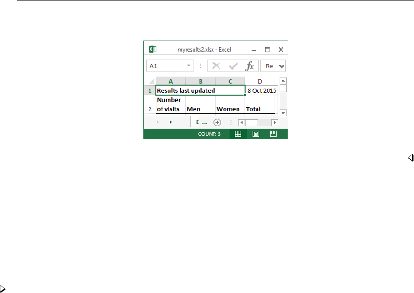
putexcel advanced — Export results to an Excel file using advanced syntax 437
The above commands give an Excel file with a header row that looks like this:
Using formulas
Writing Excel formulas is useful when you want to perform calculations using the output of Stata
commands. Formulas are passed verbatim to Excel, so you must use the correct Excel function (not
Stata function) for what you want to accomplish. You may find it helpful to experiment in Excel first
and then copy the formula over to your do-file to keep a record of your work and in case you need
to run your analysis again later.
Example 2: Adding a total row and total column
In example 4 of [P]putexcel, we obtained the number of females and number of males in the
website dataset and wrote these out to Excel. Suppose instead that we want the number of males
and females at each number of visits and the total number of visits.
We can change the heading for the first column from “Variable” to “Number of visits” and add a
column for “Total”. We specify the txtwrap option with our putexcel command so that the long
text “Number of visits” wraps within cell A2.
We use the matcell() option with tabulate to save the cell frequencies to a matrix and the
matrow() option to save the row values from the table.

438 putexcel advanced — Export results to an Excel file using advanced syntax
. use http://www.stata-press.com/data/r14/website
(Visits to website)
. putexcel A2="Number of visits" D2="Total", txtwrap bold border(bottom)
file myresults2.xlsx saved
. tabulate visits female, matrow(nvisits) matcell(freq)
Visits to Female
website 0 1 Total
1 18 17 35
2 58 42 100
3 32 46 78
4 35 25 60
5 24 40 64
6 21 17 38
7 21 21 42
8 12 7 19
9 8 10 18
10 8 5 13
11 3 5 8
12 4 1 5
13 2 2 4
14 4 0 4
15 1 1 2
16 1 1 2
18 1 0 1
20 2 1 3
22 1 0 1
23 0 1 1
27 1 0 1
51 0 1 1
Total 257 243 500
. putexcel A3=matrix(nvisits) B3=matrix(freq)
file myresults2.xlsx saved
Totals, however, are not saved. By using formulas in Excel, we can add the row and column totals.
Our results will begin on row 3, so we will want to begin calculating row totals here. For example,
in Excel the row total for males (column B) and females (column C) in row 3 is D3=B3+C3. The
fastest way to write this formula multiple times for each row is to use forvalues; see [P]forvalues.
. forvalues i=3/24 {
2. putexcel D‘i’=formula(B‘i’+C‘i’)
3. }
file myresults2.xlsx saved
(output omitted )
We also want column totals. For this, it is easier to use Excel’s SUM() function. We supply this
as the formula() output type and add a border above the total row to set it apart from the rest of
the table.
. putexcel A25="Total" B25=formula(SUM(B3:B24)) C25=formula(SUM(C3:C24))
> D25=formula(SUM(D3:D24)), bold border(top)
file myresults2.xlsx saved

putexcel advanced — Export results to an Excel file using advanced syntax 439
Exporting estimation results
We start by using putexcel set again to create a new worksheet for our regression results.
. putexcel set myresults2.xlsx, sheet(Estimation)
Example 3: Export point estimates and formatted confidence intervals
We continue from example 6 of [P]putexcel, where we gave the coefficients the title “Coef.”.
Here we add a column named “C.I.” for the confidence interval, which we center in cells C1 and D1.
. putexcel B1="Coef." C1="C.I."
file myresults2.xlsx saved
. putexcel (C1:D1), merge hcenter
file myresults2.xlsx saved
We fit the same model that we did in example 6 of [P]putexcel. We copy the r-class return
r(table), which contains the values that were returned by the command in the estimation results
table, into a new matrix named table.
. quietly regress visits ad female time
. matrix table = r(table)
. matrix list table
table[9,4]
ad female time _cons
b .79961794 -.04679974 .82961995 .69243389
se .05165911 .2096816 .04366007 .20079144
t 15.47874 -.22319432 19.001801 3.448523
pvalue 2.235e-44 .82347616 6.794e-61 .00061166
ll .69812028 -.45877341 .74383847 .29792725
ul .90111561 .36517393 .91540143 1.0869405
df 496 496 496 496
crit 1.9647583 1.9647583 1.9647583 1.9647583
eform 0 0 0 0
We then select row 1 for the coefficients (b), row 5 for the lower limit of the confidence interval
(ll), and row 6 for the upper limit of the confidence interval (ul) into separate vectors. We take the
transpose to ensure that our results for each variable are in a row rather than in a column when we
write them out. We specify nformat(number d2) for the coefficients, but we will specify a custom
format for the confidence interval. We also add the rownames option so that the variable names are
written out along with the coefficient estimates.
. matrix b = table[1, 1...]’
. matrix ll = table[5, 1...]’
. matrix ul = table[6, 1...]’
. putexcel A2=matrix(b), rownames nformat(number_d2)
file myresults2.xlsx saved
We want our confidence interval to be displayed as (0.74 to 0.92), taking time, for example. That
is, the numbers should have a 0 before the decimal and be rounded to two decimal places. The lower
and upper limits should be separated by the word “to”, and the confidence interval should be enclosed
in parentheses.
We specify our format in two steps. For the lower limit, we ensure that the negative sign will
display inside the parentheses by specifying separate formats for positive and negative numbers.
The code for positive numbers is specified before the semicolon. The code for negative numbers is
specified after the semicolon. We add the word “to” so that it is printed between the lower and upper
limit values. For the upper limit, the negative sign will display in front of the number by default, so
we only have to specify one format.
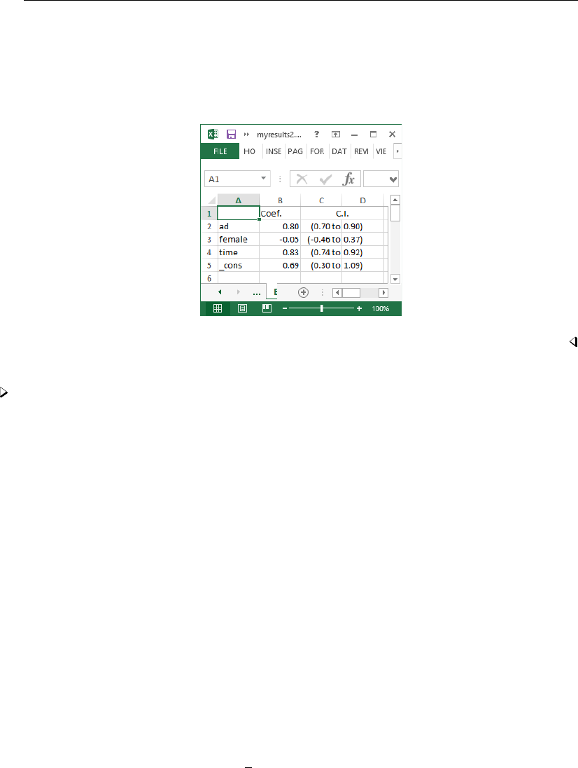
440 putexcel advanced — Export results to an Excel file using advanced syntax
. putexcel C2=matrix(ll), nformat("(0.00 to;(-0.00 to") right
file myresults2.xlsx saved
. putexcel D2=matrix(ul), nformat("0.00)") left
file myresults2.xlsx saved
The above commands give a table that looks like this:
Example 4: Export SEM estimates and path diagram
Continuing example 3, suppose we also fit a corresponding linear regression model using sem and
want to export the coefficient estimates, confidence intervals, and the path diagram. We use the same
general approach as in example 3 but with some modification. First, we specify the range of columns
from table to be 1 through 4 when we create our b,ll, and ul vectors to exclude the variance.
. quietly sem (visits <- ad female time)
. matrix table = r(table)
. matrix list table
table[9,5]
visits: visits: visits: visits: var(e.vis~):
ad female time _cons _cons
b .79961794 -.04679974 .82961995 .69243389 5.4458576
se .05145206 .20884119 .04348508 .19998666 .34442628
z 15.541029 -.22409249 19.078268 3.4624004 .b
pvalue 1.830e-54 .82268533 3.827e-81 .00053538 .b
ll .69877376 -.45612096 .74439077 .30046724 4.810958
ul .90046212 .36252147 .91484914 1.0844005 6.1645445
df.....
crit 1.959964 1.959964 1.959964 1.959964 1.959964
eform 0 0 0 0 0
. matrix b = table[1, 1..4]’
. matrix ll = table[5, 1..4]’
. matrix ul = table[6, 1..4]’
If we wanted that term as well, we could select it separately. Because we do not need to specify
row names again, we also specify the ul cell for bin reference to its values, not the labels this time.
We use the same numeric format for ll and ul.
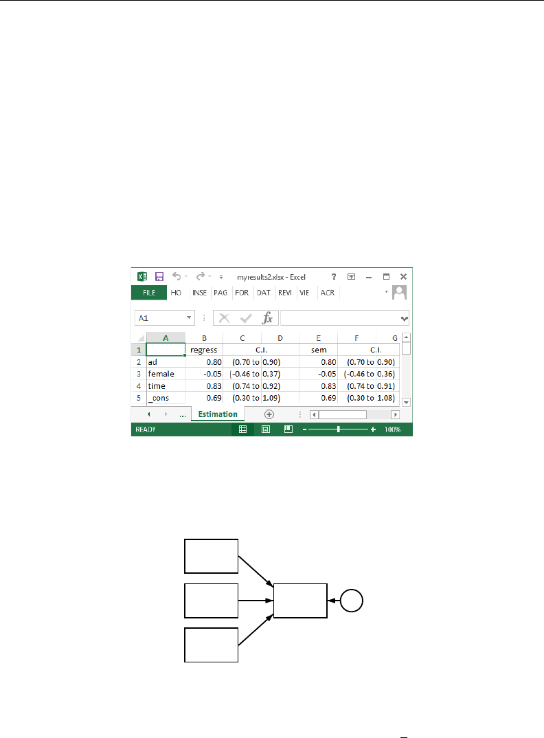
putexcel advanced — Export results to an Excel file using advanced syntax 441
. putexcel E2=matrix(b), nformat(number_d2)
file myresults2.xlsx saved
. putexcel F2=matrix(ll), nformat("(0.00 to;(-0.00 to") right
file myresults2.xlsx saved
. putexcel G2=matrix(ul), nformat("0.00)") left
file myresults2.xlsx saved
Because we are adding estimation results, we change “Coef.” to “regress” and add a column
heading for “sem”. As before, we include a merged column heading for the confidence interval. We
center all column headings by using the hcenter option.
. putexcel B1="regress" E1="sem" F1="C.I.", hcenter
file myresults2.xlsx saved
. putexcel (F1:G1), merge
file myresults2.xlsx saved
Our table from example 3 now includes additional columns for our sem results:
We might also want to export the path diagram for our model so that we can view it while looking
at our results.
visits ε1
ad
female
time
The SEM Builder will allow you to save your path diagram as a PNG file, in addition to other file
types; PNGs can be exported to Excel. We name our path diagram visits sem and save it as a PNG,
and we then output the file to Excel with the picture() output type.

442 putexcel advanced — Export results to an Excel file using advanced syntax
. putexcel B6 = picture(visits_sem.png)
file myresults2.xlsx saved
This adds the path diagram with the upper-left corner aligned in the upper-left corner of cell B6.
Technical note
See the technical notes Excel data size limits and Dates and times in [D]import excel.
References
Crow, K. 2013. Export tables to Excel. The Stata Blog: Not Elsewhere Classified.
http://blog.stata.com/2013/09/25/export-tables-to-excel/.
Gallup, J. L. 2012. A new system for formatting estimation tables.Stata Journal 12: 3–28.
Quint´
o, L. 2012. HTML output in Stata.Stata Journal 12: 702–717.
Also see
[P]putexcel — Export results to an Excel file
[P]postfile — Post results in Stata dataset
[P]return — Return stored results
[D]export — Overview of exporting data from Stata
[D]import — Overview of importing data into Stata
[M-5]docx*( ) — Generate Office Open XML (.docx) file
[M-5]xl( ) — Excel file I/O class

Title
quietly — Quietly and noisily perform Stata command
Description Syntax Remarks and examples Also see
Description
quietly suppresses all terminal output for the duration of command. It is useful both interactively
and in programs.
noisily turns back on terminal output, if appropriate, for the duration of command. It is useful
only in programs.
set output specifies the output to be displayed. It is useful only in programs and even then is
seldom used.
Syntax
Perform command but suppress terminal output
quietly :command
Perform command and ensure terminal output
noisily :command
Specify type of output to display
set output proc |inform |error
Remarks and examples
Remarks are presented under the following headings:
quietly used interactively
quietly used in programs
Note for programmers
quietly used interactively
Example 1
quietly is useful when you are using Stata interactively and want to temporarily suppress the
terminal output. For instance, to estimate a regression of mpg on the variables weight,foreign,
and headroom and to suppress the terminal output, type
. use http://www.stata-press.com/data/r14/auto
(1978 Automobile Data)
. quietly regress mpg weight foreign headroom
.
Admittedly, it is unlikely that you would ever want to do this in real life.
443

444 quietly — Quietly and noisily perform Stata command
quietly used in programs
Technical note
quietly is often used in programs. Say that you have the following program to run a regression
of yon x, calculate the residuals, and then list the outliers, which are defined as points with residuals
below the 5th percentile or above the 95th percentile:
program myprog
regress ‘1’ ‘2’
predict resid, resid
sort resid
summarize resid, detail
list ‘1’ ‘2’ resid if resid< r(p5) | resid> r(p95)
drop resid
end
Although the program will work, it will also fill the screen with the regression output, any notes that
predict feels obligated to mention, and the detailed output from summarize. A better version of
this program might read
program myprog
quietly regress ‘1’ ‘2’
quietly predict resid, resid
quietly sort resid
quietly summarize resid, detail
list ‘1’ ‘2’ resid if resid< r(p5) | resid> r(p95)
drop resid
end
You can also combine quietly with { }:
program myprog
quietly {
regress ‘1’ ‘2’
predict resid, resid
sort resid
summarize resid, detail
}
list ‘1’ ‘2’ resid if resid< r(p5) | resid> r(p95)
drop resid
end
Technical note
noisily is the antonym of quietly, and it too can be used in programs and do-files. In fact,
that is its only real use. We could recode our example program to read as follows:
program myprog
quietly {
regress ‘1’ ‘2’
predict resid, resid
sort resid
summarize resid, detail
noisily list ‘1’ ‘2’ resid if resid< r(p5) | resid> r(p95)
drop resid
}
end
Here we have not improved readability.

quietly — Quietly and noisily perform Stata command 445
Technical note
noisily is not really the antonym of quietly. If the user types quietly myprog yvar xvar,
the output will be suppressed because that is what the user wants. Here a noisily inside myprog
will not display the output—noisily means noisily only if the program was allowed to be noisy
when it was invoked.
Technical note
If you think you understand all this, take the following test. Is there any difference between
quietly do filename and run filename? How about noisily run filename and do filename? What
would happen if you typed quietly noisily summarize myvar? If you typed noisily quietly
summarize myvar?
When you are ready, we will tell you the answers.
quietly do filename is equivalent to run filename. Typing run is easier, however.
noisily run filename is not at all the same as do filename.run produces no output, and no
matter how noisily you run run, it is still quiet.
Typing quietly noisily summarize myvar is the same as typing summarize myvar. Think of
it as quietly {noisily summarize myvar}. It is the inside noisily that takes precedence.
Typing noisily quietly summarize myvar is the same as typing quietly summarize myvar — it
does nothing but burn computer time. Again it is the inside term, quietly this time, that takes
precedence.
Technical note
set output proc means that all output, including procedure (command) output, is displayed.
inform suppresses procedure output but displays informative messages and error messages. error
suppresses all output except error messages. In practice, set output is seldom used.
Note for programmers
If you write a program or ado-file, say, mycmd, there is nothing special you need to do so that your
command can be prefixed with quietly. That said, c-class value c(noisily) (see [P]creturn) will
return 0if output is being suppressed and 1otherwise. Thus your program might read
program mycmd
...
display ...
display ...
...
end

446 quietly — Quietly and noisily perform Stata command
or
program mycmd
...
if c(noisily) {
display ...
display ...
}
...
end
The first style is preferred. If the user executes quietly mycmd, the output from display itself,
along with the output of all other commands, will be automatically suppressed.
If the program must work substantially to produce what is being displayed, however, and the only
reason for doing that work is because of the display, then the second style is preferred. In such cases,
you can include the extra work within the block of code executed only when c(noisily) is true
and thus make your program execute more quickly when it is invoked quietly.
Also see
[P]capture — Capture return code
[U] 18 Programming Stata

Title
return — Preserve stored results
Description Syntax Option Remarks and examples Stored results Also see
Description
return sets aside and restores the contents of r().
return hold stores under name the contents of r() and clears r(). If name is a name
obtained from tempname,name will be dropped automatically at the program’s conclusion, if it is
not automatically or explicitly dropped before that.
return restore restores from name the contents of r() and, unless option hold is specified,
drops name.
return drop removes from memory (drops) name or, if all is specified, all return names
currently saved.
return dir lists the names currently set aside by return.
Syntax
Set aside contents of r()
return hold name
Restore contents of r() from name
return restore name , hold
Drop specified return name
return drop name |all
List names currently stored by return
return dir
Option
hold, specified with return restore, specifies that results continue to be held so that they can be
return restored later, as well. If the option is not specified, the specified results are restored
and name is dropped.
447

448 return — Preserve stored results
Remarks and examples
return is rarely necessary. Most programs open with
program example
version 14.1
syntax . . .
marksample touse
if ‘"‘exp’"’ != "" {
touse e
qui generate double ‘e’ = ‘exp’ if ‘touse’
}
. . . (code to calculate final results). . .
end
In the program above, no commands are given that change the contents of r() until all parsing
is complete and the if exp and =exp are evaluated. Thus the user can type
. summarize myvar
. example . . . if myvar>r(mean) . . .
and the results will be as the user expects.
Some programs, however, have nonstandard and complicated syntax, and in the process of
deciphering that syntax, other r-class commands might be run before the user-specified expressions
are evaluated. Consider a command that reads
program example2
version 14.1
. . . (commands that parse). . .
. . . (r() might be reset at this stage). . .
. . . commands that evaluate user-specified expressions. . .
tempvar touse
mark ‘touse’ ‘if’
tempvar v1 v2
generate double ‘v1’ = ‘exp1’ if ‘touse’
// ‘exp1’ specified by user
generate double ‘v2’ = ‘exp2’ if ‘touse’
// ‘exp2’ specified by user
. . . (code to calculate final results). . .
end
Here it would be a disaster if the user typed
. summarize myvar
. example2 . . . if myvar>r(mean) . . .
because r(mean) would not mean what the user expected it to mean, which is the mean of myvar.
The solution to this problem is to code the following:

return — Preserve stored results 449
program example2
version 14.1
// hold on to r()
tempname myr
_return hold ‘myr’
. . . (commands that parse). . .
. . . (r() might be reset at this stage). . .
. . . commands that evaluate user-specified expressions. . .
// restore r()
_return restore ‘myr’
tempvar touse
mark ‘touse’ ‘if’
tempvar v1 v2
generate double ‘v1’ = ‘exp1’ if ‘touse’
// ‘exp1’ specified by user
generate double ‘v2’ = ‘exp2’ if ‘touse’
// ‘exp2’ specified by user
. . . (code to calculate final results). . .
end
In the above example, we hold on to the contents of r() in ‘myr’ and then later bring them back.
Stored results
return restore restores in r() those results that were stored in r() when return hold was
executed.
Also see
[P]return — Return stored results

Title
return — Return stored results
Description Syntax Options Remarks and examples Also see
Description
Results of calculations are stored by many Stata commands so that they can be easily accessed and
substituted into subsequent commands. This entry summarizes for programmers how to store results.
If your interest is in using previously stored results, see [R]stored results.
return stores results in r().
ereturn stores results in e().
sreturn stores results in s().
Stata also has the values of system parameters and certain constants such as pi stored in c().
Because these values may be referred to but not assigned, the c-class is discussed in a different entry;
see [P]creturn.
Syntax
Return results for general commands, stored in r()
return list , all
return clear
return scalar name =exp
return local name =exp
return local name "string"
return matrix name =matname , copy
return add
450

return — Return stored results 451
Return results for estimation commands, stored in e()
ereturn list , all
ereturn clear
ereturn post bVCns weight , depname(string) obs(#) dof(#)
esample(varname) properties(string)
ereturn scalar name =exp
ereturn local name =exp
ereturn local name "string"
ereturn matrix name =matname , copy
ereturn repost b = b V = V Cns = Cns weight , esample(varname)
properties(string) rename
Return results for parsing commands, stored in s()
sreturn list
sreturn clear
sreturn local name =exp
sreturn local name "string"
where b,V, and Cns are matnames, which is the name of an existing matrix.
fweights, aweights, iweights, and pweights are allowed; see [U] 11.1.6 weight.
Options
all is for use with return list and ereturn list.all specifies that hidden and historical stored
results be listed along with the usual stored results. This option is seldom used. See Using hidden
and historical stored results and Programming hidden and historical stored results in Remarks
and examples for more information. These sections are written in terms of return list, but
everything said there applies equally to ereturn list.
all is not allowed with sreturn list because s() does not allow hidden or historical results.
copy specified with return matrix or ereturn matrix indicates that the matrix is to be copied;
that is, the original matrix should be left in place. The default is to “steal” or “rename” the existing
matrix, which is fast and conserves memory.
depname(string)is for use with ereturn post. It supplies the name of the dependent variable to
appear in the estimation output. The name specified need not be the name of an existing variable.

452 return — Return stored results
obs(#)is for use with ereturn post. It specifies the number of observations on which the estimation
was performed. This number is stored in e(N), and obs() is provided simply for convenience.
Results are no different from those for ereturn post followed by ereturn scalar N = #.
dof(#)is for use with ereturn post. It specifies the number of denominator degrees of freedom to be
used with tand Fstatistics and so is used in calculating significance levels and confidence intervals.
The number specified is stored in e(df r), and dof() is provided simply for convenience. Results
are no different from those for ereturn post followed by ereturn scalar df r = #.
esample(varname)is for use with ereturn post and ereturn repost. It specifies the name of
a 0/1 variable that is to become the e(sample) function. varname must contain 0 and 1 values
only, with 1 indicating that the observation is in the estimation subsample. ereturn post and
ereturn repost will be able to execute a little more quickly if varname is stored as a byte
variable.
varname is dropped from the dataset, or more correctly, it is stolen and stashed in a secret place.
properties(string)specified with ereturn post or ereturn repost sets the e(properties)
macro. By default, e(properties) is set to b V if properties() is not specified.
rename is for use with the b = bsyntax of ereturn repost. All numeric estimation results remain
unchanged, but the labels of bare substituted for the variable and equation names of the already
posted results.
Remarks and examples
Remarks are presented under the following headings:
Introduction
Storing results in r()
Storing results in e()
Storing results in s()
Recommended names for stored results
Using hidden and historical stored results
Programming hidden and historical stored results
Introduction
This entry summarizes information that is presented in greater detail in other parts of the Stata
documentation. Most particularly, we recommend that you read [U] 18 Programming Stata. The
commands listed above are used by programmers to store results, which are accessed by others using
r(),e(), and s(); see [R]stored results.
The commands listed above may be used only in programs—see [U] 18 Programming Stata and
[P]program—and then only when the program is declared explicitly as being rclass,eclass, or
sclass:
program . . ., rclass
. . .
return . . .
. . .
end
program . . ., eclass
. . .
ereturn . . .
. . .
end

return — Return stored results 453
program . . ., sclass
. . .
sreturn . . .
. . .
end
Storing results in r()
•The program must be declared explicitly to be r-class: program . . . , rclass.
•Distinguish between r() (returned results) and return() (results being assembled that will
be returned). The program you write actually stores results in return(). Then when your
program completes, whatever is in return() is copied to r(). Thus the program you write
can consume r() results from other programs, and there is no conflict.
•return clear clears the return() class. This command is seldom used because return()
starts out empty when your program begins. return clear is for those instances when you
have started assembling results and all is going well, but given the problem at hand, you need
to start all over again.
•return scalar name =exp evaluates exp and stores the result in the scalar return(name).
exp must evaluate to a numeric result or missing. If your code has previously stored something
in return(name), whether a scalar, matrix, or whatever else, the previous value is discarded
and this result replaces it.
•return local name =exp evaluates exp and stores the result in the macro return(name).
exp may evaluate to a numeric or string result. If your code has previously stored something
in return(name), whether a scalar, matrix, or whatever else, the previous value is discarded
and this result replaces it.
Be careful with this syntax: do not code
return local name = ‘mymacro’
because that will copy just the first 2045 characters of ‘mymacro’. Instead, code
return local name ‘"‘mymacro’"’
•return local name string copies string to macro return(name). If your code has previously
stored something in return(name), whether a scalar, matrix, or whatever else, the previous
value is discarded and this result replaces it.
If you do not enclose string in double quotes, multiple blanks in string are compressed into
single blanks.
•return matrix name matname destructively copies matname into matrix return(name),
meaning that matname is erased (matname is renamed return(name)). If your code has
previously stored something in return(name), whether a scalar, matrix, or whatever else, the
previous value is discarded and this result replaces it.
•return add copies everything new in r() into return(). Say that your program performed
asummarize.return add lets you add everything just returned by summarize to the to-be-
returned results of your program. If your program had already set return(N),summarize’s
r(N) would not replace the previously set result. The remaining r() results set by summarize
would be copied.

454 return — Return stored results
Storing results in e()
For detailed guidance on storing in e(), see [P]ereturn. What follows is a summary.
•The program must be declared explicitly to be e-class: program . . . , eclass.
•The e-class is cleared whenever an ereturn post is executed. The e-class is a static, single-level
class, meaning that results are posted to the class the instant that they are stored.
•ereturn clear clears e(). This is a rarely used command.
•ereturn post is how you must begin storing results in e(). Because ereturn post clears
e(), anything stored in e() prior to the ereturn post is lost.
ereturn post stores matrix (vector, really) e(b), matrices e(V) and e(Cns), weight-related
macros e(wtype) and e(wexp), and function e(sample). The most common syntax is
ereturn post ‘b’ ‘V’, esample(‘touse’) . . .
where ‘b’ is a row vector containing the parameter estimates, ‘V’ is a symmetric matrix
containing the variance estimates, and ‘touse’ is a 0/1 variable recording 1 in observations
that appear in the estimation subsample.
The result of this command will be that ‘b’,‘V’, and ‘touse’ all disappear. In fact, ereturn
post examines what you specify and, if it is satisfied with them, renames them e(b),e(V),
and e(sample).
For more advanced usage that also posts constraint and weight information, see [P]ereturn.
In terms of ereturn post’s other options,
a. We recommend that you specify depname(string)if there is one dependent variable name
that you want to appear on the output. Whether you specify depname() or not, remember
later to define macro e(depvar) to contain the names of the dependent variables.
b. Specify obs(#), or remember later to define scalar e(N) to contain the number of
observations.
c. Few models require specifying dof(#), or, if that is not done, remembering to later define
scalar e(df r). This all has to do with substituting tand Fstatistics on the basis of
#(denominator) degrees of freedom for asymptotic zand χ2statistics in the estimation
output.
•ereturn scalar name =exp evaluates exp and stores the result in the scalar e(name).exp
must evaluate to a numeric result or missing. If your code has previously stored something in
e(name), whether that be a scalar, matrix, or whatever else, the previous value is discarded
and this result replaces it.
•ereturn local name =exp evaluates exp and stores the result in the macro e(name).exp
may evaluate to a numeric or string result. If your code has previously stored something in
e(name), whether that be a scalar, matrix, or whatever else, the previous value is discarded
and this result replaces it.
Be careful with this syntax: do not code
ereturn local name = ‘mymacro’
because that will copy just the first 2045 characters of ‘mymacro’. Instead, code
ereturn local name ‘"‘mymacro’"’
•ereturn local name string copies string to macro e(name). If your code has previously
stored something in e(name), whether a scalar, matrix, or whatever else, the previous value is
discarded and this result replaces it.

return — Return stored results 455
If you do not enclose string in double quotes, multiple blanks in string are compressed into
single blanks.
•ereturn matrix name =matname destructively copies matname into matrix e(name), meaning
that matname is erased. At least, that is what happens if you do not specify the copy option.
What actually occurs is that matname is renamed e(name). If your code has previously stored
something in e(name), whether a scalar, matrix, or whatever else, the previous value is discarded
and this result replaces it, with two exceptions:
ereturn matrix cannot be used to store in e(b) or e(V). The only way to post matrices to
these special names is to use ereturn post and ereturn repost so that various tests can
be run on them before they are made official. Other Stata commands use e(b) and e(V) and
expect to see a valid estimation result. If e(b) is 1 ×k, they expect e(V) to be k×k. They
expect that the names of rows and columns will be the same so that the ith column of e(b)
corresponds to the ith row and column of e(V). They expect e(V) to be symmetric. They
expect e(V) to have positive or zero elements along its diagonal, and so on. ereturn post
and ereturn repost check these assumptions.
•ereturn repost allows changing e(b),e(V),e(Cns),e(wtype),e(wexp),e(properties),
and e(sample) without clearing the estimation results and starting all over again. As with
ereturn post, specified matrices and variables disappear after reposting because they are
renamed e(b),e(V),e(Cns), or e(sample) as appropriate.
•Programmers posting estimation results should remember to store
a. Macro e(cmd), containing the name of the estimation command. Make this the last thing
you store in e().
b. Macro e(cmdline), containing the command the user typed.
c. Macro e(depvar), containing the names of the dependent variables.
d. Scalar e(N), containing the number of observations.
e. Scalar e(df m), containing the model degrees of freedom.
f. Scalar e(df r), containing the denominator degrees of freedom if estimates are nonasymp-
totic; otherwise, do not define this result.
g. Scalar e(ll), containing the log-likelihood value, if relevant.
h. Scalar e(ll 0), containing the log-likelihood value for the constant-only model, if
relevant.
i. Scalar e(chi2), containing the χ2test of the model against the constant-only model, if
relevant.
j. Macro e(chi2type), containing LR,Wald, or other, depending on how e(chi2) was
obtained.
k. Scalar e(r2), containing the value of the R2if it is calculated.
l. Scalar e(r2 p), containing the value of the pseudo-R2if it is calculated.
m. Macro e(vce), containing the name of the vcetype that was specified in the vce()
option; see [R]vce option.
n. Macro e(vcetype), containing the text to appear above standard errors in estimation
output, typically Robust, or it is undefined.
o. Macro e(clustvar), containing the name of the cluster variable, if any.
p. Scalar e(N clust), containing the number of clusters.
q. Scalar e(rank), containing the rank of e(V).
r. Macro e(predict), containing the name of the command that predict is to use; if this
is blank, predict uses the default predict.

456 return — Return stored results
s. Macro e(estat cmd), containing the name of an estat handler program if you wish
to customize the behavior of estat.
t. Macro e(properties), containing properties of the estimation command, typically b V,
indicating that the command produces a legitimate coefficient vector and VCE matrix.
Storing results in s()
•The program must be declared explicitly to be s-class: program . . . , sclass.
•The s-class is not cleared automatically. It is a static, single-level class. Results are posted to
s() the instant they are stored.
•sreturn clear clears s(). We recommend that you use this command near the top of s-class
routines. sreturn clear may be used in non–s-class programs, too.
•The s-class provides macros only and is intended for returning results of subroutines that parse
input. At the parsing step, it is important that the r-class not be changed or cleared because
some of what still awaits being parsed might refer to r(), and the user expects those results
to substitute according to what was in r() when he or she typed the command.
•sreturn local name =exp evaluates exp and stores the result in the macro s(name).exp
may evaluate to a numeric or string result. If your code has previously stored something else
in s(name), the previous value is discarded and this result replaces it.
Be careful with this syntax: do not code
sreturn local name = ‘mymacro’
because that will copy just the first 2045 characters of ‘mymacro’. Instead, code
sreturn local name ‘"‘mymacro’"’
•sreturn local name string copies string to macro s(name). If your code has previously
stored something else in s(name), the previous value is discarded and this result replaces it.
If you do not enclose string in double quotes, multiple blanks in string are compressed into
single blanks.
Recommended names for stored results
Users will appreciate it if you use predictable names for your stored results. We use these rules:
•Mathematical and statistical concepts such as number of observations and degrees of freedom
are given short mathematical-style names. Subscripting is indicated with ‘ ’. Names are to
proceed from the general to the specific. If Nmeans number of observations, N 1 might be the
number of observations in the first group.
Suffixes are to be avoided where possible. For instance, a χ2statistic would be recorded in
a variable starting with chi2. If, in the context of the command, a statement about “the χ2
statistic” would be understood as referring to this statistic, then the name would be chi2. If
it required further modification, such as χ2for the comparison test, then the name might be
chi2 c.

return — Return stored results 457
Common prefixes are
Nnumber of observations
df degrees of freedom
kcount of parameters
ngeneric count
lb and ub lower and upper bound of confidence interval
chi2 χ2statistic
ttstatistic
FFstatistic
psignificance
pand pr probability
ll log likelihood
Ddeviance
r2 R2
•Programming concepts, such as lists of variable names, are given English-style names. Names
should proceed from the specific to the general. The name of the dependent variable is depvar,
not vardep.
Some examples are
depvar dependent variable names
eqnames equation names
model name of model fit
xvar xvariable
title title used
•Popular usage takes precedence over the rules. For example:
a. mss is model sum of squares, even though, per the first rule of this section, it ought to
be ss m.
b. mean is used as the prefix to record means.
c. Var is used as the prefix to mean variance.
d. The returned results from most Stata commands follow this rule.
Using hidden and historical stored results
Most results stored in r() and e() are visible—type return list. Sometimes, other stored results
exist, too. For instance, consider the Stata command summarize. Let’s pretend that in addition to
everything that summarize stores in r()—you know about r(N),r(mean),r(sd), etc.—summarize
also stores r(secret) and r(sigma).summarize does not do this, but pretend that it did. If
summarize stored r(secret) as hidden and r(sigma) as historical, you would not know they
existed from the output of return list unless you typed return list, all. If you typed that
command, you would discover r(secret) and r(sigma), and you might learn from the output that
r(secret) was hidden whereas r(sigma) was historical. The output is trying to tell you 1) the two
stored results exist, 2) you may use them just as you use any other stored result, and 3) the reason
why the two stored results were not listed by default.
There are two reasons why summarize might not store results so that you can see them when
you type return list.
The first reason is that summarize is designed to work tightly with some other Stata subroutine
and is using r() to pass complicated information. The information that is stored is so arcane that
you would not want to read documentation about it. Stata puts such stored results into the hidden
category where you will not see them by default. If you type return list, all and find hidden

458 return — Return stored results
stored results, we recommend that you do not use their contents in your own do- and ado-files.
Because hidden stored results are not documented, their names, contents, and even their existence
could change in future releases.
The other reason summarize might omit a stored result from return list concerns backward
compatibility. Assume that for Stata 4, summarize stored the standard deviation in r(sigma) instead
of r(sd). Assume that the editors at StataCorp decided later that r(sd) would be a better name. The
programmers at StataCorp could not simply change the name from r(sigma) to r(sd), because users
might have already written do- or ado-files before the change. Changing the name could break old do-
and ado-files, and it is a hallmark of Stata that your code will continue to work regardless of how long
ago users wrote it. Thus the programmers at StataCorp could choose to store the standard deviation
in both r(sigma) and r(sd) in all cases, or they could store the standard deviation in r(sd) and
store it in r(sigma) only when the old do- or ado-file explicitly included a version 4 or earlier
statement. Either way, r(sigma) is of no interest to modern Stata users, and so the programmers mark
r(sigma) as historical. Now when you type return list, you will not see r(sigma) mentioned;
and when you type return list, all, you will see r(sigma) listed, and you are told that it was
not mentioned earlier because it is marked as historical.
Typing return list, all can be useful when you are debugging or adding new features to an
old program and want to see the historical stored results to better understand your old program.
What was just said about r() and return list applies equally to e() and ereturn list, and
it applies equally to user-written additions to Stata and to official Stata commands. That’s the story
of all.
Programmers wishing to exploit the hidden and historical markings in their own programs should
see the next section.
Programming hidden and historical stored results
You can mark stored results as hidden or historical by specifying the optional hcat argument with
the appropriate return or ereturn command:
return hcat scalar name =exp
return hcat local name =exp
return hcat local name "string"
return hcat matrix name =matname , copy
ereturn hcat scalar name =exp
ereturn hcat local name =exp
ereturn hcat local name "string"
ereturn hcat matrix name =matname , copy
hcat specifies the hiddenness of the result and may be
visible
hidden
historical(relno)
where relno is ##.##such as 2,10,10.,10.1, or 10.12.visible is the default when
hcat is not specified.

return — Return stored results 459
Thus if you are writing an r-class command and wish to store r(private) as a hidden scalar,
you can code
return hidden scalar private = . . .
If you wish to store r(lastvar) as a hidden local, you can code
return hidden local lastvar ". . ."
If you wanted r(lastvar) to be historical rather than hidden, you would code
return historical local lastvar ". . ."
If you wanted r(lastvar) to be historical as of Stata 14, meaning that r(lastvar) was current
up to but not including Stata 14, you would code
return historical(14) local lastvar ". . ."
If you wish to create r(X) as a hidden matrix, you can code
return hidden matrix X = . . .
All the above examples could be performed using ereturn instead of return. They could not be
performed using sreturn because s() does not allow hidden or historical results.
The Mata commands for setting r() and e() also allow an optional argument to set hcat; see
[M-5]st numscalar( ),[M-5]st global( ), and [M-5]st matrix( ).
Also see
[P]creturn — Return c-class values
[P]ereturn — Post the estimation results
[P]estimates — Manage estimation results
[P]putexcel — Export results to an Excel file
[P]return — Preserve stored results
[R]stored results — Stored results
[U] 18 Programming Stata
[U] 18.10 Storing results

Title
rmcoll — Remove collinear variables
Description Syntax Options Remarks and examples Stored results Also see
Description
rmcoll returns in r(varlist) an updated version of varlist that is specific to the sample
identified by if,in, and any missing values in varlist.rmcoll flags variables that are to be omitted
because of collinearity. If varlist contains factor variables, then rmcoll also enumerates the levels of
factor variables, identifies the base levels of factor variables, and identifies empty cells in interactions.
The following message is displayed for each variable that rmcoll flags as omitted because of
collinearity:
note: ______ omitted because of collinearity
The following message is displayed for each empty cell of an interaction that rmcoll encounters:
note: ______ identifies no observations in the sample
ml users: it is not necessary to call rmcoll because ml flags collinear variables for you, assuming
that you do not specify ml model’s collinear option. Even so, ml programmers sometimes use
rmcoll because they need the sample-specific set of variables, and in such cases, they specify ml
model’s collinear option so that ml does not waste time looking for collinearity again. See [R]ml.
rmdcoll performs the same task as rmcoll and checks that depvar is not collinear with the
variables in indepvars. If depvar is collinear with any of the variables in indepvars, then rmdcoll
reports the following message with the 459 error code:
______ collinear with ______
Syntax
Identify variables to be omitted because of collinearity
rmcoll varlist if in weight , noconstant collinear expand forcedrop
Identify independent variables to be omitted because of collinearity
rmdcoll depvar indepvars if in weight , noconstant collinear expand
normcoll
varlist and indepvars may contain factor variables; see [U] 11.4.3 Factor variables.
varlist,depvar, and indepvars may contain time-series operators; see [U] 11.4.4 Time-series varlists.
fweights, aweights, iweights, and pweights are allowed; see [U] 11.1.6 weight.
460

rmcoll — Remove collinear variables 461
Options
noconstant specifies that, in looking for collinearity, an intercept not be included. That is, a variable
that contains the same nonzero value in every observation should not be considered collinear.
collinear specifies that collinear variables not be flagged.
expand specifies that the expanded, level-specific variables be posted to r(varlist). This option
will have an effect only if there are factor variables in the variable list.
forcedrop specifies that collinear variables be dropped from the variable list instead of being flagged.
This option is not allowed when the variable list already contains flagged variables, factor variables,
or interactions.
normcoll specifies that collinear variables have already been flagged in indepvars. Otherwise,
rmcoll is called first to flag any such collinearity.
Remarks and examples
rmcoll and rmdcoll are typically used when writing estimation commands.
rmcoll is used if the programmer wants to flag the collinear variables from the independent
variables.
rmdcoll is used if the programmer wants to detect collinearity of the dependent variable with
the independent variables.
Example 1: Flagging variables because of collinearity
Let’s load auto.dta and add a variable called tt that is collinear with variables turn and trunk.
The easiest way to do this is to generate tt as the sum of turn and trunk.
. use http://www.stata-press.com/data/r14/auto
(1978 Automobile Data)
. generate tt = turn + trunk
Now we can use rmcoll to identify that we have a collinearity and flag a variable because of it.
. _rmcoll turn trunk tt
note: tt omitted because of collinearity
. display r(varlist)
turn trunk o.tt
rmcoll reported that tt was being flagged because of collinearity and attached the omit operator
to tt resulting in “o.tt” being returned in r(varlist).
Example 2: Factor variables
rmcoll works with factor variables. Let’s pass rep78 as a factor variable to rmcoll.
. _rmcoll i.rep78
. display r(varlist)
i(1 2 3 4 5)b1.rep78

462 rmcoll — Remove collinear variables
The updated variable list now contains the enumerated levels of rep78 and identifies its base level.
Use the expand option if you want to be able to loop over the level-specific, individual variables in
r(varlist).
. _rmcoll i.rep78, expand
. display r(varlist)
1b.rep78 2.rep78 3.rep78 4.rep78 5.rep78
Example 3: Interactions
rmcoll works with interactions and reports when it encounters empty cells. An empty cell is a
combination of factor levels that does not occur in the dataset. Let’s use the table command with
factor variables rep78 and foreign to see that there are two empty cells:
. table rep78 foreign
Repair
Record Car type
1978 Domestic Foreign
1 2
2 8
3 27 3
4 9 9
5 2 9
Now let’s pass the interaction of factor variables rep78 and foreign to rmcoll.
. _rmcoll rep78#foreign
note: 1.rep78#1.foreign identifies no observations in the sample
note: 2.rep78#1.foreign identifies no observations in the sample
. display r(varlist)
i(1 2 3 4 5)b1o(1 1 2).rep78#i(0 1)b0o(0 1 1).foreign
Example 4: Coding fragment for standard variables
A code fragment for a program that uses rmcoll might read
. . .
syntax varlist [fweight iweight] . . . [, noCONStant . . . ]
marksample touse
if "‘weight’" != "" {
tempvar w
quietly generate double ‘w’ = ‘exp’ if ‘touse’
local wgt [‘weight’=‘w’]
}
else local wgt /* is nothing */
gettoken depvar xvars : varlist
_rmcoll ‘xvars’ ‘wgt’ if ‘touse’, ‘constant’
local xvars ‘r(varlist)’
. . .

rmcoll — Remove collinear variables 463
In this code fragment, varlist contains one dependent variable and zero or more independent
variables. The dependent variable is split off and stored in the local macro depvar. Then the remaining
variables are passed through rmcoll, and the resulting updated independent variable list is stored
in the local macro xvars.
Example 5: Coding fragment for factor variables and time-series operators
Here we modified the above code fragment to allow for factor variables and time-series operators.
. . .
syntax varlist(fv ts) [fweight iweight] . . . [, noCONStant . . . ]
marksample touse
if "‘weight’" != "" {
tempvar w
quietly generate double ‘w’ = ‘exp’ if ‘touse’
local wgt [‘weight’=‘w’]
}
else local wgt /* is nothing */
gettoken depvar xvars : varlist
_rmcoll ‘xvars’ ‘wgt’ if ‘touse’, expand ‘constant’
local xvars ‘r(varlist)’
. . .
The varlist argument in the syntax command contains the fv specifier to allow factor variables
and the ts specifier to allow time-series operators. We also added the expand option in case the
remaining code needs to loop over the level-specific, individual variables in the xvars macro.
Stored results
rmcoll and rmdcoll store the following in r():
Scalars
r(k omitted) number of omitted variables in r(varlist)
Macros
r(varlist) the flagged and expanded variable list
Also see
[R]ml — Maximum likelihood estimation
[U] 18 Programming Stata

Title
rmsg — Return messages
Description Syntax Option Remarks and examples Also see
Description
set rmsg determines whether the return message is to be displayed at the completion of each
command. The initial setting is off. The return message shows how long the command took to
execute and what time it completed execution.
Syntax
set rmsg on |off , permanently
Option
permanently specifies that, in addition to making the change right now, the rmsg setting be
remembered and become the default setting when you invoke Stata.
Remarks and examples
See [U] 8 Error messages and return codes for a description of return messages and for use of
this command.
Also see
[P]error — Display generic error message and exit
[P]timer — Time sections of code by recording and reporting time spent
[R]query — Display system parameters
[U] 8 Error messages and return codes
464

Title
robust — Robust variance estimates
Description Syntax Options Remarks and examples
Stored results Methods and formulas References Also see
Description
robust helps implement estimation commands and is rarely used. That is because other commands
are implemented in terms of it and are easier and more convenient to use. For instance, if all you
want to do is make your estimation command allow the vce(robust) and vce(cluster clustvar)
options, see [R]ml. If you want to make your estimation command work with survey data, it is easier
to make your command work with the svy prefix—see [P]program properties—rather than to use
robust.
If you really want to understand what ml and svy are doing, however, this is the section for you.
Or, if you have an estimation problem that does not fit with the ml or svy framework, then robust
may be able to help.
robust is a programmer’s command that computes a robust variance estimator based on varlist
of equation-level scores and a covariance matrix. It produces estimators for ordinary data (each
observation independent), clustered data (data not independent within groups, but independent across
groups), and complex survey data from one stage of stratified cluster sampling.
The robust variance estimator goes by many names: Huber/White/sandwich are typically used in
the context of robustness against heteroskedasticity. Survey statisticians often refer to this variance
calculation as a first-order Taylor-series linearization method. Despite the different names, the estimator
is the same.
The equation-level score variables (varlist) consist of one variable for single-equation models or
multiple variables for multiple-equation models, one variable for each equation. The “covariance”
matrix before adjustment is either posted using ereturn post (see [P]ereturn) or specified with the
variance(matname)option. In the former case, robust replaces the covariance in the post with
the robust covariance matrix. In the latter case, the matrix matname is overwritten with the robust
covariance matrix. Note: The robust covariance formula is V=DMD, where Dis what we are
calling the “covariance” matrix before adjustment; this is not always a true covariance. See Remarks
and examples below.
Before reading this section, you should be familiar with [U] 20.21 Obtaining robust variance
estimates and the Methods and formulas section of [R]regress. We assume that you have already
programmed an estimator in Stata and now wish to have it compute robust variance estimates. If you
have not yet programmed your estimator, see [U] 18 Programming Stata,[R]ml, and [P]ereturn.
If you wish to program an estimator for survey data, then you should write the estimator for
nonsurvey data first and then use the instructions in [P]program properties (making programs
svyable) to get your estimation command to work properly with the svy prefix. See [SVY]variance
estimation for a discussion of variance estimation for survey data.
465

466 robust — Robust variance estimates
Syntax
robust varlist if in weight , variance(matname) minus(#)
strata(varname) psu(varname) cluster(varname) fpc(varname)
subpop(varname) vsrs(matname) srssubpop zeroweight
robust works with models that have all types of varlists, including those with factor variables and time-series
operators; see [U] 11.4.3 Factor variables and [U] 11.4.4 Time-series varlists.
pweights, aweights, fweights, and iweights are allowed; see [U] 11.1.6 weight.
Options
variance(matname)specifies a matrix containing the unadjusted “covariance” matrix, that is, the
Din V=DMD. The matrix must have its rows and columns labeled with the appropriate
corresponding variable names, that is, the names of the x’s in xβ. If there are multiple equations,
the matrix must have equation names; see [P]matrix rownames. The Dmatrix is overwritten
with the robust covariance matrix V. If variance() is not specified, Stata assumes that Dhas
been posted using ereturn post;robust will then automatically post the robust covariance
matrix Vand replace D.
minus(#)specifies k=#for the multiplier n/(n−k)of the robust variance estimator. Stata’s
maximum likelihood commands use k=1, and so does the svy prefix. regress, vce(robust)
uses, by default, this multiplier with kequal to the number of explanatory variables in the model,
including the constant. The default is k=1. See Methods and formulas for details.
strata(varname)specifies the name of a variable (numeric or string) that contains stratum identifiers.
psu(varname)specifies the name of a variable (numeric or string) that contains identifiers for the
primary sampling unit (PSU). psu() and cluster() are synonyms; they both specify the same
thing.
cluster(varname)is a synonym for psu().
fpc(varname)requests a finite population correction for the variance estimates. If the variable specified
has values less than or equal to 1, it is interpreted as a stratum sampling rate fh=nh/Nh,
where nhis the number of PSUs sampled from stratum hand Nhis the total number of PSUs
in the population belonging to stratum h. If the variable specified has values greater than 1, it is
interpreted as containing Nh.
subpop(varname)specifies that estimates be computed for the single subpopulation defined by the
observations for which varname 6=0 (and is not missing). This option would typically be used
only with survey data; see [SVY]subpopulation estimation.
vsrs(matname)creates a matrix containing b
Vsrswor, an estimate of the variance that would have
been observed had the data been collected using simple random sampling without replacement.
This is used to compute design effects for survey data; see [SVY]estat for details.
srssubpop can be specified only if vsrs() and subpop() are specified. srssubpop requests that
the estimate of simple-random-sampling variance, vsrs(), be computed assuming sampling within
a subpopulation. If srssubpop is not specified, it is computed assuming sampling from the entire
population.
zeroweight specifies whether observations with weights equal to zero should be omitted from the
computation. This option does not apply to frequency weights; observations with zero frequency
weights are always omitted. If zeroweight is specified, observations with zero weights are

robust — Robust variance estimates 467
included in the computation. If zeroweight is not specified (the default), observations with zero
weights are omitted. Including the observations with zero weights affects the computation in that
it may change the counts of PSUs (clusters) per stratum. Stata’s svy prefix command includes
observations with zero weights; all other commands exclude them. This option is typically used
only with survey data.
Remarks and examples
Remarks are presented under the following headings:
Introduction
Clustered data
Survey data
Controlling the header display
Maximum likelihood estimators
Multiple-equation estimators
Introduction
This section explains the formulas behind the robust variance estimator and how to use robust
through an informal development with some simple examples. For an alternative discussion, see
[U] 20.21 Obtaining robust variance estimates. See the references cited at the end of this entry for
more formal expositions.
First, consider ordinary least-squares regression. The estimator for the coefficients is
b
β= (X0X)−1X0y
where yis an n×1 vector representing the dependent variable and Xis an n×kmatrix of covariates.
Because everything is considered conditional on X,(X0X)−1can be regarded as a constant matrix.
Hence, the variance of b
βis
V(b
β) = (X0X)−1V(X0y) (X0X)−1
What is the variance of X0y, a k×1 vector? Look at its first element; it is
X0
1y=x11y1+x21y2+· · · +xn1yn
where X1is the first column of X. Because Xis treated as a constant, you can write the variance as
V(X0
1y) = x2
11V(y1) + x2
21V(y2) + · · · +x2
n1V(yn)
The only assumption made here is that the yjare independent.
The obvious estimate for V(yj)is be2
j, the square of the residual bej=yj−xjb
β, where xjis the
jth row of X. You must estimate the off-diagonal terms of the covariance matrix for X0y, as well.
Working this out, you have
b
V(X0y) =
n
X
j=1 be2
jx0
jxj
xjis defined as a row vector so that x0
jxjis a k×kmatrix.

468 robust — Robust variance estimates
You have just derived the robust variance estimator for linear regression coefficient estimates for
independent observations:
b
V(b
β)=(X0X)−1n
X
j=1 be2
jx0
jxj(X0X)−1
You can see why it is called the sandwich estimator.
Technical note
The only detail not discussed is the multiplier. You will see later that survey statisticians like to
view the center of the sandwich as a variance estimator for totals. They use a multiplier of n/(n−1),
just as 1/(n−1)is used for the variance estimator of a mean. However, for survey data, nis no
longer the total number of observations but is the number of clusters in a stratum. See Methods and
formulas at the end of this entry.
Linear regression is, however, special. Assuming homoskedasticity and normality, you can derive
the expectation of be2
jfor finite n. This is discussed in [R]regress. Under the assumptions of
homoskedasticity and normality, n/(n−k)is a better multiplier than n/(n−1).
If you specify the minus(#)option, robust will use n/(n−#)as the multiplier. regress,
vce(robust) also gives two other options for the multiplier: hc2 and hc3. Because these multipliers
are special to linear regression, robust does not compute them.
Example 1
Before we show how robust is used, let’s compute the robust variance estimator “by hand” for
linear regression for the case in which observations are independent (that is, no clusters).
We need to compute D= (X0X)−1and the residuals bej.regress with the mse1 option will
allow us to compute both easily; see [R]regress.
. use http://www.stata-press.com/data/r14/_robust
(1978 Automobile Data -- modified)
. regress mpg weight gear_ratio foreign, mse1
(output omitted )
. matrix D = e(V)
. predict double e, residual
We can write the center of the sandwich as
M=
n
X
j=1 be2
jx0
jxj=X0WX
where Wis a diagonal matrix with be2
jon the diagonal. matrix accum with iweights can be used
to calculate this (see [P]matrix accum):
. matrix accum M = weight gear_ratio foreign [iweight=e^2]
(obs=813.7814109)

robust — Robust variance estimates 469
We now assemble the sandwich. To match regress, vce(robust), we use a multiplier of n/(n−k).
. matrix V = 74/70 * D*M*D
. matrix list V
symmetric V[4,4]
weight gear_ratio foreign _cons
weight 3.788e-07
gear_ratio .00039798 1.9711317
foreign .00008463 -.55488334 1.4266939
_cons -.00236851 -6.9153285 1.2149035 27.536291
The result is the same as that from regress, vce(robust):
. regress mpg weight gear_ratio foreign, vce(robust)
(output omitted )
. matrix Vreg = e(V)
. matrix list Vreg
symmetric Vreg[4,4]
weight gear_ratio foreign _cons
weight 3.788e-07
gear_ratio .00039798 1.9711317
foreign .00008463 -.55488334 1.4266939
_cons -.00236851 -6.9153285 1.2149035 27.536291
If we use robust, the initial steps are the same. We still need D, the “bread” of the sandwich,
and the residuals. The residuals eare the varlist for robust.Dis passed via the variance()
option (abbreviation v()). Dis overwritten and contains the robust variance estimate.
. drop e
. regress mpg weight gear_ratio foreign, mse1
(output omitted )
. matrix D = e(V)
. predict double e, residual
. _robust e, v(D) minus(4)
. matrix list D
symmetric D[4,4]
weight gear_ratio foreign _cons
weight 3.788e-07
gear_ratio .00039798 1.9711317
foreign .00008463 -.55488334 1.4266939
_cons -.00236851 -6.9153285 1.2149035 27.536291
Rather than specifying the variance() option, we can use ereturn post to post Dand the
point estimates. robust alters the post, substituting the robust variance estimates.
. drop e
. regress mpg weight gear_ratio foreign, mse1
(output omitted )
. matrix D = e(V)
. matrix b = e(b)
. local n = e(N)
. local k = colsof(D)
. local dof = ‘n’ - ‘k’
. predict double e, residual
. ereturn post b D, dof(‘dof’)
. _robust e, minus(‘k’)

470 robust — Robust variance estimates
. ereturn display
Robust
Coef. Std. Err. t P>|t| [95% Conf. Interval]
weight -.006139 .0006155 -9.97 0.000 -.0073666 -.0049115
gear_ratio 1.457113 1.40397 1.04 0.303 -1.343016 4.257243
foreign -2.221682 1.194443 -1.86 0.067 -4.603923 .1605598
_cons 36.10135 5.247503 6.88 0.000 25.63554 46.56717
Again what we did matches regress, vce(robust):
. regress mpg weight gear_ratio foreign, vce(robust)
Linear regression Number of obs = 74
F(3, 70) = 48.30
Prob > F = 0.0000
R-squared = 0.6670
Root MSE = 3.4096
Robust
mpg Coef. Std. Err. t P>|t| [95% Conf. Interval]
weight -.006139 .0006155 -9.97 0.000 -.0073666 -.0049115
gear_ratio 1.457113 1.40397 1.04 0.303 -1.343016 4.257243
foreign -2.221682 1.194443 -1.86 0.067 -4.603923 .1605598
_cons 36.10135 5.247503 6.88 0.000 25.63554 46.56717
Technical note
Note the simple ways in which robust was called. When we used the variance() option, we
called it by typing
. _robust e, v(D) minus(4)
As we described, robust computed
b
V(b
β) = Dn
n−k
n
X
j=1 be2
jx0
jxjD
We passed Dto robust by using the v(D) option and specified bejas the variable e. So how did
robust know what variables to use for xj? It got them from the row and column names of the
matrix D. Recall how we generated Dinitially:
. regress mpg weight gear_ratio foreign, mse1
(output omitted )
. matrix D = e(V)
. matrix list D
symmetric D[4,4]
weight gear_ratio foreign _cons
weight 5.436e-08
gear_ratio .00006295 .20434146
foreign .00001032 -.08016692 .1311889
_cons -.00035697 -.782292 .17154326 3.3988878

robust — Robust variance estimates 471
Stata’s estimation commands and the ml commands produce matrices with appropriately labeled
rows and columns. If that is how we generate our D, this will be taken care of automatically. But if
we generate Din another manner, we must be sure to label it appropriately; see [P]matrix rownames.
When robust is used after ereturn post, it gets the variable names from the row and column
names of the posted matrices. So again, the matrices must be labeled appropriately.
Let us make another rather obvious comment. robust uses the variables from the row and
column names of the Dmatrix at the time robust is called. It is the programmer’s responsibility
to ensure that the data in these variables have not changed and that robust selects the appropriate
observations for the computation, using an if restriction if necessary (for instance, if e(sample)).
Clustered data
Example 2
To get robust variance estimates for clustered data or for complex survey data, simply use the
cluster(),strata(), etc., options when you call robust.
The first steps are the same as before. For clustered data, the number of degrees of freedom of
the tstatistic is the number of clusters minus one (we will discuss this later).
. drop e
. quietly regress mpg weight gear_ratio foreign, mse1
. generate byte samp = e(sample)
. matrix D = e(V)
. matrix b = e(b)
. predict double e, residual
. local k = colsof(D)
. tabulate rep78
Repair
Record 1978 Freq. Percent Cum.
1 2 2.90 2.90
2 8 11.59 14.49
3 30 43.48 57.97
4 18 26.09 84.06
5 11 15.94 100.00
Total 69 100.00
. local nclust = r(r)
. display ‘nclust’
5
. local dof = ‘nclust’ - 1
. ereturn post b D, dof(‘dof’) esample(samp)
. _robust e, minus(‘k’) cluster(rep78)

472 robust — Robust variance estimates
. ereturn display
(Std. Err. adjusted for 5 clusters in rep78)
Robust
Coef. Std. Err. t P>|t| [95% Conf. Interval]
weight -.006139 .0008399 -7.31 0.002 -.008471 -.0038071
gear_ratio 1.457113 1.801311 0.81 0.464 -3.544129 6.458355
foreign -2.221682 .8144207 -2.73 0.053 -4.482876 .0395129
_cons 36.10135 3.39887 10.62 0.000 26.66458 45.53813
What you get is, of course, the same as regress, vce(cluster rep78). Wait a minute. It is not
the same!
. regress mpg weight gear_ratio foreign, vce(cluster rep78)
Linear regression Number of obs = 69
F(3, 4) = 78.61
Prob > F = 0.0005
R-squared = 0.6631
Root MSE = 3.4827
(Std. Err. adjusted for 5 clusters in rep78)
Robust
mpg Coef. Std. Err. t P>|t| [95% Conf. Interval]
weight -.005893 .0008214 -7.17 0.002 -.0081735 -.0036126
gear_ratio 1.904503 2.18322 0.87 0.432 -4.157088 7.966093
foreign -2.149017 1.20489 -1.78 0.149 -5.49433 1.196295
_cons 34.09959 4.215275 8.09 0.001 22.39611 45.80307
Not even the point estimates are the same. This is the classic programmer’s mistake of not using the
same sample for the initial regress, mse1 call as done with robust. The cluster variable rep78
is missing for 5 observations. robust omitted these observations, but regress, mse1 did not.
robust is best used only in programs for just this reason. So, you can write a program and use
marksample and markout (see [P]mark) to determine the sample in advance of running regress
and robust.

robust — Robust variance estimates 473
begin myreg.ado
program myreg, eclass sortpreserve
version 14.1
syntax varlist [if] [in] [, CLuster(varname) ]
marksample touse
markout ‘touse’ ‘cluster’, strok
tempvar e count
tempname D b
quietly {
regress ‘varlist’ if ‘touse’, mse1
matrix ‘D’ = e(V)
matrix ‘b’ = e(b)
local n = e(N)
local k = colsof(‘D’)
predict double ‘e’ if ‘touse’, residual
if "‘cluster’"!="" {
sort ‘touse’ ‘cluster’
by ‘touse’ ‘cluster’: gen byte ‘count’ = 1 if _n==1 & ‘touse’
summarize ‘count’, meanonly
local nclust = r(sum)
local dof = ‘nclust’ - 1
local clopt "cluster(‘cluster’)"
}
else local dof = ‘n’ - ‘k’
ereturn post ‘b’ ‘D’, dof(‘dof’) esample(‘touse’)
_robust ‘e’ if e(sample), minus(‘k’) ‘clopt’
}
ereturn display
end
end myreg.ado
Running this program produces the same results as regress, vce(cluster clustvar).
. myreg mpg weight gear_ratio foreign, cluster(rep78)
(Std. Err. adjusted for 5 clusters in rep78)
Robust
Coef. Std. Err. t P>|t| [95% Conf. Interval]
weight -.005893 .0008214 -7.17 0.002 -.0081735 -.0036126
gear_ratio 1.904503 2.18322 0.87 0.432 -4.157088 7.966093
foreign -2.149017 1.20489 -1.78 0.149 -5.49433 1.196295
_cons 34.09959 4.215275 8.09 0.001 22.39611 45.80307

474 robust — Robust variance estimates
Survey data
Example 3
We will now modify our myreg command so that it handles complex survey data. Our new version
will allow pweights and iweights, stratification, and clustering.
begin myreg.ado
program myreg, eclass
version 14.1
syntax varlist [if] [in] [pweight iweight] [, /*
*/ STRata(varname) CLuster(varname) ]
marksample touse, zeroweight
markout ‘touse’ ‘cluster’ ‘strata’, strok
if "‘weight’"!="" {
tempvar w
quietly generate double ‘w’ ‘exp’ if ‘touse’
local iwexp "[iw=‘w’]"
if "‘weight’" == "pweight" {
capture assert ‘w’ >= 0 if ‘touse’
if c(rc) error 402
}
}
if "‘cluster’"!="" {
local clopt "cluster(‘cluster’)"
}
if "‘strata’"!="" {
local stopt "strata(‘strata’)"
}
tempvar e
tempname D b
quietly {
regress ‘varlist’ ‘iwexp’ if ‘touse’, mse1
matrix ‘D’ = e(V)
matrix ‘b’ = e(b)
predict double ‘e’ if ‘touse’, residual
_robust ‘e’ ‘iwexp’ if ‘touse’, v(‘D’) ‘clopt’ ‘stopt’ zeroweight
local dof = r(N_clust) - r(N_strata)
local depn : word 1 of ‘varlist’
ereturn post ‘b’ ‘D’, depn(‘depn’) dof(‘dof’) esample(‘touse’)
}
display
ereturn display
end
end myreg.ado
Note the following details about our version of myreg for survey data:
•We called robust before we posted the matrices with ereturn post, whereas in our previous
version of myreg, we called ereturn post and then robust. Here we called robust first so
that we could use its r(N strata), containing the number of strata, and r(N clust), containing
the number of clusters; see Stored results at the end of this entry. We did this so that we could
pass the correct degrees of freedom (=number of clusters −number of strata) to ereturn post.
This works even if the strata() and cluster() options are not specified: r(N strata) =1 if
strata() is not specified (there truly is one stratum); and r(N clust) =number of observations
if cluster() is not specified (each observation is a cluster).
•The call to robust was made with iweights, whether myreg was called with pweights
or iweights. Computationally, robust treats pweights and iweights the same. The only
difference is that it puts out an error message if it encounters a negative pweight, whereas

robust — Robust variance estimates 475
negative iweights are allowed. As good programmers, we put out the error message early before
any time-consuming computations are done.
•We used the zeroweight option with the marksample command so that zero weights would not
be excluded from the sample. We gave the zeroweight option with robust so that it, too,
would not exclude zero weights.
Observations with zero weights affect results only by their effect (if any) on the counts of the clusters.
Setting some weights temporarily to zero will, for example, produce subpopulation estimates. If
subpopulation estimates are desired, however, it would be better to implement robust’s subpop()
option and restrict the call to regress, mse1 to this subpopulation.
•Stata’s svyset accepts a psu variable rather than having a cluster() option. This is only a
matter of style. They are synonyms, as far as robust is concerned.
Our program gives the same results as svy: regress. For our example, we add a strata variable
and a psu variable to the auto dataset.
. use http://www.stata-press.com/data/r14/auto, clear
(1978 Automobile Data)
. set seed 1
. generate strata = int(3*runiform()) + 1
. generate psu = int(5*runiform()) + 1
. myreg mpg weight gear_ratio foreign [pw=displ], strata(strata) cluster(psu)
mpg Coef. Std. Err. t P>|t| [95% Conf. Interval]
weight -.0057248 .000388 -14.75 0.000 -.0065702 -.0048794
gear_ratio .7775839 1.20131 0.65 0.530 -1.839845 3.395013
foreign -1.86776 1.122833 -1.66 0.122 -4.314202 .5786828
_cons 36.64061 3.844625 9.53 0.000 28.26389 45.01733
. svyset psu [pw=displ], strata(strata)
pweight: displacement
VCE: linearized
Single unit: missing
Strata 1: strata
SU 1: psu
FPC 1: <zero>
. svy: regress mpg weight gear_ratio foreign
(running regress on estimation sample)
Survey: Linear regression
Number of strata = 3 Number of obs = 74
Number of PSUs = 15 Population size = 14,600
Design df = 12
F( 3, 10) = 68.37
Prob > F = 0.0000
R-squared = 0.6900
Linearized
mpg Coef. Std. Err. t P>|t| [95% Conf. Interval]
weight -.0057248 .000388 -14.75 0.000 -.0065702 -.0048794
gear_ratio .7775839 1.20131 0.65 0.530 -1.839845 3.395013
foreign -1.86776 1.122833 -1.66 0.122 -4.314202 .5786828
_cons 36.64061 3.844625 9.53 0.000 28.26389 45.01733

476 robust — Robust variance estimates
Controlling the header display
Example 4
Let’s compare the output for our survey version of myreg with the earlier version that handled
only clustering. The header for the earlier version was
(Std. Err. adjusted for 5 clusters in rep78)
Robust
Coef. Std. Err. t P>|t| [95% Conf. Interval]
The header for the survey version lacked the word “Robust” above “Std. Err.”, and it lacked the
banner “(Std. Err. adjusted for #clusters in varname)”.
Both of these headers were produced by ereturn display, and programmers can control what
it produces. The word above “Std. Err.” is controlled by setting e(vcetype). The banner “(Std. Err.
adjusted for #clusters in varname)” is controlled by setting e(clustvar) to the cluster variable
name. These can be set using the ereturn local command; see [P]ereturn.
When robust is called after ereturn post (as it was in the earlier version that produced the
above header), it automatically sets these macros. To not display the banner, the code should read
ereturn post ...
_robust ...
ereturn local clustvar ""
We can also change the phrase displayed above “Std. Err.” by resetting e(vcetype). To display
nothing there, reset e(vcetype) to empty—ereturn local vcetype "".
For our survey version of myreg, we called robust before calling ereturn post. Here robust
does not set these macros. Trying to do so would be futile because ereturn post clears all previous
estimation results, including all e() macros, but you can set them yourself after calling ereturn
post. We make this addition to our survey version of myreg:
_robust ...
ereturn post ...
ereturn local vcetype "Design-based"
The output is
. myreg mpg weight gear_ratio foreign [pw=displ], strata(strata) cluster(psu)
mpg Coef. Std. Err. t P>|t| [95% Conf. Interval]
weight -.0057248 .000388 -14.75 0.000 -.0065702 -.0048794
gear_ratio .7775839 1.20131 0.65 0.530 -1.839845 3.395013
foreign -1.86776 1.122833 -1.66 0.122 -4.314202 .5786828
_cons 36.64061 3.844625 9.53 0.000 28.26389 45.01733

robust — Robust variance estimates 477
Maximum likelihood estimators
Maximum likelihood estimators are basically no different from linear regression when it comes to
the use of robust. We will first do a little statistics and then give a simple example.
We can write our maximum-likelihood estimation equation as
G(β) =
n
X
j=1
S(β;yj,xj) = 0
where S(β;yj,xj) = ∂lnLj/∂βis the score and lnLjis the log likelihood for the jth observation.
Here βrepresents all the parameters in the model, including any auxiliary parameters. We will discuss
how to use robust when there are auxiliary parameters or multiple equations in the next section.
But for now, all the theory works out fine for any set of parameters.
Using a first-order Taylor-series expansion (that is, the delta method), we can write the variance
of G(β)as
b
V{G(β)}β=b
β=∂G(β)
∂ββ=b
βb
V(b
β)∂G(β)
∂β0β=b
β
Solving for b
V(b
β)gives
b
V(b
β) = "∂G(β)
∂β−1
b
V{G(β)}∂G(β)
∂β0−1#β=b
β
but
H=∂G(β)
∂β
is the Hessian (matrix of second derivatives) of the log likelihood. Thus we can write
b
V(b
β) = Db
V{G(β)}β=b
βD
where D=−H−1is the traditional covariance estimate.
Now G(β)is simply a sum, and we can estimate its variance just as we would the sum of any
other variable—it is n2times the standard estimator of the variance of a mean:
n
n−1
n
X
j=1
(zj−z)2
But here, the scores uj=S(b
β;yj,xj)are (row) vectors. Their sum, and thus their mean, is zero.
So, we have
b
V{G(β)}β=b
β=n
n−1
n
X
j=1
u0
juj
Thus our robust variance estimator is
b
V(b
β) = Dn
n−1
n
X
j=1
u0
jujD

478 robust — Robust variance estimates
so we see that the robust variance estimator is just the delta method combined with a simple estimator
for totals!
The above estimator for the variance of the total (the center of the sandwich) is appropriate only
when observations are independent. For clustered data and complex survey data, this estimator is
replaced by one appropriate for the independent units of the data. Clusters (or PSUs) are independent,
so we can sum the scores within a cluster to create a “superobservation” and then use the standard
formula for a total on these independent superobservations. Our robust variance estimator thus becomes
b
V(b
β) = Dnc
nc−1
nc
X
i=1X
j∈Ci
uj0X
j∈Ci
ujD
where Cicontains the indices of the observations belonging to the ith cluster for i=1,2, . . . , nc,
with ncthe total number of clusters.
See [SVY]variance estimation for the variance estimator for a total that is appropriate for complex
survey data. Our development here has been heuristic. We have, for instance, purposefully omitted
sampling weights from our discussion; see [SVY]variance estimation for a better treatment.
See Gould, Pitblado, and Poi (2010) for a discussion of maximum likelihood and of Stata’s ml
command.
Technical note
It is easy to see where the appropriate degrees of freedom for the robust variance estimator come
from: the center of the sandwich is n2times the standard estimator of the variance for the mean of n
observations. A mean divided by its standard error has exactly a Student’s tdistribution with n−1
degrees of freedom for normal i.i.d. variables but also has approximately this distribution under many
other conditions. Thus a point estimate divided by the square root of its robust variance estimate is
approximately distributed as a Student’s twith n−1 degrees of freedom.
More importantly, this also applies to clusters, where each cluster is considered a “superobservation”.
Here the degrees of freedom is nc−1, where ncis the number of clusters (superobservations). If
there are only a few clusters, confidence intervals using tstatistics can become quite large. It is just
like estimating a mean with only a few observations.
When there are strata, the degrees of freedom is nc−L, where Lis the number of strata; see
[SVY]variance estimation for details.
Not all of Stata’s maximum likelihood estimators that produce robust variance estimators for
clustered data use tstatistics. Obviously, this matters only when the number of clusters is small.
Users who want to be rigorous in handling clustered data should use the svy prefix, which always
uses tstatistics and adjusted Wald tests (see [R]test). Programmers who want to impose similar rigor
should do likewise.
We have not yet given any details about the functional form of our scores uj=∂lnLj/∂β. The
log likelihood lnLjis a function of xjβ(the “index”). Logistic regression, probit regression, and
Poisson regression are examples. There are no auxiliary parameters, and there is only one equation.
We can then write uj=bsjxj, where
bsj=∂lnLj
∂(xjβ)β=b
β

robust — Robust variance estimates 479
We refer to sjas the equation-level score. Our formula for the robust estimator when observations
are independent becomes
b
V(b
β) = Dn
n−1
n
X
j=1 bs2
jx0
jxjD
This is precisely the formula that we used for linear regression, with bejreplaced by bsjand k=1
in the multiplier.
Before we discuss auxiliary parameters, let’s show how to implement robust for single-equation
models.
Example 5
The robust variance implementation for single-equation maximum-likelihood estimators with no
auxiliary parameters is almost the same as it is for linear regression. The only differences are that Dis
now the traditional covariance matrix (the negative of the inverse of the matrix of second derivatives)
and that the variable passed to robust is the equation-level score bsjrather than the residuals bej.
Let’s alter our last myreg program for survey data to make a program that does logistic regression
for survey data. We have to change only a few lines of the program.
begin mylogit.ado
program mylogit, eclass
version 14.1
syntax varlist [if] [in] [pweight] [, /*
*/ STRata(varname) CLuster(varname) ]
marksample touse, zeroweight
markout ‘touse’ ‘strata’ ‘cluster’, strok
if "‘weight’"!="" {
tempvar w
quietly generate double ‘w’ ‘exp’ if ‘touse’
local iwexp "[iw=‘w’]"
capture assert ‘w’ >= 0 if ‘touse’
if c(rc) error 402
}
if "‘cluster’"!="" {
local clopt "cluster(‘cluster’)"
}
if "‘strata’"!="" {
local stopt "strata(‘strata’)"
}
tempvar s
tempname D b
quietly {
logit ‘varlist’ ‘iwexp’ if ‘touse’
matrix ‘D’ = e(V)
matrix ‘b’ = e(b)
predict double ‘s’ if e(sample), score
_robust ‘s’ ‘iwexp’ if e(sample), v(‘D’) ‘clopt’ ‘stopt’ zeroweight
local dof = r(N_clust) - r(N_strata)
local depn : word 1 of ‘varlist’
replace ‘touse’ = e(sample)
ereturn post ‘b’ ‘D’, depn(‘depn’) dof(‘dof’) esample(‘touse’)
ereturn local vcetype "Design-based"
}
display
ereturn display
end
end mylogit.ado

480 robust — Robust variance estimates
Note the following about our program:
•We use the score option of predict after logit to obtain the equation-level scores. If predict
does not have a score option, then we must generate the equation-level score variable some other
way.
•logit is a unique command in that it will sometimes drop observations for reasons other than
missing values (for example, when success or failure is predicted perfectly), so our ‘touse’
variable may not represent the true estimation sample. That is why we used the if e(sample)
condition with the predict and robust commands. Then, to provide ereturn post with an
appropriate esample() option, we set the ‘touse’ variable equal to the e(sample) from the
logit command and then use this ‘touse’ variable in the esample() option.
Our mylogit program gives the same results as svy: logit:
. mylogit foreign mpg weight gear_ratio [pw=displ], strata(strata) cluster(psu)
Design-based
foreign Coef. Std. Err. t P>|t| [95% Conf. Interval]
foreign
mpg -.3489011 .1258802 -2.77 0.017 -.6231705 -.0746317
weight -.0040789 .0012508 -3.26 0.007 -.0068042 -.0013536
gear_ratio 6.324169 1.729436 3.66 0.003 2.556051 10.09229
_cons -2.189748 7.75427 -0.28 0.782 -19.08485 14.70536
. svyset psu [pw=displ], strata(strata)
pweight: displacement
VCE: linearized
Single unit: missing
Strata 1: strata
SU 1: psu
FPC 1: <zero>
. svy: logit foreign mpg weight gear_ratio
(running logit on estimation sample)
Survey: Logistic regression
Number of strata = 3 Number of obs = 74
Number of PSUs = 15 Population size = 14,600
Design df = 12
F( 3, 10) = 6.89
Prob > F = 0.0085
Linearized
foreign Coef. Std. Err. t P>|t| [95% Conf. Interval]
mpg -.3489011 .1258802 -2.77 0.017 -.6231705 -.0746317
weight -.0040789 .0012508 -3.26 0.007 -.0068042 -.0013536
gear_ratio 6.324169 1.729436 3.66 0.003 2.556051 10.09229
_cons -2.189748 7.75427 -0.28 0.782 -19.08485 14.70536
Technical note
The theory developed here applies to full-information maximum-likelihood estimators. Conditional
likelihoods, such as conditional (fixed-effects) logistic regression (clogit) and Cox regression (stcox),
use variants on this theme. The vce(robust) option on stcox uses a similar, but not identical,
formula; see [ST]stcox and Lin and Wei (1989) for details.

robust — Robust variance estimates 481
On the other hand, the theory developed here applies not only to maximum likelihood estimators
but also to general estimating equations:
G(β) =
n
X
j=1
g(β;yj,xj) = 0
See Binder (1983) for a formal development of the theory.
Programmers: You are responsible for the theory behind your implementation.
Multiple-equation estimators
The theory for auxiliary parameters and multiple-equation models is no different from that described
earlier. For independent observations, just as before, the robust variance estimator is
b
V(b
β) = Dn
n−1
n
X
j=1
u0
jujD
where uj=∂lnLj/∂βis the score (row) vector and Dis the traditional covariance estimate (the
negative of the inverse of the matrix of second derivatives).
With auxiliary parameters and multiple equations, βcan be viewed as the vector of all the
parameters in the model. Without loss of generality, you can write the log likelihood as
lnLj=lnLj(x(1)
jβ(1),x(2)
jβ(2),...,x(p)
jβ(p))
An auxiliary parameter is regarded as x(i)
jβ(i)with xj≡1 and β(i)a scalar. The score vector
becomes
uj= ( s(1)
jx(1)
js(2)
jx(2)
j. . . s(p)
jx(p)
j)
where s(i)
j=∂lnLj/∂(xjβ(i))is the equation-level score for the ith equation.
This notation has been introduced so that it is clear how to call robust. You use
. robust s(1)
js(2)
j. . . s(p)
j,options
where s(1)
j, etc., are variables that contain the equation-level score values. The Dmatrix that you
pass to robust or post with ereturn post must be labeled with exactly pequation names.
robust takes the first equation-level score variable, s(1)
j, and matches it to the first equation on
the Dmatrix to determine x(1)
j, takes the second equation-level score variable and matches it to the
second equation, etc. Some examples will make this perfectly clear.
Example 6
Here is what a matrix with equation names looks like, ending with a call to robust
. generate cat = rep78 - 3
(5 missing values generated)
. replace cat = 2 if cat < 0
(10 real changes made)
. mlogit cat price foreign, base(0)
(output omitted )
. matrix D = e(V)

482 robust — Robust variance estimates
. matrix list D
symmetric D[9,9]
0: 0: 0: 1: 1:
o. o. o.
price foreign _cons price foreign
0:o.price 0
0:o.foreign 0 0
0:o._cons 0 0 0
1:price 0 0 0 1.240e-08
1:foreign 0 0 0 -1.401e-06 .59355402
1:_cons 0 0 0 -.00007592 -.13992997
2:price 0 0 0 4.265e-09 -5.366e-07
2:foreign 0 0 0 -1.590e-06 .37202359
2:_cons 0 0 0 -.0000265 -.0343682
1: 2: 2: 2:
_cons price foreign _cons
1:_cons .61347545
2:price -.00002693 1.207e-08
2:foreign -.02774147 -3.184e-06 .56833686
2:_cons .20468675 -.00007108 -.1027108 .54017838
. predict s*, scores
. _robust s1 s2 s3, v(D)
where s1,s2, and s3 are the equation-level score variables.
Covariance matrices from models with auxiliary parameters look just like multiple-equation matrices.
The second equation consists of the auxiliary parameter only. We again end with a call to robust.
. matrix list D
symmetric D[5,5]
eq1: eq1: eq1: eq1: sigma:
weight gear_ratio foreign _cons _cons
eq1:weight 5.978e-07
eq1:gear_ratio .00069222 2.2471526
eq1:foreign .00011344 -.88159935 1.4426905
eq1:_cons -.00392566 -8.6029018 1.8864693 37.377729
sigma:_cons -3.527e-14 -3.915e-10 -1.035e-10 -4.552e-09 .07430437
. _robust s1 s2, v(D)
Example 7
We will now give an example using ml and robust to produce an estimation command that has
vce(robust) and vce(cluster clustvar)options. You can actually accomplish all of this easily
by using ml without using the robust command because ml has robust and cluster() options.
We will pretend that these two options are unavailable to illustrate the use of robust.
To keep the example simple, we will do linear regression as a maximum likelihood estimator.
Here the log likelihood is
lnLj=−1
2(yj−xjβ
σ2
+ln2πσ2)

robust — Robust variance estimates 483
There is an auxiliary parameter, σ, and thus we have two equation-level scores:
∂lnLj
∂(xjβ)=yj−xjβ
σ2
∂lnLj
∂σ =1
σ(yj−xjβ
σ2
−1)
Here are programs to compute this estimator. We have two ado-files: mymle.ado and likereg.ado.
The first ado-file contains two programs, mymle and Scores.mymle is the main program, and Scores
is a subprogram that computes the equation-level scores after we compute the maximum likelihood
solution. Because Scores is called only by mymle, we can nest it in the mymle.ado file; see
[U] 17 Ado-files.
begin mymle.ado
program mymle, eclass
version 14.1
local options "Level(cilevel)"
if replay() {
if "‘e(cmd)’"!="mymle" {
error 301
}
syntax [, ‘options’]
ml display, level(‘level’)
exit
}
syntax varlist [if] [in] [, /*
*/ ‘options’ Robust CLuster(varname) * ]
/* Determine estimation sample. */
marksample touse
if "‘cluster’"!="" {
markout ‘touse’ ‘cluster’, strok
local clopt "cluster(‘cluster’)"
}
/* Get starting values. */
tokenize ‘varlist’
local depn "‘1’"
macro shift
quietly summarize ‘depn’ if ‘touse’
local cons = r(mean)
local sigma = r(sd)
/* Do ml. */
ml model lf likereg (‘depn’=‘*’) /sigma if ‘touse’, /*
*/ init(/eq1=‘cons’ /sigma=‘sigma’) max /*
*/ title("MLE linear regression") ‘options’
if "‘robust’"!="" | "‘cluster’"!="" {
tempvar s1 s2
Scores ‘depn’ ‘s1’ ‘s2’
_robust ‘s1’ ‘s2’ if ‘touse’, ‘clopt’
}
ereturn local cmd "mymle"
ml display, level(‘level’)
end

484 robust — Robust variance estimates
program Scores
version 14.1
args depn s1 s2
quietly {
predict double ‘s1’
gen double ‘s2’ = (((‘depn’ - ‘s1’)/[sigma][_cons])^2 - 1) /*
*/ /[sigma][_cons]
replace ‘s1’ = (‘depn’ - ‘s1’)/([sigma][_cons]^2)
}
end
end mymle.ado
Our likereg program computes the likelihood. Because it is called by Stata’s ml commands, we
cannot nest it in the other file.
begin likereg.ado
. type likereg.do
program likereg
version 14.1
args lf xb s
qui replace ‘lf’ = -0.5*((($ML_y1 - ‘xb’)/‘s’)^2 + log(2*_pi*‘s’^2))
end
end likereg.ado
Note the following:
•Our command mymle will produce robust variance estimates if either the robust or the cluster()
option is specified. Otherwise, it will display the traditional estimates.
•We used the lf method with ml; see [R]ml. We could have used the d1 or d2 methods. Because
we would probably include code to compute the first derivatives analytically for the vce(robust)
option, there is no point in using d0. (However, we could compute the first derivatives numerically
and pass these to robust.)
•Our Scores program uses predict to compute the index xjβ. Because we had already posted
the results using ml,predict is available to us. By default, predict computes the index for the
first equation.
•Again because we had already posted the results by using ml, we can use [sigma][ cons] to
get the value of σ; see [U] 13.5 Accessing coefficients and standard errors for the syntax used
to access coefficients from multiple-equation models.
•ml calls ereturn post, so when we call robust, it alters the posted covariance matrix, replacing
it with the robust covariance matrix. robust also sets e(vcetype), and if the cluster() option
is specified, it sets e(clustvar) as well.
•We let ml produce zstatistics, even when we specified the cluster() option. If the number of
clusters is small, it would be better to use tstatistics. To do this, we could specify the dof()
option on the ml command, but we would have to compute the number of clusters in advance. We
could also get the number of clusters from robust’s r(N clust) and then repost the matrices
by using ereturn repost.

robust — Robust variance estimates 485
If we run our command with the cluster() option, we get
. mymle mpg weight gear_ratio foreign, cluster(rep78)
initial: log likelihood = -219.4845
rescale: log likelihood = -219.4845
rescale eq: log likelihood = -219.4845
Iteration 0: log likelihood = -219.4845 (not concave)
Iteration 1: log likelihood = -207.02829 (not concave)
Iteration 2: log likelihood = -202.6134
Iteration 3: log likelihood = -190.01198
Iteration 4: log likelihood = -181.94871
Iteration 5: log likelihood = -181.94473
Iteration 6: log likelihood = -181.94473
MLE linear regression Number of obs = 69
Wald chi2(3) = 135.82
Log likelihood = -181.94473 Prob > chi2 = 0.0000
(Std. Err. adjusted for 5 clusters in rep78)
Robust
mpg Coef. Std. Err. z P>|z| [95% Conf. Interval]
eq1
weight -.005893 .000803 -7.34 0.000 -.0074669 -.0043191
gear_ratio 1.904503 2.134518 0.89 0.372 -2.279075 6.08808
foreign -2.149017 1.178012 -1.82 0.068 -4.457879 .1598441
_cons 34.09959 4.121243 8.27 0.000 26.02211 42.17708
sigma
_cons 3.380223 .8840543 3.82 0.000 1.647508 5.112937
These results are similar to the earlier results that we got with our first myreg program and regress,
vce(cluster rep78).
Our likelihood is not globally concave. Linear regression is not globally concave in βand σ.ml’s
lf convergence routine encountered a little trouble in the beginning but had no problem coming to
the right solution.
Stored results
robust stores the following in r():
Scalars
r(N) number of observations
r(N sub) subpopulation observations
r(N strata) number of strata
r(N clust) number of clusters (PSUs)
r(singleton) 1 if singleton strata, 0otherwise
r(census) 1 if census data, 0otherwise
r(df r) variance degrees of freedom
r(sum w) sum of weights
r(N subpop) number of observations for subpopulation (subpop() only)
r(sum wsub) sum of weights for subpopulation (subpop() only)
Macros
r(subpop) subpop from subpop()
r(N strata) and r(N clust) are always set. If the strata() option is not specified, then
r(N strata)=1 (there truly is one stratum). If neither the cluster() nor the psu() option
is specified, then r(N clust) equals the number of observations (each observation is a PSU).

486 robust — Robust variance estimates
When robust alters the post of ereturn post, it also stores the following in e():
Macros
e(vcetype) Robust
e(clustvar) name of cluster (PSU) variable
e(vcetype) controls the phrase that ereturn display displays above “Std. Err.”; e(vcetype) can
be set to another phrase (or to empty for no phrase). e(clustvar) displays the banner “(Std. Err.
adjusted for #clusters in varname)”, or it can be set to empty (ereturn local clustvar "").
Methods and formulas
We give the formulas here for complex survey data from one stage of stratified cluster sampling,
as this is the most general case.
Our parameter estimates, b
β, are the solution to the estimating equation
G(β) =
L
X
h=1
nh
X
i=1
mhi
X
j=1
whij S(β;yhij ,xhij ) = 0
where (h, i, j)index the observations: h= 1,. . . ,Lare the strata; i= 1,. . . ,nhare the sampled
PSUs (clusters) in stratum h; and j= 1,. . . ,mhi are the sampled observations in PSU (h, i). The
outcome variable is represented by yhij ; the explanatory variables are xhij (a row vector); and whij
are the weights.
If no weights are specified, whij =1. If the weights are aweights, they are first normalized to
sum to the total number of observations in the sample: n=PL
h=1 Pnh
i=1 mhi. If the weights are
fweights, the formulas below do not apply; fweights are treated in such a way to give the same
results as unweighted observations duplicated the appropriate number of times.
For maximum likelihood estimators, S(β;yhij ,xhij ) = ∂lnLj/∂βis the score vector, where
lnLjis the log likelihood. For survey data, this is not a true likelihood, but a “pseudolikelihood”;
see [SVY]survey.
Let
D=−∂G(β)
∂β
−1
β=b
β
For maximum likelihood estimators, Dis the traditional covariance estimate — the negative of the
inverse of the Hessian. In the following, the sign of Ddoes not matter.
The robust covariance estimate calculated by robust is
b
V(b
β) = DMD
where Mis computed as follows. Let uhij =S(β;yhij ,xhij )be a row vector of scores for the
(h, i, j)observation. Let
uhi•=
mhi
X
j=1
whij uhij and uh•• =1
nh
nh
X
i=1
uhi•

robust — Robust variance estimates 487
Mis given by
M=n−1
n−k
L
X
h=1
(1 −fh)nh
nh−1
nh
X
i=1
(uhi•−uh•• )0(uhi•−uh•• )
where kis the value given in the minus() option. By default, k=1, and the term (n−1)/(n−k)
vanishes. Stata’s regress, vce(robust) and regress, vce(cluster clustvar)commands use k
equal to the number of explanatory variables in the model, including the constant (Fuller et al. 1986).
The svy prefix uses k=1.
The specification k=0 is handled differently. If minus(0) is specified, (n−1)/(n−k)and
nh/(nh−1)are both replaced by 1.
The factor (1−fh)is the finite population correction. If the fpc() option is not specified, fh= 0
is used. If fpc() is specified and the variable is greater than or equal to nh, it is assumed to contain
the values of Nh, and fhis given by fh=nh/Nh, where Nhis the total number of PSUs in the
population belonging to the hth stratum. If the fpc() variable is less than or equal to 1, it is assumed
to contain the values of fh. See [SVY]variance estimation for details.
For the vsrs() option and the computation of b
Vsrswor, the subpop() option, and the srssubpop
option, see [SVY]estat and [SVY]subpopulation estimation.
References
Binder, D. A. 1983. On the variances of asymptotically normal estimators from complex surveys. International
Statistical Review 51: 279–292.
Fuller, W. A. 1975. Regression analysis for sample survey. Sankhy¯
a, Series C 37: 117–132.
Fuller, W. A., W. J. Kennedy, Jr., D. Schnell, G. Sullivan, and H. J. Park. 1986. PC CARP. Software package. Ames,
IA: Statistical Laboratory, Iowa State University.
Gail, M. H., W. Y. Tan, and S. Piantadosi. 1988. Tests for no treatment effect in randomized clinical trials. Biometrika
75: 57–64.
Gould, W. W., J. S. Pitblado, and B. P. Poi. 2010. Maximum Likelihood Estimation with Stata. 4th ed. College
Station, TX: Stata Press.
Huber, P. J. 1967. The behavior of maximum likelihood estimates under nonstandard conditions. In Vol. 1 of Proceedings
of the Fifth Berkeley Symposium on Mathematical Statistics and Probability, 221–233. Berkeley: University of
California Press.
Kent, J. T. 1982. Robust properties of likelihood ratio tests. Biometrika 69: 19–27.
Kish, L., and M. R. Frankel. 1974. Inference from complex samples. Journal of the Royal Statistical Society, Series
B36: 1–37.
Lin, D. Y., and L. J. Wei. 1989. The robust inference for the Cox proportional hazards model. Journal of the American
Statistical Association 84: 1074–1078.
MacKinnon, J. G., and H. L. White, Jr. 1985. Some heteroskedasticity-consistent covariance matrix estimators with
improved finite sample properties. Journal of Econometrics 29: 305–325.
Rogers, W. H. 1993. sg17: Regression standard errors in clustered samples.Stata Technical Bulletin 13: 19–23.
Reprinted in Stata Technical Bulletin Reprints, vol. 3, pp. 88–94. College Station, TX: Stata Press.
Royall, R. M. 1986. Model robust confidence intervals using maximum likelihood estimators. International Statistical
Review 54: 221–226.
White, H. L., Jr. 1980. A heteroskedasticity-consistent covariance matrix estimator and a direct test for heteroskedasticity.
Econometrica 48: 817–838.
. 1982. Maximum likelihood estimation of misspecified models. Econometrica 50: 1–25.

488 robust — Robust variance estimates
Also see
[P]ereturn — Post the estimation results
[R]ml — Maximum likelihood estimation
[R]regress — Linear regression
[SVY]variance estimation — Variance estimation for survey data
[U] 18 Programming Stata
[U] 20.21 Obtaining robust variance estimates
[U] 26 Overview of Stata estimation commands

Title
scalar — Scalar variables
Description Syntax Remarks and examples Reference Also see
Description
scalar define defines the contents of the scalar variable scalar name. The expression may be
either a numeric or a string expression. String scalars can hold arbitrarily long strings, even longer
than macros, and unlike macros, can also hold binary data. See [U] 12 Data.
scalar dir and scalar list both list the contents of scalars.
scalar drop eliminates scalars from memory.
Syntax
Define scalar variable
scalar define scalar name =exp
List contents of scalars
scalar dir |list all |scalar names
Drop specified scalars from memory
scalar drop all |scalar names
Remarks and examples
Stata scalar variables are different from variables in the dataset. Variables in the dataset are columns
of observations in your data. Stata scalars are named entities that store single numbers or strings,
which may include missing values. For instance,
. scalar a = 2
. display a + 2
4
. scalar b = a + 3
. display b
5
. scalar root2 = sqrt(2)
. display %18.0g root2
1.414213562373095
. scalar im = sqrt(-1)
. display im
.
. scalar s = "hello"
. display s
hello
489

490 scalar — Scalar variables
scalar list can be used to display the contents of macros (as can display for reasons that
will be explained below), and scalar drop can be used to eliminate scalars from memory:
. scalar list
s = hello
im = .
root2 = 1.4142136
b = 5
a = 2
. scalar list a b
a = 2
b = 5
. scalar drop a b
. scalar list
s = hello
im = .
root2 = 1.4142136
. scalar drop _all
. scalar list
.
Although scalars can be used interactively, their real use is in programs. Stata has macros and scalars,
and deciding when to use which can be confusing.
Example 1
Let’s examine a problem where either macros or numeric scalars could be used in the solution.
There will be occasions in your programs where you need something that we will describe as a
mathematical scalar—one number. For instance, let’s assume that you are writing a program and
need the mean of some variable for use in a subsequent calculation. You can obtain the mean after
summarize from r(mean) (see Stored results in [R]summarize), but you must obtain it immediately
because the numbers stored in r() are reset almost every time you give a statistical command.
Let’s complicate the problem: to make some calculation, you need to calculate the difference in
the means of two variables, which we will call var1 and var2. One solution to your problem is to
use macros:
summarize var1, meanonly
local mean1 = r(mean)
summarize var2, meanonly
local mean2 = r(mean)
local diff = ‘mean1’ - ‘mean2’
Subsequently, you use ‘diff’ in your calculation. Let’s understand how this works. You summarize
var1, meanonly; including the meanonly option suppresses the output from the summarize command
and the calculation of the variance. You then store the contents of r(mean) — the just-calculated
mean—in the local macro mean1. You then summarize var2, again suppressing the output, and
save that just-stored result in the local macro mean2. Finally, you create another local macro called
diff, which contains the difference. In making this calculation, you must put the mean1 and mean2
local macro names in single quotes because you want the contents of the macros. If the mean of
var1 is 3 and the mean of var2 is 2, you want the numbers 3 and 2 substituted into the formula
for diff to produce 1. If you omitted the single quotes, Stata would think that you are referring
to the difference—not of the contents of macros named mean1 and mean2—but of two variables
named mean1 and mean2. Those variables probably do not exist, so Stata would then produce an
error message. In any case, you put the names in the single quotes.

scalar — Scalar variables 491
Now let’s consider the solution using Stata scalars:
summarize var1, meanonly
scalar m1 = r(mean)
summarize var2, meanonly
scalar m2 = r(mean)
scalar df = m1 - m2
The program fragments are similar, although this time we did not put the names of the scalars used in
calculating the difference—which we called df this time—in single quotes. Stata scalars are allowed
only in expressions—they are a kind of variable—and Stata knows that you want the contents of
those variables.
So, which solution is better? There is certainly nothing to recommend one over the other in terms
of program length—both programs have the same number of lines and, in fact, there is a one-to-one
correspondence between what each line does. Nevertheless, the scalar-based solution is better, and
here is why:
Macros are printable representations of things. When we said local mean1 = r(mean), Stata took
the contents of r(mean), converted them into a printable form from its internal (and highly accurate)
binary representation, and stored that string of characters in the macro mean1. When we created
mean2, Stata did the same thing again. Then when we said local diff = ‘mean1’ - ‘mean2’, Stata
first substituted the contents of the macros mean1 and mean2—which are really strings—into the
command. If the means of the two variables are 3 and 2, the printable string representations stored in
mean1 and mean2 are “3” and “2”. After substitution, Stata processed the command local diff = 3
- 2, converting the 3and 2back into internal binary representation to take the difference, producing
the number 1, which it then converted into the printable representation “1”, which it finally stored in
the macro diff.
All of this conversion from binary to printable representation and back again is a lot of work for
Stata. Moreover, although there are no accuracy issues with numbers like 3 and 2, if the first number
had been 3.67108239891 ×10⁻⁸, there would have been. When converting to printable form, Stata
produces representations containing up to 17 digits and, if necessary, uses scientific notation. The
first number would have become 3.6710823989e-08, and the last digit would have been lost. In
computer scientific notation, 17 printable positions provides you with at least 13 significant digits.
This is a lot, but not as many as Stata carries internally.
Now let’s trace the execution of the solution by using scalars. scalar m1 = r(mean) quickly
copied the binary representation stored in r(mean) into the scalar m1. Similarly, executing scalar
m2 = r(mean) did the same thing, although it saved it in m2. Finally, scalar df = m1 - m2 took the
two binary representations, subtracted them, and copied the result to the scalar df. This produces a
more accurate result.
Naming scalars
Scalars can have the same names as variables in the data and Stata will not become confused.
You, however, may. Consider the following Stata command:
. generate newvar = alpha*beta
What does it mean? It certainly means to create a new data variable named newvar, but what will
be in newvar? There are four possibilities:
•Take the data variable alpha and the data variable beta, and multiply the corresponding observations
together.
•Take the scalar alpha and the data variable beta, and multiply each observation of beta by
alpha.

492 scalar — Scalar variables
•Take the data variable alpha and the scalar beta, and multiply each observation of alpha by
beta.
•Take the scalar alpha and the scalar beta, multiply them together, and store the result repeatedly
into newvar.
How Stata decides among these four possibilities is the topic of this section.
Stata’s first rule is that if there is only one alpha (a data variable or a scalar) and one beta (a
data variable or a scalar), Stata selects the one feasible solution and does it. If, however, there is
more than one alpha or more than one beta, Stata always selects the data-variable interpretation in
preference to the scalar.
Assume that you have a data variable called alpha and a scalar called beta:
. list
alpha
1. 1
2. 3
3. 5
. scalar list
beta = 3
. generate newvar = alpha*beta
. list
alpha newvar
1. 1 3
2. 3 9
3. 5 15
The result was to take the data variable alpha and multiply it by the scalar beta. Now let’s start
again, but this time, assume that you have a data variable called alpha and both a data variable and
a scalar called beta:
. scalar list
beta = 3
. list
alpha beta
1. 1 2
2. 3 3
3. 5 4
. generate newvar = alpha*beta
. list
alpha beta newvar
1. 1 2 2
2. 3 3 9
3. 5 4 20

scalar — Scalar variables 493
The result is to multiply the data variables, ignoring the scalar beta. In situations like this, you can
force Stata to use the scalar by specifying scalar(beta) rather than merely beta:
. generate newvar2 = alpha*scalar(beta)
. list
alpha beta newvar newvar2
1. 1 2 2 3
2. 3 3 9 9
3. 5 4 20 15
The scalar() pseudofunction, placed around a name, says that the name is to be interpreted as the
name of a scalar, even if a data variable by the same name exists. You can use scalar() around
all your scalar names if you wish; there need not be a name conflict. Obviously, it will be easiest if
you give your data and scalars different names.
Technical note
The advice to name scalars and data variables differently may work interactively, but in programming
situations, you cannot know whether the name you have chosen for a scalar conflicts with the data
variables because the data are typically provided by the user and could have any names whatsoever.
One solution—and not a good one—is to place the scalar() pseudofunction around the names
of all your scalars when you use them. A much better solution is to obtain the names for your scalars
from Stata’s tempname facility; see [P]macro. There are other advantages as well. Let’s go back to
calculating the sum of the means of variables var1 and var2. Our original draft looked like
summarize var1, meanonly
scalar m1 = r(mean)
summarize var2, meanonly
scalar m2 = r(mean)
scalar df = m1 - m2
A well-written draft would look like
tempname m1 m2 df
summarize var1, meanonly
scalar ‘m1’ = r(mean)
summarize var2, meanonly
scalar ‘m2’ = r(mean)
scalar ‘df’ = ‘m1’ - ‘m2’
We first declared the names of our temporary scalars. Actually, tempname creates three new local
macros named m1,m2, and df, and places in those macros names that Stata makes up, names that
are guaranteed to be different from the data. (m1, for your information, probably contains something
like 000001.) When we use the temporary names, we put single quotes around them—m1 is not
the name we want; we want the name that is stored in the local macro named m1.
That is, if we type
scalar m1 = r(mean)
then we create a scalar named m1. After tempname m1 m2 df, if we type
scalar ‘m1’ = r(mean)
then we create a scalar named with whatever name happens to be stored in m1. It is Stata’s responsibility
to make sure that name is valid and unique, and Stata did that when we issued the tempname command.
As programmers, we never need to know what is really stored in the macro m1; all we need to do is
put single quotes around the name whenever we use it.

494 scalar — Scalar variables
There is a second advantage to naming scalars with names obtained from tempname. Stata knows
that they are temporary—when our program concludes, all temporary scalars will be automatically
dropped from memory. And, if our program calls another program, that program will not accidentally
use one of our scalars, even if the programmer happened to use the same name. Consider
program myprog
(lines omitted )
tempname m1
scalar ‘m1’ = something
mysub
(lines omitted )
end
program mysub
(lines omitted )
tempname m1
scalar ‘m1’ = something else
(lines omitted )
end
Both myprog and mysub refer to a scalar, ‘m1’;myprog defines ‘m1’ and then calls mysub, and
mysub then defines ‘m1’ differently. When myprog regains control, however, ‘m1’ is just as it was
before myprog called mysub!
It is unchanged because the scalar is not named m1: it is named something returned by tempname —a
guaranteed unique name—and that name is stored in the local macro m1. When mysub is executed,
Stata safely hides all local macros, so the local macro m1 in mysub has no relation to the local macro
m1 in myprog.mysub now puts a temporary name in its local macro m1—a different name because
tempname always returns unique names—and mysub now uses that different name. When mysub
completes, Stata discards the temporary scalars and macros and restores the definitions of the old
temporary macros, and myprog is off and running again.
Even if mysub had been poorly written in the sense of not obtaining its temporary names from
tempname,myprog would have no difficulty. The use of tempname by myprog is sufficient to
guarantee that no other program can harm it. For instance, pretend mysub looked like
program mysub
(lines omitted )
scalar m1 = something else
(lines omitted )
end
mysub is now directly using a scalar named m1. That will not interfere with myprog, however, because
myprog has no scalar named m1. Its scalar is named ‘m1’, a name obtained from tempname.
Technical note
One result of the above is that scalars are not automatically shared between programs. The scalar
‘m1’ in myprog is different from either of the scalars m1 or ‘m1’ in mysub. What if mysub needs
myprog’s ‘m1’?
One solution is not to use tempname: you could write myprog to use the scalar m1 and mysub to
use the scalar m1. Both will be accessing the same scalar. This, however, is not recommended.

scalar — Scalar variables 495
A better solution is to pass ‘m1’ as an argument. For instance,
program myprog
(lines omitted )
tempname m1
scalar ‘m1’ = something
mysub ‘m1’
(lines omitted )
end
program mysub
args m1
(lines omitted )
commands using ‘m1’
(lines omitted )
end
We passed the name of the scalar given to us by tempname—‘m1’—as the first argument to mysub.
mysub picked up its first argument and stored that in its own local macro by the same name—m1.
Actually, mysub could have stored the name in any macro name of its choosing; the line reading args
m1 could read args m2, as long as we changed the rest of mysub to use the name ‘m2’ wherever it
uses the name ‘m1’.
Reference
Kolev, G. I. 2006. Stata tip 31: Scalar or variable? The problem of ambiguous names.Stata Journal 6: 279–280.
Also see
[P]macro — Macro definition and manipulation
[P]matrix — Introduction to matrix commands
[U] 18.3 Macros
[U] 18.7.2 Temporary scalars and matrices

Title
serset — Create and manipulate sersets
Description Syntax Options Remarks and examples
Stored results Also see
Description
serset creates and manipulates sersets.
file sersetwrite writes and file sersetread reads sersets into files.
The extended macro function :serset reports information about the current serset.
varlist may contain strL variables or str#variables. If it does, only the first 244 bytes of each
value will be stored in the serset.
Syntax
Create new serset from data in memory
serset create varlist if in , omitanymiss omitallmiss
omitdupmiss omitnothing sort(varlist)
Create serset of cross medians
serset create xmedians svnysvnxsvnw , bands(#) xmin(#) xmax(#)
logx logy
Create serset of interpolated points from cubic spline interpolation
serset create cspline svnysvnx, n(#)
Make previously created serset the current serset
serset set#s
Change order of observations in current serset
serset sort svn svn . . .
Return summary statistics about current serset
serset summarize svn , detail
Return in r() information about current serset
serset
496

serset — Create and manipulate sersets 497
Load serset into memory
serset use , clear
Change ID of current serset
serset reset id #s
Eliminate specified sersets from memory
serset drop numlist |all
Eliminate all sersets from memory
serset clear
Describe existing sersets
serset dir
The file command (see [P]file) is also extended to allow
Write serset into file
file sersetwrite handle
Read serset from file
file sersetread handle
The following extended macro functions are also available:
Extended function Returns from the current serset
: serset id ID
: serset k number of variables
: serset N number of observations
: serset varnum svn svnum of svn
: serset type svn storage type of svn
: serset format svn display format of svn
: serset varnames list of svns
: serset min svn minimum of svn
: serset max svn maximum of svn
Extended macro functions have the syntax
local macname :. . .
The current serset is the most recently created or the most recently set by
the serset set command.

498 serset — Create and manipulate sersets
In the above syntax diagrams,
#srefers to a serset number, 0 ≤#s≤1,999.
varlist refers to the usual Stata varlist, that is, a list of variables that appear in the current
dataset, not the current serset.
svn refers to a variable in a serset. The variable may be referred to by either its name
(for example, mpg or l.gnp) or its number (for example, 1 or 5); which is used makes no
difference.
svnum refers to a variable number in a serset.
Options
Options are presented under the following headings:
Options for serset create
Options for serset create xmedians
Option for serset create cspline
Option for serset summarize
Option for serset use
Options for serset create
omitanymiss,omitallmiss,omitdupmiss, and omitnothing specify how observations with
missing values are to be treated.
omitanymiss is the default. Observations in which any of the numeric variables contain missing
are omitted from the serset being created.
omitallmiss specifies that only observations in which all the numeric variables contain missing
be omitted.
omitdupmiss specifies that only duplicate observations in which all the numeric variables contain
missing be omitted. Observations omitted will be a function of the sort order of the original data.
omitnothing specifies that no observations be omitted (other than those excluded by if exp and
in range).
sort(varlist)specifies that the serset being created is to be sorted by the specified variables. The
result is no different from, after serset creation, using the serset sort command, but total
execution time is a little faster. The sort order of the data in memory is unaffected by this option.
Options for serset create xmedians
bands(#)specifies the number of divisions along the xscale in which cross medians are to be
calculated; the default is bands(200).bands() may be specified to be between 3 and 200.
Let mand Mspecify the minimum and maximum value of x. If the scale is divided into n
bands (that is, bands(n)is specified), the first band is mto m+ (M−m)/n, the second
m+ (M−m)/nto m+ 2 ∗(M−m)/n,. . . , and the nth m+ (n−1) ∗(M−m)/nto
m+n∗(M−m)/n=m+M−m=M.

serset — Create and manipulate sersets 499
xmin(#)and xmax(#)specify the minimum and maximum values of the xvariable to be used in
the bands calculation—mand Min the formulas above. The actual minimum and maximum are
used if these options are not specified. Also, if xmin() is specified with a number that is greater
than the actual minimum, the actual minimum is used, and if xmax() is specified with a number
that is less than the actual maximum, the actual maximum is used.
logx and logy specify that cross medians be created using a “log” scale. The exponential of the
median of the log of the values is calculated in each band.
Option for serset create cspline
n(#)specifies the number of points to be evaluated between each pair of xvalues, which are treated
as the knots. The default is n(5), and n() may be between 1 and 300.
Option for serset summarize
detail specifies additional statistics, including skewness, kurtosis, the four smallest and four largest
values, and various percentiles. This option is identical to the detail option of summarize; see
[R]summarize.
Option for serset use
clear permits the serset to be loaded, even if there is a dataset already in memory and even if that
dataset has changed since it was last saved.
Remarks and examples
Remarks are presented under the following headings:
Introduction
serset create
serset create xmedians
serset create cspline
serset set
serset sort
serset summarize
serset
serset use
serset reset id
serset drop
serset clear
serset dir
file sersetwrite and file sersetread
Introduction
Sersets are used in implementing Stata’s graphics capabilities. When you make a graph, the data for
the graph are extracted into a serset and then, at the lowest levels of Stata’s graphics implementation,
are graphed from there.
Sersets are like datasets: they contain observations on one or more variables. Each serset is assigned
a number, and in your program, you use that number when referring to a serset. Thus multiple sersets
can reside simultaneously in memory. (Sersets are, in fact, stored in a combination of memory and
temporary disk files, so accessing their contents is slower than accessing the data in memory. Sersets,
however, are fast enough to keep up with graphics operations.)

500 serset — Create and manipulate sersets
serset create
serset create creates a new serset from the data in memory. For instance,
. serset create mpg weight
creates a new serset containing variables mpg and weight. When using the serset later, you can refer
to these variables by their names, mpg and weight, or by their numbers, 1and 2.
serset create also returns the following in r():
r(N) the number of observations placed into the serset
r(k) the number of variables placed into the serset
r(id) the number assigned to the serset
r(N) and r(k) are just for your information; by far the most important returned result is r(id).
You will need to use this number in subsequent commands to refer to this serset.
serset create also sets the current serset to the one just created. Commands that use sersets
always use the current serset. If, in later commands, the current serset is not the one desired, you
can set the desired one by using serset set, described below.
serset create xmedians
serset create xmedians creates a new serset based on the currently set serset. The basic syntax
is
serset create xmedians svnysvnxsvnw,. . .
The new serset will contain cross medians. Put that aside. In the serset create xmedians
command, you specify two or three variables to be recorded in the current serset. The result is to
create a new serset containing two variables (svnyand svnx) and a different number of observations.
As with serset create, the result will also be to store the following in r():
r(id) the number assigned to the serset
r(k) the number of variables in the serset
r(N) the number of observations in the serset
The newly created serset will become the current serset.
In actual use, you might code
serset create ‘yvar’ ‘xvar’ ‘zvar’
local base = r(id)
. . .
serset set ‘base’
serset create_xmedians ‘yvar’ ‘xvar’
local cross = r(id)
. . .
serset create xmedians obtains data from the original serset and calculates the median values
of svnyand the median values of svnxfor bands of svnxvalues. The result is a new dataset of n
observations (one for each band) containing median yand median xvalues, where the variables have
the same name as the original variables. These results are stored in the newly created serset. If a
third variable is specified, svnw, the medians are calculated with weights.

serset — Create and manipulate sersets 501
serset create cspline
serset create cspline works in the same way as serset create xmedians: it takes one
serset and creates another serset from it, leaving the first unchanged. Thus, as with all serset creation
commands, returned in r() is
r(id) the number assigned to the serset
r(k) the number of variables in the serset
r(N) the number of observations in the serset
and the newly created serset will become the current serset.
serset create cspline performs cubic spline interpolation, and here the new serset will contain
the interpolated points. The original serset should contain the knots through which the cubic spline is
to pass. serset create cspline also has the n(#)option, which specifies how many points are
to be interpolated, so the resulting dataset will have N+ (N−1)∗n() observations, where Nis the
number of observations in the original dataset. A typical use of serset create cspline would be
serset create ‘yvar’ ‘xvar’
local base = r(id)
. . .
serset set ‘base’
serset create_xmedians ‘yvar’ ‘xvar’
local cross = r(id)
. . .
serset set ‘cross’
serset create_cspline ‘yvar’ ‘xvar’
. . .
Here the spline is placed not through the original data but through cross medians of the data.
serset set
serset set is used to make a previously created serset the current serset. You may omit the set.
Typing
serset 5
is equivalent to typing
serset set 5
You would never actually know ahead of time the number of a serset that you needed to code.
Instead, when you created the serset, you would have recorded the identity of the serset created, say,
in a local macro, by typing
local id = r(id)
and then later, you would make that serset the current serset by coding
serset set ‘id’
serset sort
serset sort changes the order of the observations of the current serset. For instance,
serset create mpg weight
local id = r(id)
serset sort weight mpg

502 serset — Create and manipulate sersets
would place the observations of the serset in ascending order of variable weight and, within equal
values of weight, in ascending order of variable mpg.
If no variables are specified after serset sort,serset sort does nothing. That is not considered
an error.
serset summarize
serset summarize returns summary statistics about a variable in the current serset. It does not
display output or in any way change the current serset.
Returned in r() is exactly what the summarize command returns in r(); see [R]summarize.
serset
serset typed without arguments produces no output but returns in r() information about the
current serset:
r(id) the number assigned to the current serset
r(k) the number of variables in the current serset
r(N) the number of observations in the current serset
If no serset is in use, r(id) is set to −1, and r(k) and r(N) are left undefined; no error message
is produced.
serset use
serset use loads a serset into memory. That is, it copies the current serset into the current data.
The serset is left unchanged.
serset reset id
serset reset id is a rarely used command. Its syntax is
serset reset id #s
serset reset id changes the ID of the current serset—its number—to the number specified, if
that is possible. If not, it produces the error message “series #sin use”; r(111).
Either way, the same serset continues to be the current serset (that is, the number of the current
serset changes if the command is successful).
serset drop
serset drop eliminates (erases) the specified sersets from memory. For instance,
serset drop 5
would eliminate serset 5, and
serset drop 5/9

serset — Create and manipulate sersets 503
would eliminate sersets 5–9. Using serset drop to drop a serset that does not exist is not an error;
it does nothing.
Typing serset drop all would drop all existing sersets.
Be careful not to drop sersets that are not yours: Stata’s graphics system creates and holds onto
sersets frequently, and, if you drop one of its sersets that are in use, the graph on the screen will
eventually “fall apart”, and Stata will produce error messages (Stata will not crash). The graphics
system will itself drop sersets when it is through with them.
The discard command also drops all existing sersets. This, however, is safe because discard
also closes any open graphs.
serset clear
serset clear is a synonym for serset drop all.
serset dir
serset dir displays a description of all existing sersets.
file sersetwrite and file sersetread
file sersetwrite and file sersetread are extensions to the file command; see [P]file.
These extensions write and read sersets into files. The files may be opened text or binary, but,
either way, what is written into the file will be in a binary format.
file sersetwrite writes the current serset. A code fragment might read
serset create . . .
local base = r(id)
. . .
tempname hdl
file open ‘hdl’ using "‘filename’", write . . .
. . .
serset set ‘base’
file sersetwrite ‘hdl’
. . .
file close ‘hdl’
file sersetread reads a serset from a file, creating a new serset in memory. file sersetread
returns in r(id) the serset ID of the newly created serset. A code fragment might read
tempname hdl
file open ‘hdl’ using "‘filename’", read . . .
. . .
file sersetread ‘hdl’
local new = r(id)
. . .
file close ‘hdl’
See [P]file for more information on the file command.

504 serset — Create and manipulate sersets
Stored results
serset create,serset create xmedians,serset create cspline,serset set, and
serset store the following in r():
Scalars
r(id) the serset ID
r(k) the number of variables in the serset
r(N) the number of observations in the serset
serset summarize returns in r() the same results as returned by the summarize command.
serset use returns in macro r(varnames) the names of the variables in the newly created dataset.
file sersetread returns in scalar r(id) the serset ID, which is the identification number assigned
to the serset.
Also see
[P]class — Class programming
[P]file — Read and write text and binary files

Title
set locale functions — Specify default locale for functions
Description Syntax Option Also see
Description
set locale functions sets the locale to be used by functions that take locale as an optional
argument: ustrupper(),ustrlower(),ustrtitle(),ustrword(),ustrwordcount(),ustr-
compare(), and ustrsortkey() and their Mata equivalents. When the argument is not specified,
the locale functions setting is used. If locale functions is not set, the default ICU locale is
used.
For example, if your operating system is Microsoft Windows English version, the system locale
may be "en". If you chose the specific country to be the United States during installation of your
OS, then the system locale is most likely "en US". If locale functions is not set or is set to
default, then calling ustrupper("istanbul") is equivalent to calling ustrupper("istanbul",
"en US"), which returns ISTANBUL. However, if locale functions is set to "tr" for Turkish,
then calling ustrupper("istanbul") is equivalent to calling ustrupper("istanbul", "tr"),
which returns ˙
ISTANBUL. For further discussion of locales, see [U] 12.4.2.4 Locales in Unicode.
Note that although ICU does not validate locales, Stata validates the language subtag of the
locale functions setting. It must be a valid ISO-639-2 language code. See the ISO-639-2 list at
http://www.loc.gov/standards/iso639-2/.
The current locale functions setting is stored in c(locale functions).
c(locale functions) is reset to its original value when a program or do-file exits.
Syntax
Use the system locale for Unicode functions
set locale functions default , permanently
Specify a locale for Unicode functions
set locale functions locale , permanently
Option
permanently specifies that, in addition to making the change right now, the setting be remembered
and become the default setting when you invoke Stata.
Also see
[P]creturn — Return c-class values
[R]query — Display system parameters
[R]set — Overview of system parameters
505

Title
set locale ui — Specify a localization package for the user interface
Description Syntax Also see
Description
set locale ui sets the locale that Stata uses for the user interface (UI). If a localization package
can be matched to the specified locale, the language contained in that package will be used to display
various UI elements (menus, dialogs, message boxes, etc.). The setting takes effect the next time Stata
starts.
The default language for Stata’s UI elements is English. Currently, additional localization packages
exist for Japanese and Spanish.
For example, the command set locale ui ja, where ja is the language code for Japanese,
causes Stata to display menus and various other UI text in Japanese. If a localization package for
Japanese cannot be found, then the UI text will continue to be displayed using the English defaults.
For further discussion of locales, see [U] 12.4.2.4 Locales in Unicode.
The current UI setting is stored in c(locale ui).
Syntax
Use the system locale for user interface localization
set locale ui default
Specify a locale for user interface localization
set locale ui locale
Also see
[P]creturn — Return c-class values
[R]query — Display system parameters
[R]set — Overview of system parameters
506

Title
signestimationsample — Determine whether the estimation sample has changed
Description Syntax Remarks and examples Stored results Also see
Description
signestimationsample and checkestimationsample are easy-to-use interfaces into datasig-
nature for use with estimation commands; see [D]datasignature.
signestimationsample obtains a data signature for the estimation sample and stores it in e().
checkestimationsample obtains a data signature and compares it with that stored by signes-
timationsample and, if they are different, reports “data have changed since estimation”; r(459).
If you just want to know whether any of the data in memory have changed since they were last
saved, see [D]describe. Examine stored result r(changed) after describe; it will be 0if the data
have not changed and 1otherwise.
Syntax
signestimationsample varlist
checkestimationsample
Remarks and examples
Remarks are presented under the following headings:
Using signestimationsample and checkestimationsample
Signing
Checking
Handling of weights
Do not sign unnecessarily
Using signestimationsample and checkestimationsample
Estimators often come as a suite of commands: the estimation command itself (say, myest) and
postestimation commands such as predict,estat, or even myest stats. The calculations made
by the postestimation commands are sometimes appropriate for use with any set of data values—not
just the data used for estimation—and sometimes not. For example, predicted values can be calculated
with any set of explanatory variables, whereas scores are valid only if calculated using the original
data.
Postestimation calculations that are valid only when made using the estimation sample are the
exception, but when they arise, signestimationsample and checkestimationsample provide
the solution. The process is as follows:
1. At the time of estimation, sign the estimation sample (store the data’s signature in e()).
2. At the time of use, obtain the signature of the data in memory and compare it with the
original stored previously.
507

508 signestimationsample — Determine whether the estimation sample has changed
Signing
To sign the estimation sample, include in your estimation command the following line after
e(sample) is set (that is, after ereturn post):
. signestimationsample ‘varlist’
‘varlist’ should contain all variables used in estimation, string and numeric, used directly or
indirectly, so you may in fact code
. signestimationsample ‘lhsvar’ ‘rhsvars’ ‘clustervar’
or something similar. If you are implementing a time-series estimator, do not forget to include the
time variable:
. quietly tsset
. signestimationsample ‘r(timevar)’ ‘lhsvar’ ‘rhsvars’ ‘othervars’
The time variable may be among the ‘rhsvars’, but it does not matter if time is specified twice.
If you are implementing an xt estimator, do not forget to include the panel variable and the
optional time variable:
. quietly xtset
. signestimationsample ‘r(panelvar)’ ‘r(timevar)’ ‘lhsvar’ ‘rhsvars’ ‘clustervar’
In any case, specify all relevant variables and don’t worry about duplicates. signestimation-
sample produces no output, but behind the scenes, it adds two new results to e():
•e(datasignature)—the signature formed by the variables specified in the observations
for which e(sample) =1
•e(datasignaturevars)—the names of the variables used in forming the signature
Checking
Now that the signature is stored, include the following line in the appropriate place in your
postestimation command:
. checkestimationsample
checkestimationsample will compare e(datasignature) with a newly obtained signature
based on e(datasignaturevars) and e(sample). If the data have not changed, the results will
match, and checkestimationsample will silently return. Otherwise, it will issue the error message
“data have changed since estimation”; r(459).
Handling of weights
When you code
. signestimationsample ‘lhsvar’ ‘rhsvars’ ‘clustervar’
and
. checkestimationsample
weights are handled automatically.
That is, when you signestimationsample, the command looks for e(wexp) and automatically
includes any weighting variables in the calculation of the checksum. checkestimationsample does
the same thing.

signestimationsample — Determine whether the estimation sample has changed 509
Do not sign unnecessarily
signestimationsample and checkestimationsample are excellent solutions for restricting
postestimation calculations to the estimation sample. However, most statistics do not need to be
so restricted. If none of your postestimation commands need to checkestimationsample, do not
bother to signestimationsample.
Calculation of the checksum requires time. It’s not much, but neither is it zero. On a 2.8-GHz
computer, calculating the checksum over 100 variables and 50,000 observations requires about a
quarter of a second.
Stored results
signestimationsample stores the following in e():
Macros
e(datasignaturevars) variables used in calculation of checksum
e(datasignature) the checksum
The format of the stored signature is that produced by datasignature, fast nonames; see
[D]datasignature.
Also see
[D]datasignature — Determine whether data have changed
[D]describe — Describe data in memory or in file

Title
sleep — Pause for a specified time
Description Syntax Remarks and examples
Description
sleep tells Stata to pause for #ms before continuing with the next command.
Syntax
sleep #
where #is the number of milliseconds (1,000 ms =1 second).
Remarks and examples
Use sleep when you want Stata to wait for some amount of time before executing the next
command.
. sleep 10000
pauses Stata for 10 seconds.
510

Title
smcl — Stata Markup and Control Language
Description Remarks and examples Also see
Description
SMCL, which stands for Stata Markup and Control Language and is pronounced “smickle”, is
Stata’s output language. SMCL directives, such as “{it:. . . }” in
You can output {it:italics} using SMCL
affect how output appears:
You can output italics using SMCL
All Stata output is processed by SMCL: help files, statistical results, and even the output of display
(see [P]display) in the programs you write.
Remarks and examples
Remarks are presented under the following headings:
Introduction
SMCL modes
Command summary—general syntax
Help file preprocessor directive for substituting repeated material
Formatting directives for use in line and paragraph modes
Link directives for use in line and paragraph modes
Formatting directives for use in line mode
Formatting directives for use in paragraph mode
Directive for entering the as-is mode
Inserting values from constant and current-value class
Displaying characters using ASCII and extended ASCII codes
Advice on using display
Advice on formatting help files
Introduction
You will use SMCL mainly in the programs you compose and in the help files you write to document
them, although you can use it in any context. Everything Stata displays on the screen is processed
by SMCL. You can even use some of SMCL’s features to change how text appears in graphs; see
[G-4]text.
Your first encounter with SMCL was probably in the Stata session logs created by the log using
command. By default, Stata creates logs in SMCL format and gives them the file suffix .smcl. The
file suffix does not matter; that the output is in SMCL format does. Files containing SMCL can be
redisplayed in their original rendition, and SMCL output can be translated to other formats through
the translate command; see [R]translate.
SMCL is mostly just plain text, for instance,
. display "this is SMCL"
this is SMCL
but that text can contain SMCL directives, which are enclosed in braces. Try the following:
511

512 smcl — Stata Markup and Control Language
. display "{title:this is SMCL, too}"
The “{title:. . . }” directive told SMCL to output what followed the colon in title format. Exactly
how the title format appears on your screen—or on paper if you print it—will vary, but SMCL will
ensure that it always appears as a recognizable title.
Now try this:
. display "now we will try {help summarize:clicking}"
now we will try
The word clicking will appear as a link—probably in some shade of blue. Click on the word.
This will bring up Stata’s Viewer and show you the help for the summarize command. The SMCL
{help:. . . }directive is an example of a link. The directive {help summarize:clicking} displayed
the word clicking and arranged things so that when the user clicked on the highlighted word, help
for summarize appeared.
Here is another example of a link:
. display "You can also run Stata commands by {stata summarize mpg:clicking}"
You can also run Stata commands by
Click on the word, and this time the result will be exactly as if you had typed the command summarize
mpg into Stata. If you have the automobile data loaded, you will see the summary statistics for the
variable mpg.
Simply put, you can use SMCL to make your output look better and to add links.
SMCL modes
SMCL is always in one of three modes:
1. SMCL line mode
2. SMCL paragraph mode
3. As-is mode
Modes 1 and 2 are nearly alike—in these two modes, SMCL directives are understood, and the modes
differ only in how they treat blanks and carriage returns. In paragraph mode—so called because it is
useful for formatting text into paragraphs—SMCL joins one line to the next and splits lines to form
output with lines that are of nearly equal length. In line mode, SMCL shows the line much as you
entered it. For instance, in line mode, the input text
Variable name mean standard error
(which might appear in a help file) would be spaced in the output exactly as you entered it. In
paragraph mode, the above would be output as “Variable name mean standard error”, meaning that
it would all run together. On the other hand, the text
The two main uses of SMCL are in the programs you compose and in the help files
you write to document them, although SMCL may be used in any context.
Everything Stata displays on the screen is processed by SMCL.
would display as a nicely formatted paragraph in paragraph mode.
In mode 3, as-is mode, SMCL directives are not interpreted. {title:. . . }, for instance, has no
special meaning—it is just the characters open brace, t, i, and so on. If {title:. . . }appeared in
SMCL input text,
{title:My Title}

smcl — Stata Markup and Control Language 513
it would be displayed exactly as it appears: {title:My Title}. In as-is mode, SMCL just displays
text as it was entered. As-is mode is useful only for those wishing to document how SMCL works
because, with as-is mode, they can show examples of what SMCL input looks like.
Those are the three modes, and the most important of them are the first two, the SMCL modes,
and the single most important mode is SMCL line mode—mode 1. Line mode is the mother of all
modes in that SMCL continually returns to it, and you can get to the other modes only from line
mode. For instance, to enter paragraph mode, you use the {p} directive, and you use it from line
mode, although you typically do not think of that. Paragraphs end when SMCL encounters a blank
line, and SMCL then returns to line mode. Consider the following lines appearing in some help file:
{p}
The two main uses of SMCL are in the programs you compose and the
help files you write to document them, although SMCL may be used in any context.
Everything Stata displays on the screen is processed by SMCL.
{p}
Your first encounter with SMCL was probably the Stata session
. . .
Between the paragraphs above, SMCL returned to line mode because it encountered a blank line.
SMCL stayed in paragraph mode as long as the paragraph continued without a blank line, but once
the paragraph ended, SMCL returned to line mode. There are ways of ending paragraphs other than
using blank lines, but they are the most common. Regardless of how paragraphs end, SMCL returns
to line mode.
In another part of our help file, we might have
{p}
SMCL, which stands for Stata Markup and Control Language
and is pronounced "smickle", is Stata’s output language.
SMCL directives, for example, the {c -(}it:...{c )-} in the following,
One can output {it:italics} using SMCL
{p} affects how output appears: . . .
Between the paragraphs, SMCL entered line mode (again, because SMCL encountered a blank line),
so the “One can output. . . ” part will appear as you have spaced it, namely, indented. It will appear
that way because SMCL is in line mode.
The other mode is invoked using the {asis} directive and does not end with a blank line. It
continues until you enter the {smcl} directive, and here {smcl} must be followed by a carriage return.
You may put a carriage return at the end of the {asis} directive—it will make no difference—but
to return to SMCL line mode, you must put a carriage return directly after the {smcl} directive.
To summarize, when dealing with SMCL, begin by assuming that you are in line mode; you almost
certainly will be. If you wish to enter a paragraph, you will use the {p} directive, but once the
paragraph ends, you will be back in line mode and ready to start another paragraph. If you want to
enter as-is mode, perhaps to include a piece of text output, use the {asis} directive, and at the end
of the piece, use the {smcl}(carriage return) directive to return to line mode.
Command summary—general syntax
Pretend that {xyz} is a SMCL directive, although it is not. {xyz} might have any of the following
syntaxes:
Syntax 1: {xyz}
Syntax 2: {xyz:text}

514 smcl — Stata Markup and Control Language
Syntax 3: {xyz args}
Syntax 4: {xyz args:text}
Syntax 1 means “do whatever it is that {xyz} does”. Syntax 2 means “do whatever it is that {xyz}
does, do it on the text text, and then stop doing it”. Syntax 3 means “do whatever it is that {xyz}
does, as modified by args”. Finally, syntax 4 means “do whatever it is that {xyz} does, as modified
by args, do it on the text text, and then stop doing it”.
Not every SMCL directive has all four syntaxes, and which syntaxes are allowed is made clear in
the descriptions below.
In syntaxes 3 and 4, text may contain other SMCL directives, so the following is valid:
{center:The use of {ul:SMCL} in help files}
The text of one SMCL directive may itself contain other SMCL directives. However, not only must the
braces match, but they must match on the same physical (input) line. Typing
{center:The use of {ul:SMCL} in help files}
is correct, but
{center:The use of {ul:SMCL} in
help files}
is an error. When SMCL encounters an error, it simply displays the text in the output it does not
understand, so the result of making the error above would be to display
{center:The use of SMCL in
help files}
SMCL understood {ul:. . . }but not {center:. . . }because the braces did not match on the input
line, so it displayed only that part. If you see SMCL directives in your output, you have made an error.

smcl — Stata Markup and Control Language 515
Help file preprocessor directive for substituting repeated material
INCLUDE help arg follows syntax 3.
INCLUDE specifies that SMCL substitute the contents of a file named arg.ihlp. This is useful
when you need to include the same text multiple times. This substitution is performed only when
the file is viewed using help.
Example:
We have several commands that accept the replace option. Instead of typing the description
under Options of each help file, we create the file replace.ihlp, which contains something like
the following:
{* 01apr2005}{...}
{phang}
{opt replace} overwrite existing {it:filename}{p_end}
To include the text in our help file, we type
INCLUDE help replace
Formatting directives for use in line and paragraph modes
{sf},{it}, and {bf} follow syntaxes 1 and 2.
These directives specify how the font is to appear. {sf} indicates standard face, {it} italic face,
and {bf} boldface.
Used in syntax 1, these directives switch to the font face specified, and that rendition will continue
to be used until another one of the directives is given.
Used in syntax 2, they display text in the specified way and then switch the font face back to
whatever it was previously.
Examples:
the value of {it}varlist {sf}may be specified . . .
the value of {it:varlist} may be specified . . .
{input},{error},{result}, and {text} follow syntaxes 1 and 2.
These directives specify how the text should be rendered: in the style that indicates user input, an
error, a calculated result, or the text around calculated results.
These styles are often rendered as color. In the Results window, on a white background, Stata
by default shows input in black and bold, error messages in red, calculated results in black and
bold, and text in black. However, the relationship between the real colors and {input},{error},
{result}, and {text} may not be the default (the user could reset it), and, in fact, these
renditions may not be shown in color at all. The user might have set {result}, for instance, to
show in yellow, or in highlight, or in something else. However the styles are rendered, SMCL tries
to distinguish among {input},{error},{result}, and {text}.
Examples:
{text}the variable mpg has mean {result:21.3} in the sample.
{text}mpg {c |} {result}21.3
{text}mpg {c |} {result:21.3}
{error:variable not found}

516 smcl — Stata Markup and Control Language
{inp},{err},{res}, and {txt} follow syntaxes 1 and 2.
These four commands are synonyms for {input},{error},{result}, and {text}.
Examples:
{txt}the variable mpg has mean {res:21.3} in the sample.
{txt}mpg {c |} {res}21.3
{txt}mpg {c |} {res:21.3}
{err:variable not found}
{cmd} follows syntaxes 1 and 2.
{cmd} is similar to the “color” styles and is the recommended way to show Stata commands in
help files. Do not confuse {cmd} with {inp}.{inp} is the way commands actually typed are
shown, and {cmd} is the recommended way to show commands you might type. We recommend
that you present help files in terms of {txt} and use {cmd} to show commands; use any of {sf},
{it}, or {bf} in a help file, but we recommend that you not use any of the “colors” {inp},
{err}, or {res}, except where you are showing actual Stata output.
Example:
When using the {cmd:summarize} command, specify . . .
{cmdab:text1:text2}follows a variation on syntax 2 (note the double colons).
{cmdab} is the recommended way to show minimum abbreviations for Stata commands and options
in help files; text1 represents the minimum abbreviation, and text2 represents the rest of the text.
When the entire command or option name is the minimum abbreviation, you may omit text2 along
with the extra colon. {cmdab:text}is then equivalent to {cmd:text}; it makes no difference which
you use.
Examples:
{cmdab:su:mmarize} [{it:varlist}] [{it:weight}] [{cmdab:if} {it:exp}]
the option {cmdab:ef:orm}{cmd:({it:varname})} . . .
{opt option},{opt option(arg)},{opt option(a,b)}, and {opt option(a|b)} follow syntax 3;
alternatives to using {cmd}.
{opt option1:option2},{opt option1:option2(arg)},{opt option1:option2(a,b)}, and
{opt option1:option2(a|b)} follow syntaxes 3 and 4; alternatives to using {cmdab}.
{opt} is the recommended way to show options. {opt} allows you to easily include arguments.
SMCL directive . . . is equivalent to typing . . .
{opt option} {cmd:option}
{opt option(arg)} {cmd:option(}{it:arg}{cmd:)}
{opt option(a,b)} {cmd:option(}{it:a}{cmd:,}{it:b}{cmd:)}
{opt option(a|b)} {cmd:option(}{it:a}|{it:b}{cmd:)}
{opt option1:option2} {cmd:option1:option2}
{opt option1:option2(arg)} {cmd:option1:option2(}{it:arg}{cmd:)}
{opt option1:option2(a,b)} {cmd:option1:option2(}{it:a}{cmd:,}{it:b}{cmd:)}
{opt option1:option2(a|b)} {cmd:option1:option2(}{it:a}|{it:b}{cmd:)}
option1 represents the minimum abbreviation, and option2 represents the rest of the text.
a,band a|bmay have any number of elements. Available elements that are displayed in {cmd}
style are ,,=,:,*,%, and (). Several elements are displayed in plain text style: |,{ }, and [ ].
Also, {opth option(arg)} is equivalent to {opt}, except that arg is displayed as a link to help;
see Link directives for use in line and paragraph modes for more details.

smcl — Stata Markup and Control Language 517
Examples:
{opt replace}
{opt bseunit(varname)}
{opt f:ormat}
{opt sep:arator(#)}
{hilite} and {hi} follow syntaxes 1 and 2.
{hilite} and {hi} are synonyms. {hilite} is the recommended way to highlight (draw attention
to) something in help files. You might highlight, for example, a reference to a manual, the Stata
Journal, or a book.
Examples:
see {hilite:[R] anova} for more details.
see {hi:[R] anova} for more details.
{ul} follows syntaxes 2 and 3.
{ul on} starts underlining mode. {ul off} ends it. {ul:text}underlines text.
Examples:
You can {ul on}underline{ul off} this way or
you can {ul:underline} this way
{*} follows syntaxes 2 and 4.
{*} indicates a comment. What follows it (inside the braces) is ignored.
Examples:
{* this text will be ignored}
{*:as will this}
{hline} follows syntaxes 1 and 3.
{hline} (syntax 1) draws a horizontal line the rest of the way across the page.
{hline #}(syntax 3) draws a horizontal line of #characters.
{hline} (either syntax) is generally used in line mode.
Examples:
{hline}
{hline 20}
{.-} follows syntax 1.
{.-} is a synonym for {hline} (syntax 1).
Example:
{.-}
{dup #:text}follows syntax 4.
{dup} repeats text # times.
Examples:
{dup 20:A}
{dup 20:ABC}

518 smcl — Stata Markup and Control Language
{char code}and {c code}are synonyms and follow syntax 3.
These directives display the specified characters that otherwise might be difficult to type on your
keyboard. See Displaying characters using ASCII and extended ASCII codes below.
Examples:
C{c o’}rdoba es una joya arquitect{c o’}nica.
{c S|}57.20
The ASCII character 206 in the current font is {c 206}
The ASCII character 5a (hex) is {c 0x5a}
{c -(} is open brace and {c )-} is close brace
{reset} follows syntax 1.
{reset} is equivalent to coding {txt}{sf}.
Example:
{reset}
Link directives for use in line and paragraph modes
All the link commands share the feature that when syntax 4 is allowed,
Syntax 4: {xyz args:text}
then syntax 3 is also allowed,
Syntax 3: {xyz args}
and if you specify syntax 3, Stata treats it as if you specified syntax 4, inserting a colon and then
repeating the argument. For instance, {help} is defined below as allowing syntaxes 3 and 4. Thus
the directive
{help summarize}
is equivalent to the directive
{help summarize:summarize}
Coding {help summarize} or {help summarize:summarize} both display the word summarize,
and if the user clicks on that, the action of help summarize is taken. Thus you might code
See help for {help summarize} for more information.
This would display “See help for summarize for more information” and make the word summarize
a link. To make the words describing the action different from the action, use syntax 4,
You can also {help summarize:examine the summary statistics} if you wish.
which results in “You can also examine the summary statistics if you wish.”
The link directives, which may be used in either line mode or paragraph mode, are the following:
{help args[:text]}follows syntaxes 3 and 4.
{help} displays args as a link to help args; see [R]help. If you also specify the optional :text,
text is displayed instead of args, but you are still directed to the help file for args.
Examples:
{help epitab}
{help summarize:the mean}

smcl — Stata Markup and Control Language 519
{helpb args[:text]}follows syntaxes 3 and 4.
{helpb} is equivalent to {help}, except that args or text is displayed in boldface.
Examples:
{helpb summarize}
{helpb generate}
{manhelp args1 args2[:text]}follows syntaxes 3 and 4.
{manhelp} displays [args2]args1 as a link to help args1; thus our first example below would
display [R] summarize as a link to help summarize. Specifying the optional :text displays text
instead of args1, but you are still directed to the help file for args1.
Examples:
{manhelp summarize R}
{manhelp weight U:14 Language syntax}
{manhelp graph twoway G:graph twoway}
{manhelpi args1 args2[:text]}follows syntaxes 3 and 4.
{manhelpi} is equivalent to {manhelp}, except that args or text is displayed in italics.
Examples:
{manhelpi twoway options G}
{manhelpi mata M:Mata Reference Manual}
{help args##markername[|viewername] [:text]}and {marker markername}follow syntax 3.
They let the user jump to a specific location within a file, not just to the top of the file. {help
args##markername}displays args##markername as a link that will jump to the location marked by
{marker markername}. Specifying the optional |viewername will display the results of {marker
markername}in a new Viewer window named viewername;new is a valid viewername that
assigns a unique name for the new Viewer. Specifying the optional :text displays text instead of
args##markername.args represents the name of the file where the {marker} is located. If args
contains spaces, be sure to specify it within quotes.
We document the directive as {help . . . }; however, view,news,net,ado, and update may be
used in place of help, although you would probably want to use only help or view.
Examples:
{pstd}You can change the style of the text using the {cmd}
directive; see {help example##cmd} below.
You can underline a word or phrase with the {ul} directive;
see {help example##ul:below}.
{marker cmd}{...}
{phang}{cmd} follows syntaxes 1 and 2.{break}
{cmd} is another style not unlike the ...
{marker ul}{...}
{phang}{ul} follows syntaxes 2 and 3.{break}
{ul on} starts underlining mode. {ul} ...
{help d:text}follows syntax 2.
{help d} displays text as a link that will display a help dialog box from which the user may
obtain interactive help on any Stata command.
Example:
. . . using the {help d:help system} . . .

520 smcl — Stata Markup and Control Language
{newvar[:args]}follows syntaxes 1 and 2.
{newvar} displays newvar as a link to help newvar. If you also specify the optional :args, Stata
concatenates args to newvar to display newvarargs.
Examples:
{newvar}
{newvar:2}
{var[:args]}and {varname[:args]}follow syntaxes 1 and 2.
{var} and {varname} display varname as a link to help varname. If you also specify the
optional :args, Stata concatenates args to varname to display varnameargs.
Examples:
{var}
{var:1}
{varname}
{varname:2}
{vars[:args]}and {varlist[:args]}follow syntaxes 1 and 2.
{vars} and {varlist} display varlist as a link to help varlist. If you also specify the optional
:args, Stata concatenates args to varlist to product varlistargs.
Examples:
{vars}
{vars:1}
{varlist}
{varlist:2}
{depvar[:args]}follows syntaxes 1 and 2.
{depvar} displays depvar as a link to help depvar. If you also specify the optional :args, Stata
concatenates args to depvar to display depvarargs.
Examples:
{depvar}
{depvar:1}
{depvars[:args]}and {depvarlist[:args]}follow syntaxes 1 and 2.
{depvars} and {depvarlist} display depvarlist as a link to help depvarlist. If you also
specify the optional :args, Stata concatenates args to depvarlist to display depvarlistargs.
Examples:
{depvars}
{depvars:1}
{depvarlist}
{depvarlist:2}
{indepvars[:args]}follows syntaxes 1 and 2.
{indepvars} displays indepvars as a link to help varlist. If you also specify the optional
:args, Stata concatenates args to indepvars to display indepvarsargs.
Examples:
{indepvars}
{indepvars:1}

smcl — Stata Markup and Control Language 521
{ifin} follows syntax 1.
{ifin} displays [if ]and [in], where if is a link to the help for the if qualifier and in is a link
to the help for the in qualifier.
Example:
{ifin}
{weight} follows syntax 1.
{weight} displays [weight], where weight is a link to the help for the weight specification.
Example:
{weight}
{dtype} follows syntax 1.
{dtype} displays [type], where type is a link to help data types.
Example:
{dtype}
{search args[:text]}follows syntaxes 3 and 4.
{search} displays text as a link that will display the results of search on args; see [R]search.
Examples:
{search anova:click here} for the latest information on ANOVA
Various programs are available for {search anova}
{search d:text}follows syntax 2.
{search d} displays text as a link that will display a Keyword Search dialog box from which
the user can obtain interactive help by entering keywords of choice.
Example:
. . . using the {search d:search system} . . .
{dialog args[:text]}follows syntaxes 3 and 4.
{dialog} displays text as a link that will launch the dialog box for args.args must contain
the name of the dialog box and may optionally contain , message(string), where string is the
message to be passed to the dialog box.
Example:
. . . open the {dialog regress:regress dialog box} . . .
{browse args[:text]}follows syntaxes 3 and 4.
{browse} displays text as a link that will launch the user’s browser pointing at args. Because
args is typically a URL containing a colon, args usually must be specified within quotes.
Example:
. . . you can {browse "http://www.stata.com":visit the Stata website} . . .
{view args[:text]}follows syntaxes 3 and 4.
{view} displays text as a link that will present in the Viewer the filename args. If args is a
URL, be sure to specify it within quotes. {view} is seldom used in a SMCL file (such as a help
file) because you will seldom know of a fixed location for the file unless it is a URL.{view} is
sometimes used from programs because the program knows the location of the file it created.
{view} can also be used with {marker}; see {help args##markername[|viewername] [:text]}
and {marker markername}, earlier in this section.

522 smcl — Stata Markup and Control Language
Examples:
see {view "http://www.stata.com/man/readme.smcl"}
display ‘"{view "‘newfile’":click here} to view the file created"’
{view d:text}follows syntax 2.
{view d} displays text as a link that will display the Choose File to View dialog box in which
the user may type the name of a file or a URL to be displayed in the Viewer.
Example:
{view d:Click here} to view your current log
{manpage args[:text]}follows syntaxes 3 and 4.
{manpage} displays text as a link that will launch the user’s PDF viewer pointing at args.args
are a Stata manual (such as Ror SVY) and a page number. The page number is optional. If the
page number is not specified, the PDF viewer will open to the first page of the file.
Example:
The formulas are given on {manpage R 342:page 342 of [R] manual}.
{mansection args[:text]}follows syntaxes 3 and 4.
{mansection} displays text as a link that will launch the user’s PDF viewer pointing at args.
args are a Stata manual (such as Ror SVY) and a named destination within that manual (such
as predict or regress postestimation). The named destination is optional. If the named
destination is not specified, the PDF viewer will open to the first page of the file.
Example:
See {mansection R clogitpostestimation:[R] clogit postestimation}.
{manlink man entry}and {manlinki man entry}follow syntax 3.
{manlink} and {manlinki} display man and entry using the {mansection} directive as a link
that will launch the user’s PDF viewer pointing at that manual entry. man is a Stata manual (such
as Ror SVY) and entry is the name of an entry within that manual (such as predict or regress
postestimation). The named destination should be written as it appears in the title of the manual
entry.
SMCL directive . . . is equivalent to typing . . .
{manlink man entry} {bf:{mansection man entry ns:[man]entry}}
{manlinki man entry} {bf:{mansection man entry ns:[man] {it:entry}}}
entry ns is entry with the following characters removed: space, left and right quotes (‘and ’), #,
$,~,{,},[, and ].
{news:text}follows syntax 2.
{news} displays text as a link that will display in the Viewer the latest news from
http://www.stata.com.
{news} can also be used with {marker}; see {help args##markername[|viewername] [:text]}
and {marker markername}earlier in this section.
Example:
For the latest NetCourse offerings, see the {news:news}.

smcl — Stata Markup and Control Language 523
{net args[:text]}follows syntaxes 3 and 4.
{net} displays args as a link that will display in the Viewer the results of net args; see [R]net.
Specifying the optional :text, displays text instead of args. For security reasons, net get and net
install cannot be executed in this way. Instead, use {net describe . . . }to show the page,
and from there, the user can click on the appropriate links to install the materials. Whenever args
contains a colon, as it does when args is a URL, be sure to enclose args within quotes.
{net cd .:text}displays text as a link that will display the contents of the current net location.
{net} can also be used with {marker}; see {help args##markername[|viewername] [:text]}and
{marker markername}, earlier in this section.
Examples:
programs are available from {net "from http://www.stata.com":Stata}
Nicholas Cox has written a series of matrix commands which you can obtain
by {net "describe http://www.stata.com/stb/stb56/dm79":clicking here}.
{net d:text}follows syntax 2.
{net d} displays text as a link that will display a Keyword Search dialog box from which the
user can search the Internet for additions to Stata.
Example:
To search the Internet for the latest additions to Stata available,
{net d:click here}.
{netfrom d:text}follows syntax 2.
{netfrom d} displays text as a link that will display a Choose Download Site dialog box into
which the user may enter a URL and then see the contents of the site. This directive is seldom
used.
Example:
If you already know the URL, {netfrom d:click here}.
{ado args[:text]}follows syntaxes 3 and 4.
{ado} displays text as a link that will display in the Viewer the results of ado args; see [R]net.
For security reasons, ado uninstall cannot be executed in this way. Instead, use {ado describe
. . . }to show the package, and from there, the user can click to uninstall (delete) the material.
{ado} can also be used with {marker}; see {help args##markername[|viewername] [:text]}and
{marker markername}, earlier in this section.
Example:
You can see the user-written packages you have installed (and uninstall
any that you wish) by {ado dir:clicking here}.
{ado d:text}follows syntax 2.
{ado d} displays text as a link that will display a Search Installed Programs dialog box from
which the user can search for user-written routines previously installed (and uninstall them if
desired).
Example:
You can search the user-written ado-files you have installed
by {ado d:clicking here}.
{update args[:text]}follows syntaxes 3 and 4.
{update} displays text as a link that will display in the Viewer the results of update args; see
[R]update. If args contains a URL, be careful to place the args in quotes.

524 smcl — Stata Markup and Control Language
args can be omitted because the update command is valid without arguments. {update:text}is
really the best way to use the {update} directive because it allows the user to choose whether
and from where to update their Stata.
{update} can also be used with {marker}; see {help args##markername[|viewername] [:text]}
and {marker markername}, earlier in this section.
Examples:
Check whether your Stata is {update:up to date}.
Check whether your Stata is {update "from http://www.stata.com":up to date}.
{update d:text}follows syntax 2.
{update d} displays text as a link that will display a Choose Official Update Site dialog box into
which the user may type a source (typically http://www.stata.com, but perhaps a local CD drive)
from which to install official updates to Stata.
Example:
If you are installing from CD or some other source,
{update d:click here}.
{back:text}follows syntax 2.
{back} displays text as a link that will take an action equivalent to pressing the Viewer’s Back
button.
Example:
{back:go back to the previous page}
{clearmore:text}follows syntax 2.
{clearmore} displays text as a link that will take an action equivalent to pressing Stata’s Clear
–more– Condition button. {clearmore} is of little use to anyone but the developers of Stata.
Example:
{clearmore:{hline 2}more{hline 2}}
{stata args[:text]}follows syntaxes 3 and 4.
{stata} displays text as a link that will execute the Stata command args in the Results window.
Stata will first ask before executing a command that is displayed in a web browser. If args (the
Stata command) contains a colon, remember to enclose the command in quotes.
Example:
. . . {stata summarize mpg:to obtain the mean of mpg}. . .
Remember, like all SMCL directives, {stata} can be used in programs as well as files. Thus you
could code
display ". . . {stata summarize mpg:to obtain the mean of mpg}. . . "
or, if you were in the midst of outputting a table,
di "{stata summarize mpg:mpg} {c |}" . . .
However, it is more likely that, rather than being hardcoded, the variable name would be in a
macro, say, ‘vn’:
di "{stata summarize ‘vn’:‘vn’} {c |}" . . .
Here you probably would not know how many blanks to put after the variable name because it
could be of any length. Thus you might code
di "{ralign 12:{stata summ ‘vn’:‘vn’}} {c |}" . . .

smcl — Stata Markup and Control Language 525
thus allocating 12 spaces for the variable name, which would be followed by a blank and the
vertical bar. Then you would want to allow for a ‘vn’ longer than 12 characters:
local vna = abbrev(‘vn’,12)
di "{ralign 12:{stata summ ‘vn’:‘vna’}} {c |}" . . .
There you have a line that will output a part of a table, with the linked variable name on the left
and with the result of clicking on the variable name being to summ ‘vn’. Of course, you could
make the action whatever else you wanted.
{matacmd args[:text]}follows syntaxes 3 and 4.
{matacmd} works the same as {stata}, except that it submits a command to Mata. If Mata is
not already active, the command will be prefixed with mata to allow Stata to execute it.
Formatting directives for use in line mode
{title:text}(carriage return) follows syntax 2.
{title:text}displays text as a title. {title:. . . }should be followed by a carriage return and,
usually, by one more blank line so that the title is offset from what follows. (In help files, we
precede titles by two blank lines and follow them by one.)
Example:
{title:Command summary -- general syntax}
{p}
Pretend that {cmd:{c -({xyz}c )-}} is a SMCL directive, although . . .
{center:text}and {centre:text}follow syntax 2.
{center #:text}and {centre #:text}follow syntax 4.
{center:text}and {centre:text}are synonyms; they center the text on the line. {center:text}
should usually be followed by a carriage return; otherwise, any text that follows it will appear on
the same line. With syntax 4, the directives center the text in a field of width #.
Examples:
{center:This text will be centered}
{center:This text will be centered} and this will follow it
{center 60:This text will be centered within a width of 60 columns}
{rcenter:text}and {rcentre:text}follow syntax 2.
{rcenter #:text}and {rcentre #:text}follow syntax 4.
{rcenter:text}and {rcentre:text}are synonyms. {rcenter} is equivalent to {center},
except that text is displayed one space to the right when there are unequal spaces left and right.
{rcenter:text}should be followed by a carriage return; otherwise, any text that follows it will
appear on the same line. With syntax 4, the directives center the text in a field of width #.
Example:
{rcenter:this is shifted right one character}
{right:text}follows syntax 2.
{right} displays text with its last character aligned on the right margin. {right:text}should be
followed by a carriage return.
Examples:
{right:this is right-aligned}
{right:this is shifted left one character }

526 smcl — Stata Markup and Control Language
{lalign #:text}and {ralign #:text}follow syntax 4.
{lalign} left-aligns text in a field #characters wide, and {ralign} right-aligns text in a field #
characters wide.
Example:
{lalign 12:mpg}{ralign 15:21.2973}
{dlgtab [#[#] ]:text}follows syntaxes 2 and 4.
{dlgtab} displays text as a dialog tab. The first #specifies how many characters to indent the
dialog tab from the left-hand side, and the second #specifies how much to indent from the
right-hand side. The default is {dlgtab 4 2:text}.
Examples:
{dlgtab:Model}
{dlgtab 8 2:Model}
{...} follows syntax 1.
{...} specifies that the next carriage return be treated as a blank.
Example:
Sometimes you need to type a long line and, while {...}
that is fine with SMCL, some word processors balk. {...}
In line mode, the above will appear as one long line to SMCL.
{col #}follows syntax 3.
{col #}skips forward to column #. If you are already at or beyond that column in the output,
then {col #}does nothing.
Example:
mpg{col 20}21.3{col 30}5.79
{space #}follows syntax 3.
{space} is equivalent to typing #blank characters.
Example:
20.5{space 20}17.5
{tab} follows syntax 1.
{tab} has the same effect as typing a tab character. Tab stops are set every eight spaces.
Examples:
{tab}This begins one tab stop in
{tab}{tab}This begins two tab stops in
Note: SMCL also understands tab characters and treats them the same as the {tab} command, so
you may include tabs in your files.
Formatting directives for use in paragraph mode
{p} follows syntax 3. The full syntax is {p # # # #}.
{p # # # #}enters paragraph mode. The first #specifies how many characters to indent the first
line; the second #, how much to indent the second and subsequent lines; the third #, how much
to bring in the right margin on all lines; and the fourth #is the total width for the paragraph.
Numbers, if not specified, default to zero, so typing {p} without numbers is equivalent to typing
{p 0 0 0 0},{p #}is equivalent to {p #0 0 0}, and so on. A zero for the fourth #means use
the default paragraph width; see set linesize in [R]log.{p} (with or without numbers) may
be followed by a carriage return or not; it makes no difference.

smcl — Stata Markup and Control Language 527
Paragraph mode ends when a blank line is encountered, the {p end} directive is encountered, or
{smcl}(carriage return) is encountered.
Examples:
{p}
{p 4}
{p 0 4}
{p 8 8 8 60}
Note concerning paragraph mode: In paragraph mode, you can have either one space or two spaces
at the end of sentences, following the characters ‘.’, ‘?’, ‘!’, and ‘:’. In the output, SMCL puts two
spaces after each of those characters if you put two or more spaces after them in your input, or if
you put a carriage return; SMCL puts one space if you put one space. Thus
{p}
Dr. Smith was near panic. He could not reproduce the result.
Now he wished he had read about logging output in Stata.
will display as
Dr. Smith was near panic. He could not reproduce the result. Now he wished he
had read about logging output in Stata.
Several shortcut directives have also been added for commonly used paragraph mode settings:
SMCL directive . . . is equivalent to typing . . .
{pstd} {p 4 4 2}
{psee} {p 4 13 2}
{phang} {p 4 8 2}
{pmore} {p 8 8 2}
{pin} {p 8 8 2}
{phang2} {p 8 12 2}
{pmore2} {p 12 12 2}
{pin2} {p 12 12 2}
{phang3} {p 12 16 2}
{pmore3} {p 16 16 2}
{pin3} {p 16 16 2}
{p end} follows syntax 1.
{p end} is a way of ending a paragraph without having a blank line between paragraphs. {p end}
may be followed by a carriage return or not; it will make no difference in the output.
Example:
{p end}
{p2colset # # # #}follows syntax 3.
{p2col [# # # # ]:[first column text ]}[second column text ]follows syntaxes 2 and 4.
{p2line [# # ]}follows syntaxes 1 and 3.
{p2colreset} follows syntax 1.
{p2colset} sets column spacing for a two-column table. The first #specifies the beginning
position of the first column, the second #specifies the placement of the second column, the third
#specifies the placement for subsequent lines of the second column, and the last #specifies the
number to indent from the right-hand side for the second column.
{p2col} specifies the rows that make up the two-column table. Specifying the optional numbers
redefines the numbers specified in {p2colset} for this row only. If the first column text or the
second column text is not specified, the respective column is left blank.

528 smcl — Stata Markup and Control Language
{p2line} draws a dashed line for use with a two-column table. The first #specifies the left
indentation, and the second #specifies the right indentation. If no numbers are specified, the
defaults are based on the numbers provided in {p2colset}.
{p2colreset} restores the {p2col} default values.
Examples:
{p2colset 9 26 27 2}{...}
{p2col:{keyword}}rules{p end}
{p2line}
{p2col:{opt nonm:issing}}all nonmissing values not changed by the
rules{p end}
{p2col 7 26 27 2:* {opt m:issing}}all missing values not changed by
the rules{p end}
{p2line}
{p2colreset}{...}
{synoptset [#] [ tabbed |notes ]}follows syntaxes 1 and 3.
{synopthdr: [first column header ]}follows syntaxes 1 and 2.
{syntab:text}follows syntax 2.
{synopt: [first column text ]}[second column text ]follows syntax 2.
{p2coldent: [first column text ]}[second column text ]follows syntax 2.
{synoptline} follows syntax 1.
{synoptset} sets standard column spacing for a two-column table used to document options in
syntax diagrams. #specifies the width of the first column; the width defaults to 20 if #is not
specified. The optional argument tabbed specifies that the table will contain headings or “tabs”
for sets of options. The optional argument notes specifies that some of the table entries will have
footnotes and results in a larger indentation of the first column than the tabbed argument implies.
{synopthdr} displays a standard header for a syntax-diagram-option table. first column header
is used to title the first column in the header; if first column header is not specified, the default
title “options” is displayed. The second column is always titled “Description”.
{syntab} displays text positioned as a subheading or “tab” in a syntax-diagram-option table.
{synopt} specifies the rows that make up the two-column table; it is equivalent to {p2col} (see
above).
{p2coldent} is the same as {synopt}, except the first column text is displayed with the standard
indentation (which may be negative). The second column text is displayed in paragraph mode
and ends when a blank line, {p end}, or a carriage return is encountered. The location of the
columns is determined by a prior {synoptset} or {p2colset} directive.
{synoptline} draws a horizontal line that extends to the boundaries of the previous {synoptset}
or, less often, {p2colset} directive.
Examples:
{synoptset 21 tabbed}{...}
{synopthdr}
{synoptline}
{syntab:Model}
{p2coldent:* {opth a:bsorb(varname)}}categorical variable to be absorbed{p end}
{synopt:{opt clear}}reminder that untransposed data will be lost if not previously
saved{p end}
{synoptline}
{p2colreset}{...}

smcl — Stata Markup and Control Language 529
{bind:text}follows syntax 2.
{bind:. . . }keeps text together on a line, even if that makes one line of the paragraph unusually
short. {bind:. . . }can also be used to insert one or more real spaces into the paragraph if you
specify text as one or more spaces.
Example:
Commonly, bind is used {bind:to keep words together} on a line.
{break} follows syntax 1.
{break} forces a line break without ending the paragraph.
Example:
{p 4 8 4}
{it:Example:}{break}
Commonly, . . .
Directive for entering the as-is mode
{asis} follows syntax 1.
{asis} begins as-is mode, which continues until {smcl}(carriage return) is encountered. {asis}
may be followed by a carriage return or not; it makes no difference, but {smcl} must be immediately
followed by a carriage return. {smcl} returns SMCL to line mode. No other SMCL commands are
interpreted in as-is mode.
Inserting values from constant and current-value class
The {ccl} directive outputs the value contained in a constant and current-value class (c()) object.
For instance, {ccl pi} provides the value of the constant pi (3.14159. . . ) contained in c(pi). See
[P]creturn for a list of all the available c() objects.
Displaying characters using ASCII and extended ASCII codes
The {char} directive—synonym {c}—allows you to output any ASCII or extended ASCII character
in Latin1 encoding. Extended ASCII characters in Latin1 encoding are converted to the equivalent
Unicode characters in the UTF-8 encoding. For instance, {c 232} is equivalent to typing the letter `e
because extended ASCII code 232 in Latin1 is defined as the letter “e” with a grave accent. You may
also type the Unicode character `e (code point \u00e8) directly.
You can get to all the ASCII and extended ASCII characters in Latin1 encoding by typing {c #},
where #is between 1 and 255. Or, if you prefer, you can type {c 0x#}, where #is a hexadecimal
number between 1 and ff. Thus {c 0x6a} is also jbecause the hexadecimal number 6a is equal to
the decimal number 106.
Also, so that you do not have to remember the numbers, {c} provides special codes for characters
that are, for one reason or another, difficult to type. These include
{c S|} $ (dollar sign)
{c ’g} ‘ (open single quote)
{c -(} { (left curly brace)
{c )-} } (right curly brace)

530 smcl — Stata Markup and Control Language
{c S|} and {c ’g} are included not because they are difficult to type or cause SMCL any problems
but because in Stata display statements, they can be difficult to display, since they are Stata’s macro
substitution characters and tend to be interpreted by Stata. For instance,
. display "shown in $US"
shown in
drops the $US part because Stata interpreted $US as a macro, and the global macro was undefined.
A way around this problem is to code
. display "shown in {c S|}US"
shown in $US
{c -(} and {c )-} are included because {and }are used to enclose SMCL directives. Although
{and }have special meaning to SMCL,SMCL usually displays the two characters correctly when
they do not have a special meaning. SMCL follows the rule that, when it does not understand what it
thinks ought to be a directive, it shows what it did not understand in unmodified form. Thus
. display "among the alternatives {1, 2, 4, 7}"
among the alternatives {1, 2, 4, 7}
works, but
. display "in the set {result}"
in the set
does not because SMCL interpreted {result} as a SMCL directive to set the output style (color) to
that for results. The way to code the above is to type
. display "in the set {c -(}result{c )-}"
in the set {result}
SMCL also provides the following line-drawing characters:
{c -} a wide dash character
{c |} a tall |character
{c +} a wide dash on top of a tall |
{c TT} a top T
{c BT} a bottom T
{c LT} a left T
{c RT} a right T
{c TLC} a top-left corner
{c TRC} a top-right corner
{c BRC} a bottom-right corner
{c BLC} a bottom-left corner
{hline} constructs the line by using the {c -} character. The above are not really characters; they
are instructions to SMCL to draw lines. The “characters” are, however, one character wide and one
character tall, so you can use them as characters in your output. The result is that Stata output that
appears on your screen can look like
. summarize mpg weight
Variable Obs Mean Std. Dev. Min Max
mpg 74 21.2973 5.785503 12 41
weight 74 3019.459 777.1936 1760 4840

smcl — Stata Markup and Control Language 531
but, if the result is translated into plain text, it will look like
. summarize mpg weight
Variable | Obs Mean Std. Dev. Min Max
-------------+-----------------------------------------------------
mpg | 74 21.2973 5.785503 12 41
weight | 74 3019.459 777.1936 1760 4840
because SMCL will be forced to restrict itself to the characters.
Finally, SMCL provides the following Western European characters:
{c a’} ´
a{c e’} ´
e{c i’} ´
ı{c o’} ´
o{c u’} ´
u
{c A’} ´
A{c E’} ´
E{c I’} ´
I{c O’} ´
O{c U’} ´
U
{c a’g} `
a{c e’g} `
e{c i’g} `
ı{c o’g} `
o{c u’g} `
u
{c A’g} `
A{c E’g} `
E{c I’g} `
I{c O’g} `
O{c U’g} `
U
{c a^} ˆ
a{c e^} ˆ
e{c i^} ˆ
ı{c o^} ˆ
o{c u^} ˆ
u
{c A^} ˆ
A{c E^} ˆ
E{c I^} ˆ
I{c O^} ˆ
O{c U^} ˆ
U
{c a~}˜
a{c o~}˜
o
{c A~}˜
A{c O~}˜
O
{c a:} ¨
a{c e:} ¨
e{c i:} ¨
ı{c o:} ¨
o{c u:} ¨
u
{c A:} ¨
A{c E:} ¨
E{c I:} ¨
I{c O:} ¨
O{c U:} ¨
U
{c ae} æ{c c,} c¸ {c n~}˜
n{c o/} ø{c y’} ´
y
{c AE} Æ{c C,} c¸ {c N~}˜
N{c O/} Ø{c Y’} ´
Y
{c y:} ¨
y{c ss} ß{c r?} ¿{c r!} ¡
{c L-} £{c Y=} (yen)
SMCL uses UTF-8 to render the above characters. For instance, {c e’} is equivalent to {c 0xe9}, if
you care to look it up. {c 0xe9} will display as ´
e if you are using a Latin1 encoding.
Advice on using display
Do not think twice; you can just use SMCL directives in your display statements, and they will
work. What we are really talking about, however, is programming, and there are two things to know.
First, remember how display lets you display results as text,as result,as input, and as
error, with the abbreviations as txt,as res,as inp, and as err. For instance, a program might
contain the lines
program . . .
. . .
quietly summarize ‘varname’
display as txt "the mean of ‘varname’ is " as res r(mean)
. . .
end
Results would be the same if you coded the display statement
display "{txt}the mean of ‘varname’ is {res}" r(mean)
That is, the display directive as txt just sends {txt} to SMCL, the display directive as res just
sends {res} to SMCL, and so on.
However, as err does not just send {err}.as err also tells Stata that what is about to be
displayed is an error message so that, if output is being suppressed, Stata knows to display this
message anyway. For example,
display as err "varname undefined"

532 smcl — Stata Markup and Control Language
is the right way to issue the error message “varname undefined”.
display "{err}varname undefined"
would not work as well; if the program’s output were suppressed, the error message would not be
displayed because Stata would not know to stop suppressing output. You could code
display as err "{err}varname undefined"
but that is redundant. display’s as error directive both tells Stata that this is an error message and
sends the {err} directive to SMCL. The last part makes output appear in the form of error messages,
probably in red. The first part is what guarantees that the error message appears, even if output is
being suppressed.
If you think about this, you will now realize that you could code
display as err "{txt}varname undefined"
to produce an error message that would appear as ordinary text (meaning that it would probably be
in black) and yet still display in all cases. Please do not do this. By convention, all error messages
should be displayed in SMCL’s {err} (default red) rendition.
The second thing to know is how Stata sets the state of SMCL the instant before display displays its
output. When you use display interactively—when you use it at the keyboard or in a do-file—Stata
sets SMCL in line mode, font face {sf}, and style {res}. For instance, if you type
. display 2+2
4
the 4 will appear in {sf}{res}, meaning in standard font face and in result style, which probably
means in black and bold. On the other hand, consider the following:

smcl — Stata Markup and Control Language 533
. program demonstrate_display
1. display 2+2
2. end
. demonstrate_display
4
Here the 4 will appear in {sf}{inp}, meaning that the result is probably also shown in black and
bold. However, if your preferences are set to display input differently than results, the output from
the program will be different from the interactive output.
When display is executed from inside a program, no changes are made to SMCL.SMCL is just
left in the mode it happens to be in, and here it happened to be in line mode {sf}{inp} because
that was the mode it was in after the user typed the command demonstrate display.
This is an important feature of display because it means that, in your programs, one display
can pick up where the last left off. Perhaps you have four or five displays in a row that produce
the text to appear in a paragraph. The first display might begin paragraph mode, and the rest of the
displays finish it off, with the last display displaying a blank line to end paragraph mode. Here
it is of great importance that SMCL stay in the mode you left it in between displays.
That leaves only the question of what mode SMCL is in when your program begins. You should
assume that SMCL is in line mode but make no assumptions about the style (color) {txt},{res},
{err}, or {inp}. Within a program, all display commands should be coded as
display as . . . . . .
or
display "one of {txt},{res},{err}, or {inp} . . . ". . .
although you may violate this rule if you really intend one display to pick up where another left
off. For example,
display as text "{p}"
display "This display violates the rule, but that is all right"
display "because it is setting a paragraph, and we want all"
display "these displays to be treated as a whole."
display "We did follow the rule with the first display in the"
display "sequence."
display
display "Now we are back in line mode because of the blank line"
You could even code
program example2
display as text "{p}"
display "Below we will call a subroutine to contribute a sentence"
display "to this paragraph being constructed by example2:"
example2_subroutine
display "The text that example2_subroutine contributed became"
display "part of this single paragraph. Now we will end the paragraph."
display
end
program example2_subroutine
display "This sentence is being displayed by"
display "example2_subroutine."
end

534 smcl — Stata Markup and Control Language
The result of running this would be
. example2
Below we will call a subroutine to contribute a sentence to this paragraph
being constructed by example2: This sentence is being displayed by
example2_subroutine. The text that example2_subroutine contributed became
part of this single paragraph. Now we will end the paragraph.
Advice on formatting help files
Help files are just files named filename.sthlp that Stata displays when the user types “help
filename”. The first line of a help file should read
{smcl}
After that, it is a matter of style. To see examples of our style, type
. viewsource assert.sthlp (simple example with a couple of options)
. viewsource centile.sthlp (example with an options table)
. viewsource regress.sthlp (example of an estimation command)
. viewsource regress_postestimation.sthlp (example of a postestimation entry)
We recommend opening a second Viewer window (one way is to right-click within an existing
Viewer and select “Open New Viewer”) to look at the help file and the raw source file side by side.
Also see
[P]display — Display strings and values of scalar expressions
[R]log — Echo copy of session to file

Title
sortpreserve — Sort within programs
Description Syntax Option Remarks and examples Also see
Description
This entry discusses the use of sort (see [D]sort) within programs.
Syntax
program define program name ,. . . sortpreserve . . .
Option
sortpreserve specifies that the program, during its execution, will re-sort the data and that therefore
Stata itself should take action to preserve the order of the data so that the order can be reestablished
afterward.
sortpreserve is in fact independent of whether a program is byable() but byable() programs
often specify this option.
Pretend you are writing the program myprog and that, in performing its calculations, it needs to
sort the data. It is very jolting for a user to experience,
. by pid: myprog ...
. by pid: sum newvar
not sorted
r(5);
Specifying sortpreserve will prevent this and still allow myprog to sort the data freely.
byable() programs that sort the data should specify sortpreserve. It is not necessary to
specify sortpreserve if your program does not change the sort order of the data and, in that
case, things are a little better if you do not specify sortpreserve.
sortpreserve takes time, although less than you might suspect. sortpreserve does not actually
have to re-sort the data at the conclusion of your program—an O(n ln n) operation—it is able to
arrange things so that it can reassert the original order of the data in O(n) time, and sortpreserve
is, in fact, very quick about it. Nonetheless, there is no reason to waste the time if the data never
got out of order.
Concerning sort order, when your byable() program is invoked for the first time, it will be sorted
on byvars but, in subsequent calls (in the case of byable(recall) programs), the sort order
will be just as your program leaves it even if you specify sortpreserve.sortpreserve restores
the original order after your program has been called for the last time.
535

536 sortpreserve — Sort within programs
Remarks and examples
Remarks are presented under the following headings:
Introduction
sortpreserve
The cost of sortpreserve
How sortpreserve works
Use of sortpreserve with preserve
Use of sortpreserve with subroutines that use sortpreserve
Introduction
Properly written programs do one of three things:
1. Report results
2. Add new variables to the dataset
3. Modify the data in memory
However, you do not want to get carried away with the idea. A properly written program might, for
instance, report results and yet still have an option to add a new variable to the dataset, but a properly
written program would not do all three. The user should be able to obtain reports over and over again
by simply retyping the command, and if a command both reports results and modifies the data, that
will not be possible.
Properly written programs of the first two types should also not change the sort order of the data.
If the data are sorted on mpg and foreign before the command is given, and all the command does is
report results, the data should still be sorted on mpg and foreign at the conclusion of the command.
Yet the command might find it necessary to sort the data to obtain the results it calculates.
This entry deals with how to easily satisfy both needs.
sortpreserve
You may include sort commands inside your programs and leave the user’s data in the original
order when your program concludes by specifying the sortpreserve option on the program definition
line:
program whatever, sortpreserve
. . .
end
That is all there is to it. sortpreserve tells Stata when it starts your program to first record the
information about how the data are currently sorted and then later use that information to restore the
order to what it previously was. Stata will do this no matter how your program ends, whether as you
expected, with an error, or because the user pressed the Break key.
The cost of sortpreserve
There is a cost to sortpreserve, so you do not want to specify the option when it is not
needed, but the cost is not much. sortpreserve will consume a little computer time in restoring
the sort order at the conclusion of your program. Rather than talking about this time in seconds or
milliseconds, which can vary according to the computer you use, let’s define our unit of time as the
time to execute:
. generate long x = _n

sortpreserve — Sort within programs 537
Pretend that you added that command to your program, just as we have typed it, without using
temporary variables. You could then make careful timings of your program to find out just how much
extra time your program would take to execute. It would not be much. Let’s call that amount of time
one genlong unit. Then
•sortpreserve, if it has to restore the order because your program has changed it, takes 2
genlong units.
•sortpreserve, if it does not need to change the order because your program has not
changed it yet, takes one-half a genlong unit.
The above results are based on empirical timings using 100,000 and 1,000,000 observations.
How sortpreserve works
sortpreserve works by adding a temporary variable to the dataset before your program starts,
and if you are curious about the name of that variable, it is recorded in the macro ‘ sortindex’.
Sometimes you will want to know that name. It is important that the variable ‘ sortindex’ still
exist at the conclusion of your program. If your program concludes with something like
keep ‘id’ ‘varlist’
you must change that line to read
keep ‘id’ ‘varlist’ ‘_sortindex’
If you fail to do that, Stata will report the error message “could not restore sort order because variables
were dropped”. Actually, even that little change may be insufficient because the dataset in its original
form might have been sorted on something other than ‘id’ and ‘varlist’. What you really need
to do is add, early in your program and before you change the sort order,
local sortvars : sort
and then change the keep statement to read
keep ‘id’ ‘varlist’ ‘sortvars’ ‘_sortindex’
This discussion concerns only the use of the keep command. Few programs would even include a
keep statement because we are skirting the edge of what is a properly written program.
sortpreserve is intended for use in programs that report results or add new variables to the
dataset, not programs that modify the data in memory. Including keep at the end of your program
really makes it a class 3 program, and then the idea of preserving the sort order makes no sense
anyway.
Use of sortpreserve with preserve
sortpreserve may be used with preserve (see [P]preserve for a description of preserve).
We can imagine a complicated program that re-sorts the data, and then, under certain conditions,
discovers it has to do real damage to the data to calculate its results, and so then preserves the data
to boot:

538 sortpreserve — Sort within programs
program . . . , sortpreserve
. . .
sort . . .
. . .
if . . . {
preserve
. . .
}
. . .
end
The above program will work. When the program ends, Stata will first restore any preserved data
and then reestablish the sort of the original dataset.
Use of sortpreserve with subroutines that use sortpreserve
Programs that use sortpreserve may call other programs that use sortpreserve, and this can
be a good way to speed up code. Consider a calculation where you need the data first sorted by ‘i’
‘j’, then by ‘j’ ‘i’, and finally by ‘i’ ‘j’ again. You might code
program . . . , sortpreserve
. . .
sort ‘i’ ‘j’
. . .
sort ‘j’ ‘i’
. . .
sort ‘i’ ‘j’
. . .
end
but executing
program . . . , sortpreserve
. . .
sort ‘i’ ‘j’
mysubcalculation ‘i’ ‘j’ . . .
. . .
end
program mysubcalculation, sortpreserve
args i j . . .
sort ‘j’ ‘i’
. . .
end
will be faster.
Also see
[P]byable — Make programs byable
[P]program — Define and manipulate programs

Title
syntax — Parse Stata syntax
Description Syntax Syntax, continued Remarks and examples Also see
Description
There are two ways that a Stata program can interpret what the user types:
1. positionally, meaning first argument, second argument, and so on, or
2. according to a grammar, such as standard Stata syntax.
args does the first. The first argument is assigned to macroname1, the second to macroname2,
and so on. In the program, you later refer to the contents of the macros by enclosing their names in
single quotes: ‘macroname1’,‘macroname2’,. . . :
program myprog
version 14.1
args varname dof beta
(the rest of the program would be coded in terms of ‘varname’,‘dof’, and ‘beta’)
. . .
end
syntax does the second. You specify the new command’s syntax on the syntax command; for
instance, you might code
program myprog
version 14.1
syntax varlist [if] [in] [, DOF(integer 50) Beta(real 1.0)]
(the rest of the program would be coded in terms of ‘varlist’,‘if’,‘in’,‘dof’, and ‘beta’)
. . .
end
syntax examines what the user typed and attempts to match it to the syntax diagram. If it does not
match, an error message is issued and the program is stopped (a nonzero return code is returned).
If it does match, the individual components are stored in particular local macros where you can
subsequently access them. In the example above, the result would be to define the local macros
‘varlist’,‘if’,‘in’,‘dof’, and ‘beta’.
For an introduction to Stata programming, see [U] 18 Programming Stata and especially
[U] 18.4 Program arguments.
Standard Stata syntax is
cmd varlist |namelist |anything
if
in
using filename
=exp
weight
,options
Each of these building blocks, such as varlist,namelist, and if, is outlined below.
539

540 syntax — Parse Stata syntax
Syntax
Parse Stata syntax positionally
args macroname1 macroname2 macroname3 . . .
Parse syntax according to a standard syntax grammar
syntax description of syntax
Syntax, continued
The description of syntax allowed by syntax includes
description of varlist:
type nothing
or
optionally type [
then type one of varlist varname newvarlist newvarname
optionally type (varlist specifiers)
type ](if you typed [at the start)
varlist specifiers are default=none min=#max=#numeric
string str# strL fv ts
generate (newvarlist and newvarname only)
Examples: syntax varlist . . .
syntax [varlist] . . .
syntax varlist(min=2) . . .
syntax varlist(max=4) . . .
syntax varlist(min=2 max=4 numeric) . . .
syntax varlist(default=none) . . .
syntax newvarlist(max=1) . . .
syntax varname . . .
syntax [varname] . . .
If you type nothing, the command does not allow a varlist.
Typing [and ]means that the varlist is optional.
default= specifies how the varlist is to be filled in when the varlist is optional and the user does not specify it.
The default is to fill it in with all the variables. If default=none is specified, it is left empty.
min= and max= specify the minimum and maximum number of variables that may be specified. Typing varname
is equivalent to typing varlist(max=1).
numeric,string,str#, and strL restrict the specified varlist to consist of entirely numeric, entirely string
(meaning str#or strL), entirely str#, or entirely strL variables.
fv allows the varlist to contain factor variables.
ts allows the varlist to contain time-series operators.
generate specifies, for newvarlist or newvarname, that the new variables be created and filled in with missing
values.
After the syntax command, the resulting varlist is returned in ‘varlist’. If there are new variables (you coded
newvarname or newvarlist), the macro ‘typlist’ is also defined, containing the storage type of each new
variable, listed one after the other.

syntax — Parse Stata syntax 541
description of namelist:
type nothing
or
optionally type [
then type one of namelist name
optionally type (namelist specifiers)
type ](if you typed [at the start)
namelist specifiers are name=name id="text" local
min=#(namelist only) max=#(namelist only)
Examples: syntax namelist . . .
syntax [namelist] . . .
syntax name(id="equation name") . . .
syntax [namelist(id="equation name")] . . .
syntax namelist(name=eqlist id="equation list"). . .
syntax [name(name=eqname id="equation name")] . . .
syntax namelist(min=2 max=2) . . .
namelist is an alternative to varlist; it relaxes the restriction that the names the user specifies be of variables.
name is a shorthand for namelist(max=1).
namelist is for use when you want the command to have the nearly standard syntax of command name followed
by a list of names (not necessarily variable names), followed by if,in,options, etc. For instance, perhaps the
command is to be followed by a list of variable-label names.
If you type nothing, the command does not allow a namelist. Typing [and ]means that the namelist is optional.
After the syntax command, the resulting namelist is returned in ‘namelist’ unless name=name is specified, in
which case the result is returned in ‘name’.
id= specifies the name of namelist and is used in error messages. The default is id=namelist. If namelist were
required and id= was not specified, and the user typed “mycmd if. . . ” (omitting the namelist), the error message
would be “namelist required”. If you specified id="equation name", the error message would be “equation name
required”.
name= specifies the name of the local macro to receive the namelist; not specifying the option is equivalent to
specifying name=namelist.
local specifies that the names that the user specifies satisfy the naming convention for local macro names. If this
option is not specified, standard naming convention is used (names may begin with a letter or underscore, may
thereafter also include numbers, and must not be longer than 32 characters). If the user specifies an invalid name,
an error message will be issued. If local is specified, specified names are allowed to begin with numbers but
may not be longer than 31 characters.

542 syntax — Parse Stata syntax
description of anything:
type nothing
or
optionally type [
type anything
optionally type (anything specifiers)
type ](if you typed [at the start)
anything specifiers are name=name id="text" equalok
everything
Examples: syntax anything . . .
syntax [anything] . . .
syntax anything(id="equation name") . . .
syntax [anything(id="equation name")] . . .
syntax anything(name=eqlist id="equation list") . . .
syntax [anything(name=eqlist id="equation list")] . . .
syntax anything(equalok) . . .
syntax anything(everything) . . .
syntax [anything(name=0 id=clist equalok)] . . .
anything is for use when you want the command to have the nearly standard syntax of command name followed
by something followed by if,in,options, etc. For instance, perhaps the command is to be followed by an
expression or expressions or a list of numbers.
If you type nothing, the command does not allow an “anything”. Typing [and ]means the “anything” is optional.
After the syntax command, the resulting “anything list” is returned in ‘anything’ unless name=name is specified,
in which case the result is returned in ‘name’.
id= specifies the name of “anything” and is used only in error messages. For instance, if anything were required
and id= was not specified, and the user typed “mycmd if. . . ” (omitting the “anything”), the error message would
be “something required”. If you specified id="expression list", the error message would be “expression list
required”.
name= specifies the name of the local macro to receive the “anything”; not specifying the option is equivalent to
specifying name=anything.
equalok specifies that =is not to be treated as part of =exp in subsequent standard syntax but instead as part of
the anything.
everything specifies that if,in, and using are not to be treated as part of standard syntax but instead as part
of the anything.
varlist,varname,namelist,name, and anything are alternatives; you may specify at most one.
description of if:
type nothing
or
optionally type [
type if
optionally type /
type ](if you typed [at the start)
Examples: syntax . . . if . . .
syntax . . . [if] . . .
syntax . . . [if/] . . .
syntax . . . if/ . . .
If you type nothing, the command does not allow an if exp.
Typing [and ]means that the if exp varlist is optional.
After the syntax command, the resulting if exp is returned in ‘if’. The macro contains if followed by the
expression, unless you specified /, in which case the macro contains just the expression.

syntax — Parse Stata syntax 543
description of in:
type nothing
or
optionally type [
type in
optionally type /
type ](if you typed [at the start)
Examples: syntax . . . in . . .
syntax . . . [in] . . .
syntax . . . [in/] . . .
syntax . . . in/ . . .
If you type nothing, the command does not allow an in range.
Typing [and ]means that the in range is optional.
After the syntax command, the resulting in range is returned in ‘in’. The macro contains in followed by the
range, unless you specified /, in which case the macro contains just the range.
description of using:
type nothing
or
optionally type [
type using
optionally type /
type ](if you typed [at the start)
Examples: syntax . . . using . . .
syntax . . . [using] . . .
syntax . . . [using/] . . .
syntax . . . using/ . . .
If you type nothing, the command does not allow using filename.
Typing [and ]means that the using filename is optional.
After the syntax command, the resulting filename is returned in ‘using’. The macro contains using followed by
the filename in quotes, unless you specified /, in which case the macro contains just the filename without quotes.
description of =exp:
type nothing
or
optionally type [
type =
optionally type /
type exp
type ](if you typed [at the start)
Examples: syntax . . . =exp . . .
syntax . . . [=exp] . . .
syntax . . . [=/exp] . . .
syntax . . . =/exp . . .
If you type nothing, the command does not allow an =exp.
Typing [and ]means that the =exp is optional.
After the syntax command, the resulting expression is returned in ‘exp’. The macro contains =, a space, and the
expression, unless you specified /, in which case the macro contains just the expression.

544 syntax — Parse Stata syntax
description of weights:
type nothing
or
type [
type any of fweight aweight pweight iweight
optionally type /
type ]
Examples: syntax . . . [fweight] . . .
syntax . . . [fweight pweight] . . .
syntax . . . [pweight fweight] . . .
syntax . . . [fweight pweight iweight/] . . .
If you type nothing, the command does not allow weights. A command may not allow both a weight and =exp.
You must type [and ]; they are not optional. Weights are always optional.
The first weight specified is the default weight type.
After the syntax command, the resulting weight and expression are returned in ‘weight’ and ‘exp’.‘weight’
contains the weight type or nothing if no weights were specified. ‘exp’ contains =, a space, and the expression,
unless you specified /, in which case the macro contains just the expression.
description of options:
type nothing
or
type [,
type option descriptors (these options will be optional)
optionally type *
type ]
or
type ,
type option descriptors (these options will be required)
optionally type [
optionally type option descriptors (these options will be optional)
optionally type *
optionally type ]
Examples: syntax . . . [, MYopt Thisopt]
syntax . . ., MYopt Thisopt
syntax . . ., MYopt [Thisopt]
syntax . . . [, MYopt Thisopt *]
If you type nothing, the command does not allow options.
The brackets distinguish optional from required options. All options can be optional, all options can be required,
or some can be optional and others be required.
After the syntax command, options are returned to you in local macros based on the first 31 letters of each option’s
name. If you also specify *, any remaining options are collected and placed, one after the other, in ‘options’.
If you do not specify *, an error is returned if the user specifies any options that you do not list.
option descriptors include the following; they are documented below.
optionally on
optionally off
optional integer value
optional real value
optional confidence interval
optional credible interval
optional numlist
optional varlist
optional namelist
optional string
optional passthru

syntax — Parse Stata syntax 545
option descriptor optionally on:
type OPname (capitalization indicates minimal abbreviation)
Examples: syntax . . .,. . . replace . . .
syntax . . .,. . . REPLACE . . .
syntax . . .,. . . detail . . .
syntax . . .,. . . Detail . . .
syntax . . .,. . . CONStant . . .
The result of the option is returned in a macro name formed by the first 31 letters of the option’s name. Thus
option replace is returned in local macro ‘replace’; option detail, in local macro ‘detail’; and option
constant, in local macro ‘constant’.
The macro contains nothing if not specified, or else it contains the macro’s name, fully spelled out.
Warning: Be careful if the first two letters of the option’s name are no, such as the option called notice. You
must capitalize at least the Nin such cases.
option descriptor optionally off:
type no
type OPname (capitalization indicates minimal abbreviation)
Examples: syntax . . .,. . . noreplace . . .
syntax . . .,. . . noREPLACE . . .
syntax . . .,. . . nodetail . . .
syntax . . .,. . . noDetail . . .
syntax . . .,. . . noCONStant . . .
The result of the option is returned in a macro name formed by the first 31 letters of the option’s name, excluding the
no. Thus option noreplace is returned in local macro ‘replace’; option nodetail, in local macro ‘detail’;
and option noconstant, in local macro ‘constant’.
The macro contains nothing if not specified, or else it contains the macro’s name, fully spelled out, with a no
prefixed. That is, in the noREPLACE example above, macro ‘replace’ contains nothing, or it contains noreplace.
option descriptor optional integer value:
type OPname (capitalization indicates minimal abbreviation)
type (integer
type #(unless the option is required) (the default integer value)
type )
Examples: syntax . . .,. . . Count(integer 3) . . .
syntax . . .,. . . SEQuence(integer 1) . . .
syntax . . .,. . . dof(integer -1) . . .
The result of the option is returned in a macro name formed by the first 31 letters of the option’s name.
The macro contains the integer specified by the user, or else it contains the default value.
option descriptor optional real value:
type OPname (capitalization indicates minimal abbreviation)
type (real
type #(unless the option is required) (the default value)
type )
Examples: syntax . . .,. . . Mean(real 2.5) . . .
syntax . . .,. . . SD(real -1) . . .
The result of the option is returned in a macro name formed by the first 31 letters of the option’s name.
The macro contains the real number specified by the user, or else it contains the default value.

546 syntax — Parse Stata syntax
option descriptor optional confidence interval:
type OPname (capitalization indicates minimal abbreviation)
type (cilevel)
Example: syntax . . .,. . . Level(cilevel) . . .
The result of the option is returned in a macro name formed by the first 31 letters of the option’s name.
If the user specifies a valid level for a confidence interval, the macro contains that value; see [R] level. If the user
specifies an invalid level, an error message is issued, and the return code is 198.
If the user does not type this option, the macro contains the default level obtained from c(level).
option descriptor optional credible interval:
type OPname (capitalization indicates minimal abbreviation)
type (crlevel)
Example: syntax . . .,. . . CLEVel(crlevel) . . .
The result of the option is returned in a macro name formed by the first 31 letters of the option’s name.
If the user specifies a valid level for a credible interval, the macro contains that value; see [BAYES] set clevel. If
the user specifies an invalid level, an error message is issued, and the return code is 198.
If the user does not type this option, the macro contains the default level obtained from c(clevel).
option descriptor optional numlist:
type OPname (capitalization indicates minimal abbreviation)
type (numlist
type ascending or descending or nothing
optionally type integer
optionally type missingokay
optionally type min=#
optionally type max=#
optionally type >#or >=#or nothing
optionally type <#or <=#or nothing
optionally type sort
type )
Examples: syntax . . .,. . . VALues(numlist) . . .
syntax . . .,. . . VALues(numlist max=10 sort) . . .
syntax . . .,. . . TIME(numlist >0) . . .
syntax . . .,. . . FREQuency(numlist >0 integer) . . .
syntax . . .,. . . OCCur(numlist missingokay >=0 <1e+9) . . .
The result of the option is returned in a macro name formed by the first 31 letters of the option’s name.
The macro contains the values specified by the user, but listed out, one after the other. For instance, the user might
specify time(1(1)4,10) so that the local macro ‘time’ would contain “1 2 3 4 10”.
min and max specify the minimum and maximum number of elements that may be in the list.
<,<=,>, and >= specify the range of elements allowed in the list.
integer indicates that the user may specify integer values only.
missingokay indicates that the user may specify missing values as list elements.
ascending specifies that the user must give the list in ascending order without repeated values. descending
specifies that the user must give the list in descending order without repeated values.
sort specifies that the list be sorted before being returned. Distinguish this from modifier ascending, which states
that the user must type the list in ascending order. sort says that the user may type the list in any order but it is
to be returned in ascending order. ascending states that the list may have no repeated elements. sort places no
such restriction on the list.

syntax — Parse Stata syntax 547
option descriptor optional varlist:
type OPname (capitalization indicates minimal abbreviation)
type (varlist or (varname
optionally type numeric or string
optionally type min=#
optionally type max=#
optionally type fv
optionally type ts
type )
Examples: syntax . . .,. . . ROW(varname) . . .
syntax . . .,. . . BY(varlist) . . .
syntax . . .,. . . Counts(varname numeric) . . .
syntax . . .,. . . TItlevar(varname string) . . .
syntax . . .,. . . Sizes(varlist numeric min=2 max=10) . . .
The result of the option is returned in a macro name formed by the first 31 letters of the option’s name.
The macro contains the names specified by the user, listed one after the other.
min indicates the minimum number of variables to be specified if the option is given. min=1 is the default.
max indicates the maximum number of variables that may be specified if the option is given. max=800 is the
default for varlist (you may set it to be larger), and max=1 is the default for varname.
numeric specifies that the variable list must consist entirely of numeric variables. string specifies that the variable
list must consist entirely of string variables, meaning str#or strL.str# and strL specify that the variable list
must consist entirely of str#or strL variables, respectively.
fv specifies that the variable list may contain factor variables.
ts specifies that the variable list may contain time-series operators.
option descriptor optional namelist:
type OPname (capitalization indicates minimal abbreviation)
type (namelist or (name
optionally type min=#
optionally type max=#
optionally type local
type )
Examples: syntax . . .,. . . GENerate(name) . . .
syntax . . .,. . . MATrix(name) . . .
syntax . . .,. . . REsults(namelist min=2 max=10) . . .
The result of the option is returned in a macro name formed by the first 31 letters of the option’s name.
The macro contains the variables specified by the user, listed one after the other.
Do not confuse namelist with varlist.varlist is the appropriate way to specify an option that is to receive
the names of existing variables. namelist is the appropriate way to collect names of other things—such as
matrices—and namelist is sometimes used to obtain the name of a new variable to be created. It is then your
responsibility to verify that the name specified does not already exist as a Stata variable.
min indicates the minimum number of names to be specified if the option is given. min=1 is the default.
max indicates the maximum number of names that may be specified if the option is given. The default is max=1
for name. For namelist, the default is the maximum number of variables allowed in Stata.
local specifies that the names the user specifies are to satisfy the naming convention for local macro names.

548 syntax — Parse Stata syntax
option descriptor optional string:
type OPname (capitalization indicates minimal abbreviation)
type (string
optionally type asis
type )
Examples: syntax . . .,. . . Title(string) . . .
syntax . . .,. . . XTRAvars(string) . . .
syntax . . .,. . . SAVing(string asis) . . .
The result of the option is returned in a macro name formed by the first 31 letters of the option’s name.
The macro contains the string specified by the user, or else it contains nothing.
asis specifies that the option’s arguments be returned just as the user typed them, with quotes (if specified) and
with any leading and trailing blanks. asis should be specified if the option’s arguments might contain suboptions
or expressions that contain quoted strings. If you specify asis, be sure to use compound double quotes when
referring to the macro.
option descriptor optional passthru:
type OPname (capitalization indicates minimal abbreviation)
type (passthru)
Examples: syntax . . .,. . . Title(passthru) . . .
syntax . . .,. . . SAVing(passthru) . . .
The result of the option is returned in a macro name formed by the first 31 letters of the option’s name.
The macro contains the full option—unabbreviated option name, parentheses, and argument—as specified by the
user, or else it contains nothing. For instance, if the user typed ti("My Title"), the macro would contain
title("My Title").
Remarks and examples
Remarks are presented under the following headings:
Introduction
The args command
The syntax command
Introduction
Stata is programmable, making it possible to implement new commands. This is done with the
program definition statement:
program newcmd
. . .
end
The first duty of the program is to parse the arguments that it receives.
Programmers use positional argument passing for subroutines and for some new commands with
exceedingly simple syntax. It is so easy to program. If program myprog is to receive a variable name
(call it varname) and two numeric arguments (call them dof and beta), all they need to code is
program myprog
args varname dof beta
(the rest of the program would be coded in terms of ‘varname’,‘dof’, and ‘beta’)
. . .
end

syntax — Parse Stata syntax 549
The disadvantage of this is from the caller’s side, because problems would occur if the caller got the
arguments in the wrong order or did not spell out the variable name, etc.
The alternative is to use standard Stata syntax. syntax makes it easy to make new command
myprog have the syntax
myprog varname , dof(#) beta(#)
and even to have defaults for dof() and beta():
program myprog
syntax varlist(max=1) [, Dof(integer 50) Beta(real 1.0)]
(the rest of the program would be coded in terms of ‘varlist’,‘dof’, and ‘beta’)
. . .
end
The args command
args splits what the user typed into words and places the first word in the first macro specified;
the second, in the second macro specified; and so on:
program myprog
args arg1 arg2 arg3 . . .
do computations using local macros ‘arg1’, ‘arg2’, ‘arg3’, . . .
end
args never produces an error. If the user specified more arguments than the macros specified, the
extra arguments are ignored. If the user specified fewer arguments, the extra macros are set to contain
"".
A better version of this program would read
program myprog
version 14.1 ←new
args arg1 arg2 arg3 . . .
do computations using local macros ‘arg1’, ‘arg2’, ‘arg3’, . . .
end
Placing version 14.1 as the first line of the program ensures that the command will continue to
work with future versions of Stata; see [U] 16.1.1 Version and [P]version. We will include the
version line from now on.
Example 1
The following command displays the three arguments it receives:
. program argdisp
1. version 14.1
2. args first second third
3. display "1st argument = ‘first’"
4. display "2nd argument = ‘second’"
5. display "3rd argument = ‘third’"
6. end
. argdisp cat dog mouse
1st argument = cat
2nd argument = dog
3rd argument = mouse
. argdisp 3.456 2+5-12 X*3+cat
1st argument = 3.456
2nd argument = 2+5-12
3rd argument = X*3+cat

550 syntax — Parse Stata syntax
Arguments are defined by the spaces that separate them. “X*3+cat” is one argument, but if we had
typed “X*3 + cat”, that would have been three arguments.
If the user specifies fewer arguments than expected by args, the additional local macros are set
as empty. By the same token, if the user specifies too many, they are ignored:
. argdisp cat dog
1st argument = cat
2nd argument = dog
3rd argument =
. argdisp cat dog mouse cow
1st argument = cat
2nd argument = dog
3rd argument = mouse
Technical note
When a program is invoked, exactly what the user typed is stored in the macro ‘0’. Also the first
word of that is stored in ‘1’; the second, in ‘2’; and so on. args merely copies the ‘1’,‘2’,. . .
macros. Coding
args arg1 arg2 arg3
is no different from coding
local arg1 ‘"‘1’"’
local arg2 ‘"‘2’"’
local arg3 ‘"‘3’"’
The syntax command
syntax is easy to use. syntax parses standard Stata syntax, which is
command varlist if exp in range [weight]using filename,options
Actually, standard syntax is a little more complicated than that because you can substitute other things
for varlist. In any case, the basic idea is that you code a syntax command describing which parts
of standard Stata syntax you expect to see. For instance, you might code
syntax varlist if in, title(string) adjust(real 1)
or
syntax [varlist] [if] [in] [, title(string) adjust(real 1)]
In the first example, you are saying that everything is required. In the second, everything is optional.
You can make some elements required and others optional:
syntax varlist [if] [in], adjust(real) [title(string)]
or
syntax varlist [if] [in] [, adjust(real 1) title(string)]
or many other possibilities. Square brackets denote that something is optional. Put them around what
you wish.

syntax — Parse Stata syntax 551
You code what you expect the user to type. syntax then compares that with what the user actually
did type, and, if there is a mismatch, syntax issues an error message. Otherwise, syntax processes
what the user typed and stores the pieces, split into categories, in macros. These macros are named
the same as the syntactical piece:
The varlist specified will go into ‘varlist’
The if exp will go into ‘if’
The in range will go into ‘in’
The adjust() option’s contents will go into ‘adjust’
The title() option’s contents will go into ‘title’
Go back to the section Syntax, continued; where each element is stored is explicitly stated. When a
piece is not specified by the user, the corresponding macro is cleared.
Example 2
The following program simply displays the pieces:
. program myprog
1. version 14.1
2. syntax varlist [if] [in] [, adjust(real 1) title(string)]
3. display "varlist contains |‘varlist’|"
4. display " if contains |‘if’|"
5. display " in contains |‘in’|"
6. display " adjust contains |‘adjust’|"
7. display " title contains |‘title’|"
8. end
. myprog
varlist required
r(100);
Well, that should not surprise us; we said that the varlist was required in the syntax command, so
when we tried myprog without explicitly specifying a varlist, Stata complained.
. myprog mpg weight
varlist contains |mpg weight|
if contains ||
in contains ||
adjust contains |1|
title contains ||
. myprog mpg weight if foreign
varlist contains |mpg weight|
if contains |if foreign|
in contains ||
adjust contains |1|
title contains ||
. myprog mpg weight in 1/20
varlist contains |mpg weight|
if contains ||
in contains |in 1/20|
adjust contains |1|
title contains ||
. myprog mpg weight in 1/20 if foreign
varlist contains |mpg weight|
if contains |if foreign|
in contains |in 1/20|
adjust contains |1|
title contains ||

552 syntax — Parse Stata syntax
. myprog mpg weight in 1/20 if foreign, title("My Results")
varlist contains |mpg weight|
if contains |if foreign|
in contains |in 1/20|
adjust contains |1|
title contains |My Results|
. myprog mpg weight in 1/20 if foreign, title("My Results") adjust(2.5)
varlist contains |mpg weight|
if contains |if foreign|
in contains |in 1/20|
adjust contains |2.5|
title contains |My Results|
That is all there is to it.
Example 3
After completing the last example, it would not be difficult to actually make myprog do something.
For lack of a better example, we will change myprog to display the mean of each variable, with said
mean multiplied by adjust():
program myprog
version 14.1
syntax varlist [if] [in] [, adjust(real 1) title(string)]
display
if "‘title’" != "" {
display "‘title’:"
}
foreach var of local varlist {
quietly summarize ‘var’ ‘if’ ‘in’
display %9s "‘var’" " " %9.0g r(mean)*‘adjust’
}
end
. myprog mpg weight
mpg 21.2973
weight 3019.459
. myprog mpg weight if foreign==1
mpg 24.77273
weight 2315.909
. myprog mpg weight if foreign==1, title("My title")
My title:
mpg 24.77273
weight 2315.909
. myprog mpg weight if foreign==1, title("My title") adjust(2)
My title:
mpg 49.54545
weight 4631.818
Technical note
myprog is hardly deserving of any further work, given what little it does, but let’s illustrate two
ideas that use it.

syntax — Parse Stata syntax 553
First, we will learn about the marksample command; see [P]mark. A common mistake is to
use one sample in one part of the program and a different sample in another part. The solution is
to create at the outset a variable that contains 1 if the observation is to be used and 0 otherwise.
marksample will do this correctly because marksample knows what syntax has just parsed:
program myprog
version 14.1
syntax varlist [if] [in] [, adjust(real 1) title(string)]
marksample touse ←new
display
if "‘title’" != "" {
display "‘title’:"
}
foreach var of local varlist {
quietly summarize ‘var’ if ‘touse’ ←changed
display %9s "‘var’" " " %9.0g r(mean)*‘adjust’
}
end
Second, we will modify our program so that what is done with each variable is done by a subroutine.
Pretend here that we are doing something more involved than calculating and displaying a mean.
We want to make this modification to show you the proper use of the args command. Passing
arguments by position to subroutines is convenient, and there is no chance of error due to arguments
being out of order (assuming that we wrote our program properly):
program myprog
version 14.1
syntax varlist [if] [in] [, adjust(real 1) title(string)]
marksample touse
display
if "‘title’" != "" {
display "‘title’:"
}
foreach var of local varlist {
doavar ‘touse’ ‘var’ ‘adjust’
}
end
program doavar
version 14.1
args touse name value
qui summarize ‘name’ if ‘touse’
display %9s "‘name’" " " %9.0g r(mean)*‘value’
end

554 syntax — Parse Stata syntax
Also see
[P]gettoken — Low-level parsing
[P]mark — Mark observations for inclusion
[P]numlist — Parse numeric lists
[P]program — Define and manipulate programs
[P]tokenize — Divide strings into tokens
[P]unab — Unabbreviate variable list
[TS]tsrevar — Time-series operator programming command
[U] 11 Language syntax
[U] 16.1.1 Version
[U] 18 Programming Stata
[U] 18.3.1 Local macros
[U] 18.3.5 Double quotes

Title
sysdir — Query and set system directories
Description Syntax Option Remarks and examples Also see
Description
sysdir lists Stata’s system directories.
sysdir set changes the path to Stata’s system directories.
personal displays the path of the PERSONAL directory. personal dir gives a directory listing
of the files contained in the PERSONAL directory.
adopath displays the ado-file path stored in the global macro S ADO.
adopath + adds a new directory or moves an existing directory to the end of the search path
stored in the global macro S ADO.
adopath ++ adds a new directory or moves an existing directory to the beginning of the search
path stored in the global macro S ADO.
adopath - removes a directory from the search path stored in the global macro S ADO.
set adosize sets the maximum amount of memory in kilobytes that automatically loaded do-
files may consume. The default is set adosize 1000. To view the current setting, type display
c(adosize).
These commands have to do with technical aspects of Stata’s implementation. Except for sysdir
list, you should never have to use them.
Syntax
List Stata’s system directories
sysdir list
Reset Stata’s system directories
sysdir set codeword "path"
Display path of PERSONAL directory and list files in it
personal dir
Display ado-file path
adopath
Add directory to end of ado-path
adopath + path or codeword
555

556 sysdir — Query and set system directories
Add directory to beginning of ado-path
adopath ++ path or codeword
Remove directory from ado-path
adopath - path or codeword |#
Set maximum memory ado-files may consume
set adosize #, permanently 10 ≤#≤10000
where path must be enclosed in double quotes if it contains blanks or other special characters and
codeword is STATA |BASE |SITE |PLUS |PERSONAL |OLDPLACE .
Option
permanently specifies that, in addition to making the change right now, the adosize setting be
remembered and become the default setting when you invoke Stata.
Remarks and examples
Remarks are presented under the following headings:
Introduction
sysdir
adopath
set adosize
Introduction
In various parts of the Stata documentation, you will read that “Stata searches along the ado-path”
for such-and-such. When we say that, what we really mean is “Stata searches along the path stored in
the global macro $S ADO”. Equivalently, we could say “searches along the path stored in c(adopath)”
because c(adopath) =$S ADO. These are just two different ways of saying the same thing. If
you wanted to change the path, however, you would change the $S ADO because there is no way to
change c(adopath).
Do not, however, directly change $S ADO. Even if you have good reason to change it, you will
find it easier to change it via the adopath command.
If you were to look inside $S ADO (and we will), you would discover that it does not actually
contain directory names—although it could—but contains codewords that stand for directory names.
The sysdir command will show you the meaning of the codewords and allow you to change them.

sysdir — Query and set system directories 557
sysdir
Stata expects to find various parts of itself in various directories (folders). Rather than describing
these directories as C:\Program Files\Stata14\ado\base or /usr/local/stata/ado, these
places are referred to by codewords. Here are the definitions of the codewords on a particular
Windows computer:
. sysdir
STATA: C:\Program Files\Stata14\
BASE: C:\Program Files\Stata14\ado\base\
SITE: C:\Program Files\Stata14\ado\site\
PLUS: C:\ado\plus\
PERSONAL: C:\ado\personal\
OLDPLACE: C:\ado\
Even if you use Stata for Windows, when you type sysdir, you might see different directories listed.
The sysdir command allows you to obtain the correspondence between codeword and actual
directory, and it allows you to change the mapping. Each directory serves a particular purpose:
STATA refers to the directory where the Stata executable is to be found.
BASE is where the original official ado-files that were shipped with Stata and any updated
official ado-files that have been made available since then are installed.
SITE is relevant only on networked computers. It is where administrators may place ado-files
for sitewide use on networked computers. No Stata command writes to this directory, but
administrators may move files into the directory or obtain ado-files by using net and choose
to install them into this directory; see [R]net.
PLUS is relevant on all systems. It is where ado-files written by other people that you obtain
using the net command are installed; by default, net installs files to this directory; see
[R]net.
PERSONAL is where you are to copy ado-files that you write and that you wish to use regardless
of your current directory when you use Stata. (The alternative is to put ado-files in your
current directory, and then they will be available only when you are in that directory.)
OLDPLACE is included for backward compatibility. Stata 5 users used to put ado-files here, both
the personal ones and the ones written by others. Nowadays, they are supposed to put their
personal files in PERSONAL and the ones written by others in PLUS.
Do not change the definitions of BASE, You may want to change the definitions of SITE,PERSONAL,
PLUS, or especially OLDPLACE. For instance, if you want to change the definition of OLDPLACE to
d:\ado, type
. sysdir set OLDPLACE "d:\ado"
Resetting a system directory affects only the current session; the next time you enter Stata, the
system directories will be set back to being as they originally were. If you want to reset a system
directory permanently, place the sysdir set command in your profile.do; see [GSW] B.3 Executing
commands every time Stata is started,[GSM] B.1 Executing commands every time Stata is started,
or [GSU] B.1 Executing commands every time Stata is started.

558 sysdir — Query and set system directories
adopath
adopath displays and resets the contents of the global macro $S ADO, the path over which Stata
searches for ado-files. The default search path is
. adopath
[1] (BASE) "C:\Program Files\Stata14\ado\base"
[2] (SITE) "C:\Program Files\Stata14\ado\site"
[3] "."
[4] (PERSONAL) "C:\ado\personal"
[5] (PLUS) "C:\ado\plus"
[6] (OLDPLACE) "C:\ado"
Focus on the codewords on the left. adopath mentions the actual directories, but if you changed the
meaning of a codeword by using sysdir, that change would affect adopath.
The above states that, when Stata looks for an ado-file, first it looks in BASE. If the ado-file is
found, then that copy is used. If it is not found, then Stata next looks in SITE, and if it is found
there, then that copy is used. And so the process continues. At the fourth step, Stata looks in the
current directory (for which there is no codeword).
adopath merely presents the information in $S ADO in a more readable form:
. display "$S_ADO"
BASE;SITE;.;PERSONAL;PLUS;OLDPLACE
adopath can also change the contents of the path. In general, you should not do this unless you
are sure of what you are doing because many features of Stata will stop working if you change the
path incorrectly. At worst, however, you might have to exit and reenter Stata, so you cannot do any
permanent damage. Moreover, it is safe to add to the end of the path.
The path may include actual directory names, such as C:\myprogs, or codewords, such as
PERSONAL,PLUS, and OLDPLACE. To add C:\myprogs to the end of the path, type
. adopath + C:\myprogs
[1] (BASE) "C:\Program Files\Stata14\ado\base"
[2] (SITE) "C:\Program Files\Stata14\ado\site"
[3] "."
[4] (PERSONAL) "C:\ado\personal"
[5] (PLUS) "C:\ado\plus"
[6] (OLDPLACE) "C:\ado"
[7] "C:\myprogs"
If later you want to remove C:\myprogs from the ado-path, you could type adopath - C:\myprogs,
but easier is
. adopath - 8
[1] (BASE) "C:\Program Files\Stata14\ado\base"
[2] (SITE) "C:\Program Files\Stata14\ado\site"
[3] "."
[4] (PERSONAL) "C:\ado\personal"
[5] (PLUS) "C:\ado\plus"
[6] (OLDPLACE) "C:\ado"
When followed by a number, ‘adopath -’ removes that element from the path. If you cannot
remember what the numbers are, you can first type adopath without arguments.
Technical note
adopath ++ path works like adopath + path, except that it adds to the beginning rather than to
the end of the path. Our recommendation is that you not do this. When looking for name.ado, Stata

sysdir — Query and set system directories 559
loads the first file it encounters as it searches along the path. If you did not like our implementation
of the command ci, for instance, even if you wrote your own and stored it in ci.ado, Stata would
continue to use the one in the Stata directory because that is the directory listed earlier in the path.
To force Stata to use yours rather than ours, you would have to put at the front of the path the name
of the directory where your ado-file resides.
You should not, however, name any of your ado-files the same as we have named ours. If you
add to the front of the path, you assume exclusive responsibility for the Stata commands working as
documented in this manual.
set adosize
Stata keeps track of the ado-commands you use and discards from memory commands that have
not been used recently. Stata discards old commands to keep the amount of memory consumed by
such commands less than adosize. The default value of 1,000 means the total amount of memory
consumed by ado-commands is not to exceed 1,000 KB. When an ado-command has been discarded,
Stata will have to reload the command the next time you use it.
You can increase adosize. Typing set adosize 1550 would allow up to 1,550 KB to be allocated
to ado-commands. This would improve performance slightly if you happened to use one of the not-
recently-used commands, but at the cost of some memory no longer being available for your dataset.
In practice, there is little reason to increase adosize.
adosize must be between 10 and 10,000.
Also see
[R]net — Install and manage user-written additions from the Internet
[R]query — Display system parameters
[R]update — Check for official updates
[U] 17.5 Where does Stata look for ado-files?

Title
tabdisp — Display tables
Description Syntax Options Remarks and examples Also see
Description
tabdisp displays data in a table. tabdisp calculates no statistics and is intended for use by
programmers.
For the corresponding command that calculates statistics and displays them in a table, see [R]table.
Although tabdisp is intended for programming applications, it can be used interactively for listing
data.
Syntax
tabdisp rowvar colvar supercolvar if in , cellvar(varnames)
by(superrowvars) format(%fmt) center left concise missing totals
dotz cellwidth(#) csepwidth(#) scsepwidth(#) stubwidth(#)
by is allowed; see [D] by.
rowvar,colvar, and supercolvar may be numeric or string variables. Rows, columns, supercolumns,
and superrows are thus defined as
row 1 .
row 2 .
supercol 1 supercol 2
col 1 col 2 col 1 col 2
row 1 . . . .
row 2 . . . .
col 1 col 2
row 1 . .
row 2 . .
supercol 1 supercol 2
col 1 col 2 col 1 col 2
superrow 1:
row 1 . . . .
row 2 . . . .
superrow 2:
row 1 . . . .
row 2 . . . .
560

tabdisp — Display tables 561
Options
cellvar(varnames)is required; it specifies the numeric or string variables containing the values to
be displayed in the table’s cells. Up to five variable names may be specified.
by(superrowvars)specifies numeric or string variables to be treated as superrows. Up to four variables
may be specified.
format(%fmt)specifies the display format for presenting numbers in the table’s cells. format(%9.0g)
is the default; format(%9.2f) is a popular alternative. The width of the format you specify does
not matter, except that %fmt must be valid. The width of the cells is chosen by tabdisp to be
what it thinks looks best. The cellwidth() option allows you to override tabdisp’s choice.
center specifies that results be centered in the table’s cells. The default is to right-align results.
For centering to work well, you typically need to specify a display format as well. center
format(%9.2f) is popular.
left specifies that column labels be left-aligned. The default is to right-align column labels to
distinguish them from supercolumn labels, which are left-aligned. If you specify left, both
column and supercolumn labels are left-aligned.
concise specifies that rows with all missing entries not be displayed.
missing specifies that, in cells containing missing values, the missing value (.,.a,.b,. . . , or .z)
be displayed. The default is that cells with missing values are left blank.
totals specifies that observations where rowvar,colvar,supercolvar, or superrowvars contain the
system missing value (.) be interpreted as containing the corresponding totals of cellvar(), and
that the table be labeled accordingly. If the dotz option is also specified, observations where the
stub variables contain .z will be thus interpreted.
dotz specifies that the roles of missing values .and .z be interchanged in labeling the stubs of the
table. By default, if any of rowvar,colvar,supercolvar, and superrowvars contains missing (.,
.a,.b,. . . , or .z), then “.” is placed last in the ordering. dotz specifies that .z be placed last.
Also, if option totals is specified, .z values rather than “.” values will be labeled “ Total”.
cellwidth(#)specifies the width of the cell in units of digit widths; 10 means the space occupied
by 10 digits, which is 0123456789. The default cellwidth() is not a fixed number but rather
a number chosen by tabdisp to spread the table out while presenting a reasonable number of
columns across the page.
csepwidth(#)specifies the separation between columns in units of digit widths. The default is not
a fixed number but rather a number chosen by tabdisp according to what it thinks looks best.
scsepwidth(#)specifies the separation between supercolumns in units of digit widths. The default
is not a fixed number but rather a number chosen by tabdisp according to what it thinks looks
best.
stubwidth(#)specifies the width, in units of digit widths, to be allocated to the left stub of the
table. The default is not a fixed number but rather a number chosen by tabdisp according to
what it thinks looks best.
Remarks and examples
Remarks are presented under the following headings:
Limits
Introduction
Treatment of string variables
Treatment of missing values

562 tabdisp — Display tables
Limits
Up to four variables may be specified in the by() option, so with the three row, column, and
supercolumn variables, seven-way tables may be displayed.
Up to five variables may be displayed in each cell of the table.
The sum of the number of rows, columns, supercolumns, and superrows is called the number of
margins. A table may contain up to 3,000 margins. Thus a one-way table may contain 3,000 rows.
A two-way table could contain 2,998 rows and 2 columns, 2,997 rows and 3 columns, . . . , 1,500
rows and 1,500 columns, . . . , or 2 rows and 2,998 columns. A three-way table is similarly limited
by the sum of the number of rows, columns, and supercolumns. An r×c×dtable is feasible if
r+c+d≤3,000. The limit is set in terms of the sum of the rows, columns, supercolumns, and
superrows—not, as you might expect, their product.
Introduction
If you have not read [R]table, please do so. tabdisp is what table uses to display the tables.
tabdisp calculates nothing. tabdisp instead displays the data in memory. In this, think of
tabdisp as an alternative to list. Consider the following little dataset:
. use http://www.stata-press.com/data/r14/tabdxmpl1
. list
a b c
1. 0 1 15
2. 0 2 26
3. 0 3 11
4. 1 1 14
5. 1 2 12
6. 1 3 7
We can use tabdisp to list it:
. tabdisp a b, cell(c)
b
a 1 2 3
0 15 26 11
1 14 12 7
tabdisp is merely an alternative way to list the data. It is when the data in memory are statistics
by category that tabdisp becomes really useful. table provides one prepackaging of that idea.
Unlike list,tabdisp is unaffected by the order of the data. Here are the same data in a different
order:

tabdisp — Display tables 563
. use http://www.stata-press.com/data/r14/tabdxmpl2
. list
a b c
1. 1 3 7
2. 0 3 11
3. 1 2 12
4. 1 1 14
5. 0 1 15
6. 0 2 26
and yet the output of tabdisp is unaffected.
. tabdisp a b, cell(c)
b
a 1 2 3
0 15 26 11
1 14 12 7
Nor does tabdisp care if one of the cells is missing in the data.
. drop in 6
(1 observation deleted)
. tabdisp a b, cell(c)
b
a 1 2 3
0 15 11
1 14 12 7
On the other hand, tabdisp assumes that each value combination of the row, column, superrow,
and supercolumn variables occurs only once. If that is not so, tabdisp displays the earliest occurring
value:
. input
a b c
6. 0 1 99
7. end
. list
a b c
1. 1 3 7
2. 0 3 11
3. 1 2 12
4. 1 1 14
5. 0 1 15
6. 0 1 99

564 tabdisp — Display tables
. tabdisp a b, cell(c)
b
a 1 2 3
0 15 11
1 14 12 7
Thus our previous claim that tabdisp was unaffected by sort order has this one exception.
Finally, tabdisp uses variable and value labels when they are defined:
. label var a "Sex"
. label define sex 0 male 1 female
. label values a sex
. label var b "Treatment Group"
. label def tg 1 "controls" 2 "low dose" 3 "high dose"
. label values b tg
. tabdisp a b, cell(c)
Treatment Group
Sex controls low dose high dose
male 15 11
female 14 12 7
There are two things you can do with tabdisp.

tabdisp — Display tables 565
You can use it to list data, but be certain that you have a unique identifier. In the automobile
dataset, the variable make is unique:
. use http://www.stata-press.com/data/r14/auto2, clear
(1978 Automobile Data)
. list make mpg weight displ rep78
make mpg weight displa~t rep78
1. AMC Concord 22 2,930 121 Average
2. AMC Pacer 17 3,350 258 Average
3. AMC Spirit 22 2,640 121 .
4. Buick Century 20 3,250 196 Average
5. Buick Electra 15 4,080 350 Good
6. Buick LeSabre 18 3,670 231 Average
7. Buick Opel 26 2,230 304 .
8. Buick Regal 20 3,280 196 Average
9. Buick Riviera 16 3,880 231 Average
10. Buick Skylark 19 3,400 231 Average
11. Cad. Deville 14 4,330 425 Average
12. Cad. Eldorado 14 3,900 350 Fair
13. Cad. Seville 21 4,290 350 Average
14. Chev. Chevette 29 2,110 231 Average
15. Chev. Impala 16 3,690 250 Good
16. Chev. Malibu 22 3,180 200 Average
17. Chev. Monte Carlo 22 3,220 200 Fair
18. Chev. Monza 24 2,750 151 Fair
19. Chev. Nova 19 3,430 250 Average
20. Dodge Colt 30 2,120 98 Excellent
21. Dodge Diplomat 18 3,600 318 Fair
22. Dodge Magnum 16 3,600 318 Fair
23. Dodge St. Regis 17 3,740 225 Fair
24. Ford Fiesta 28 1,800 98 Good
25. Ford Mustang 21 2,650 140 Average
26. Linc. Continental 12 4,840 400 Average
27. Linc. Mark V 12 4,720 400 Average
28. Linc. Versailles 14 3,830 302 Average
29. Merc. Bobcat 22 2,580 140 Good
30. Merc. Cougar 14 4,060 302 Good
31. Merc. Marquis 15 3,720 302 Average
32. Merc. Monarch 18 3,370 250 Average
33. Merc. XR-7 14 4,130 302 Good
34. Merc. Zephyr 20 2,830 140 Average
35. Olds 98 21 4,060 350 Good
36. Olds Cutl Supr 19 3,310 231 Average
37. Olds Cutlass 19 3,300 231 Average
38. Olds Delta 88 18 3,690 231 Good
39. Olds Omega 19 3,370 231 Average
40. Olds Starfire 24 2,730 151 Poor
41. Olds Toronado 16 4,030 350 Average
42. Plym. Arrow 28 3,260 156 Average
43. Plym. Champ 34 1,800 86 Excellent

566 tabdisp — Display tables
44. Plym. Horizon 25 2,200 105 Average
45. Plym. Sapporo 26 2,520 119 .
46. Plym. Volare 18 3,330 225 Fair
47. Pont. Catalina 18 3,700 231 Good
48. Pont. Firebird 18 3,470 231 Poor
49. Pont. Grand Prix 19 3,210 231 Average
50. Pont. Le Mans 19 3,200 231 Average
51. Pont. Phoenix 19 3,420 231 .
52. Pont. Sunbird 24 2,690 151 Fair
53. Audi 5000 17 2,830 131 Excellent
54. Audi Fox 23 2,070 97 Average
55. BMW 320i 25 2,650 121 Good
56. Datsun 200 23 2,370 119 Good
57. Datsun 210 35 2,020 85 Excellent
58. Datsun 510 24 2,280 119 Good
59. Datsun 810 21 2,750 146 Good
60. Fiat Strada 21 2,130 105 Average
61. Honda Accord 25 2,240 107 Excellent
62. Honda Civic 28 1,760 91 Good
63. Mazda GLC 30 1,980 86 Good
64. Peugeot 604 14 3,420 163 .
65. Renault Le Car 26 1,830 79 Average
66. Subaru 35 2,050 97 Excellent
67. Toyota Celica 18 2,410 134 Excellent
68. Toyota Corolla 31 2,200 97 Excellent
69. Toyota Corona 18 2,670 134 Excellent
70. VW Dasher 23 2,160 97 Good
71. VW Diesel 41 2,040 90 Excellent
72. VW Rabbit 25 1,930 89 Good
73. VW Scirocco 25 1,990 97 Good
74. Volvo 260 17 3,170 163 Excellent
. tabdisp make, cell(mpg weight displ rep78)
Make and Model Mileage (mpg) Weight (lbs.) displacement rep78
AMC Concord 22 2,930 121 Average
AMC Pacer 17 3,350 258 Average
AMC Spirit 22 2,640 121
Audi 5000 17 2,830 131 Excellent
Audi Fox 23 2,070 97 Average
BMW 320i 25 2,650 121 Good
Buick Century 20 3,250 196 Average
Buick Electra 15 4,080 350 Good
Buick LeSabre 18 3,670 231 Average
Buick Opel 26 2,230 304
Buick Regal 20 3,280 196 Average
Buick Riviera 16 3,880 231 Average
Buick Skylark 19 3,400 231 Average
Cad. Deville 14 4,330 425 Average
Cad. Eldorado 14 3,900 350 Fair
Cad. Seville 21 4,290 350 Average
Chev. Chevette 29 2,110 231 Average
Chev. Impala 16 3,690 250 Good
Chev. Malibu 22 3,180 200 Average
Chev. Monte Carlo 22 3,220 200 Fair

tabdisp — Display tables 567
Chev. Monza 24 2,750 151 Fair
Chev. Nova 19 3,430 250 Average
Datsun 200 23 2,370 119 Good
Datsun 210 35 2,020 85 Excellent
Datsun 510 24 2,280 119 Good
Datsun 810 21 2,750 146 Good
Dodge Colt 30 2,120 98 Excellent
Dodge Diplomat 18 3,600 318 Fair
Dodge Magnum 16 3,600 318 Fair
Dodge St. Regis 17 3,740 225 Fair
Fiat Strada 21 2,130 105 Average
Ford Fiesta 28 1,800 98 Good
Ford Mustang 21 2,650 140 Average
Honda Accord 25 2,240 107 Excellent
Honda Civic 28 1,760 91 Good
Linc. Continental 12 4,840 400 Average
Linc. Mark V 12 4,720 400 Average
Linc. Versailles 14 3,830 302 Average
Mazda GLC 30 1,980 86 Good
Merc. Bobcat 22 2,580 140 Good
Merc. Cougar 14 4,060 302 Good
Merc. Marquis 15 3,720 302 Average
Merc. Monarch 18 3,370 250 Average
Merc. XR-7 14 4,130 302 Good
Merc. Zephyr 20 2,830 140 Average
Olds 98 21 4,060 350 Good
Olds Cutl Supr 19 3,310 231 Average
Olds Cutlass 19 3,300 231 Average
Olds Delta 88 18 3,690 231 Good
Olds Omega 19 3,370 231 Average
Olds Starfire 24 2,730 151 Poor
Olds Toronado 16 4,030 350 Average
Peugeot 604 14 3,420 163
Plym. Arrow 28 3,260 156 Average
Plym. Champ 34 1,800 86 Excellent
Plym. Horizon 25 2,200 105 Average
Plym. Sapporo 26 2,520 119
Plym. Volare 18 3,330 225 Fair
Pont. Catalina 18 3,700 231 Good
Pont. Firebird 18 3,470 231 Poor
Pont. Grand Prix 19 3,210 231 Average
Pont. Le Mans 19 3,200 231 Average
Pont. Phoenix 19 3,420 231
Pont. Sunbird 24 2,690 151 Fair
Renault Le Car 26 1,830 79 Average
Subaru 35 2,050 97 Excellent
Toyota Celica 18 2,410 134 Excellent
Toyota Corolla 31 2,200 97 Excellent
Toyota Corona 18 2,670 134 Excellent
VW Dasher 23 2,160 97 Good
VW Diesel 41 2,040 90 Excellent
VW Rabbit 25 1,930 89 Good
VW Scirocco 25 1,990 97 Good
Volvo 260 17 3,170 163 Excellent

568 tabdisp — Display tables
Mostly, however, tabdisp is intended for use when you have a dataset of statistics that you want to
display:
. collapse (mean) mpg, by(foreign rep78)
. list
rep78 foreign mpg
1. Poor Domestic 21
2. Fair Domestic 19.125
3. Average Domestic 19
4. Good Domestic 18.4444
5. Excellent Domestic 32
6. . Domestic 23.25
7. Average Foreign 23.3333
8. Good Foreign 24.8889
9. Excellent Foreign 26.3333
10. . Foreign 14
. tabdisp foreign rep78, cell(mpg)
Repair Record 1978
Car type Poor Fair Average Good Excellent .
Domestic 21 19.125 19 18.4444 32 23.25
Foreign 23.3333 24.8889 26.3333 14
. drop if rep78==.
(2 observations deleted)
. tabdisp foreign rep78, cell(mpg) format(%9.2f) center
Repair Record 1978
Car type Poor Fair Average Good Excellent
Domestic 21.00 19.12 19.00 18.44 32.00
Foreign 23.33 24.89 26.33
Treatment of string variables
The variables specifying the rows, columns, supercolumns, and superrows may be numeric or
string. Also, the variables specified for inclusion in the table may be numeric or string. In the example
below, all variables are strings, including reaction:
. use http://www.stata-press.com/data/r14/tabdxmpl3, clear
. tabdisp agecat sex party, c(reaction) center
Party Affiliation and Sex
Age Democrat Republican
category Female Male Female Male
Old Favor Favor Indifferent Strongly Favor
Young Strongly Favor Indifferent Disfavor Disfavor

tabdisp — Display tables 569
Treatment of missing values
The cellvar() variables specified for inclusion in the table may contain missing values, and
whether the variable contains a missing value or the observation is missing altogether makes no
difference:
. use http://www.stata-press.com/data/r14/tabdxmpl4
. list
sex response pop
1. 0 0 12
2. 0 1 20
3. 0 2 .a
4. 1 0 15
5. 1 1 11
. tabdisp sex response, cell(pop)
Response
Sex 0 1 2
0 12 20
1 15 11
In the above output, the (1,3)cell is empty because the observation for sex =0 and response =2
has a missing value for pop. The (2,3)cell is empty because there is no observation for sex =1
and response =2.
If you specify the missing option, rather than cells being left blank, the missing value will be
displayed:
. tabdisp sex response, cell(pop) missing
Response
Sex 0 1 2
0 12 20 .a
1 15 11 .
Missing values of the row, column, superrow, and supercolumn variables are allowed, and, by
default, missing values are given no special meaning. The output below is from a different dataset.

570 tabdisp — Display tables
. use http://www.stata-press.com/data/r14/tabdxmpl5
. list
sex response pop
1. 0 0 15
2. 0 1 11
3. 0 . 26
4. 1 0 20
5. 1 1 24
6. 1 . 44
7. . . 70
8. . 0 35
9. . 1 35
. tabdisp sex response, cell(pop)
response
sex 0 1 .
0 15 11 26
1 20 24 44
.35 35 70
If you specify the total option, however, the system missing values are labeled as reflecting totals:
. tabdisp sex response, cell(pop) total
response
sex 0 1 Total
0 15 11 26
1 20 24 44
Total 35 35 70
tabdisp did not calculate the totals; it merely labeled the results as being totals. The number 70
appears in the lower right because there happens to be an observation in the dataset where both sex
and response contain a system missing value and pop =70.
Here the row and column variables were numeric. If they had been strings, the total option
would have given the special interpretation to sex ="" and response ="".
Also see
[R]table — Flexible table of summary statistics
[R]tabstat — Compact table of summary statistics
[R]tabulate oneway — One-way table of frequencies
[R]tabulate, summarize() — One- and two-way tables of summary statistics
[R]tabulate twoway — Two-way table of frequencies
[D]collapse — Make dataset of summary statistics

Title
timer — Time sections of code by recording and reporting time spent
Description Syntax Remarks and examples Stored results Also see
Description
timer starts, stops, and reports up to 100 interval timers. Results are reported in seconds.
timer clear resets timers to zero.
timer on begins a timing. timer off stops a timing. A timing may be turned on and off repeatedly
without clearing, which causes the timer to accumulate.
timer list lists the timings. If #is not specified, timers that contain zero are not listed.
Syntax
Reset timers to zero
timer clear #
Turn a timer on
timer on #
Turn a timer off
timer off #
List the timings
timer list #
where #is an integer, 1–100.
Remarks and examples
timer can be used to time sections of code. For instance,
program tester
version . . .
timer clear 1
forvalues repeat=1(1)100 {
timer on 1
mycmd . . .
timer off 1
}
timer list 1
end
571

572 timer — Time sections of code by recording and reporting time spent
Stored results
timer list stores the following in r():
Scalars
r(t1) value of first timer
r(nt1) #of times turned on and off
r(t2) value of second timer
r(nt2) #of times turned on and off
·
·
·
r(t100) value of 100th timer
r(nt100) #of times turned on and off
Only values for which r(nt#)6=0 are stored.
r() results produced by other commands are not cleared.
Also see
[P]rmsg — Return messages

Title
tokenize — Divide strings into tokens
Description Syntax Option Remarks and examples Also see
Description
tokenize divides string into tokens, storing the result in ‘1’,‘2’,. . . (the positional local
macros). Tokens are determined based on the parsing characters pchars, which default to a space if
not specified.
Syntax
tokenize ‘"string "’ , parse("pchars")
Option
parse("pchars") specifies the parsing characters. If parse() is not specified, parse(" ") is
assumed, and string is split into words. Note that pchars is treated as a sequence of bytes. Any
Unicode character in multibyte UTF-8 encoding, which applies to all Unicode characters except
ASCII characters, is treated as a sequence of bytes rather than as a single character. For example,
parse() will not work as expected when trying to break a string into tokens based on a Unicode
whitespace character \u2000.
Remarks and examples
tokenize may be used as an alternative or supplement to the syntax command (see [P]syntax)
for parsing command-line arguments. Generally, it is used to further process the local macros created
by syntax, as shown below.
program myprog
version 14.1
syntax [varlist] [if] [in]
marksample touse
tokenize ‘varlist’
local first ‘1’
macro shift
local rest ‘*’
...
end
Example 1
We interactively apply tokenize and then display several of the numbered macros to illustrate
how the command works.
. tokenize some words
. display "1=|‘1’|, 2=|‘2’|, 3=|‘3’|"
1=|some|, 2=|words|, 3=||
. tokenize "some more words"
. display "1=|‘1’|, 2=|‘2’|, 3=|‘3’|, 4=|‘4’|"
1=|some|, 2=|more|, 3=|words|, 4=||
573

574 tokenize — Divide strings into tokens
. tokenize ‘""Marcello Pagano""Rino Bellocco""’
. display "1=|‘1’|, 2=|‘2’|, 3=|‘3’|"
1=|Marcello Pagano|, 2=|Rino Bellocco|, 3=||
. local str "A strange++string"
. tokenize ‘str’
. display "1=|‘1’|, 2=|‘2’|, 3=|‘3’|"
1=|A|, 2=|strange++string|, 3=||
. tokenize ‘str’, parse(" +")
. display "1=|‘1’|, 2=|‘2’|, 3=|‘3’|, 4=|‘4’|, 5=|‘5’|, 6=|‘6’|"
1=|A|, 2=|strange|, 3=|+|, 4=|+|, 5=|string|, 6=||
. tokenize ‘str’, parse("+")
. display "1=|‘1’|, 2=|‘2’|, 3=|‘3’|, 4=|‘4’|, 5=|‘5’|, 6=|‘6’|"
1=|A strange|, 2=|+|, 3=|+|, 4=|string|, 5=||, 6=||
. tokenize
. display "1=|‘1’|, 2=|‘2’|, 3=|‘3’|"
1=||, 2=||, 3=||
These examples illustrate that the quotes surrounding the string are optional; the space parsing
character is not saved in the numbered macros; nonspace parsing characters are saved in the numbered
macros together with the tokens being parsed; and more than one parsing character may be specified.
Also, when called with no string argument, tokenize resets the local numbered macros to empty.
Also see
[P]foreach — Loop over items
[P]gettoken — Low-level parsing
[P]macro — Macro definition and manipulation
[P]syntax — Parse Stata syntax
[M-5]invtokens( ) — Concatenate string rowvector into string scalar
[M-5]tokenget( ) — Advanced parsing
[M-5]tokens( ) — Obtain tokens from string
[U] 18 Programming Stata

Title
trace — Debug Stata programs
Description Syntax Options Remarks and examples Also see
Description
set trace on traces the execution of programs for debugging. set trace off turns off tracing
after it has been set on.
set tracedepth specifies how many levels to descend in tracing nested programs. The default
is 32000, which is equivalent to ∞.
set traceexpand indicates whether the lines before and after macro expansion are to be shown.
The default is on.
set tracesep indicates whether to display a horizontal separator line that displays the name of
the subroutine whenever a subroutine is entered or exited. The default is on.
set traceindent indicates whether displayed lines of code should be indented according to the
nesting level. The default is on.
set tracenumber indicates whether the nesting level should be displayed at the beginning of
the line. Lines in the main program are preceded with 01; lines in subroutines called by the main
program, with 02; etc. The default is off.
set tracehilite causes the specified pattern to be highlighted in the trace output.
Syntax
Whether to trace execution of programs
set trace on |off
Show # levels in tracing nested programs
set tracedepth #
Whether to show the lines after macro expansion
set traceexpand on |off , permanently
Whether to display horizontal separator lines
set tracesep on |off , permanently
Whether to indent lines according to nesting level
set traceindent on |off , permanently
575

576 trace — Debug Stata programs
Whether to display nesting level
set tracenumber on |off , permanently
Highlight pattern in trace output
set tracehilite "pattern", word
Options
permanently specifies that, in addition to making the change right now, the traceexpand,tracesep,
traceindent, and tracenumber settings be remembered and become the default settings when
you invoke Stata.
word highlights only tokens that are delimited by nonalphanumeric characters. These would include
tokens at the beginning or end of each line that are delimited by nonalphanumeric characters.
Remarks and examples
The set trace commands are extremely useful for debugging your programs.
Example 1
Stata does not normally display the lines of your program as it executes them. With set trace
on, however, it does:
. program list simple
simple:
1. args msg
2. if ‘"‘msg’"’=="hello" {
3. display "you said hello"
4. }
5. else display "you did not say hello"
6. display "good-bye"
. set trace on
. simple
begin simple
- args msg
- if ‘"‘msg’"’=="hello" {
= if ‘""’=="hello" {
display "you said hello"
}
- else display "you did not say hello"
you did not say hello
- display "good-bye"
good-bye
end simple
. set trace off
Lines that are executed are preceded by a dash. The line is shown before macro expansion, just as
it was coded. If the line has any macros, it is shown again, this time preceded by an equal sign and
with the macro expanded, showing the line exactly as Stata sees it.
In our simple example, Stata substituted nothing for ‘msg’, as we can see by looking at the
macro-expanded line. Because nothing is not equal to “hello”, Stata skipped the display of “you said
hello”, so a dash did not precede this line.

trace — Debug Stata programs 577
Stata then executed lines 5 and 6. (They are not reshown preceded by an equal sign because they
contained no macros.)
To suppress the printing of the macro-expanded lines, type set traceexpand off.
To suppress the printing of the trace separator lines,
begin simple
end simple
type set tracesep off.
The output from our program is interspersed with the lines that caused the output. This can be
greatly useful when our program has an error. For instance, we have written a more useful program
called myprog. Here is what happens when we run it:
. myprog mpg, prefix("new")
invalid syntax
r(198);
We did not expect this, and, look as we will at our program code, we cannot spot the error. Our
program contains many lines of code, however, so we have no idea even where to look. By setting
trace on, we can quickly find the error:
. set trace on
. myprog mpg, prefix("new")
begin myprog
- version 14.1
- syntax varname, [Prefix(string)]
- local newname "‘prefix’‘varname’
= local newname "new
invalid syntax
end myprog
r(198);
The error was close to the top—we omitted the closing quote in the definition of the local newname
macro.
Technical note
If you are looking for a command similar to set trace for use in Mata, see mata set matalnum
in [M-3]mata set.
Example 2
set tracedepth,set tracesep,set traceindent, and set tracenumber are useful when
debugging nested programs. Imagine that we have a program called myprog1, which calls myprog2,
which then calls a modified version of our simple program from example 1.
With the default settings, we get:
. program list _all
simple2:
1. args msg
2. if ‘"‘msg’"’=="hello" {
3. display "you said hello"
4. }

578 trace — Debug Stata programs
5. else {
6. display "you did not say hello"
7. }
myprog2:
1. args msg
2. simple2 ‘"‘msg’"’
3. display "good"
myprog1:
1. args msg
2. myprog2 ‘"‘msg’"’
3. display "bye"
. set trace on
. myprog1 hello
begin myprog1
- args msg
- myprog2 ‘"‘msg’"’
= myprog2 ‘"hello"’
begin myprog2
- args msg
- simple2 ‘"‘msg’"’
= simple2 ‘"hello"’
begin simple2
- args msg
- if ‘"‘msg’"’=="hello" {
= if ‘"hello"’=="hello" {
- display "you said hello"
you said hello
- }
- else {
display "you did not say hello"
}
end simple2
- display "good"
good
end myprog2
- display "bye"
bye
end myprog1
. set trace off
To see the nesting level for each line, you could use set tracenumber on.
. set trace on
. set tracenumber on
. myprog1 hello
begin myprog1
01 - args msg
01 - myprog2 ‘"‘msg’"’
= myprog2 ‘"hello"’
begin myprog2
02 - args msg
02 - simple2 ‘"‘msg’"’
= simple2 ‘"hello"’
begin simple2
03 - args msg
03 - if ‘"‘msg’"’=="hello" {
= if ‘"hello"’=="hello" {
03 - display "you said hello"
you said hello
03 - }
03 - else {

trace — Debug Stata programs 579
03 display "you did not say hello"
03 }
end simple2
02 - display "good"
good
end myprog2
01 - display "bye"
bye
end myprog1
. set tracenumber off
. set trace off
If you are interested only in seeing a trace of the first two nesting levels, you could set
tracedepth 2.
. set trace on
. set tracedepth 2
. myprog1 hello
begin myprog1
- args msg
- myprog2 ‘"‘msg’"’
= myprog2 ‘"hello"’
begin myprog2
- args msg
- simple2 ‘"‘msg’"’
= simple2 ‘"hello"’
you said hello
- display "good"
good
end myprog2
- display "bye"
bye
end myprog1
. set tracedepth 32000
. set trace off
By setting tracedepth to 2, the trace of simple2 is not shown.
Finally, if you did not want each nested level to be indented in the trace output, you could set
traceindent off.
. set trace on
. set traceindent off
. myprog1 hello
begin myprog1
- args msg
- myprog2 ‘"‘msg’"’
= myprog2 ‘"hello"’
begin myprog2
- args msg
- simple2 ‘"‘msg’"’
= simple2 ‘"hello"’
begin simple2
- args msg
- if ‘"‘msg’"’=="hello" {
= if ‘"hello"’=="hello" {
- display "you said hello"
you said hello
- }
- else {

580 trace — Debug Stata programs
display "you did not say hello"
}
end simple2
- display "good"
good
end myprog2
- display "bye"
bye
end myprog1
. set traceindent on
. set trace off
Grace Murray Hopper (1906–1992) was a mathematician, computer scientist, and programmer.
She was born in New York City and received a BA in mathematics and physics from Vassar
College. Hopper went on to teach at Vassar while earning an MA and a PhD in mathematics
from Yale. She joined the Navy during World War II and remained in the Naval Reserve during
a long career in academia and private industry. In 1967, she was recalled to active duty to direct
the Navy’s Programming Languages Group.
Hopper is best known for developing the first compiler. She also worked extensively to develop
programming languages and effective programming techniques. Known as “Grandma COBOL”,
Hopper led a team that developed some of the first compiler-based programming languages
during the 1950s, work that would lead to the development of COBOL. Hopper is also credited
with coining the term “debugging” after her team removed a moth from the Mark II computer
she was testing. The moth is still on display at the U.S. Naval Surface Warfare Center Museum.
Among many honors, Hopper was awarded the first ever “computer sciences man of the year”
award in 1969. She was the first person from the United States and the first woman to become a
Distinguished Fellow of the British Computer Society. She also received the National Medal of
Technology and IEEE Emanuel R. Piore Award. In 1997, the U.S. Navy commissioned the USS
Hopper in her honor.
Also see
[P]program — Define and manipulate programs
[R]query — Display system parameters
[R]set — Overview of system parameters
[U] 18 Programming Stata

Title
unab — Unabbreviate variable list
Description Syntax Options Remarks and examples Reference Also see
Description
unab expands and unabbreviates a varlist (see [U] 11.4 varlists) of existing variables, placing the
results in the local macro lmacname.unab is a low-level parsing command. The syntax command
is a high-level parsing command that, among other things, also unabbreviates variable lists; see
[P]syntax.
The difference between unab and tsunab is that tsunab allows time-series operators in varlist;
see [U] 11.4.4 Time-series varlists.
The difference between tsunab and fvunab is that fvunab allows factor variables in varlist; see
[U] 11.4.3 Factor variables.
Syntax
Expand and unabbreviate standard variable lists
unab lmacname :varlist , min(#) max(#) name(string)
Expand and unabbreviate variable lists that may contain time-series operators
tsunab lmacname :varlist , min(#) max(#) name(string)
Expand and unabbreviate variable lists that may contain time-series operators or factor variables
fvunab lmacname :varlist , min(#) max(#) name(string)
Options
min(#)specifies the minimum number of variables allowed. The default is min(1).
max(#)specifies the maximum number of variables allowed. The default is max(32000).
name(string)provides a label that is used when printing error messages.
Remarks and examples
Usually, the syntax command will automatically unabbreviate variable lists; see [P]syntax. In a
few cases, unab will be needed to obtain unabbreviated variable lists.
If the user has previously set varabbrev off, then variable abbreviations are not allowed. Then
typing in a variable abbreviation results in a syntax error. See [R]set.
581

582 unab — Unabbreviate variable list
Example 1
The separate command (see [D]separate) provides an example of the use of unab. Required
option by(byvar |exp)takes either a variable name or an expression. This is not handled automatically
by the syntax command.
Here the syntax command for separate takes the form
syntax varname [if] [in], BY(string) [ other options]
After syntax performs the command-line parsing, the local variable by contains what the user entered
for the option. We now need to determine if it is an existing variable name or an expression. If it is
a variable name, we may need to expand it.
capture confirm var ‘by’
if _rc == 0 {
unab by: ‘by’, max(1) name(by())
}
else {
(parse ‘by’ as an expression)
}
Example 2
We interactively demonstrate the unab command with the auto dataset.
. use http://www.stata-press.com/data/r14/auto
(1978 Automobile Data)
. unab x : mpg wei for, name(myopt())
. display "‘x’"
mpg weight foreign
. unab x : junk
variable not found
r(111);
. unab x : mpg wei, max(1) name(myopt())
myopt(): too many variables specified
1 variable required
r(103);
. unab x : mpg wei, max(1) name(myopt()) min(0)
myopt(): too many variables specified
0 or 1 variables required
r(103);
. unab x : mpg wei, min(3) name(myopt())
myopt(): too few variables specified
3 or more variables required
r(102);
. unab x : mpg wei, min(3) name(myopt()) max(10)
myopt(): too few variables specified
3 - 10 variables required
r(102);
. unab x : mpg wei, min(3) max(10)
mpg weight:
too few variables specified
r(102);

unab — Unabbreviate variable list 583
Example 3
If we created a time variable and used tsset to declare the dataset as a time series, we can also
expand time-series variable lists.
. generate time = _n
. tsset time
. tsunab mylist : l(1/3).mpg
. display "‘mylist’"
L.mpg L2.mpg L3.mpg
. tsunab mylist : l(1/3).(price turn displ)
. di "‘mylist’"
L.price L2.price L3.price L.turn L2.turn L3.turn L.displacement L2.displacement
> L3.displacement
Example 4
If set varabbrev off has been issued, variable abbreviations are not allowed:
. unab varn : mp
. display "‘varn’"
mpg
. set varabbrev off
. unab varn : mp
variable not found
r(111);
. set varabbrev on
. unab varn : mp
. display "‘varn’"
mpg
Reference
Cox, N. J. 2010. Stata tip 91: Putting unabbreviated varlists into local macros.Stata Journal 10: 503–504.
Also see
[P]syntax — Parse Stata syntax
[P]varabbrev — Control variable abbreviation
[U] 11 Language syntax
[U] 18 Programming Stata

Title
unabcmd — Unabbreviate command name
Description Syntax Remarks and examples Also see
Description
unabcmd verifies that commandname or abbreviation is a Stata command name or an abbreviation
of a Stata command name. unabcmd makes this determination by looking at both built-in commands
and ado-files. If commandname or abbreviation is a valid command, unabcmd returns in local r(cmd)
the unabbreviated name. If it is not a valid command, unabcmd displays an appropriate error message.
Syntax
unabcmd commandname or abbreviation
Remarks and examples
Stata’s built-in commands can be abbreviated. For instance, the user can type gen for generate
or an for anova. Commands implemented as ado-files cannot be abbreviated.
Given a command name c,unabcmd applies the same lookup rules that Stata applies internally.
If it is found, the full command name is returned in r(cmd).
Example 1
. unabcmd gen
. return list
macros:
r(cmd) : "generate"
. unabcmd kappa // kappa is an ado-file
. return list
macros:
r(cmd) : "kappa"
. unabcmd ka
command ka not found as either built-in or ado-file
r(111);
unabcmd is included just in case you, as a programmer, want the command name spelled out.
There is no reason why you should.
Also see
[P]findfile — Find file in path
[R]which — Display location and version for an ado-file
584

Title
varabbrev — Control variable abbreviation
Description Syntax Remarks and examples Also see
Description
novarabbrev temporarily turns off variable abbreviation if it is on. varabbrev temporarily turns
on variable abbreviation if it is off. Also see set varabbrev in [R]set.
Syntax
novarabbrev stata command
varabbrev stata command
Typical usage is
novarabbrev {
. . .
}
Remarks and examples
Example 1
program . . .
. . . /* parse input */ . . .
novarabbrev {
. . . /* perform task */ . . .
}
. . .
end
Also see
[P]break — Suppress Break key
[P]unab — Unabbreviate variable list
[R]set — Overview of system parameters
585

Title
version — Version control
Description Syntax Options Remarks and examples Also see
Description
version with no arguments shows the current internal version number to which the command
interpreter is set. It can be used interactively, in do-files, or in ado-files.
version #sets the command interpreter and other features such as random-number generators
(RNGs) to version number #.version #is used to allow old programs to run correctly under more
recent versions of Stata and to ensure that new programs run correctly under future versions of Stata.
version #:executes command under version #and then resets the version to what it was before
the version #:. . . command was given.
For information about external version control, see [R]which.
Syntax
Show version number to which command interpreter is set
version
Interactively or in do-files (but not in ado-files)
Set command interpreter to version # and set other features such as RNGs to version #
version #
version #:command
In ado-files (but not interactively or in do-files)
Set command interpreter to version #
version #, born(ddMONyyyy)
version #, born(ddMONyyyy):command
Everywhere (interactively, in do-files, and in ado-files)
Set only the other features such as RNGs to version #
version #, user
version #, user: command
586

version — Version control 587
Options
born(ddMONyyyy)is rarely specified and indicates that the Stata executable must be dated ddMONyyyy
(for example, 13Jul2009) or later. StataCorp and users sometimes write programs in ado-files that
require the Stata executable to be of a certain date. The born() option allows us or the author of
an ado-file to ensure that ado-code that requires a certain updated executable is not run with an
older executable.
Generally all that matters is the version number, so you would not use the born() option. You
use born() in the rare case that you are exploiting a feature added to the executable after the
initial release of that version of Stata. See help whatsnew to browse the features added to the
current version of Stata since its original release.
user causes version to backdate other features of Stata. For instance, the results of Stata’s RNGs
change—improve—with each version of Stata. The RNGs are said to be under user-version control
rather than version control.
If you type version #interactively or in your do-files, Stata not only understands old syntax,
it backdates (removes) improvements made after #, such as those to the RNGs. You do not have
to specify the user option. The modern version of Stata will still produce the same results as it
produced in the past.
Programmers: When you type version #in your programs and ado-files, Stata does not backdate
the other improvements. If, for some reason, you want to force the other improvements to be
backdated, specify the user option. Option user is seldom used except by those (say, developers
at StataCorp) needing to test that Stata works properly.
Remarks and examples
version ensures that programs written under an older release of Stata will continue to work under
newer releases of Stata. If you do not write programs and if you use only the programs distributed by
StataCorp, you can ignore version. If you do write programs, see [U] 18.11.1 Version for guidelines
to follow to ensure compatibility of your programs with future releases of Stata.
Technical note
When Stata is invoked, it sets its internal version number to the current version of Stata, which is
14.1 as of this writing. Typing version without arguments shows the current value of the internal
version number:
. version
version 14.1
One way to make old programs work is to set the internal version number interactively to that of
a previous release:
. version 9.0
. version
version 9.0
Now Stata’s default interpretation of a program is the same as it was for Stata 9.0.

588 version — Version control
You cannot set the version to a number higher than the current version. For instance, because we
are using Stata 14.1, we cannot set the version number to 14.7.
. version 14.7
this is version 14.1 of Stata; it cannot run version 14.7 programs
(output omitted )
r(9);
Technical note
We strongly recommend that all ado-files and do-files begin with a version command. For
programs (ado-files), the version command should appear immediately following the program
command:
program myprog
version 14.1
(etc.)
end
Technical note
As of Stata 14, Stata’s RNGs were improved, renamed, and restructured; see [R]set seed. The
default RNG in Stata 14 is the 64-bit Mersenne Twister (mt64). Before Stata 14, the RNG was the
32-bit KISS (kiss32). If user version is 14, RNG results are based on mt64. If user version is less
than 14, RNG results are based on kiss32. This also affects the results of commands that use the
RNGs, such as bootstrap,bsample, and the mi suite of commands.
Technical note
Version control within a RNG is specified at the time the set seed command is given, not at the
time the random-number generation function such as rnormal() is used. For instance, typing
.(assume version is set to be 11.2)
. set seed 123456789
.any_command . . .
causes any command to use the Stata 11.2 version of rnormal() even if any command is an ado-file
containing an explicit version statement setting the version to less than 11.2. This occurs because
the version of rnormal() that is used was determined at the time the seed was set, and the seed
was set under version 11.2 or later.
This works in both directions. Consider
. version 11.1: set seed 123456789
.any_command . . .
In this case, any command uses the older version of rnormal() because the seed was set under
version 11.1, before rnormal() was updated. any command uses the older version of rnormal()
even if any command itself includes an explicit version statement setting the version to 11.2 or
later.

version — Version control 589
Thus both older and newer ado-files can use the newer or older rnormal(), and they can do so
without modification. The only case in which you need to modify a do-file or ado-file is when it is
older, it contains set seed, and you now want it to use the new rnormal(). In that case, find the
set seed command in the do-file or ado-file,
version 10 // for example
...
set seed 123456789
...
and change it to read
version 10 // for example
...
version 11.2: set seed 123456789
...
You need to change only the one line.
Everything written above about prefixing set seed with a version is irrelevant if you are restoring
the seed to a state previously obtained from c(seed):
set rngstate X075bcd151f123bb5159a55e50022865700023e53
The string state X075bcd151f123bb5159a55e50022865700023e53 includes the version number
at the time the seed was set. Prefixing the above with version, whether older or newer, will do no
harm but is unnecessary.
For an up-to-date summary of version changes, see help version.
Also see
[P]display — Display strings and values of scalar expressions
[R]which — Display location and version for an ado-file
[U] 18.11.1 Version

Title
viewsource — View source code
Description Syntax Remarks and examples Also see
Description
viewsource searches for filename along the ado-path and displays the file in the Viewer. No
default file extension is provided; if you want to see, for example, kappa.ado, type viewsource
kappa.ado.
Syntax
viewsource filename
Remarks and examples
Say that you wish to look at the source for ml (documented in [R]ml). You know that ml is an
ado-file, and therefore the filename is ml.ado. You type
. viewsource ml.ado
program (documented in [P]program) is not implemented as an ado-file:
. viewsource program.ado
file "program.ado" not found
r(601);
By the way, you can find out where the file is stored by typing
. findfile ml.ado
C:\Program Files\Stata14\ado\base/m/ml.ado
See [P]findfile.
viewsource is not limited to displaying ado-files. If you wish to see, for example,
panelsetup.mata, type
. viewsource panelsetup.mata
Also see
[P]findfile — Find file in path
[R]view — View files and logs
[R]which — Display location and version for an ado-file
590

Title
while — Looping
Description Syntax Remarks and examples Also see
Description
while evaluates exp and, if it is true (nonzero), executes the stata commands enclosed in the
braces. It then repeats the process until exp evaluates to false (zero). whiles may be nested within
whiles. If the exp refers to any variables, their values in the first observation are used unless explicit
subscripts are specified; see [U] 13.7 Explicit subscripting.
Also see [P]foreach and [P]forvalues for alternatives to while.
Syntax
while exp {
stata commands
}
Braces must be specified with while, and
1. the open brace must appear on the same line as while;
2. nothing may follow the open brace, except, of course, comments; the first command to be
executed must appear on a new line;
3. the close brace must appear on a line by itself.
Remarks and examples
while may be used interactively, but it is most often used in programs. See [U] 18 Programming
Stata for a description of programs.
The stata commands enclosed in the braces may be executed once, many times, or not at all. For
instance,
program demo
local i = ‘1’
while ‘i’>0 {
display "i is now ‘i’"
local i = ‘i’ - 1
}
display "done"
end
. demo 2
i is now 2
i is now 1
done
. demo 0
done
591

592 while — Looping
The above example is a bit contrived in that the best way to count down to one would be
program demo
forvalues i = ‘1’(-1)1 {
display "i is now ‘i’"
}
display "done"
end
while is used mostly in parsing contexts
program . . .
. . .
gettoken tok 0 : 0
while "‘tok’" != "" {
. . .
gettoken tok 0 : 0
}
. . .
end
or in mathematical contexts where we are iterating
program . . .
. . .
scalar ‘curval’ = .
scalar ‘lastval’ = .
while abs(‘lastval’ - ‘curval’) > ‘epsilon’ {
scalar ‘lastval’ = ‘curval’
scalar ‘curval’ = . . .
}
. . .
end
or in any context in which loop termination is based on calculation (whether it be numeric or string).
You can also create endless loops by using while,
program . . .
. . .
while 1 {
. . .
}
end
which is not really an endless loop if the code reads
program . . .
. . .
while 1 {
if (. . . ) exit
. . .
}
// this line is never reached
end
Should you make a mistake and really create an endless loop, you can stop program execution by
pressing the Break key.


Title
window programming — Programming menus and windows
Description Syntax Also see
Description
The window command lets you open, close, and manage the windows in Stata’s interface. Using
the subcommands of window menu, you can also add and delete menu items from the User menu
from Stata’s main menu bar. window push adds “command line” to the Review window.
For documentation on creating dialog boxes, see [P]dialog programming.
Syntax
window fopen . . . Display open dialog box
window fsave . . . Display save dialog box
window manage subcmd . . . Manage window characteristics
window menu subcmd . . . Create menus
window push command line Copy command into Review window
window stopbox subcmd . . . Display message box
Also see
[P]dialog programming — Dialog programming
[U] 18 Programming Stata
594

Title
window fopen — Display open/save dialog box
Description Syntax Remarks and examples Also see
Description
window fopen and window fsave allow Stata programmers to use standard File >Open... and
File >Save dialog boxes in their programs.
Syntax
window {fopen |fsave }macroname "title" "filter"extension
Remarks and examples
window fopen and window fsave call forth the operating system’s standard File >Open... and
File >Save dialog boxes. The commands do not themselves open or save any files; they merely
obtain from the user the name of the file to be opened or saved and return it to you. The filename
returned is guaranteed to be valid and includes the full path.
The filename is returned in the global macro macroname. In addition, if macroname is defined at
the outset, its contents will be used to fill in the default filename selection.
title is displayed as the title of the dialog.
filter must be specified. One possible specification is "", meaning no filter. Alternatively, filter
consists of pairs of descriptions and wildcard file selection strings separated by ’|’, such as
"Stata Graphs|*.gph|All Files|*.*"
Stata uses the filter to restrict the files the user sees. The above example allows the user either to
see Stata graph files or to see all files. The dialog will display a drop-down list from which the user
can select a file type (extension). The first item of each pair (Stata Graphs and All Files) will be
listed as the choices in the drop-down list. The second item of each pair restricts the files displayed
in the dialog box to those that match the wildcard description. For instance, if the user selects Stata
Graphs from the list box, only files with extension .gph will be displayed in the file dialog box.
Finally, extension is optional. It may contain a string of characters to be added to the end of
filenames by default. For example, if the extension were specified as xyz, and the user typed a
filename of abc in the file dialog box, abc.xyz would be returned in macroname.
In Windows, the default extension is ignored if a filter other than *.* is in effect. For example,
if the user’s current filter is *.gph, the default extension will be .gph, regardless of the extension
specified.
Because Windows allows long filenames, extension can lead to unexpected results. For example, if
extension were specified as xyz and the user typed a filename of abc.def, Windows would append
.xyz before returning the filename to Stata, so the resulting filename is abc.def.xyz. Windows
users should be aware that if they want to specify an extension different from the default, they must
enter a filename in the file dialog box enclosed in double quotes: "abc.def". This applies to all
programs, not just Stata.
595

596 window fopen — Display open/save dialog box
If the user presses the Cancel button on the file dialog, window fopen and window fsave set
macroname to be empty and exit with a return code of 601. Programmers should use the capture
command (see [P]capture) to prevent the 601 return code from appearing to the user.
begin dtaview.ado
program dtaview
version 14.1
capture window fopen D_dta "Select a dataset to use:" /*
*/ "Stata Data (*.dta)|*.dta|All Files (*.*)|*.*" dta
if _rc==0 {
display "User chose $D_dta as the filename."
use "$D_dta"
}
end
end dtaview.ado
Also see
[P]window programming — Programming menus and windows
[P]window stopbox — Display message box

Title
window manage — Manage window characteristics
Description Syntax Remarks and examples Also see
Description
window manage allows Stata programs to invoke features from Stata’s main menu.
Syntax
Minimize or restore the main Stata window
window manage minimize
window manage restore
Manage window preferences
window manage prefs {load "prefname"|save "prefname"|default }
Restore file associations (Windows only)
window manage associate
Reset main window title (Unix and Windows only)
window manage maintitle {reset |"title"}
Set Dock icon’s label (Mac only)
window manage docklabel "label"
Bring windows forward
window manage forward window-name
where window-name can be command,doeditor,graph,help,results,review,variables, or
viewer.
597

598 window manage — Manage window characteristics
Commands to manage Graph windows
window manage print graph
window manage forward graph "graphname"
window manage close graph {"graphname"|all }
window manage rename graph oldgraphname newgraphname
Commands to manage Viewer windows
window manage print viewer "viewername"
window manage forward viewer "viewername"
window manage close viewer {"viewername"|all }
Remarks and examples
window manage accesses various parts of Stata’s windowed interface that would otherwise be
available only interactively. For instance, say that a programmer wanted to ensure that the Graph
window was brought to the front. An interactive user would do that by selecting Graph from the
Window menu. A Stata program could be made to do the same thing by coding window manage
forward graph.
Remarks are presented under the following headings:
Minimizing or restoring the main window
Windowing preferences
Restoring file associations (Windows only)
Resetting the main window title
Setting Dock icon’s label (Mac only)
Bringing windows forward
Commands to manage Graph windows
Commands to manage Viewer windows
Minimizing or restoring the main window
window manage minimize minimizes (hides) the Stata window. With Stata for Windows and
Stata for Unix, this has the same effect as clicking on the minimize button on Stata’s title bar. With
Stata for Mac, this has the same effect as selecting Hide Stata from the Stata menu.

window manage — Manage window characteristics 599
For example,
window manage minimize
minimizes the overall Stata window if you are using Stata for Windows or Stata for Unix and hides
Stata’s windows if you are using Stata for Mac.
window manage restore restores the Stata window if necessary.
With Stata for Windows, this command has the same effect as clicking the Stata button on the
taskbar. With Stata for Mac, this command has the same effect as clicking on the Stata icon on the
Dock. With Stata for Unix, this command has the same effect as clicking on the Stata icon in the
Window Manager.
For example,
window manage restore
restores Stata’s overall window to its normal, nonminimized state.
Windowing preferences
window manage prefs {load "prefname"|save "prefname"|default }loads, saves, and
restores windowing preferences.
window manage prefs load "prefname"is equivalent to selecting Edit >Preferences >Load
preference set and loading a named preference set. window manage prefs save "prefname"is
equivalent to selecting Edit >Preferences >Save preference set and naming a new preference set.
window manage prefs default is equivalent to selecting Edit >Preferences >Load preference
set >Widescreen layout (default). In Stata for Mac, the Preferences menu is located in the Stata
menu.
For example,
window manage prefs default
restores Stata’s windows to their “factory” appearance.
Restoring file associations (Windows only)
In Stata for Windows, window manage associate restores the default actions for Stata file types.
For example, another application could take over the .dta extension so that double-clicking on a Stata
dataset would no longer launch Stata. window manage associate restores the association between
all Stata file extensions (such as .dta) and Stata. This is equivalent to selecting Edit >Preferences
>Reset file associations.
Resetting the main window title
In Stata for Unix and Stata for Windows, window manage maintitle "title"changes the title
of the main Stata Window. The title may be reset to the default with window manage maintitle
reset.

600 window manage — Manage window characteristics
Setting Dock icon’s label (Mac only)
In Stata for Mac, window manage docklabel "label"sets the label to be displayed in the badge
area of Stata’s application icon in the Dock. To clear the badge label, enter the command with no
label. You should limit the label to 6 characters or fewer; otherwise, the label will be truncated.
window manage docklabel can be useful for displaying the progress of a do-file.
For example,
begin test.do
do test1.do
window manage docklabel "25%"
do test2.do
window manage docklabel "50%"
do test3.do
window manage docklabel "75%"
do test4.do
window manage docklabel
end test.do
Bringing windows forward
window manage forward window-name brings the specified window to the top of all other Stata
windows. This command is equivalent to selecting one of the available windows from the Window
menu. The following table lists the window-names that window manage forward understands:
window-name Stata window
command Command window
doeditor Do-file editor window
graph Graph window
help Help/search window
results Results window
review Review window
variables Variables window
viewer Viewer window
If a window had not been available on Stata’s Window menu (if it had been grayed out), specifying
window-name after window manage forward would do nothing. For example, if there is no current
graph, window manage forward graph will do nothing; it is not an error.
For example,
window manage forward results
brings the Results window to the top of the other Stata windows.
Under Stata for Mac and Stata for Unix, specifying the Command, Results, Review, or Variables
windows will bring the main Stata window forward because these windows are all contained within
one window.

window manage — Manage window characteristics 601
Commands to manage Graph windows
Printing
window manage print graph invokes the action of the File >Print >Graph (Graph) menu
item. If there is no current graph, window manage print does nothing; it does not return an error.
For example,
window manage print graph
displays the print dialog box just as if you pulled down File >Print >Graph (Graph).
Bringing forward
window manage forward graph graphname brings the Graph window named graphname, if
it exists, to the top of other windows. If graphname is not specified and there are multiple graph
windows open, window manage forward graph brings the topmost Graph window to the top of
other windows.
Closing
window manage close graph graphname |all closes the Graph windows named graphname,
if it exists. If all is specified, all Graph windows are closed. If graphname is not specified and an
unnamed Graph window exists, the unnamed Graph window will be closed. Note that this command
is not intended for end users; it is a utility to be used by graph close. End users should use graph
close.
Renaming
window manage rename graph oldgraphname newgraphname renames the Graph window named
oldgraphname, if it exists, to newgraphname. Note that this command is not intended for end users;
it is a utility to be used by graph rename. End users should use graph rename.
Commands to manage Viewer windows
Printing
window manage print viewer viewername prints the Viewer window named viewername, if it
exists. If viewername is not specified and there are multiple Viewer windows open, window manage
prints the topmost Viewer window. If there is no current Viewer window, window manage print
does nothing; it does not return an error.

602 window manage — Manage window characteristics
Bringing forward
window manage forward viewer viewername brings the Viewer window named viewername,
if it exists, to the top of other windows. If viewername is not specified and there are multiple Viewer
windows open, window manage brings the topmost Viewer window to the top of other windows.
Closing
window manage close viewer viewername|,|all closes the Viewer window named viewer-
name, if it exists. If all is specified, all Viewer windows are closed. If viewername is not specified
and an unnamed Viewer window exists, the unnamed Viewer window will be closed.
Also see
[P]window programming — Programming menus and windows

Title
window menu — Create menus
Description Syntax Remarks and examples Also see
Description
window menu allows you to add new menu hierarchies.
Syntax
Clear previously defined menu additions
window menu clear
Define submenus
window menu append submenu "defined menuname" "appending menuname"
Define menu item
window menu append item "defined menuname" "entry text" "command to execute"
Define separator bars
window menu append separator "defined menuname"
Activate menu changes
window menu refresh
Add files to the Open recent menu
window menu add recentfiles "filename", rlevel(#)
The quotation marks above are required.
"defined menuname"is the name of a previously defined menu or one of the user-accessible menus
"stUser","stUserData","stUserGraphics", or "stUserStatistics".
603

604 window menu — Create menus
Remarks and examples
Remarks are presented under the following headings:
Overview
Clear previously defined menu additions
Define submenus
Define menu items
Define separator bars
Activate menu changes
Add files to the Open recent menu
Keyboard shortcuts (Windows only)
Examples
Advanced features: Dialogs and built-in actions
Advanced features: Creating checked menu items
Putting it all together
Overview
A menu is a list of choices. Each choice may be another menu (known as a submenu) or an item.
When you click on an item, something happens, such as a dialog box appearing or a command being
executed. Menus may also contain separators, which are horizontal bars that help divide the menu
into groups of related choices.
Stata provides the top-level menus Data,Graphics,Statistics, and User to which you may attach
your own submenus, items, or separators.
A menu hierarchy is the collection of menus and how they relate.
window menu allows you to create menu hierarchies, set the text that appears in each menu, set
the actions associated with each menu item, and add separators to menus.
New menu hierarchies are defined from the top down, not from the bottom up. Here is how you
create a new menu hierarchy:
1. You append to some existing Stata menu a new submenu using window menu append
submenu. That the new submenu is empty is of no consequence.
2. You append to the new submenu other submenus, items, or separators, all done with window
menu append. In this way, you fill in the new submenu you already appended in step 1.
3. If, in step 2, you appended submenus to the menu you defined in step 1, you append to
each of them so that they are fully defined. This requires even more window menu append
commands.
4. You keep going like this until the full hierarchy is defined. Then you tell Stata’s menu
manager that you are done using window menu refresh.
Everything you do up to step 4 is merely definitional. At step 4, what you have done takes effect.
You can add menus to Stata. Then you can add more menus. Later, you can add even more menus.
What you cannot do, however, is ever delete a little bit of what you have added. You can add some
menus and window menu refresh, then add some more and window menu refresh, but you cannot
go back and remove part of what you added earlier. What you can do is remove all the menus you
have added, restoring Stata to its original configuration. window menu clear does this.

window menu — Create menus 605
So, in our opening example, how did the Regression submenu ever get defined? By typing
. window menu append submenu "stUserStatistics" "Regression"
. window menu append item "Regression" "Simple" . . .
. window menu append item "Regression" "Multiple" . . .
. window menu append item "Regression" "Multivariate" . . .
. window menu refresh
stUserStatistics is the special name for Stata’s User–Statistics built-in menu. The first
command appended a submenu to stUserStatistics named Regression. At this point, Regression
is an empty submenu.
The next three commands filled in Regression by appending to it. All three are items, meaning
that when chosen, they invoke some Stata command or program. (We have not shown you what the
Stata commands are; we just put “. . . ” to indicate them.)
Finally, window menu refresh told Stata we were done and to make our new additions available.
Clear previously defined menu additions
window menu clear
clears any additions that have been made to Stata’s menu system.
Define submenus
window menu append submenu "defined menuname" "appending menuname"
defines a submenu. This command creates a submenu with the text appending menuname (the double-
quote characters do not appear in the submenu when displayed) attached to the "defined menuname".
It also declares that the "appending menuname"can later have further submenus, items, and separators
appended to it. Submenus may be appended to Stata’s built-in User menu using the command
window menu append submenu "stUser" "appending˙menuname"
For example,
window menu append submenu "stUser" "New Menu"
appends New Menu to Stata’s User menu. Likewise, submenus may be appended to the built-in
submenus of User—Data,Graphics, and Statistics—by using stUserData,stUserGraphics, or
stUserStatistics as the defined menuname.
Define menu items
window menu append item "defined menuname" "entry text" "command to execute"
defines menu items. This command creates a menu item with the text "entry text", which is attached to
the "defined menuname". When the item is selected by the user, "command to execute"is invoked.
For example,
window menu append item "New Menu" "Describe" "describe"
appends the menu item Describe to the New Menu submenu defined previously and specifies that if
the user selects Describe, the describe command is to be executed.

606 window menu — Create menus
Define separator bars
window menu append separator "defined menuname"
defines a separator bar. The separator bar will appear in the position in which it is declared and is
attached to an existing submenu.
For example,
window menu append separator "New Menu"
adds a separator bar to New Menu.
Activate menu changes
window menu refresh
activates the changes made to Stata’s menu system.
Add files to the Open recent menu
The Open recent menu is a list of datasets recently used or saved by the user. Selecting a dataset
from the menu causes Stata to execute a use command on the dataset to load the data. The datasets
are represented in the list as the absolute path or URL to the dataset.
A dataset is added to the list if the dataset is loaded by the command use or saved by the command
save. The list is ordered from the most recently used datasets to the least recently used datasets.
The maximum number of datasets in the list is twenty and datasets are removed from the bottom of
the list when the maximum is reached. If a dataset already exists in the list when it is to be added,
the existing entry is moved to the top of the list.
The list of datasets from the Open recent menu is saved when exiting Stata and loaded when
starting Stata. Stata removes datasets that do not exist from the list when it exits and starts but not
during a session. Stata does not attempt to determine if a URL is valid.
window menu add recentfiles "filename", rlevel(#)
adds a dataset to the Open recent menu under the File menu. Only datasets should be added to the
Open recent menu.
To prevent temporary files from being added to the Open recent menu, Stata does not add datasets
used or saved by do-files and ado-files or when running a batch file. However, for the cases where
you do wish to add a dataset used or saved by an ado-file or do-file, you may use the rlevel()
option.
The rlevel() option determines the maximum run level an ado-file issuing the window menu
add recentfiles may run at for a dataset to be added to the Open recent menu. If no ado-file is
running, the run level is 0. If an ado-file executes another ado-file which executes another ado-file
before returning to the previous ado-file, the run level is 3.rlevel(0) adds a dataset only if no
ado-file or do-file is running and is the default. rlevel(3) adds a dataset if an ado-file is up to 3
levels deep when called. rlevel(-1) adds a dataset regardless of the run level and is the only way
to add a dataset from a do-file.
For example, sysuse is implemented as an ado-file. We want to add datasets loaded by sysuse
to the Open recent menu only if the user entered sysuse from the command line. We add to
sysuse.ado
window menu add recentfiles "filename", rlevel(1)

window menu — Create menus 607
If we had used a run level of 2, any dataset loaded by sysuse from an ado-file would be added
to the Open recent menu which is not what we want.
Keyboard shortcuts (Windows only)
When you define a menu item, you may assign a keyboard shortcut. A shortcut (or keyboard
accelerator) is a key that allows a menu item to be selected via the keyboard in addition to the usual
point-and-click method.
By placing an ampersand (&) immediately preceding a character, you define that character to be the
shortcut. The ampersand will not appear in the menu item, but the character following the ampersand
will be underlined to alert the user of the shortcut. The user may then choose the menu item by
either clicking with the mouse or holding down Alt and pressing the shortcut key. Actually, you only
have to hold down Alt for the top-level menu. For the submenus, once they are pulled down, holding
down Alt is optional.
If you need to include an ampersand as part of the "entry text", place two ampersands in a row.
It is your responsibility to avoid creating conflicting keyboard shortcuts. When the user types in
a keyboard shortcut, Stata finds the first item with the defined shortcut.
Example:
window menu append submenu "stUserStatistics" "&Regression"
defines a new submenu named Regression that will appear in the User–Statistics menu and that
users may access by pressing Alt-U (to open the User menu), then S(to open the Statistics menu),
and finally R, the shortcut defined for Regression.
Examples
Below we use the window menu commands to add to Stata’s existing top-level menu. The following
may be typed interactively:
window menu clear
window menu append submenu "stUser" "&My Data"
window menu append item "My Data" "&Describe data" "describe"
window menu refresh
window menu clear
Clears any user-defined menu items and restores the menu system to the default.
window menu append submenu "stUser" "&My Data"
Appends to the User a new submenu called My Data. Note that you may name this new menu
anything you like. You can capitalize its name or not. You may include spaces in it. The new
menu appears as the last item on the User menu.
window menu append item "My Data" "&Describe data" "describe"
Defines a menu item (including a keyboard shortcut) named Describe data to appear within the
My Data submenu. This name is what the user will actually see. It also specifies the command to
execute when the user selects the menu item. In this case, we will run the describe command.
window menu refresh
Causes all the menu items that have been defined and appended to the default system menus to
become active and to be displayed.

608 window menu — Create menus
Advanced features: Dialogs and built-in actions
Recall that menu items can have associated actions:
window menu append item "defined menuname" "entry text" "command to execute"
Actions other than Stata commands and programs can be added to menus. In the course of designing
a menu system, you may include menu items that will invoke dialogs, open a Stata dataset, save a
Stata graph, or perform some other common Stata menu command.
You can specify "command to execute"as one of the following:
"DB dialog to invoke"
invokes the dialog box defined by the file dialog to invoke.dlg. For example, specifying "DB
regress" as the "command to execute"results in the dialog box for Stata’s regress command
being invoked when the item is selected.
"XEQ about"
displays Stata’s About dialog box. The About dialog box is accessible from the default system
menu by selecting About from the File menu.
"XEQ save"
displays Stata’s Save dialog box to save the dataset in memory. This dialog box is accessed from
the default system menu by selecting Save from the File menu.
"XEQ saveas"
displays Stata’s Save Data As dialog box to save the dataset in memory. This dialog box is
accessible from the default system menu by selecting Save as... from the File menu.
"XEQ savegr"
displays the Save Stata Graph File dialog box, which saves the currently displayed graph. This
dialog box is accessible from the default system by selecting Save as... from the File menu of the
Graph Editor.
"XEQ printgr"
prints the graph displayed in the Graph window. This is available in the default menu system by
selecting Print Graph from the File menu. Also see [P]window manage.
"XEQ use"
displays Stata’s Open dialog box, which loads a Stata dataset. This is available in the default menu
system by selecting Open... from the File menu.
"XEQ exit"
exits Stata. This is available from the default menu system by selecting Exit from the File menu
(or selecting Quit from the Stata menu on Mac).
"XEQ conhelp"
opens the Stata help system to the default welcome topic. This is available by clicking on the
Help! button in the help system.
Advanced features: Creating checked menu items
command to execute in
window menu append item "defined menuname" "entry text" "command to execute"
may also be specified as CHECK macroname.

window menu — Create menus 609
Another detail that menu designers may want is the ability to create checked menu items. A
checked menu item is one that appears in the menu system as either checked (includes a small check
mark to the right) or not.
"CHECK macroname"specifies that the global macro macroname should contain the value as to
whether or not the item is checked. If the global macro is not defined at the time that the menu item
is created, Stata defines the macro to contain zero, and the item is not checked. If the user selects
the menu item to toggle the status of the item, Stata will place a check mark next to the item on
the menu system and redefine the global macro to contain one. In this way, you may write programs
that access information that you gather via the menu system.
Note that you should treat the contents of the global macro associated with the checked menu
item as “read only”. Changing the contents of the macro will not be reflected in the menu system.
Putting it all together
In the following example, we create a larger menu system. Note that each submenu defined using
window menu append submenu contains other submenus and/or items defined with window menu
append item that invoke commands.
begin lgmenu.do
capture program drop mylgmenu
program mylgmenu
version 14.1
win m clear
win m append submenu "stUserStatistics" "&Regression"
win m append submenu "stUserStatistics" "&Tests"
win m append item "Regression" "&OLS" "DB regress"
win m append item "Regression" "Multi&variate" "choose multivariate"
win m append item "stUserGraphics" "&Scatterplot" "choose scatterplot"
win m append item "stUserGraphics" "&Histogram" "myprog1"
win m append item "stUserGraphics" "Scatterplot &Matrix" "choose matrix"
win m append item "stUserGraphics" "&Pie chart" "choose pie"
win m append submenu "Tests" "Test of &mean"
win m append item "Tests" "Test of &variance" "choose variance"
win m append item "Test of mean" "&Unequal variances" "CHECK DB_uv"
win m append separator "Test of mean"
win m append item "Test of mean" "t-test &by variable" "choose by"
win m append item "Test of mean" "t-test two &variables" "choose 2var"
win m refresh
end
capture program drop choose
program choose
version 14.1
if "’1’" == "by" | "’1’" == "2var" {
display as result "’1’" as text " from the menu system"
if $DB_uv {
display as text " use unequal variances"
}
else {
display as text " use equal variances"
}
}
else {
display as result "’1’" as text " from the menu system"
}
end
capture program drop myprog1

610 window menu — Create menus
program myprog1
version 14.1
display as result "myprog1" as text " from the menu system"
end
end lgmenu.do
Running this do-file will define a program mylgmenu that we may use to set the menus. Note
that, other than the OLS item, which launches the regress dialog box, the menu items will not run
any interesting commands, as the focus of the example is in the design of the menu interface only.
To see the results, type mylgmenu in the Command window after you run the do-file. Below is an
explanation of the example.
The command
win m append submenu "stUserStatistics" "&Regression"
adds a submenu named Regression to the built-in menu Statistics under the User menu. If the user
clicks on Regression, we will display another menu with items defined by
win m append item "Regression" "&OLS" "DB regress"
win m append item "Regression" "Multi&variate" "choose multivariate"
Because none of these entries open further menus, they use the item version instead of the
submenu version of the window menu append command.
Similarly, the built-in User–Graphics menu is populated using window menu item commands.
win m append item "stUserGraphics" "&Scatterplot" "choose scatterplot"
win m append item "stUserGraphics" "&Histogram" "myprog1"
win m append item "stUserGraphics" "Scatterplot &Matrix" "choose matrix"
win m append item "stUserGraphics" "&Pie chart" "choose pie"
For the Tests submenu, we decided to have one of the entries be another submenu for illustration.
First, we declared the Tests menu to be a submenu of User–Statistics using
win m append submenu "stUserStatistics" "&Tests"
We then defined the entries that were to appear below the Tests menu. There are two entries: one
of them is another submenu, and the other is an item. For the submenu, we then defined the entries
that are below it.
Finally, note how the commands that are run when the user makes a selection from the menu
system are defined. For most cases, we simply call the same program and pass an argument that
identifies the menu item that was selected. Each menu item may call a different program if you
prefer. Also note how the global macro that was associated with the checked menu item is accessed
in the programs that are run. When the item is checked, the global macro will contain 1. Otherwise,
it contains zero. Our program merely has to check the contents of the global macro to see if the item
is checked or not.
Also see
[P]dialog programming — Dialog programming
[P]window manage — Manage window characteristics
[P]window programming — Programming menus and windows

Title
window push — Copy command into Review window
Description Syntax Remarks and examples Also see
Description
window push copies the specified command-line onto the end of the command history. command-
line will appear as the most recent command in the #review list and will appear as the last command
in the Review window.
Syntax
window push command-line
Remarks and examples
window push is useful when one Stata command creates another Stata command and executes it.
Normally, commands inside ado-files are not added to the command history, but an ado-file such as a
dialog interface to a Stata command might exist solely to create and execute another Stata command.
window push allows the interface to add the created command to the command history (and
therefore to the Review window) after executing the command.
begin example.do
program example
version 14.1
display "This display command is not added to the command history"
display "This display command is added to the command history"
window push display "This display command is added to the command /*
*/ history"
end
end example.do
. example
This display command is not added to the command history
This display command is added to the command history
. #review
3
2 example
1 display "This display command is added to the command history"
.
Also see
[P]window programming — Programming menus and windows
[R]#review — Review previous commands
611

Title
window stopbox — Display message box
Description Syntax Remarks and examples Also see
Description
window stopbox allows Stata programs to display message boxes. Up to four lines of text may
be displayed on a message box.
Syntax
window stopbox {stop |note |rusure }"line 1""line 2""line 3""line 4"
Remarks and examples
There are three types of message boxes available to Stata programmers. The first is the stop
message box. window stopbox stop displays a message box intended for error messages. This type
of message box always exits with a return code of 1.
. window stopbox stop "You must type a variable name." "Please try again."
(message box is displayed)
Break
r(1);
The second message box is the note box. window stopbox note displays a message box intended
for information messages or notes. This type of message box always exits with a return code of 0.
. window stopbox note "You answered 3 of 4 questions correctly."
> "Press OK to continue."
(message box is displayed)
The only way to close the first two types of message boxes is to click the OK button displayed
at the bottom of the box.
The third message box is the rusure (say, “Are you sure?”) box. This message box lets a Stata
program ask the user a question. The user can close the box by clicking either Yes or No. The
message box exits with a return code of 0 if the user clicks Yes, or exits with a return code of 1 if
the user clicks No.
A Stata program should use the capture command to determine whether the user clicked Yes or
No.
. capture window stopbox rusure
> "Do you want to clear the current dataset from memory?"
(message box is displayed)
. if _rc == 0 clear
612

Subject and author index
See the combined subject index and the combined author index in the Glossary and Index.
615
