Python For Athena Manual
python_for_athena_manual
User Manual:
Open the PDF directly: View PDF ![]() .
.
Page Count: 267 [warning: Documents this large are best viewed by clicking the View PDF Link!]

ENTHOUGHT
S C I E N T I F I C C O M P U T I N G S O L U T I O N S
Python for Athena
Enthought, Inc.
www.enthought.com
(c) 2001-2014, Enthought, Inc.
All Rights Reserved.
All trademarks and registered trademarks are the property of their
respective owners.
Enthought, Inc.
515 Congress Avenue
Suite 2100
Austin, TX 78701
www.enthought.com
Q1-2014
Python for Athena
Enthought, Inc.
www.enthought.com
Background ......................................................................... 2
IPython ............................................................................. 6
Language Introduction ............................................................. 19
Strings ......................................................................... 23
Lists (Indexing and Slicing) ..................................................... 32
Mutable vs. Immutable ......................................................... 38
Tuple .......................................................................... 39
Dictionaries .................................................................... 40
Sets ........................................................................... 44
Assignment .................................................................... 47
If Statements .................................................................. 49
While Loops ................................................................... 51
For Loops ...................................................................... 52
List Comprehensions ............................................................ 53
Looping Patterns ............................................................... 56
Functions ...................................................................... 59
Two types of arguments ........................................................ 61
Variable number of arguments ................................................... 62
Modules ....................................................................... 65
PYTHONPATH ................................................................ 71
Reading Files ................................................................... 72
Writing Files ................................................................... 74
Simple Class Example ........................................................... 75
Overloading Addition ........................................................... 76
Sorting ........................................................................ 77
Error and Exception Handling ...................................................... 80
Finally Clause .................................................................. 84
Else Clause ..................................................................... 85
Raising Exceptions .............................................................. 86
Error Messages ................................................................. 87
Warnings ...................................................................... 88
Defining New Exceptions ........................................................ 90
File IO Error Handling and ’with’ statement ...................................... 91
Object Oriented Programming in Python .......................................... 93
Class Definition ................................................................ 97
Object Creation Process ........................................................ 98
Simple Class Example ........................................................... 99
Overloading Addition ........................................................... 100
Inheritance ..................................................................... 101
Super .......................................................................... 104
Advanced Python Topics ........................................................... 106
Classes and properties .......................................................... 107
Variable Scoping Rules .......................................................... 113
Class Scoping Rules ............................................................ 117
Partial Function Application (Curries) ............................................ 119
Decorators ..................................................................... 120
Iterators ....................................................................... 129
Generators ..................................................................... 130
Timing Code ................................................................... 132
Dynamic Code Execution ....................................................... 135
Dynamic byte-code generation .................................................. 137
csv files ........................................................................ 138
Connecting to Databases ........................................................ 141
Regular Expressions in Python ................................................... 146
datetime ....................................................................... 156
Timing Code ................................................................... 158
sys module ..................................................................... 161
os module ...................................................................... 164
Remote calls using XMLRPC .................................................... 166
Calling Sub-processes ........................................................... 168
Multiprocessing ..................................................................... 173
What is multiprocessing? ....................................................... 174
Multiprocessing vs. Threading ................................................... 175
The Process Class .............................................................. 176
Inter-process Communication .................................................... 178
Synchronization ................................................................ 180
Task Pools ..................................................................... 182
Shared Memory ................................................................ 184
Multiprocessing and NumPy ..................................................... 185
NumPy ............................................................................. 187
Matplotlib Basics (an interlude) ................................................. 194
Plotting errors bars with Matplotlib .............................................. 209
Plotting in 3D .................................................................. 211
Introducing NumPy Arrays ...................................................... 215
Slicing/Indexing Arrays ......................................................... 218
Multi-Dimensional Arrays ....................................................... 219
Fancy Indexing ................................................................. 224
Array Data Structure ........................................................... 230
Array Calculation Methods ...................................................... 243
Summary of Array Attributes and Methods ....................................... 247
Array Creation Functions ........................................................ 251
Trig and Other Functions ....................................................... 256
Vectorizing Functions ........................................................... 258
Array Operators ................................................................ 259
Universal Function Methods ..................................................... 263
Other NumPy Functions ........................................................ 269
Array Broadcasting ............................................................. 272
Vector Quantization ............................................................ 278
Structured Arrays ............................................................... 284
Memory Mapped Arrays ........................................................ 288
Output Formats ................................................................ 301
Error Handling ................................................................. 303
Interactive 3D Visualization with Mayavi - mlab ................................... 305
Mlab .......................................................................... 306
Various types of plots with Mlab ................................................ 308
Figure decorations .............................................................. 315
Mayavi GUI .................................................................... 316
Selected topics on scientific analysis with SciPy ................................... 318
Statistics ....................................................................... 320
Linear Algebra .................................................................. 328
Interpolation ................................................................... 335
Optimization ................................................................... 344
Data analysis with pandas .......................................................... 351
Pandas ........................................................................ 352
Creating pandas data structures ................................................. 354
Reading from and writing to files ................................................ 357
Index manipulation and data alignment .......................................... 358
Computations with pandas ...................................................... 362
Pivot tables and advanced reshaping ............................................. 365
Data aggregation ............................................................... 367
Dealing with dates and times .................................................... 369
Visualization ................................................................... 371
Software Craftsmanship in Python ................................................. 373
Naming Variables ............................................................... 381
Documenting Code ............................................................. 399
Coding Standards .............................................................. 422
Functions and Refactoring Code ................................................. 446
Code Read Example ............................................................ 447

Testing Code ................................................................... 456
Monitoring execution ........................................................... 468
Timing Code ................................................................... 472
Timing and profiling ................................................................ 474
Timing Code ................................................................... 475
Profiling with cProfile ........................................................... 477
cProfile with kernprof.py script .................................................. 478
cProfile from ipython ........................................................... 479
Profiling with line profiler and kernprof .......................................... 487
The Python Debugger .............................................................. 492
Overview of Python with other languages ......................................... 502
Interface with C : hand wrapping .................................................. 506
Cython .............................................................................. 512
Def vs. CDef ................................................................... 517
Def vs. CDef ................................................................... 518
Functions from C Libraries ...................................................... 519
Structures from C Libraries ...................................................... 520
Classes ......................................................................... 521
Classes ......................................................................... 523
Using NumPy with Cython ...................................................... 525

1
Enthought, Inc.
www.enthought.com
Python for Athena
2
What Is Python?
ONE LINER
Python is an interpreted programming language that allows you to do almost
anything possible with a compiled language (C/C++/Fortran) without requiring all the
complexity.
PYTHON HIGHLIGHTS
•Automatic garbage
collection
•Dynamic typing
•Interpreted and interactive
•Object-oriented
•“Batteries Included”
•Free
•Portable
•Easy to Learn and Use
•Truly Modular
3
Who is using Python?
WALL STREET
PROCTER & GAMBLE
GOOGLE
HOLLYWOOD
Banks and hedge funds rely on
Python for their high speed trading
systems, data analysis, and
visualization.
REDHAT
YOUTUBE
Anaconda, the Redhat Linux installer
program, is written in Python.
One of top three languages used at
Google along with C++ and Java.
Guido van Rossum worked there.
Digital animation and special effects:
•Industrial Light and Magic
•Imageworks
•Tippett Studios
•Disney
•Dreamworks
PETROLEUM INDUSTRY
Geophysics and exploration tools:
•ConocoPhillips
•Shell
Fluid dynamics simulation tools.
Highly scalable web application for
delivering video content.
4
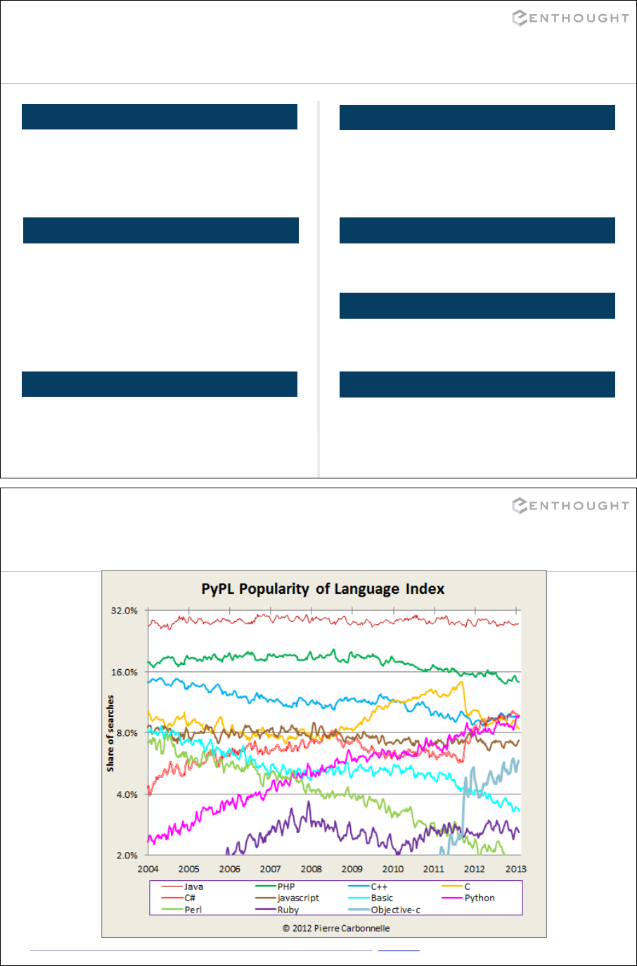
PYPL PopularitY of Programming Language index
* https://sites.google.com/site/pydatalog/pypl/PyPL-PopularitY-of-Programming-Language (CC by 3.0 license)
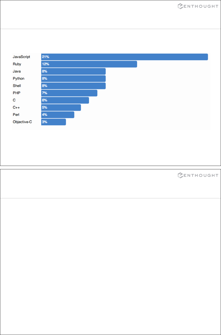
GitHub Top Languages 2013
5
6
IPython
An enhanced
interactive Python shell
7
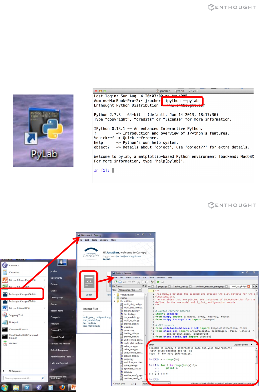
Starting IPython
IPython can be started:
•by typing ipython --pylab in any
terminal/command prompt
•w/ the pylab icon
8
Starting IPython in Canopy
9
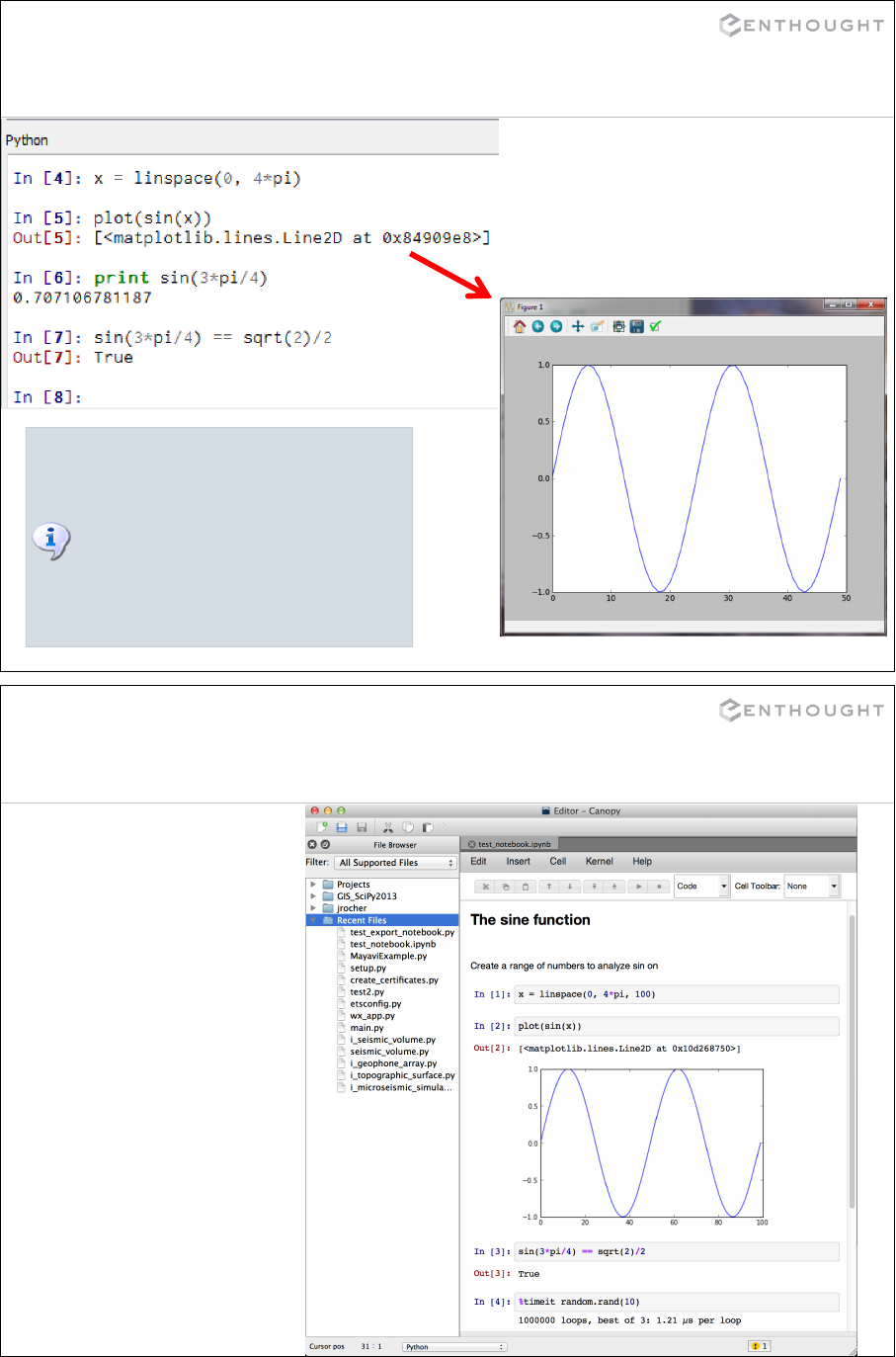
PyLab: Interactive Python Environment
The PyLab mode in IPython handles some
gory details behind the scenes. It allows
both the Python command interpreter
(above) and the GUI plot window (right) to
coexist. This involves a bit of multi-
threaded magic.
PyLab also imports some handy functions
into the command interpreter for user
convenience.
10
IPython notebook: exportable session
Contains in 1 file the
inputs, the outputs,
figures, plain text
(markdown), titles and
more...
•.ipynb files.
•Create a new one in
Canopy by selecting:
File > New >
IPython notebook

11
IPython
In [1]: a=1
In [2]: a
Out[2]: 1
STANDARD PYTHON
In [3]: b = [1,2,3]
# List available variables.
In [4]: %whos
Variable Type Data/Info
----------------------------
a int 1
b list n=3
# Remove user defined variables.
In [5]: %reset
In [6]: %whos
Interactive namespace is empty.
In [7]: plot
NameError: name 'plot' is not
defined
# Reload pylab.
In [8]: %pylab
Welcome to pylab,…
RESET
AVAILABLE VARIABLES “%reset” also removes the
names imported by PyLab,
such as the plot command.
12
# Change directory (note Unix style forward slashes!)
In [9]: cd c:/python_class/Demos/speed_of_light
c:\python_class\Demos\speed_of_light
# List directory contents (Unix style, not “dir”).
In [10]: ls
Volume in drive C has no label.
Volume Serial Number is 5417-593D
Directory of c:\python_class\Demos\speed_of_light
09/01/2008 02:53 PM <DIR> .
09/01/2008 02:53 PM <DIR> ..
09/01/2008 02:48 PM 1,188 exercise_speed_of_light.txt
09/01/2008 02:48 PM 2,682,023 measurement_description.pdf
09/01/2008 02:48 PM 187,087 newcomb_experiment.pdf
09/01/2008 02:48 PM 1,312 speed_of_light.dat
09/01/2008 02:48 PM 1,436 speed_of_light.py
09/01/2008 02:48 PM 1,232 speed_of_light2.py
6 File(s) 2,874,278 bytes
2 Dir(s) 11,997,437,952 bytes free
Directory Navigation in IPython
Tab completion helps you find and type directory and file names.
13
# Print working directory name (Unix style, not “cd”).
In [11]: pwd
c:\python_class\Demos\speed_of_light
# Bookmark the demo and exercise directories, so we can return
# to them easily.
In [12]: cd ..
c:\python_class\Demos
In [13]: %bookmark demo
In [14]: cd ../Exercises
c:\python_class\Exercises
In [15]: %bookmark exer
In [16]: %bookmark –l
demo -> c:\python_class\Demos
exer -> c:\python_class\Exercises
In [17]: cd demo
(bookmark:demo) -> c:\python_class\Demos
Directory Bookmarks
14
# tab completion
In [11]: %run speed_of_li
speed_of_light.dat speed_of_light.py
# execute a python file
In [11]: %run speed_of_light.py
Running Scripts in IPython

15
Function Info
# Follow a command with '?' to print its documentation.
In [19]: len?
Type: builtin_function_or_method
Base Class: <type 'builtin_function_or_method'>
String Form: <built-in function len>
Namespace: Python builtin
Docstring:
len(object) -> integer
Return the number of items of a sequence or mapping.
HELP USING ?
16
Function Info
# Follow a command with '??' to print its source code.
In [43]: squeeze??
def squeeze(a):
"""Remove single-dimensional entries from the shape of a.
Examples
--------
>>> x = array([[[1,1,1],[2,2,2],[3,3,3]]])
>>> x.shape
(1, 3, 3)
>>> squeeze(x).shape
(3, 3)
"""
try:
squeeze = a.squeeze
except AttributeError:
return _wrapit(a, 'squeeze')
return squeeze()
?? can’t show the source
code for “extension” functions
that are implemented in C.
SHOW SOURCE CODE USING ??

17
IPython History
HISTORY COMMAND
# list previous commands. Use
# ‘magic’ % because ‘hist’ is
# histogram function in pylab
In [3]: %hist
a=1
a
# list string from prompt[2]
In [4]: _i2
Out[4]: 'a\n'
INPUT HISTORY
# grab previous result
In [5]: _
Out[5]: 'a\n’
# grab result from prompt[2]
In [6]: _2
Out[6]: 1
OUTPUT HISTORY
The up and down arrows
scroll through your ipython
input history.
18
Reading Simple Tracebacks
In [9]: 1 + "hello"
--------------------
TypeError Traceback (most recent call last)
C:\...<ipython-input…> in <module>()
----> 1 1 + "hello"
TypeError: unsupported operand type(s) for +: 'int' and 'str'
ERROR ADDING AN INTEGER TO A STRING
The “type” of error
that occurred. Short message about
why it occurred.
Location and code
where error occurred.
# Again we fail when adding two variables, but note that the
# traceback tells us we have a completely different problem.
# In this case, our variable doesn't exist, so the operation fails.
In [10]: undefined_var + 1
…
NameError: name 'undefined_var' is not defined
ERROR TRYING TO ADD A NON-EXISTENT VARIABLE

19
Language Introduction
20
# real numbers
>>> b = 1.4 + 2.3
>>> b
3.6999999999999997
# "prettier" version.
>>> print b
3.7
>>> type(b)
<type 'float'>
# complex numbers
>>> c = 2+1.5j
>>> c
(2+1.5j)
# adding two values
>>> 1 + 1
2
# setting a variable
>>> a = 1
>>> a
1
# checking a variable’s type
>>> type(a)
<type 'int'>
# an arbitrarily long integer
>>> a = 12345678901234567890
>>> a
12345678901234567890L
>>> type(a)
<type 'long'>
# Remove 'a' from the 'namespace'
>>> del a
>>> a
NameError: name 'a' is not
defined
Interactive Calculator
The four numeric types in Python on 32-bit
architectures are:
integer (4 byte)
long integer (any precision)
float (8 byte like C’s double)
complex (16 byte)
The numpy module, which we will see later,
supports a larger number of numeric types.

21
# don't do this
>>> max = 100
# ...some time later...
>>> x = max(4, 5)
TypeError: 'int' object is not
callable
>>> 1+2-(3*4/6)**5+(7%5)
-27
More Interactive Calculation
ARITHMETIC OPERATIONS
>>> abs(-3)
3
>>> max(0, min(10, -1, 4, 3))
0
>>> round(2.718281828)
3.0
SIMPLE MATH FUNCTIONS
TYPE CONVERSION
>>> int(2.718281828)
2
>>> float(2)
2.0
>>> 1+2.0
3.0
OVERWRITING FUNCTIONS (!)
ALTERNATIVE NOTATIONS
>>> 0xFF
255
>>> 023 # octal!
19
>>> 6e3
6000.0
IN-PLACE OPERATIONS
>>> b = 2.5
>>> b += 0.5 # b = b + 0.5
>>> b
3.0
# Also -=, *=, /=, etc.
22
>>> q = 1 > 0
>>> q
True
>>> type(q)
<type 'bool'>
# <, >, <=, >=, ==, !=
>>> 1 >= 2
False
>>> 1 + 1 == 2
True
>>> 2**3 != 3**2
True
# Chained comparisons
>>> 1 < 10 < 100
True
Logical expressions, bool data type
COMPARISON OPERATORS
bool DATA TYPE
and OPERATOR
>>> 1 > 0 and 5 == 5
True
# If first operand is false,
# the second is not evaluated.
>>> 1 < 0 and max(0,1,2) > 1
False
>>> a = 50
>>> a < 10 or a > 90
False
# If first operand is true,
# the second is not evaluated.
>>> a = 0
>>> a < 10 or a > 90
True
or OPERATOR
>>> not 10 <= a <= 90
True
not OPERATOR

23
Strings
# using double quotes
>>> s = "hello world"
>>> print s
hello world
# single quotes also work
>>> s = 'hello world'
>>> print s
hello world
>>> s = "12345"
>>> len(s)
5
CREATING STRINGS
# concatenating two strings
>>> "hello " + "world"
'hello world'
# repeating a string
>>> "hello " * 3
'hello hello hello '
STRING OPERATIONS
STRING LENGTH
SPLIT/JOIN STRINGS
# split space-delimited words
>>> s = "hello world"
>>> wrd_lst = s.split()
>>> print wrd_lst
['hello', 'world']
# join words back together
# with a space in between
>>> space = ' '
>>> space.join(wrd_lst)
'hello world'
24
A few string methods and functions
>>> s = "hello world"
>>> s.replace('world','Mars')
'hello Mars'
REPLACING TEXT
CONVERT TO UPPER CASE
>>> s.upper()
'HELLO WORLD'
>>> s = "\t hello \n"
>>> s.strip()
'hello'
REMOVE WHITESPACE
NUMBERS TO STRINGS
>>> str(1.1 + 2.2)
'3.3'
>>> repr(1.1 + 2.2)
'3.3000000000000003'
>>> str(1)
'1'
>>> hex(255)
'0xFF'
>>> oct(19)
'023'
STRINGS TO NUMBERS
>>> int('23')
23
>>> int('FF', 16)
255
>>> float('23')
23.0

25
Available string methods
# list available methods on a string
>>> dir(s)
[…
'capitalize',
'center',
'count',
'decode',
'encode',
'endswith',
'expandtabs',
'find',
'format',
'index',
'isalnum',
'isalpha',
'isdigit',
'islower',
'isspace',
'istitle',
'isupper',
'join',
'ljust',
'lower',
'lstrip',
'partition',
'replace',
'rfind',
'rindex',
'rjust',
'rpartition',
'rsplit',
'rstrip',
'split',
'splitlines',
'startswith',
'strip',
'swapcase',
'title',
'translate',
'upper',
'zfill']
26
Multi-line Strings
# strings in triple quotes
# retain line breaks
>>> a = """hello
... world"""
>>> print a
hello
world
# The \ character means line
# continuation. Be careful
# because it must be the last
# character on line.
>>> a = "hello " \
... "world"
>>> print a
hello world
TRIPLE QUOTES
# group strings using
# parentheses
>>> a = ("hello "
... "world")
>>> print a
hello world
MULTI-LINE WITH PARENTHESES
LINE CONTINUATION
# including the new line
>>> a = "hello\nworld"
>>> print a
hello
world
NEW LINE CHARACTER

String Formatting
str.format(*args, **kwargs)
Replacement field: {<field_name> :<format_spec> }
•Delimited by curly brackets. (Use {{ and }} to include curly brackets in the output.)
•If field_name is an integer, it refers to a position in the positional arguments:
>>> '{0} is greater than {1}'.format(100, 50)
'100 is greater than 50'
•If field_name is a name, it refers to a keyword argument:
>>> '{last}, {first}'.format(first='Ellen', last='Ripley')
'Ripley, Ellen'
The format() method replaces the replacement fields in the string with the values given as
arguments. Any other text in the string remains unchanged. For example:
Optional
>>> '{0:2d}-{1}: {name}, ${price:.2f}'.format(7, 19, name='SC1', price=3.4)
' 7-19: SC1, $3.40'
27
28
String Formatting - Format Spec
ALIGNMENT OPTION
Type Meaning
b Binary format.
c Character; converts int to unicode char.
d Decimal integer (base 10).
o Octal (base 8).
x Hex (base 16), lower case.
X Hex (base 16), upper case.
n Number; same as 'd', but uses current locale.
None Same as 'd'.
INTEGER TYPE CODES
For numbers only.
Char Meaning
+ Include a sign for positive and negative number.
- Indicate sign for negative numbers only (default)
space Include a leading space for positive numbers.
SIGN OPTION
FLOATING POINT TYPE CODES
Type Meaning
e Scientific notation.
E Scientific notation, with upper case 'E'.
f Fixed point.
F Fixed point; same as 'f'.
g General format.
G General format; same as 'g', with upper case 'E' when
necessary.
n Number; same as 'g', but uses current locale.
% Percentage. Multiplies by 100 and displays with 'f',
followed by a percent sign.
None Same as 'g'.
STRING TYPE CODES
Type Meaning
s String. This is the default, and may be omitted.
Char Meaning
< Left aligned.
> Right aligned.
= (For numeric types only.) Pad after the sign but
before the digits (e.g. +000000120).
^ Center within the available space.
If an alignment character is given, it may be preceded by
a fill character.
The format spec is a sequence of characters
including:
•the alignment option,
•the sign option,
•the width (and .precision) option
•the type code.
>>> 'price: ${0:=-7.2f}'.format(3.4)
'price: $ 3.40'

29
String Formatting - Examples
# Basic string formatting
>>> print '{} {} {}'.format('a', 'b', 'c')
a b c
# Numbered fields refer to the position of the arguments
>>> print '{2} {1} {0}'.format('a', 'b', 'c')
c b a
# Named fields refer to keyword arguments
>>> print '{color} {n} {x}'.format(n=10, x=1.5, color='blue')
blue 10 1.5
# Positional and keyword arguments can be combined
>>> print '{color} {0} {x} {1}'.format(10, 'foo', x=1.5, color='blue')
blue 10 1.5 foo
# Precision and padding
>>> from math import pi
>>> print '{0:10} {1:10d} {c:10.2f}'.format('foo', 5, c=2*pi)
foo 5 6.28
30
String Formatting - Examples cont.
# Fixed point format (and a named keyword argument).
>>> print '[{x:5.0f}] [{x:5.1f}] [{x:5.2f}]'.format(x=12.3456)
[ 12] [ 12.3] [12.35]
# Sign options.
>>> '{:-f}; {:-f}'.format(3.14, -3.14) # Default
'3.140000; -3.140000'
>>> '{:+f}; {:+f}'.format(3.14, -3.14) # Use '+'
'+3.140000; -3.140000'
>>> '{: f}; {: f}'.format(3.14, -3.14) # Use ' '
' 3.140000; -3.140000'
# Alignment (and using a numbered positional argument).
>>> print '[{0:<10s}] [{0:>10s}] [{0:^10s}]'.format('PYTHON')
[PYTHON ] [ PYTHON] [ PYTHON ]
# Alignment with fill character.
>>> print '[{0:*<10s}] [{0:*>10s}] [{0:*^10s}]'.format('PYTHON')
[PYTHON****] [****PYTHON] [**PYTHON**]
# Different bases for an integer (hex, decimal, octal, binary).
>>> '{0:X} {0:d} {0:o} {0:b}'.format(254)
'FE 254 376 11111110'

31
Formatting with %
FORMAT OPERATOR %
# the % operator formats values
# to strings using C conventions.
>>> s = "some numbers:"
>>> x = 1.34
>>> y = 2
>>> t = "%s %f, %d" % (s,x,y)
>>> print t
some numbers: 1.340000, 2
>>> y = -2.1
>>> print "%f\n%f" % (x,y)
1.340000
-2.100000
>>> print "% f\n% f" % (x,y)
1.340000
-2.100000
>>> print "%4.2f" % x
1.34
Conversion Meaning
d or i Signed integer decimal
o Unsigned octal
u Unsigned decimal
x Unsigned hexadecimal (lowercase)
X Unsigned hexadecimal (uppercase)
e Floating point exponential format (lowercase)
E Floating point exponential format (uppercase)
F or f Floating point decimal format
G or g Floating point format or exponential
c Single character
r Converts object using repr()
s Converts object using str()
CONVERSION CODES
Flag Meaning
0 The conversion will be zero padded for
numeric values.
- The converted value is left adjusted (overrides
the "0" conversion if both are given).
<space> (a space) A blank should be left before a
positive number (or empty string) produced by
a signed conversion.
+ A sign character ("+" or "-") will precede the
conversion (overrides a "space" flag).
CONVERSION FLAGS
32
List objects
>>> a = [10,11,12,13,14]
>>> print a
[10, 11, 12, 13, 14]
LIST CREATION WITH BRACKETS
# simply use the + operator
>>> [10, 11] + [12, 13]
[10, 11, 12, 13]
CONCATENATING LIST
REPEATING ELEMENTS IN LISTS
# the range function is helpful
# for creating a sequence
>>> range(5)
[0, 1, 2, 3, 4]
>>> range(2,7)
[2, 3, 4, 5, 6]
>>> range(2,7,2)
[2, 4, 6]
# the multiply operator
# does the trick
>>> [10, 11] * 3
[10, 11, 10, 11, 10, 11]
range(start, stop, step)

33
Indexing
# list
# indices: 0 1 2 3 4
>>> a = [10,11,12,13,14]
>>> a[0]
10
RETRIEVING AN ELEMENT
The first element in an array has index=0
as in C. Take note Fortran programmers!
NEGATIVE INDICES
# negative indices count
# backward from the end of
# the list
#
# indices: -5 -4 -3 -2 -1
>>> a = [10,11,12,13,14]
>>> a[-1]
14
>>> a[-2]
13
SETTING AN ELEMENT
>>> a[1] = 21
>>> print a
[10, 21, 12, 13, 14]
OUT OF BOUNDS
>>> a[10]
Traceback (innermost last):
File "<interactive input>",line 1,in ?
IndexError: list index out of range
34
More on list objects
# use in or not in
>>> a = [10,11,12,13,14]
>>> 13 in a
True
>>> 13 not in a
False
DOES THE LIST CONTAIN x ?
LIST CONTAINING MULTIPLE
TYPES
# list containing integer,
# string, and another list
>>> a = [10,'eleven',[12,13]]
>>> a[1]
'eleven'
>>> a[2]
[12, 13]
# use multiple indices to
# retrieve elements from
# nested lists
>>> a[2][0]
12
>>> len(a)
3
LENGTH OF A LIST
# use the del keyword
>>> del a[2]
>>> a
[10,'eleven']
DELETING OBJECT FROM LIST
Prior to version 2.5, Python was limited to
sequences with ~2 billion elements.
Python 2.5 can handle up to 263 elements.

35
Slicing
# indices:
# -5 -4 -3 -2 -1
# 0 1 2 3 4
>>> a = [10,11,12,13,14]
# [10,11,12,13,14]
>>> a[1:3]
[11, 12]
# negative indices work also
>>> a[1:-2]
[11, 12]
>>> a[-4:3]
[11, 12]
SLICING LISTS
# omitted boundaries are
# assumed to be the beginning
# (or end) of the list
# grab first three elements
>>> a[:3]
[10, 11, 12]
# grab last two elements
>>> a[-2:]
[13, 14]
# every other element
>>> a[::2]
[10, 12, 14]
var[lower:upper:step]
Extracts a portion of a sequence by specifying a lower and upper bound.
The lower-bound element is included, but the upper-bound element is not included.
Mathematically: [lower, upper). The step value specifies the stride between elements.
OMITTING INDICES
36
A few methods for list objects
some_list.reverse( )
Add the element x to the end
of the list some_list.
some_list.sort( cmp )
some_list.append( x )
some_list.index( x )
some_list.count( x ) some_list.remove( x )
Count the number of times x
occurs in the list.
Return the index of the first
occurrence of x in the list.
Delete the first occurrence of x from the
list.
Reverse the order of elements in the
list.
By default, sort the elements in
ascending order. If a compare
function is given, use it to sort
the list.
some_list.extend( sequence )
Concatenate sequence onto this list.
some_list.insert( index, x )
Insert x before the specified index.
Return the element at the specified
index. Also, remove it from the list.
some_list.pop( index )

37
List methods in action
>>> a = [10,21,23,11,24]
# add an element to the list
>>> a.append(11)
>>> print a
[10,21,23,11,24,11]
# how many 11s are there?
>>> a.count(11)
2
# extend with another list
>>> a.extend([5,4])
>>> print a
[10,21,23,11,24,11,5,4]
# where does 11 first occur?
>>> a.index(11)
3
# insert 100 at index 2?
>>> a.insert(2, 100)
>>> print a
[10,21,100,23,11,24,11,5,4]
# pop the item at index=3
>>> a.pop(3)
23
# remove the first 11
>>> a.remove(11)
>>> print a
[10,21,100,24,11,5,4]
# sort the list (in-place)
# Note: use sorted(a) to
# return a new list.
>>> a.sort()
>>> print a
[4,5,10,11,21,24,100]
# reverse the list
>>> a.reverse()
>>> print a
[100,24,21,11,10,5,4]
38
Mutable vs. Immutable
# Mutable objects, such as
# lists, can be changed
# in place.
# insert new values into list
>>> a = [10,11,12,13,14]
>>> a[1:3] = [5,6]
>>> print a
[10, 5, 6, 13, 14]
MUTABLE OBJECTS IMMUTABLE OBJECTS
# Immutable objects, such as
# integers and strings,
# cannot be changed in place.
# try inserting values into
# a string
>>> s = 'abcde'
>>> s[1:3] = 'xy'
Traceback (innermost last):
File "<interactive input>",line 1,in ?
TypeError: object doesn't support
slice assignment
# here's how to do it
>>> s = s[:1] + 'xy' + s[3:]
>>> print s
'axyde'
The cStringIO module treats strings
like a file buffer and allows insertions.
It’s useful when working with large
strings or when speed is paramount.

39
Tuple – Immutable Sequence
>>> a = (10,11,12,13,14)
>>> print a
(10, 11, 12, 13, 14)
TUPLE CREATION
PARENTHESES ARE OPTIONAL
LENGTH-1 TUPLE
>>> (10,)
(10,)
>>> (10)
10
TUPLES ARE IMMUTABLE
>>> a = 10,11,12,13,14
>>> print a
(10, 11, 12, 13, 14)
(10) is not a tuple,
but an integer
with parentheses.
# create a list
>>> a = range(10,15)
[10, 11, 12, 13, 14]
# cast the list to a tuple
>>> b = tuple(a)
>>> print b
(10, 11, 12, 13, 14)
# try inserting a value
>>> b[3] = 23
TypeError: 'tuple' object doesn't
support item assignment
40
Dictionaries
Dictionaries store key/value pairs. Indexing a dictionary by a key returns
the value associated with it. The key must be immutable.
# Create an empty dictionary using curly brackets.
>>> record = {}
# Each indexed assignment creates a new key/value pair.
>>> record['first'] = 'Jmes'
>>> record['last'] = 'Maxwell'
>>> record['born'] = 1831
>>> print record
{'first': 'Jmes', 'born': 1831, 'last': 'Maxwell'}
# Create another dictionary with initial entries.
>>> new_record = {'first': 'James', 'middle':'Clerk'}
# Now update the first dictionary with values from the new one.
>>> record.update(new_record)
>>> print record
{'first': 'James', 'middle': 'Clerk', 'last':'Maxwell', 'born':
1831}
DICTIONARY EXAMPLE

41
Accessing and deleting keys and values
ACCESS USING INDEX NOTATION REMOVE AN ENTRY WITH DEL
ACCESS WITH get(key, default)
>>> print record['first']
James
>>> del record['middle']
>>> record
{'born': 1831, 'first':
'James', 'last': 'Maxwell'}
The get() method returns the value
associated with a key; the optional
second argument is the return value if
the key is not in the dictionary.
>>> record.get('born',0)
1831
>>> record.get('home', 'TBD')
'TBD'
>>> record['home']
KeyError: ...
REMOVE WITH pop(key, default)
pop() removes the key from the
dictionary and returns the value; the
optional second argument is the return
value if the key is not in the dictionary.
>>> record.pop('born', 0)
1831
>>> record
{'first': 'James', 'last':
'Maxwell'}
>>> record.pop('born', 0)
0
42
A few dictionary methods
some_dict.clear( )
some_dict.copy( )
x in some_dict
some_dict.keys( )
some_dict.values( )
some_dict.items( )
Remove all key/value pairs from
the dictionary, some_dict.
Create a copy of the dictionary
Test whether the dictionary contains the
key x.
Return a list of all the keys in the
dictionary.
Return a list of all the values in the
dictionary.
Return a list of all the key/value pairs in
the dictionary.

43
Dictionary methods in action
# dict of animals:count pairs
>>> barn = {'cows': 1,
... 'dogs': 5,
... 'cats': 3}
# test for chickens
>>> 'chickens' in barn
False
# get a list of all keys
>>> barn.keys()
['cats','dogs','cows']
# get a list of all values
>>> barn.values()
[3, 5, 1]
# return key/value tuples
>>> barn.items()
[('cats', 3), ('dogs', 5),
('cows', 1)]
# How many cats?
>>> barn['cats']
3
# Change the number of cats.
>>> barn['cats'] = 10
>>> barn['cats']
10
# Add some sheep.
>>> barn['sheep'] = 5
>>> barn['sheep']
5
44
Set objects
A set is an unordered collection of
unique, immutable objects.
DEFINITION
# an empty set
>>> s = set()
# convert a sequence to set
>>> t = set([1,2,3,1])
# note removal of duplicates
>>> t
set([1, 2, 3])
CONSTRUCTION
ADD ELEMENTS
# Remove an element. Raise
# exception if not in the set.
>>> t.remove(1)
>>> t
set([2, 3, 5, 6, 7])
# Remove and return an
# arbitrary element from the set.
>>> t.pop()
2
# Remove element from list
# if it exists.
>>> t.discard(3)
>>> t
set([5, 6, 7])
# Otherwise, do nothing.
>>> t.discard(20)
>>> t
set([5, 6, 7])
>>> t.add(5)
set([1, 2, 3, 5])
>>> t.update([5,6,7])
set([1, 2, 3, 5, 6, 7])
REMOVE ELEMENTS

45
Set Operations
A B
A B
A B
>>> a.union(b)
set([1, 2, 3, 4, 5, 6])
>>> a | b
set([1, 2, 3, 4, 5, 6])
UNION
INTERSECTION
>>> a.symmetric_difference(b)
set([1, 2, 5, 6])
>>> a ^ b #xor
set([1, 2, 5, 6])
>>> a.intersection(b)
set([3, 4])
>>> a & b
set([3, 4])
SYMMETRIC DIFFERENCE
>>> a.difference(b)
set([1, 2])
>>> a – b
set([1, 2])
DIFFERENCE
>>> a = set([1,2,3,4])
>>> b = set([3,4,5,6])
OVERLAPPING SETS
A B
A B
46
Set Containment
AB
# Is b fully contained in a?
>>> b.issubset(a)
True
>>> b <= a
True
ISSUBSET ISSUPERSET
>>> a = set([1,2,3])
>>> b = set([1,2])
OVERLAPPING SETS
# Does a fully contain b?
>>> a.issuperset(b)
True
>>> a >= b
True
There is also an immutable type of
set called a frozenset (analogous to
a tuple) which can be used as a
dictionary key or an element of a
set.
47
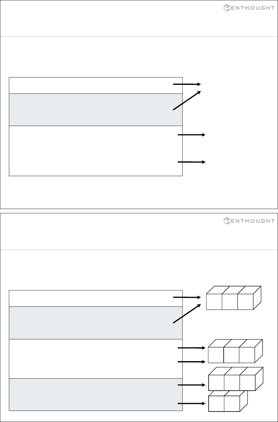
Assignment of “simple” object
>>> x = 0
Assignment creates object references.
x
y
# This causes x and y to point
# to the same value.
>>> y = x
# Re-assigning y to a new value
# decouples the two variables.
>>> y = "foo"
>>> print x
0
x
y
0
0
foo
48
3 4
Assignment of Container object
>>> x = [0, 1, 2]
Assignment creates object references.
0 1 2
x
y
# This causes x and y to point
# to the same list.
>>> y = x
# A change to y also changes x.
>>> y[1] = 6
>>> print x
[0, 6, 2]
0 6 2
x
y
# Re-assigning y to a new list
# decouples the two variables.
>>> y = [3, 4]
x
0 6 2
y

49
If statements
if/elif/else provides conditional execution of code blocks.
if <condition>:
<statement 1>
<statement 2>
elif <condition>:
<statements>
else:
<statements>
# a simple if statement
>>> x = 10
>>> if x > 0:
... print 'Hey!'
... print 'x > 0'
... elif x == 0:
... print 'x is 0'
... else:
... print 'x is negative'
... < hit return >
Hey!
x > 0
IF EXAMPLE IF STATEMENT FORMAT
50
Test Values
•zero, None, “”, and empty objects are treated as False.
•All other objects are treated as True.
# empty objects test as false
>>> x = []
>>> if x:
... print 1
... else:
... print 0
... < hit return >
0
EMPTY OBJECTS
It often pays to be explicit. If you are
testing for an empty list, then test for:
if len(x) == 0:
...
This is clearer to future readers of
your code. It also can avoid bugs
where x==None may be passed in and
unexpectedly go down this path.

51
While loops
while loops iterate until a condition is met
# the condition tested is
# whether lst is empty
>>> lst = range(3)
>>> while lst:
... print lst
... lst = lst[1:]
... < hit return >
[0, 1, 2]
[1, 2]
[2]
while <condition>:
<statements>
WHILE LOOP BREAKING OUT OF A LOOP
# breaking from an infinite
# loop
>>> i = 0
>>> while True:
... if i < 3:
... print i,
... else:
... break
... i = i + 1
... < hit return >
0 1 2
52
For loops
for loops iterate over a sequence of objects
>>> for item in range(5):
... print item,
... < hit return >
0 1 2 3 4
# For a large range, xrange()
# is faster and more memory
# efficient.
>>> for item in xrange(10**6):
... print item,
... < hit return >
0 1 2 3 4 5 6 7 8 9 10 11 ...
>>> animals=['dogs','cats',
... 'bears']
>>> accum = ''
>>> for animal in animals:
... accum += animal + ' '
... < hit return >
>>> print accum
dogs cats bears
for <loop_var> in <sequence>:
<statements>
TYPICAL SCENARIO LOOPING OVER A STRING
>>> for item in 'abcde':
... print item,
... < hit return >
a b c d e
LOOPING OVER A LIST

53
List Comprehension
# element by element transform of
# a list by applying an
# expression to each element
>>> a = [10,21,23,11,24]
>>> results=[]
>>> for val in a:
... results.append(val+1)
>>> results
[11, 22, 24, 12, 25]
LIST TRANSFORM WITH LOOP LIST COMPREHENSION
# list comprehensions provide
# a concise syntax for this sort
# of element by element
# transformation
>>> a = [10,21,23,11,24]
>>> [val+1 for val in a]
[11, 22, 24, 12, 25]
LIST COMPREHENSION WITH
FILTER
>>> a = [10,21,23,11,24]
>>> [val+1 for val in a if val>15]
[22, 24, 25]
# transform only elements that
# meet a criteria
>>> a = [10,21,23,11,24]
>>> results=[]
>>> for val in a:
... if val>15:
... results.append(val+1)
>>> results
[22, 24, 25]
FILTER-TRANSFORM WITH LOOP
Consider using a list
comprehension whenever you
need to transform one sequence
to another.
54
Generator Expressions
>>> set([str(i) for i in range(5)])
set(['1', '0', '3', '2', '4'])
# tests on sequences
>>> any([i >= 3 for i in range(5)])
True
>>> all([i >= 3 for i in range(5)])
False
# summation
>>> sum([i**2 for i in range(5)])
30
LIST COMPREHENSION
>>> set(str(i) for i in range(5))
set(['1', '0', '3', '2', '4'])
# tests on sequences
>>> any(i >= 3 for i in range(5))
True
>>> all(i >= 3 for i in range(5))
False
# summation
>>> sum(i**2 for i in range(5))
30
Generator expressions are like list comprehensions without the brackets:
GENERATOR EXPRESSION

55
Multiple assignments
# creating a tuple without ()
>>> d = 1,2,3
>>> d
(1, 2, 3)
# multiple assignments
>>> a,b,c = 1,2,3
>>> print b
2
# multiple assignments from a
# tuple
>>> a,b,c = d
>>> print b
2
# also works for lists
>>> a,b,c = [1,2,3]
>>> print b
2
FROM TUPLE TO TUPLE FROM LIST TO TUPLE
56
Looping Patterns
# Looping through a sequence of
# tuples allows multiple
# variables to be assigned.
>>> pairs = [(0,'a'),(1,'b'),
... (2,'c')]
>>> for index, value in pairs:
... print index, value
0 a
1 b
2 c
MULTIPLE LOOP VARIABLES ZIP
# zip 2 or more sequences
# into a list of tuples
>>> x = [0, 1, 2]
>>> y = ['a', 'b', 'c']
>>> zip(x,y)
[(0,'a'), (1,'b'), (2,'c')]
>>> for index, value in zip(x,y):
... print index, value
0 a
1 b
2 c
ENUMERATE
# enumerate -> index, item.
>>> y = ['a', 'b', 'c']
>>> for index, value in enumerate(y):
... print index, value
0 a
1 b
2 c
REVERSED
>>> z = [(0,'a'),(1,'b'),(2,'c')]
for index, value in reversed(z):
... print index, value
2 c
1 b
0 a

57
Looping over a dictionary
>>> for key in d:
... print key, d[key]
a 1
c 3
b 2
DEFAULT LOOPING (KEYS)
LOOPING OVER KEYS (EXPLICIT)
>>> for key in d.keys():
... print key, d[key]
a 1
c 3
b 2
>>> d = {'a':1, 'b':2, 'c':3}
>>> for val in d.values():
... print val
1
3
2
LOOPING OVER VALUES
LOOPING OVER ITEMS
>>> for key, val in d.items():
... print key, val
a 1
c 3
b 2
59
Anatomy of a function
def add(arg0, arg1):
"""Add two numbers"""
a = arg0 + arg1
return a
Function arguments are listed,
separated by commas. They are passed
by assignment.
The keyword def indicates the
start of a function.
Indentation is
used to indicate
the contents of
the function. It
is not optional,
but a part of the
syntax.
An optional return
statement specifies
the value returned from the
function. If return is omitted,
the function returns the
special value None.
A colon ( : )
terminates
the function
signature.
An optional docstring
documents the function
in a standard way for
tools like ipython.

60
Our new function in action
# We'll create our function
# on the fly in the
# interpreter.
>>> def add(x,y):
... a = x + y
... return a
# Test it out with numbers.
>>> val_1 = 2
>>> val_2 = 3
>>> add(val_1,val_2)
5
# How about strings?
>>> val_1 = 'foo'
>>> val_2 = 'bar'
>>> add(val_1,val_2)
'foobar'
# Functions can be assigned
# to variables.
>>> func = add
>>> func(val_1, val_2)
'foobar'
# How about numbers and strings?
>>> add('abc',1)
Traceback (innermost last):
File "<interactive input>", line 1, in ?
File "<interactive input>", line 2, in add
TypeError: cannot add type "int" to string
61
Function Calling Conventions
# The "standard" calling
# convention we know and love.
>>> def add(x, y):
... return x + y
>>> add(2, 3)
5
POSITIONAL ARGUMENTS DEFAULT VALUES
# Arguments can be
# assigned default values.
>>> def quad(x,a=1,b=1,c=0):
... return a*x**2 + b*x + c
# Use defaults for a, b and c.
>>> quad(2.0)
6.0
# Set b=3. Defaults for a & c.
>>> quad(2.0, b=3)
10.0
# Keyword arguments can be
# passed in out of order.
>>> quad(2.0, c=1, a=3, b=2)
17.0
# specify argument names
>>> add(x=2, y=3)
5
# or even a mixture if you are
# careful with order
>>> add(2, y=3)
5
KEYWORD ARGUMENTS

62
Function Calling Conventions
# Pass in any number of
# arguments. Extra arguments
# are put in the tuple args.
>>> def foo(x, y, *args):
... print x, y, args
>>> foo(2, 3, 'hello', 4)
2 3 ('hello', 4)
VARIABLE NUMBER OF ARGS VARIABLE KEYWORD ARGS
# Extra keyword arguments
# are put into the dict kw.
>>> def bar(x, y=1, **kw):
... print x, y, kw
>>> bar(1, y=2, a=1, b=2)
1 2 {'a': 1, 'b': 2}
63
Function Calling Conventions
# This signature takes any
# number of positional and
# keyword arguments.
>>> def foo(*args, **kw):
... print args, kw
>>> foo(2, 3, x='hello', y=4)
(2, 3) {'x': 'hello', 'y': 4}
THE ‘ANYTHING’ SIGNATURE
# To return multiple values
# from a function, we return
# a tuple containing those
# values. This is a common
# use of multiple (tuple)
# assignment.
>>> def functions(x):
... y1 = x**2 + x
... y2 = x**3 + x**2 + 2*x
... return y1, y2
>>> a, b = functions(c)
MULTIPLE FUNCTION RETURNS

64
Expanding Function Arguments
>>> def add(x, y):
... return x + y
# '*' in a function call
# converts a sequence into the
# arguments to a function.
>>> vars = [1,2]
>>> add(*vars)
3
POSITIONAL ARGUMENT
EXPANSION KEYWORD ARGUMENT
EXPANSION
>>> def bar(x, y=1, **kw):
... print x, y, kw
# '**' expands a
# dictionary into keyword
# arguments for a function.
vars = {'y':3, 'z':4}
>>> bar(1, **vars)
1, 3, {'z': 4}
65
Modules
# ex1.py
PI = 3.1416
def sum(lst):
tot = lst[0]
for value in lst[1:]:
tot = tot + value
return tot
w = [0,1,2,3]
print sum(w), PI
EX1.PY FROM SHELL
[ej@bull ej]$ python ex1.py
6 3.1416
FROM INTERPRETER
# load and execute the module
>>> import ex1
6 3.1416
# get/set a module variable
>>> print ex1.PI
3.1416
>>> ex1.PI = 3.14159
>>> print ex1.PI
3.14159
# call a module function
>>> t = [2,3,4]
>>> ex1.sum(t)
9

66
Modules cont.
# ex1.py version 2
PI = 3.14159
def sum(lst):
tot = 0
for value in lst:
tot = tot + value
return tot
w = [0,1,2,3,4]
print sum(w), PI
EDITED EX1.PY
INTERPRETER
# load and execute the module
>>> import ex1
6 3.1416
< edit file >
# import module again
>>> import ex1
# nothing happens!!!
# Use reload to force a
# previously imported library
# to be reloaded.
>>> reload(ex1)
10 3.14159
67
Modules cont. 2
A Python file can be used as a script, or as a module, or both.
# An example module that can
# be run as a script.
PI = 3.1416
def sum(lst):
""" Sum the values in a
list.
"""
tot = 0
for value in lst:
tot = tot + value
return tot
EX2.PY
def add(x,y):
" Add two values."
a = x + y
return a
def test():
w = [0,1,2,3]
assert( sum(w) == 6)
print 'test passed'
# This code runs only if this
# module is the main program.
if __name__ == '__main__':
test()

68
import Variations
# The most basic import
>>> import ex2
>>> ex2.PI
3.1416
BASIC IMPORTS
ALIASING A NAME
IMPORTING SPECIFIC SYMBOLS
IMPORTING *EVERYTHING*
# Pull *everything* into the
# local namespace.
>>> from ex2 import *
>>> PI
3.1416
>>> add(3,4.5)
7.5
# Use an ‘alias’
>>> import ex2 as e2
>>> e2.PI
3.1416
# Select specific names to
# bring into the local
# namespace.
>>> from ex2 import add, PI
>>> PI
3.1416
>>> add(2,3)
5
69
Modules cont. 3
foo/
__init__.py
bar.py (defines func)
baz.py (defines zap)
FILE STRUCTURE PACKAGES
Often a library will contain several
modules. These may be organized
in a hierarchical directory structure,
and imported using "dotted module
names". The first and the intermediate
names (if any) are called "packages".
Example:
>>> from foo.bar import func
>>> from foo.baz import zap
bar.py and baz.py are modules in the
package foo.
•The directory foo must be in the
python search path
•The file __init__.py indicates
that foo is a package. It may be an
empty file.
•In the simplest case:
package = directory
module = python file

70
Standard Modules
Python has a large library of standard modules ("batteries included"):
re - regular expressions
copy – shallow and deep copy operations
datetime - time and date objects
math, cmath - real and complex math
decimal, fractions - arbitrary precision
decimal and rational number objects
os, os.path, shutil - filesystem operations
sqlite3 - internal SQLite database
gzip, bz2, zipfile, tarfile – compression and
archiving formats
csv, netrc – file format handling
xml – various modules for handling XML
htmllib – an HTML parser
httplib, ftplib, poplib, socket, etc. –
modules for standard internet protocols
cmd – support for command interpreters
pdb – Python interactive debugger
profile, cProfile, timeit – Python profilers
collections, heapq, bisect – standard CS
algorithms and data structures
mmap – memory-mapped files
threading, Queue – threading support
multiprocessing – process based ‘threading’
subprocess – executing external commands
pickle, cPickle – object serialization
struct – interpret bytes as packed binary data
and many more… To see the content of one:
>>> dir(module_name)
71
Setting up PYTHONPATH
WINDOWS UNIX: .cshrc
UNIX: .bashrc
• Right-click on My Computer
• Click Properties
• Click Advanced Tab
• Click Environment Variables Button at
the bottom of the Advanced Tab
• Click New to create
PYTHONPATH or
• Click Edit to change existing
PYTHONPATH
• Changes take effect in the next
Command Prompt or IPython session.
PYTHONPATH is an environment variable (or set of registry entries on
Windows) that lists the directories Python searches for modules.
!! NOTE: The following should !!
!! all be on one line !!
setenv PYTHONPATH
$PYTHONPATH:$HOME/your_modules
PYTHONPATH=$PYTHONPATH:$HOME/your
_modules
export PYTHONPATH

72
Reading files
>>> results = []
>>> f = open('c:\\rcs.txt','r')
# Read all the lines.
>>> lines = f.readlines()
>>> f.close()
# Discard the header.
>>> lines = lines[1:]
>>> for line in lines:
... # split line into fields
... fields = line.split()
... # convert text to numbers
... freq = float(fields[0])
... vv = float(fields[1])
... hh = float(fields[2])
... # group & append to results
... all = [freq,vv,hh]
... results.append(all)
... < hit return >
FILE INPUT EXAMPLE
EXAMPLE FILE: RCS.TXT
#freq (MHz) vv (dB) hh (dB)
100 -20.3 -31.2
200 -22.7 -33.6
>>> for i in results: print i
[100.0, -20.30…, -31.20…]
[200.0, -22.70…, -33.60…]
PRINTING THE RESULTS
See demo/reading_files directory
for code.
73
More compact version
>>> results = []
>>> f = open('c:\\rcs.txt','r')
>>> f.readline()
'#freq (MHz) vv (dB) hh (dB)\n'
>>> for line in f:
... all = [float(val) for val in line.split()]
... results.append(all)
... < hit return >
>>> for i in results:
... print i
... < hit return >
ITERATING ON A FILE AND LIST COMPREHENSIONS
EXAMPLE FILE: RCS.TXT
#freq (MHz) vv (dB) hh (dB)
100 -20.3 -31.2
200 -22.7 -33.6

74
Writing files
>>> # Mode 'w': create new file:
>>> f = open('a.txt', 'w')
>>> f.write('Hello, world!')
>>> f.close()
>>> open('a.txt').read()
'Hello, world!'
>>> # Use the 'with' statement:
>>> with open('a.txt', 'w') as f:
.... f.write('Wow!')
....
>>> open('a.txt').read()
'Wow!'
>>> # Mode 'a': append to file:
>>> with open('a.txt', 'a') as f:
.... f.write(' Boo.')
....
>>> open('a.txt').read()
'Wow! Boo.'
FILE OUTPUT
>>> # Redirect output of a
>>> # print statement:
>>> f = open('a.txt', 'w')
>>> print >> f, "Here I am."
>>> f.close()
>>> open('a.txt').read()
'Here I am.\n'
REDIRECTED PRINT
WRITE AND READ
>>> f = open('a.txt', 'w+')
>>> print >> f, 12, 34, 56
>>> f.seek(3)
>>> f.read(2)
'34'
>>> f.close()
75
Particle Class Example
>>> class Particle(object):
... # Initializer method
... def __init__(self, m, v):
... self.mass = m # Assign attribute values of new object
... self.velocity = v
... # Method for calculating object momentum
... def momentum(self):
... return self.mass * self.velocity
... # A "magic" method defines object's string representation.
... # Evaluating the repr recovers the Particle object.
... def __repr__(self):
... return "Particle({0}, {1})".format(
... repr(self.mass), repr(self.velocity))
SIMPLE PARTICLE CLASS
EXAMPLE
>>> a = Particle(3.2, 4.1)
>>> print a.momentum()
13.12
>>> a
Particle(3.2, 4.1)

76
Overloading Addition
... def __add__(self, other)
... if not isinstance(other, Particle):
... return NotImplemented
... mnew = self.mass + other.mass
... vnew = (self.momentum() + other.momentum())/mnew
... return Particle(mnew, vnew)
SIMPLE PARTICLE CLASS
Classes can override many behaviors using special method names —
including numeric behavior.
EXAMPLE (cont.)
>>> b = Particle(8.6, 10.2)
>>> b, a
(Particle(8.6, 10.2), Particle(3.2, 4.1))
>>> c = a + b
>>> c
Particle(11.8, 8.545762711864406)
>>> print c.momentum()
100.84
77
Sorting
# sorting
>>> x = ['s','o','r','t']
# new list
>>> sorted(x)
['o', 'r', 's', 't']
# in-place
>>> x.sort()
>>> x
['o', 'r', 's', 't']
# reversing
# new list (note explicit 'list')
>>> x = ['b', 'a', 'c', 'k']
>>> list(reversed(x))
['k', 'c', 'a', 'b']
# in-place
>>> x.reverse()
>>> x
['k', 'c', 'a', 'b']
CUSTOM SORTS IN-PLACE VS NEW LIST
# define a key function to
# transform values before
# comparing in a sort
>>> def ignore_case(x):
... return x.lower()
>>> x = ['S','o','r','T']
>>> sorted(x)
['S', 'T', 'o', 'r']
>>> sorted(x, key=ignore_case)
['o', 'r', 'S', 'T']
78
Sorting
# comparison functions for a variety of particle values
>>> def by_mass(x):
... return x.mass
>>> def by_momentum(x):
... return x.momentum()
>>> def by_kinetic_energy(x):
... return 0.5*x.mass*x.velocity**2
# sorting particles in a list by their various properties
>>> from particle import Particle
>>> x = [Particle(1.2,3.4), Particle(2.1,2.3), Particle(4.6,.7)]
>>> sorted(x, key=by_mass)
[(m:1.2, v:3.4), (m:2.1, v:2.3), (m:4.6, v:0.7)]
>>> sorted(x, key=by_momentum)
[(m:4.6, v:0.7), (m:1.2, v:3.4), (m:2.1, v:2.3)]
>>> sorted(x, key=by_kinetic_energy)
[(m:4.6, v:0.7), (m:2.1, v:2.3), (m:1.2, v:3.4)]
SORTING CLASS INSTANCES
See demo/particle
directory for sample
code.
79
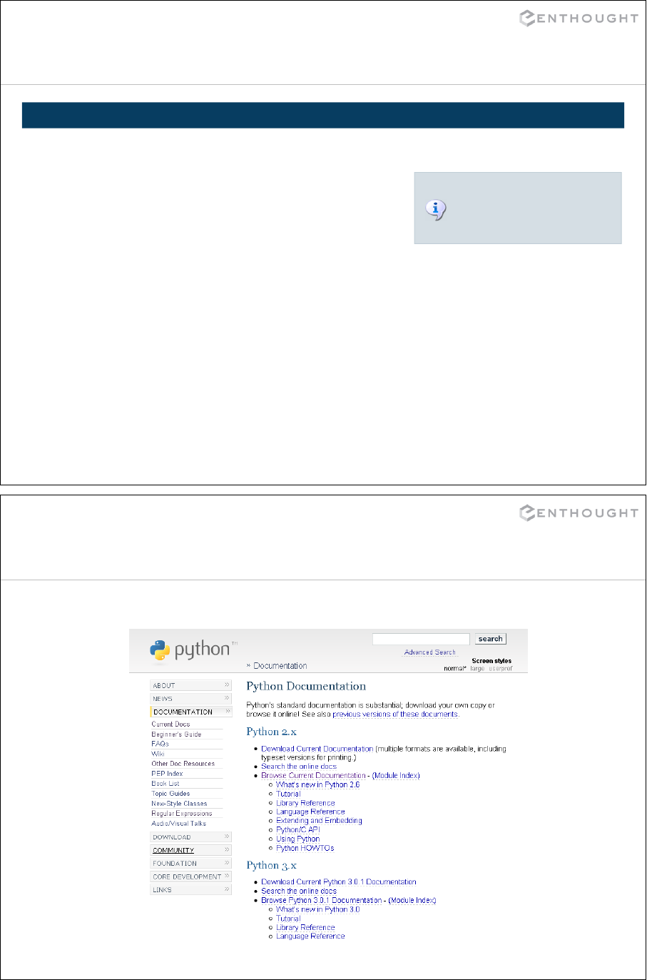
Excellent source of help
http://www.python.org/doc

80
Error and Exception
Handling
81
Basic Exception Handling
>>> import math
>>> math.log10(10.0)
1.0
>>> math.log10(0.0)
Traceback (innermost last):
ValueError: math domain error
>>> a = 0.0
>>> try:
... r = math.log10(a)
... except ValueError:
... print 'Warning: overflow occurred. Value set to -100.0'
... # set value to -100.0 and continue
... r = -100.0
Warning: overflow occurred. Value set to -100.0
>>> print r
-100.0
CATCHING ERROR AND CONTINUING
ERROR ON LOG OF ZERO

82
Exceptions
try:
a = value_bag[key]
r = math.log10(a)
except KeyError as error:
print "Variable '%s' not found" % error.args
ACCESS TO THE EXCEPTION OBJECT
try:
a = value_bag[key]
r = math.log10(a)
except KeyError as error:
print "Variable '%s' not found" % error.args
except ValueError:
print 'Warning: overflow occurred. Value set to -100.0'
# set value to -100.0 and continue
r = -100.0
MULTIPLE EXCEPTION CLAUSES
Exception Object
83
Exceptions
try:
a = value_bag[key]
r = math.log10(a)
except (KeyError, ValueError) as error:
print "an error occurred", error
HANDLING MULTIPLE EXCEPTIONS IN ONE CODE BLOCK
# If the Exception exception type is
# specified, almost all exceptions
# are caught. Note: Don't do this in
# libraries because it can “mask”
# unexpected exceptions, which
# should be passed to calling code.
try:
employee = directory_lookup(name)
except Exception as e:
print ”An error occurred: %s" % e
CATCH ALL EXCEPTIONS
You can also leave off the
exception type completely and
catch all exceptions, including
SystemExit and
KeyboardInterrupt. This can
make it hard to stop execution
of a program, so this is almost
never a good idea.

84
Exceptions – Finally Clause
# The finally clause always executes. Use it for code that
# needs to “clean up” a resource whether the code executed
# successfully or not.
try:
# We don’t want others to use the radio_station object
# while it is on the air.
radio_station.on_air = True
radio_station.broadcast("Pinball Wizard")
except KeyError as error:
print "Could not find song '%s'" % error.args
finally:
# If an exception occurs, or the song finishes,
# the station is taken off air.
radio_station.on_air = False
TRY, FINALLY
85
Exceptions – Else Clause
# The else clause only executes if an exception *does not*
# occur.
# An example from Python’s standard tutorial.
#
# Print out the line count for all the file names passed in
# on the command line.
for arg in sys.argv[1:]:
try:
f = open(arg, 'r')
except IOError:
print 'cannot open', arg
else:
print arg, 'has', len(f.readlines()), 'lines'
f.close()
TRY, ELSE

86
Raising Exceptions
# Use the raise statement to raise an exception from your code.
def percent_range_check(percent):
if not 0.0 <= percent <= 100.0:
msg = "Percent value should be between 0 and 100"
# This is the standard, Python 3.0 compatible
# way to raise exceptions.
raise ValueError(msg)
# The following also works, but is deprecated. It will not work
# in Python 3.0
# raise ValueError, msg
>>> percent_range_check(101.0)
ValueError: Percent value should be between 0 and 100
RAISE
87
Error Messages
# Use the raise statement to raise an exception from your code.
def percent_range_check(percent):
if not 0.0 <= percent <= 100.0:
msg = "Percent value should be between 0 and 100"
raise ValueError(msg)
>>> percent_range_check(101.0)
ValueError: Percent value should be between 0 and 100
RAISE
# If possible, print out the offending value in error messages.
def percent_range_check2(percent):
if not 0.0 <= percent <= 100.0:
msg = "Percent (%3.2f) is not between 0 and 100" % percent
raise ValueError(msg)
>>> percent_range_check2(101.0)
ValueError: Percent(101.00) is not between 0 and 100
INFORMATIVE ERROR MESSAGES

88
Warnings
# Warnings alert users without halting execution.
import warnings
def percent_range_warning(percent):
if not 0.0 <= percent <= 100.0:
msg = "Percent(%3.2f) is not between 0 and 100" % percent
warnings.warn(msg, RuntimeWarning)
# Warnings are different than exceptions because they don’t halt execution.
>>> percent_range_warning(101.0)
RuntimeWarning: Percent(101.00) is not between 0 and 100
# You can choose to ignore certain types of warnings globally.
# allowable actions: error, ignore, always, default, once, module
>>> warnings.filterwarnings(action="ignore", category=RuntimeWarning)
>>> percent_range_warning(101.0)
<no output>
WARNINGS
89
Exception and Warnings Example
import warnings
def weighted_average(values, weights):
"""
Return the average of all the values weighted by the weights array.
Both values and weights are numpy arrays and must be the same length.
The sum of the weights must be 1.0.
"""
#ensure weights sum to (nearly) 1.0
weights_total = sum(weights)
if not allclose(weights_total, 1.0, atol=1e-8):
msg = "The sum of the weights should usually be 1.0." \
"Instead, it was '%f'" % weights_total
warnings.warn(msg)
# Provide useful error message for unequal array lengths.
if len(weights) != len(values):
msg = "The values (len=%d) and weights (len=%d) arrays" \
"must have the same lengths." % (len(values), len(weights))
raise ValueError(msg)
# weighted average calculation
avg = sum(values * weights) / weights_total
return avg

90
Defining New Exceptions
class LengthMismatchError(ValueError):
""" Sequence of wrong length was used """
pass
def check_for_length_mismatch(a, b):
""" Compare the lengths of sequences a and b. If they are different,
raise a LengthMismatchError.
"""
if len(a) != len(b):
msg = "The two sequences do not have the same length " \
"(%d!=%d)." % (len(a), len(b))
raise LengthMismatchError(msg)
>>> check_for_length_mismatch([1,2],[1,2,3])
LengthMismatchError: The two sequences do not have the same length (2!=3).
EXCEPTION CLASSES
# Catching either LengthMismatchError, or ValueError will catch our exception.
>>> try:
... check_for_length_mismatch([1,2],[1,2,3])
... except ValueError:
... print "exception caught"
exception caught
CATCHING BASE EXCEPTIONS
91
Robust File IO Error Handling
try:
file = open(file_name, "rb")
try:
# Move into the file header and read the “name” field.
file.seek(NAME_OFFSET)
name = file.read(12)
# Other file manipulation...
finally:
# Ensure File is closed, even if an exception occurs.
file.close()
except IOError as err:
# Handle file IO Errors that occur during opening the file or
# reading data from the file here. Use err.errno to determine
# the type of IOError if necessary.
# Using the logging system to report unhandled exceptions.
logging.exception("unexpected IOError")
TYPICAL FILE IO TRY BLOCKS

92
Using ‘with’ for File IO Error Handling
# Enable the "with" statement feature within this module.
# Not necessary for Python >= 2.6.
from __future__ import with_statement
try:
with open("myfile.txt", "rb") as file:
# Move into the file header and read the “name” field.
file.seek(NAME_OFFSET)
name = file.read(12)
# Other file manipulation...
except IOError as err:
# Handle file IO Errors that occur during opening the file or
# reading data from the file here. Use err.errno to determine
# the type of IOError if necessary.
# Using the logging system to report unhandled exceptions.
logging.exception("unexpected IOError")
TYPICAL FILE IO TRY BLOCKS
93
Object Oriented
Programming
In Python
94
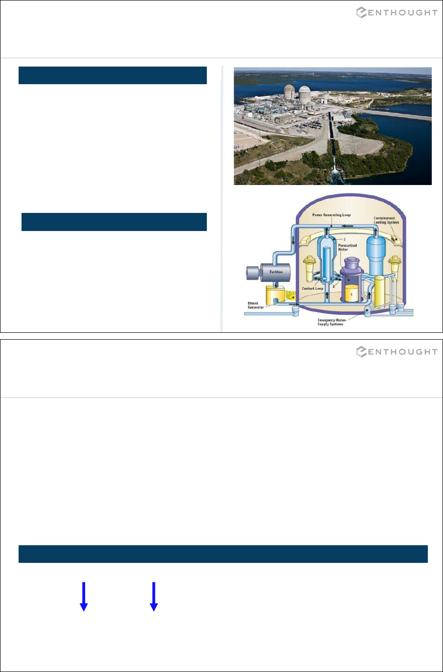
Modeling a Power Plant
# Data that describes the
# modeled "object"
name: Comanche Peak
maximum_output: 2.3 Gigawatts
current_output: ? Gigawatts
status: normal
night_watchman: Homer Simpson (!)
...
ATTRIBUTES
BEHAVIORS (METHODS)
# tasks or operations that the
# model does.
start_up()
shut_down()
emergency_shutdown()
...
95
Creating Objects
Object oriented programming unifies (encapsulates)
attributes and behavior within a single
definition, called a Class.
Instances, or Objects, of a class are specific
manifestations of that class.
>>> plant_1 = PowerPlant(name='Comanche Peak')
# Create a 2nd instance from the same class
>>> plant_2 = PowerPlant(name='Susquehanna')
INSTANTIATING CLASS INSTANCES (OBJECTS)
Class Instance

96
Working with Objects
# Our befuddled friend.
>>> homer = Person(first='Homer', last='Simpson')
# Create the power plant he is in charge of...
>>> plant = PowerPlant(name='Comanche Peak', maximum_output=2.3,
night_watchman=homer)
# Start the plant using the 'start_up' method.
>>> plant.start_up()
# Homer does his thing.
>>> homer.eat('donut')
>>> homer.take_nap()
# Check the status (an attribute) of
# the plant. No Bueno.
>>> if plant.status != 'normal':
... print 'status:', plant.status
... homer.speak('Doh!')
... plant.emergency_shutdown()
status: meltdown
Homer says 'Doh!'
97
Class Definition
class PowerPlant(object):
# Constructor method
def __init__(self, # self is ALWAYS the first argument.
name='', maximum_output=0.0, night_watchman=None):
# assign passed-in arguments to new object
self.name = name
self.maximum_output = maximum_output
self.night_watchman = night_watchman
# Intialize other attributes.
self.current_output = 0.0
self.status = 'normal'
# class methods
def start_up(self):
self.start_reactor_cooling_pump()
self.reduce_boric_acid_concentration()
self.remove_control_rods()
def shut_down(self):
...
<other methods>

98
Object Creation Process
# What does Python do when it sees this line of code?
>>> plant = PowerPlant(name='Comanche Peak', maximum_output=2.3,
night_watchman=homer)
CREATING A CLASS OBJECT
# The first step is to call the PowerPlant class' "magic"
# __new__ method to create the object. (This is a secret…)
new_object = PowerPlant.__new__(PowerPlant,
name='Comanche Peak',
maximum_output=2.3,
night_watchman=homer)
# The second step is to call the magic "constructor" method, __init__.
# This is the method you will need to write...
PowerPlant.__init__(new_object,
name='Comanche Peak',
maximum_output=2.3,
night_watchman=homer)
# Python hands this newly created object back to you.
plant = new_object
UNDER THE COVERS…
99
Particle Class Example
>>> class Particle(object):
... # Initializer method
... def __init__(self, m, v):
... self.mass = m # Assign attribute values of new object
... self.velocity = v
... # Method for calculating object momentum
... def momentum(self):
... return self.mass * self.velocity
... # A "magic" method defines object's string representation.
... # Evaluating the repr recovers the Particle object.
... def __repr__(self):
... return "Particle({0}, {1})".format(
... repr(self.mass), repr(self.velocity))
SIMPLE PARTICLE CLASS
EXAMPLE
>>> a = Particle(3.2, 4.1)
>>> print a.momentum()
13.12
>>> a
Particle(3.2, 4.1)
100
Overloading Addition
... def __add__(self, other)
... if not isinstance(other, Particle):
... return NotImplemented
... mnew = self.mass + other.mass
... vnew = (self.momentum() + other.momentum())/mnew
... return Particle(mnew, vnew)
SIMPLE PARTICLE CLASS
Classes can override many behaviors using special method names —
including numeric behavior.
EXAMPLE (cont.)
>>> b = Particle(8.6, 10.2)
>>> b, a
(Particle(8.6, 10.2), Particle(3.2, 4.1))
>>> c = a + b
>>> c
Particle(11.8, 8.545762711864406)
>>> print c.momentum()
100.84
101
Inheritance
PowerPlant
NuclearPowerPlant HydroPowerPlant

102
Base Class
class PowerPlant(object):
# Constructor method
def __init__(self, # "self" is ALWAYS the first argument.
name='', maximum_output=0.0, night_watchman=None):
# assign passed-in arguments to new object
self.name = name
self.maximum_output = maximum_output
self.night_watchman = night_watchman
# Initialize other attributes.
self.current_output = 0.0
self.status = 'normal'
# Default implementation for methods
def start_up(self):
self.current_output = self.maximum_output
def shut_down(self):
self.current_output = 0.0
...
103
Sub-Classing
# Derive 'specialized' classes from the PowerPlant base class.
# They will 'inherit' the methods of the base class.
class NuclearPowerPlant(PowerPlant):
# over-ride methods that need custom behavior.
def start_up(self):
self.start_reactor_cooling_pump()
self.reduce_boric_acid_concentration()
self.remove_control_rods()
def shut_down(self):
...

104
Using Super
# Use 'super' to call the "super-class" (parent class) methods.
class HydroPowerPlant(PowerPlant):
def __init__(self, name='', river_name='',
maximum_output=0.0, night_watchman=None):
# Use 'super' to call an over-ridden method from the
# base class.
super(HydroPowerPlant, self).__init__(name=name,
maximum_output=maximum_output,
night_watchman=night_watchman)
self.river_name = river_name
# over-ride methods that need custom behavior.
def start_up(self):
self.open_sluice_gate()
self.unlock_turbine_shaft()
self.remove_control_rods()
105
Interchangeable Classes
# The same code will work without modification for a
# NuclearPowerPlant or a HydroPowerPlant.
>>> homer = Person(first='Homer', last='Simpson')
# Create the power plant he is in charge of...
>>> plant = HydroPowerPlant(name='Comanche Peak', maximum_output=2.3,
night_watchman=homer)
# Start the plant using the 'start_up' method.
>>> plant.start_up()
# Homer does his thing.
>>> homer.eat('donut')
>>> homer.take_nap()
# Check the status (an attribute) of the plant. No Bueno.
>>> if plant.status != 'normal':
... print 'status:', plant.status
... homer.speak('Doh!')
... plant.emergency_shutdown()
status: Fish stuck in impeller.
Homer says 'Doh!'

106
Advanced Python Topics
107
Properties

108
Properties: an example
>>> a = MyNumberA(number=13)
>>> a.number
13
>>> a.number = 200
>>> a.number
200
>>> a.set_number('0xFF')
>>> a.number
255
>>> a.number = '0xFFFF' # !!!
>>> a.number
‘0xFFFF’
The set_number method allows
the value to be an integer or a
hex or binary string (e.g. ‘0xFF’
or ‘0b1101’).
# my_number.py
class MyNumberA(object):
def __init__(self, number):
self.number = number
def set_number(self, value):
if isinstance(value, basestring):
self.number = eval(value)
else:
self.number = value
109
Properties: definition
Wouldn’t this be nice?
>>> a.number = '0xFFFF'
>>> a.number
65535
>>> a.number = '0b1101'
>>> a.number
13
The number magically converts a hex string or a binary string to the integer value.
We can do this, by creating a property. A property allows us to implement something
that acts like an attribute, but attempting to get or set a value of the attribute actually results
in a function call. property() is a built-in function in Python.
property(fget=None, fset=None, fdel=None, doc=None)

110
Properties: application 1
>>> b = MyNumberB(number=100)
>>> b.number
100
>>> b.number = '0xFF'
>>> b.number
255
>>> b.number = '0b1101'
>>> b.number
13
# my_numberB.py
class MyNumberB(object):
def __init__(self, number):
self._number = number
def _get_number(self):
return self._number
def _set_number(self, value):
if isinstance(value, basestring):
number = eval(value)
else:
number = value
self._number = number
number = property(_get_number, _set_number)
111
Properties: application 2
For example, the energy and momentum methods of the Particle class can be
implemented as read-only properties:
# My_particle_class.py
class Particle(object):
…
def _get_momentum(self):
return self.mass * self.velocity
def _get_energy(self):
return 0.5 * self.mass * self.velocity**2
def _not_allowed(self, value):
raise RuntimeError("Can not set energy or momentum
directly.")
energy = property(_get_energy, _not_allowed)
momentum = property(_get_momentum, _not_allowed)

112
Properties
Then, for example:
>>> p = Particle(mass=3.0, velocity=4.0)
>>> p.momentum
12.0
>>> p.energy = 100
Traceback (most recent call last):
File "<stdin>", line 1, in <module>
File "particle_with_properties.py", line 23, in _not_allowed
raise RuntimeError("can not set energy or momentum directly.")
RuntimeError: can not set energy or momentum directly.
113
General Scoping Rules
•Local Function Scope
•Enclosing Function Scope
•Global Scope
•Builtin Scope
Variables are looked up from
namespaces in the following order:

114
Scoping Rules
# If a requested variable is not
# found in the local scope, the
# "global" or module level scope
# is searched.
# global module level variable
c = 1
def foo(a,b):
d = a + b + c
LOCAL SCOPE
GLOBAL SCOPE
MODIFYING GLOBALS
# a, b, c and d are all local
# variables in the function.
def foo(a,b):
c = 1
d = a + b + c
# Modifying globals from within
# a local scope requires the
# global keyword.
c = 1
def foo():
global c
c = 2
>>> foo()
>>> print c
2
115
Scoping Rules
BUILTIN SCOPE
# If not found in the local or
# global scope, the "builtin"
# scope is searched. 'len' is
# a builtin function.
def list_length(a):
return len(a)
>>> a = [1,2,3]
>>> print list_length(a)
3
# The "builtin" functions are
# found in the special
# __builtin__ module
>>> import __builtin__
>>> __builtin__.len
<built-in function len>

117
Class Scoping Rules
# global variable
var = 0
class MyClass(object):
# class variable
var = 1
def access_class_c(self):
print 'class var:', self.var
def access_global_c(self):
print 'global var:', var
def write_class_c(self):
# Modify the class variable.
MyClass.var = 2
print 'class var:', self.var
def write_instance_c(self):
# Create an instance variable.
self.var = 3
print 'instance var:', self.var
See
demo/variable_scoping/class_
scoping.py.
>>> obj = MyClass()
>>> obj.access_class_c()
class var: 1
>>> obj.access_global_c()
global var: 0
>>> obj.write_class_c()
class var: 2
>>> obj.write_instance_c()
instance var: 3
CLASS SCOPING EXAMPLES
118
Lexical Scoping Rules
NESTED SCOPE FUNCTION CLOSURE
# Nested functions have access
# to the enclosing function’s
# variables.
def outer():
a = 1
def inner():
print "a =", a
inner()
>>> outer()
a = 1
# The inner() function has access
# to the outer variables that it
# uses for its entire lifetime.
def outer():
a = 1
def inner():
return a
return inner #Note: returns
#function object!
>>> func = outer()
>>> print 'a (1):', func()
a (1): 1
See
demo/variable_scoping/lexical
_scoping.py.

119
Partial Function Application (or Curries)
PARTIAL
# functools.partial "freezes"
# one or more arguments of a
# function to create a simplified
# signature and/or modify default
# arguments.
# By default, int uses base 10
# conversion from string to int.
>>> int('10010')
10010
# Create function to convert
# base 2 strings to ints.
>>> from functools import partial
>>> basetwo = partial(int, base=2)
>>> basetwo('10010')
18
120
Decorators

121
Func as objects and arguments
Passing Functions Function Objects
>>> def foo(x):
... print x
# foo is of type ‘function’.
>>> type(foo)
<type 'function'>
# Functions have a set of
# attributes, like other objects.
>>> dir(foo)
['__call__', ..., 'func_closure’,
'func_code', 'func_defaults’,
'func_dict', 'func_doc',
'func_globals’, 'func_name']
# __call__ is the most important
>>> foo(42)
42
In Python, functions are first-class objects.
# Since functions are objects,
# like everything else in Python,
# they can be passed as arguments
# to other functions!
>>> def foo(x):
... print x
...
>>> def bar(f, x):
... x += 1
... f(x)
...
>>> bar(foo, 42)
43
Note: Python has a ‘lambda’
keyword for defining anonymous
functions inline.
122
Decorators
# A basic decorator
>>> def dec(f):
... print "I am decorating function ", id(f)
... return f
>>> declen = dec(len)
I am decorating function 2338768
>>> declen([10, 20, 30])
3
Decorators are functions which take a function as an argument and
(usually) return another function.
Example

123
Decorators
# Makes a new function that will loudly call the original.
# Note the definition of new_func inside the definition of
# loud.
>>> def loud(f):
... def new_func(*args, **kw):
... print "Calling with", args, kw
... rtn = f(*args, **kw)
... print "Return value is", rtn
... return rtn
... return new_func
>>> loudlen = loud(len) # Create a modified len().
>>> n = loudlen([10, 20, 30]) # Call it.
Calling with ([10, 20, 30],) {}
Return value is 3
>>> n
3
Example
124
Decorators
# Given a decorator dec’, the phrasing...
def foo(x):
print x
foo = dec(foo)
# can be replaced by...
@dec
def foo(x):
print x
# If the decorator returns a function,
# decorations may be chained.
@dec1
@dec2
def foo(x):
print x
Python uses the ‘@’ symbol to replace a function with its decorated version.
@ Notation

125
Decorator Examples
# A decorator that adds 1
def plus_one(f):
def new_func(x):
return f(x) + 1
return new_func
# A decorator that multiplies by 2
def times_two(f):
def new_func(x):
return f(x) * 2
return new_func
# A decorated function
@plus_one
@times_two
def foo(x):
return int(x)
>>> foo(13)
27
126
Decorator Factories
# A basic decorator generator
def super_dec(x, y, z):
# The decorator we are creating
def dec(f):
# The function to return
def new_func(*args, **kw):
print x + y + z
return f(*args, **kw)
return new_func
return dec
If you want to change the behavior of the decorator when you decorate, you
do this by writing a decorator factory. A factory is a function that returns a
decorator.

127
Decorator Factory Example
# Appends a string to the function output
def append_string(s):
def dec(f):
def new_func(*args, **kw):
new_s = f(*args, **kw) + s
return new_s
return new_func
return dec
@append_string(", World")
def hello():
return "Hello"
>>> hello()
Hello, World
@append_string(", Moon")
def goodnight():
return "Goodnight"
>>> goodnight()
Goodnight, Moon
128
Iterators, generators and
coroutines

129
Iterators
class FootballRushIterator(object):
def __init__(self, count=5):
self.count = count
def __iter__(self):
# Prepare an iterable object.
self._counter = 1
return self
def next(self):
cnt = self._counter
if cnt <= self.count:
# Return the next element
res = str(cnt) + " mississippi"
self._counter += 1
return res
else:
# Or signal the end of iteration.
raise StopIteration
(WITH GENERATOR)
CLASS DEFINTION
>>> rusher = FootballRushIterator()
>>> for count in rusher:
... print count
1 mississippi
2 mississippi
3 mississippi
4 mississippi
5 mississippi
Iterators are anything that can be looped over. They shield users from
implementation details of looping over an object. Classes that have __iter__ and
next methods can be used as iterators.
def get_rusher(count=5):
for i in range(count):
yield "%d mississippi" % (i+1,)
>>> for count in get_rusher():
... print count
USING ITERATORS
130
Generators
def simple_generator():
print 'first'
yield 1
print 'second'
yield 2
>>> sequence = simple_generator()
>>> sequence.next()
first
1
>>> sequence.next()
second
2
>>> sequence.next()
Traceback (most recent call last):
File "<stdin>" line 1, in ?
StopIteration
USING GENERATORS GENERATOR BASICS
# Create a generator that returns the
# first N elements of the Fibonacci
# sequence.
def fib(N=10):
a, b = 0, 1
for count in range(N):
yield b
a, b = b, a+b
>>> fib_gen = fib(6)
>>> for value in fib_gen:
print value
1
1
2
3
5
8
Generators are a special kind of function that contain a yield statement. These
functions are really iterator factories. The returned iterator can be looped over or
its next() method can be called directly to return elements from the sequence.

131
Generators --> CoRoutines
def receiving_generator():
while True:
val = (yield)
print "Received", val
>>> sequence = receiving_generator()
# First next() call take to the first
# yield
>>> sequence.next()
>>> sequence.next()
Received None
>>> sequence.send(1)
Received 1
>>> sequence.send("hello")
Received hello
>>> sequence.close()
EMITTING AND RECEIVING COROUTINES BASICS
Generators can receive values as well using the return value of a yield
expression: they are called coroutines.
def emiting_receiving_generator():
i = -1
while True:
i += 1
val = (yield i)
print "Received", val
>>> sequence = receiving_generator()
>>> sequence.next()
0
>>> sequence.next()
Received None
1
>>> sequence.send("hello")
Received hello
2
>>> sequence.close()
132
Context managers and the with
statement

Introduction
• New in python 2.5, though it’s then required to import it:
from __future__ import with_statement
•Context managers are objects that possess the
__enter__ and __exit__ methods. They are used to
define a sequence of setup and tear-down operations
that the with statement will call automatically even if
exceptions are raised, similar to a try/finally block.
•An example of a context manager is the file pointer
which includes f.close() in its __exit__ method.
133
Example
134
class MyContext(object):
def __enter__(self):
print "I entered"
return self
def __exit__(self, type, value, tb):
print("Exception info: %s, %s, %s" % (type, value, tb)
print "Before exiting important things to do... ”
CONTEXT CREATION
>>> with MyContext() as c:
... print "I am doing things..."
... raise RuntimeError("Crash!")
I entered
I am doing things...
Exception info: ’RuntimeError’,
Crash!, <traceback object at 0x824>
Before exiting important things
to do...
RuntimeError: Crash!
>>> c
<__main__.MyContext at
0xa3c09b0>
USING THE CONTEXT

135
Dynamic Code Execution
EVAL EXEC
# The "eval" function will
# evaluate a Python expression
# within a given global and local
# namespace (dictionary).
# Both the global and local
# dictionary are optional.
# eval(expr, globals, locals)
>>> a = 1
>>> eval("a+1")
2
# Specify a local dictionary.
>>> local = dict(a=2)
>>> glob = {}
>>> eval("a+1", glob, local)
3
# The "exec" statement will
# execute a Python statement
# within a given global and
# local namespace (dictionary).
# Both the global and local
# dictionary are optional.
# exec(stmt, globals, locals)
>>> a = 1
>>> exec("b = a+1")
>>> print b
2
# Specify a local dictionary.
>>> local = dict(a=2)
>>> glob = {}
>>> exec("b=a+1", glob, local)
>>> print local
{'a': 2, 'b': 3}
Careful about eval’ing/exec’ing an untrusted user’s input: they have full
access to python.
136
exec with a dictionary-like namespace
EXEC
class LoudDict(dict):
""" This dictionary announces whenever one of its values
is get or set.
"""
def __getitem__(self, key):
value = super(LoudDict, self).__getitem__(key)
print "retrieving %s which is %s" % (key, value)
return value
def __setitem__(self, key, value):
print "setting %s = %s" % (key, value)
super(LoudDict, self).__setitem__(key, value)
# Execute a statement in our "LoudDict" and watch it announce
# variable get/set during the execution.
>>> local = LoudDict(a=1)
>>> exec "b=a+1" in {}, local
retrieving a which is 1
setting b = 2
See demo/dictionary_like_exec.py

137
Dynamic ByteCode Generation
COMPILE
# The ”compile" function will generate bytecode from a Python
# expression or statement. It can then be evaluated multiple
# times without regenerating the bytecode each time.
# Syntax: compile(str, filename, mode)
>>> a = 1
>>> c=compile("a+2", "", "eval")
>>> eval(c)
3
>>> c=compile("b=a+2", "", "exec")
>>> exec(c)
>>> b
3
>>> a = 3
>>> exec(c)
>>> b
5
Careful about eval’ing/exec’ing an untrusted user’s input: they have full
access to python.
138
csv – read and write CSV files
The csv modules provides classes for reading and writing Comma Separated
Value (CSV) files.
csv.reader - Read a list of comma-separated values from a file.
csv.writer - Output a list (or other iterable) to a file.
The format is configurable; in particular, the data delimiter does not have to be
a comma.
Default “dialect” is compatible with Excel.

139
csv examples
Sample data file “data.csv”:
"alpha 1", 100, -1.443
"beta 3", 12, -0.0934
"gamma 3a", 192, -0.6621
"delta 2a", 15, -4.515
>>> import csv
>>> rdr = csv.reader(
open("data.csv"))
>>> for row in rdr:
... print row
['alpha 1', ' 100', ' -1.443']
['beta 3', ' 12', ' -0.0934']
['gamma 3a', ' 192', ' -0.6621']
['delta 2a', ' 15', ' -4.515']
>>> import csv
>>> data = [("One", 1, 1.5),
("Two", 2, 8.0)]
>>> f = open("out.csv", "w")
>>> wrtr = csv.writer(f)
>>> wrtr.writerows(data)
>>> f.close()
One,1,1.5
Two,2,8.0
Output file “out.csv”:
READER WRITER
140
csv options
delimiter: str (a single character)
The field separator character
doublequote: bool
If True, a quote inside a string is doubled.
If False, prefix the quote with escapechar.
escapechar: str (a single character)
The character that indicates the following
character has no special meaning.
quotechar: str (a single character)
Character used to quote strings containing
delimiters or other special characters.
quoting: one of csv.QUOTE_* constants
Controls when quotes should be generated
by the writer and recognized by the reader.
>>> data
[('One', 1, 1.5), ('Two', 2, 8.0)]
>>> f = open("out.txt", "w")
>>> wrtr = csv.writer(f,
delimiter='|',
quoting=csv.QUOTE_ALL)
>>> wrtr.writerows(data)
>>> f.close()
"One"|"1"|"1.5"
"Two"|"2"|"8.0"
OPTIONS (not a complete list) EXAMPLE
Output file “out.csv”:

141
Connecting to Databases
142
DB-API 2.0
PEP (Python Enhancement Proposal) 249 detailed version
2.0 of the DB-API to promote consistency between
Python front-ends to data-bases.
Database
Module
or Modules for Python 2.X
Oracle cx_Oracle, DCOracle2, mxODBC, pyodbc
PostgreSQL psycopg2, PyGreSQL, pyPgSQL, mxODBC, pyodbc, pg8000
MySQL MySQLdb, mxODBC, pyodbc, myconnpy
Sqlite sqlite3 (included in standard library)
Microsoft SQL Server adodbapi, pymssql, mssql, mxODBC, pyodbc
Ingres ingresdbi
IBM DB2 Ibm_db, PyDB2, ceODBC, mxODBC, pyodbc
Sybase ASE Sybase, mxODBC
Sybase SQL Anywhere mxODBC, sqlanydb
SAP DB sdb.dbapi, sapdbapi, mxODBC, sdb.sql, sapdb
Informix InformixDB, mxODBC,
Firebird KInterbasdb
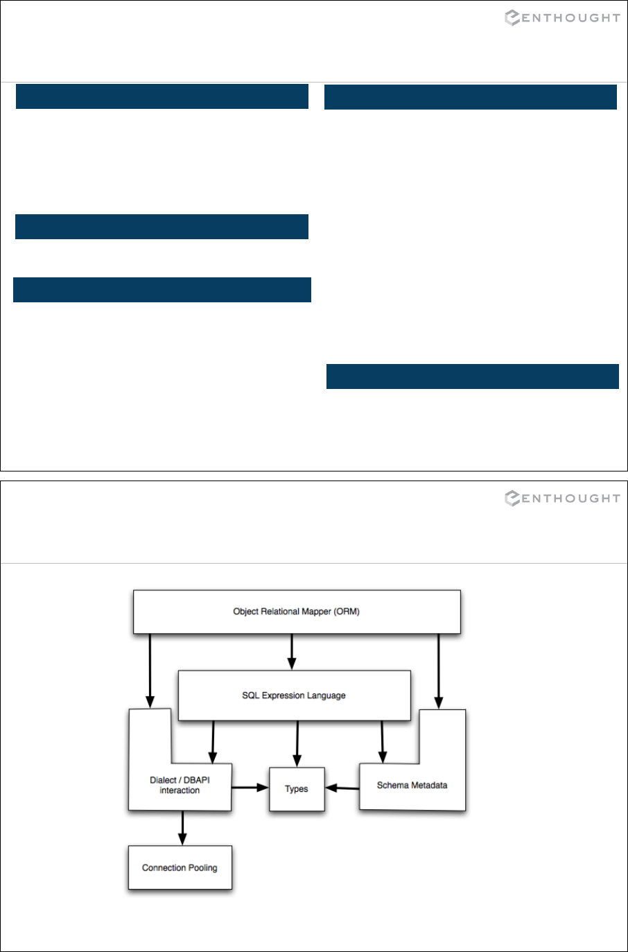
143
DB-API 2.0
Connect to the database
Get a cursor object
Execute SQL statements
Execute SQL Statements (cont.)
Close cursor and connection
import <somedbmodule> as db
# Connect to the data-source
# Extra arguments typically
# include user and password
conn = db.connect(<dsn>,…)
c = conn.cursor()
c.execute(“create table stocks(date
text, trans text, symbol text, qty real,
price real)”)
c.execute(“insert into stocks values
('2006-01-05','BUY','RHAT',100,35.14)”)
conn.commit() c.close()
conn.close()
t = ('2006-04-06', 'SELL',
'IBM', 500, 53.00)
c.execute(“insert into stocks values
(?,?,?,?,?)”, t)
# some modules use a different
# place-holder instead of ?
# see db.paramstyle
t = (‘IBM’,)
c.execute(“select * from stocks where
symbol=? order by price”, t)
for row in c:
print row
single = c.fetchone()
list_of_lists = c.fetchall()
144
An ORM: SQLAlchemy

146
Regular Expressions
in Python
147
What is a regular expression?
A regular expression is a pattern designed to match
specific strings or sub-strings.
A regular expression can match very specific strings, as
well as very general strings.
Once matched, specific fields in the string can be extracted
or substituted. Information about the location, and type
of match is stored in a match object.

148
>>> import re
Some of the more common uses of the re API
>>> re.match(pattern, string[, flags])
>>> re.search(pattern, string[, flags])
Matches (or search) the pattern against the string, returning a match object on
success and None on failure (flags described later). re.match only searches for a
match at the beginning of the string. re.search will search through the entire string.
>>> re.findall(pattern, string)
Returns a list of matches of pattern in string. re.finditer returns an iterator.
>>> re.split(pattern, string[, maxsplit])
Returns a list of sub-strings, delimited by the regular expression pattern. If maxsplit
is specified only maxsplit splits will occur.
>>> re.sub(pattern, repl, string[, count])
Returns a string where every occurrence matching the regular expression pattern in
string is replaced by repl, unless count is reached (specifies how many
substitutions to make).
>>> re.compile(pattern)
Compiles the regex and returns a pattern object which can be used for searching,
matching, substituting, …. match, search, findall … are then methods of the object.
149
Regular expression syntax
. Matches any character except newline
\w Matches any alphanumeric character
\d Matches any decimal digit, equal to [0-9]
\s Matches whitespace, equal to [ \t\n\r\f\v]
[…] Indicates a set of characters which can
be matched. Ranges can be specified
using - (e.g. a-z, 0-9).
(...) Groups characters/symbols into 1 block
| Stands for logical OR
^ Takes the complement of the following set
* Causes the previous RE to match zero
or more repetitions
+ Matches 1 or more repetitions of the
previous RE
? Matches zero or 1 occurrences of the
previous RE
{
m
} Matches
m
occurrences of the previous
RE
A regex pattern is composed of regular characters as well as various symbols for
matching patterns in strings...below are some of the common symbols.
\D \S and \W denote the
complement of the same sets
For e.g., ca*t matches ‘ct’, ‘cat’, ‘caaaat’, …
(ab\d)|(ac\d) matches ‘ab1’, ‘ac9’, …
([^a-q]bd) matches ‘rbd’, ‘5bd’, …
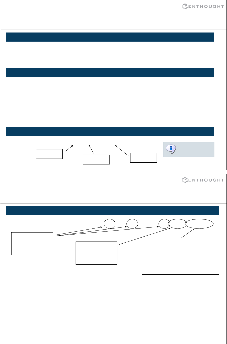
150
Match objects & groups
When a regular expression matches, a match object is returned.
>>> myString = "hello world"
>>> print re.match("hello (\w+)", myString)
<_sre.SRE_Match object at 0x009E45E0>
Check if a match was successful, extract matched groups, location, …
>>> myString = "hello there"
>>> match = re.match("hello (\w+)", myString)
>>> if match != None:
... print match.group(1)
'there'
>>> print match.start, match.end
6 11
Groups are numbered left to right, based on open parenthesis...
>>> re.match("hello (\w+(\d+)*) (\w+)", myString)
Group 1 Group 2 Group 3
Nested groups
count too!
151
Regular expression example
compile() return a re pattern object
>>> patt1 = re.compile("hello\s+user\s+number\s+(\d+)(\.\d+)*")
Match one or
more space
characters First group will
match 1 or
more digits
2nd group will match an
optional dot then 1 or more
digits. Optional because of *,
dot is escaped with \ since it
is a special symbol
>>> patt1 = re.compile("hello\s+user\s+number\s+(\d+)(\.\d+)*")
>>> s1 = "hello user number 87"
>>> s2 = "hello user number 87.34“
>>> m = patt1.match(s1)
>>> print m.group(1)
'87'
>>> m = patt1.match(s2)
>>> print m.groups()
('87', '.34')
152
Parse the following text to extract the
number and the type of all travellers:
"5 men, 7 dogs and 12 goats are
travelling together."
Exercise
153
A note about parsing XHTML
Source: http://stackoverflow.com/questions/1732348/regex-match-open-tags-except-xhtml-self-contained-tags

154
NumPy’s fromregex
NumPy contains a function fromregex that can be used to convert arbitrary
text files to (structured) arrays.
data = fromregex(file, pattern, dtype)
file: file-like object or filename string.
pattern: Regular expression to parse file with.
Groups must correspond to fields in the
dtype.
dtype: data-type for the structured array with
field for each group in the regular
expression.
Output is a structured array where each element is a
match to the regular expression in the file.
155
fromregex example
# Create the file
>>> f = open('test.dat', 'w')
>>> f.write("1312 foo\n1534 bar\n444 qux")
>>> f.close()
# match [digits, whitespaces, anything]
>>> regexp = "(\d+)\s+(...)"
>>> output = fromregex('test.dat', regexp,
... [('num’,np.int64),('key','S3')])
>>> output
array([(1312L, 'foo'), (1534L, 'bar'), (444L, 'qux')],
dtype=[('num', '<i8'), ('key', '|S3')])
>>> output['num']
array([1312, 1534, 444], dtype=int64)

156
datetime – Dates and Times
TIME OBJECT DATE OBJECT
# date(year, month, day)
# date in Gregorian calendar,
# assuming its permanence
>>> d1 = date(2007, 9, 25)
>>> d2 = date(2008, 9, 25)
>>> d1.strftime('%A %m/%d/%y')
'Tuesday 09/25/07'
# difference is timedelta
>>> print d2 – d1
366 days, 0:00:00
>>> (d2-d1).days
366
>>> print date.today()
2008-09-24
>>> from datetime import date, time
# time(hour, min, sec, us)
# local time of day
# always 24 hrs per day
>>> t1 = time(15, 38)
>>> t2 = time(18)
>>> t1.strftime('%I:%M %p')
'03:38 PM'
# difference is not supported
>>> print t2 – t1
Traceback ...
TypeError: unsupported operand ...
# use datetime objects for
# difference operation.
157
datetime – Dates and Times
DATETIME OBJECT
# datetime(year, month, day,
hr, min, sec, us)
# combination of date and time
>>> d1 = datetime.now()
>>> print d1
2008-09-24 14:20:30.978207
>>> d2 = d1 + timedelta(30)
>>> d2.strftime('%A %m/%d/%y')
'Friday 10/24/08'
# creating datetime from
# a format string
>>> datetime.strptime('2/10/01',
'%m/%d/%y')
datetime.datetime(2001, 2, 10, 0, 0)
>>> from datetime import datetime, timedelta
Directive Meaning
%a (%A) Abbrev. (full) weekday
name.
%w Weekday number [0(Sun),6]
%b (%B) Abbrev. (full) month name
%d Day of month [01,31]
%H (%I) Hour [00,23] ([01,12])
%j Day of the year [001,366]
%m Month [01,12]
%M Minute [0,59]
%p AM or PM
%S Second [00,61]
%U (%W) Week number of the year
[00,53] Sunday (Monday) as
first day of week.
%y (%Y) Year without (with)
century [00,99]
DATETIME FORMAT STRING

158
Context managers and the with
statement
Introduction
• New in python 2.5, though it’s then required to import it:
from __future__ import with_statement
•Context managers are objects that possess the
__enter__ and __exit__ methods. They are used to
define a sequence of setup and tear-down operations
that the with statement will call automatically even if
exceptions are raised, similar to a try/finally block.
•An example of a context manager is the file pointer
which includes f.close() in its __exit__ method.
159

Example
160
class MyContext(object):
def __enter__(self):
print "I entered"
return self
def __exit__(self, type, value, tb):
print("Exception info: %s, %s, %s" % (type, value, tb)
print "Before exiting important things to do... ”
CONTEXT CREATION
>>> with MyContext() as c:
... print "I am doing things..."
... raise RuntimeError("Crash!")
I entered
I am doing things...
Exception info: ’RuntimeError’,
Crash!, <traceback object at 0x824>
Before exiting important things
to do...
RuntimeError: Crash!
>>> c
<__main__.MyContext at
0xa3c09b0>
USING THE CONTEXT
161
sys module
>>> import sys
Some frequently used attributes and functions—see the
reference manual for complete details.
sys.argv
List of command line arguments.
sys.argv[0] is the name of the python script.
Example:
sys.exc_info()
Returns a tuple (type, value, traceback)
sys.exc_clear()
Clear all exception information.
Command Line Arguments Exception Information
# File: print_args.py
import sys
print sys.argv
$ python print_args.py 1 foo
['print_args.py', '1', 'foo']
>>> try:
... x = 1/0
... except Exception:
... print sys.exc_info()
...
(<type 'exceptions.ZeroDivisionError'>,
ZeroDivisionError('integer division or
modulo by zero',), <traceback object at
0x9a8c8>)
>>>

162
sys module
sys.exit(arg)
Exit from Python. arg is optional. It can be an
integer giving the exit status (defaults to zero).
If not an integer, None is equivalent to passing
0, and any other argument is printed to
sys.stderr and the exit status is 1.
sys.stdin
sys.stdout
sys.stderr
The interpreter’s standard input, output and
error streams.
sys.__stdin__
sys.__stdout__
sys.__stderr__
The original values of sys.stdin, sys.stdout
and sys.stderr at the start of the program.
Exit Standard File Objects
Python’s module search path
sys.path
A list of strings that specifies the interpreter’s
search path for modules.
A program is free to modify this list
dynamically.
163
sys module
sys.version
A string containing information
about the Python version.
sys.version_info
A tuple containing information about
the Python version: major, minor,
micro, releaselevel and serial.
>>> sys.version
'2.6.5 |EPD 6.2-2 (32-bit)|
(r265:79063, May 7 2010, 13:28:19)
[MSC v.1500 32 bit (Intel)]'
>>> sys.version_info
(2, 6, 5, 'final', 0)
sys.platform
A string containing the platform identifier.
Windows: ‘win32’
Mac OSX: ‘darwin’
Linux: ‘linux2’
sys.getwindowsversion()
Return a tuple that describes the version of
Windows currently running: major, minor,
build, platform, and service_pack. (More is
included in Python 2.7.)
>>> sys.platform
‘win32’
>>> sys.getwindowsversion()
(5, 1, 2600, 2, ‘Service Pack 3’)
Python Version Platform Information
See also the platform module in the
standard library.

164
os module
>>> import os
os.remove(path) os.unlink(path)
Remove a file from disk (file can be
either the full path or a file from the
current working directory will be
removed.
os.chdir(path)
Change the current working directory to
the provided path.
os.getcwd()
Return the current working directory.
os.listdir(path)
Return a list of strings containing all the
files in the given path (does not include '.‘
or '..' in the listing).
os.linesep (e.g. '\n' or '\r\n')
Line separator in text mode.
os.sep (e.g. '/' or '\')
Path separator on file system.
os.pathsep (e.g. ':' or ';')
Search path separator (i.e. in
environment variables).
Path Operations Separation Constants
os.environ
Dictionary of all environment variables
os.urandom(len)
String of random bytes
os.error
Error object
Others
165
os.path
os.path.isfile(path)
Test whether a path is a regular file.
os.path.isdir(path)
Test whether a path refers to an existing
directory.
os.path.exists(path)
Test whether a path exists.
os.path.isabs(path)
Test whether a path is absolute.
os.path.abspath(path)
Return an absolute path.
os.path.dirname(path)
Return the directory component of a
pathname.
os.path.basename(path)
Return the final component of a
pathname.
os.path.splitext(path)
Split the extension from a pathname.
Returns (root, ext).
os.path.expanduser(path)
Expand ~ and ~user. If user or $HOME is
unknown, do nothing.
os.path – tests Others
os.path – split and join
os.path.split(path)
Split a pathname. Returns the tuple
(head, tail).
os.path.join(a, *p)
Join two or more path components.

166
Remote Call example — xmlrpc
from SimpleXMLRPCServer import SimpleXMLRPCServer
def fact(n):
if n <= 1:
return 1
else:
return n * fact(n-1)
# Start a server listening for requests on port 8001.
if __name__ == '__main__':
server = SimpleXMLRPCServer((‘localhost', 8001))
# Register fact as a function provided by the server.
server.register_function(fact)
server.serve_forever()
>>> import xmlrpclib
>>> svr = xmlrpclib.Server("http://localhost:8001")
>>> svr.fact(10)
3628800
CLIENT CODE — CALLS REMOTE FACTORIAL FUNCTION
XMLRPC FACTORIAL SERVER – VERSION 1
167
Remote Call example — xmlrpc
from SimpleXMLRPCServer import SimpleXMLRPCRequestHandler, \
SimpleXMLRPCServer
def fact(n):
if n <= 1: return 1
else: return n * fact(n-1)
# Override the _dispatch() handler to call the requested function.
class my_handler(SimpleXMLRPCRequestHandler):
def _dispatch(self, method, params):
print "CALL", method, params
return apply(eval(method), params)
# Start a server listening for requests on port 8001.
if __name__ == '__main__':
server = SimpleXMLRPCServer((‘localhost', 8001), my_handler)
server.serve_forever()
>>> import xmlrpclib
>>> svr = xmlrpclib.Server("http://localhost:8001")
>>> svr.fact(10)
3628800
CLIENT CODE — CALLS REMOTE FACTORIAL FUNCTION
XMLRPC FACTORIAL SERVER – VERSION 2

168
Calling Subprocesses
169
Executing other programs
>>> from subprocess import Popen, PIPE, STDOUT
p = Popen([cmd,arg1,…,argn], env=None, cwd=None, shell=False,
stdin=None, stdout=None, stderr=None)
cmd,arg1,…,argn Command to run plus any arguments
stdin, stderr, stdout
Standard file handles: can be None (use
handles of the current process), any open file
descriptor, any open file object, or PIPE.
(stderr can also be STDOUT for a redirect).
env Dictionary of environment variables. If None,
then the current process environment is used.
shell Run the cmd in the shell if True
cwd Directory to change to before executing the
command.
Command begins to execute immediately!

170
Executing other programs
# On Windows
>>> Popen('dir', shell=True, cwd="c:\\")
Volume in drive C has no label.
Volume Serial Number is A080-3756
Directory of c:\
08/30/2007 … AUTOEXEC.BAT
08/30/2007 … CONFIG.SYS
…
01/24/2009 … Python25
01/24/2009 … WINDOWS
2 File(s) 0 bytes
7 Dir(s) 1,401,319,424 bytes free
# On Unix (no shell needed)
>>> fid = open('simple.txt','w')
>>> Popen('ls', cwd='/usr', stdout=fid)
>>> fid.close()
bin
games
include
lib
lib32
lib64
local
sbin
share
src
X11R6
SIMPLE COMMAND EXECUTION
simple.txt
171
Executing other programs
WAIT FOR TERMINATION POLL PERIODICALLY
from subprocess import Popen
print "Starting..."
# sleep for 10 seconds
p = Popen(['sleep','10'])
# wait to finish
# and get return code
ret = p.wait()
# return code also stored
# in subprocess object
# after completion
print "Done", p.returncode
Starting
<10 seconds later>
Done 0
from subprocess import Popen
import sys
print "Starting..."
# sleep for 10 seconds
p = Popen(['sleep','10'])
# continue on with processing
print "Continuing",
k=0
while p.poll() is None:
k += 1
if (k % 100000) == 0:
print k//100000,
sys.stdout.flush()
print
print "Done", p.returncode
Starting
Continuing 1 2 3 … 45
Done 0

172
Executing other programs
# Setup process which will receive
# stdin through a PIPE and send
# stdout to a PIPE
>>> p = Popen(['python', 'count.py',
'c'], stdin=PIPE, stdout=PIPE,
stderr=PIPE)
>>> instr = "gatccatgca"
>>> out, err = p.communicate(instr)
>>> print out
3
>>> shlex.split('python count.py c’)
['python', 'count.py', 'c']
import sys
letter = sys.argv[1]
data = sys.stdin.read()
print data.count(letter)
count.py
PIPES
"Pipes" are used to send and/or receive data from another process on the same
machine.
SHLEX TO CREATE COMPLEX COMMAND
173
Multiprocessing

174
What is Multiprocessing?
The multiprocessing module provides access to task-based parallel
computing using separate Python processes.
Multiprocessing has several features:
•part of Python’s standard library,
•cross-platform,
•low-level parallel constructs: locks, queues, pipes, semaphores, shared memory
access
•higher-level constructs: task pools with automatic scheduling, shared memory
object wrappers, functional and iterator-like design support, etc.
The multiprocessing module is useful for:
•batch computing, embarrassingly parallel computations
•parallel computing with minimal shared state
•GUI programming: do calculations in a background process
•many, many others.
http://docs.python.org/library/multiprocessing.html
175
Multiprocessing vs. Threading
The threading module provides thread-based parallelism to Python; in CPython,
threads are limited by the Global Interpreter Lock.
Only one thread may hold the lock at any point in time, holding the lock allows
that thread to execute Python instructions.
Multiprocessing provides a way around this performance limitation.
The multiprocessing module has a nearly identical API to the threading module;
this is intentional.
Learn multiprocessing, you will learn majority of threading.
Primary differences:
•Threads share the same address space as the spawning thread, whereas
processes have separate address spaces.
•often more communication is required with processes; shared memory
can mitigate.
•Spawning new processes is generally more expensive (memory, time) than
spawning new threads.
•Trivial API differences.

176
The Process Class
Process(target, name=None, args=(), kwargs={})
target: a callable object, called when the start() method is called
name: string, name to give to the process; default given if None
args: tuple, arguments to pass to the target when called
kwargs: dict, keyword args to pass to the target
The basic methods for Process objects are:
start(): start the process’ activity
join([timeout]): block the calling process until the process finishes, or until
timeout
is_alive(): True if process is still running, false otherwise
terminate(): Terminate the process; may cause deadlocks, synchronization
errors, orphaned processes; use only when necessary.
The Process Class
import multiprocessing as mp
from time import sleep
from random import random
def worker(num):
sleep(2.0 * random())
name = mp.current_process().name
print "worker {},name:{}".format(num, name)
if __name__ == '__main__’:
master = mp.current_process().name
print "Master name: {}".format(master)
for i in range(2):
p = mp.Process(target=worker, args=(i,))
p.start()
# Close all child processes spawn
[p.join() for p in mp.active_children()]
CREATING A PROCESS OUTPUT
$ python basics.py
Master name: MainProcess
worker 1, name: Process-2
worker 0, name: Process-1
177

178
def worker(q):
v = q.get() # blocking!
print "got '{}' from parent".format(v)
if __name__ == '__main__':
q = mp.Queue()
p = mp.Process(target=worker, args=(q,))
p.start() # blocks at q.get()
v = 'parent'
print "putting '{}' on queue".format(v)
q.put(v)
p.join()
QUEUE BASICS
Multiprocessing provides a Queue class and a Pipe class for communicating
between processes. Queue and Pipe objects are thread and process safe.
Queue – Communicate in one direction; put() and get() methods.
Pipe – two-ended Queue, each end has a send() and recv() method.
OUTPUT
$ python queue_basic.py
putting 'parent' on queue
got 'parent' from parent
Communication Between Processes
179
Communication Between Processes
import multiprocessing as mp
def worker(p):
msg = 'whiskey tango fox trot'
print "sending {!r} to parent".format(msg)
p.send(msg)
v = p.recv()
print ”got {!r} from parent".format(v)
if __name__ == '__main__':
# The two ends of the pipe: the parent and the child connections
p_conn, c_conn = mp.Pipe()
p = mp.Process(target=worker, args=(c_conn,))
p.start()
msg = 'foobar'
print ”got {!r} from child".format(p_conn.recv())
print "sending {!r} to child".format(msg)
p_conn.send(msg)
p.join()
PIPE BASICS

Synchronization
180
import multiprocessing as mp
def print_lock(lk, i):
name = mp.current_process().name
lk.acquire()
for j in range(100):
print i, "from process", name
lk.release()
if __name__ == '__main__':
lk = mp.Lock()
ps = [mp.Process(target=print_lock,
args=(lk,i))
for i in range(100)]
[p.start() for p in ps]
[p.join() for p in ps]
Lock() objects provide a low-level way to guarantee that code is executed by only one
process at a time.
LOCK BASICS
import multiprocessing as mp
def print_lock(lk, i):
name = mp.current_process().name
with lk:
for j in range(100):
print i, "from process", name
if __name__ == '__main__':
lk = mp.Lock()
ps = [mp.Process(target=print_lock,
args=(lk,i))
for i in range(100)]
[p.start() for p in ps]
[p.join() for p in ps]
USING THE WITH STATEMENT
181
Synchronization
import multiprocessing as mp
def wait_on_event(e):
name = mp.current_process().name
e.wait()
print name, "finished waiting"
if __name__ == '__main__':
e = mp.Event()
ps = [mp.Process(target=wait_on_event, args=(e,))
for i in range(10)]
[p.start() for p in ps]
print "e.is_set()", e.is_set()
raw_input("press any key to set event")
e.set()
Event() objects provide a way to notify other processes that something
happened.
EVENT USAGE
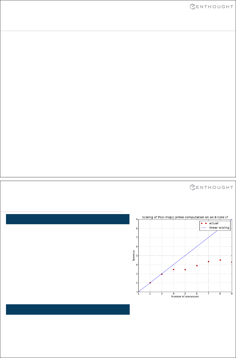
Task Pools
182
Pool() objects provide a convenient way to perform embarrassingly parallel
computations with automatic load balancing.
Pool(processes=None, initializer=None, initargs=())
processes – int, number of processes in pool, cpu_count() by default
initializer – callable, if not None, initializer(*initargs) is called by each
process when starting.
Methods:
map(func, iterable, chunksize=None) – parallel equivalent of the map()
builtin function. Blocks until result is ready and returns a list.
map_async(func, iterable, chunksize=None, callback=None)
Same as map(), nonblocking. Returns a result object.
imap(func, iterable, chunksize=None)
A version of map that returns an iterator instead of a list.
183
Task Pools
import multiprocessing as mp
def is_prime(num):
# determine whether num is prime
return (num, isp)
if __name__ == '__main__':
# create a pool with cpu_count() procs.
pl = mp.Pool()
results = pl.map(is_prime, range(50, 100))
for num, isp in results:
if isp: print num, “is prime”
BASIC POOL USAGE
$ python fermat_prime.py
53 is prime
59 is prime
61 is prime
67 is prime
...
OUTPUT Scaling computed for 106 integers while
varying pool size. Max speedup is ~4.5X
on 8 cores. This problem has high
communication overhead.
See demo_pool.py for the code.
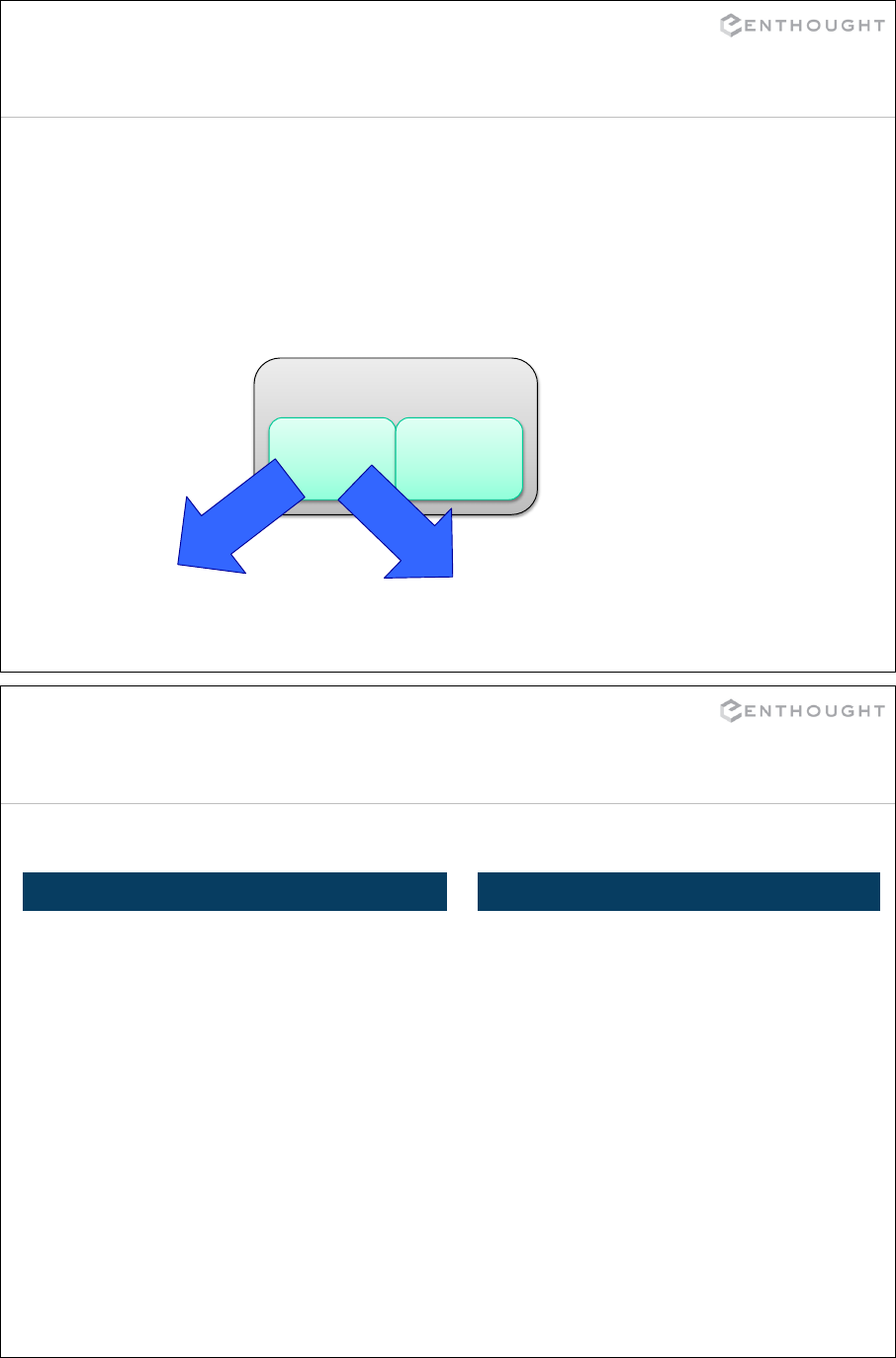
Shared Memory
184
Multiprocessing provides the Value and Array classes for shared memory
programming; there is also the multiprocessing.sharedctypes module to create
ctypes objects and arrays in shared memory.
Passing a shared memory object to the args of a Process() object will pass a proxy
to the target; the actual memory location is in shared memory (via mmap). Any
modifications to the proxy object will be seen by all processes.
This allows parallel array computations without much communication
overhead.
Shared Memory
a=Array() b=Value()
def worker1(a):
# modify a
def worker2(a):
# can see worker1’s changes
Multiprocessing + NumPy
185
NumPy arrays can be made to view multiprocessing shared memory objects.
import multiprocessing as mp
from multiprocessing import sharedctypes
from numpy import ctypeslib
def fill_arr(arr_view, i):
arr_view.fill(i)
if __name__ == '__main__':
ra = sharedctypes.RawArray('i', 4)
arr = ctypeslib.as_array(ra)
arr.shape = (2, 2)
p1 = mp.Process(target=fill_arr,
args=(arr[:1, :], 1))
p2 = mp.Process(target=fill_arr,
args=(arr[1:, :], 2))
p1.start(); p2.start()
p1.join(); p2.join()
print arr
SHARED MEMORY VIEW OUTPUT
$ python shared_numpy.py
[[1 1]
[2 2]]

186
Multiprocessing and others
The multiprocessing module is typically used for non-numerical calculations, when
Python’s role as a glue between several concurrent processes can be used.
For numerical calculations, numerically-optimized third-party libraries such as PyMPI,
MPI4Py, PyOpenCL, CLyther, PyCuda, etc. are typically used.
Multiprocessing is useful when one needs to add concurrency to an application
without requiring external dependencies.
187
NumPy

188
NumPy and SciPy
NDArray
multi-dimensional
array object
UFunc
fast array
math operations
fft random linalg
NumPy [ Data Structure Core ]
SciPy [ Scientific Algorithms ]
interpolate
integrate
spatial
weave
odr
stats
optimize
fftpack
sparse
special
linalg
signal
cluster
io
ndimage
189
NumPy
•Website: http://numpy.scipy.org/
•Offers Matlab-ish capabilities within Python
•NumPy replaces Numeric and Numarray
•Developed by Travis Oliphant
• >100 “committers” to the project (github.com)
•NumPy 1.0 released October, 2006
•NumPy 1.7.1 released April, 2013
•~45K downloads/month from SourceForge
This does not count:
•Linux distributions that include NumPy
•Enthought distributions that include NumPy
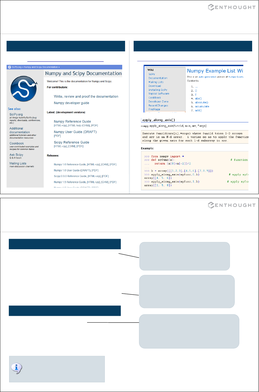
190
Helpful Sites
SCIPY DOCUMENTATION PAGE NUMPY EXAMPLES
http://docs.scipy.org/doc http://www.scipy.org/Numpy_Example_List_With_Doc
191
Getting Started
In [1]: from numpy import *
In [2]: __version__
Out[2]: 1.6.0
or
In [1]: from numpy import \
array, ...
C:\> ipython –-pylab
In [1]: array([1,2,3])
Out[1]: array([1, 2, 3])
IMPORT NUMPY
USING IPYTHON -PYLAB
Often at the command line, it is
handy to import everything from
NumPy into the command shell.
However, if you are writing scripts,
it is easier for others to read and
debug in the future if you use
explicit imports.
IPython has a ‘pylab’ mode where
it imports all of NumPy, Matplotlib,
and SciPy into the namespace for
you as a convenience. It also enables
threading for showing plots.
While IPython is used for all the
demos, ‘>>>’ is used on future
slides instead of ‘In [1]:’ to
save space.
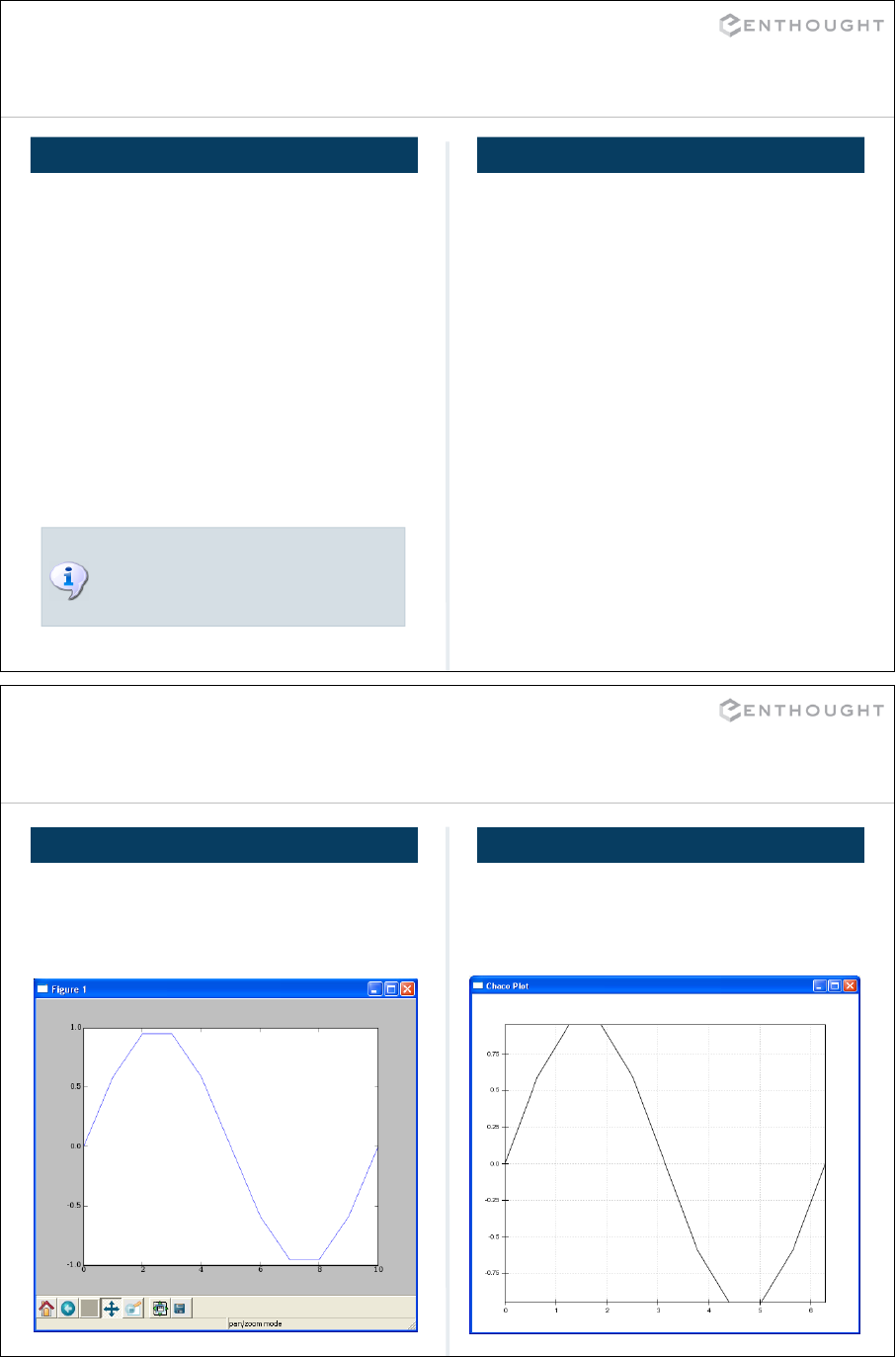
192
Array Operations
>>> a = array([1,2,3,4])
>>> b = array([2,3,4,5])
>>> a + b
array([3, 5, 7, 9])
>>> a * b
array([ 2, 6, 12, 20])
>>> a ** b
array([ 1, 8, 81, 1024])
# create array from 0 to 10
>>> x = arange(11.)
# multiply entire array by
# scalar value
>>> c = (2*pi)/10.
>>> c
0.62831853071795862
>>> c*x
array([ 0.,0.628,…,6.283])
# in-place operations
>>> x *= c
>>> x
array([ 0.,0.628,…,6.283])
# apply functions to array
>>> y = sin(x)
SIMPLE ARRAY MATH MATH FUNCTIONS
NumPy defines these constants:
pi = 3.14159265359
e = 2.71828182846
193
Plotting Arrays
>>> plot(x,y) >>> from chaco import shell
>>> shell.plot(x,y)
MATPLOTLIB CHACO SHELL
194
Matplotlib Basics
(an interlude)
195
http://matplotlib.org/
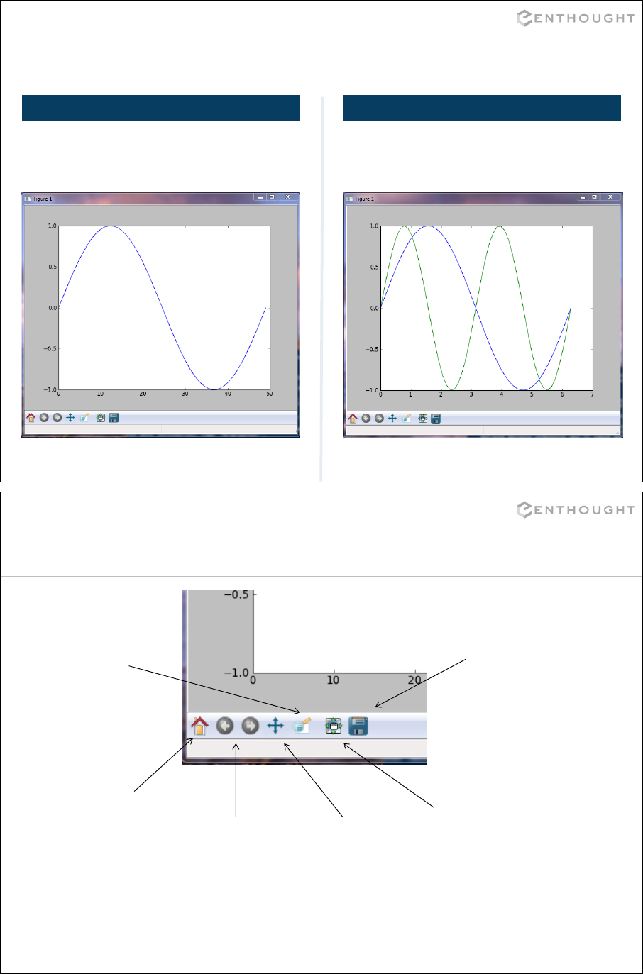
196
Line Plots
PLOT AGAINST INDICES MULTIPLE DATA SETS
>>> x = linspace(0,2*pi,50)
>>> plot(sin(x))
>>> plot(x, sin(x),
... x, sin(2*x))
Matplotlib Menu Bar
197
Zoom
tool Save to file
(png, svg,
eps, pdf, …)
Back to
original
view Previous/
next views Pan
tool
Plot size
parameter
within
window
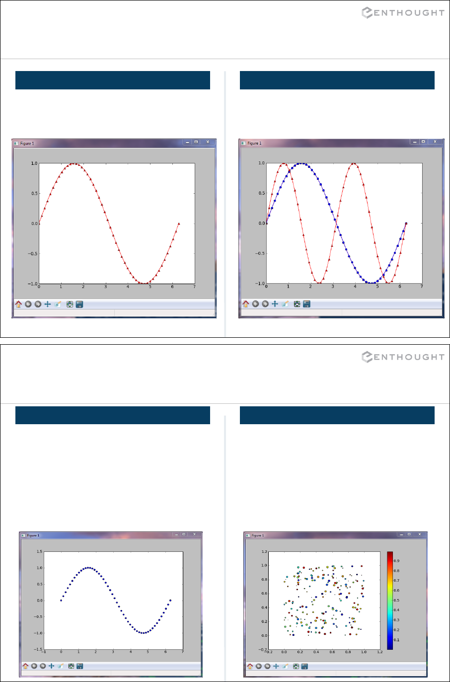
198
Line Plots
LINE FORMATTING MULTIPLE PLOT GROUPS
# red, dot-dash, triangles
>>> plot(x, sin(x), 'r-^')
>>> plot(x, sin(x), 'b-o',
... x, sin(2*x), 'r-^')
199
Scatter Plots
SIMPLE SCATTER PLOT COLORMAPPED SCATTER
>>> x = linspace(0,2*pi,50)
>>> y = sin(x)
>>> scatter(x, y)
# marker size/color set with data
>>> x = rand(200)
>>> y = rand(200)
>>> size = rand(200)*30
>>> color = rand(200)
>>> scatter(x, y, size, color)
>>> colorbar()
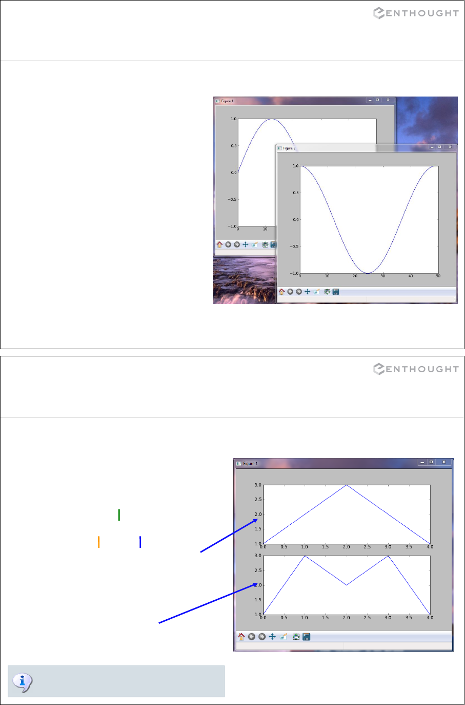
200
Multiple Figures
>>> t = linspace(0,2*pi,50)
>>> x = sin(t)
>>> y = cos(t)
# Now create a figure
>>> figure()
>>> plot(x)
# Now create a new figure.
>>> figure()
>>> plot(y)
201
Multiple Plots Using subplot
>>> x = array([1,2,3,2,1])
>>> y = array([1,3,2,3,1])
# To divide the plotting area
>>> subplot(2, 1, 1)
>>> plot(x)
# Now activate a new plot
# area.
>>> subplot(2, 1, 2)
>>> plot(y)
rows
columns
active plot
Plot 1
Plot 2
If this is used in a python script, a call
to the function show() is required.
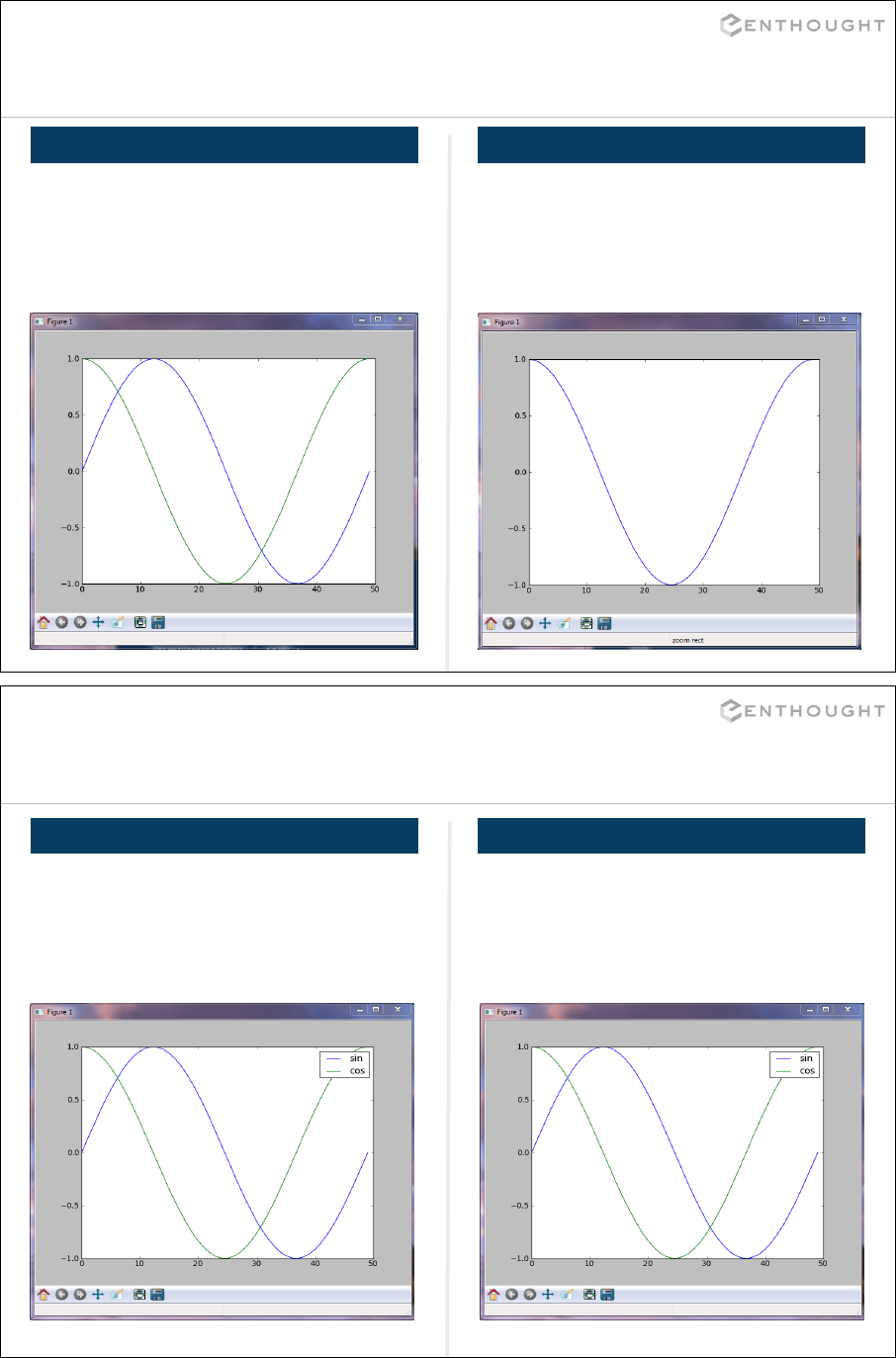
202
Adding Lines to a Plot
MULTIPLE PLOTS ERASING OLD PLOTS
# By default, previous lines
# are "held" on a plot.
>>> plot(sin(x))
>>> plot(cos(x))
# Set hold(False) to erase
# old lines
>>> plot(sin(x))
>>> hold(False)
>>> plot(cos(x))
203
Legend
LEGEND LABELS WITH PLOT LABELING WITH LEGEND
# Add labels in plot command.
>>> plot(sin(x), label='sin')
>>> plot(cos(x), label='cos')
>>> legend()
# Or as a list in legend().
>>> plot(sin(x))
>>> plot(cos(x))
>>> legend(['sin', 'cos'])
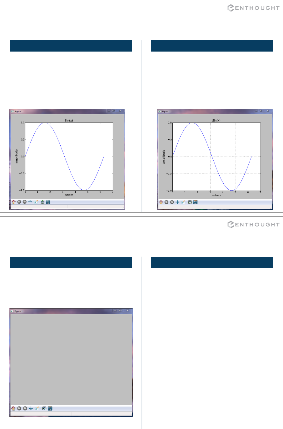
204
Titles and Grid
TITLES AND AXIS LABELS PLOT GRID
>>> plot(x, sin(x))
>>> xlabel('radians')
# Keywords set text properties.
>>> ylabel('amplitude',
... fontsize='large')
>>> title('Sin(x)')
# Display gridlines in plot
>>> grid()
205
Clearing and Closing Plots
CLEARING A FIGURE CLOSING PLOT WINDOWS
>>> plot(x, sin(x))
# clf will clear the current
# plot (figure).
>>> clf()
# close() will close the
# currently active plot window.
>>> close()
# close('all') closes all the
# plot windows.
>>> close('all')

206
Image Display
# Get the Lena image from scipy.
>>> from scipy.misc import lena
>>> img = lena()
# Display image with the jet
# colormap, and setting
# x and y extents of the plot.
>>> imshow(img,
... extent=[-25,25,-25,25],
... cmap = cm.bone)
# Add a colorbar to the display.
>>> colorbar()
207
Plotting from Scripts
INTERACTIVE MODE NON-INTERACTIVE MODE
# In IPython, plots show up
# as soon as a plot command
# is called.
>>> figure()
>>> plot(sin(x))
>>> figure()
>>> plot(cos(x))
# script.py
# In a script, you must call
# the show() command to display
# plots. Call it at the end of
# all your plot commands for
# best performance.
figure()
plot(sin(x))
figure()
plot(cos(x))
# Plots will not appear until
# this command is issued.
show()
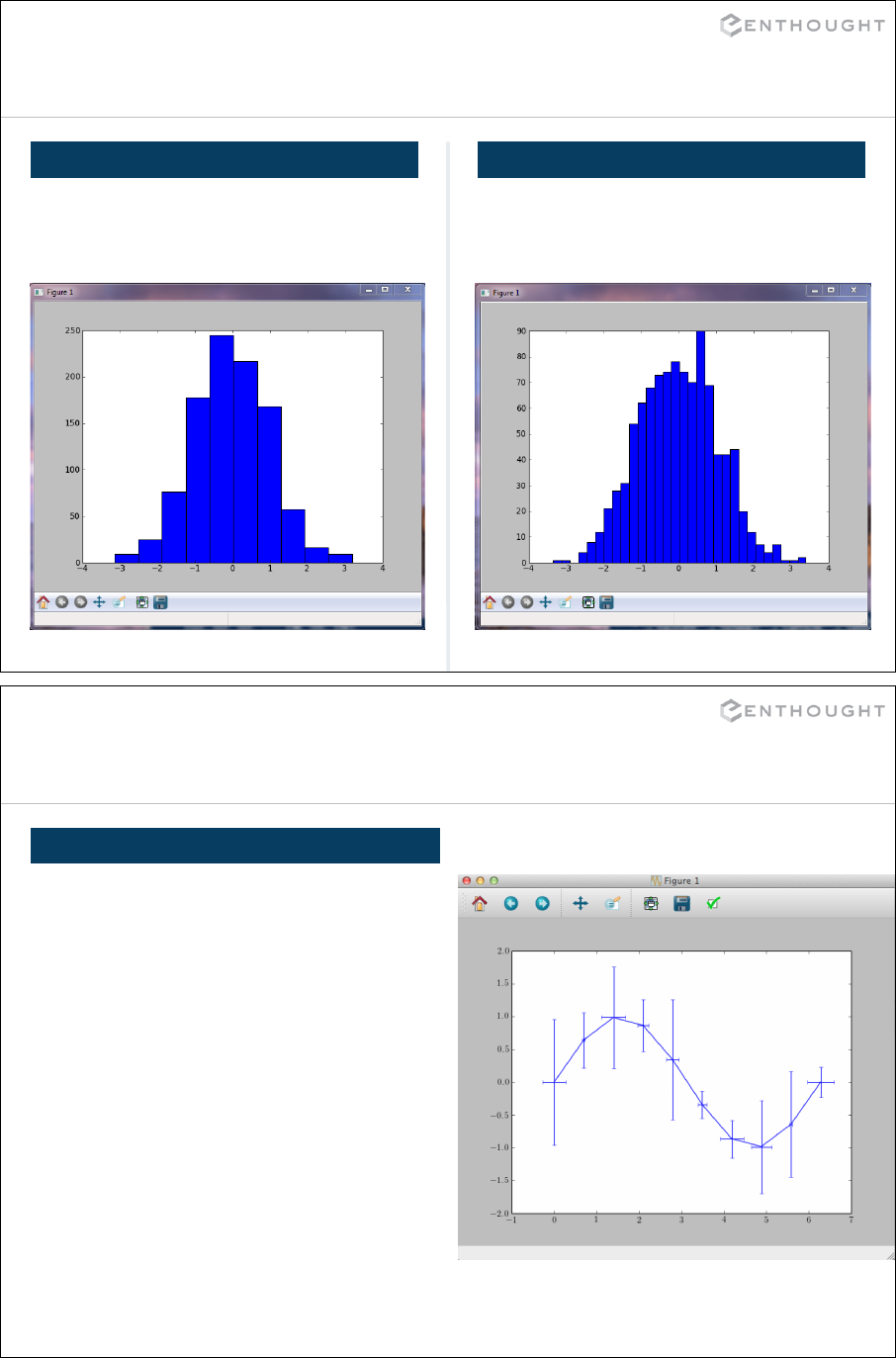
208
Histograms
HISTOGRAM HISTOGRAM 2
# plot histogram
# defaults to 10 bins
>>> hist(randn(1000))
# change the number of bins
>>> hist(randn(1000), 30)
209
Plots with error bars
ERRORBAR
# Assume points are known
# with errors in both axis
>>> x = linspace(0,2*pi,10)
>>> y = sin(x)
>>> yerr = rand(10)
>>> xerr = rand(10)/3
>>> errorbar(x, y, yerr, xerr)
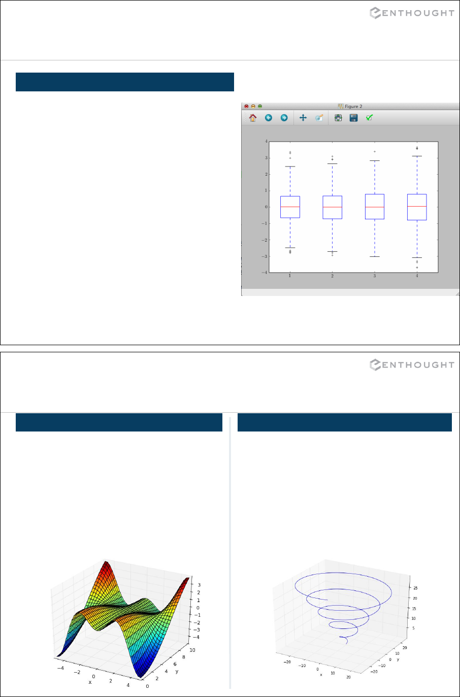
210
Plots with error bars II
BOXPLOT
# Assume 4 experiments have measured a
# quantity with a certain medians and
# std deviations.
# Data
>>> from numpy.random import normal
>>> exp = [normal(0, 1+i/5, size=(500,))
for i in np.arange(4.)]
>>> medians=[np.median(e) for e in exp]
>>> stds = [np.std(e) for e in exp]
# Plotting
>>> conf_intervals = [
(med - std, med + std) for
med, std in zip(medians, stds)]
>>> pos = np.arange(len(exp)))+1
>>> boxplot(exp, sym='k+',
positions=positions,
usermedians=medians,
conf_intervals=conf_intervals)
211
3D Plots with Matplotlib
SURFACE PLOT PARAMETRIC CURVE
>>> from mpl_toolkits.mplot3d import
Axes3D
>>> x, y = mgrid[-5:5:35j, 0:10:35j]
>>> z = x*sin(x)*cos(0.25*y)
>>> fig = figure()
>>> ax = fig.gca(projection='3d')
>>> ax.plot_surface(x, y, z,
... rstride=1, cstride=1,
... cmap=cm.jet)
>>> xlabel('x'); ylabel('y')
>>> from mpl_toolkits.mplot3d import
Axes3D
>>> t = linspace(0, 30, 1000)
>>> x, y, z = [t*cos(t), t*sin(t), t]
>>> fig = figure()
>>> ax = fig.gca(projection='3d')
>>> ax.plot(x, y, z)
>>> xlabel(‘x’)
>>> ylabel(‘y’)
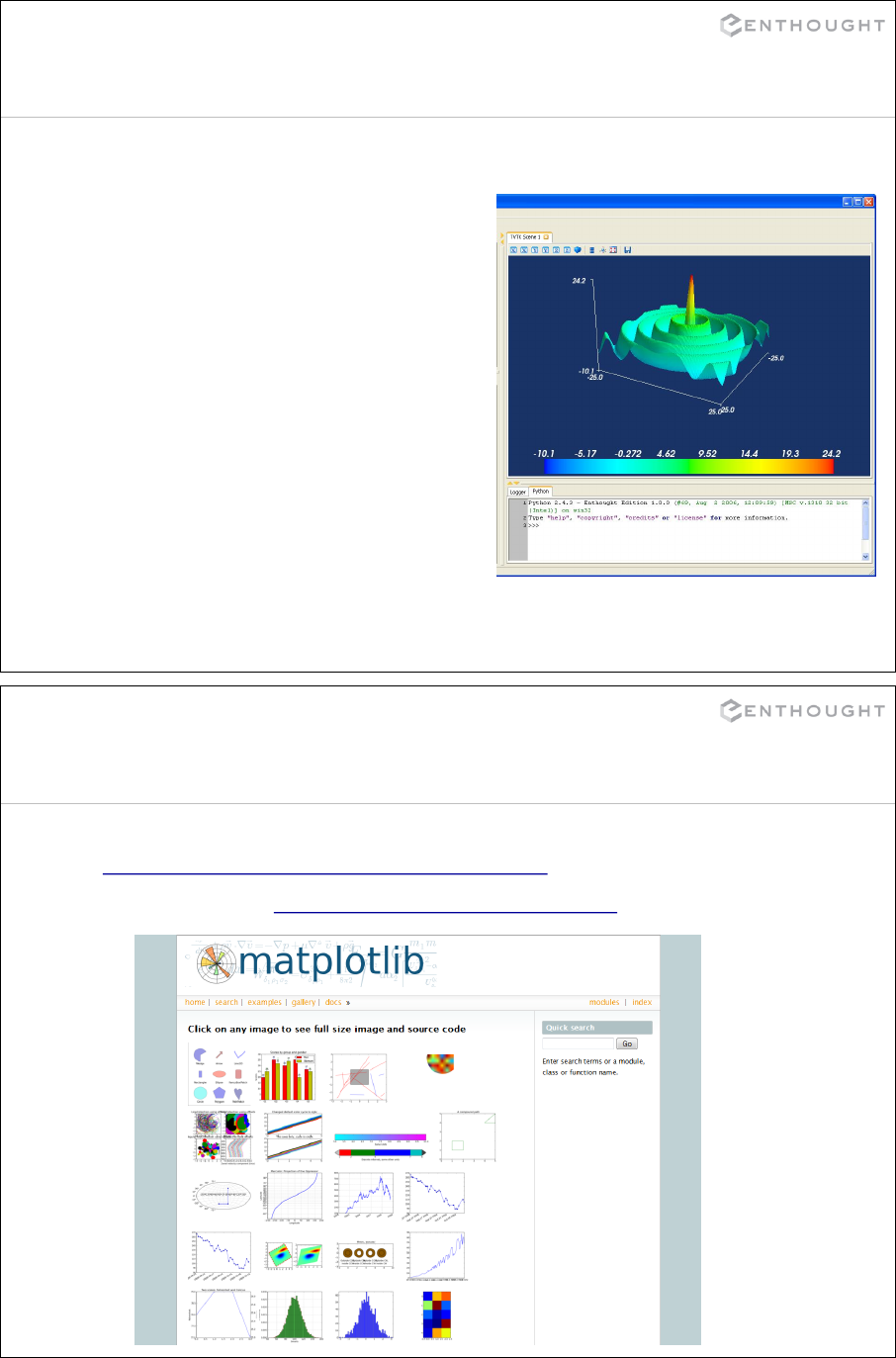
212
Surface Plots with mlab
# Create 2D array where values
# are radial distance from
# the center of array.
>>> from numpy import mgrid
>>> from scipy import special
>>> x,y = mgrid[-25:25:100j,
... -25:25:100j]
>>> r = sqrt(x**2+y**2)
# Calculate Bessel function of
# each point in array and scale.
>>> s = special.j0(r)*25
# Display surface plot.
>>> from mayavi import mlab
>>> mlab.surf(x,y,s)
>>> mlab.scalarbar()
>>> mlab.axes()
More Details
213
•Simple examples with increasing difficulty:
http://matplotlib.org/examples/index.html
•Gallery (huge): http://matplotlib.org/gallery.html

214
Continuing NumPy…
215
Introducing NumPy Arrays
>>> a = array([0,1,2,3])
>>> a
array([0, 1, 2, 3])
SIMPLE ARRAY CREATION
>>> type(a)
numpy.ndarray
CHECKING THE TYPE
>>> a.dtype
dtype('int32')
NUMERIC ‘TYPE’ OF ELEMENTS
>>> a.itemsize
4
BYTES PER ELEMENT
# Shape returns a tuple
# listing the length of the
# array along each dimension.
>>> a.shape
(4,)
>>> shape(a)
(4,)
# Size reports the entire
# number of elements in an
# array.
>>> a.size
4
>>> size(a)
4
ARRAY SHAPE
ARRAY SIZE

216
Introducing NumPy Arrays
# Return the number of bytes
# used by the data portion of
# the array.
>>> a.nbytes
16
BYTES OF MEMORY USED
>>> a.ndim
1
NUMBER OF DIMENSIONS
217
Setting Array Elements
>>> a.dtype
dtype('int32')
# assigning a float into
# an int32 array truncates
# the decimal part
>>> a[0] = 10.6
>>> a
array([10, 1, 2, 3])
# fill has the same behavior
>>> a.fill(-4.8)
>>> a
array([-4, -4, -4, -4])
BEWARE OF TYPE
COERCION
# set all values in an array
>>> a.fill(0)
>>> a
array([0, 0, 0, 0])
# this also works, but may
# be slower
>>> a[:] = 1
>>> a
array([1, 1, 1, 1])
FILL
>>> a[0]
0
>>> a[0] = 10
>>> a
array([10, 1, 2, 3])
ARRAY INDEXING

218
Slicing
# indices: 0 1 2 3 4
>>> a = array([10,11,12,13,14])
# [10,11,12,13,14]
>>> a[1:3]
array([11, 12])
# negative indices work also
>>> a[1:-2]
array([11, 12])
>>> a[-4:3]
array([11, 12])
SLICING ARRAYS
# omitted boundaries are
# assumed to be the beginning
# (or end) of the list
# grab first three elements
>>> a[:3]
array([10, 11, 12])
# grab last two elements
>>> a[-2:]
array([13, 14])
# every other element
>>> a[::2]
array([10, 12, 14])
var[lower:upper:step]
Extracts a portion of a sequence by specifying a lower and upper bound.
The lower-bound element is included, but the upper-bound element is not included.
Mathematically: [lower, upper). The step value specifies the stride between elements.
OMITTING INDICES
219
>>> a[1,3]
13
>>> a[1,3] = -1
>>> a
array([[ 0, 1, 2, 3],
[10,11,12,-1]])
Multi-Dimensional Arrays
>>> a = array([[ 0, 1, 2, 3],
[10,11,12,13]])
>>> a
array([[ 0, 1, 2, 3],
[10,11,12,13]])
>>> a[1]
array([10, 11, 12, -1])
row
column
MULTI-DIMENSIONAL ARRAYS
>>> a.shape
(2, 4)
SHAPE = (ROWS,COLUMNS)
GET/SET ELEMENTS
ADDRESS SECOND (ONETH)
ROW USING SINGLE INDEX
ELEMENT COUNT
>>> a.size
8
NUMBER OF DIMENSIONS
>>> a.ndim
2

220
Arrays from/to ASCII files
# Read data into a list of lists,
# and THEN convert to an array.
file = open('myfile.txt')
# Create a list for all the data.
data = []
for line in file:
# Read each row of data into a
# list of floats.
fields = line.split()
row_data = [float(x) for x
in fields]
# And add this row to the
# entire data set.
data.append(row_data)
# Finally, convert the "list of
# lists" into a 2D array.
data = array(data)
file.close()
BASIC PATTERN ARRAYS FROM/TO TXT FILES
# loadtxt() automatically generates
# an array from the txt file
arr = loadtxt('Data.txt', skiprows=1,
dtype=int, delimiter=",",
usecols = (0,1,2,4),
comments = "%")
# Save an array into a txt file
savetxt('filename', arr)
-- BEGINNING OF THE FILE
% Day, Month, Year, Skip, Avg Power
01, 01, 2000, x876, 13 % crazy day!
% we don’t have Jan 03rd
04, 01, 2000, xfed, 55
Data.txt
Arrays to/from Files
221
OTHER FILE FORMATS
Many file formats are supported in various packages:
File format Package name(s) Functions
txt numpy loadtxt, savetxt, genfromtxt, fromfile, tofile
csv csv reader, writer
Matlab scipy.io loadmat, savemat
hdf pytables, h5py
NetCDF netCDF4, scipy.io.netcdf netCDF4.Dataset, scipy.io.netcdf.netcdf_file
File format Package name Comments
wav scipy.io.wavfile Audio files
LAS/SEG-Y Scipy cookbook, EPD Data files in Geophysics
jpeg, png, … PIL, scipy.misc.pilutil Common image formats
FITS pyfits, astropy.io.fits Image files in Astronomy
This includes many industry specific formats:
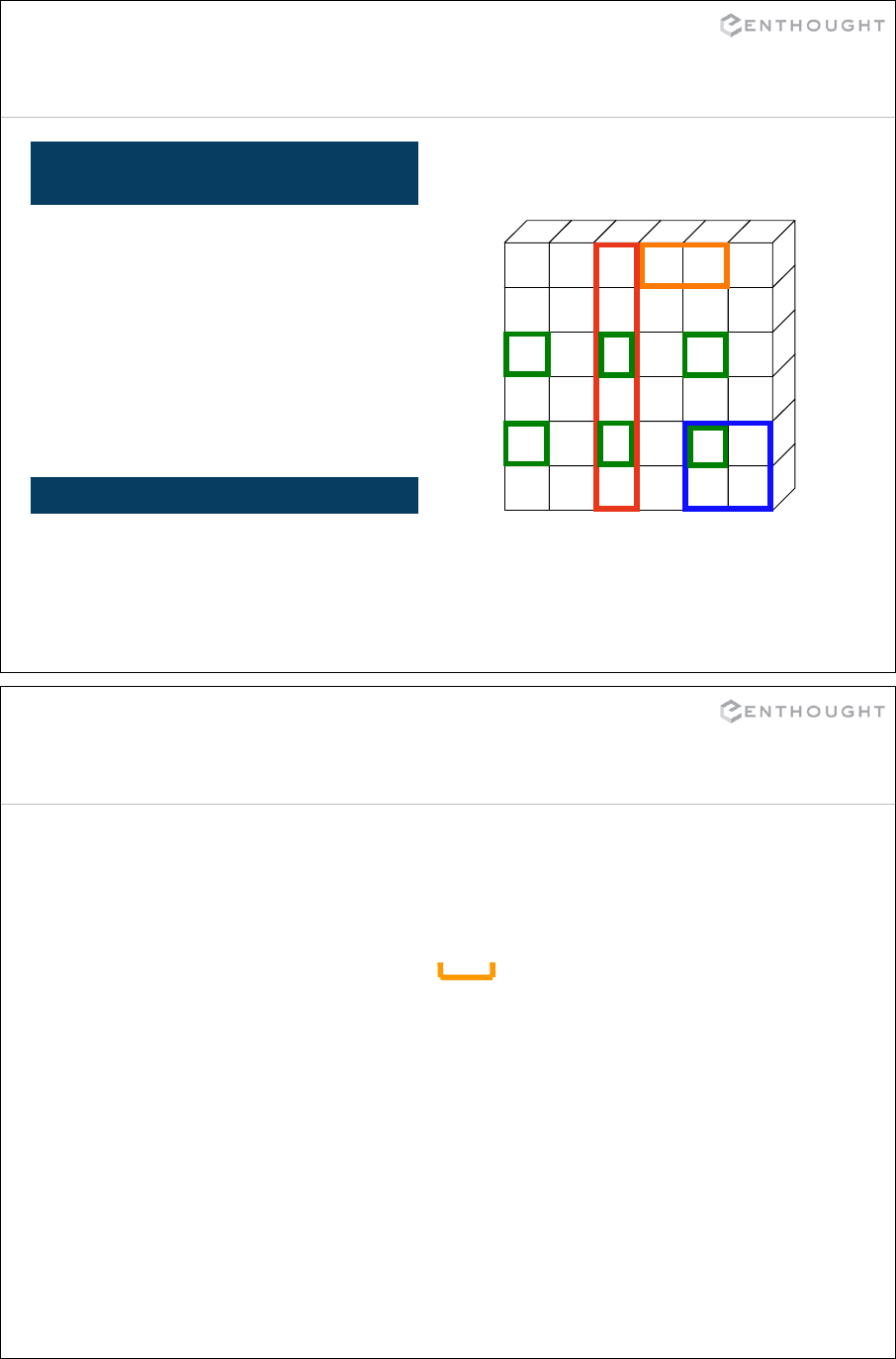
222
Array Slicing
>>> a[0,3:5]
array([3, 4])
>>> a[4:,4:]
array([[44, 45],
[54, 55]])
>>> a[:,2]
array([2,12,22,32,42,52])
50 51 52 53 54 55
40 41 42 43 44 45
30 31 32 33 34 35
20 21 22 23 24 25
10 11 12 13 14 15
0 1 2 3 4 5
SLICING WORKS MUCH LIKE
STANDARD PYTHON SLICING
>>> a[2::2,::2]
array([[20, 22, 24],
[40, 42, 44]])
STRIDES ARE ALSO POSSIBLE
223
Slices Are References
>>> a = array((0,1,2,3,4))
# create a slice containing only the
# last element of a
>>> b = a[2:4]
>>> b
array([2, 3])
>>> b[0] = 10
# changing b changed a!
>>> a
array([ 0, 1, 10, 3, 4])
Slices are references to memory in the original array.
Changing values in a slice also changes the original array.
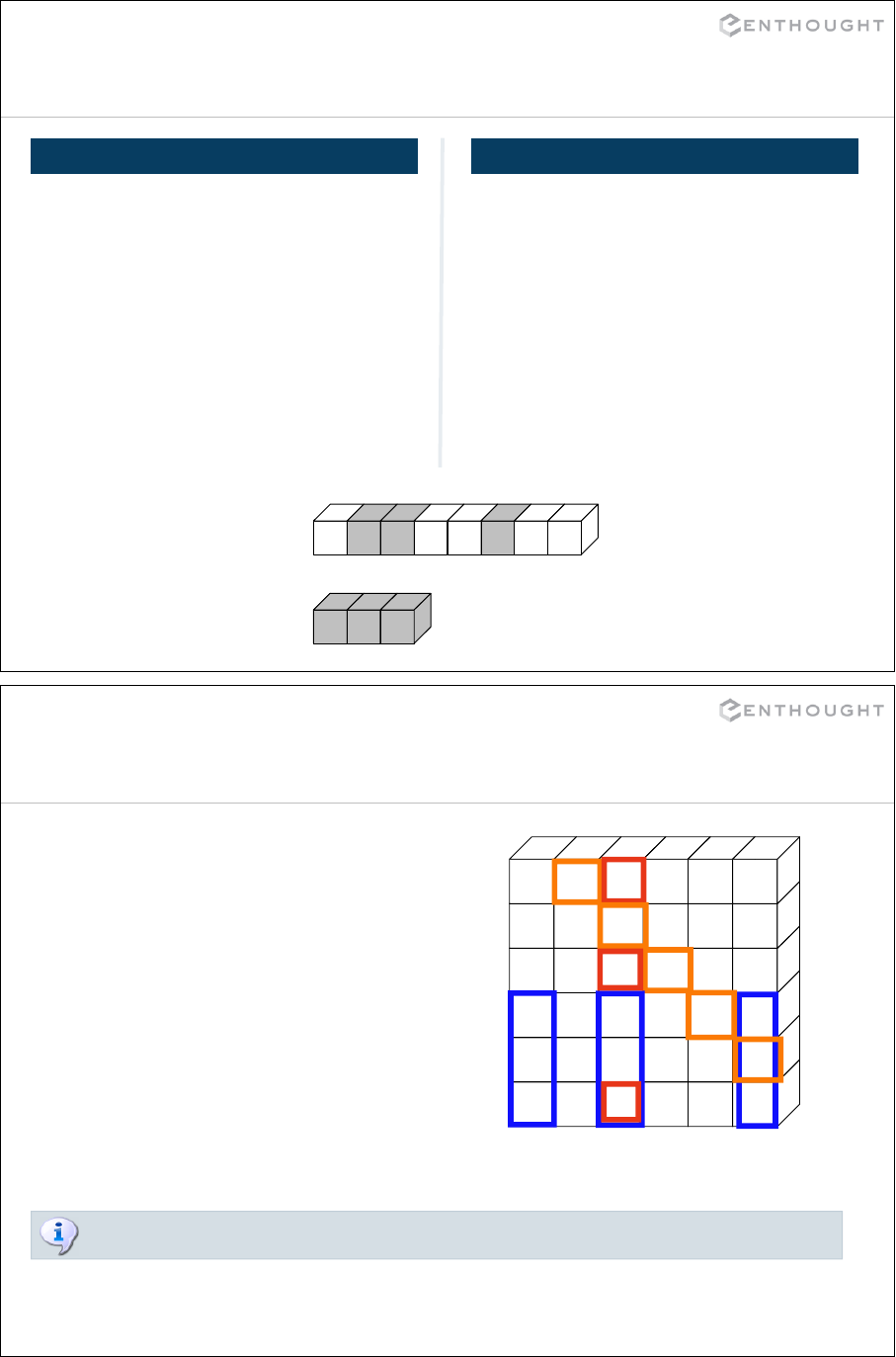
224
Fancy Indexing
# manual creation of masks
>>> mask = array([0,1,1,0,0,1,0,0],
... dtype=bool)
# conditional creation of masks
>>> mask2 = a < 30
# fancy indexing
>>> y = a[mask]
>>> print y
[10 20 50]
>>> a = arange(0,80,10)
# fancy indexing
>>> indices = [1, 2, -3]
>>> y = a[indices]
>>> print y
[10 20 50]
010 20 30 40 50 60 70
10 20 50
a
y
INDEXING BY POSITION INDEXING WITH BOOLEANS
225
Fancy Indexing in 2-D
>>> a[(0,1,2,3,4),(1,2,3,4,5)]
array([ 1, 12, 23, 34, 45])
>>> a[3:,[0, 2, 5]]
array([[30, 32, 35],
[40, 42, 45],
[50, 52, 55]])
>>> mask = array([1,0,1,0,0,1],
dtype=bool)
>>> a[mask,2]
array([2,22,52])
50 51 52 53 54 55
40 41 42 43 44 45
30 31 32 33 34 35
20 21 22 23 24 25
10 11 12 13 14 15
0 1 2 3 4 5
Unlike slicing, fancy indexing creates copies instead of a view into original array.
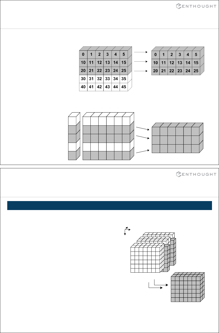
227
“Incomplete” Indexing
40 41 42 43 44 45
30 31 32 33 34 35
20 21 22 23 24 25
10 11 12 13 14 15
0 1 2 3 4 5
1
0
1
1
0
40 41 42 43 44 45
20 21 22 23 24 25
10 11 12 13 14 15
>>> y = a[condition]
condition a y
a y
>>> y = a[:3]
228
3D Example
# retrieve two slices from a
# 3D cube via indexing
>>> y = a[:,:,[2,-2]]
0
1
2
y
a
MULTIDIMENSIONAL
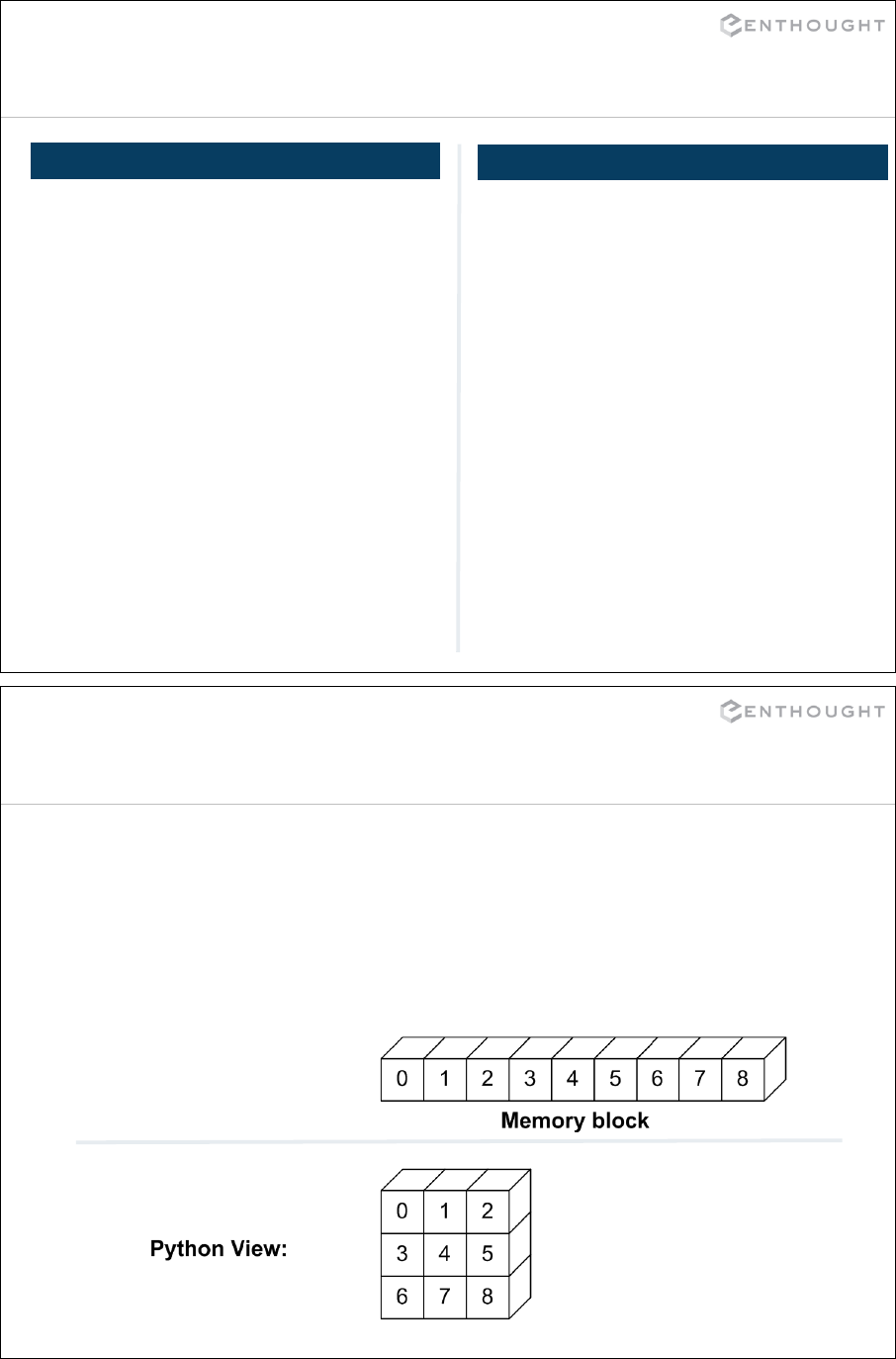
229
Where
# find the indices in array
# where expression is True
>>> a = array([0, 12, 5, 20])
>>> a > 10
array([False, True, False,
True], dtype=bool)
# Note: it returns a tuple!
>>> where(a > 10)
(array([1, 3]),)
1 DIMENSION
# In general, the tuple
# returned is the index of the
# element satisfying the
# condition in each dimension.
>>> a = array([[0, 12, 5, 20],
[1, 2, 11, 15]])
>>> loc = where(a > 10)
>>> loc
(array([0, 0, 1, 1]),
array([1, 3, 2, 3]))
# Result can be used in
# various ways:
>>> a[loc]
array([12, 20, 11, 15])
n DIMENSIONS
230
Array Data Structure
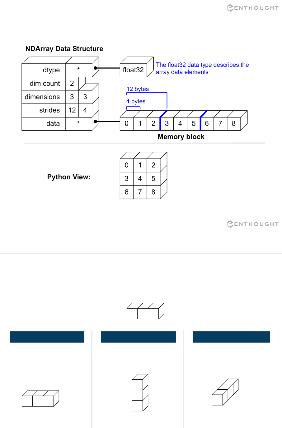
231
Array Data Structure
232
Indexing with newaxis
newaxis is a special index that inserts a new axis in the array at
the specified location.
Each newaxis increases the array’s dimensionality by 1.
>>> shape(a)
(3,)
>>> y = a[newaxis,:]
>>> shape(y)
(1, 3)
>>> y = a[:,newaxis]
>>> shape(y)
(3, 1)
> y = a[newaxis, newaxis, :]
> shape(y)
(1, 1, 3)
0 1 2
a
2
1
0
2
1
0
0 1 2
1 X 3 3 X 1 1 X 1 X 3

233
“Flattening” Arrays
a.flatten()
# Create a 2D array
>>> a = array([[0,1],
[2,3]])
# Flatten out elements to 1D
>>> b = a.flatten()
>>> b
array([0,1,2,3])
# Changing b does not change a
>>> b[0] = 10
>>> b
array([10,1,2,3])
>>> a
array([[0, 1],
[2, 3]])
a.flatten() converts a multi-
dimensional array into a 1-D array. The new
array is a copy of the original data.
a.flat
>>> a.flat
<numpy.flatiter obj...>
>>> a.flat[:]
array(0,1,2,3)
>>> b = a.flat
>>> b[0] = 10
>>> a
array([[10, 1],
[ 2, 3]])
no change
a.flat is an attribute that returns an
iterator object that accesses the data in the
multi-dimensional array data as a 1-D array.
It references the original memory.
changed!
234
“(Un)raveling” Arrays
a.ravel() a.ravel() MAKES A COPY
# create a 2-D array
>>> a = array([[0,1],
[2,3]])
# flatten out elements to 1-D
>>> b = a.ravel()
>>> b
array([0,1,2,3])
# changing b does change a
>>> b[0] = 10
>>> b
array([10,1,2,3])
>>> a
array([[10, 1],
[ 2, 3]])
changed!
a.ravel() is the same as a.flatten(),
but returns a reference (or view) of the array
if possible (i.e., the memory is contiguous).
Otherwise the new array copies the data.
# create a 2-D array
>>> a = array([[0,1],
[2,3]])
# transpose array so memory
# layout is no longer contiguous
>>> aa = a.transpose()
>>> aa
array([[0, 2],
[1, 3]])
# ravel creates a copy of data
>>> b = aa.ravel()
array([0,2,1,3])
# changing b doesn't change a
>>> b[0] = 10
>>> b
array([10,1,2,3])
>>> a
array([[0, 1],
[2, 3]])

235
Reshaping Arrays
>>> a = arange(6)
>>> a
array([0, 1, 2, 3, 4, 5])
>>> a.shape
(6,)
# reshape array in-place to
# 2x3
>>> a.shape = (2,3)
>>> a
array([[0, 1, 2],
[3, 4, 5]])
SHAPE
# return a new array with a
# different shape
>>> a.reshape(3,2)
array([[0, 1],
[2, 3],
[4, 5]])
# reshape cannot change the
# number of elements in an
# array
>>> a.reshape(4,2)
ValueError: total size of new
array must be unchanged
RESHAPE
236
Transpose
>>> a = array([[0,1,2],
... [3,4,5]])
>>> a.shape
(2,3)
# Transpose swaps the order
# of axes. For 2-D this
# swaps rows and columns.
>>> a.transpose()
array([[0, 3],
[1, 4],
[2, 5]])
# The .T attribute is
# equivalent to transpose().
>>> a.T
array([[0, 3],
[1, 4],
[2, 5]])
TRANSPOSE
>>> b = a.T
# Changes to b alter a.
>>> b[0,1] = 30
>>> a
array([[ 0, 1, 2],
[30, 4, 5]])
# Transpose does not move
# values around in memory. It
# only changes the order of
# "strides" in the array
>>> a.strides
(12, 4)
>>> a.T.strides
(4, 12)
TRANSPOSE RETURNS VIEWS
TRANSPOSE AND STRIDES

237
Squeeze
>>> a = array([[1,2,3],
... [4,5,6]])
>>> a.shape
(2,3)
# insert an "extra" dimension
>>> a.shape = (2,1,3)
>>> a
array([[[0, 1, 2]],
[[3, 4, 5]]])
# squeeze removes any
# dimension with length==1
>>> a = a.squeeze()
>>> a.shape
(2,3)
SQUEEZE
238
Diagonals
>>> a = array([[11,21,31],
... [12,22,32],
... [13,23,33]])
# Extract the diagonal from
# an array.
>>> a.diagonal()
array([11, 22, 33])
# Use offset to move off the
# main diagonal (offset can
# be negative).
>>> a.diagonal(offset=1)
array([21, 32])
DIAGONAL DIAGONALS WITH INDEXING
# "Fancy" indexing also works.
>>> i = [0,1,2]
>>> a[i, i]
array([11, 22, 33])
# Indexing can also be used
# to set diagonal values…
>>> a[i, i] = 2
>>> i2 = array([0,1])
# upper diagonal
>>> a[i2, i2+1] = 1
# lower diagonal
>>> a[i2+1, i2]= -1
>>> a
array([[ 2, 1, 31],
[-1, 2, 1],
[13, -1, 2]])

239
Complex Numbers
>>> a = array([1+1j, 2, 3, 4])
array([1.+1.j, 2.+0.j, 3.+0.j,
4.+0.j])
>>> a.dtype
dtype('complex128')
# real and imaginary parts
>>> a.real
array([ 1., 2., 3., 4.])
>>> a.imag
array([ 1., 0., 0., 0.])
# set imaginary part to a
# different set of values
>>> a.imag = (1,2,3,4)
>>> a
array([1.+1.j, 2.+2.j, 3.+3.j,
4.+4.j])
COMPLEX ARRAY ATTRIBUTES
>>> a = array([0., 1, 2, 3])
# .real and .imag attributes
# are available
>>> a.real
array([ 0., 1., 2., 3.])
>>> a.imag
array([ 0., 0., 0., 0.])
# but .imag is read-only
>>> a.imag = (1,2,3,4)
TypeError: array does not
have imaginary part to set
FLOAT (AND OTHER) ARRAYS
>>> a.conj()
array([1.-1.j, 2.-2.j, 3.-3.j,
4.-4.j])
CONJUGATION
240
Array Constructor Examples
# Default to double precision
>>> a = array([0,1.0,2,3])
>>> a.dtype
dtype('float64')
>>> a.nbytes
32
FLOATING POINT ARRAYS
>>> a = array([0,1.,2,3],
... dtype=float32)
>>> a.dtype
dtype('float32')
>>> a.nbytes
16
REDUCING PRECISION
>>> a = array([0,1,2,3],
... dtype=uint8)
>>> a.dtype
dtype('uint8')
>>> a.nbytes
4
UNSIGNED INTEGER BYTE
ARRAY FROM BINARY DATA
# frombuffer or fromfile
# to create an array from
# binary data.
>>> a = frombuffer('foo',
... dtype=uint8)
>>> a
array([102, 111, 111])
# Reverse operation
>>> a.tofile('foo.dat')

241
NumPy dtypes
Basic Type Available NumPy types Comments
Boolean bool Elements are 1 byte in size.
Integer int8, int16, int32, int64,
int128, int
int defaults to the size of long in C for the
platform.
Unsigned
Integer uint8, uint16, uint32, uint64,
uint128, uint
uint defaults to the size of unsigned long in
C for the platform.
Float float16, float32, float64,
float,longfloat,
float is always a double precision floating
point value (64 bits). longfloat represents
large precision floats. Its size is platform
dependent.
Complex complex64, complex128,
complex, longcomplex
The real and imaginary elements of a
complex64 are each represented by a single
precision (32 bit) value for a total size of 64
bits.
Strings str, unicode For example, dtype=‘S4’ would be used for an
array of 4-character strings.
Object object Represent items in array as Python objects.
Records void Used for arbitrary data structures.
242
Type Casting
>>> a = array([1.5, -3],
... dtype=float32)
>>> a
array([ 1.5, -3.], dtype=float32)
# upcast
>>> asarray(a, dtype=float64)
array([ 1.5, -3. ])
# downcast
>>> asarray(a, dtype=uint8)
array([ 1, 253], dtype=uint8)
# asarray is efficient.
# It does not make a copy if the
# type is the same.
>>> b = asarray(a, dtype=float32)
>>> b[0] = 2.0
>>> a
array([ 2., -3.],dtype=float32)
>>> a = array([1.5, -3],
... dtype=float64)
>>> a.astype(float32)
array([ 1.5, -3.], dtype=float32)
>>> a.astype(uint8)
array([ 1, 253],dtype=uint8)
# astype is safe.
# It always returns a copy of
# the array.
>>> b = a.astype(float64)
>>> b[0] = 2.0
>>> a
array([1.5, -3.])
ASARRAY ASTYPE

243
Array Calculation Methods
>>> a = array([[1,2,3],
[4,5,6]])
# sum() defaults to adding up
# all the values in an array.
>>> sum(a)
21
# supply the keyword axis to
# sum along the 0th axis
>>> sum(a, axis=0)
array([5, 7, 9])
# supply the keyword axis to
# sum along the last axis
>>> sum(a, axis=-1)
array([ 6, 15])
SUM FUNCTION
# a.sum() defaults to adding
# up all values in an array.
>>> a.sum()
21
# supply an axis argument to
# sum along a specific axis
>>> a.sum(axis=0)
array([5, 7, 9])
SUM ARRAY METHOD
# product along columns
>>> a.prod(axis=0)
array([ 4, 10, 18])
# functional form
>>> prod(a, axis=0)
array([ 4, 10, 18])
PRODUCT
244
Min/Max
# Find index of minimum value.
>>> a.argmin(axis=0)
2
# functional form
>>> argmin(a, axis=0)
2
ARGMIN
MIN
>>> a = array([2.,3.,0.,1.])
>>> a.min(axis=0)
0.0
# Use NumPy's amin() instead
# of Python's built-in min()
# for speedy operations on
# multi-dimensional arrays.
>>> amin(a, axis=0)
0.0
# Find index of maximum value.
>>> a.argmax(axis=0)
1
# functional form
>>> argmax(a, axis=0)
1
ARGMAX
MAX
>>> a = array([2.,3.,0.,1.])
>>> a.max(axis=0)
3.0
# functional form
>>> amax(a, axis=0)
3.0

245
Statistics Array Methods
>>> a = array([[1,2,3],
[4,5,6]])
# mean value of each column
>>> a.mean(axis=0)
array([ 2.5, 3.5, 4.5])
>>> mean(a, axis=0)
array([ 2.5, 3.5, 4.5])
>>> average(a, axis=0)
array([ 2.5, 3.5, 4.5])
# average can also calculate
# a weighted average
>>> average(a, weights=[1,2],
... axis=0)
array([ 3., 4., 5.])
MEAN
# Standard Deviation
>>> a.std(axis=0)
array([ 1.5, 1.5, 1.5])
# variance
>>> a.var(axis=0)
array([2.25, 2.25, 2.25])
>>> var(a, axis=0)
array([2.25, 2.25, 2.25])
STANDARD DEV./VARIANCE
246
Other Array Methods
# Limit values to a range.
>>> a = array([[1,2,3],
[4,5,6]])
# Set values < 3 equal to 3.
# Set values > 5 equal to 5.
>>> a.clip(3, 5)
array([[3, 3, 3],
[4, 5, 5]])
CLIP
# Round values in an array.
# NumPy rounds to even, so
# 1.5 and 2.5 both round to 2.
>>> a = array([1.35, 2.5, 1.5])
>>> a.round()
array([ 1., 2., 2.])
# Round to first decimal place.
>>> a.round(decimals=1)
array([ 1.4, 2.5, 1.5])
ROUND
# Calculate max – min for
# array along columns
>>> a.ptp(axis=0)
array([3, 3, 3])
# max – min for entire array.
>>> a.ptp(axis=None)
5
PEAK TO PEAK

247
Summary of (most) array
attributes/methods (1/4)
BASIC ATTRIBUTES
a.dtype Numerical type of array elements: float 32, uint8, etc.
a.shape Shape of array (m, n, o, …)
a.size Number of elements in entire array
a.itemsize Number of bytes used by a single element in the array
a.nbytes Number of bytes used by entire array (data only)
a.ndim Number of dimensions in the array
SHAPE OPERATIONS
a.flat An iterator to step through array as if it were 1D
a.flatten() Returns a 1D copy of a multi-dimensional array
a.ravel() Same as flatten(), but returns a "view" if possible
a.resize(new_size) Changes the size/shape of an array in place
a.swapaxes(axis1, axis2) Swaps the order of two axes in an array
a.transpose(*axes) Swaps the order of any number of array axes
a.T Shorthand for a.transpose()
a.squeeze() Removes any length==1 dimensions from an array
248
Summary of (most) array
attributes/methods (2/4)
FILL AND COPY
a.copy() Returns a copy of the array
a.fill(value) Fills an array with a scalar value
CONVERSION/COERCION
a.tolist() Converts array into nested lists of values
a.tostring() Raw copy of array memory into a Python string
a.astype(dtype) Returns array coerced to the given type
a.byteswap(False) Converts byte order (big <->little endian)
a.view(type_or_dtype) Creates a new ndarray that sees the same memory but interprets it as a
new datatype (or subclass of ndarray)
COMPLEX NUMBERS
a.real Returns the real part of the array
a.imag Returns the imaginary part of the array
a.conjugate() Returns the complex conjugate of the array
a.conj() Returns the complex conjugate of the array (same as conjugate)

249
Summary of (most) array
attributes/methods (3/4)
SAVING
a.dump(file) Stores binary array data to file
a.dumps() Returns a binary pickle of the data as a string
a.tofile(fid, sep="",
format="%s") Formatted ASCII output to a file
SEARCH/SORT
a.nonzero() Returns indices for all non-zero elements in the array
a.sort(axis=-1) Sort the array elements in place, along axis
a.argsort(axis=-1) Finds indices for sorted elements, along axis
a.searchsorted(b) Finds indices where elements of b would be inserted in a to maintain order
ELEMENT MATH OPERATIONS
a.clip(low, high) Limits values in the array to the specified range
a.round(decimals=0) Rounds to the specified number of digits
a.cumsum(axis=None) Cumulative sum of elements along axis
a.cumprod(axis=None) Cumulative product of elements along axis
250
Summary of (most) array
attributes/methods (4/4)
All the following methods “reduce” the size of the array by 1 dimension by
carrying out an operation along the specified axis. If axis is None, the
operation is carried out across the entire array.
REDUCTION METHODS
a.sum(axis=None) Sums values along axis
a.prod(axis=None) Finds the product of all values along axis
a.min(axis=None) Finds the minimum value along axis
a.max(axis=None) Finds the maximum value along axis
a.argmin(axis=None) Finds the index of the minimum value along axis
a.argmax(axis=None) Finds the index of the maximum value along axis
a.ptp(axis=None) Calculates a.max(axis) – a.min(axis)
a.mean(axis=None) Finds the mean (average) value along axis
a.std(axis=None) Finds the standard deviation along axis
a.var(axis=None) Finds the variance along axis
a.any(axis=None) True if any value along axis is non-zero (logical OR)
a.all(axis=None) True if all values along axis are non-zero (logical AND)

251
Array Creation Functions
arange(start,stop=None,step=1,
dtype=None)
Nearly identical to Python’s range().
Creates an array of values in the range
[start,stop) with the specified step value.
Allows non-integer values for start, stop, and
step. Default dtype is derived from the start,
stop, and step values.
>>> arange(4)
array([0, 1, 2, 3])
>>> arange(0, 2*pi, pi/4)
array([ 0.000, 0.785, 1.571,
2.356, 3.142, 3.927, 4.712,
5.497])
# Be careful…
>>> arange(1.5, 2.1, 0.3)
array([ 1.5, 1.8, 2.1])
ARANGE ONES, ZEROS
ones(shape, dtype=float64)
zeros(shape, dtype=float64)
shape is a number or sequence specifying
the dimensions of the array. If dtype is not
specified, it defaults to float64.
>>> ones((2,3),dtype=float32)
array([[ 1., 1., 1.],
[ 1., 1., 1.]],
dtype=float32)
>>> zeros(3)
array([ 0., 0., 0.])
252
Array Creation Functions (cont.)
# Generate an n by n identity
# array. The default dtype is
# float64.
>>> a = identity(4)
>>> a
array([[ 1., 0., 0., 0.],
[ 0., 1., 0., 0.],
[ 0., 0., 1., 0.],
[ 0., 0., 0., 1.]])
>>> a.dtype
dtype('float64')
>>> identity(4, dtype=int)
array([[ 1, 0, 0, 0],
[ 0, 1, 0, 0],
[ 0, 0, 1, 0],
[ 0, 0, 0, 1]])
EMPTY AND FILL
IDENTITY
# empty(shape, dtype=float64,
# order='C')
>>> a = empty(2)
>>> a
array([1.78021120e-306,
6.95357225e-308])
# fill array with 5.0
>>> a.fill(5.0)
array([5., 5.])
# alternative approach
# (slightly slower)
>>> a[:] = 4.0
array([4., 4.])

253
Array Creation Functions (cont.)
# Generate N evenly spaced
# elements between (and
# including) start and
# stop values.
>>> linspace(0,1,5)
array([0.,0.25.,0.5,0.75, 1.0])
ROW SHORTCUT
LINSPACE
# r_ and c_ are "handy" tools
# (cough hacks…) for creating
# row and column arrays.
# used like arange
# -- real stride value
>>> r_[0:1:.25]
array([ 0., 0.25., 0.5, 0.75])
# used like linspace
# -- complex stride value
>>> r_[0:1:5j]
array([0.,0.25.,0.5,0.75,1.0])
# concatenate elements
>>> r_[(1,2,3),0,0,(4,5)]
array([1, 2, 3, 0, 0, 4, 5])
LOGSPACE
# Generate N evenly spaced
# elements on a log scale
# between base**start and
# base**stop (default base=10).
>>> logspace(0,1,5)
array([ 1., 1.77, 3.16, 5.62,
10.])
254
Array Creation Functions (cont.)
OGRID
MGRID
# Construct an "open" grid
# of points (not filled in
# but correctly shaped for
# math operations to be
# broadcast correctly).
>>> x,y = ogrid[0:3,0:3]
>>> x
array([[0],
[1],
[2]])
>>> y
array([[0, 1, 2]])
>>> print x+y
[[0 1 2]
[1 2 3]
[2 3 4]]
# Get equally spaced points
# in N output arrays for an
# N-dimensional (mesh) grid.
>>> x,y = mgrid[0:5,0:5]
>>> x
array([[0, 0, 0, 0, 0],
[1, 1, 1, 1, 1],
[2, 2, 2, 2, 2],
[3, 3, 3, 3, 3],
[4, 4, 4, 4, 4]])
>>> y
array([[0, 1, 2, 3, 4],
[0, 1, 2, 3, 4],
[0, 1, 2, 3, 4],
[0, 1, 2, 3, 4],
[0, 1, 2, 3, 4]])

255
Matrix Objects
# Matlab-like creation from string
>>> A = mat('1,2,4;2,5,3;7,8,9')
>>> print A
Matrix([[1, 2, 4],
[2, 5, 3],
[7, 8, 9]])
# matrix exponents
>>> print A**4
Matrix([[ 6497, 9580, 9836],
[ 7138, 10561, 10818],
[18434, 27220, 27945]])
# matrix multiplication
>>> print A*A.I
Matrix([[ 1., 0., 0.],
[ 0., 1., 0.],
[ 0., 0., 1.]])
BLOCK MATRICES
MATRIX CREATION
# create a matrix from
# sub-matrices
>>> a = array([[1,2],
[3,4]])
>>> b = array([[10,20],
[30,40]])
>>> bmat('a,b;b,a')
matrix([[ 1, 2, 10, 20],
[ 3, 4, 30, 40],
[10, 20, 1, 2],
[30, 40, 3, 4]])
256
Element by element distance
calculation using
Trig and Other Functions
sin(x) sinh(x)
cos(x) cosh(x)
arccos(x) arccosh(x)
arctan(x) arctanh(x)
arcsin(x) arcsinh(x)
arctan2(x,y)
22 yx
TRIGONOMETRIC
exp(x) log(x)
log10(x) sqrt(x)
absolute(x) conjugate(x)
negative(x) ceil(x)
floor(x) fabs(x)
hypot(x,y) fmod(x,y)
maximum(x,y) minimum(x,y)
OTHERS
hypot(x,y)
VECTOR OPERATIONS
dot(x,y) vdot(x,y)
inner(x,y) outer(x,y)
cross(x,y) kron(x,y)
tensordot(x,y[,axis])
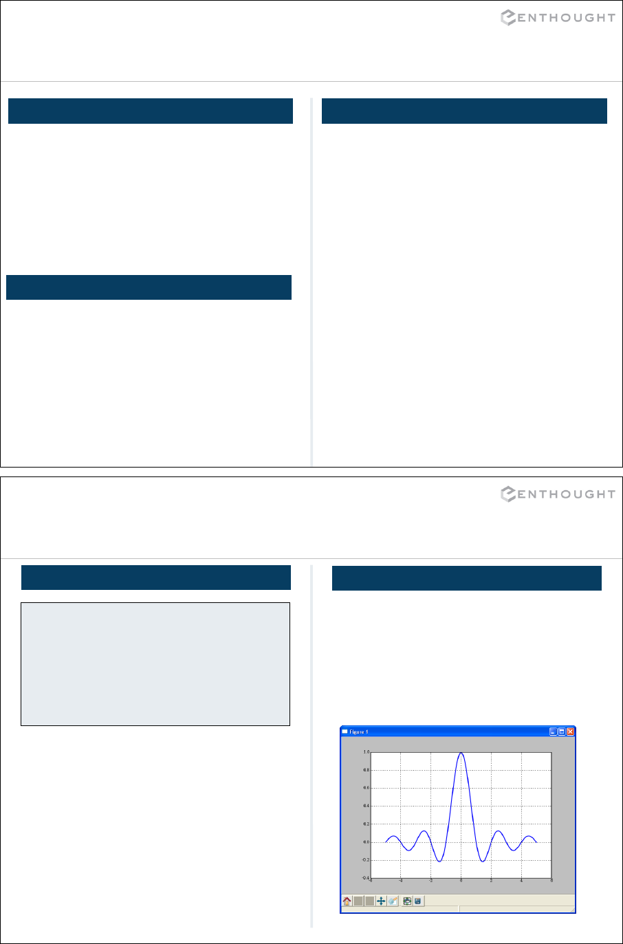
257
More Basic Functions
TYPE HANDLING
iscomplexobj
iscomplex
isrealobj
isreal
imag
real
real_if_close
isscalar
isneginf
isposinf
isinf
isfinite
isnan
nan_to_num
common_type
typename
SHAPE MANIPULATION
atleast_1d
atleast_2d
atleast_3d
expand_dims
apply_over_axes
apply_along_axis
hstack
vstack
dstack
column_stack
hsplit
vsplit
dsplit
split
squeeze
OTHER USEFUL FUNCTIONS
fix
mod
amax
amin
ptp
sum
cumsum
prod
cumprod
diff
angle
roots
poly
any
all
disp
unique
nansum
nanmax
nanargmax
nanargmin
nanmin
unwrap
sort_complex
trim_zeros
fliplr
flipud
rot90
eye
diag
select
extract
insert
258
Vectorizing Functions
# special.sinc already available
# This is just for show.
def sinc(x):
if x == 0.0:
return 1.0
else:
w = pi*x
return sin(w) / w
# attempt
>>> x = array((1.3, 1.5))
>>> sinc(x)
ValueError: The truth value of
an array with more than one
element is ambiguous. Use
a.any() or a.all()
>>> from numpy import vectorize
>>> vsinc = vectorize(sinc)
>>> vsinc(x)
array([-0.1981, -0.2122])
>>> x2 = linspace(-5, 5, 101)
>>> plot(x2, vsinc(x2))
SOLUTION
SCALAR SINC FUNCTION

259
Mathematical Binary Operators
a + b add(a,b)
a - b subtract(a,b)
a % b remainder(a,b)
a * b multiply(a,b)
a / b divide(a,b)
a ** b power(a,b)
MULTIPLY BY A SCALAR
ELEMENT BY ELEMENT
ADDITION
ADDITION USING AN OPERATOR
FUNCTION
>>> a = array((1,2))
>>> a*3.
array([3., 6.])
>>> a = array([1,2])
>>> b = array([3,4])
>>> a + b
array([4, 6])
>>> add(a,b)
array([4, 6])
# Overwrite contents of a.
# Saves array creation
# overhead.
>>> add(a,b,a) # a += b
array([4, 6])
>>> a
array([4, 6])
IN-PLACE OPERATION
260
Comparison and Logical Operators
>>> a = array(((1,2,3,4),(2,3,4,5)))
>>> b = array(((1,2,5,4),(1,3,4,5)))
>>> a == b
array([[True, True, False, True],
[False, True, True, True]])
# functional equivalent
>>> equal(a,b)
array([[True, True, False, True],
[False, True, True, True]])
equal (==)
greater_equal (>=)
logical_and
logical_not
not_equal (!=)
less (<)
logical_or
greater (>)
less_equal (<=)
logical_xor
2-D EXAMPLE Be careful with if statements
involving numpy arrays. To
test for equality of arrays,
don't do:
if a == b:
Rather, do:
if all(a==b):
For floating point,
if allclose(a,b):
is even better.

261
Bitwise Operators
>>> a = array((1,2,4,8))
>>> b = array((16,32,64,128))
>>> bitwise_or(a,b)
array([ 17, 34, 68, 136])
# bit inversion
>>> a = array((1,2,3,4), uint8)
>>> invert(a)
array([254, 253, 252, 251], dtype=uint8)
# left shift operation
>>> left_shift(a,3)
array([ 8, 16, 24, 32], dtype=uint8)
bitwise_and (&)
bitwise_or (|)
right_shift (>>)
left_shift (<<)
invert (~)
bitwise_xor (^)
BITWISE EXAMPLES
When possible,
operation made
bitwise are another
way to speed up
computations.
262
Bitwise and Comparison Together
# When combining comparisons with bitwise operations,
# precedence requires parentheses around the comparisons.
>>> a = array([1,2,4,8])
>>> b = array([16,32,64,128])
>>> (a > 3) & (b < 100)
array([ False, False, True, False])
PRECEDENCE ISSUES
LOGICAL AND ISSUES
# Note that logical AND isn't supported for arrays without
# calling the logical_and function.
>>> a>3 and b<100
Traceback (most recent call last):
ValueError: The truth value of an array with more than one
element is ambiguous. Use a.any() or a.all()
# Also, you cannot currently use the "short version" of
# comparison with NumPy arrays.
>>> 2<a<4
Traceback (most recent call last):
ValueError: The truth value of an array with more than one
element is ambiguous. Use a.any() or a.all()

263
Universal Function Methods
The mathematical, comparative, logical, and bitwise
operators
op
that take two arguments (binary operators)
have special methods that operate on arrays:
op.reduce(a,axis=0)
op.accumulate(a,axis=0)
op.outer(a,b)
op.reduceat(a,indices)
264
op.reduce()
]1[...]1[]0[
][
1
0
Naaa
na
N
n
(a)add.reducey
op.reduce(a) applies op to all
the elements in a 1-D array a
reducing it to a single value.
For example:
>>> a = array([1,2,3,4])
>>> add.reduce(a)
10
>>> a = array([1,1,0,1])
>>> logical_and.reduce(a)
False
>>> logical_or.reduce(a)
True
ADD EXAMPLE
STRING LIST EXAMPLE
LOGICAL OP EXAMPLES
>>> a = array(['ab','cd','ef'],
... dtype=object)
>>> add.reduce(a)
'abcdef'
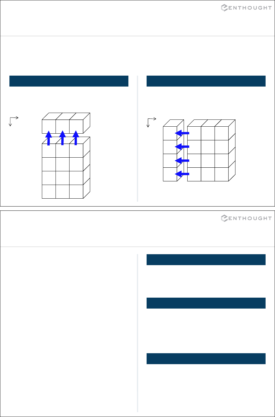
265
op.reduce()
>>> add.reduce(a)
array([60, 64, 68])
For multidimensional arrays, op.reduce(a,axis)applies op to the elements of
a along the specified axis. The resulting array has dimensionality one less than a.
The default value for axis is 0.
30 31 32
20 21 22
10 11 12
0 1 2
93
63
33
3
>>> add.reduce(a,1)
array([ 3, 33, 63, 93])
30 31 32
20 21 22
10 11 12
0 1 2
60 64 68
SUM COLUMNS BY DEFAULT SUMMING UP EACH ROW
1
0
1
0
266
op.accumulate()
>>> a = array([1,1,0])
>>> logical_and.accumulate(a)
array([True, True, False])
>>> logical_or.accumulate(a)
array([True, True, True])
op.accumulate(a) creates a
new array containing the intermediate
results of the reduce operation at
each element in a.
For example:
0
0
1
0
1
0
][],...,[],[
n
N
nn
nanana
late(a)add.accumuy
ADD EXAMPLE
>>> a = array([1,2,3,4])
>>> add.accumulate(a)
array([ 1, 3, 6, 10])
STRING LIST EXAMPLE
>>> a = array(['ab','cd','ef'],
... dtype=object)
>>> add.accumulate(a)
array([ab,abcd,abcdef],
dtype=object)
LOGICAL OP EXAMPLES
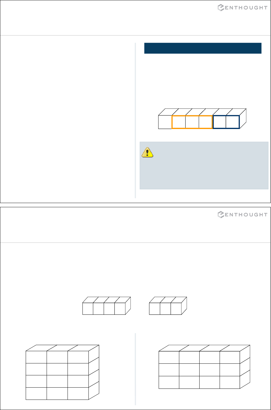
267
op.reduceat()
>>> a = array([0,10,20,30,
... 40,50])
>>> indices = array([1,4])
>>> add.reduceat(a,indices)
array([60, 90])
op.reduceat(a,indices)
applies op to ranges in the 1-D array a
defined by the values in indices.
The resulting array has the same length
as indices.
For multidimensional arrays,
reduceat() is always applied along the
last
axis (sum of rows for 2-D arrays).
This is different from the default for
reduce() and accumulate().
1 4
010 20 30 40 50
EXAMPLE
][
][
][y[i]
1iindices
iindicesn
na
For example:
y = add.reduceat(a, indices)
268
op.outer()
op.outer(a,b) forms all possible combinations of elements between
a and b using op. The shape of the resulting array results from
concatenating the shapes of a and b. (Order matters.)
>>> add.outer(a,b)
a[3]+b[0] a[3]+b[1] a[3]+b[2]
a[2]+b[0] a[2]+b[1] a[2]+b[2]
a[1]+b[0] a[1]+b[1] a[1]+b[2]
a[0]+b[0] a[0]+b[1] a[0]+b[2]
a b
b[0] b[1] b[2]a[0] a[1] a[2] a[3]
b[2]+a[0]
b[1]+a[0]
b[0]+a[0]
b[2]+a[1]
b[1]+a[1]
b[0]+a[1]
b[2]+a[2] b[2]+a[3]
b[1]+a[2] b[1]+a[3]
b[0]+a[2] b[0]+a[3]
>>> add.outer(b,a)
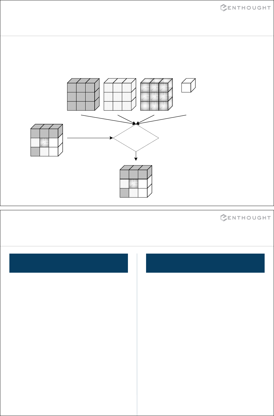
269
Array Functions – choose()
c0 c1 c2 c3
choice_array
0 1 3
1 3
0 0 0
6 7 8
3 4 5
0 1 2
5 5 5
5 5 5
5 5 5
2 2 2
2 2 2
2 2 2 9
2
6 5 9
5 9
0 1 2
2
choose()
y
>>> y = choose(choice_array,(c0,c1,c2,c3))
270
Example - choose()
>>> a < 10
array([[True, True, True],
[False, False, False],
[False, False, False],
dtype=bool)
>>> choose(a<10,(a,10))
array([[10, 10, 10],
[10, 11, 12],
[20, 21, 22]])
>>> lt = a < 10
>>> gt = a > 15
>>> choice = lt + 2 * gt
>>> choice
array([[1, 1, 1],
[0, 0, 0],
[2, 2, 2]])
>>> choose(choice,(a,10,15))
array([[10, 10, 10],
[10, 11, 12],
[15, 15, 15]])
>>> a
array([[ 0, 1, 2],
[10, 11, 12],
[20, 21, 22]])
CLIP LOWER AND UPPER
VALUES
CLIP LOWER VALUES TO 10
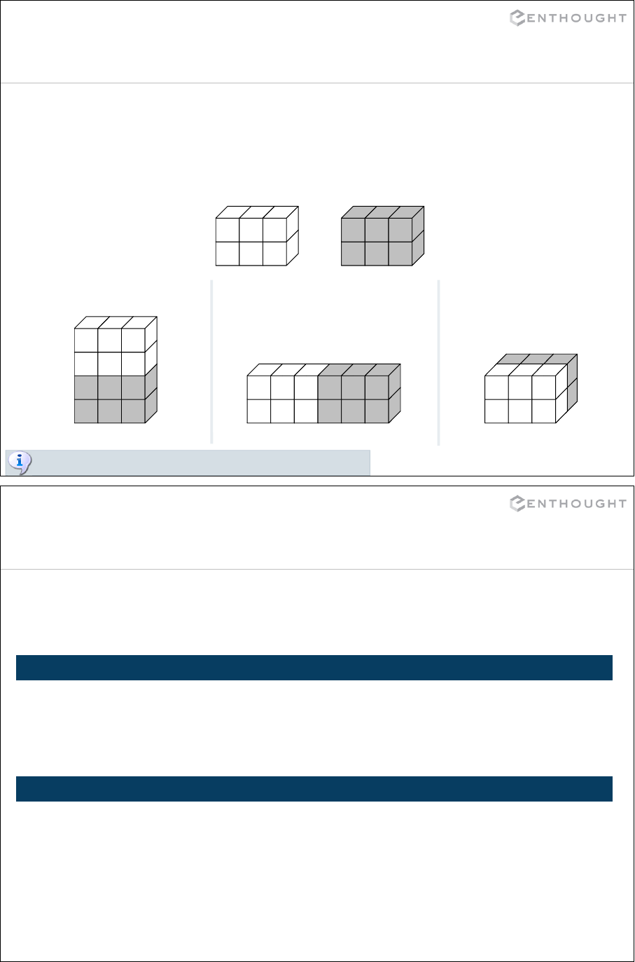
271
Array Functions – concatenate()
concatenate((a0,a1,…,aN),axis=0)
The input arrays (a0,a1,…,aN) are concatenated along the given
axis. They must have the same shape along every axis
except
the
one given.
10 11 12
0 1 2
60 61 62
50 51 52
60 61 62
50 51 52
10 11 12
0 1 2
60 61 62
50 51 52
10 11 12
0 1 2
10 11 12
0 1 2
60 61 62
50 51 52
x y
>>> concatenate((x,y)) >>> concatenate((x,y),1) >>> array((x,y))
See also vstack(), hstack() and dstack() respectively.
272
Array Broadcasting
NumPy arrays of different dimensionality can be combined in the same
expression. Arrays with smaller dimension are broadcasted to match the
larger arrays, without copying data. Broadcasting has two rules.
In [3]: a = ones((3, 5)) # a.shape == (3, 5)
In [4]: b = ones((5,)) # b.shape == (5,)
In [5]: b.reshape(1, 5) # result is a (1,5)-shaped array.
In [6]: b[newaxis, :] # equivalent, more concise.
RULE 1: PREPEND ONES TO SMALLER ARRAYS’ SHAPE
In [7]: c = a + b # c.shape == (3, 5)
is logically equivalent to...
In [8]: tmp_b = b.reshape(1, 5)
In [9]: tmp_b_repeat = tmp_b.repeat(3, axis=0)
In [10]: c = a + tmp_b_repeat
# But broadcasting makes no copies of “b”s data!
RULE 2: DIMENSIONS OF SIZE 1 ARE REPEATED WITHOUT COPYING
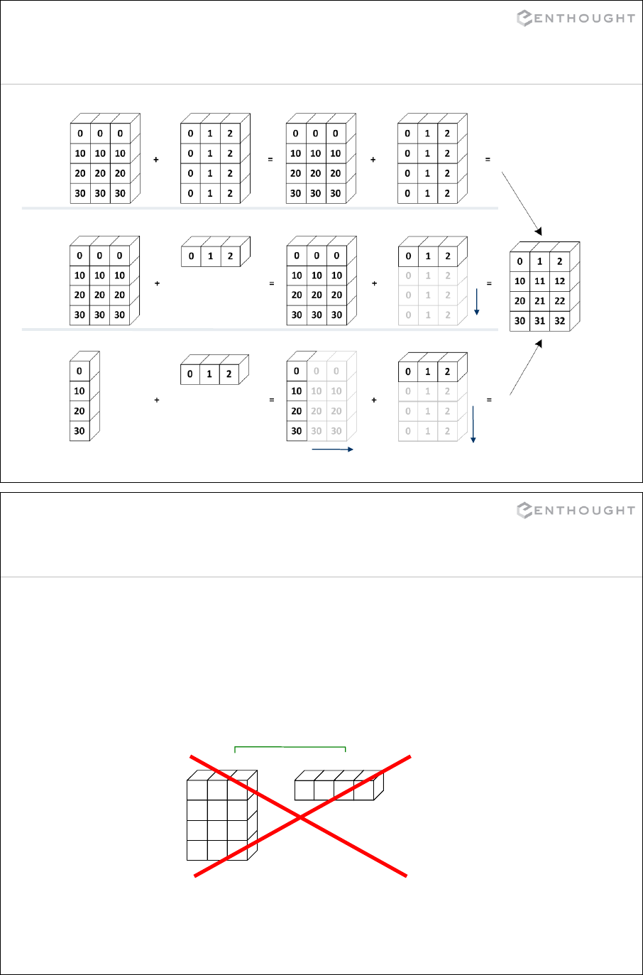
273
Array Broadcasting
stretch stretch
stretch
4x1 3
4x3 3
4x3 4x3
274
Broadcasting Rules
+
30 30 30
20 20 20
10 10 10
0 0 0 0 1 2
=
3
The
trailing
axes of either arrays must be 1 or both must have the same
size for broadcasting to occur. Otherwise, a
"ValueError: shape mismatch: objects cannot be
broadcast to a single shape" exception is thrown.
4x3 4
mismatch
!

275
Broadcasting in Action
>>> a = array((0,10,20,30))
>>> b = array((0,1,2))
>>> y = a[:, newaxis] + b
+
30
20
10
00 1 2
=
30 31 32
20 21 22
10 11 12
0 1 2
276
Application: distance from center
In [1]: a = linspace(0, 1, 15) - 0.5
In [2]: b = a[:, newaxis] # b.shape == (15, 1)
In [3]: dist2 = a**2 + b**2 # broadcasting sum.
In [4]: dist = sqrt(dist2)
In [5]: imshow(dist); colorbar()

277
Broadcasting’s usefulness
Broadcasting can often be used to replace needless data replication inside a
NumPy array expression.
np.meshgrid() – use newaxis appropriately in broadcasting expressions.
np.repeat() – broadcasting makes repeating an array along a dimension of
size 1 unnecessary.
In [3]: x, y = \
meshgrid([1,2],[3,4,5])
In [4]: z = x + y
MESHGRID: COPIES DATA
In [5]: x = array([1,2])
In [6]: y = array([3,4,5])
In [7]: z = \
x[newaxis,:] + y[:,newaxis]
BROADCASTING: NO COPIES
278
Vector Quantization Example
Feature 1
Feature 2
Target 1
Target 2
0
1
2
3
4
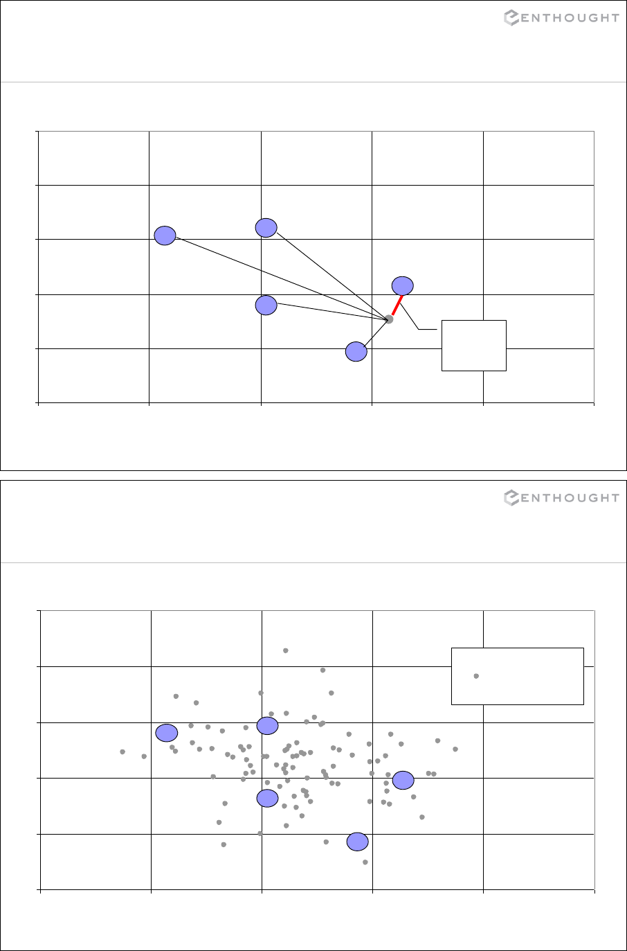
279
Vector Quantization Example
Feature 1
Feature 2
0
1
2
3
4
Minimum
Distance
280
Vector Quantization Example
Feature 1
Feature 2
Observations
0
1
2
3
4
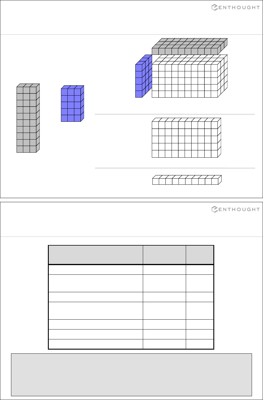
281
Vector Quantization Example
diff = obs[newaxis,:,:] – book[:,newaxis,:]
c1
c2
c3
c4
c0
Code Book
( book )
x y z
x
Observations
( obs )
y z
10x3
5x3
o1
o2
o3
o4
o0
o6
o7
o8
o9
o5
o1o2 o3o0 o5o6o4 o7o8 o9
distance = sqrt(sum(diff**2,axis=-1))
code_index = argmin(distance,axis=0))
5x10x3 1x10x3 5x1x3
282
VQ Speed Comparisons
Method Run Time
(sec) Speed
Up
Matlab 5.3 1.611 -
Python VQ1, double
2.245 0.71
Python VQ1, float 1.138 1.42
Python VQ2, double
1.637 0.98
Python VQ2, float 0.954 1.69
C, double 0.066 24.40
C, float 0.064 24.40
•4000 observations with 16 features categorized into 40 codes
on Pentium III 500 MHz.
•VQ1 uses the technique described on the previous slide verbatim.
•VQ2 applies broadcasting on an observation by observation basis.
This turned out to be much more efficient because it is less memory intensive.
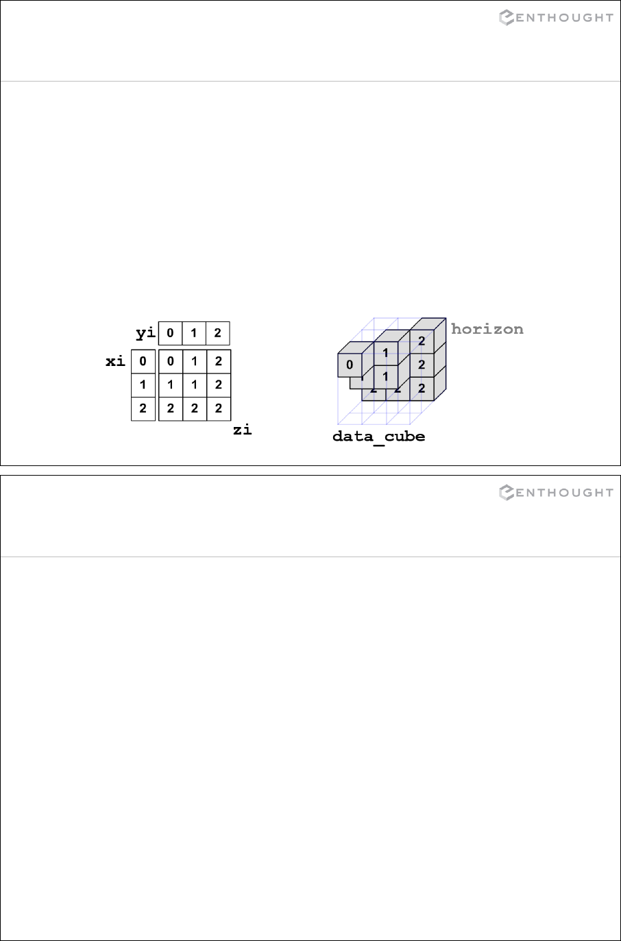
283
Broadcasting Indices
Broadcasting can also be used to slice elements from different
“depths” in a 3-D (or any other shape) array. This is a very powerful
feature of indexing.
>>> xi,yi = ogrid[:3,:3]
>>> zi = array([[0, 1, 2],
[1, 1, 2],
[2, 2, 2]])
>>> horizon = data_cube[xi,yi,zi]
Indices Selected Data
284
“Structured” Arrays
# "Data structure" (dtype) that describes the fields and
# type of the items in each array element.
>>> particle_dtype = dtype([('mass','float32'), ('velocity', 'float32')])
# This must be a list of tuples.
>>> particles = array([(1,1), (1,2), (2,1), (1,3)],
dtype=particle_dtype)
>>> print particles
[(1.0, 1.0) (1.0, 2.0) (2.0, 1.0) (1.0, 3.0)]
# Retrieve the mass for all particles through indexing.
>>> print particles['mass']
[ 1. 1. 2. 1.]
# Retrieve particle 0 through indexing.
>>> particles[0]
(1.0, 1.0)
# Sort particles in place, with velocity as the primary field and
# mass as the secondary field.
>>> particles.sort(order=('velocity','mass'))
>>> print particles
[(1.0, 1.0) (2.0, 1.0) (1.0, 2.0) (1.0, 3.0)]
# See demo/multitype_array/particle.py.
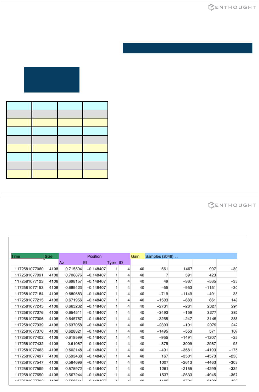
285
“Structured” Arrays
Brad Jane John Fred
33 25 47 54
135.0 105.0 225.0 140.0
Henry George Brian Amy
29 61 32 27
154.0 202.0 137.0 187.0
Ron Susan Jennifer Jill
19 33 18 54
188.0 135.0 88.0 145.0
name char[10]
age int
weight double
Elements of an array can be
any fixed-size data structure! EXAMPLE
>>> from numpy import dtype, empty
# structured data format
>>> fmt = dtype([('name', 'S10'),
('age', int),
('weight', float)
])
>>> a = empty((3,4), dtype=fmt)
>>> a.itemsize
22
>>> a['name'] = [['Brad', … ,'Jill']]
>>> a['age'] = [[33, … , 54]]
>>> a['weight'] = [[135, … , 145]]
>>> print a
[[('Brad', 33, 135.0)
…
('Jill', 54, 145.0)]]
286
Nested Datatype
nested.dat

287
Nested Datatype (cont’d)
>>> dt = dtype([('time', uint64),
... ('size', uint32),
... ('position', [('az', float32),
... ('el', float32),
... ('region_type', uint8),
... ('region_ID', uint16)]),
... ('gain', uint8),
... ('samples', int16, 2048)])
>>> data = loadtxt('nested.dat', dtype=dt, skiprows = 2)
>>> data['position']['az']
array([ 0.71559399, 0.70687598, 0.69815701, 0.68942302,
0.68068302, ...], dtype=float32)
The data file can be extracted with the following code:
288
Memory Mapped Arrays
•Methods for Creating:
–memmap: subclass of ndarray that manages the
memory mapping details.
–frombuffer: Create an array from a memory mapped
buffer object.
–ndarray constructor: Use the buffer keyword to
pass in a memory mapped buffer.
•Limitations:
–Files must be < 2GB on Python 2.4 and before.
–Files must be < 2GB on 32-bit machines.
–Python 2.5 and higher on 64 bit machines is
theoretically "limited" to 17.2 billion GB (17 Exabytes).
289
Memory Mapped Example
# Create a "memory mapped" array where
# the array data is stored in a file on
# disk instead of in main memory.
>>> from numpy import memmap
>>> image = memmap('some_file.dat',
dtype=uint16,
mode='r+',
shape=(5,5),
offset=header_size)
# Standard array methods work.
>>> mean_value = image.mean()
# Standard math operations work.
# The resulting scaled_image *is*
# stored in main memory. It is a
# standard numpy array.
>>> scaled_image = image * .5
image:
2D NumPy array
shape: 5, 5
dtype: uint16
some_file.dat
<header> 110111…
<data> 0110000001
0010010111011000
1101001001000100
1111010101000010
0010111000101011
00011110101011…
290
memmap
The memmap subclass of array handles opening and closing files as
well as synchronizing memory with the underlying file system.
memmap(filename, dtype=uint8, mode='r+',
offset=0, shape=None, order=0)
filename Name of the underlying file. For all modes, except for 'w+', the file must already exist
and contain at least the number of bytes used by the array.
dtype The numpy data type used for the array. This can be a "structured" dtype as well as
the standard simple data types.
offset Byte offset within the file to the memory used as data within the array.
mode <see next slide>
shape Tuple specifying the dimensions and size of each dimension in the array. shape=(5,10)
would create a 2D array with 5 rows and 10 columns.
order 'C' for row major memory ordering (standard in the C programming language) and 'F'
for column major memory ordering (standard in Fortran).

291
memmap -- mode
The mode setting for memmap arrays is used to set the access flag
when opening the specified file using the standard mmap module.
memmap(filename, dtype=uint8, mode='r+',
offset=0, shape=None, order=0)
mode A string indicating how the underlying file should be opened.
'r' or 'readonly': Open an existing file as an array for reading.
'c' or 'copyonwrite': "Copy on write" arrays are "writable" as Python arrays, but
they never modify the underlying file.
'r+' or 'readwrite': Create a read/write array from an existing file. The file will
have "write through" behavior where changes to the array are written to the
underlying file. Use the flush() method to ensure the array is
synchronized with the file.
'w+' or 'write': Create the file or overwrite if it exists. The array is filled
with zeros and has "write through" behavior similar to 'r+'.
292
memmap -- write through behavior
# Create a memory mapped "write through" file, overwriting it if it exists.
In [66]: q=memmap('new_file.dat',mode='w+',shape=(2,5))
In [67]: q
memmap([[0, 0, 0, 0, 0],
[0, 0, 0, 0, 0]], dtype=uint8)
# Print out the contents of the underlying file. Note: It
# doesn't print because 0 isn't a printable ascii character.
In [68]: !cat new_file.dat
# Now write the ascii value for 'A' (65) into our array.
In [69]: q[:] = ord('A')
In [70]: q
memmap([[65, 65, 65, 65, 65],
[65, 65, 65, 65, 65]], dtype=uint8)
# Ensure the OS has written the data to the file, and examine
# the underlying file. It is full of 'A's as we hope.
In [71]: q.flush()
In [72]: !cat new_file.dat
AAAAAAAAAA

293
memmap -- copy on write behavior
# Create a copy-on-write memory map where the underlying file is never
# modified. The file must already exist.
# This is a memory efficient way of working with data on disk as arrays but
# ensuring you never modify it.
In [73]: q=memmap('new_file.dat',mode='c',shape=(2,5))
In [74]: q
memmap([[65, 65, 65, 65, 65],
[65, 65, 65, 65, 65]], dtype=uint8)
# Set values in array to something new.
In [75]: q[1] = ord('B')
In [76]: q
memmap([[65, 65, 65, 65, 65],
[66, 66, 66, 66, 66]], dtype=uint8)
# Even after calling flush(), the underlying file is not updated.
In [77]: q.flush()
In [78]: !cat new_file.dat
AAAAAAAAAA
294
Using Offsets
# Create a memory mapped array with 10 elements.
In [1]: q=memmap('new_file.dat',mode='w+', dtype=uint8, shape=(10,))
In [2]: q[:] = arange(0,100,10)
memmap([ 0, 10, 20, 30, 40, 50, 60, 70, 80, 90], dtype=uint8)
# Now, create a new memory mapped array (read only) with an offset into
# the previously created file.
In [3]: q=memmap('new_file.dat',mode='r', dtype=uint8, shape=6, offset=4)
In [4]: q
memmap([40, 50, 60, 70, 80, 90], dtype=uint8)
# The number of bytes required by the array must be equal or less than
# the number of bytes available in the file.
In [3]: q=memmap('new_file.dat',mode='r', dtype=uint8, shape=7, offset=4)
ValueError: mmap length is greater than file size
0 10 20 30 40 50 60 70 80 90
new_file.dat
0 10 20 30 40 50 60 70 80 90
new_file.dat
295
64 bit floating point data…
Working with file headers
# Create a dtype to represent the header.
header_dtype = dtype([('rows', int32), ('cols', int32)])
# Create a memory mapped array using this dtype. Note the shape is empty.
header = memmap(file_name, mode='r', dtype=header_dtype, shape=())
# Read the row and column sizes from using this structured array.
rows = header['rows']
cols = header['cols']
# Create a memory map to the data segment, using rows, cols for shape
# information and the header size to determine the correct offset.
data = memmap(file_name, mode='r+', dtype=float64,
shape=(rows, cols), offset=header_dtype.itemsize)
rows (int32)
data
header
File Format: cols (int32)
296
64 bit floating point data…
memory maps with ndarray
# mmap is a standard Python module for working with memory maps.
import mmap
import numpy
# Create a dtype to represent the header.
header_dtype = numpy.dtype([('rows', int32), ('cols', int32)])
# Open a file for read/write access in binary mode.
file = open(file_name,'r+b')
# Create a read-only memory map from the opened file with the
# correct size to read the header of the file.
mm = mmap.mmap(file.fileno(), header_dtype.itemsize,
access=mmap.ACCESS_READ)
< continued >
rows (int32)
data
header
File Format: cols (int32)
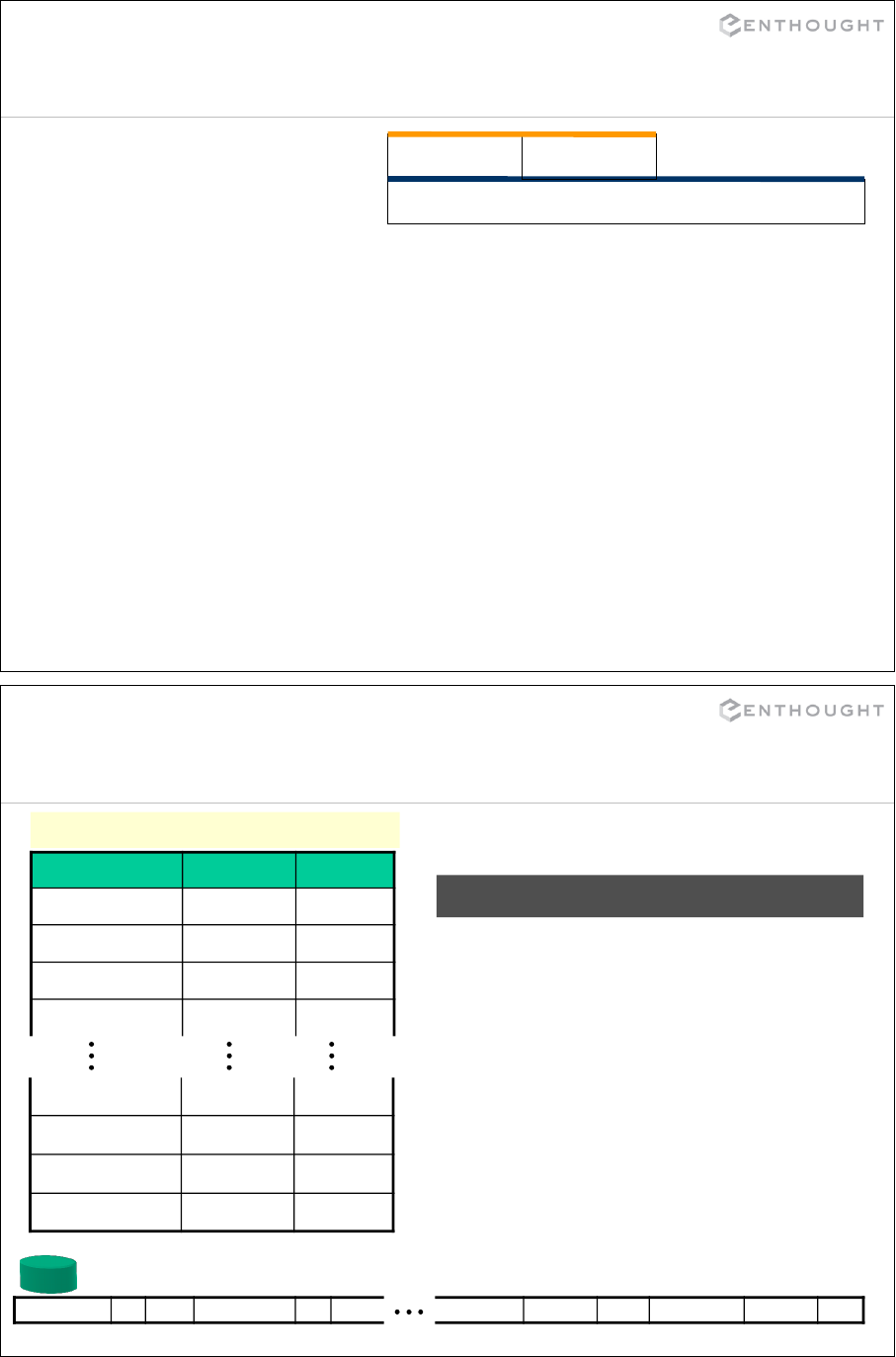
297
64 bit floating point data…
memory maps with ndarray
# Create a new array using the ndarray constructor.
# The first argument is the shape, and we pass in the data type and the
# memory buffer to use (mm) as keyword arguments.
header = numpy.ndarray((), dtype=header_dtype, buffer=mm)
rows = header['rows']
cols = header['cols']
# Create a writable memory map to use for the data array. The size of the
# memory map in bytes is the size of a float64 (8) * rows * columns.
mm = mmap.mmap(file.fileno(), 8*rows*cols, access=mmap.ACCESS_WRITE)
# Create our data array using this new memory map. Start the arrays
# data at the memory location directly after the header using offset.
data = numpy.ndarray((rows, cols), dtype=float64, buffer=mm,
offset=header_dtype.itemsize)
rows (int32)
data
header
File Format: cols (int32)
298
Structured Arrays
Example
Elements of array can be any
fixed-size data structure!
char[12] int64 float32
Name Time Value
MSFT_profit 10 6.20
GOOG_profit 12 -1.08
MSFT_profit 18 8.40
INTC_profit 25 -0.20
GOOG_profit 1000325 3.20
GOOG_profit 1000350 4.50
INTC_profit 1000385 -1.05
MSFT_profit 1000390 5.60
>>> import numpy as np
>>> fmt = np.dtype([('name', 'S12'),
('time', np.int64),
('value', np.float32)])
>>> vals = [('MSFT_profit', 10, 6.20),
('GOOG_profit', 12, -1.08),
('INTC_profit', 1000385, -1.05)
('MSFT_profit', 1000390, 5.60)]
>>> arr = np.array(vals, dtype=fmt)
# or
>>> arr = np.fromfile('db.dat', dtype=fmt)
# or
>>> arr = np.memmap('db.dat', dtype=fmt,
mode='c')
…
MSFT_profit 10 6.20 GOOG_profit 12 -1.08
Disk
INTC_profit 1000385 -1.05 MSFT_profit 1000390 5.60
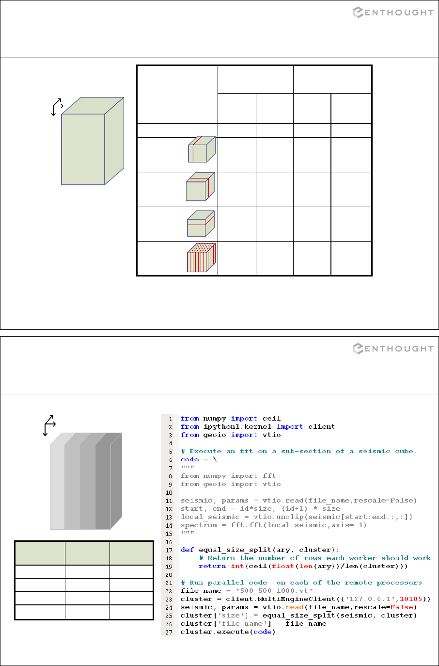
299
Memmap Timings (3D arrays)
500
500
1000
500 MB
file
(16 bit)
z
x
y
Operations
(500x500x1000)
Linux OS X
In
Memory Memory
Mapped In
Memory Memory
Mapped
read 2103 ms 11.0 ms 3505.00 27.00
x slice 1.8 ms 4.8 ms 1.80 8.30
y slice 2.8 ms 4.6 ms 4.40 7.40
z slice 9.2 ms 13.8 ms 10.40 18.70
downsample
4x4 0.02 ms 125 ms 0.02 198.70
Linux: Ubuntu 4.10, Dell Precision 690, Dual Quad Core Zeon X5355 2.6 GHz, 8 GB Memory
OS X: OS X 10.5, MacBook Pro Laptop, 2.6 GHz Core Duo, 4 GB Memory
All times in millesconds (ms).
300
Parallel FFT On Memory Mapped File
z
x
y
P 1
P 2
P 3
P 4
500 MB
Data File
Processors Time
(seconds) Speed Up
1 11.75 1.0
2 6.06 1.9
4 3.36 3.5
8 2.50 4.7

301
Controlling Output Format
set_printoptions(precision=None, threshold=None,
edgeitems=None, linewidth=None,
suppress=None)
precision The number of digits of precision to use for floating point output.
The default is 8.
threshold Array length where NumPy starts truncating the output and prints
only the beginning and end of the array. The default is 1000.
edgeitems Number of array elements to print at beginning and end of array
when threshold is exceeded. The default is 3.
linewidth Characters to print per line of output. The default is 75.
suppress Indicates whether NumPy suppresses printing small floating point
values in scientific notation. The default is False.
302
Controlling Output Formats
>>> a = arange(1e6)
>>> a
array([ 0.00000000e+00, 1.00000000e+00, 2.00000000e+00, ...,
9.99997000e+05, 9.99998000e+05, 9.99999000e+05])
>>> set_printoptions(precision=3)
>>> a
array([ 0.000e+00, 1.000e+00, 2.000e+00, ...,
1.000e+06, 1.000e+06, 1.000e+06])
PRECISION
>>> set_printoptions(precision=8)
>>> a = array((1, 2, 3, 1e-15))
>>> a
array([ 1.00000000e+00, 2.00000000e+00, 3.00000000e+00,
1.00000000e-15])
>>> set_printoptions(suppress=True)
>>> a
array([ 1., 2., 3., 0.])
SUPPRESSING SMALL NUMBERS

303
Controlling Error Handling
seterr(all=None, divide=None, over=None,
under=None, invalid=None)
all All error types to the specified value
divide Divide-by-zero errors
over Overflow errors
under Underflow errors
invalid Invalid floating point errors
Set the error handling flags in ufunc operations on a per thread basis.
Each of the keyword arguments can be set to ‘ignore’, ‘warn’, ‘print’, ‘log’,
‘raise’, or ‘call’.
304
Controlling Error Handling
>>> a = array((1,2,3))
>>> a/0.
Warning: divide by zero encountered in divide
array([ 1.#INF0000e+000, 1.#INF0000e+000, 1.#INF0000e+000])
# Ignore division-by-zero. Also, save old values so that
# we can restore them.
>>> old_err = seterr(divide='ignore')
>>> a/0.
array([ 1.#INF0000e+000, 1.#INF0000e+000, 1.#INF0000e+000])
# Restore original error handling mode.
>>> old_err
{'divide': 'print', 'invalid': 'print', 'over': 'print',
'under': 'ignore'}
>>> seterr(**old_err)
>>> a/0.
Warning: divide by zero encountered in divide
array([ 1.#INF0000e+000, 1.#INF0000e+000, 1.#INF0000e+000])
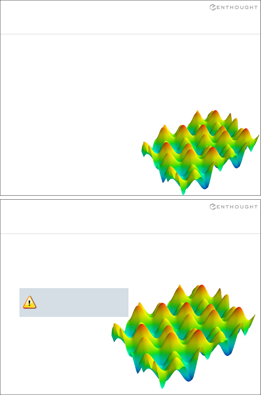
305
Interactive 3D Visualization
with
Mayavi-mlab
306
3D Visualization with Mayavi
C:\ ipython –-pylab
>>> from mayavi import mlab
matplotlib also has an mlab
namespace. Be sure you are using
the one from mayavi
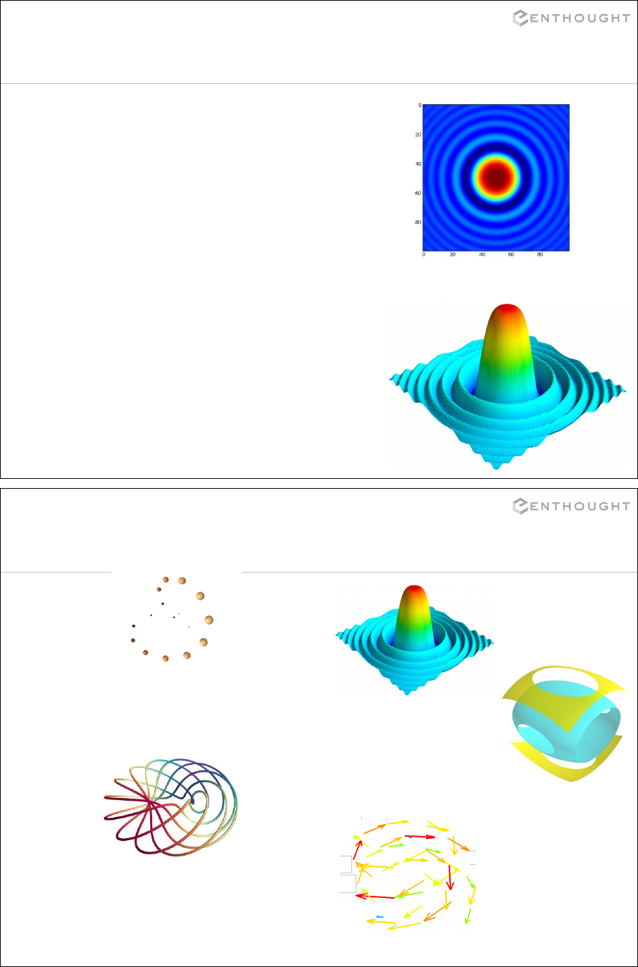
307
Interactive Example
# create arrays
>>> x, y = mgrid[-5:5:100j,-5:5:100j]
>>> r = x**2 + y**2
>>> z = sin(r)/r
# plot with mayavi
>>> from mayavi import mlab
>>> mlab.surf(x,y,5*z)
# plot with pylab
>>> imshow(z)
308
Some Plotting Commands
0D data
mlab.points3d(x, y, z)
1D data
mlab.plot3d(x, y, z)
3D data
mlab.contour3d(x, y, z)
Vector field
mlab.quiver(x, y, z, u, v, w)
2D data
mlab.surf(x, y, z)
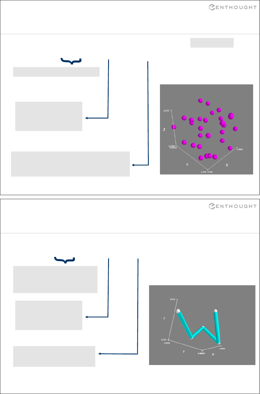
309
Points in 3D
mlab.points3d(x, y, z, color=(1.0,0.0,1.0), mode=‘sphere’, scale_factor=0.1)
x.shape == y.shape == z.shape
color = (R, G, B)
0.0 <= R, G, B <= 1.0
default is (1.0, 1.0, 1.0)
mode = ‘sphere’, ‘cone’, ‘cube’, ‘arrow’, ‘cylinder’, ‘point’,
‘2darrow’, ‘2dcircle’, ‘2dcross’, ‘2ddash’, ‘2ddiamond’,
‘2dhooked_arrow’, ‘2dsquare’, ‘2dthick_arrow’,
‘2dthick_cross’, ‘2dtriangle’, ‘2dvertex’
scaling applied
from numpy.random import rand
x,y,z = rand(30),rand(30),rand(30)
mlab.axes()
310
Lines in 3D
mlab.plot3d(x, y, z, color=(0.0,1.0,1.0), tube_radius=0.03)
1-d arrays giving end-points of
connected line-segments
len(x) == len(y) == len(z)
color = (R, G, B)
0.0 <= R, G, B <= 1.0
default is (1.0, 1.0, 1.0)
A float giving the radius of the
tubes representing the lines.
default is 0.025
from numpy.random import rand
x,y,z = rand(5), rand(5), rand(5)
mlab.points3d(x,y,z,scale_factor=0.06)
mlab.axes()
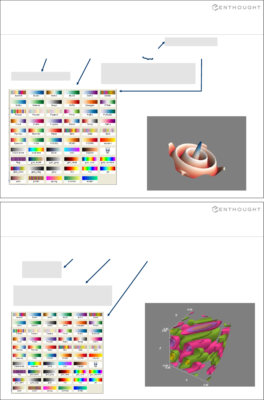
311
Surfaces in 3D
mlab.surf(z, colormap=‘RdBu’) or mlab.surf(x, y, z, colormap=‘RdBu’)
2d array of “heights”
1d (or 2d) arrays producing a (possibly
non-uniform) orthogonal grid (such as
returned from ogrid or mgrid)
2d array of “heights”
from numpy import ogrid, hypot
from scipy.special import j0
x,y = ogrid[-15:15:100j, -15:15:100j]
z = j0(hypot(x,y))
312
Volumes in 3D
mlab.contour3d(data, contours=6, colormap=‘Dark2’)
3d array of
volume data
from numpy import ogrid, tanh, cos
from scipy.special import j0
x,y,z = ogrid[-5:5:64j, -5:5:64j,
-5:5:64j]
data = cos(0.5*y)*j0(x+y*1.3)*sin(0.8*z)
mlab.axes(ranges=[-5,5]*3)
Integer number of contours or
List of specific contours
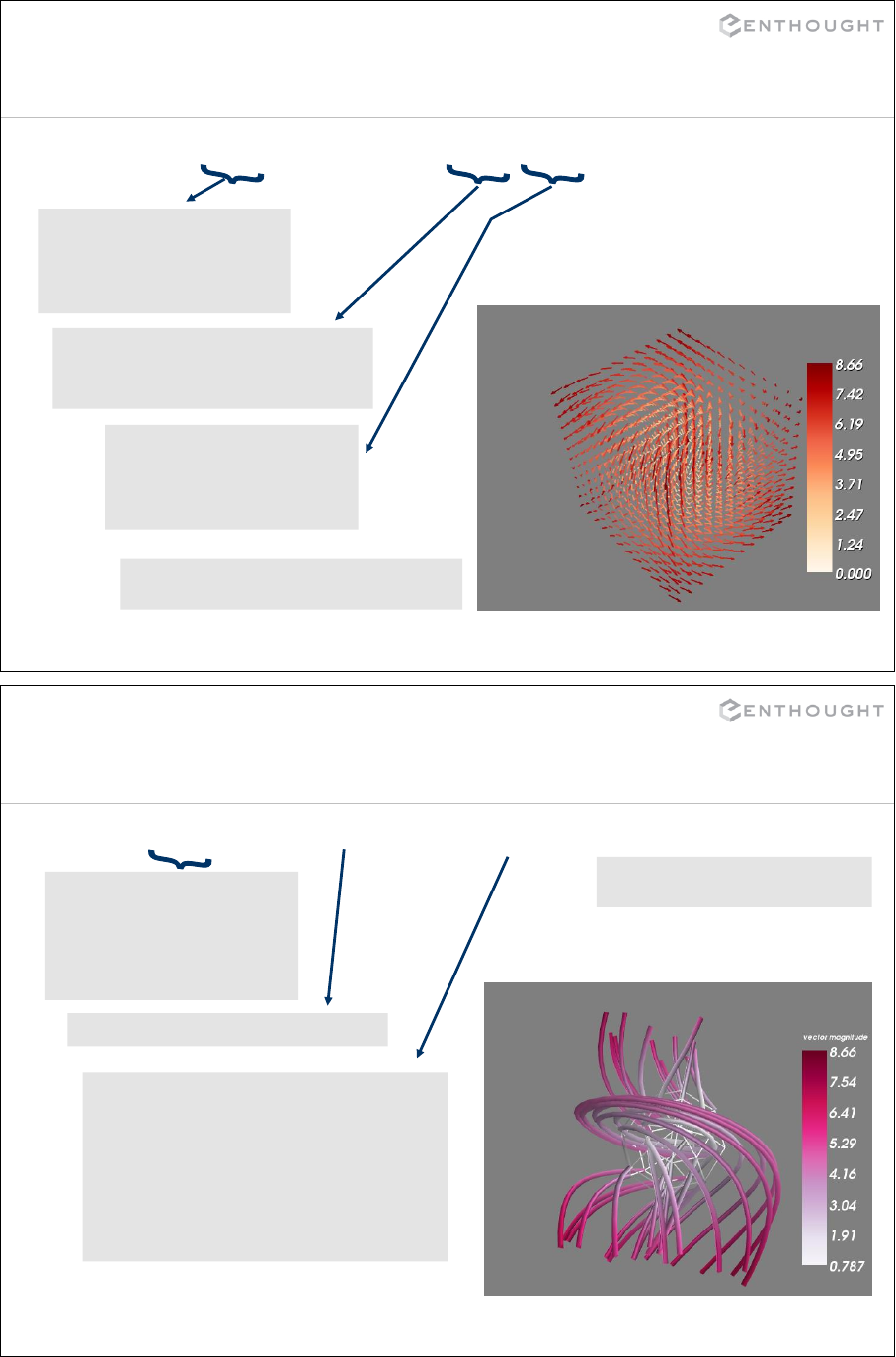
313
Vector Fields in 3D – quiver3d
mlab.quiver3d(u, v, w) or mlab.quiver3d(x, y, z, u, v, w)
3-d arrays each
representing a component
of a 3-d vector field. All
must be the same shape.
1, 2, or 3-d arrays of the same
shape as u, v, and w providing
real locations of the vectors.
from numpy import mgrid
x,y,z = mgrid[-5:5:12j, -5:5:12j, -5:5:12j]
u,v,w = -z, y, x
mlab.quiver3d(u,v,w, colormap=‘OrRd’)
any colormap argument will color glyphs
according to magnitude of vector.
1, 2, or 3-d arrays of the
same shape as x, y, and z
representing components
of the vectors.
314
Vector Fields in 3D – flow
mlab.flow(u, v, w, linetype=‘tube’, seedtype=‘sphere’, colormap=‘PuRd’)
3-d arrays representing
vector field. Can also be
called with x,y,z,u,v,w
where x, y, and z are all
3-d arrays.
linetype= ‘line’, ‘ribbon’, or ‘tube’
from numpy import mgrid
x,y,z = mgrid[-5:5:12j, -5:5:12j, -5:5:12j]
u,v,w = -z, y, x
any colormap argument will color
according to magnitude of vector.
seedtype = ‘sphere’, ‘plane’, ‘line’, or
‘point’
streamlines are calculated from
seedpoints spaced throughout the
specified seed widget. The seed
widget is shown and can be interacted
with to compute new streamlines.
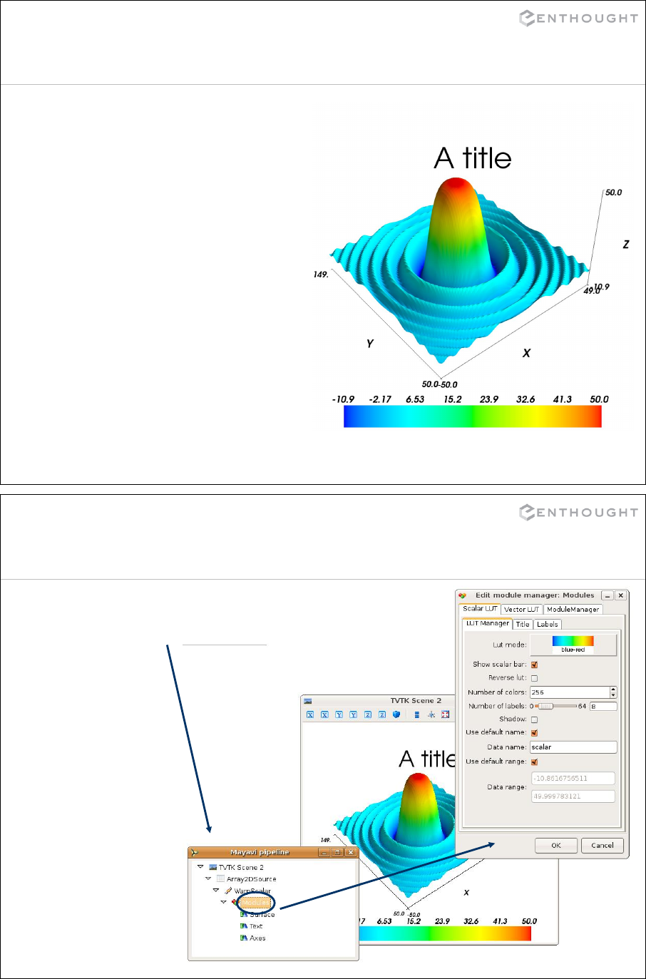
315
Figure Decorations
>>> mlab.title('A title')
>>> mlab.axes()
>>> mlab.colorbar()
>>> zlabel('Depth')
>>> mlab.clf()
>>> mlab.figure()
>>> mlab.gcf()
316
Graphical User Interface
mlab.show_pipeline()
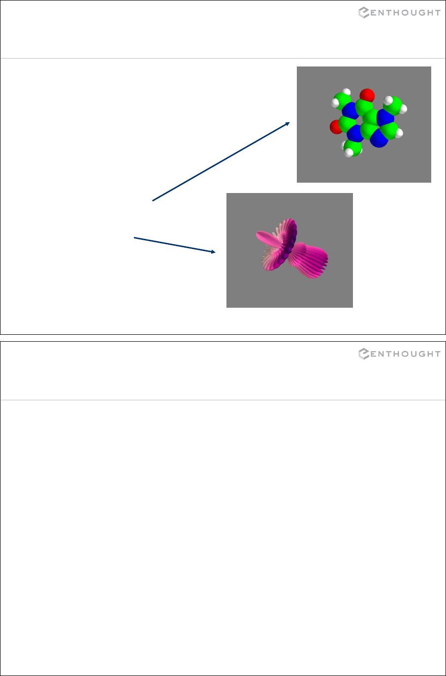
317
Examples and Demos
>>> mlab.test_<TAB>
mlab.test_points3d()
mlab.test_plot3d()
mlab.test_surf()
mlab.test_contour3d()
mlab.test_quiver3d()
mlab.test_molecule()
mlab.test_flow()
mlab.test_mesh()
Use ?? in IPython to look at the
source code of these examples.
318
Scientific Analysis
with
SciPy
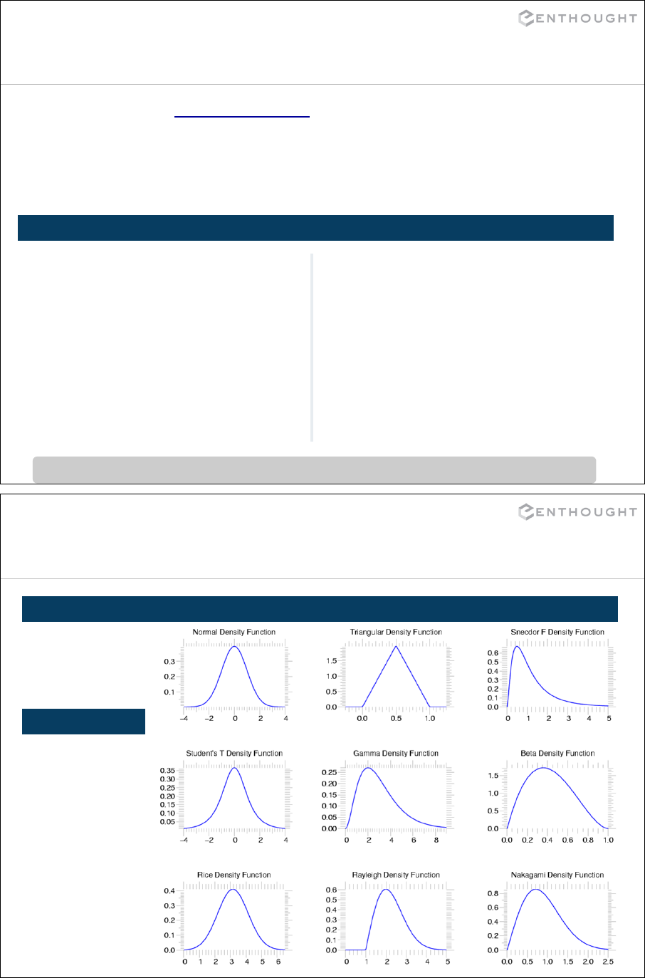
319
Overview
CURRENT PACKAGES
•Available at www.scipy.org
•Open source BSD style license
•38 contributors to the project in 2011
•Special Functions (scipy.special)
•Signal Processing (scipy.signal)
•Image Processing (scipy.ndimage)
•Fourier Transforms (scipy.fftpack)
•Optimization (scipy.optimize)
•Numerical Integration (scipy.integrate)
•Linear Algebra (scipy.linalg)
•Input/Output (scipy.io)
•Statistics (scipy.stats)
•Fast Execution (scipy.weave)
•Clustering Algorithms (scipy.cluster)
•Sparse Matrices (scipy.sparse)
•Interpolation (scipy.interpolate)
•...and more.
Note: “import scipy” does NOT import all these packages. Must be imported individually
320
Statistics
scipy.stats — CONTINUOUS DISTRIBUTIONS
over 80
continuous
distributions!
pdf
cdf
rvs
ppf
stats
fit
sf
isf
METHODS
entropy
nnlf
moment
freeze
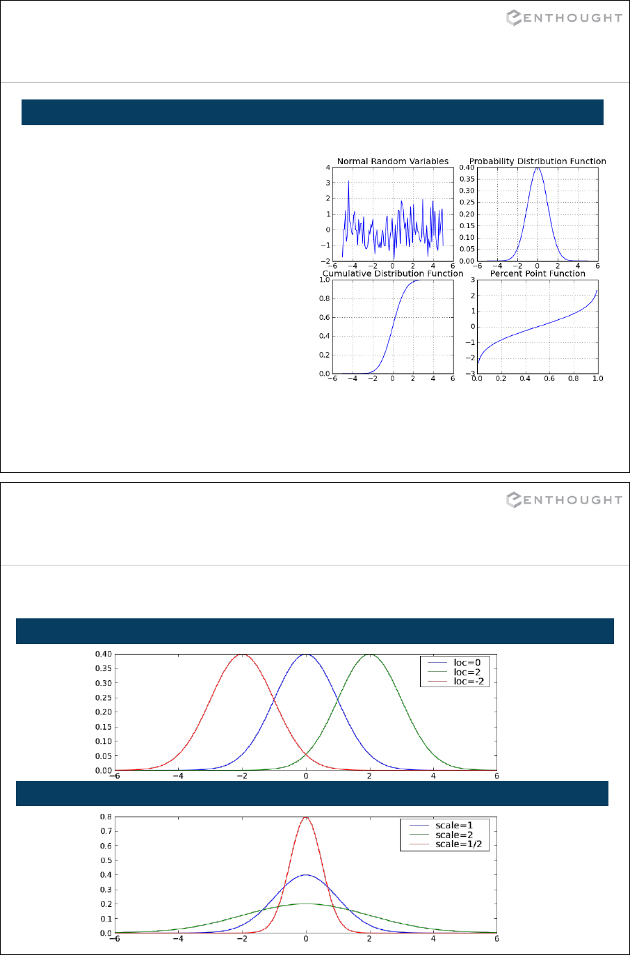
321
Using stats objects
>>> from scipy.stats import norm
# Sample normal dist. 100 times.
>>> samp = norm.rvs(size=100)
>>> x = linspace(-5, 5, 100)
# Calculate probability dist.
>>> pdf = norm.pdf(x)
# Calculate cumulative dist.
>>> cdf = norm.cdf(x)
>>> x = linspace(0, 1, 100)
# Calculate Percent Point Function
>>> ppf = norm.ppf(x)
DISTRIBUTIONS
322
Distribution objects
Every distribution can be modified by loc and scale keywords
(many distributions also have required shape arguments to select from a family)
LOCATION (loc) --- shift left (<0) or right (>0) the distribution
SCALE (scale) --- stretch (>1) or compress (<1) the distribution
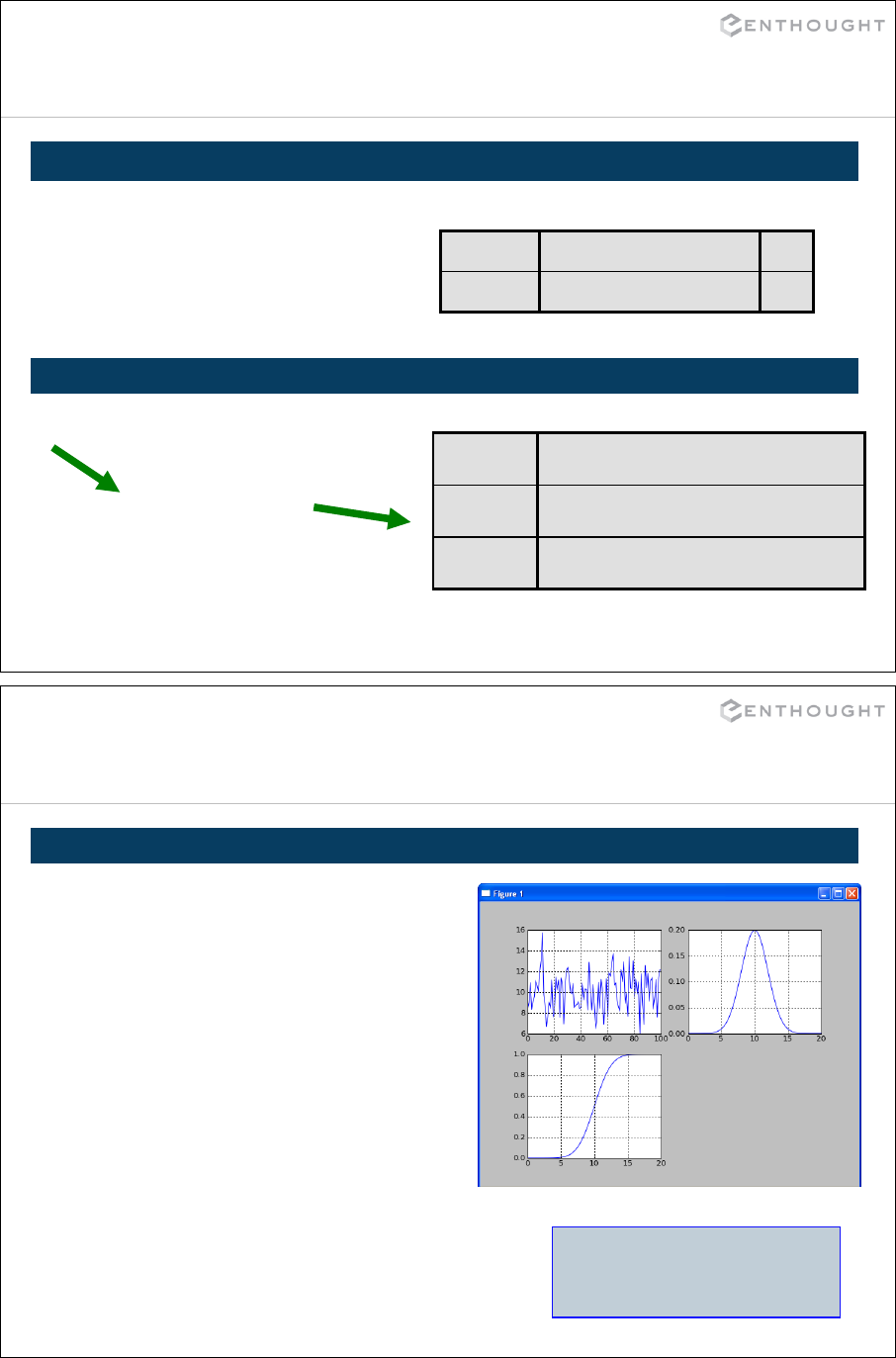
323
Example distributions
location offset from zero (rarely used)
scale e
shape
NORM (norm) – N(,)
Only location and scale
arguments:
LOG NORMAL (lognorm)
S is lognormal
location mean
scale standard deviation
log(S) is N(, )
one shape parameter!
324
Setting location and Scale
>>> from scipy.stats import norm
# Normal dist with mean=10 and std=2
>>> dist = norm(loc=10, scale=2)
>>> x = linspace(-5, 15, 100)
# Calculate probability dist.
>>> pdf = dist.pdf(x)
# Calculate cumulative dist.
>>> cdf = dist.cdf(x)
# Get 100 random samples from dist.
>>> samp = dist.rvs(size=100)
# Estimate parameters from data
>>> mu, sigma = norm.fit(samp)
>>> print “%4.2f, %4.2f” % (mu, sigma)
10.07, 1.95
NORMAL DISTRIBUTION
.fit returns best
shape + (loc, scale)
that explains the data
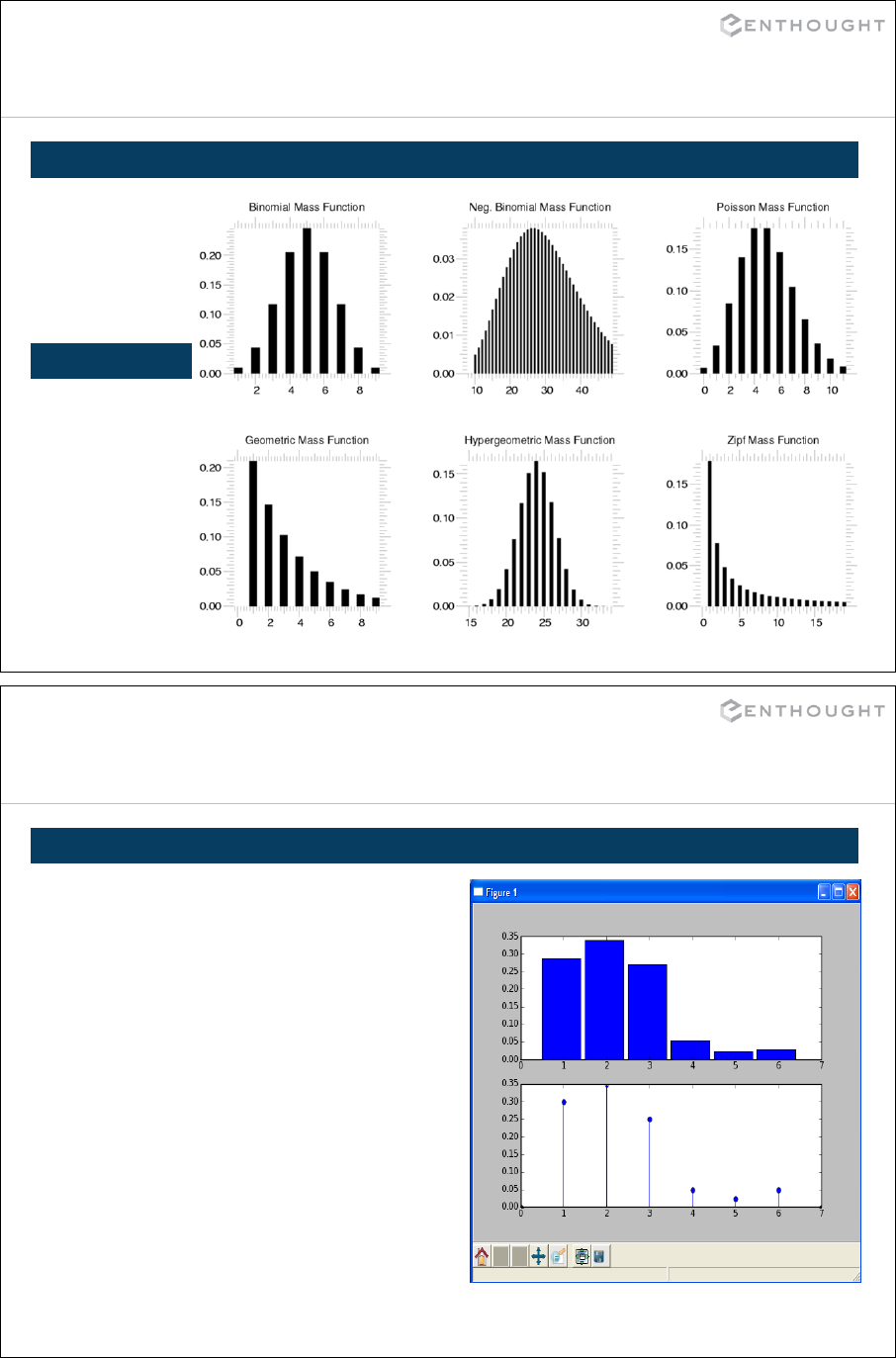
325
Statistics
scipy.stats — Discrete Distributions
10 standard
discrete
distributions
(plus any
finite RV)
pmf
cdf
rvs
ppf
stats
sf
isf
METHODS
moment
entropy
freeze
326
Using stats objects
# Create loaded dice.
>>> from scipy.stats import rv_discrete
>>> xk = [1, 2, 3, 4, 5, 6]
>>> pk = [0.3, 0.35, 0.25, 0.05,
0.025, 0.025]
>>> new = rv_discrete(name='loaded',
values=(xk,pk))
# Calculate histogram
>>> samples = new.rvs(size=1000)
>>> bins = linspace(0.5, 6.5, 7)
>>> subplot(211)
>>> hist(samples, bins=bins, normed=True)
# Calculate pmf
>>> x = range(0, 8)
>>> subplot(212)
>>> stem(x,new.pmf(x))
CREATING NEW DISCRETE DISTRIBUTIONS
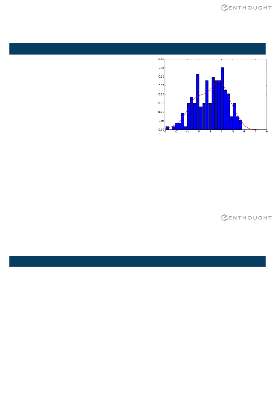
327
Statistics
# Sample two normal distributions
# and create a bimodal distribution
>>> rv1 = stats.norm()
>>> rv2 = stats.norm(2.0, 0.8)
>>> samples = hstack([rv1.rvs(size=100),
rv2.rvs(size=100)])
# Use a Gaussian kernel density to
# estimate the PDF for the samples.
>>> from scipy.stats.kde import gaussian_kde
>>> approximate_pdf = gaussian_kde(samples)
>>> x = linspace(-3, 6, 200)
# Compare the histogram of the samples to
# the PDF approximation.
>>> hist(samples, bins=25, normed=True)
>>> plot(x, approximate_pdf(x), 'r')
CONTINUOUS DISTRIBUTION ESTIMATION USING GAUSSIAN KERNELS
328
Linear Algebra
scipy.linalg — FAST LINEAR ALGEBRA
•Uses optimized BLAS and MKL if available — very fast
•Low-level access to BLAS and LAPACK routines in
modules linalg.blas, and linalg.lapack (FORTRAN order)
•High level matrix routines
•Linear Algebra Basics: inv, pinv, solve, det, norm,
lstsq, ...
•Decompositions: eig, lu, svd, orth, cholesky, qr,
schur, ...
•Matrix Functions: expm, logm, sqrtm, cosm, coshm, funm
(general matrix functions)

329
Solving A*X = B
SOLVE Ax=b LEAST SQUARES Ax=b
>>> from scipy import linalg
>>> a = array([[1.0, 3.0, 2.0],
... [4.0, 0.0, 1.0],
... [2.0, 2.0, 2.0]])
>>> b = array([2.0, 1.0, 0.0])
>>> x = linalg.solve(a, b)
>>> x
array([ 1.5, 3.5, -5. ])
# Check:
>>> dot(a, x)
array([ 2., 1., 0.])
# Over-specified problem:
>>> a = array([[1.0, 4.0],
... [3.0, 0.0],
... [2.0, 1.0]])
>>> b = array([2.0, 1.0, 0.0])
>>> x, res, rnk, svals = \
... linalg.lstsq(a, b)
# Least squares solution:
>>> x
array([ 0.1832, 0.4059])
# Sum of squared residuals:
>>> res
0.83663366336633671
# Effective rank of `a`:
>>> rnk
2
# Singular values of `a`:
>>> svals
array([ 4.6567, 3.0521])
330
To solve many equations AX=B for different
matrices B, factor A =L*U , L is lower
triangular (L) and U is upper-triangular
>>> from scipy import linalg
>>> a = array([[1,3,5],
... [2,5,1],
... [2,3,6]])
# time consuming factorization
>>> lu, piv = linalg.lu_factor(a)
# fast solve for 1 or more
# right hand sides.
>>> b = array([10,8,3])
>>> linalg.lu_solve((lu, piv), b)
array([-7.82608696, 4.56521739,
0.82608696])
# check
>>> dot(a, _)
array([ 10., 8., 3.])
LU FACTORIZATION
>>> a = array([[12, -51, 4],
... [ 6, 167, -68],
... [-4, 24, -41]])
>>> q, r = linalg.qr(a)
>>> q
array([[-0.8571, 0.3943, 0.3314],
[-0.4286, -0.9029, -0.0343],
[ 0.2857, -0.1714,
0.9429]])
>>> r
array([[ -14., -21., 14.],
[ 0., -175., 70.],
[ -0., 0., -35.]])
QR FACTORIZATION
To solve Ax=b, factor A = QR, where Q is
orthogonal and R is upper triangular.
See the qr docstring for more advanced
options (e.g. pivoting for rank-revealing QR
decomposition).
Factorizations

331
Eigenvalues, eigenvectors
SCHUR DECOMPOSITION
>>> t, z = linalg.schur(a)
>>> t
array(
[[ 156.137, 64.737, 85.651],
[ 0. , 16.06 , 15.814],
[ 0. , 0. , -34.197]])
>>> z
array([[ 0.328, -0.94 , 0.098],
[-0.937, -0.337, -0.093],
[-0.121, 0.061, 0.991]])
# Diagonals in t are eigenvalues:
>>> linalg.eigvals(a)
array([ 156.137+0.j, 16.060+0.j,
-34.197+0.j])
Factor A = ZTZ-1, where Z is unitary and T is
upper triangular.
EIGENVALUES AND VECTORS
>>> a = array([[1,3,5],
... [2,5,1],
... [2,3,6]])
# compute eigenvalues/vectors
>>> vals, vecs = linalg.eig(a)
# print eigenvalues
>>> vals
array([ 9.39895873+0.j,
-0.73379338+0.j,
3.33483465+0.j])
# eigenvectors are in columns
# print first eigenvector
>>> vecs[:,0]
array([-0.57028326,
-0.41979215,
-0.70608183])
# norm of vector should be 1.0
>>> linalg.norm(vecs[:,0])
1.0
332
Linear Algebra
>>> a = array([[2, 1],
... [2, 0]])
>>> u, s, vt = linalg.svd(a)
>>> u
array([[-0.75 , -0.662],
[-0.662, 0.75 ]])
# s holds the singular values.
>>> s
array([ 2.921, 0.685])
>>> vt
array([[-0.966, -0.257],
[ 0.257, -0.966]])
# Use to inverse A
>>> inv_a = dot(vt.T,
dot(diag(1/s), u.T))
>>> dot(a, inv_a)
array([[ 1.0, -4.44089210e-16],
[ -2.22044605e-16, 1.0]])
SINGULAR VALUE DECOMPOSITION
# Nonsquare example:
underspecified
# set of equations
>>> a = array([[2, 1, -4],
[2, 3, 1]])
>>> u, s, vt = linalg.svd(a)
>>> u
array([[-0.938, -0.347],
[-0.347, 0.938]])
>>> s
array([ 4.702, 3.59 ])
>>> vt
array([[-0.546, -0.421, 0.724],
[ 0.329, 0.687, 0.648],
[ 0.77 , -0.592, 0.237]])
Factor A = U S V*, where U and V are unitary, and S is diagonal. This generalizes diagonalization.

# Non-square mat: Pseudo-inverse
# with least-square method
>>> b = array([[2, 1, -4],
[2, 3, 1]])
>>> linalg.pinv(b)
array([[ 0.07719298,
0.12631579],
[ 0.01754386,
0.21052632],
[-0.20701754,
0.11578947]])
>>> linalg.det(a)
-2.0
#If LU decomposition available:
>>> lu, _ = linalg.lu_factor(a)
>>> np.prod(lu.diagonal())
-2.0
Inverse, and determinants
333
# Square matrix
>>> from scipy import linalg
>>> a = array([[2, 1],
... [2, 0]])
>>> a_inv = linalg.inv(a)
>>> a_inv
array([[ 0. , 0.5],
[ 1. , -1. ]])
# Check
>>> dot(a, a_inv)
array([[ 1., 0.],
[ 0., 1.]])
# Alternatively (slower)
>>> linalg.solve(a, indentity(2))
array([[ 0. , 0.5],
[ 1. , -1. ]])
MATRIX INVERSION
MATRIX DETERMINANT
334
Matrix Objects
SOLVE
>>> from numpy import mat
>>> a = mat('[1,3,5;2,5,1;2,3,6]')
>>> a
matrix([[1, 3, 5],
[2, 5, 1],
[2, 3, 6]])
STRING CONSTRUCTION
INVERTED ATTRIBUTE
TRANSPOSE ATTRIBUTE
DIAGONAL
>>> a.T
matrix([[1, 2, 2],
[3, 5, 3],
[5, 1, 6]])
>>> a.I
matrix([[-1.1739, 0.1304, 0.956],
[ 0.4347, 0.1739, -0.391],
[ 0.1739, -0.130, 0.0434]
])
>>> a.diagonal()
matrix([[1, 5, 6]])
>>> a.diagonal(-1)
matrix([[2, 3]])
>>> b = mat('10;8;3')
>>> a.I*b
matrix([[-7.82608696],
[ 4.56521739],
[ 0.82608696]])
>>> from scipy import linalg
>>> linalg.solve(a,b)
matrix([[-7.82608696],
[ 4.56521739],
[ 0.82608696]])

335
Interpolation
scipy.interpolate — General purpose Interpolation
•1D Interpolating Class
• Constructs callable function from data points and
desired spline interpolation order.
• Function takes vector of inputs and returns
interpolated value using the spline.
• Radial basis functions
• Simple but effective N-dimensional interpolation
• Works with scattered data
336
1D Spline Interpolation
interp1d(x, y, kind='linear', axis=-1, copy=True,
bounds_error=True, fill_value=numpy.nan)
Returns a function that uses interpolation to find the
value of new points.
•x – 1d array of increasing real values which
cannot contain duplicates
•y – Nd array of real values whose length along the
interpolation axis must be len(x)
•kind – kind of interpolation (e.g. 'linear',
'nearest', 'quadratic', 'cubic'). Can also be an
integer n>1 which returns interpolating spline
(with minimum sum-of-squares discontinuity in nth
derivative).
•axis – axis of y along which to interpolate
•copy – make internal copies of x and y
•bounds_error – raise error for out-of-bounds
•fill_value – if bounds_error is False, then use
this value to fill in out-of-bounds.
>>> from scipy.interpolate import interp1d
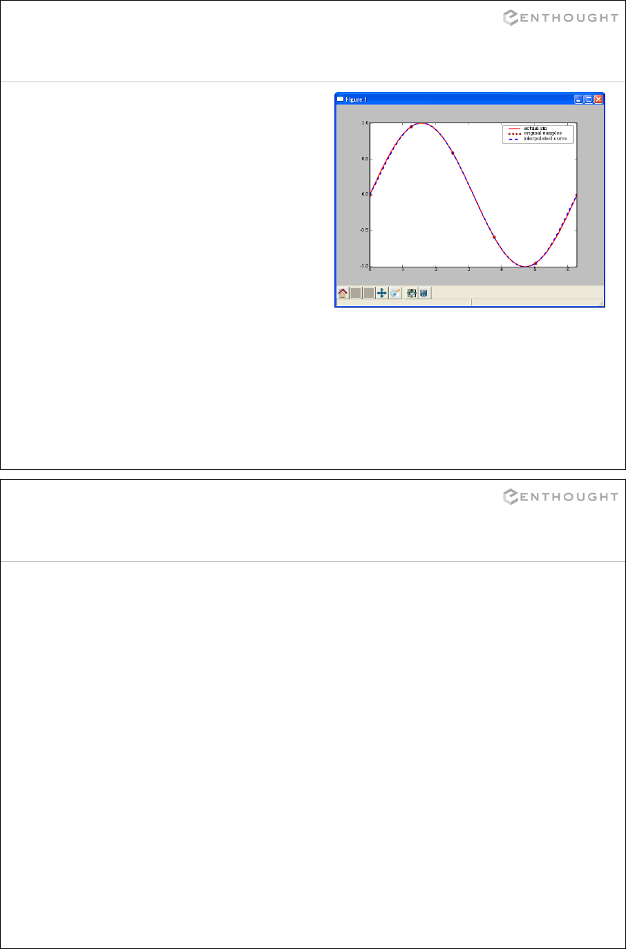
337
1D Spline Interpolation
# demo/interpolate/spline.py
from scipy.interpolate import interp1d
from pylab import plot, axis, legend
from numpy import linspace
# sample values
x = linspace(0,2*pi,6)
y = sin(x)
# Create a spline class for interpolation.
# kind='nearest' -> zeroth older hold.
# kind='linear' -> linear interpolation
# kind=n -> use an nth order spline
spline_fit = interp1d(x,y,kind=5)
xx = linspace(0,2*pi, 50)
yy = spline_fit(xx)
# display the results.
plot(xx, sin(xx), 'r-', x, y, 'ro', xx, yy, 'b--', linewidth=2)
axis('tight')
legend(['actual sin', 'original samples', 'interpolated curve'])
340
func = Rbf(x, y, …, function='multiquadric',
epsilon=None, smooth=0, norm=euclidean_norm)
Returns a function that uses interpolation to find the
value of new points.
•x – array of real values
•y – array of real values the same shape as x
•… - additional array arguments can be provided for N-d
interpolation
•function – basis function used to interpolate; one of
'multiquadric', 'inverse multiquadric', 'gaussian',
'linear', 'cubic', 'quintic', 'thin-plate'
•epsilon – adjustable constant for ’gaussian' or
'multiquadrics' functions. Defaults to approximate
average distance between nodes.
•smooth – Greater than zero increases smoothness of
approximation. Default of 0 is interpolation.
•norm – function (vectorized) that returns the distance
between two points
>>> from scipy.interpolate import Rbf
Radial Basis Functions
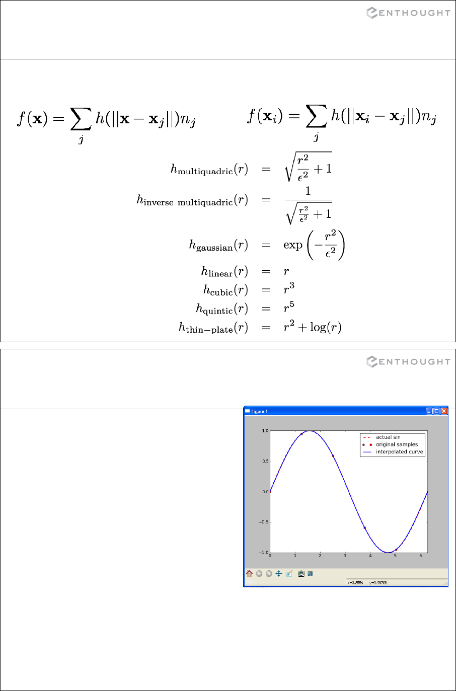
341
Radial Basis Functions
The function is approximated by a sum of radial functions with certain weights
nj:
Typical radial functions:
342
1D RBF Interpolation
# demo/interpolate/spline.py
from scipy.interpolate import Rbf
from pylab import plot, axis, legend
from numpy import linspace
# sample values
x = linspace(0,2*pi,6)
y = sin(x)
# Create a new function
fit = Rbf(x,y, function='gaussian')
xx = linspace(0,2*pi, 50)
yy = fit(xx)
# display the results.
plot(xx, sin(xx), 'r--', x, y, 'ro', xx, yy, 'b-', linewidth=2)
axis('tight')
legend(['actual sin', 'original samples', 'interpolated curve'])
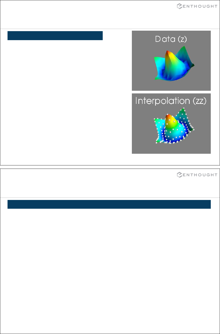
343
2D RBF Interpolation
EXAMPLE
>>> from scipy.interpolate import \
... Rbf
>>> from numpy import hypot, mgrid
>>> from scipy.special import j0
>>> x, y = mgrid[-5:6,-5:6]
>>> z = j0(hypot(x,y))
>>> newfunc = Rbf(x, y, z)
>>> xx, yy = mgrid[-5:5:100j,
-5:5:100j]
# xx and yy are both 2-d
# result is evaluated
# element-by-element
>>> zz = newfunc(xx, yy)
>>> from mayavi import mlab
>>> mlab.surf(x, y, z*5)
>>> mlab.figure()
>>> mlab.surf(xx, yy, zz*5)
>>> mlab.points3d(x,y,z*5,
scale_factor=0.5)
344
Optimization
Univariate Function Minimization
minimize_scalar - minimize a scalar-valued function of a single variable:
available methods include brent, bounded, golden
Multivariate Function Minimization (constrained and unconstrained)
minimize – minimize scalar-valued function of one or more variables: available
methods include BFGS, Nelder-Mead simplex, Newton conjugate gradient, COBYLA,
SLSQP, anneal, brute
Least Squares Fitting
leastsq - wrapper to the Fortran leastsq function from MINPACK
Curve Fitting
curve_fit – powerful, general, tool to fit functional parameters.
Root Finding
brentq, brenth, ridder, bisect, newton – find root of a scalar function
fixed_point – find the fixed point of a function
root – multidimensional root-finding: methods include hybr and lm for small problems
and krylov, brodyen2, and anderson for large problems.
scipy.optimize — Minimization and Root Finding
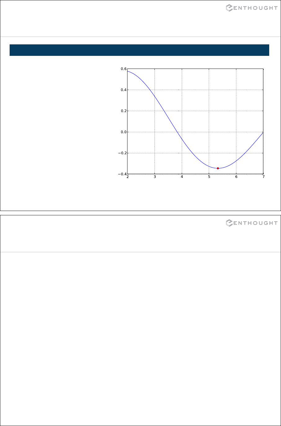
345
Optimization: 1-D Minimization
# minimize 1st order Bessel
# function between 4 and 7
>>> from scipy.special import j1
>>> from scipy.optimize import \
... minimize_scalar
>>> x = np.linspace(2, 7, 200)
>>> j1x = j1(x)
>>> plot(x, j1x)
>>> result = minimize_scalar(j1,
... method="bounded",
... bounds=[4, 7])
>>> j1_min = j1(result.x)
>>> plot(result.x, j1_min,'ro')
EXAMPLE: MINIMIZE BESSEL FUNCTION
Result Object
346
Output of minimize, minimize_scalar, and root is a Result object
with attributes:
x : solution to the optimization
success : True/False – did the optimization succeed?
status : integer termination status
message : termination status message
fun, jac, hess : values of the function, Jacobian,
Hessian, (if available) at the
optimized value
nfev, njev, nhev : number of evaluations of the
function, Jacobian, or Hessian (if available)
... : other attributes are added by
specific methods
Note: older legacy functions (fmin, fmin_bgfs, fminbound, fsolve, etc.) do not have a
unified API and are replaced by the above.
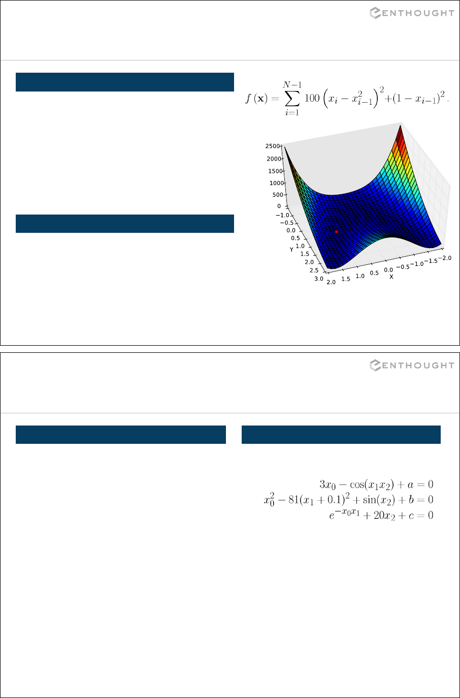
347
Optimization: Using Derivatives
Rosenbrock function
>>> from scipy.optimize import rosen_der
>>> result = minimize(rosen, x0,
... jac=rosen_der)
>>> print result.x
[ 1. 1. 1. 1. 1.]
>>> print result.nfev, result.njev
66 66
minimize: USING DERIVATIVE
minimize: WITHOUT DERIVATIVE
>>> from scipy.optimize import rosen
>>> x0 = [1.3, 1.6, -0.5, -1.8, 0.8]
>>> result = minimize(rosen, x0)
>>> print result.x
[ 1. 1. 1. 1. 1.]
>>> print result.nfev
462
348
Optimization: Solving Nonlinear Equations
>>> def equations(x,a,b,c):
... x0, x1, x2 = x
... eqs = \
... [3 * x0 - cos(x1*x2) + a,
... x0**2 - 81*(x1+0.1)**2 + sin(x2) + b,
... exp(-x0*x1) + 20*x2 + c]
... return eqs
>>> from scipy.optimize import root
# coefficients
>>> a = -0.5 ; b = 1.06
>>> c = (10 * pi - 3.0) / 3
# Optimization start location.
>>> initial_guess = [0.1, 0.1, -0.1]
# Solve the system of non-linear equations.
>>> result = root(equations, initial_guess, args=(a, b, c))
>>> print “root:”, result.x
root: [ 0.5 0. -0.52]
>>> print “solution at root:”, result.fun
solution at root: [ 0. -0. 0.]
SYSTEM OF EQUATIONS ROOT
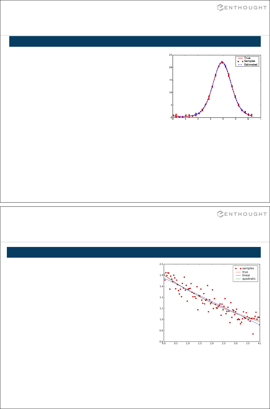
349
Optimization: Data Fitting
>>> from scipy.optimize import curve_fit
>>> from scipy.stats import norm
# Define the function to fit.
>>> def function(x, a, b, f, phi):
... result = a * exp(-b * sin(f * x + phi))
... return result
# Create a noisy data set.
>>> actual_params = [3, 2, 1, pi/4]
>>> x = linspace(0,2*pi,25)
>>> exact = function(x, *actual_params)
>>> noisy = exact + 0.3*norm.rvs(size=len(x))
# Use curve_fit to estimate the function parameters from the noisy data.
>>> initial_guess = [1,1,1,1]
>>> estimated_params, err_est = curve_fit(function, x, noisy, p0=initial_guess)
>>> estimated_params
array([3.1705, 1.9501, 1.0206, 0.7034])
# err_est is an estimate of the covariance matrix of the estimates
# (i.e. how good of a fit is it)
>>> err_est.diagonal()
array([ 0.0572, 0.006362, 0.0005834, 0.008979])
NONLINEAR LEAST SQUARES CURVE FITTING
350
Fitting Polynomials (NumPy)
>>> from numpy import polyfit, poly1d
>>> from scipy.stats import norm
# Create clean data.
>>> x = linspace(0, 4.0, 100)
>>> y = 1.5 * exp(-0.2 * x) + 0.3
# Add a bit of noise.
>>> noise = 0.1 * norm.rvs(size=100)
>>> noisy_y = y + noise
# Fit noisy data with a linear model.
>>> linear_coef = polyfit(x, noisy_y, 1)
>>> linear_poly = poly1d(linear_coef)
>>> linear_y = linear_poly(x)
# Fit noisy data with a quadratic model.
>>> quad_coef = polyfit(x, noisy_y, 2)
>>> quad_poly = poly1d(quad_coef)
>>> quad_y = quad_poly(x)
POLYFIT(X, Y, DEGREE)

351
Data Analysis with
Pandas
352
Pandas (version 0.12.0, Jul 2013) is a library to make analysis of structured datasets easy.
Author: Wes McKinney, http://pandas.pydata.org/
License: BSD
• New array-based data-structures with axis labeling + nice representation in ipython,
• Date/time management built-in, including timezones,
• Data alignment, data merging, data aggregation (group by), missing data management,
• Statistical tools (describe, moving stats, covariance, correlation, panel regression),
• Easy visualization (line plot, bar chart, boxplot, scatter plot matrix, ...) with Matplotlib.
•Built on top of: NumPy, pytables, matplotlib.
•Replaces scikits.timeseries. Is now an optional dependency of statsmodels.
•Offers similar features to larry, datarray (labeled arrays).
RELATED PROJECTS
GOALS
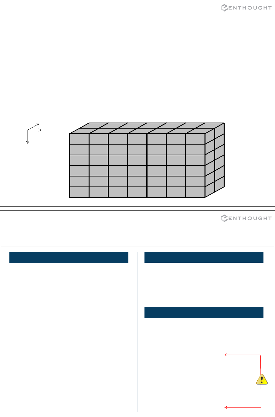
New Data Structures
353
PANDAs = PANel DAta = multi-dimensional data in stats & econometrics.
Data-structures:
•A Series is a 1D data-structure that derives from np.ndarray.
•A DataFrame is a 2D data-structure that can be viewed as a dictionary of series. It is NOT
a subclass of an numpy array.
•A Panel is a 3D data-structure that can be viewed as a dict of DataFrames.
index
columns
items
0
1
2
4
2
5
6
1
3
John
Jill
Chris
Dave
Ellen
Frank
1981
1975
NaN
1965
1973
1976
Doe
Ford
Jones
Smith
Frank
Hart
1
2
3
4
5
6
M
F
M
M
F
M
4.18
5.26
3.91
1.23
5.52
4.71
-1.18
1.26
0.91
NaN
0.52
-0.71
Rk, Fst N, Lst N, DoB Gend Grade offset
UT
TAMU
354
Creating (Time)Series
FROM LIST AND DICT
# Data and corresponding indices can
# be stored in lists.
>>> index = ['a', 'b', 'c', 'd']
>>> Series(range(4), index=index,
name='first series')
a 0
b 1
c 2
d 3
Name: first series
# data + indices in a dict
>>> d = {'a':0,'b':1,'c':2,'d':1}
>>> s = Series(d, name='first series')
>>> print s.name
'first series'
>>> s.name = ''
>>> print s.index
Index([a, b, c, d], dtype=object)
>>> print s.values, type(s.values)
array([0, 1, 2, 1], dtype=int64)
numpy.ndarray
>>> s.dtype
dtype('int64')
>>> from numpy.random import randn
>>> Series(randn(4), index=index)
a -1.062984
b -0.961625
c -0.720323
d 1.100681
FROM A NUMPY ARRAY
ACCESS ELEMENTS
# Access elements like an array
>>> s[2]
2
>>> s[:2]
a 0
b 1
# Access elements like a dictionary
>>> print s['c'], 'c' in s
2 True
# Slicing works on indices!
>>> s['a':'c']
a 0
b 1
c 2

355
Creating DataFrames
FROM A DICT OF SERIES
# DF from a dict of series: keys are
# column names.
>>> s2=Series(randn(3), name='B',
index=index[1:])
>>> d = {'A':s, 'B':s2}
>>> df = DataFrame(d)
A B
a 0 NaN
b 1 -0.961625
c 2 -0.720323
d 1 1.100681
>>> df.index, df.columns
Index([a, b, c, d], dtype=object)
Index([A, B], dtype=object)
>>> df.shape, df.dtypes
(4,2)
A int64
B float64
>>> df.values
array([[ 0. , nan],
[ 1. , -0.96162549],
[ 2. , -0.72032263],
[ 1. , 1.100680533]])
>>> DataFrame(randn(4,4), index=index,
columns=['A','B','C','D'])
A B C D
a 0.28164 -0.36826 0.04011 1.25030
b -0.71049 -1.23956 -0.08504 -0.08336
c -1.29446 0.70709 1.39642 0.49035
d 0.74632 -0.03512 -0.69237 0.81488
# List(series) interpreted as an array
>>> df2 = concat([s,s2], axis=1,
keys=['A', 'B'])
FROM A NUMPY ARRAY
ACCESS OR ADD ELEMENTS
>>> col1 = df['A']
>>> col2 = df.B
>>> df['flag'] = df['B'] > 0
>>> df.ix['c']
A 2
B -0.7203226
flag False
Name: c
>>> df.ix['c','B']
-0.7203226322119064
356
Creating Panels
FROM A DICT OF DATAFRAMES
# Panel from a dict of dataframes:
# keys used for third 'items' axis.
>>> df2=df.ix[::2,:]
>>> data = {'item1': df,'item2': df2}
>>> wp = Panel(data)
>>> wp.items, wp.major_axis,
wp.minor_axis
Index([item1, item2], dtype=object)
Index([a, b, c, d], dtype=object)
Index([A, B, flag], dtype=object)
>>> wp.shape
(2, 4, 3)
>>> wp.values
array([[[0, nan, False],
[1, -0.96162549, False],
[2, -0.72032263, False],
[1, 1.100680533, True]],
[[0.0, nan, False],
[nan, nan, nan],
[2.0, -0.72032263, False],
[nan, nan, nan]]],
dtype=object)
>>> items = ['foo','bar','baz','biz']
>>> Panel(randn(4,4,4), items=items)
<class 'pandas.core.panel.Panel'>
Dimensions: 4 (items) x 4 (major) x 4
(minor)
Items: foo to biz
Major axis: 0 to 3
Minor axis: 0 to 3
FROM A NUMPY ARRAY
ACCESS OR ADD ELEMENTS
>>> df1 = wp['item1']
A B flag
a 0 NaN False
b 1 -0.9616255 False
c 2 -0.7203226 False
d 1 1.100681 True
>>> df2 = wp.item2
>>> del wp['item1']
>>> wp.ix['item2','c','A']
2.0

357
Pandas IO
Format Method, Function, Class
txt, csv read_table, read_csv
clipboard read_clipboard
pickle read_pickle
HDF5 read_hdf, HDFStore
Excel read_excel, ExcelFile
R pandas.rpy.common.load_data
READING FUNCTIONS EXAMPLES
# Pickle is supported
>>> df.to_pickle('foo.pickle')
>>> read_pickle('foo.pickle')
# To load a table from an ascii file
df = read_table('foo.txt', sep=',',
header=1, skiprows=2, index_col=0,
names=['Paris', 'NY', 'Tokyo',
'London'], parse_dates=True,
na_values = [-9999])
# Long term storage: HDF5
>>> st = HDFStore('foo.h5')
>>> st['data1'] = df
>>> st['ser1'] = s
>>> s2 = st['ser1']
>>> st.close()
Format Method, Function, Class
txt, csv to_string, to_csv
html to_html
pickle to_pickle
HDF5 to_hdf, HDFStore
Excel to_excel, ExcelWriter
WRITING FUNCTIONS
Indexes and data alignment
358
ALIGNMENT FROM OPERATIONS
# Operations automatically align on
# the index (different from ndarray)
>>> s[1:] + s[:-2]
a NaN
b 1
c 2
d NaN
e NaN
RE-INDEXING
# reindex shuffles the existing index
>>> s.reindex(['c', 'b', 'a', 'e'])
c 2
b 1
a 0
e NaN
# The index attr can be overwritten
>>> s.index = ['p', 'q', 'r', 's']
# ‘rename’ modifies index label
>>> s.rename(lambda a: a.upper())
P 0
Q 1
R 2
S 3
# Sort by values
>>> s.values[:] = [5, 3, 0, 2]
>>> s.order()
r 0
s 2
q 3
p 5
# Explicit alignment of BOTH series
>>> s, s2 = s.align(s2)
# Sort a DF by a (list of) column(s)
>>> df.sort('A')
A B flags
a 0 NaN False
b 1 -0.961625 False
d 1 1.100681 True
c 2 -0.720323 False

More on indexing
359
INDEX TO/FROM A COLUMN
# Any dataframe column can become the
# index
>>> df
A B
a 0 NaN
b 1 -0.961625
c 2 -0.720323
d 3 1.100681
>>> df2 = df.set_index('A')
B
A
0 NaN
1 -0.961625
2 -0.720323
3 1.100681
# The opposite operation converts the
# index to a column
>>> df2.reset_index()
A B
0 0 NaN
1 1 -0.961625
2 2 -0.720323
3 3 1.100681
REDUNDANT INDEXES
# Although dangerous, it is possible
# to have redundant indices
>>> index = ['a', 'b', 'c', 'c']
>>> s=Series(range(4), index=index)
a 0
b 1
c 2
c 3
>>> s['c']
c 2
c 3
>>> type(s['c'])
pandas.core.series.Series
Multi-indexed pandas
360
MULTI-INDEXING SERIES MULTI-INDEXING DATAFRAMES
>>> df = DataFrame(randn(4,2),
index=ind)
0 1
bar one 0.24 0.81
two -0.96 0.49
baz one 1.23 0.29
two -0.97 1.18
>>> df.ix['bar']
0 1
one 0.24 0.81
two -0.96 0.49
>>> df.ix['bar', 'one']
0 0.24
1 0.81
Name: one
# Partial slicing works!
>>> df.ix[('bar','two'):('baz','two')]
0 1
bar two -0.96 0.49
baz one 1.23 0.29
two -0.97 1.18
>>> ind1=['bar', 'bar', 'baz', 'baz']
>>> ind2=['one', 'two', 'one', 'two']
>>> ind = [ind1,ind2]
>>> s = Series(randn(4), index=ind)
bar one 0.03
two 0.80
baz one 0.56
two -2.08
>>> s.index
MultiIndex
[('bar', 'one') ('bar', 'two') ('baz',
'one') ('baz', 'two')]
>>> s['bar']
one 0.03
two 0.80
>>> s.reindex([('baz', 'two'),
('bar', 'one')])
baz two -2.08
bar one 0.03

Multi-indexed pandas II
361
MANIPULATING INDEXES
# By default each index is identified
# by a level 0 (outer), 1 (inner)
>>> s.swaplevel(0,1)
one bar 0.03
two bar 0.80
one baz 0.56
two baz -2.08
# reorder_levels generalizes that
>>> s.reorder_levels([1,0])
(...)
>>> s.index.names=['first','second']
>>> s
first second
bar one 0.03
two 0.80
baz one 0.56
two -2.08
>>> df.index.names=['first','second']
>>> df.xs("one", level="second")
0 1
first
bar 0.24 0.81
baz 1.23 0.29
SLICING
>>> s.sortlevel(level='second')
bar one 0.03
baz one 0.56
bar two 0.80
baz two -2.08
SORTING
Computation with pandas
362
SERIES
# Series are subclasses of ndarrays:
# computations are element by element
>>> i = ['a', 'b', 'c', 'd']
>>> s = Series(range(4), index=i)
>>> s + 1
a 1
b 2
c 3
d 4
# All Numpy operators can be applied
>>> s2 = np.exp(s)
>>> s = s.astype(np.float32)
# including fancy indexing with masks
>>> s[s > 1.5] = 1.5
>>> df
A B flags
a 0 NaN False
b 1 -0.9 False
c 2 -0.7 False
d 1 1.1 True
# Dataframe computations are applied
# columns by columns
>>> df2 = df + 1
# Adding a series or re-scaling
>>> row = df.ix[1]
>>> df - row
A B flag
a -1 NaN False
b 0 0 False
c 1 0.2 False
d 0 2.0 True
# This would have been equivalent
>>> rescaled = df.sub(row, axis=0)
# Adding another dataframe can be done
# with a filler.
>>> df1.add(df2, fill_value=0)
# ‘apply’ a custom function to columns
>>> f = lambda x: x.max() - x.min()
>>> df.apply(f, axis = 0)
A 2
B 2
C True
DATAFRAMES

Statistical Analysis
363
DESCRIPTIVE STATS
# Descriptive stats available:
# count, sum, mean, median, min, max,
# abs, prod, std, var, skew, kurt,
# quantile, cumsum, cumprod, cummax
# Stats on DF are column per column
>>> print df.mean(), df.mean(axis=1)
A 1.000000 a -0.354328
B -0.227542 b 0.500000
flag 0.250000 c 0.426559
d 1.033560
# Stats func accept a level as kw arg
# applicable for multi-index pandas
>>> df.describe()
A B
count 4.000000 3.000000
mean 1.000000 -0.227542
std 0.816497 1.162964
min 0.000000 -1.062984
25% 0.750000 -0.891653
50% 1.000000 -0.720323
75% 1.250000 0.190179
max 2.000000 1.100681
>>> pandas.rolling_<TAB>
CORRELATIONS & REGRESSION
>>> cov = df.cov()
>>> ts.corr(ts2, method='kendall')
0.066666666666666693
>>> ols(y = ts2, x = ts)
Formula: Y ~ <x> + <intercept>
Number of Observations: 20
Number of Degrees of Freedom: 2
R-squared: 0.9936
Adj R-squared: 0.9932
Rmse: 0.0582
F-stat(1,18): 2772.7496, p-value: 0.0
Degrees of Freedom: model 1, resid 18
(...)
For more stats, see statsmodels.
Dealing with missing data
364
FIND & REMOVE/REPLACE NaN
# Combining overlapping datasets with
# a priority
>>> df1 = DataFrame({
'A' : [1.,nan,3.,5.,nan],
'B' : [nan,2.,3.,nan,6.]})
>>> df2 = DataFrame({
'A' : [5.,2.,4.,nan,3.,7.],
'B' : [nan,nan,3.,4.,6.,8.]})
>>> df1.combine_first(df2)
A B
0 1 NaN
1 2 2
2 3 3
3 5 4
4 3 6
57 8
# More custom merging to be
# implemented using combine and a
# custom function
# A boolean mask with ‘null’ values:
# None, np.NaN, np.inf, -np.inf
>>> np.all(isnull(s) | s.notnull())
True
# Replace missing values manually
>>> s[isnull(s)] = 0.
# Automatic version with forward fill
>>> s.fillna(method='ffill')
# Inverse operation
>>> s[s == -9999] = np.nan
# Remove all entries w/ missing values
>>> df.dropna(how='all')
# Interpolation also removes NaN
>>> s.interpolate()
# If mostly missing data, convert to
# SparseSeries, SparseDataFrame, ...
# Only stores non-null values & loc
>>> print len(s), s.count(), s.nbytes
1000, 10, 8000
MERGING DATASETS
SPARSE DATASETS
>>> sp_s = s.to_sparse()
>>> print sp_s.nbytes
80

Pivot tables and reshaping
365
PIVOTING (UN-)STACKING
# Stacking a DF creates a
# series with multiple indexes made
# from the column names.
>>> s
a b
one 1 2
two 3 4
>>> stacked = s.stack()
one a 1
b 2
two a 3
b 4
# Opposite operation unstacks the
# last level by default. If more cplx
# DF, can specify a level to unstack
>>> stacked.unstack()
a b
one 1 2
two 3 4
>>> stacked.unstack(level=0)
one two
a 1 3
b 2 4
# Repeating columns can be viewed as
# an additional axis
>>> df
date variable value
0 2000-01-03 A 0.469112
1 2000-01-04 A -0.282863
2 2000-01-05 A -1.509059
3 2000-01-03 B -1.135632
4 2000-01-04 B 1.212112
5 2000-01-05 B -0.173215
>>> df.pivot(index='date',
columns='variable', values='value')
variable A B
date
2000-01-03 0.469112 -1.135632
2000-01-04 -0.282863 1.212112
2000-01-05 -1.509059 -0.173215
Pivot tables and reshaping II
366
PIVOT_TABLE
# Another way to reshape a DF and
# aggregate at the same time
>>> df
A B C D
0 foo one small 1
1 foo one large 2
2 foo one large 2
3 foo two small 3
4 foo two small 3
5 bar one large 4
6 bar one small 5
7 bar two small 6
8 bar two large 7
>>> table= df.pivot_table(values='D',
rows=['A', 'B'], cols=['C'],
aggfunc=np.sum)
>>> table
small large
foo one 1 4
two 6 NaN
bar one 5 4
two 6 7

Data aggregation
367
SPLIT WITH groupby
# Group data by one column’s value
>>> gps = df.groupby('flags')
# gps = iterator of tuples with
# group name and sub part of df
>>> gps.groups
{False: ['a', 'b', 'c'], True:
['d']}
# groupby can also take a custom
# function that acts on index labels
>>> df = df.reset_index()
>>> myfunc = lambda x: x%2 == 0
>>> gps2 = df.groupby(myfunc)
# Series can also be grouped by
>>> df['A'].groupby(myfunc)
# which is identical to
>>> gps2['A']
Aggregation in a dataset is done in 3 steps: Split > Apply > Combine
APPLY WITH aggregate()
# Values in groups can be aggregated
>>> gps.sum()
A B
flags
False 3 -1.6
True 1 1.1
# Version more flexible but slower
>>> gps.aggregate(np.sum)
# agg is even more flexible
>>> gps.agg([np.mean, np.std])
>>> gps.agg({'A':'sum', 'B':'std'})
A B
flags
False 3 0.141421
True 1 NaN
# Values in groups can be
# transformed (length conserved)
>>> f = lambda x: x - x.mean()
>>> gps.transform(f)
A B
a -1 NaN
b 0 -0.1
c 1 0.1
d 0 0.0
# Computations from values in
# groups can be turned into a DF
# of calcs
>>> desc = lambda x: x.describe()
Data aggregation II
368
APPLY WITH apply()
>>> gps['A'].apply(desc).unstack()
count mean std min 25% 50% 75% max
flags
False 3 1 1 0 0.5 1 1.5 2
True 1 1 NaN 1 1.0 1 1.0 1
>>> def f(group):
return DataFrame({'original':group,
'demeaned': group - group.mean()})
>>> gps['A'].apply(f)
demeaned original
index
a -1 0
b 0 1
c 1 2
d 0 1
APPLY WITH transform()

Dealing with date & time
369
CREATING DATE/TIME INDEXES UP-/DOWN-SAMPLING
>>> ts.resample('T')
2000-01-01 00:00:00 0
2000-01-01 00:01:00 NaN
2000-01-01 00:02:00 NaN
2000-01-01 00:03:00 1
2000-01-01 00:04:00 NaN
2000-01-01 00:05:00 NaN
2000-01-01 00:06:00 2
2000-01-01 00:07:00 NaN
2000-01-01 00:08:00 NaN
2000-01-01 00:09:00 3
Freq: T
# Group hourly data into daily
>>> ts2 = Series(randn(72), index=r)
>>> ts2.resample('D', how='mean’,
closed='left', label='left')
01-Jan-2000 0.397501
02-Jan-2000 0.186568
03-Jan-2000 0.327240
Freq: D
>>> my_avg = lambda x: x[1:-1].mean()
>>> ts3=ts2.resample('D', how=my_avg)
# The index can be a list of
# dates+times locations that can be
# automatically generated
>>> date_range('1/1/2000',periods=4)
<class
'pandas.tseries.index.DatetimeIndex'>
[2000-01-01 00:00:00, ..., 2000-01-04
00:00:00]
Length: 4, Freq: D, Timezone: None
# Specify frequency: us,ms,S,T,H,D,B,
# W,M,3min, 2h20min, 2W,...
>>> r=date_range('1/1/2000',periods=72,
freq='H')
>>> i=date_range('1/1/2000',periods=4,
freq=datetools.YearEnd())
>>> i=date_range('1/1/2000',periods=4,
freq=’3min’)
>>> ts=Series(range(4), index=i)
2000-01-01 00:00:00 0
2000-01-01 00:03:00 1
2000-01-01 00:06:00 2
2000-01-01 00:09:00 3
Freq: 3T
Dealing with date & time II
370
RANGES OF PERIODS CONVERT TIMESTAMP<->PERIOD
>>> ts = ps.to_timestamp(how='end')
2000-01-31 0
2000-02-29 1
2000-03-31 2
2000-04-30 3
Freq: M
>>> all(ts.to_period() == ps)
True
# The index can be a list of
# dates/times intervals
>>> PeriodIndex(['2011-1', '2011-2',
'2011-3', '2011-4'], freq='M')
<class 'tseries.period.PeriodIndex'>
freq: M
[Jan-2011, ..., Apr-2011]
length: 4
# They can be automatically generated
>>> pr = period_range('1/1/2000',
periods=4, freq='M')
freq: M
[Jan-2000, ..., Apr-2000]
length: 4
>>> ps=Series(range(4), index=pr)
2000-01 0
2000-02 1
2000-03 2
2000-04 3
Freq: M, dtype: int64
TIMEZONES
# Timestamps/pandas can be tz aware
>>> ts_utc = ts.tz_localize('UTC')
>>>
ts_us=ts_utc.tz_convert('US/Eastern’)
2012-01-30 19:00:00-05:00 -0.425792
2012-02-28 19:00:00-05:00 0.788903
2012-03-30 20:00:00-04:00 0.009502
2012-04-29 20:00:00-04:00 1.775263
2012-05-30 20:00:00-04:00 -1.656727
Freq: M
>>> ts.index == ts_us.index
True
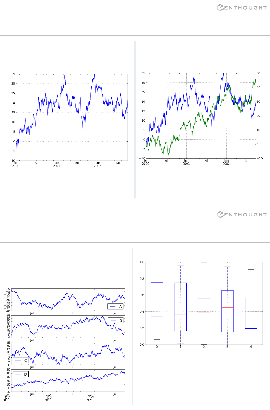
Visualizing (Time)series
371
>>> ts.plot()
See also
tools.plotting.lag_plot,
tools.plotting.autocorrelation_plot
>>> ts2.plot(secondary_y=True,
style='g')
372
>>> df.boxplot()
See also:
plot with kind=‘bar’,‘barh’, ‘kde’ keywd
hist method
tools.plotting.scatter_matrix,
andrews_curves, lag_plot
Visualizing DataFrames
>>> plt.figure()
>>> df.plot(subplots=True)
>>> plt.legend(loc='best')

373
Software Craftsmanship
in Python
374
Software Engineering Quotes
Programs should be written for people to read, and
only incidentally for machines to execute.
Structure and Interpretation of Computer Programs
Harold Abelson and Gerald Sussman

375
Software Engineering Quotes
You need to have empathy not just for your users, but
for your readers. It's in your interest, because you'll be
one of them. Many a hacker has written a program
only to find on returning to it six months later that he
has no idea how it works.
Hackers and Painters
Paul Graham
376
Software Engineering Quotes
Debugging is twice as hard as writing the code
in the first place. Therefore, if you write the
code as cleverly as possible, you are, by
definition, not smart enough to debug it.
Brian Kernighan
co-author of “The C Programming Language”
377
Useful References
or
378
Useful References
379
Software Carpentry
Software Carpentry
http://software-carpentry.org
A Python-based course
on software design and
engineering for
scientists.
380
Coding Modes
Interactive Mode: Quick Iteration
Interactive Prompt and exploratory development.
Production Mode: Building for the Ages
Creating code that will be re-used by you or
others.
The mode (context) you’re in changes
the way you code.

381
Naming Variables
Goal: Clarity for future readers of
the code
382
Typical Scientific Naming Convention
SUBROUTINE CFFTB1 (N,C,CH,WA,IFAC)
DIMENSION CH(*) ,C(*) ,WA(*) ,IFAC(*)
NF = IFAC(2)
NA = 0
L1 = 1
IW = 1
DO 116 K1=1,NF
IP = IFAC(K1+2)
L2 = IP*L1
IDO = N/L2
IDOT = IDO+IDO
IDL1 = IDOT*L1
IF (IP .NE. 4) GO TO 103
IX2 = IW+IDOT
IX3 = IX2+IDOT
IF (NA .NE. 0) GO TO 101
CALL PASSB4 (IDOT,L1,C,CH,WA(IW),WA(IX2),WA(IX3))
GO TO 102
<and on and on for 368 lines...>
STRAIGHT FROM FFTPACK

383
Primary Naming Consideration
POOR NAME CHOICES
# Update Cash Balance after stock trade.
c1 = n * ip
c2 = c1 + compute_tc(ins, n)
b -= c2
Priority 1: A variable name should fully and
accurately describe the entity and variable it
represents.
DESCRIPTIVE NAME CHOICES
# Update Cash Balance after stock trade.
instrument_cost = instrument_quantity * instrument_price
trade_cost = instrument_cost + transaction_cost(instrument_name,
instrument_quantity)
cash_balance -= trade_cost
384
Descriptive Name Choices
Entity Represented Variable Name
The number of trading
days in the current month
number_of_trading_days_in_current_month,
NumberOfTradingDaysPerMonth,
trading_days_in_current_month
Length of a moving
average window
length_of_moving_average_window,
lengthOfMovingAverageWindow
Risk Free Interest Rate risk_free_interest_rate
risk_free_rate
RiskFreeRate
These names are descriptive without much room for ambiguity, and
they are trivially decoded.
385
But the Names are Looooong…
Yes they are… Here are examples from the VTK library, a 3D
visualization tool set with 1800+ classes. (www.vtk.org)
386
The Downside to Long Names
# Long names can make simple formulas difficult to read,
# reducing clarity.
historic_daily_percent_price_change_per_day = \
(historic_daily_adjusted_close_price[1:] - \
historic_daily_adjusted_close_price[:-1]) \
/ historic_daily_adjusted_close_price[:-1]
DETAILED NAMES AND OBFUSCATED EQUATIONS
# Variable table:
# adj_close – Daily adjusted closing price for an instrument.
# change_percentage – Daily percent change in adjusted closing price.
change_percentage = (adj_close[1:] - adj_close[:-1]) / adj_close[:-1]
SHORTER NAMES IMPROVE EQUATION READABILITY

387
Optimal Name Lengths
Studies on debugging COBOL indicate*
10-16 character names is optimal length.
8-20 characters is almost as good.
* Gorla, N., A. C. Benander, and B. A. Benander. 1990. “Debugging Effort Estimation Using Software
Metrics.” IEEE Transactions on Software Engineering SE-16, no. 2 (February): 223-231
risk_free_interest_rate
length_of_moving_average_window
TOO LONG TOO SHORT JUST_RIGHT
r, rfir, rate
N, nw
risk_free_rate,
rsk_fr_rate
win_len, window_length,
Nwindow, mov_avg_win_len
388
Strategies for Shortening Names
Use Standard Abbreviations
administrator_information -> admin_info
Truncate consistently after 2nd or 3rd letter of each word
display_window -> dis_win
Remove Non-leading Vowels
risk_free_interest_rate -> rsk_fr_intrst_rt
Use only significant words in variable
start_of_next_paragraph -> next_paragraph_start
Remove useless suffixes
checking_account -> check_account
Iterate until variables are between 8 and 20 characters.

389
Using
extremely
short names
# This is ok.
for i in range(10):
scores[i] = 0
# But this is better.
for event in range(10):
decathalon_scores[event] = 0
LOOP INDICES I, J, and K
390
Using
extremely
short names
# Quick, what does each variable stand for?
y = a * sin(w*t + phi)
INDUSTRY STANDARD VARIABLES IN “SMALL” CONTEXT

391
Using
extremely
short names
def sin_wave(t, a=1, w=2*pi, phi=0):
"""
Return a sin wave form for time t.
Inputs
------
t: time in seconds
a: amplitude scale factor
w: frequency in radians/second
phi: phase shift in radians
Returns
-------
y: sin wave output
"""
y = a * sin(w*t + phi)
return y
INDUSTRY STANDARD VARIABLES IN “SMALL” CONTEXT
392
Domain vs. Computing Names
Variable names should relate to the problem space, not
generic programming terminology.
# Not so good… Algorithm-centric names
sum = 0
for record in record_list:
sum += will_retire(record.name)
# Better. Domain specific names.
gold_watch_order = 0
for employee in employee_list:
gold_watch_order += will_retire(employee.name)

393
Qualified Names
Use the “most important” part of the name as
the first word for “grouped” variables.
Usually, this is a noun.
MOST IMPORTANT WORD FIRST
# The _avg suffix on the price
# variable indicates it is an
# average price.
price_avg = mean(prices)
price_std = std(prices)
volume_avg = mean(volumes)
volume_std = std(volumes)
# But... Placing avg as a prefix
# read more like english
# (adjective first). So,
# arguments can be made for this
# approach as well.
avg_price = mean(prices)
avg_volume = mean(volumes)
std_price = std(prices)
std_volume = std(volumes)
ADJECTIVE FIRST AS IN ENGLISH
394
Qualified Names
Both prefixes and suffixes are found in “real” code, and
are quite readable.
Stick with one approach for a given variable group.
EXAMPLE WITH MIXED PREFIX AND SUFFIX VARIABLES
# Find the total profit made from group of trades.
profit_total = 0.0
current_trade_index = 0
while current_trade_index < last_trade_index:
current_trade = trades[current_trade_index]
profit, open_positions = update_positions(current_trade,
open_positions)
profit_total += profit
current_trade_index += 1

395
Global “Constants”
ENUMERATED TYPE PREFIX
# Type prefixes (like JOIN) often
# indicate a group of enumerated
# constants.
>>> constants.JOIN_BEVEL
1
>>> constants.JOIN_MITER
2
# wxPython is a GUI library
# wrapped around the C++
# wxWdigets library.
>>> import wx
# In C++, the constant is
# wxALIGN_CENTER
>>> wx.ALIGN_CENTER
2304
CONSTANTS IN MODULES GLOBALS
# "Constant" Global variables
# are often capitalized.
>>> from enthought.kiva import \
... constants
>>> constants.ITALIC
2
# But not always.
# [This is a global type.]
>>> import numpy
>>> numpy.float32
<type 'numpy.float32'>
The prefix used to differentiate constants
in other languages are often removed and
put in a single module in Python.
Note that these global values
are not truly constants as they
are writable variables.
396
Boolean Variables
# These common names are more
# informative.
done = True
found = True
success = True
valid = True
error = True
ok = True
# Using the prefix is_ can
# help identify booleans.
is_done = True
GENERIC NAMES
STANDARD NAMES
# Try not to use generic names
# as they don’t provide much
# information
flag = True
status = True
# Positive values are easy to
# interpret
if found:
employee_of_month = employee
# Negative Booleans take more
# mental gymnastics to read
if not not_found:
employee_of_month = employee
POSITIVE VALUES

397
Naming Containers
When naming lists (or sequences) of elements, use the plural
of the word, or a suffix that indicates it is a container.
# Using the _list suffix is descriptive and is more
# easily differentiated from a single item.
for name in name_list:
print name
VARIABLE SUFFIX FOR CONTAINERS
# Using the plural version of the variable is also a common paradigm.
for name in names:
print name
# For long variables names, the singular and plural approach isn’t
# as good. It is to hard to differentiate between the two.
close_price = {}
for equity_symbol in equity_symbols:
close_price[equity_symbol] = lookup_daily_close(equity_sybmol)
# And this is obviously problematic...
for moose in moose:
moose.bellow()
PLURAL VARIABLE NAME FOR CONTAINERS
398
Naming Variables Review
Priority 1: A variable’s name should fully and
accurately describe the entity and variable it
represents.
Names should refer to the real-world problem
rather than to computer programming terms.
A name should be long enough so that you
don’t have to puzzle out its meaning.
Short names are OK for industry standard
names, indices, and in “small” contexts.
Computed-value qualifiers should be at the end
of the name.

399
Documenting Code
400
Documentation Layers
API Documentation
Doc-strings for functions,
classes, and modules
Developer Documentation
Architecture Description,
Concepts, Developer Tutorials
Inline Code Comments
Describe intent of code
or algorithm design
Self Documenting Code
Variable and Function Names,
Good Design, Clear Layout
Application Documentation
End User Manuals,
Domain specific Tutorials, etc.
# Snippet out of a draw() method for drawing
# “bulls eye” cross hairs at the mouse position
# on a plot.
plot = self.component
if plot is None:
return
# sx, sy: mouse position in screen space.
sx, sy = plot.map_screen(self.current_position)
if plot.orientation == "h" and sx is not None:
self._draw_vertical_line(gc, sx)
elif sy is not None:
self._draw_horizontal_line(gc, sy)
if self.show_marker:
self._draw_marker(gc, sx, sy)
SELF DOCUMENTING CODE

401
Documentation Layers
API Documentation
Doc-strings for functions,
classes, and modules
Developer Documentation
Architecture Description,
Concepts, Developer Tutorials
Inline Code Comments
Describe intent of code
or algorithm design
Self Documenting Code
Variable and Function Names,
Good Design, Clear Layout
Application Documentation
End User Manuals,
Domain specific Tutorials, etc.
# Code snippet out of a Enthought Envisage
# library written by Martin Chilvers.
def unregister_services(self):
""" Unregister any service offered by the
plugin.
"""
# Services must be unregistered in reverse
# order that they were registered in.
service_ids = self._service_ids[:]
service_ids.reverse()
app = self.application
for service_id in service_ids:
app.unregister_service(service_id)
# Reset services in case the plugin is
# started again.
self._service_ids = []
INLINE CODE COMMENTS
402
Documentation Layers
API Documentation
Doc-strings for functions,
classes, and modules
Developer Documentation
Architecture Description,
Concepts, Developer Tutorials
Inline Code Comments
Describe intent of code
or algorithm design
Self Documenting Code
Variable and Function Names,
Good Design, Clear Layout
Application Documentation
End User Manuals,
Domain specific Tutorials, etc.
def interp(x, xp, fp, left=None, right=None):
"""
One-dimensional linear interpolation.
Returns the one-dimensional piecewise
linear interpolant to a function with
given values at discrete data-points.
Parameters
----------
x : array_like
The x-coordinates of the
interpolated values.
xp : 1-D sequence of floats
The x-coordinates of the data
points, must be increasing.
<snip>
Returns
-------
y : {float, ndarray}
Interpolated values, same shape as `x`.
<snip>
"""
API DOCUMENTATION [FROM NUMPY]
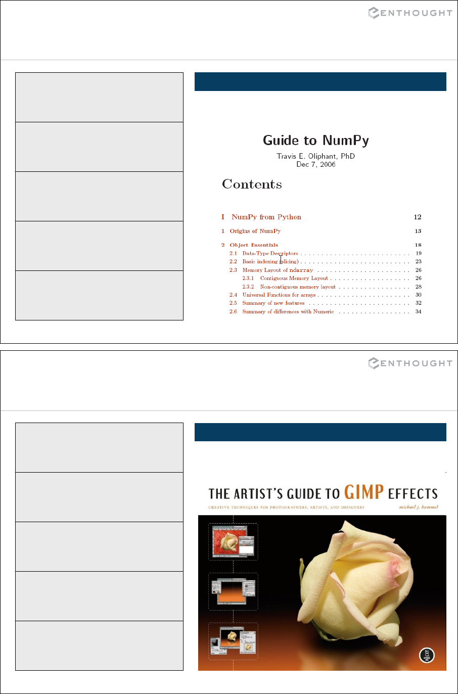
403
Documentation Layers
API Documentation
Doc-strings for functions,
classes, and modules
Developer Documentation
Architecture Description,
Concepts, Developer Tutorials
Inline Code Comments
Describe intent of code
or algorithm design
Self Documenting Code
Variable and Function Names,
Good Design, Clear Layout
Application Documentation
End User Manuals,
Domain specific Tutorials, etc.
DEVELOPER DOCUMENTATION
Provides a high level explanation of
concepts and use of a library.
404
Documentation Layers
API Documentation
Doc-strings for functions,
classes, and modules
Developer Documentation
Architecture Description,
Concepts, Developer Tutorials
Inline Code Comments
Describe intent of code
or algorithm design
Self Documenting Code
Variable and Function Names,
Good Design, Clear Layout
Application Documentation
End User Manuals,
Domain specific Tutorials, etc.
APPLICATION DOCUMENTATION

405
Documentation Layers
API Documentation
Doc-strings for functions,
classes, and modules
Developer Documentation
Architecture Description,
Concepts, Developer Tutorials
Inline Code Comments
Describe intent of code
or algorithm design
Self Documenting Code
Variable and Function Names,
Good Design, Clear Layout
Application Documentation
End User Manuals,
Domain specific Tutorials, etc. •Writing useful inline code
comments
•Creating function, class, and
module level documentation.
OUR FOCUS
406
Bad Code Comments
This comment is not even accurate. It
likely got out of sync with the code when
the bank implemented a minimum balance
policy and the comment wasn’t updated.
# Flag withdrawals that cause
# customer balance to become
# negative.
new_balance = balance - withdrawal
if new_balance < min_allowed_balance:
success = False
REPEATING THE CODE INCORRECT COMMENTS
Comments that just parrot code are
pretty much useless.
# Check if the printer is ready.
if printer_status == 'ready':
document.print()

407
Better Code Comments
Summarizing a few lines with a description
of the code’s intent is useful.
# Solve the dense linear system
# ZI=V for the currents I, given
# the impedance matrix Z and the
# driving voltage V.
lu_matrix, pivot = lu_factor(Z)
I = lu_solve((lu_matrix, pivot), V)
SUMMARY COMMENTS
Flag design decisions and trade-offs that
others should be aware of when editing
code in the future.
# FIXME: Sales tax hard coded to
# 8.25%. This should be passed in
# or looked up with a function
# call.
price_total = price * (1.0825)
FIXME COMMENTS
408
Function Docstring Format
""" Short docstring for the module goes here.
A longer description for the module goes it here. It
is typically multiple lines long.
"""
class Foo(object):
""" Short docstring for Foo class.
Longer docstring describing the Foo class.
"""
def some_method(self):
""" Short description for some_method.
Longer description for some_method...
"""
pass
def bar():
""" Short docstring for bar function.
And, not surprisingly, the long description for the function.
"""
pass
TYPICAL DOCUMENTATION FORMAT – FOO.PY
See the foo.py example in
the demo/docstrings
directory.

409
Command line help
In [12]: import foo
In [13]: foo?
Type: module
Base Class: <type 'module'>
String Form: <module 'foo' from 'foo.py'>
Namespace: Interactive
File: c:\temp\foo.py
Docstring:
Short docstring for the module goes here.
A longer description for the module goes here. It
is typically multiple lines long.
IPYTHON HELP PRINTS DOCSTRINGS
411
Styles of Documentation
Use simple docstrings for simple functions.
# from the Python standard library: locale.py
def str(val):
"""Convert float to integer, taking the locale into account."""
return format("%.12g", val)
SIMPLE IS AS SIMPLE DOES
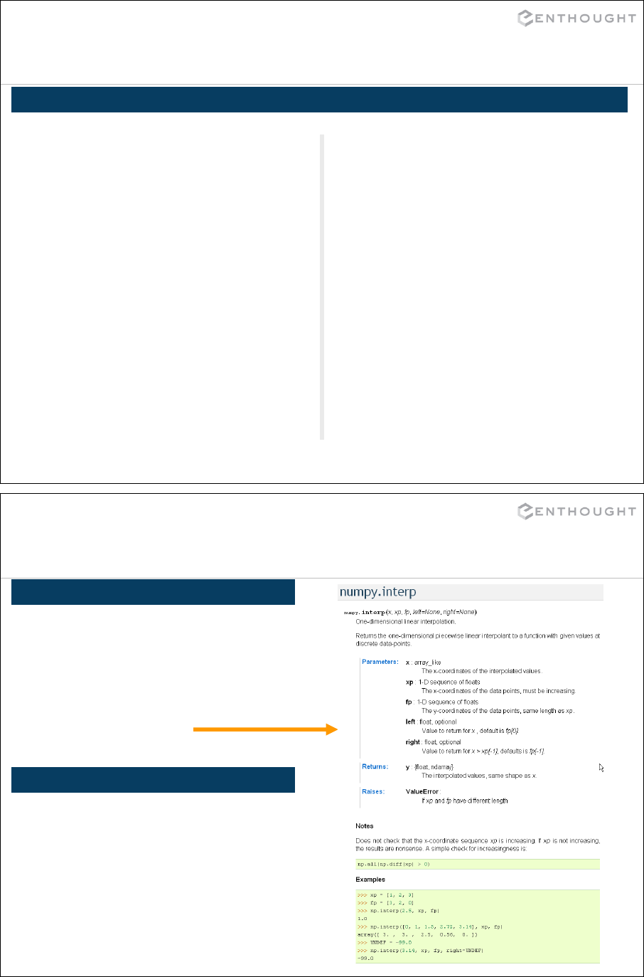
412
Styles of Documentation
FORMAL DOCUMENTATION SPECIFICATION
def interp(x, xp, fp, left=None, right=None):
"""
One-dimensional linear interpolation.
Returns the one-dimensional piecewise linear
interpolant to a function with given values
at discrete data-points.
Notes
=====
Does not check that the x-coordinate sequence
C{xp} is increasing. If C{xp} is not increasing,
the results are nonsense. A simple check for
increasingness is::
np.all(np.diff(xp) > 0)
Examples
========
>>> xp = [1, 2, 3]
>>> fp = [3, 2, 0]
>>> np.interp(2.5, xp, fp)
1.0
>>> np.interp([0, 1, 1.5, 2.72, 3.14], xp, fp)
array([ 3. , 3. , 2.5, 0.56, 0. ])
>>> UNDEF = -99.0
>>> np.interp(3.14, xp, fp, right=UNDEF)
-99.0
@param x : array_like.
The x-coordinates of the interpolated values.
@param xp : 1-D sequence of floats.
The x-coordinates of the data points, must be
increasing.
@param fp : 1-D sequence of floats.
The y-coordinates of the data points, same length
as C{xp}.
@param left : float, optional.
Value to return for C{x < xp[0]}, default is
C{fp[0]}.
@param right : float, optional.
Value to return for C{x > xp[-1]}, defaults is
C{fp[-1]}.
@return: float or ndarray.
The interpolated values, same shape as C{x}.
@raise ValueError: if C{xp} and C{fp} have different
lengths
"""
413
Formal Specifications
BENEFITS
•Formalism helps developers know
what to document.
•Uniform look to documentation.
•Tools like Sphinx and Epydoc can
generate nice HTML and PDF docs
automatically.
DRAWBACKS
•Can add (significant) overhead for
creating new functions.
•Overhead can inhibit developers
from re-factoring and creating new
functions when they should.

417
Restructured Text Docstring Format
http://epydoc.sourceforge.net/othermarkup.html#restructuredtext
http://docutils.sourceforge.net/docs/user/rst/quickstart.html
__docformat__ = "restructuredtext"
def interp(x, xp, fp, left=None, right=None):
"""
One-dimensional linear interpolation.
Returns the one-dimensional piecewise linear
interpolant to a function with given values at
discrete data-points.
:Parameters:
x : array_like.
The x-coordinates of the interpolated
values.
xp : 1-D sequence of floats.
The x-coordinates of the data points, must
be increasing.
fp : 1-D sequence of floats.
The y-coordinates of the data points, same
length as C{xp}.
left : float, optional.
Value to return for C{x < xp[0]}, default
is C{fp[0]}.
right : float, optional.
Value to return for C{x > xp[-1]}, defaults
is C{fp[-1]}.
:return: float or ndarray.
The interpolated values, same shape as C{x}.
:raises ValueError: if C{xp} and C{fp} have different
lengths
Notes
=====
Does not check that the x-coordinate sequence C{xp} is
increasing. If C{xp} is not increasing, the results
are nonsense. A simple check for increasingness is::
np.all(np.diff(xp) > 0)
Examples
========
>>> xp = [1, 2, 3]
>>> fp = [3, 2, 0]
>>> np.interp(2.5, xp, fp)
1.0
>>> np.interp([0, 1, 1.5, 2.72, 3.14], xp, fp)
array([ 3. , 3. , 2.5, 0.56, 0. ])
>>> UNDEF = -99.0
>>> np.interp(3.14, xp, fp, right=UNDEF)
-99.0
"""
418
Tips for Restructured Text
EXAMPLE CODE
Precede by '::' and a blank line.
""" Decorator to turn a code-
block inside of a function
into a string::
@func2str
def code():
c = a + b
d = a - b
"""
Result:
Decorator to turn a code-block inside of a
function into a string.
@func2str
def code():
c = a + b
d = a -b
PARAMETER DESCRIPTIONS
Parameter lists are “definition lists”, so every
item must have a separate description line.
x_ctrl : float
X-value of the control point.
y_ctrl : float
Y-value of the control point.
Not this ("unexpected indentation" error):
x_ctrl : float
y_ctrl : float
The control point.
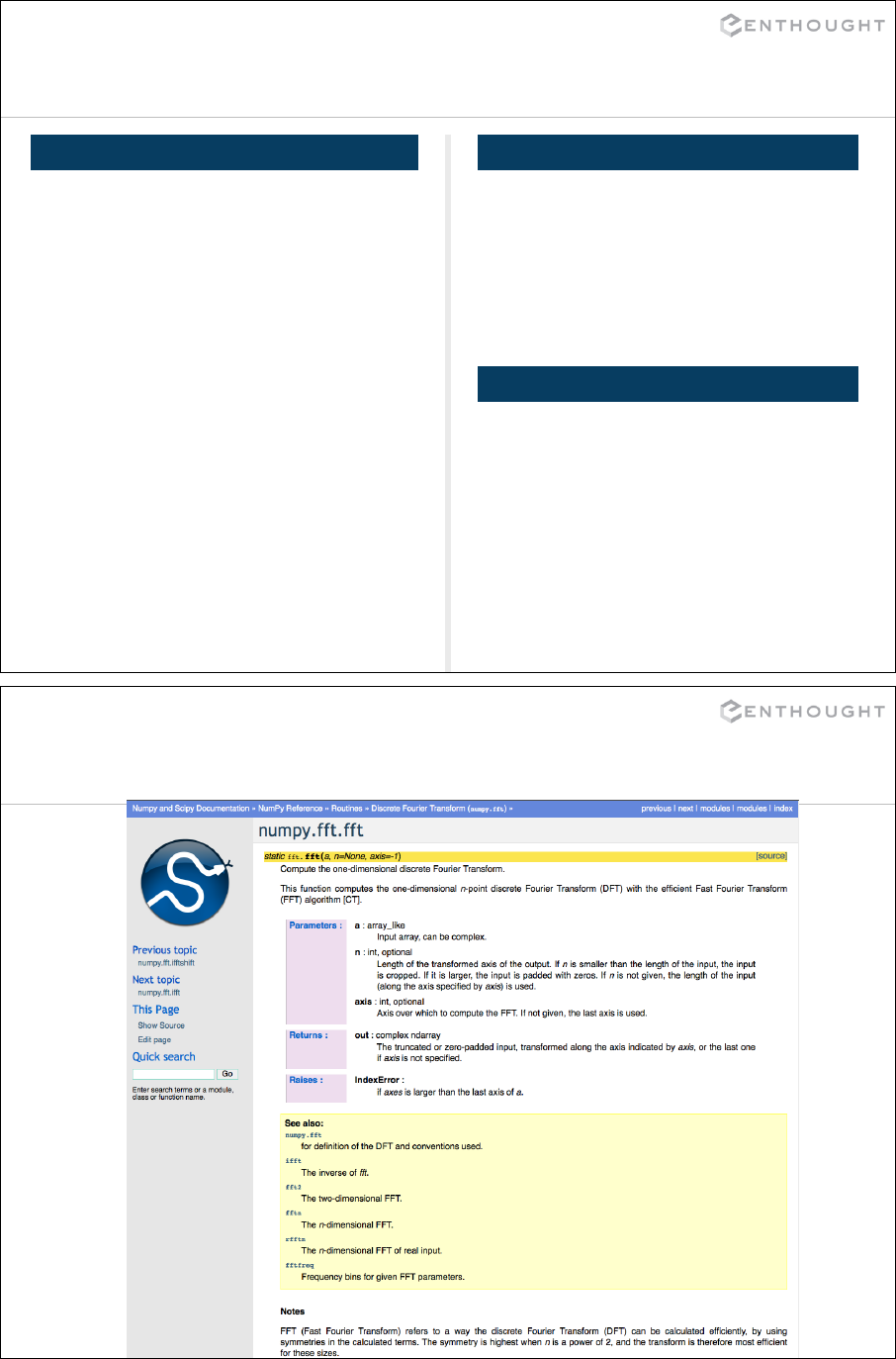
419
Tips for Restructured Text
This example looks nice in the source file,
but it is mixing syntax for bullet lists and
definition lists. It gets an indentation error.
- object: The value is treated
as a normal Python
object and is not
modified.
- file: The value is a file,
and supports various
types of conversions.
This can be made into valid ReST as a
bullet list or as a definition list.
- object: The value is treated
as a normal Python object and
is not modified.
- file: The value is a file,
and supports various types of
conversions.
MIXING LIST SYNTAX BULLET LISTS
object
The value is treated as a
normal Python object and is
not modified.
file
The value is a file, and
supports various types of
conversions.
OBJECT LISTS
420
Result with Sphinx

Number for several Python projects using cloc: http://cloc.sourceforge.net/
Result: SciPy: 32%, NumPy: 39%, ETS: 38% 421
Line Count Metrics for Documentation
$ ./cloc-1.56.pl numpy_trunk/
1023 text files.
1006 unique files.
385 files ignored.
http://cloc.sourceforge.net v 1.56 T=7.0 s (96.4 files/s, 53083.3 lines/s)
--------------------------------------------------------------------------------
Language files blank comment code
--------------------------------------------------------------------------------
C 81 22565 41042 120573
Python 424 24915 54760 83183
C/C++ Header 93 3064 3082 10007
Cython 6 940 2422 1523
C++ 8 52 116 643
make 9 100 74 457
HTML 5 47 15 403
CSS 3 134 46 369
Fortran 77 22 11 65 298
Fortran 90 15 56 20 200
sed 1 0 12 140
Bourne Shell 7 22 23 92
Bourne Again Shell 1 13 12 87
--------------------------------------------------------------------------------
SUM: 675 51919 101689 217975
--------------------------------------------------------------------------------
~39 % Comments
PORTION OF CODE THAT SHOULD BE COMMENTS
422
Coding Standards

423
Foolish Consistencies…
A foolish consistency is the hobgoblin of little minds, adored by little
statesmen and philosophers and divines. With consistency a great soul has
simply nothing to do. He may as well concern himself with his shadow on the
wall. Out upon your guarded lips! Sew them up with packthread, do. Else if you
would be a man speak what you think to-day in words as hard as cannon balls,
and to-morrow speak what to-morrow thinks in hard words again, though it
contradict every thing you said to-day. Ah, then, exclaim the aged ladies, you
shall be sure to be misunderstood! Misunderstood! It is a right fool’s word. Is it
so bad then to be misunderstood? Pythagoras was misunderstood, and Socrates,
and Jesus, and Luther, and Copernicus, and Galileo, and Newton, and every
pure and wise spirit that ever took flesh. To be great is to be misunderstood.
From the essay “Self Reliance,” by Ralph Waldo Emerson
Quoted in “PEP 8: Style Guide for Python,”
by Guido Von Rossum and Barry Warsaw
424
Foolish Consistencies…
True. But this statement is too often
used to get rid of good consistencies.
Show your creativity and personal style in your
algorithms, not your code layout. Code consistencies
make sharing and debugging much more efficient.

425
Foolish Consistencies…
(1) When applying the rule would make the code less readable, even for
someone who is used to reading code that follows the rules.
[editorial addition: Think about others, not you.]
(2) To be consistent with surrounding code that also breaks it (maybe
for historic reasons) -- although this is also an opportunity to clean
up someone else's mess (in true XP style).
* http://www.python.org/dev/peps/pep-0008/
Ralph doesn’t differentiate between good and foolish
consistencies, but Guido does. From the Python Coding
Standard*:
[There are] two good reasons to break a particular [coding standard]
rule:
426
Python Coding Standard
The Python Coding Standard is defined in
Python Enhancement Proposal 8* (PEP-8).
* http://www.python.org/dev/peps/pep-0008/
427
Indentation and Spaces
Never mix tabs and spaces in a file.
The “Tab Nanny” tool shipped with Python can
check this.
# mixed.py
# This file contains tabs and spaces
def foo(a):
print 'tabs'
print 'spaces'
C:>c:\python25\lib\tabnanny.py mixed.py
mixed.py 5 " print 'spaces'\n"
INDENTATION TABS OR SPACES?
Always use 4 spaces to indent code
blocks.
def sum(a):
total = 0
for value in a:
total += a
return total
4 spaces each
Most editors (emacs, vim, etc.)
have a python mode that will
insert 4 spaces when you type
<tab>.
428
Line Lengths and Wrapping
80 CHARACTER LINES
Limit line lengths to 80 characters.
Emacs and many other editors wrap at 80 characters by default.
# Use ‘\’ at the end of lines to continue on the next line.
from numpy import array, sin, cos, allclose, zeros, ones, \
uint32, float32
# Code enclosed in () or [] or {} does not need the ‘\’.
if (instrument_volume > VOLUME_THRESHOLD and
instrument_price < PRICE_THRESHOLD):
<do something>
# Align function arguments with beginning of function args.
a, b = some_long_function_call_name(with_long_var1,
and_long_var2)
429
Line Spacing
CLASS METHODS TOP LEVEL FUNCTIONS/CLASSES
# Separate Top level functions
# and classes with two blank
# lines.
def add(a, b):
total = a + b
return total
class Person(object):
def __init__(self, first, last):
self.first = first
self.last = last
class City(object):
pass
def __init__(self, name, state):
self.name = name
self.state = state
2 blank lines
# Separate class methods by a
# single line
class Person(object):
def __init__(self, first, last):
self.name = name
def full_name(self):
return self.first + \
self.last
def __repr__(self):
string = "Person(%s)" % \
self.full_name
1 blank line
430
Line Spacing
ONE LINER FUNCTIONS GROUPING FUNCTIONS
# Extra blank lines may be used
# (sparingly) to separate groups
# of related functions.
#---------------------------------
# Math functions
#---------------------------------
def add(a, b):
total = a + b
return total
def subtract(a, b):
difference = a – b
return difference
#---------------------------------
# Name functions
#---------------------------------
def full_name(first, last):
full = first + last
return full
# Lines can be omitted between
# one-liner implementations (such
# as dummy functions).
def stub1():
pass
def stub2():
pass
def stub3():
pass
extra space

431
Line Spacing
FUNCTION BODIES
# Use blank lines (sparingly) in
# functions to indicate logical
# sections.
def blend_color_channel(c1, c2, alpha):
# Validation
if not 0 <= alpha <= 1.0:
raise ValueError, "bad alpha"
# Channel blending algorithm.
new_c = c1 * alpha + \
c2 * (1 - alpha)
return new_c
extra space
432
Imports
SEPARATE LINES
# Imports should usually be on
# separate lines.
# Like this.
import os
import sys
# NOT like this.
import os, sys
IMPORT FROM A MODULE
# It is OK (and encouraged) to have
# have items imported from a module
# on the same line.
from numpy import array, float32
AVOID IMPORT *
# Do not use import * except at
# the command prompt.
# Only at the command prompt...
from numpy import *

433
Imports
LOCATION IN FILE
# Imports should happen at the top
# of a file so that others can
# quickly see the dependencies for
# a module.
# foo.py
import os
import sys
def some_function():
pass
...
LOCAL IMPORTS
# It is OCCASIONALLY useful to break
# this rule to have “optional”
# dependencies in a module. Be
# careful about this.
#----------------------------------
# Statistical Functions
#----------------------------------
def mean(a):
...
def std(a):
...
#----------------------------------
# Statistical Plot Functions
#----------------------------------
def histogram_plot(a):
from pylab import plot
...
434
Imports
GROUPING IMPORTS
# PEP-8
# Group imports in the following
# order:
# 1. Standard library imports
# 2. Related 3rd party imports
# 3. Application specific imports
import os
import sys
import wx
import pricing_models
LOCAL IMPORTS
# At Enthought, we expand the number
# of groupings and label them.
# 1. Standard library imports
# 2. Math/science libraries
# 3. Related 3rd party imports
# 4. Enthought specific libraries
# 5. Application specific imports
# Standard Imports
import os
import sys
# Math Imports
from numpy import array
# 3rd Party Imports
import wx
# Enthought Imports
from enthought.traits.api import Int
# Application Imports
import pricing_models

435
Absolute Imports
USE ABSOLUTE IMPORTS
Example directory structure for Python
libraries.
C:/
python_library/
package/
__init__.py
some_module.py
another_module.py
tests/
test_some_module.py
test_another_module.py
# PEP-8
# Relative imports of intra-package
# imports are highly discouraged.
# Use absolute package path for
# all imports.
# File: another_module.py
# Recommended
from package.some_module import func
# Discouraged
from some_module import func
...
436
Avoid Extraneous White Space
INSIDE (), [], OR {}
# Yes
spam(ham[1], {eggs: 2})
# No
spam( ham[ 1 ], { eggs: 2 } )
BEFORE COMMAS AND COLONS
# Yes
if x == 4:
print x, y
# No
If x == 4 :
print x , y
FUNCTION CALLS
# Yes
spam(1)
# No
spam (1)
SLICING AND INDEXING
# Yes
dict['key'] = list[index]
# No
dict ['key'] = list [index]
AROUND ASSIGNMENT
# PEP-8 encourages the first
# Yes
# No extra space
x = 1
y = 2
long_variable = 3
# No
# Align '=' character
x = 1
y = 2
long_variable = 3

437
Whitespace
AROUND BINARY OPERATORS
# Binary operators are surrounded by
# a space on either side.
# Yes
if a > 1:
b = 2 * (a + 1)
# No
if a> 1:
b= 2 * (a+1)
FUNCTION ARGUMENTS
# Don’t put spaces around ‘=‘ in
# keyword arguments.
# Yes
def quad(x, a=0, b=1, c=0):
y = a * x**2 + b * x + c
return y
# No
def quad(x, a = 0, b = 1, c = 0):
y = a * x**2 + b * x + c
return y
438
Compound Statements
COMPOUND STATEMENTS
# Compound statements are discouraged
# Yes
if foo == 'blah':
do_something()
func1()
func2()
func3()
# No
if foo == 'blah': do_something()
func1(); func2(); func3();

439
Naming Conventions
VARIABLES GLOBAL VARIABLES
# Use lower_case notation without
# capital letters for variables in
# your functions, methods, and scripts.
# Yes
lower_case = 3
# No
CamelCase = 3
mixedCase = 3
Mixed_Case = 3
# Use UPPER_CASE notation for
# module level “constants” or
# “static” class variables.
# File: foo.py
# Globals
# Yes
UPPER_CASE = 3
# No
CamelCase = 3
mixedCase = 3
Mixed_Case = 3
def some_function(a):
result = a * UPPER_CASE
return result
440
Naming Conventions
FUNCTIONS AND METHODS
# function and methods should use
# lower_case names with underscores.
# Do not use the Java convention of
# mixedCase.
# Yes
def some_function(a):
pass
# No
def SomeFunction(a):
pass
def someFunction(a):
pass
CLASSES
# Class names are CamelCase.
# If there is one class in a file and
# class is named FooBar, the file is
# named foo_bar.
# file: foo_bar.py
# Yes
class FooBar(object):
def some_method(self):
pass
# No
class foo_bar(object):
def some_method(self):
pass

441
Naming Conventions
PRIVATE CLASSES AND FUNCTIONS
# Names of ‘private’ classes, methods
# and functions start with a single
# underscore.
def _private_function(a):
pass
def _PrivateClass(object):
pass
442
Naming Packages and Modules
MODULE NAMES
# Package directories should be all
# lower case alpha-numeric characters.
# Avoid underscores unless absolutely
# necessary.
# Yes
packagename
# No
PackageName
package_name
PACKAGE NAMES
# Module names should be lower case
# with underscores.
# Yes
foo_bar.py
# No
FooBar.py

443
Using Future
•division
In “old” Python, 1/2 would become 0 because it used “integer”
division. In Python 3.0, 1/2 will be 0.50.
•with_statement
Enable the with statement found in Python 2.5 and beyond.
•absolute_import
Distinguish between absolute and relative module imports.
import foo imports from the top level of the module namespace.
import .foo imports from the same package as this module.
Python can turn on planned features for future versions of Python that are
backward incompatible. Here are several commonly used future features:
from __future__ import division, absolute_import, with_statement
444
Using Future
All future_statements must appear near the top of the module. The
only lines that can appear before a future_statement are:
""" This is a module docstring.
"""
# This is a comment, preceded by a blank line and followed by
# a future_statement.
from __future__ import with_statement
from math import sin
from __future__ import division # compile-time error!
# ERROR because it is preceded by a non-future_statement.
The module docstring (if any).
Comments.
Blank lines.
Other future_statements.
FUTURE EXAMPLE

445
Common Directory Structure
PACKAGE/MODULE/TESTS LAYOUT
Example directory structure for Python libraries.
C:/
python_library/
yourpackage/
__init__.py
some_module.py
another_module.py
tests/
test_some_module.py
test_another_module.py
The tests for module have
are named similarly (test_
prefix) but live “one level
below” in a tests directory.
446
Functions and
Refactoring Code

448
Evolution of a script
EXPLORATORY SCRIPT
# Read data files into some structure.
for file in files:
...
# Check for errors in data.
if data > bad_value:
raise ValueError
...
# Execute one or more algorithms on the data.
important_number = data * 2 + blah...
...
# Create a report about the results.
print important_number
...
Useful software often starts its life as a script.
449
To A Function
ONE MEGA-FUNCTION TO BIND THEM ALL
def display_data_report(files):
# Read data files into some structure.
for file in files:
...
# Check for errors in data.
if data > bad_value:
raise ValueError
...
# Execute one or more algorithms on the data.
important_number = data * 2 + blah
...
# Create a report about the results.
print important_number
...
Evolves to a function…

450
Evolution Stops
MEGA-FUNCTION BENEFITS
And Stops…
There are some short term benefits to this.
•Easy (quick) to create from original script.
•Easy to read and modify during construction.
• All the code is “in one place.”
•Access to all variables at any time.
(Global namespaces are nice that way.)
•Achieves some re-use.
451
Evolution to a library
Long term benefits come from continuing to “refactor” function until there
is “one idea per function.”
def data_from_files(files):
# Read data files into a structure.
for file in files:
...
def check_for_errors(data):
# Check for errors in data.
if data > bad_value:
raise ValueError
...
def calc_important_number(data):
# Execute one or more algorithms.
important_number = data * 2
...
def create_report(data, calc_data):
# Create a report about results.
print important_number
...
LOW LEVEL FUNCTION LIBRARY DRIVER FUNCTIONS
def display_data_report(files):
"""
"Driver" function that calls
the low level library functions.
"""
data = data_from_files(files)
check_for_errors(data)
res = calc_important_number(data)
create_report(data, res)

452
“One Idea Per Function” Benefits
•Smaller, less complex snippets of code that are
easier for others (and you) to read code in the
future.
•Builds up a set of re-usable functions.
•Easier for others to modify behavior without
modifying original code.
•Better Potential for Testing.
453
Avoid Duplicate Code
DUPLICATED CODE
instrument1_prices = lookup_price(instrument1, start_date, stop_date)
instrument1_price_avg = mean(instrument1_prices)
print_summary(instrument1, instrument1_prices, instrument1_price_avg)
instrument2_prices = lookup_price(instrument2, start_date, stop_date)
instrument2_price_avg = mean(instrument2_prices)
print_summary(instrument2, instrument2_prices, instrument2_price_avg)
REFACTOR TO USE A FUNCTION
# refactor code so duplicated lines are in a function.
def summarize_price_info(instrument, start_date, stop_date):
instrument_prices = lookup_price(instrument, start_date, stop_date)
instrument_price_avg = mean(instrument_prices)
print_summary(instrument, instrument_prices, instrument_price_avg)
# Now call the function for the two different instruments.
summarize_price_info(instrument1, start_date, stop_date)
summarize_price_info(instrument2, start_date, stop_date)
454
Simplify Complex Conditionals
COMPLEX CONDITIONAL
if ( isinstance(float, value)
and sqrt(value**2+other_value**2) > 21
and value < 5):
do_something_important(value)
REFACTOR TO USE A FUNCTION
# Refactor code so the complex expression is in a function.
def is_important(value, other_value):
important = isinstance(float, value) \
and sqrt(value**2+other_value**2) > 21 \
and value < 5
return important
if is_important(value, other_value):
do_something_important(value)
455
Useful Reference

456
Testing Code
458
Test Driven Development
Overarching Concept:
Write Tests First.

459
Useful Reference
460
Test Driven Development
pt2 (x2, y2)
dy
dx
pt1 (x1, y1)
slope = dy/dx
PROBLEM DEFINITION
461
Test Driven Development
TEST
# test_fancy_math.py
from nose.tools import assert_almost_equal
from fancy_math import slope
def test_slope():
pt1 = [0.0, 0.0]
pt2 = [1.0, 2.0]
s = slope(pt1, pt2)
assert_almost_equal(s, 2)
pt2 (x2, y2)
dy
dx
pt1 (x1, y1)
slope = dy/dx
462
Test Driven Development
TEST
# test_fancy_math.py
from nose.tools import assert_almost_equal
from fancy_math import slope
def test_slope():
pt1 = [0.0, 0.0]
pt2 = [1.0, 2.0]
s = slope(pt1, pt2)
assert_almost_equal(s, 2)
FANCY_MATH
# Simplest function that passes, tests…
def slope(pt1, pt2):
return 2
pt2 (x2, y2)
dy
dx
pt1 (x1, y1)
slope = dy/dx

463
Test Driven Development
TEST
# test_fancy_math.py
from nose.tools import assert_almost_equal
from fancy_math import slope
def test_slope():
pt1 = [0.0, 0.0]
pt2 = [1.0, 2.0]
s = slope(pt1, pt2)
assert_almost_equal(s, 2)
FANCY_MATH
# Simplest function that passes, tests…
def slope(pt1, pt2):
return 2
pt2 (x2, y2)
dy
dx
pt1 (x1, y1)
slope = dy/dx
Smart Alec...
464
TDD Rationale
Build only the features you need.
(YAGNI Principle – you ain’t gonna need it)
All the features are tested.
You are the first consumer of your API.
(Helps in design process)

465
Running Nosetests
In [27]: ls
Volume in drive W is Shared Folders
Volume Serial Number is 0000-0064
Directory of w:\...\slope
09/29/2008 11:41 PM <DIR> .
09/29/2008 11:30 PM <DIR> ..
09/29/2008 11:37 PM 123 fancy_math.py
09/29/2008 11:41 PM 195 test_fancy_math.py
2 File(s)
2 Dir(s) 48,067,092,480 bytes free
In [28]: !nosetests -v
test_fancy_math.test_slope ... ok
-------------------------------------------------------------------
Ran 1 test in 0.000s
OK
FROM IPYTHON
466
Using Unittest Framework
# Test cases:
# - each method is a unit test
# - found by nosetests as well
from unittest import TestCase
from fancy_math import *
class TestModule(TestCase):
def test_slope(self):
pt1 = [0.0, 0.0]
pt2 = [1.0, 2.0]
s = slope(pt1, pt2)
self.assertAlmostEqual(s, 2)
TESTS EMBEDDED IN CLASSES

467
Doctests
def factorial(n):
"""
Return the product of all positive integers less than
or equal to n.
Example:
>>> factorial(3)
6
>>> factorial(4)
24
"""
if n <= 1:
result = 1
else:
result = n * factorial(n-1)
return result
if __name__ == "__main__":
import doctest
doctest.testmod()
TESTS EMBEDDED IN DOCSTRINGS
Optional
468
Monitoring execution

The logging module
•Key part of good software craftsmanship
•Part of the standard library
•Structure of a logging system:
1. Create a logger instance
2. Add 1 or more handlers (console, file, http, …)
3. Set a level for these handlers or the logger
4. [OPTIONAL] Control the formatting
5. Add logger calls throughout the code
469
Simple Example
from logging import getLogger, FileHandler, StreamHandler
logger = getLogger() # Root logger
console_handler = StreamHandler()
logger.addHandler(console_handler)
file_handler = FileHandler("log.txt”)
logger.addHandler(file_handler)
logger.debug("Debugging level message") # Hidden
logger.info("Informative level message") # Hidden
logger.warning("Warning level message")
Warning level message
logger.error("Error level message")
Error level message
470
More numerous
More critical

More complex example
from logging import getLogger, StreamHandler, DEBUG, INFO, WARNING, ERROR
from logging.handlers import RotatingFileHandler
logger = getLogger(__name__) # local file’s logger
console_handler = logging.StreamHandler()
logger.addHandler(console_handler)
# File handler that is a rotating file
file_handler = RotatingFileHandler("log.txt", maxBytes=1024, backupCount=3)
formatter = logging.Formatter("%(levelname)s - %(asctime)s - %(name)s "
"- %(message)s")
file_handler.setFormatter(formatter)
logger.addHandler(file_handler)
logger.setLevel(DEBUG) # highly sensitive logger
logger.debug("Debugging level message")
DEBUG - 2012-10-16 23:08:03,592 – package.analysis_module - Debugging level
message 471
Ways to time execution
Timing inside the code (Good)
•the time module from std lib
Timing in ipython (Better):
•%timeit “magic command”
•-t option of ‘run’ (optionally –N also)
Profiling the code (Best):
•cProfile or line_profiler package
472

Timing in python
473
USE TIME PACKAGE USE IPYTHON TOOLS
import time
from numpy.random import randn
from numpy import linspace, pi, exp, sin
from scipy.optimize import leastsq
def func(x,A,a,f,phi):
return A*exp(-a*sin(f*x+phi))
def errfunc(params, x, data):
return func(x, *params) - data
start = time.time()
params0 = [1,1,1,1]
x = linspace(0,2*pi,25)
ptrue = [3,2,1,pi/4]
true = func(x, *ptrue)
noisy = true + 0.3*randn(len(x))
pmin,ierr = leastsq(errfunc, params0,
args=(x, noisy))
print “Total: %f s” %(time.time()-start)
# For a script
>>> run –t [-N10] test.py
IPython CPU timings (estimated):
User : 1.10 s.
System : 0.00 s.
Wall time: 1.11 s.
# For a function call
>>> import random as rand
>>> import numpy.random as \
nprand
>>> %timeit rand.randint(0,10)
100000 loops, best of 3: 2.02 us
per loop
>>> %timeit nprand.randint(10)
10000000 loops, best of 3: 178 ns
per loop
474
Timing and Profiling Code

Ways to time execution
Timing inside the code (Good)
•the time module from std lib
Timing in ipython (Better):
•%timeit “magic command”
•-t option of ‘run’ (optionally –N also)
Profiling the code (Best):
•cProfile or line_profiler package
475
Timing in python
476
USE TIME PACKAGE USE IPYTHON TOOLS
import time
from numpy.random import randn
from numpy import linspace, pi, exp, sin
from scipy.optimize import leastsq
def func(x,A,a,f,phi):
return A*exp(-a*sin(f*x+phi))
def errfunc(params, x, data):
return func(x, *params) - data
start = time.time()
params0 = [1,1,1,1]
x = linspace(0,2*pi,25)
ptrue = [3,2,1,pi/4]
true = func(x, *ptrue)
noisy = true + 0.3*randn(len(x))
pmin,ierr = leastsq(errfunc, params0,
args=(x, noisy))
print “Total: %f s” %(time.time()-start)
# For a script
>>> run –t [-N10] test.py
IPython CPU timings (estimated):
User : 1.10 s.
System : 0.00 s.
Wall time: 1.11 s.
# For a function call
>>> import random as rand
>>> import numpy.random as \
nprand
>>> %timeit rand.randint(0,10)
100000 loops, best of 3: 2.02 us
per loop
>>> %timeit nprand.randint(10)
10000000 loops, best of 3: 178 ns
per loop

477
Profiling with cProfile
cProfile (and its pure python version, profile) are profiling tools in the standard
library.
The cProfile workflow has two main steps:
1. Run the code to be profiled via the cProfile’s run() (or runctx())
function or using the kernprof.py script. This counts and times function
calls, and generates a profiling dataset.
1. Process and display the profile data. In the simplest case (e.g.
cProfile.run('foo()')), a predefined report is generated and printed.
For finer control, you can save the raw data to a file and process it using the
pstats module.
WORKFLOW
Profiling with kernprof.py
478
From the command line (if the line_profiler package is installed):
$ kernprof.py datafit.py
Wrote profile results to datafit.py.prof
$ python -m pstats
Welcome to the profile statistics browser.
% read datafit.py.prof
datafit.py.prof% strip
datafit.py.prof% sort time
datafit.py.prof% stats 20
(...)
ncalls tottime percall cumtime percall
filename:lineno(function)
1 0.299 0.299 0.363 0.363 _core.py:4(<module>)
1 0.130 0.130 0.635 0.635 mpl.py:1(<module>)
1 0.115 0.115 0.482 0.482 __init__.py:14(<module>)
12 0.114 0.009 0.415 0.035 __init__.py:1(<module>)
(...)

479
Profiling from iPython
>>> import time
>>> def func(n):
... if n < 0:
... return
... time.sleep(0.1*n)
... func(n-1)
... return
...
>>> import cProfile
>>> cProfile.run('func(3)')
11 function calls (7 primitive calls) in 0.601 seconds
Ordered by: standard name
ncalls tottime percall cumtime percall filename:lineno(function)
5/1 0.000 0.000 0.601 0.601 <stdin>:1(func)
1 0.000 0.000 0.601 0.601 <string>:1(<module>)
1 0.000 0.000 0.000 0.000 {method 'disable' of …
4 0.600 0.150 0.600 0.150 {time.sleep}
EXAMPLE
480
Profiling with cProfile
OUTPUT TABLE COLUMNS
ncalls The number of calls. Counts of the form N/M indicate N actual calls
(including recursive calls), and M 'primitive' (nonrecursive) calls.
tottime The total time spent in the given function (and excluding time made in
calls to sub-functions).
percall The quotient of tottime divided by ncalls.
cumtime The total time spent in this and all subfunctions (from invocation until
exit). This figure is accurate even for recursive functions.
percall The quotient of cumtime divided by primitive calls.
filename:lineno(function)
Provides the respective data of each function.

481
Profiling with cProfile
USE PSTATS TO CONTROL THE TABLE
# Save the raw profile data to a file.
>>> cProfile.run('func(3)', filename='func.prof')
# Use pstats.Stats to manipulate the data.
>>> import pstats
>>> stats = pstats.Stats('func.prof')
# Clean up the filenames.
>>> stats.strip_dirs()
<pstats.Stats instance at 0xdbda0>
# Sort by the cumulative time.
>>> stats.sort_stats('cumulative')
<pstats.Stats instance at 0xdbda0>
# Print the table.
>>> stats.print_stats()
482
Profiling with cProfile
USE PSTATS TO CONTROL THE TABLE - CONTINUED
Wed May 4 14:56:13 2011 func.prof
11 function calls (7 primitive calls) in 0.600 seconds
Ordered by: cumulative time
ncalls tottime percall cumtime percall
filename:lineno(function)
1 0.000 0.000 0.600 0.600 <string>:1(<module>)
5/1 0.000 0.000 0.600 0.600 <stdin>:1(func)
4 0.600 0.150 0.600 0.150 {time.sleep}
1 0.000 0.000 0.000 0.000 {method 'disable' of …}
<pstats.Stats instance at 0xdbda0>

483
Profiling with cProfile
MORE OUTPUT CONTROL
Arguments to Stats.sort_stats(…)
Valid
Argument
Meaning
'calls'
call count
'cumulative'
cumulative
time
'file'
file name
'module'
file name
'pcalls
'
primitive
call count
'line'
line
number
'name'
function name
'nfl
'
name/file/line
'stdname
'
standard name
'time'
internal time
484
Profiling with cProfile
MORE OUTPUT CONTROL
Arguments to Stats.print_stats([restriction, …]) allow to filter the
output:
Each restriction is either:
•an integer to select the number of lines to output;
•a decimal fraction between 0.0 and 1.0 to select a percentage of lines; or
•a regular expression to match the filename.

485
Profiling with cProfile
A FEW USEFUL OUTPUT CASES
# Find out what is taking the most time:
>>> stats.sort_stats('cumulative').print_stats(10)
# Find functions in which the program is spending the
# the most time (not including calls to other functions):
>>> stats.sort_stats('time').print_stats(10)
# Check how often __init__ is called in all the modules
# (sorted by name):
>>> stats.sort_stats('file').print_stats('__init__')
486
Profiling with cProfile
Python standard library documentation:
•http://docs.python.org/library/profile.html
Doug Hellman's "Python Module of the Week" blog:
•http://blog.doughellmann.com/2008/08/pymotw-profile-cprofile-pstats.html
MORE DOCUMENTATION

487
line_profiler and kernprof
line_profiler and kernprof are profiling tools developed by Robert Kern.
•line_profiler is a module for doing line-by-line profiling of functions.
•kernprof is a convenient script for running either line_profiler or the standard
library's cProfile module.
$ easy_install line_profiler
1. Decorate the functions to be profiled with @profile.
2. Run your script using kernprof.py with the –l option. For example,
$ kernprof.py –l script_to_profile.py
3. Run the line_profiler module to display the results. For example,
$ python –m line_profiler script.to_profile.py.lprof
4. Adjust your code, and repeat steps 2-4.
5. Remove the @profile decorators.
INSTALLATION
TYPICAL WORKFLOW
488
line_profiler example
import re
PATTERN = r"https?:\/\/[\w\-_]+(\.[\w\-_]+)+([\w\-
\.,@?^=%&:/~\+#]*[\w\-\@?^=%&/~\+#])?"
@profile
def scan_for_http(f):
addresses = []
for line in f:
result = re.search(PATTERN, line)
if result:
addresses.append(result.group(0))
return addresses
if __name__ == "__main__":
import sys
f = open(sys.argv[1], 'r')
addresses = scan_for_http(f)
for address in addresses:
print address
http_search.py
See demo/profiling directory
for code.

489
line_profiler example
$ kernprof.py –l http_search.py sample.html
…
http://sphinx.pocoo.org/
Wrote profile results to http_search.py.lprof
$ python –m line_profiler http_search.py.lprof
Run kernprof.py and line_profiler
Timer unit: 1e-06 s
File: http_search.py
Function: scan_for_http at line 6
Total time: 0.016079 s
Line # Hits Time Per Hit % Time Line Contents
==============================================================
6 @profile
7 def scan_for_http(f):
8 1 3 3.0 0.0 addresses = []
9 1350 2080 1.5 12.9 for line in f:
10 1349 12417 9.2 77.2 result = re.search(PATTERN, line)
11 1349 1513 1.1 9.4 if result:
12 39 65 1.7 0.4 addresses.append(result.group(0))
13 1 1 1.0 0.0 return addresses
490
line_profiler example
import re
PATTERN = r"https?:\/\/[\w\-_]+(\.[\w\-_]+)+([\w\-
\.,@?^=%&:/~\+#]*[\w\-\@?^=%&/~\+#])?"
@profile
def scan_for_http(f):
addresses = []
pat = re.compile(PATTERN)
for line in f:
result = pat.search(line)
if result:
addresses.append(result.group(0))
return addresses
if __name__ == "__main__":
import sys
f = open(sys.argv[1], 'r')
addresses = scan_for_http(f)
for address in addresses:
print address
http_search2.py

491
line_profiler example
$ kernprof.py –l http_search2.py sample.html
…
Wrote profile results to http_search2.py.lprof
$ python –m line_profiler http_search2.py.lprof
Run kernprof.py and line_profiler on the modified file
Timer unit: 1e-06 s
File: http_search2.py
Function: scan_for_http at line 6
Total time: 0.00911 s
Line # Hits Time Per Hit % Time Line Contents
==============================================================
6 @profile
7 def scan_for_http(f):
8 1 3 3.0 0.0 addresses = []
9 1 3117 3117.0 34.2 pat = re.compile(PATTERN)
10 1350 1995 1.5 21.9 for line in f:
11 1349 2507 1.9 27.5 result = pat.search(line)
12 1349 1415 1.0 15.5 if result:
13 39 72 1.8 0.8 addresses.append(result.group(0))
14 1 1 1.0 0.0 return addresses
492
pdb
The Python debugger

493
What is pdb?
pdb is part of the standard library
pdb, like Python, is interactive and interpreted,
allowing for the execution of arbitrary Python
code in the context of any stack frame
pdb can debug a “post-mortem” condition, and
can also be called under program control
ipdb (not in std lib) is similar but includes tab
completion
494
Starting pdb
• Run the script from the command line under debugger control
C:\> python -m pdb script.py [arg ...]
•During an iPython session, here are some of the common pdb functions
used for debugging :
>>> pdb.run( statement )
Execute the statement (given as a string) under debugger control
>>> pdb.runcall( function[, argument, ...] )
Call the function (not a string) with the given arguments under debugger control
>>> pdb.pm()
Start the debugger at the point of the last exception
•Inside a script or a module to hard-code a breakpoint
import pdb ; pdb.set_trace()
•Useful for hard-coding a breakpoint in a program even if code is not being
debugged (analyzing a failed assertion, etc.)

495
pdb commands
•
pdb
runs as an interactive session having a specific set of commands
• Some of the more common
pdb
commands:
(Pdb) h(help)[command]
One of the most important! Lists all the commands available, or help on a
specific command
(Pdb) u(p) / d(own)
Pop up or push down the execution stack
(Pdb) b(reak)[[filename:]lineno | function[, condition]]
Set a breakpoint at a specific file/line or function and optionally if a specific
condition is met. If no args are given, list all the breakpoints & their numbers
(Pdb) s(tep) / n(ext)
Execute the current line only. step will push into a function call and next will
execute the function call and move to the next statement in the current function
(Pdb) a(rgs)
Print the args for the current function
496
pdb commands
(Pdb) l(ist) [first[, last]]
List the source code at the point of execution. Args first and last set a range
for the number of lines printed. No args prints 11 lines around the current
line, if only first, prints 11 lines around that line.
(Pdb) j(ump) lineno
Jump to a line in the bottom-most frame only and execute from there. Not all
jumps are possible!
(Pdb) p / pp [expression]
Print or “pretty print” expression in the context of the current frame
(Pdb) a(lias) [name [command]]
Create an alias for command named name, or list all aliases.
Here are two useful aliases (especially when placed in a .pdbrc file):
#print all instance variables (usage "pi classInst")
alias pi for k in %1.__dict__.keys(): print "%1.",k,"=",%1.__dict__[k]
#print instance variables in self
alias ps pi self
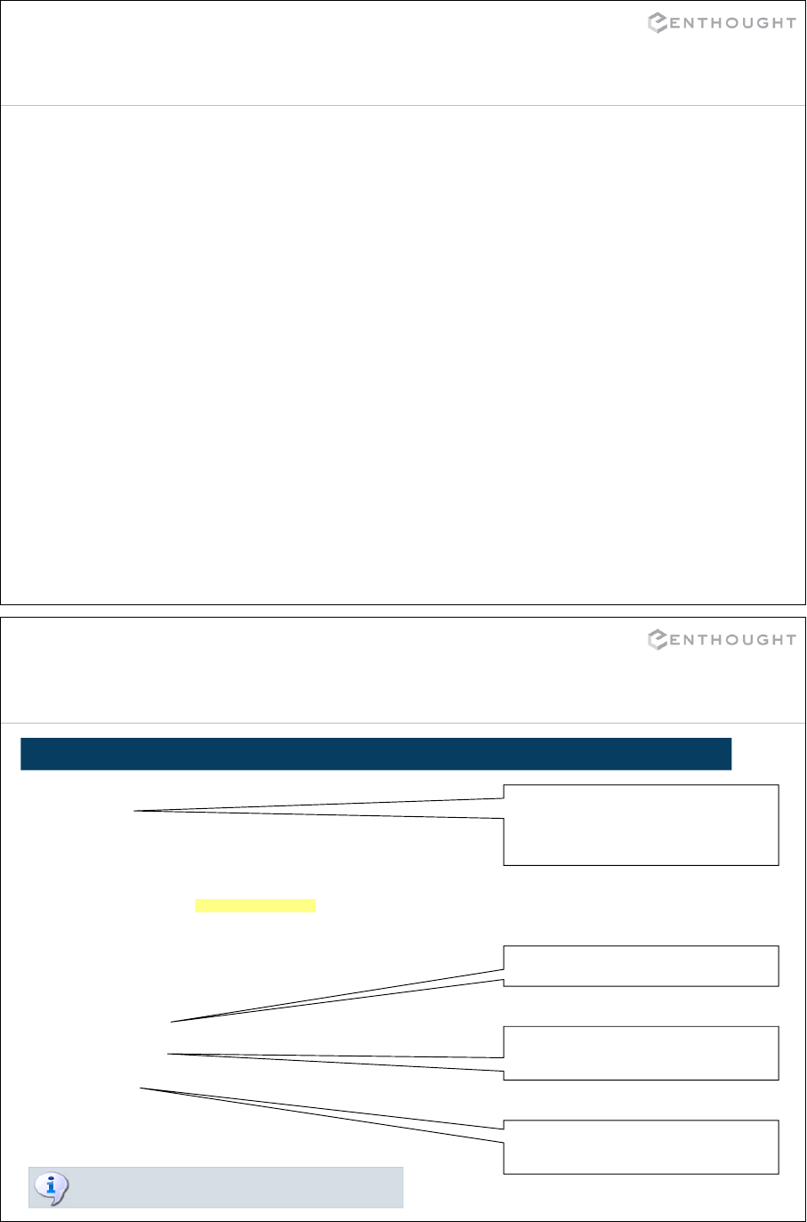
497
iPython and pdb
# ipython can call pdb automatically upon error
In [1]: pdb
Automatic pdb calling has been turned ON
In [2]: import middle
In [3]: middle.run()
---------------------------------------------------------------------------
IndexError Traceback (most recent call last)
Z:\projects\Training\pdb\<console>
Z:\projects\Training\pdb\middle.py in run()
31 """
32 for i in range( 1, 11 ) :
33 l = make_list( i )
---> 34 print "The middle item(s) in %s\n\tis/are %s\n" % (l, get_middle( l ))
35
Z:\projects\Training\pdb\middle.py in get_middle(item_list)
9
10 if( num_items % 2 ) :
---> 11 return item_list[half]
12
13 return item_list[(half - 1):(half + 1)]
IndexError: list index out of range
> z:\projects\training\pdb\middle.py(11)get_middle()
-> return item_list[half]
498
ipdb> l
6 """
7 num_items = len( item_list )
8 half = num_items * 2
9
10 if( num_items % 2 ) :
11 -> return item_list[half]
12
13 return item_list[(half - 1):(half + 1)]
14
15
16 def make_list( size=0 ) :
ipdb> item_list
['0']
ipdb> half
2
ipdb> c
In [4]:
Example session
DEBUGGING FROM ORIGIN OF EXCEPTION
Print the contents of the list
Print the value of the index
ah-ha!
Print the source code around
the line which raised the
exception
Test this with middle.py in Demos/pdb
Return to ipython

499
>>> import pdb
>>> import middle
>>> pdb.runcall( middle.run )
> z:\projects\pgtraining\pdb\middle.py(32)run()
-> for i in range( 1, 11 ) :
(Pdb) s
> z:\projects\pgtraining\pdb\middle.py(33)run()
-> l = make_list( i )
(Pdb) n
> z:\projects\pgtraining\pdb\middle.py(34)run()
-> print "The middle item(s) in %s\n\tis/are %s\n" % (l, get_middle( l ))
(Pdb) s
--Call--
> z:\projects\pgtraining\pdb\middle.py(2)get_middle()
-> def get_middle( item_list ) :
(Pdb) s
...
> z:\projects\pgtraining\pdb\middle.py(11)get_middle()
-> return item_list[half]
(Pdb) item_list
['0']
(Pdb) half
2
Example session
DEBUGGING MIDDLE.PY FROM THE START
Print the contents of the list
Print the value of the index
ah-ha!
We know make_list is ok, so
skip over it with “next”
Continue to execute lines
until we see something
suspicious
In Demos/ directory, file_sum.py contains a
class which computes the sum of every
number in a file.
file_sum.py has 2 bugs.
Once fixed, the script runs like this:
500
Debugging exercise
C:\> python file_sum.py dir.dat
The sum of all numbers in dir.dat is 4355

501
Other debugging tools
•ipdb (not in std lib) offers the same functionalities as pdb
(set_trace allowing to march through execution) but
allow more interactive exploration thanks to the tab
completion like in ipython. BUT still only allow 1 line
evaluations.
•To do more exploration at a given point in an
application, IPython can be invoked, with its embed
function:
from IPython import embed ; embed()
It starts a normal ipython session with the namespace
populated from the namespace of your application at the
break point. To exit, ctrl-d.
502
Python and Other Languages:
An Overview

503
Why use another language with Python?
•Best of both worlds: Tested and optimized legacy code +
flexibility of Python
•Python as glue: Combine several components into one
larger program
•Speedup Python: Speed up performance critical
components with a faster language
•Division of labor: Let Fortran be an array processing
DSL, let Python and its ecosystem handle automatic
testing, file IO, text processing, data munging, GUI
integration, HTTP serving, etc.
504
External language toolkit
Wrapping legacy code and external libraries:
•Wrap with hand-written extension module
•Cython wrap C/C++ with custom interface
•SWIG Automatically wrap large C/C++ libraries
•f2py Automatically wrap Fortran libraries
•ctypes Easy to manually wrap external libraries
Speed up Python code:
•Hand-written extension module
•Cython Add type information to Python
•Weave Speed up NumPy array expressions
•Shedskin and others not covered here

505
Wrapping and Levels of Granularity
Coarse-grained:
•Python communicates with external program via config files
and command line interface using subprocess
Medium-grained:
•In external program, create a handful of functions that are
designed to be wrapped with Python
•Wrap a select few pieces of external program and
customize the interface
Fine-grained:
•Wrap everything using automatic tool like SWIG or f2py.
•Expose the entire library and its API to Python.
506
Hand Wrapping C/C++

507
The Wrapper Function
#ifndef FACT_H
#define FACT_H
int fact(int n);
#endif
static PyObject* wrap_fact(PyObject *self, PyObject *args)
{
/* Python-C data conversion */
int n, result;
if (!PyArg_ParseTuple(args, "i", &n))
return NULL;
/* C Function Call */
result = fact(n);
/* C->Python data conversion */
return Py_BuildValue("i", result);
}
fact.h
WRAPPER FUNCTION
fact.c
#include "fact.h"
int fact(int n)
{
if (n <=1) return 1;
else return n*fact(n-1);
}
508
Complete Example
/* Must include Python.h before any standard headers! */
#include "Python.h"
#include "fact.h"
/* Define the wrapper functions exposed to Python (must be static) */
static PyObject* wrap_fact(PyObject *self, PyObject *args) {
int n, result;
/* Python->C Conversion */
if (!PyArg_ParseTuple(args, "i", &n))
return NULL;
/* Call our function */
result = fact(n);
/* C->Python Conversion */
return Py_BuildValue("i", result);
}
/* Method table declaring the names of functions exposed to Python */
static PyMethodDef ExampleMethods[] = {
{"fact", wrap_fact, METH_VARARGS, "Calculate the factorial of n"},
{NULL, NULL, 0, NULL} /* Sentinel */
};
/* Module initialization function called at "import example" */
PyMODINIT_FUNC initexample(void) {
(void) Py_InitModule("example", ExampleMethods); }

509
Compiling/using your extension
C:\...\> gcc –c fact.c fact_wrap.c –I. –Ic:\python27\include
C:\...\> gcc -shared fact.o fact_wrap.o -Lc:\python27\libs
-lpython27 -o example.pyd
BUILD DYNAMIC LIB BY HAND (EPD ON WINDOWS)
~\...\> gcc –c -fpic fact.c fact_wrap.c –I. –I/usr/include/python2.7
~\...\> gcc -shared fact.o fact_wrap.o -L/usr/lib/python2.7/config
-lpython2.7 -o example.so
BUILD BY HAND (UNIX)
Note that the include and library directories are platform specific. Also, be
sure to link against the appropriate version of Python (2.7 in these examples).
USING THE MODULE IN PYTHON
In [1]: import example
In [2]: dir(example)
Out[2]: ['__doc__', '__file__', '__name__', '__package__', ‘fact']
510
Building using setup.py
# setup.py files are the Python equivalent of Make
from distutils.core import setup, Extension
ext = Extension(name='example', sources=['fact_wrap.c', 'fact.c'])
setup(name="example", ext_modules=[ext])
SETUP.PY
# Build and install the module.
$ setup.py build
$ setup.py install
# Or build the module "in-place" to ease testing.
$ setup.py build_ext –inplace --compiler=mingw32
* Blue text needed only on windows.
CALLING SETUP SCRIPTS

More details
511
More details on the wrapping functions (C <-> Python):
http://docs.python.org/extending
More details on writing a setup.py file to incorporate
extension modules:
http://docs.python.org/extending/building.html
Using NumPy arrays in hand-wrapped C code:
http://docs.scipy.org/doc/numpy/reference/c-api.html
... and a simple example: demo/hand_wrap_ndarray/
512
Cython

513
What is Cython?
Cython is a Python-like language for writing extension modules. It allows
one to mix Python with C or C++ and significantly lowers the barrier to
speeding up Python code.
The cython command generates a C or C++ source file from a Cython
source file; the C/C++ source is then compiled into a heavily optimized
extension module.
Cython has built-in support for working with NumPy arrays and Python
buffers, making numerical programming nearly as fast as C and (nearly) as
easy as Python.
http://www.cython.org/
514
A really simple example
# Cython has its own "extension builder" module that knows how
# to build cython files into python modules.
from distutils.core import setup
from distutils.extension import Extension
from Cython.Distutils import build_ext
ext = Extension("pi", sources=["pi.pyx"])
setup(ext_modules=[ext],
cmdclass={'build_ext': build_ext})
See demo/cython for this example.
Build it using build.bat.
PI.PYX
# Define a function. Include type information for the argument.
def multiply_by_pi(int num):
return num * 3.14159265359
SETUP_PI.PY

515
A simple Cython example
$ python setup_pi.py build_ext --inplace -c mingw32
>>> import pi
>>> pi.multiply_by_pi()
Traceback (most recent call last):
File "<stdin>", line 1, in ?
TypeError: function takes exactly 1 argument (0 given)
>>> pi.multiply_by_pi("dsa")
Traceback (most recent call last):
File "<stdin>", line 1, in ?
TypeError: an integer is required
>>> pi.multiply_by_pi(3)
9.4247779607700011
CALLING MULTIPLY_BY_PI FROM PYTHON
516
(some of) the generated code
static PyObject *__pyx_f_2pi_multiply_by_pi(PyObject *__pyx_self,
PyObject *__pyx_args, PyObject *__pyx_kwds); /*proto*/
static PyObject *__pyx_f_2pi_multiply_by_pi(PyObject *__pyx_self,
PyObject *__pyx_args, PyObject *__pyx_kwds) {
int __pyx_v_num;
PyObject *__pyx_r;
PyObject *__pyx_1 = 0;
static char *__pyx_argnames[] = {"num",0};
if (!PyArg_ParseTupleAndKeywords(__pyx_args, __pyx_kwds, "i",
__pyx_argnames,
&__pyx_v_num)) return 0;
/* "C:\pi.pyx":2 */
__pyx_1 = PyFloat_FromDouble((__pyx_v_num * 3.14159265359));
if (!__pyx_1) {__
pyx_filename = __pyx_f[0]; __pyx_lineno = 2; goto __pyx_L1;}
__pyx_r = __pyx_1;
__pyx_1 = 0;
C CODE GENERATED BY CYTHON

517
Def vs. CDef
# Python callable function.
def inc(int num, int offset):
return num + offset
# Call inc for values in sequence.
def inc_seq(seq, offset):
result = []
for val in seq:
res = inc(val, offset)
result.append(res)
return result
DEF — PYTHON FUNCTIONS CDEF — C FUNCTIONS
INC FROM PYTHON
# inc is callable from Python.
>>> inc.inc(1,3)
4
>>> a = range(4)
>>> inc.inc_seq(a, 3)
[3,4,5,6]
# cdef becomes a C function call.
cdef int fast_inc(int num,
int offset):
return num + offset
# fast_inc for a sequence
def fast_inc_seq(seq, offset):
result = []
for val in seq:
res = fast_inc(val, offset)
result.append(res)
return result
FAST_INC FROM PYTHON
# fast_inc not callable in Python
>>> inc.fast_inc(1,3)
Traceback: ... no 'fast_inc'
# But fast_inc_seq is 2x faster
# for large arrays.
>>> inc.fast_inc_seq(a, 3)
[3,4,5,6]
518
CPdef: combines def + cdef
CPDEF — C AND PYTHON FUNCTIONS
# cdef becomes a C function call.
cpdef fast_inc(int num, int offset):
return num + offset
# Calls compiled version inside Cython file
def inc_seq(seq, offset):
result = []
for val in seq:
res = fast_inc(val, offset)
result.append(res)
return result
FAST_INC FROM PYTHON
# fast_inc is now callable in Python via Python wrapper
>>> inc.fast_inc(1,3)
4
# No speed degradation here
>>> inc.inc_seq(a, 3)
[3,4,5,6]

519
Functions from C Libraries
# len_extern.pyx
# First, "include" the header file you need.
cdef extern from "string.h":
# Describe the interface for the functions used.
cdef extern int strlen(char *c)
def get_len(char *message):
# strlen can now be used from Cython code (but not Python)…
return strlen(message)
EXTERNAL C FUNCTIONS
>>> import len_extern
>>> len_extern.strlen
Traceback (most recent call last):
AttributeError: 'module' object has no attribute 'strlen'
>>> len_extern.get_len("woohoo!")
7
CALL FROM PYTHON
520
Structures from C Libraries
cdef extern from "time.h":
# Describe the structure you are using.
struct tm:
...
int tm_mday # Day of the month: 1-31
int tm_mon # Months *since* january: 0-11
int tm_year # Years since 1900
...
ctypedef long time_t
tm* localtime(time_t *timer)
time_t time(time_t *tloc)
def get_date():
""" Return a tuple with the current day, month, and year."""
cdef time_t t
cdef tm* ts
t = time(NULL)
ts = localtime(&t)
return ts.tm_mday, ts.tm_mon + 1, ts.tm_year
TIME_EXTERN.PYX
>>> extern_time.get_date()
(8, 4, 2011)
CALLING FROM PYTHON

521
Classes
cdef class Shrubbery:
# Class level variables
cdef int width, height
def __init__(self, w, h):
self.width = w
self.height = h
def describe(self):
print "This shrubbery is",self.width,"by ",self.height," cubits."
SHRUBBERY.PYX
>>> import shrubbery
>>> x = shrubbery.Shrubbery(1, 2)
>>> x.describe()
This shrubbery is 1 by 2 cubits.
>>> print x.width
AttributeError: 'shrubbery.Shrubbery' object has no attribute 'width'
CALLING FROM PYTHON
522
class Rectangle {
public:
int x0, y0, x1, y1;
Rectangle(int x0, int y0, int x1, int y1);
~Rectangle();
int getLength();
int getHeight();
int getArea();
void move(int dx, int dy);};
rectangle_extern.h
Classes from C++ libraries
The implementation of the class and methods is done inside rectangle_extern.cpp.
See demo/cython for this example.

523
rectangle.pyx
cdef extern from "rectangle_extern.h":
cdef cppclass Rectangle:
Rectangle(int, int, int, int)
int x0, y0, x1, y1
int getLength()
int getHeight()
int getArea()
void move(int, int)
cdef class PyRectangle:
cdef Rectangle *thisptr # hold a C++ instance which we're wrapping
def __cinit__(self, int x0, int y0, int x1, int y1):
self.thisptr = new Rectangle(x0, y0, x1, y1)
def __dealloc__(self):
del self.thisptr
def getLength(self):
return self.thisptr.getLength()
Classes from C++ libraries
524
CALLING FROM PYTHON
In [1]: import rectangle
In [2]: r = rectangle.PyRectangle(1,1,2,2) # calls __cinit__
In [3]: r.getLength()
Out[3]: 1
In [4]: r.getHeight()
AttributeError:rectangle.PyRectangle object has no attribute getHeight
In [5]: del r # calls __dealloc__
from distutils.core import setup
from Cython.Distutils import build_ext
from distutils.extension import Extension
setup(
ext_modules=[Extension("rectangle", sources = ["rectangle.pyx",
"rectangle_extern.cpp"],
language = "c++")],
cmdclass = {'build_ext': build_ext})
SETUP.PY
Classes from C++ libraries

525
Using NumPy with Cython
#cython: boundscheck=False
# Import the numpy cython module shipped with Cython.
cimport numpy as np
ctypedef np.float64_t DOUBLE
def sum(np.ndarray[DOUBLE] ary):
# How long is the array in the first dimension?
cdef int n = ary.shape[0]
# Define local variables used in calculations.
cdef unsigned int i
cdef double sum
# Sum algorithm implementation.
sum = 0.0
for i in range(0, n):
sum = sum + ary[i]
return sum
C:\demo\cython>test_sum.py
elements: 1,000,000
python sum(approx sec, result): 7.030
numpy sum(sec, result): 0.047
cython sum(sec, result): 0.047
526
Problem: Make This Fast!
def mandelbrot_escape(x, y, n):
z_x = x
z_y = y
for i in range(n):
z_x, z_y = z_x**2 - z_y**2 + x, 2*z_x*z_y + y
if z_x**2 + z_y**2 >= 4.0:
break
else:
i = -1
return i
def generate_mandelbrot(xs, ys, n):
d = empty(shape=(len(ys), len(xs)))
for j in range(len(ys)):
for i in range(len(xs)):
d[j,i] = mandelbrot_escape(xs[i], ys[j], n)
return d

527
Step 1: Add Type Information
Type information can be added to function signatures:
def mandelbrot_escape(double x, double y, int n):
...
def generate_mandelbrot(xs, ys, int n):
...
Variables can be declared to have a type using 'cdef':
def generate_mandelbrot(xs, ys, int n):
cdef int i,j
cdef int N = len(xs)
cdef int M = len(ys)
...
528
Step 2: Use Cython C Functions
In Cython you can declare functions to be C functions
using 'cdef' instead of 'def':
cdef int mandelbrot_escape(float x, float y, int n):
...
This makes the functions:
Generate actual C functions, so they are much faster.
Not visible to Python, but freely usable in your Cython module.
Arbitrary Python objects can still be passed in and out
of C functions using the 'object' type.

529
Solution 2: This is Fast!
cdef int mandelbrot_escape(double x, double y, int n):
cdef double z_x = x
cdef double z_y = y
cdef int i
for i in range(n):
z_x, z_y = z_x**2 - z_y**2 + x, 2*z_x*z_y + y
if z_x**2 + z_y**2 >= 4.0:
break
else:
i = -1
return i
def generate_mandelbrot(xs, ys, int n):
cdef int i,j
cdef int N = len(xs)
cdef int M = len(ys)
d = empty(dtype=int, shape=(N, M))
for j in range(M):
for i in range(N):
d[j,i] = mandelbrot_escape(xs[i], ys[j], n)
return d
530
Step 3: Use NumPy in Cython
In our example, we are still using Python-level numpy
calls to do our array indexing:
d[j,i] = mandelbrot_escape(xs[i], ys[j], n)
If we use the Cython interface to NumPy, we can
declare our arrays to be C-level numpy extension
types, and gain even more speed.
NumPy arrays are declared using a special buffer
notation:
cimport numpy as np
...
cdef np.ndarray[int, ndim=2] my_array
You must declare both the type of the array, and the
number of dimensions. All the standard numpy types
are declared in the numpy cython declarations.

531
Solution 3: This is
Really
Fast!
mandel.pyx
cimport numpy as np
...
def generate_mandelbrot(np.ndarray[double, ndim=1] xs,
np.ndarray[double, ndim=1] ys, int n):
cdef int i,j
cdef int N = len(xs)
cdef int M = len(ys)
cdef np.ndarray[int, ndim=2] d = empty(dtype=int, shape=(N, M))
for j in range(M):
for i in range(N):
d[j,i] = mandelbrot_escape(xs[i], ys[j], n)
return d
setup.py
...
import numpy
...
ext = Extension("mandel", ["mandel.pyx"],
include_dirs = [numpy.get_include()])
532
Step 4: Parallelization using OpenMP
Cython supports native parallelism. To use this kind of parallelism,
the Global Interpreter Lock (GIL) must be released. It currently
supports OpenMP (more backends might be supported in the
future).
1) Release the GIL before a block of code:
with nogil:
# This block of code is executed after releasing the GIL
2) Declare that a cdef function can be called safely without the GIL:
cdef int mandelbrot_escape(double x, double y, int n) nogil:
…
3) Parallelize for-loops with prange:
from cython.parallel import prange
...
for j in prange(M):
for i in prange(N):
d[j,i] = mandelbrot_escape(xs[i], ys[j], n)

533
Solution 4: Even faster!
mandel.pyx
from cython.parallel import prange
...
cdef int mandelbrot_escape(double x, double y, int n) nogil:
...
def generate_mandelbrot(np.ndarray[double, ndim=1] xs,
np.ndarray[double, ndim=1] ys, int n):
""" Generate a mandelbrot set """
cdef ...
with nogil:
for j in prange(M):
for i in prange(N):
d[j,i] = mandelbrot_escape(xs[i], ys[j], n)
return d
setup.py
ext = Extension("mandel", ["mandelbrot.pyx"],
include_dirs = [numpy.get_include()],
extra_compile_args=['-fopenmp'],
extra_link_args=['-fopenmp’])
534
Conclusion
Solution Time Speed-up
Pure Python 630.72 s x 1
Cython (Step 1) 2.7776 s x 227
Cython (Step 2) 1.9608 s x 322
Cython+Numpy (Step 3) 0.4012 s x 1572
Cython+Numpy+prange (Step 4) 0.2449 s x 2575
Timing performed on a 2.3 GHz Intel
Core i7 MacBook Pro with 8GB RAM
using a 2000x2000 array and an escape
time of n=100.
[July 20, 2012]
