Pyvolve Manual
User Manual:
Open the PDF directly: View PDF ![]() .
.
Page Count: 27
- Introduction
- Installation
- Citation
- Basic Usage
- Defining phylogenies
- Defining Evolutionary Models
- Mutation rates vs. branch lengths
- Defining Partitions
- Evolving sequences
- Implementing site-wise rate heterogeneity
- Implementing branch (temporal) heterogeneity
- Implementing branch-site heterogeneity

PYVOLVE USER MANUAL
Stephanie J. Spielman, PhD
Email: spielman@growan.com
Contents
1 Introduction 2
2 Installation 2
3 Citation 2
4 Basic Usage 3
5 Defining phylogenies 3
6 Defining Evolutionary Models 5
6.1 Nucleotide Models ........................................... 6
6.2 Amino-acid models ........................................... 7
6.3 Mechanistic (dN/dS) codon models ................................. 7
6.4 Mutation-selection models ....................................... 9
6.5 Empirical codon model ......................................... 10
6.6 Specifying custom rate matrices .................................... 11
6.7 Specifying equilibrium frequencies .................................. 12
6.7.1 EqualFrequencies class ..................................... 13
6.7.2 RandomFrequencies class ................................... 13
6.7.3 CustomFrequencies class ................................... 13
6.7.4 ReadFrequencies class ..................................... 14
6.7.5 EmpiricalModelFrequencies class .............................. 14
6.7.6 Restricting frequencies to certain states ........................... 15
6.7.7 Converting frequencies between alphabets ......................... 15
6.8 Specifying mutation rates ....................................... 16
7 Mutation rates vs. branch lengths 16
8 Defining Partitions 17
8.1 Specifying ancestral sequences .................................... 17
9 Evolving sequences 17
9.1 Evolver output files ........................................... 18
9.2 Sequence post-processing ....................................... 19
9.2.1 Interpreting the "site_rates.txt" output file .......................... 19
9.2.2 Interpreting the "site_rates_info.txt" output file ....................... 19
9.3 Simulating replicates .......................................... 20
10 Implementing site-wise rate heterogeneity 20
10.1 Implementing site-wise heterogeneity for nucleotide and amino-acid models ......... 20
10.1.1 Gamma-distributed rate categories .............................. 20
10.1.2 Custom-distributed rate categories .............................. 21
10.2 Implementing site-wise heterogeneity for mechanistic codon models .............. 22
10.3 Implementing site-wise heterogeneity for mutation-selection models .............. 22
10.4 Implementing site-wise heterogeneity for the Empirical Codon Model ............. 22
11 Implementing branch (temporal) heterogeneity 22
12 Implementing branch-site heterogeneity 25
1
1 Introduction
Pyvolve is an open-source Python module for simulating genetic data along a phylogeny using Markov
models of sequence evolution, according to standard methods [19]. Pyvolve is freely available under a
FreeBSD license and is hosted on github: http://sjspielman.org/pyvolve/. Pyvolve has several depen-
dencies, including BioPython,NumPy, and SciPy. These modules must be properly installed and in your
Python path. Please file any and all bug reports on the github repository Issues section.
Pyvolve is written such that it can be seamlessly integrated into your Python pipelines without having to
interface with external software platforms. However, please note that for extremely large (>10,000 taxa)
and/or extremely heterogenous simulations (e.g. where each site evolves according to a unique evolution-
ary model), Pyvolve may be quite slow and thus may take several minutes or more to run. Faster sequence
simulators you may find useful are detailed in ref. [1], which gives an overview of various sequence simu-
lation softwares (from 2012).
Pyvolve supports a variety of evolutionary models, including the following:
• Nucleotide Models
–Generalized time-reversible model [14] and all nested variants
• Amino-acid exchangeability models
–JTT [7], WAG [16], LG [10], AB [11], mtMam [18], mtREV24 [17], and DAYHOFF [2]
• Codon models
–Mechanistic (dN/dS) models (MG-style [12] and GY-style [4])
–Empirical codon model [9]
• Mutation-selection models
–Halpern-Bruno model [5], implemented for codons and nucleotides
Both site- and branch- (temporal) heterogeneity are supported. A detailed and highly-recommended overview
of Markov process evolutionary models, for DNA, amino acids, and codons, is available in the book Com-
putational Molecular Evolution, by Ziheng Yang [19].
Although Pyvolve does not simulate insertions and deletions (indels), Pyvovle does include several novel
options not available (to my knowledge) in other sequence simulation softwares. These options, detailed
in Section ??, include custom rate-matrix specification, novel matrix-scaling approaches, and branch length
perturbations.
2 Installation
Pyvolve may be downloaded and installed using pip or easy_install. Source code is available from
https://github.com/sjspielman/pyvolve/releases.
3 Citation
If you use Pyvolve, or code derived from Pyvolve, please cite us:
Spielman, SJ and Wilke, CO. 2015. Pyvolve: A flexible Python module for simulating sequences along
phylogenies.PLOS ONE. 10(9): e0139047.
2

4 Basic Usage
Similar to other simulation platforms, Pyvolve evolves sequences in groups of partitions (see, for instance,
the Indelible simulation platform [3]). Each partition has an associated size and model (or set of models, if
branch heterogeneity is desired). Note that all partitions will evolve according to the same phylogeny1.
The general framework for a simple simulation is given below. In order to simulate sequences, you must
define the phylogeny along which sequences evolve as well as any evolutionary model(s) you’d like to use,
and assign model(s) to partition(s). Each evolutionary model has associated parameters which you can
customize, as detailed in Section 6.
1######### General pyvolve framework #########
2#############################################
3
4# Import the Pyvolve module
5import pyvolve
6
7# Read in phylogeny along which Pyvolve should simulate
8my_tree = pyvolve.read_tree(file = "file_with_tree_for_simulating.tre")
9
10 # Define evolutionary model(s) with the Model class
11 my_model = pyvolve.Model(<model_type>, <custom_model_parameters>)
12
13 # Define partition(s) with the Partition class
14 my_partition = pyvolve.Partition(models = my_model, size = 100)
15
16 # Evolve partitions with the callable Evolver class
17 my_evolver = pyvolve.Evolver(tree = my_tree, partitions = my_partition)
18 my_evolver() # evolve sequences
Each of these steps is explained below, in detail with several examples. For additional information, consult
the API documentation, at http://sjspielman.org/pyvolve. Further, all functions and classes in Pyvolve
have highly descriptive docstrings, which can be accessed with Python’s help() function.
5 Defining phylogenies
Phylogenies must be specified as newick strings (see this wikipedia page for details) with branch lengths.
Pyvolve reads phylogenies using the function read_tree, either from a provided file name or directly from
a string:
1# Read phylogeny from file with the keyword argument "file"
2phylogeny = pyvolve.read_tree(file = "/path/to/tree/file.tre")
3
4# Read phylogeny from string with the keyword argument "tree"
5phylogeny = pyvolve.read_tree(tree = "(t4:0.785,(t3:0.380,(t2:0.806,(t5:0.612,t1:0.660
):0.762):0.921):0.207);")
1If you wish to have different partitions evolve according to distinct phylogenies, I recommend performing several simulations
and then merging the resulting alignments in the post-processing stage.
3

To implement branch (temporal) heterogeneity, in which different branches on the phylogeny evolve ac-
cording to different models, you will need to specify model flags at particular nodes in the newick tree, as
detailed in Section 11.
Further, to assess that a phylogeny has been parsed properly (or to determine the automatically-assigned
names of internal nodes), use the print_tree function:
1# Read phylogeny from string
2phylogeny = pyvolve.read_tree(tree = "(t4:0.785,(t3:0.380,(t2:0.806,(t5:0.612,t1:0.660
):0.762):0.921):0.207);")
3
4# Print the parsed phylogeny
5pyvolve.print_tree(phylogeny)
6## Output from the above statement: node_name branch_length model_flag
7'''
8>>> t4 0.785 None
9>>> internalNode3 0.207 None
10 >>> t3 0.38 None
11 >>> internalNode2 0.921 None
12 >>> t2 0.806 None
13 >>> internalNode1 0.762 None
14 >>> t5 0.612 None
15 >>> t1 0.66 None
16 '''
In the above output, tabs represent nested hierarchies in the phylogeny. Each line shows the node name
(either a tip name, "root", or an internal node), the branch length leading to that node, and the model flag
associated with that node. This final value will be None if model flags are not provided in the phylogeny.
Again, note that model flags are only required in cases of branch heterogeneity (see Section 11).
It is also possible to provide a phylogeny with named internal nodes. Any internal nodes without provided
names will be automatically assigned.
1# Read phylogeny with some internal node names (myname1, myname2)
2phylogeny = pyvolve.read_tree(tree = "(t4:0.785,(t3:0.380,(t2:0.806,(t5:0.612,t1:0.660
)myname1:0.762)myname2:0.921):0.207);")
3
4# Print the parsed phylogeny
5pyvolve.print_tree(phylogeny)
6## Output from the above statement: node_name branch_length model_flag
7'''
8>>> t4 0.785 None
9>>> internalNode1 0.207 None
10 >>> t3 0.38 None
11 >>> myname2 0.921 None
12 >>> t2 0.806 None
13 >>> myname1 0.762 None
14 >>> t5 0.612 None
15 >>> t1 0.66 None
16 '''
4

You can also rescale, as desired, branch lengths on your input phylogeny using the keyword argument
scale_tree in the read_tree function. This argument takes a numeric value and multiplies all branch
lengths in your tree by this scalar:
1t = pyvolve.read_tree(file = "name_of_file.tre", scale_tree = 2.5) # Multiply all
branch lengths by 2.5
This argument is useful for changing the overall tree length, hence increasing or decreasing the expected
number of substitutions over the course of simulation.
6 Defining Evolutionary Models
The evolutionary models built into Pyvolve are outlined in Table 1 of this manual. Pyvolve uses Model
objects to store evolutionary models:
1# Basic framework for defining a Model object (second argument optional)
2my_model = Model(<model_type>, <custom_model_parameters_dictionary>)
A single argument, <model_type>, is required when defining a Model object. Available model types are
shown in Table 1. Each model type has various associated parameters, which can be customized via the
second optional argument to Model, written above as <custom_model_parameters_dictionary>. This
argument should be a dictionary of parameters to customize, and each modeling framework has partic-
ular keys which can be included in this dictionary. Available model types and associated customizable
parameters are shown in Table 1 and detailed in the subsections below.
Note that there are additional optional keyword arguments which may be passed to Model, including ar-
guments pertaining to site-rate heterogeneity (see Section 10).
5

Modeling framework Pyvolve model type(s) Optional parameters ("key")
Nucleotide models "nucleotide" • Equilibrium frequencies ("state_freqs")
• Mutation rates ("mu" or "kappa")
Empirical amino-acid
models
"JTT","WAG","LG","AB",
"DAYHOFF","MTMAM", or
"MTREV24"
• Equilibrium frequencies ("state_freqs")
Mechanistic (dN/dS)
codon models
"GY","MG", or "codon" • Equilibrium frequencies ("state_freqs")
• Mutation rates ("mu" or "kappa")
•dN/dS ("alpha","beta", and/or "omega")
Mutation-selection
models
"MutSel" • Equilibrium frequencies ("state_freqs") OR fitness values
("fitness")
• Mutation rates ("mu" or "kappa")
Empirical codon model
(ECM)
"ECMrest","ECMunrest", or
"ECM"
• Equilibrium frequencies ("state_freqs")
• Transition-tranversion bias(es) ("k_ti" and/or "k_tv")
•dN/dS†("alpha","beta", and/or "omega")
Table 1. Accepted model types in Pyvolve with associated customizable parameters. Names given in the column "Pyvolve model
type(s)" should be specified as the first argument to Model as strings (case-insensitive). Customizable parameters indicated in the
column "Optional parameters" should be specified as keys in the custom model-parameters dictionary, the second argument using
when defining a Model object.
†Note that the interpretation of this dN/dS value is different from the usual interpretation.
Subsections below explain each modeling framework in detail, with examples of parameter customizations.
6.1 Nucleotide Models
Nucleotide rate matrix elements, for the substitution from nucleotide ito j, are generally given by
qij =µij πj(1)
where µij describes the rate of change from nucleotide ito j(i.e. mutation rate), and πjrepresents the
equilibrium frequency of the target nucleotide j. Note that mutation rates are symmetric, e.g. µij =µji.
By default, nucleotide models have equal equilibrium frequencies and equal mutation rates. A basic model
can be constructed with,
1# Simple nucleotide model
2nuc_model = pyvolve.Model("nucleotide")
To customize a nucleotide model, provide a custom-parameters dictionary with optional keys "state_freqs"
for custom equilibrium frequencies and "mu" for custom mutation rates (see Section 6.7 for details on fre-
quency customization and Section 6.8 for details on mutation rate customization).
1# Define mutation rates in a dictionary with keys giving the nucleotide pair
2# Below, the rate from A to C is 0.5, and similarly C to A is 0.5
3custom_mu = {"AC":0.5, "AG":0.25, "AT":1.23, "CG":0.55, "CT":1.22, "GT":0.47}
4
5# Define custom frequencies, in order A C G T. This can be a list or numpy array.
6

6freqs = [0.1, 0.45, 0.3, 0.15]
7
8# Construct nucleotide model with custom mutation rates and frequencies.
9nuc_model = pyvolve.Model("nucleotide", {"mu":custom_mu, "state_freqs":freqs} )
As nucleotide model mutation rates are symmetric, if you provide a rate for A→T(key "AT"), it will
automatically be applied as the rate for T→A. Any unspecified mutation rate pairs will have a value of 1.
As an alternate to "mu", you can provide the key "kappa", which corresponds to the transition:transversion
ratio (e.g. for an HKY85 model [6]), in the custom-parameters dictionary. When kappa is specified, tranver-
sion mutation rates are set to 1, and transition mutation rates are set to the provided "kappa" value.
1# Construct nucleotide model with transition-to-transversion bias, and default
frequencies
2nuc_model = pyvolve.Model("nucleotide", {"kappa":2.75, "state_freqs":freqs} )
6.2 Amino-acid models
Amino-acid exchangeability matrix elements, for the substitution from amino acid ito j, are generally given
by
qij =rij πj(2)
where rij is a symmetric matrix that describes the probability of changing from amino acid ito j, and
πjis the equilibrium frequency of the target amino acid j. The rij matrix corresponds to an empirically
determined model, such as WAG [16] or LG [10].
By default, Pyvolve assigns the default model equilibrium frequencies for empirical models. These frequen-
cies correspond to those published with each respective model’s original paper. A basic amino-acid model
can be constructed with,
1# Simple amino-acid model
2aa_model = pyvolve.Model("WAG")# Here, WAG can be one of JTT, WAG, LG, DAYHOFF, MTMAM
, MTREV24 (case-insensitive)
To customize an amino-acid model, provide a custom-parameters dictionary with the key "state_freqs"
for custom equilibrium frequencies (see Section 6.7 for details on frequency customization). Note that
amino-acid frequencies must be in the order A, C, D, E, ... Y.
6.3 Mechanistic (dN/dS) codon models
GY-style [4] matrix elements, for the substitution from codon ito j, are generally given by
qij =
µoitjπjαsynonymous change
µoitjπjβnonsynonymous change
0multiple nucleotide changes
,(3)
where µoitjis the mutation rate (e.g. for a change AAA to AAC, the corresponding mutation rate would be
A→C), πjis the frequency of the target codon j,αis the rate of synonymous change (dS), and βis the rate
of nonsynonymous change (dN).
7

MG-style [12] matrix elements, for the substitution from codon ito j, are generally given by
qij =
µoitjπtjαsynonymous change
µoitjπtjβnonsynonymous change
0multiple nucleotide changes
,(4)
where µoitjis the mutation rate, πtjis the frequency of the target nucleotide tj(e.g. for a change AAA to
AAC, the target nucleotide would be C), αis the rate of synonymous change (dS), and βis the rate of
nonsynonymous change (dN).
Both GY-style and MG-style codon models use symmetric mutation rates. Codon models require that you
provide a dN/dS rate ratio as a parameter in the custom-parameters dictionary. There are several ways to
specify this value:
• Specify a single parameter, "omega". This option sets the synonymous rate to 1.
• Specify a single parameter, "beta". This option sets the synonymous rate to 1.
• Specify a two parameters, "alpha" and "beta". This option sets the synonymous rate to αand the
nonsynonymous rate to β.
By default, mechanistic codon models have equal mutation rates and equal equilibrium frequencies. Basic
mechanistic codon models can be constructed with,
1# Simple GY-style model (specify as GY)
2gy_model = pyvolve.Model("GY", {"omega": 0.5})
3
4# Simple MG-style model (specify as MG)
5mg_model = pyvolve.Model("MG", {"alpha": 1.04, "beta": 0.67})
6
7# Specifying "codon" results in a *GY-style*model
8codon_model = pyvolve.Model("codon", {"beta": 1.25})
To customize a mechanistic codon model, provide a custom-parameters dictionary with optional keys
"state_freqs" for custom equilibrium frequencies and "mu" for custom mutation rates (see Section 6.7
for details on frequency customization and Section 6.8 for details on mutation rate customization). Note
that codon frequencies must ordered alphabetically (AAA, AAC, AAG, ..., TTG, TTT) without stop codons.
1# Define mutation rates in a dictionary with keys giving the nucleotide pair
2# Below, the rate from A to C is 0.5, and similarly C to A is 0.5
3custom_mu = {"AC":0.5, "AG":0.25, "AT":1.23, "CG":0.55, "CT":1.22, "GT":0.47}
4
5# Construct codon model with custom mutation rates
6codon_model = pyvolve.Model("codon", {"mu":custom_mu, "omega":0.55} )
Mechanistic codon model mutation rates are symmetric; if you provide a rate for A→T(key "AT"), it will
automatically be applied as the rate for T→A. Any unspecified mutation rate pairs will have a value of 1.
As an alternate to "mu", you can provide the key "kappa", which corresponds to the transition:transversion
ratio (e.g. for an HKY85 model [6]), in the custom-parameters dictionary. When kappa is specified, tranver-
sion mutation rates are set to 1, and transition mutation rates are set to the provided "kappa" value.
1# Construct codon model with transition-to-transversion bias, and default frequencies
2codon_model = pyvolve.Model("codon", {"kappa":2.75, "alpha":0.89, "beta":0.95} )
8

Importantly, by default, mechanistic codon models are scaled so that the mean substitution rate per unit
time is 1. Here, "mean substitution rate" includes both synonymous and nonsynonymous substitutions in
its calculations. An alternative scaling scheme (note, which the author strongly prefers) would be to scale
the matrix such that the mean neutral substitution rate per unit time is 1. To specify this approach, include
the argument neutral_scaling = True when defining a Model:
1# Construct codon model with neutral scaling
2codon_model = pyvolve.Model("codon", {"omega":0.5}, neutral_scaling = True )
6.4 Mutation-selection models
Mutation-selection (MutSel) model [5] matrix elements, for the substitution from codon (or nucleotide) ito
j, are generally given by
qij =
µij
Sij
1−e−Sij single nucleotide change
0multiple nucleotide changes
,(5)
where µij is the mutation rate, and Sij is the scaled selection coefficient. The scaled selection coefficient
indicates the fitness difference between the target and source state, e.g. fitnessj−fitnessi. MutSel mutation
rates are not constrained to be symmetric (e.g. µij can be different from µji).
MutSel models are implemented both for codons and nucleotides, and they may be specified either with
equilibrium frequencies or with fitness values. Note that equilibrium frequencies must sum to 1, but fitness
values are not constrained in any way. (The relationship between equilibrium frequencies and fitness values
for MutSel models is detailed in refs. [5,13]). Pyvolve automatically determines whether you are evolving
nucleotides or codons based on the provided vector of equilibrium frequencies or fitness values; a length
of 4 indicates nucleotides, and a length of 61 indicates codons. Note that, if you are constructing a codon
MutSel model based on fitness values, you can alternatively specify a vector of 20 fitness values, indicating
amino-acid fitnesses (in the order A, C, D, E, ... Y). These fitness values will be directly assigned to codons,
such that all synonymous codons will have the same fitness.
Basic nucleotide MutSel models can be constructed with,
1# Simple nucleotide MutSel model constructed from frequencies, with default (equal)
mutation rates
2nuc_freqs = [0.1, 0.4, 0.3, 0.2]
3mutsel_nuc_model_freqs = pyvolve.Model("MutSel", {"state_freqs": nuc_freqs})
4
5# Simple nucleotide MutSel model constructed from fitness values, with default (equal)
mutation rates
6nuc_fitness = [1.5, 0.88, -4.2, 1.3]
7mutsel_nuc_model_fits = pyvolve.Model("MutSel", {"fitness": nuc_fitness})
Basic codon MutSel models can be constructed with,
1import numpy as np # imported for convenient example frequency/fitness generation
2
3# Simple codon MutSel model constructed from frequencies, with default (equal)
mutation rates
9

4codon_freqs = np.repeat(1./61, 61) # constructs a vector of equal frequencies, as an
example
5mutsel_codon_model_freqs = pyvolve.Model("MutSel", {"state_freqs": codon_freqs})
6
7# Simple codon MutSel model constructed from codon fitness values, with default (equal
) mutation rates
8codon_fitness = np.random.normal(size = 61) # constructs a vector of normally
distributed codon fitness values, as an example
9mutsel_codon_model_fits = pyvolve.Model("MutSel", {"fitness": codon_fitness})
10
11 # Simple codon MutSel model constructed from *amino-acid*fitness values, with default
(equal) mutation rates
12 aa_fitness = np.random.normal(size = 20) # constructs a vector of normally distributed
amino-acid fitness values, as an example
13 mutsel_codon_model_fits2 = pyvolve.Model("MutSel", {"fitness": aa_fitness})
Mutation rates can be customized with either the "mu" or the "kappa" key in the custom-parameters dic-
tionary. Note that mutation rates in MutSel models do not need to be symmetric. However, if you a rate
for A→C(key "AC") and no rate for C→A(key "CA"), then Pyvolve will assume symmetry and assign
C→Athe same rate as A→C. If neither pair is provided (e.g. both "AC" and "CA" are not defined), then
both will be given a rate of 1.
6.5 Empirical codon model
Matrix elements of the empirical codon model (ECM) [9] are given by,
qij =
sij πjκ(i, j)αsynonymous change
sij πjκ(i, j)βnonsynonymous change
,(6)
where sij is the symmetric, empirical matrix indicating the probability of changing from codon ito j,
πjis the equilibrium frequency of the target codon j,κ(i, j)is a mutational parameter indicating transi-
tion and/or tranversion bias, and αand βrepresent dS and dN, respectively. Importantly, because this
model is empirically-derived, the parameters κ(i, j),α, and βas used in ECM each represent the transition-
tranversion bias, synonymous rate, and nonsynonymous rate, respectively, relative to the average level
present in the PANDIT database [15], from which this model was constructed 2. The parameter κ(i, j)is
described in depth in ref. [9], specifically in the second half of the Results section Application of the ECM.
Importantly, there are two versions of this model: restricted and unrestricted. The restricted model restricts
instantaneous change to single-nucleotide only, whereas the unrestricted model also allows for double- and
triple-nucleotide changes. Pyvolve refers to these models, respectively, as ECMrest and ECMunrest.
By default, Pyvolve assumes that κ(i, j),α, and βall equal 1, and Pyvolve uses the default empirical model
equilibrium frequencies. These frequencies correspond to those published in the original paper publishing
ECM.
Basic ECM can be constructed by specifying either "ECMrest" or "ECMunrest" (case-insensitive) when
defining a Model object,
2Personally, I would not recommend using any of these parameters when simulating (although they have been fully implemented
in Pyvolve), as their interpretation is neither straight-forward nor particularly biological.
10

1# Simple restricted ECM
2ecm_model = pyvolve.Model("ECMrest")
3
4# Simple unrestricted ECM
5ecm_model = pyvolve.Model("ECMunrest")
6
7# Specifying "ECM" results in a *restricted ECM*model
8ecm_model = pyvolve.Model("ECM")
As with mechanistic codon models, the dS and dN parameters can be specified with custom model pa-
rameter dictionary keys α,β, and/or ω(but again, these parameters do not correspond to dN/dS in the
traditional sense!):
1# Restricted ECM with dN/dS parameter of 0.75
2ecm_model = pyvolve.Model("ECMrest", {"omega":0.75})
The κ(i, j)parameter is specified using the keys "k_ti" for transition bias and "k_tv", for transversion
bias. Specifically, "k_ti" corresponds to ts, and "k_tv" corresponds to tv in equations 9-11 in ref. [9]. Thus,
each of these parameters can be specified as either 0, 1, 2, or 3 (the Pyvolve default is 1).
Finally, equilibrium frequencies can be customized with the "state_freqs" key in the custom model pa-
rameters dictionary (see Section 6.7 for details on frequency customization).
6.6 Specifying custom rate matrices
Rather than using a built-in modeling framework, you can specify a custom rate matrix. This rate matrix
must be square and all rows in this matrix must sum to 0. Pyvolve will perform limited sanity checks on
your matrix to ensure that these conditions are met, but beyond this, Pyvolve takes your matrix at face-
value. In particular, Pyvolve will not scale the matrix in any manner.
Importantly, if you have separate state frequencies which have not been incorporated into your rate matrix
already, the supplied matrix must be symmetric. If you do not supply state frequencies explicitly, Pyvolve
will automatically determine them directly from your provided matrix.
When providing a custom matrix, you also have the option to provide a custom code, or custom states
which are evolved. In this way, you can evolve characters of any kind according to any specified transition
matrix. If you do not provide a custom code, Pyvolve checks to make sure that your matrix has dimensions
of either 4×4,20 ×20, or 61 ×61 (for nucleotide, amino-acid, or codon evolution, respectively). Otherwise,
Pyvolve will check that your provided code and matrix are compatible (in terms of dimensions). Providing
a custom code is, therefore, an attractive option for specifying arbitrary models of character evolution.
To specify a custom rate matrix, provide the argument "custom" as the first argument when defining a
Model object, and provide your matrix in the custom-parameters dictionary using the key matrix. Any
custom matrix specified should be either a 2D numpy array or a python list of lists. Below is an example of
specifying a custom nucleotide rate matrix:
1import numpy as np # import to construct matrix
2
3# Define a 4x4 custom rate matrix
4custom_matrix= np.array([[-1.0, 0.33, 0.33, 0.34],
5[0.25, -1.0, 0.25, 0.50],
11

6[0.10, 0.80, -1.0, 0.10],
7[0.34, 0.33, 0.33, -1.0]] )
8
9# Construct a model using the custom rate-matrix
10 custom_model = pyvolve.Model("custom", {"matrix":custom_matrix})
Pyvolve automatically assumes that any 4×4matrix indicates nucleotide evolution. As stated above,
Pyvolve will extract equilibrium frequencies from this matrix and check that they are acceptable. This
frequency vector will be automatically saved to a file called "custom_matrix_frequencies.txt", and these
values will be used to generate the root sequence during simulation.
To provide a custom code, include the additional key "code"in your dictionary. Note that this key would
be ignored for any built-in model.
1import numpy as np # import to construct matrix
2
3# Define a 3x3 custom rate matrix
4custom_matrix= np.array([[-0.50, 0.30, 0.20],
5[0.25, -0.50, 0.25],
6[0.40, 0.10, 0.50]] )
7
8custom_code = ["0","1","2"]
9# Construct a model using the custom rate-matrix and the custom code
10 custom_model = pyvolve.Model("custom", {"matrix":custom_matrix, "code":custom_code})
The resulting data simulated using the above model will contain characters 0, 1, and 2. Although the above
example shows a 3×3matrix, it is certainly possible to specify custom matrices and codes for the "standard"
dimensions of 4, 20, and 61.
6.7 Specifying equilibrium frequencies
Equilibrium frequencies can be specified for a given Model object with the key "state_freqs" in the
custom-parameters dictionary. This key’s associated value should be a list (or numpy array) of frequen-
cies, summing to 1. The values in this list should be ordered alphabetically. For nucleotides, the list should
be ordered ACGT. For amino-acids, the list should be ordered alphabetically, with regards to single-letter
amino-acids abbreviations: ACDEFGHIKLMNPQRSTVWY. Finally, for codons, the list should be ordered
AAA, AAC, AAG, AAT, ACA, ... TTT, excluding stop codons.
By default, Pyvolve assumes equal equilibrium frequencies (e.g. 0.25 for nucleotides, 0.05, for amino-acids,
1/61 for codons). These conditions are not, however, very realistic, so I strongly recommend that you
specify custom equilibrium frequencies for your simulations. Pyvolve provides a convenient class, called
StateFrequencies, to help you with this step, with several child classes:
•EqualFrequencies (default)
–Computes equal frequencies
•RandomFrequencies
–Computes (semi-)random frequencies
•CustomFrequencies
–Computes frequencies from a user-provided dictionary of frequencies
•ReadFrequencies
12

–Computes frequencies from a sequence or alignment file
•EmpiricalModelFrequencies3
–Sets frequencies to default values for a given empirical model
All of these classes should be used with the following setup (the below code uses EqualFrequencies as a
representative example):
1# Define frequency object
2f = pyvolve.EqualFrequencies("nucleotide")# or "amino_acid" or "codon", depending on
your simulation
3frequencies = f.compute_frequencies() # returns a vector of equilibrium frequencies
The constructed vector of frequencies (named "frequencies" in the example above) can then be provided
to the custom model parameters dictionary with the key "state_freqs". In addition, to conveniently
save this vector of frequencies to a file, use the argument savefile = <name_of_file> when calling
.construct_frequencies():
1# Define frequency object
2f = pyvolve.EqualFrequencies("nucleotide")
3frequencies = f.compute_frequencies(savefile = "my_frequency_file.txt")# returns a
vector of equilibrium frequencies and saves them to file
6.7.1 EqualFrequencies class
Pyvolve uses this class to construct the default equilibrium frequencies. Usage should be relatively straight-
forward, according to the example above.
6.7.2 RandomFrequencies class
This class is used to compute "semi-random" equilibrium frequencies. The resulting frequency distributions
are not entirely random, but rather are virtually flat distributions with some amount of noise.
6.7.3 CustomFrequencies class
With this class, you can provide a dictionary of frequencies, using the argument freq_dict, from which a
vector of frequencies is constructed. The keys for this dictionary are the nucleotides, amino-acids (single
letter abbreviations!), or codons, and the values should be the frequencies. Any states not included in this
dictionary will be assigned a 0 frequency, so be sure the values in this dictionary sum to 1.
In the example below, CustomFrequencies is used to create a vector of amino-acid frequencies in which
aspartate and glutamate each have a frequency of 0.25, and tryptophan has a frequency of 0.5. All other
amino acids will have a frequency of 0.
1# Define CustomFrequencies object
2f = pyvolve.CustomFrequencies("amino_acid", freq_dict = {"D":0.25, "E":0.25, "W":0.5})
3frequencies = f.compute_frequencies()
3Note that this is not actually a child class of StateFrequencies, but its behavior is virtually identical.
13

6.7.4 ReadFrequencies class
The ReadFrequencies class can be used to compute equilibrium frequencies from a file of sequences
and/or multiple sequence alignment. Frequencies can be computed either using all data in the file, or,
if the file contains an alignment, using specified alignment column(s). Note that Pyvolve will ignore all
ambiguous characters present in this sequence file.
When specifying a file, use the argument file, and to specify the file format (e.g. "fasta" or "phylip"), use
the argument format. Pyvolve uses BioPython to read the sequence file, so consult the BioPython AlignIO
module documentation (or this nice wiki) for available formats. Pyvolve assumes a default file format of
FASTA, so the format argument is not needed when the file is FASTA.
1# Build frequencies using *all*data in the provided file
2f = pyvolve.ReadFrequencies("amino_acid", file = "a_file_of_sequences.fasta")
3frequencies = f.compute_frequencies()
To read frequencies from a specific column in a multiple sequence alignment, use the argument columns,
which should be a list (indexed from 1) of integers giving the column(s) which should be considered in
frequency calculations.
1# Build frequencies using alignment columns 1 through 5 (inclusive)
2f = pyvolve.ReadFrequencies("amino_acid", file = "alignment_file.fasta", columns =
range(1,6))
3frequencies = f.compute_frequencies()
4
5# Build frequencies using only phylip-formatted alignment column 15
6f = pyvolve.CustomFrequencies("amino_acid", file = "alignment_file.phy", format = "
phylip", columns = 15)
7frequencies = f.compute_frequencies()
6.7.5 EmpiricalModelFrequencies class
The EmpiricalModelFrequencies class will return the default vector of equilibrium frequencies for a given
empirical model [amino-acid models and the codon model ECM, restricted and unrestricted versions (see
ref. [9] for details)]. These default frequencies correspond to the frequencies originally published with each
respective empirical model. Provide EmpiricalModelFrequencies with the name of the desired empirical
model to obtain these frequencies:
1# Obtain frequencies for the WAG model
2f = pyvolve.EmpiricalModelFrequencies("WAG")
3frequencies = f.compute_frequencies()
4
5# For the ECM models, use the argument "ECMrest" for restricted, and "ECMunrest" for
unrestricted
6f = pyvolve.EmpiricalModelFrequencies("ECMrest")# restricted ECM frequencies
7frequencies = f.compute_frequencies()
Note that Pyvolve uses these empirical frequencies as the default frequencies, if none are provided, for each
respective empirical model!
14

6.7.6 Restricting frequencies to certain states
When using the classes EqualFrequencies and RandomFrequencies, it is possible to specify that only cer-
tain states be considered during calculations using the restrict argument, when defining the object. This
argument takes a list of states (nucleotides, amino-acids, or codons) which should have non-zero frequen-
cies. All states not included in this list will have a frequency of zero. Thus, by specifying this argument,
frequencies will be distributed only among the indicated states.
The following example will return a vector of amino-acid frequencies evenly divided among the five spec-
ified amino-acids; therefore, each amino acid in the restrict list will have a frequency of 0.2.
1# Compute equal frequencies among 5 specified amino acids
2f = pyvolve.EqualFrequencies("amino_acid", restrict = ["A","G","V","E","F"])
3frequencies = f.compute_frequencies()
Note that specifying this argument will have no effect on the CustomFrequencies,ReadFrequencies, or
EmpiricalModelFrequencies classes.
6.7.7 Converting frequencies between alphabets
When defining a StateFrequencies object, you always have to indicate the alphabet (nucleotide, amino
acid, or codon) in which frequency calculations should be performed. However, it is possible to have
the .construct_frequencies() method return frequencies in a different alphabet, using the argument
type. This argument takes a string specifying the desired type of frequencies returned (either "nucleotide",
"amino_acid", or "codon").
This functionality is probably most useful when used with the ReadFrequencies class; for example, you
might want to obtain amino-acid frequencies from multiple sequence alignment of codons:
1# Define frequency object
2f = pyvolve.ReadFrequencies("codon", file = "my_codon_alignment.fasta")
3frequencies = f.compute_frequencies(type = "amino_acid")
As another example, you might want to obtain amino-acid frequencies which correspond to equal codon
frequencies of 1/61 each:
1f = pyvolve.EqualFrequencies("codon")
2frequencies = f.compute_frequencies(type = "amino_acid")# returns a vector of amino-
acid frequencies that correspond to equal codon frequencies
Alternatively, you can also go the other way (amino acids to codons):
1f = pyvolve.EqualFrequencies("amino_acid")
2frequencies = f.compute_frequencies(type = "codon")
When converting amino acid to codon frequencies, Pyvolve assumes that there is no codon bias and assigns
each synonymous codon the same frequency.
15

6.8 Specifying mutation rates
Nucleotide, mechanistic codon (dN/dS), and mutation-selection (MutSel) models all use nucleotide mu-
tation rates as parameters. By default, mutation rates are equal for all nucleotide changes (e.g. the Jukes
Cantor model [8]). These default settings can be customized, in the custom model parameters dictionary,
in one of two ways:
1. Using the key "mu" to define custom rates for any/all nucleotide changes
2. Using the key "kappa" to specify a transition-to-transversion bias ratio (e.g. the HKY85 mutation
model. [6])
The value associated with the "mu" key should itself be a dictionary of mutation rates, with keys "AC",
"AG", "AT", etc, such that, for example, the key "AC" represents the mutation rate from A to C. Importantly,
nucleotide and codon models use symmetric mutation rates; therefore, if a rate for "AC" is defined, the same
value will automatically be applied to the change C to A. Thus, there are a total of 6 nucleotide mutation
rates you can provide for a custom nucleotide and/or mechanistic codon model. Note that any rates not
specified will be set to 1.
Alternatively, MutSel models do not constrain mutation rates to be symmetric, and thus, for instance, the
"AC" rate may be different from the "CA" rate. Thus, there are a total of 12 nucleotide mutation rates you
can provide for a custom MutSel model. Again, if a rate for "AC" but not "CA" is defined, then the "AC"
rate will be automatically applied to "CA". Any unspecified nucleotide rate pairs will be set to 1.
1# Example using customized mutation rates to construct a nucleotide model
2custom_mutation_rates = {"AC":1.5, "AG":0.5, "AT":1.75, "CG":0.6, "CT":1.25, "GT":1.88
}
3my_model = pyvolve.Model("nucleotide", {"mu": custom_mutation_rates})
If, instead, the key "kappa" is specified, then the mutation rate for all transitions (e.g. purine to purine or
pyrimidine to pyrimidine) will be set to the specified value, and the mutation rate for all transversions (e.g.
purine to pyrimidine or vice versa) will be set to 1. This scheme corresponds to the HKY85 [6] mutation
model.
1# Example using customized kappa to construct a nucleotide model
2my_model = pyvolve.Model("nucleotide", {"kappa": 3.5})
7 Mutation rates vs. branch lengths
In the context of Markov models implemented in Pyvolve, mutation rates do not have the same inter-
pretation as they would in a population genetics framework. Here, mutation rates indicate the relative
probabilities of mutating between different nucleotides. Mutation rates do not correspond the underlying
rate of change across the tree – this quantity is represented instead by branch lengths. The main purpose
of different mutation rates is to set up biases in mutation, for example if you want A→T to occur at a 5-
times higher rate than C→T. To increase/decrease the rate of overall change, you’ll want to change branch
lengths. Note that branch lengths can be changed across the whole tree using the scale_tree keyword
argument when calling pyvolve.read_tree() (see Section 5).
Importantly, here is what your branch lengths represent for each modeling framework -
• Nucleotide and amino-acid models: Mean number of substitutions per unit time
16

• Mechanistic codon models (dN/dS): By default, these branch lengths mean the mean number of
substitutions per unit time, agnostic in terms of nonsynonymous vs. synonymous substitutions. To
instead force branch lengths to represent the mean number of neutral substitutions per unit time,
supply the argument neutral_scaling = True when defining a Model instance.
• Mutation–selection models: Mean number of neutral substitutions per unit time.
8 Defining Partitions
Partitions are defined using the Partition() class, with two required keyword arguments: models, the
evolutionary model(s) associated with this partition, and size, the number of positions (sites) to evolve
within this partition.
1# Define a default nucleotide model
2my_model = pyvolve.Model("nucleotide")
3
4# Define a Partition object which evolves 100 positions according to my_model
5my_partition = pyvolve.Partition(models = my_model, size = 100)
In cases of branch homogeneity (all branches evolve according to the same model), each partition is asso-
ciated with a single model, as shown above. When branch hetergeneity is desired, a list of models used
should be provided to the models argument (as detailed, with examples, in Section 11).
8.1 Specifying ancestral sequences
For each partition, you can assign an ancestral sequence which will be automatically used at the root of the
phylogeny for the given partition. This can be accomplished using the keyword argument root_sequence:
1# Define a default nucleotide model
2my_model = pyvolve.Model("nucleotide")
3
4# Define a Partition object with a specified ancestral sequence
5my_partition = pyvolve.Partition(models = my_model, root_sequence = "GATAGAAC")
When providing an ancestral sequence, it is not required to also specify a size for the partition. Pyvolve
will automatically determine this information from the provided root sequence.
Note that, when ancestral sequences are specified, site heterogeneity is not allowed (even if it was provided
to the model used in this partition). Multiple partitions must be specified, each with different rates, to
specify root sequences which will experience different rates across sites.
9 Evolving sequences
The callable class Evolver is Pyvolve’s engine for all sequence simulation. Defining an Evolver object
requires two keyword arguments: partitions, either the name of a single partition or a list of partitions to
evolve, and tree, the phylogeny along which sequences are simulated.
17

Examples below show how to define an Evolver object and then evolve sequences. The code below
assumes that the variables my_partition and my_tree were previously defined using Partition and
read_tree, respectively.
1# Define an Evolver instance to evolve a single partition
2my_evolver = pyvolve.Evolver(partitions = my_partition, tree = my_tree)
3my_evolver() # evolve sequences
4
5# Define an Evolver instance to evolve several partitions
6my_multpart_evolver = pyvolve.Evolver(partitions = [partition1, partition2, partition3
], tree = my_tree)
7my_multpart_evolver() # evolve sequences
9.1 Evolver output files
Calling an Evolver object will produce three output files to the working directory:
1. simulated_alignment.fasta, a FASTA-formatted file containing simulated data
2. site_rates.txt, a tab-delimited file indicating to which partition and rate category each simulated site
belongs (described in Section 9.2.1)
3. site_rates_info.txt, a tab-delimited file indicating the rate factors and probabilities associated with
each rate category (described in Section 9.2.2)
In the context of complete homogeneity, in which all sites and branches evolve according to a single model,
the files "site_rates.txt" and "site_rates_info.txt" will not contain much useful information. However, when
sites evolve under site-wise and/or branch heterogeneity, these files will provide useful information for
any necessary post-processing.
To change the output file names for any of those files, provide the arguments seqfile ("simulated_alignment.fasta"),
ratefile ("site_rates.txt"), and/or infofile ("site_rates_info.txt") when calling an Evolver object:
1# Define an Evolver object
2my_evolver = pyvolve.Evolver(tree = my_tree, partitions = my_partition)
3# Evolve sequences with custom file names
4my_evolver(ratefile = "custom_ratefile.txt", infofile = "custom_infofile.txt", seqfile
="custom_seqfile.fasta" )
To suppress the creation of any of these files, define the argument(s) as either None or False:
1# Only output a sequence file (suppress the ratefile and infofile)
2my_evolver = pyvolve.Evolver(tree = my_tree, partitions = my_partition)
3my_evolver(ratefile = None, infofile = None)
The output sequence file’s format can be changed with the argument seqfmt. Pyvolve uses BioPython
to write sequence files, so consult the BioPython AlignIO module documentation (or this nice wiki) for
available formats.
1# Save the sequence file as seqs.phy, in phylip format
2my_evolver = pyvolve.Evolver(tree = my_tree, partitions = my_partition)
3my_evolver(seqfile = "seqs.phy", seqfmt = "phylip")
18

By default, the output sequence file will contain only the tip sequences. To additionally output all ances-
tral (including root) sequences, provide the argument write_anc = True when calling an Evolver object.
Ancestral sequences will be included with tip sequences in the output sequence file (not in a separate file!).
When ancestral sequences are written, the root sequence is denoted with the name "root", and internal
nodes are named "internal_node1", "internal_node2", etc. To see precisely to which node each internal node
name corresponds, it is useful to print the parsed newick tree with the function print_tree, as explained
in Section 5.
1# Output ancestral sequences along with the tip sequences
2my_evolver = pyvolve.Evolver(tree = my_tree, partitions = my_partition)
3my_evolver(write_anc = True)
9.2 Sequence post-processing
In addition to saving sequences to a file, Evolver can also return sequences back to you for post-processing
in Python. Sequences can be easily obtained using the method .get_sequences(). This method will return
a dictionary of sequences, where the keys are IDs and the values are sequences (as strings). Note that you
must evolve sequences by calling your Evolver object before sequences can be returned!
1# Return simulated sequences as dictionary
2my_evolver = pyvolve.Evolver(tree = my_tree, partitions = my_partition)
3my_evolver()
4simulated_sequences = my_evolver.get_sequences()
By default, .get_sequences() will contain only the tip (leaf) sequences. To include ancestral sequences
(root and internal node sequences) in this dictionary, specify the argument anc = True:
1simulated_sequences = my_evolver.get_sequences(anc = True)
9.2.1 Interpreting the "site_rates.txt" output file
The output file "site_rates.txt" has three columns of data:
•Site_Index
–Indicates a given position in the simulated data (indexed from 1)
•Partition_Index
–Indicates the partition associated with this site
•Rate_Category
–Indicates the rate category index associated with this site
The values in "Partition_Index" are ordered, starting from 1, based on the partitions argument list spec-
ified when setting up the Evolver() instance. Similarly, the values in "Rate_Category" are ordered, start-
ing from 1, based on the rate heterogeneity lists (see Section 10 for details) specified when initializing the
Model() objects used in the respective partition.
9.2.2 Interpreting the "site_rates_info.txt" output file
The output file "site_rates_info.txt" provides more detailed rate information for each partition. This file has
give columns of data:
19

•Partition_Index
–Indicates the partition index (can be mapped back to the Partition_Index column in "site_rates.txt")
•Model_Name
–Indicates the model name (note that, if no name provided, this is None. Also, only relevant for
branch het)
•Rate_Category
–Indicates the rate category index (can be mapped back to the Rate_Category column in "site_rates.txt")
•Rate_Probability
–Indicates the probability of a site being in the respective rate category
•Rate_Factor
–Indicates either the rate scaling factor (for nucleotide and amino-acid models), or dN/dS value
for this rate category for codon models
9.3 Simulating replicates
The callable Evolver class makes simulating replicates of given modeling scheme straight-forward: simply
define an Evolver object, and then call this object in a for-loop as many times as needed.
1# Simulate 50 replicates
2my_evolver = pyvolve.Evolver(tree = my_tree, partitions = my_partition)
3for iin range(50):
4my_evolver(seqfile = "simulated_replicate" +str(i) + ".fasta")# Change seqfile
name to avoid overwriting!
10 Implementing site-wise rate heterogeneity
This section details how to implement heterogeneity in site-wise rates within a partition.
10.1 Implementing site-wise heterogeneity for nucleotide and amino-acid models
In the context of nucleotide and amino-acid models, rate heterogeneity is applied by multiplying the rate
matrix by scalar factors. Thus, sites evolving at different rates exhibit the same evolutionary patterns but
differ in how quickly evolution occurs. Two primary parameters govern this sort of rate heterogeneity: the
rate factors used to scale the matrix, and the probability associated with each rate factor (in other words,
the probability that a given site is in each rate category).
Pyvolve models site-rate heterogeneity discretely, using either a discrete gamma distribution or a user-
specified discrete rate distribution. Rate heterogeneity is incorporated into a Model object with several
additional keyword arguments, detailed below.
10.1.1 Gamma-distributed rate categories
Gamma (Γ) distributed heterogeneity is specified with two-four keyword arguments when initializing a
Model object:
20

•alpha, the shape parameter of the discrete gamma distribution from which rates are drawn (Note:
following convention, α=βin these distributions [19]).
•num_categories, the number of rate categories to draw
•pinv, a proportion of invariant sites. Use this option to simulate according to Γ+ I heterogeneity.
Examples for specifying Γrate heterogeneity are shown below.
1# Gamma-distributed heterogeneity for a nucleotide model. Gamma shape parameter is 0.5
, and 6 categories are specified.
2nuc_model_het = pyvolve.Model("nucleotide", alpha = 0.5, num_categories = 6)
3
4# Gamma-distributed heterogeneity for an amino-acid model. Gamma shape parameter is 0.
5, and 6 categories are specified.
5aa_model_het = pyvolve.Model("WAG", alpha = 0.5, num_categories = 6)
6
7# Gamma+I heterogeneity for a nucleotide model with a proportion (0.25) invariant
sites. Remaining sites are distributed according to a discrete gamma, with 5
categories
8nuc_model_het = pyvolve.Model("nucleotide", alpha = 0.2, num_categories = 5, pinv = 0.
25)
10.1.2 Custom-distributed rate categories
A user-determined heterogeneity distribution is specified with one (or two) arguments when initializing a
Model object:
•rate_factors, a list of scaling factors for each category
•rate_probs, an optional list of probabilities for each rate category. If unspecified, all rate categories
are equally probable. This list should sum to 1!
Examples for specifying custom rate heterogeneity distributions are shown below.
1# Custom heterogeneity for a nucleotide model, with four equiprobable categories
2nuc_model_het = pyvolve.Model("nucleotide", rate_factors = [0.4, 1.87, 3.4, 0.001])
3
4# Custom heterogeneity for a nucleotide model, with four categories, each with a
specified probability (i.e. rate 0.4 occurs with a probability of 0.15, etc.)
5nuc_model_het = pyvolve.Model("nucleotide", rate_factors = [0.4, 1.87, 3.4, 0.001],
rate_probs = [0.15, 0.25, 0.2, 0.5])
6
7# Gamma-distributed heterogeneity for an amino-acid model, with four equiprobable
categories
8aa_model_het = pyvolve.Model("WAG", rate_factors = [0.4, 1.87, 3.4, 0.001])
If you would like to specify a proportion of invariant sites, simply set one of the rate factors to 0 and assign
it a corresponding probability as usual:
1# Custom heterogeneity with proportion (0.4) invariant sites
2nuc_model_het = pyvolve.Model("nucleotide", rate_factors = [0.4, 1.87, 3.4, 0.],
rate_probs = [0.2, 0.2, 0.2, 0.4])
21

10.2 Implementing site-wise heterogeneity for mechanistic codon models
Due to the nature of mechanistic codon models, rate heterogeneity is not modeled with scalar factors, but
with a distinct model for each rate (i.e. dN/dS value) category. To define a Model object with dN/dS
heterogeneity, provide a list of dN/dS values the custom-parameters dictionary, rather than a single rate
ratio value. As with standard codon models, you can provide dN/dS values with keys "omega","beta",
or "alpha" and "beta" together (to incorporate both synonymous and nonsynonymous rate variation).
By default, each discrete dN/dS category will have the same probability. To specify custom probabilities,
provide the argument rate_probs, a list of probabilities, when initializing the Model object.
Examples for specifying heterogeneous mechanistic codon models are shown below (note that a GY-style
model is shown in the examples, but as usual, both GY-style and MG-style are allowed.)
1# Define a heterogeneous codon model with dN/dS values of 0.1, 0.5, 1.0, and 2.5 .
Categories are, by default, equally likely.
2codon_model_het = pyvolve.Model("GY", {"omega": [0.1, 0.5, 1.0, 2.5]})
3
4# Define a heterogeneous codon model with two dN/dS categories: 0.102 (from 0.1/0.98)
and 0.49 (from 0.5/1.02). Categories are, by default, equally likely.
5codon_model_het = pyvolve.Model("GY", {"beta": [0.1, 0.5], "alpha": [0.98, 1.02]})
6
7# Define a heterogeneous codon model with dN/dS values of 0.102 (with a probability of
0.4) and 0.49 (with a probably of 0.6).
8codon_model_het = pyvolve.Model("GY", {"beta": [0.1, 0.5], "alpha": [0.98, 1.02]},
rate_probs = [0.4, 0.6])
10.3 Implementing site-wise heterogeneity for mutation-selection models
Due to the nature of MutSel models, site-wise heterogeneity should be accomplished using a series of
partitions, in which each partition evolves according to a unique MutSel model. These partitions can then
be provided as a list when defining an Evolver object.
10.4 Implementing site-wise heterogeneity for the Empirical Codon Model
Due to the peculiar features of this model (both empirically-derived transition probabilities and "mecha-
nistic" parameters such as dN/dS), site-wise heterogeneity is not supported for these models, at this time.
Pyvolve will simply ignore any provided arguments for site-rate heterogeneity with this model. Feel free
to email the author to discuss and/or request this feature.
11 Implementing branch (temporal) heterogeneity
This section details how to implement branch (also known as temporal) heterogeneity within a partition,
thus allowing different branches to evolve according to different models. To implement branch heterogene-
ity, your provided newick phylogeny should contain model flags at particular nodes of interest.
22

Model flags may be specified with either hashtags (#) or underscores (_), and they may be specified to
satisfy one of two paradigms:
• Using both trailing and leading symbols, e.g. _flagname_ or #flagname# . Specifying a model
flag with this format will cause ALL descendents of that node to also follow this model, unless a
new model flag is given downstream. In other words, this model will be propagated to apply to all
children of that branch.
• Using only a leading symbol, e.g. _flagname or #flagname. Specifying a model flag with this format
will cause ONLY that branch/edge to use the provided model. Descendent nodes will NOT inherit
this model flag. Useful for changing model along a single branch, or towards a single leaf.
Model flags must be provided AFTER the branch length. Model flags may be repeated throughout the tree,
but the model associated with each model flag will always be the same. Note that these model flag names
must have correspondingly named model objects.
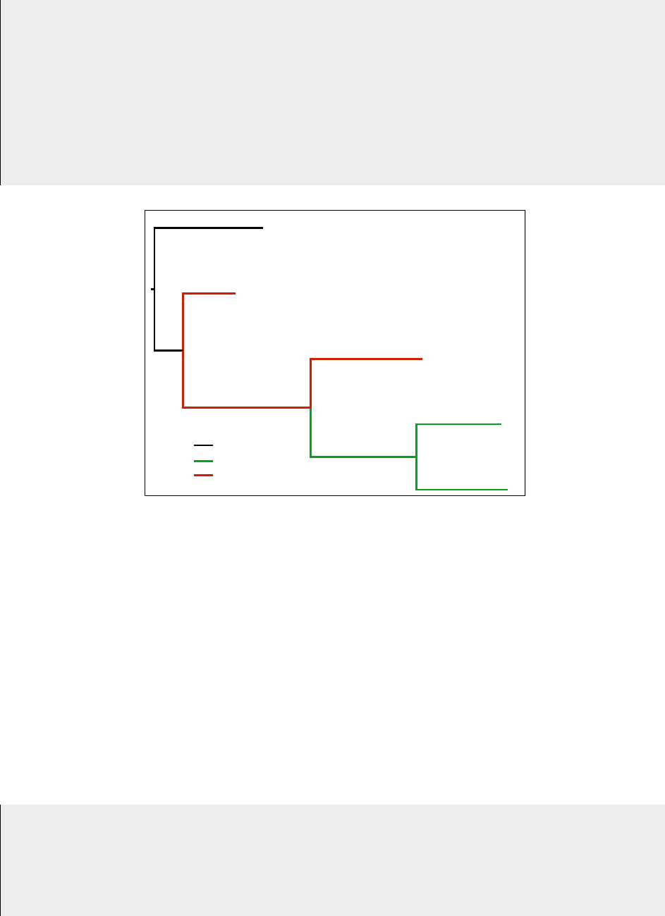
For example, a tree specified as
(t4:0.785,(t3:0.380,(t2:0.806,(t5:0.612,t1:0.660):0.762_m1_):0.921_m2_):0.207);
will be interpreted as in Figure 1. Trees with model flags, just like any other tree, are defined with the func-
tion read_tree. Some examples of trees with model flags:
1# Define a tree with propagating model flags m1 and m2, with a string
2het_tree = pyvolve.read_tree(tree = "(t4:0.785,(t3:0.380,(t2:0.806,(t5:0.612,t1:0.660)
:0.762_m1_):0.921_m2_):0.207);")
3#OR
4het_tree = pyvolve.read_tree(tree = "(t4:0.785,(t3:0.380,(t2:0.806,(t5:0.612,t1:0.660)
:0.762\#m1\#):0.921\#m2\#):0.207);")
5
6# Print het_tree to see how model flags are applied:
7pyvolve.print_tree(het_tree)
8'''
9>>> root None None
10 >>> t4 0.785 None
11 >>> internalNode3 0.207 None
12 >>> t3 0.38 None
13 >>> internalNode2 0.921 m2
14 >>> t2 0.806 m2
15 >>> internalNode1 0.762 m1
16 >>> t5 0.612 m1
17 >>> t1 0.66 m1
18 '''
19
20 # Define a tree with non-propagating model flags m1 and m2
21 het_tree = pyvolve.read_tree(tree = "(t4:0.785,(t3:0.380,(t2:0.806,(t5:0.612,t1:0.660)
:0.762_m1):0.921_m2):0.207);")
22 #OR
23 het_tree = pyvolve.read_tree(tree = "(t4:0.785,(t3:0.380,(t2:0.806,(t5:0.612,t1:0.660)
:0.762#m1):0.921#m2):0.207);")
24
25 # Print het_tree to see how model flags are applied:
26 pyvolve.print_tree(het_tree)
27 '''
23
28 >>> root None None
29 >>> t4 0.785 None
30 >>> internalNode3 0.207 None
31 >>> t3 0.38 None
32 >>> internalNode2 0.921 m2
33 >>> t2 0.806 None
34 >>> internalNode1 0.762 m1
35 >>> t5 0.612 None
36 >>> t1 0.66 None
37 '''
t4
t3
t2
t1
t5
0.785
0.762
0.66
0.806
0.38
0.207
0.612
0.921
Root model
m2 model
m1 model
Figure 1: The newick tree with model flags given by
"(t4:0.785,(t3:0.380,(t2:0.806,(t5:0.612,t1:0.660):0.762_m1_):0.921_m2_):0.207);" indicates the model assign-
ments shown.
All model flags specified in the newick phylogeny must have corresponding models. To link a model to
a model flag, specify a given model’s name using the keyword argument name when initializing a Model
object. This name must be identical to a given model flag, without the leading and trailing symbols (e.g. the
name "m1" corresponds to the flag _m1_ and/or #m1#).
The model at the root of the tree will not have a specific model flag, but nonetheless a model must be used
at the root (obviously), and indeed at all other nodes which are not assigned a model flag (not that all
branches on the tree which are not assigned a model flag will evolve according to the model used at the
root). To specify a model at the root of the tree, simply create a model, with a name, and indicate this name
when defining your partition.
Examples for defining models with names are shown below (for demonstrative purposes, nucleotide mod-
els with extreme state frequency differences are used here):
1# Define the m1 model, with frequencies skewed for AT-bias
2m1_model = pyvolve.Model("nucleotide", {"state_freqs":[0.4, 0.1, 0.1, 0.4]}, name = "
m1")
3
4# Define the m2 model, with frequencies skewed for GC-bias
5m2_model = pyvolve.Model("nucleotide", {"state_freqs":[0.1, 0.4, 0.4, 0.1]}, name = "
24

m2")
6
7# Define the root model, with default equal nucleotide frequecies
8root_model = pyvolve.Model("nucleotide", name = "root")
Alternatively, you can assign/re-assign a model’s name with the .assign_name() method:
1# (Re-)assign the name of the root model
2root_model.assign_name("new_root_model_name")
Finally, when defining the partition that uses all of these models, provide all Model objects in list to the
models argument. In addition, you must specify the name of the model you wish to use at the root of the
tree with the keyword argument root_model_name.
1# Define partition with branch heterogeneity, with 50 nucleotide positions
2temp_het_partition = pyvolve.Partition(models = [m1_model, m2_model, root_model], size
= 50, root_model_name = root_model.name)
12 Implementing branch-site heterogeneity
Simulating according to so-called "branch-site" models, in which there are both site-wise and branch het-
erogeneity, is accomplished using the same strategies shown for each individual aspect (branch, Section 11
and site, Section 10). However, there is a critical caveat to these models: all models within a given partition
must have the same number of rate categories. Furthermore, the rate probabilities must be the same across
models within a partition; if different values for rate_probs are indicated, then the probabilities provided
for the root model will be applied to all subsequent branch models. (Note that this behavior is identical for
other simulation platforms, like Indelible [3].)
The example below shows how to specify a branch-site heterogeneous nucleotide model with two models,
root and model1 (note that this code assumes that the provided phylogeny contained the flag _model1_),
when the rate categories are not equiprobable.
1# Shared rate probabilities. Must be explicitly specified for all models (not just the
root model)!
2shared_rate_probs = [0.25, 0.3, 0.45]
3
4# Construct a nucleotide model with 3 rate categories
5root = Model("nucleotide", name = "root", rate_probs = shared_rate_probs, rate_factors
= [1.5, 1.0, 0.05])
6
7# Construct a second nucleotide model with 3 rate categories
8model1 = Model("nucleotide", name = "model1", rate_probs = shared_rate_probs,
rate_factors = [0.06, 2.5, 0.11])
9
10 # Construct a partition with these models, defining the root model nameas "root"
11 part = Partition(models = [root, model1], root_model_name = "root", size = 50)
25
References
[1] M Arenas. Simulation of molecular data under diverse evolutionary scenarios. PLoS Comp Biol,
8:e1002495, 2012.
[2] MO Dayhoff, RM Schwartz, and BC Orcutt. A model of evolutionary change in proteins. Atlas of
Protein Sequence and Structure, 5(3):345–352, 1978.
[3] W Fletcher and Z Yang. INDELible: A flexible simulator of biological sequence evolution. Mol Biol
Evol, 26(8):1879–1888, 2009.
[4] N Goldman and Z Yang. A codon-based model of nucleotide substitution for protein-coding DNA
sequences. Mol Biol Evol, 11:725–736, 1994.
[5] AL Halpern and WJ Bruno. Evolutionary distances for protein-coding sequences: modeling site-
specific residue frequencies. Mol Biol Evol, 15:910–917, 1998.
[6] M Hasegawa, H Kishino, and T Yano. Dating of human-ape splitting by a molecular clock of mito-
chondrial DNA. J Mol Evol, 22(2):160–174, 1985.
[7] DT Jones, WR Taylor, and JM Thornton. The rapid generation of mutation data matrices from protein
sequences. CABIOS, 8:275–282, 1992.
[8] TH Jukes and CR Cantor. Evolution of protein molecules. In HN Munro, editor, Mammalian protein
metabolism. Academic Press, New York, 1969.
[9] C. Kosiol, I. Holmes, and N. Goldman. An empirical codon model for protein sequence evolution. Mol
Biol Evol, 24:1464 – 1479, 2007.
[10] SQ Le and O Gascuel. An improved general amino acid replacement matrix. Mol Biol Evol, 25:1307–
1320, 2008.
[11] Alexander Mirsky, Linda Kazandjian, and Maria Anisimova. Antibody-specific model of amino acid
substitution for immunological inferences from alignments of antibody sequences. Mol Biol Evol, 32:806
– 819, 2015.
[12] SV Muse and BS Gaut. A likelihood approach for comparing synonymous and nonsynonymous nu-
cleotide substitution rates, with application to the chloroplast genome. Mol Biol Evol, 11:715–724, 1994.
[13] SJ Spielman and CO Wilke. The relationship between dn/ds and scaled selection coefficients. Mol Biol
Evol, 32:1097 – 1108, 2015.
[14] S Tavare. Lines of descent and genealogical processes, and their applications in population genetics
models. Theor Popul Biol, 26:119–164, 1984.
[15] S Whelan, P de Bakker, E Quevillion, N Rodriguez, and N Goldman. PANDIT: an evolution-centric
database of protein and associated nucleotide domains with inferred trees. Nucleic Acids Res, 34:D327
– D331, 2006.
[16] S Whelan and N Goldman. A general empirical model of protein evolution derived from multiple
protein families using a maximum likelihood approach. Mol Biol Evol, 18:691–699, 2001.
[17] N Yang, R Nielsen, and M Hasegawa. MOLPHY version 2.3: programs for molecular phylogenetics
based on maximum likelihood. Comput Sci Monogr, 28:1–150, 19896.
[18] N Yang, R Nielsen, and M Hasegawa. Models of amino acid substitution and applications to mito-
chondrial protein evolution. Mol Biol Evol, 15:1600–1611, 1998.
[19] Z. Yang. Computational Molecular Evolution. Oxford University Press, 2006.
26
