Random Forests R Guide Forest In
User Manual:
Open the PDF directly: View PDF ![]() .
.
Page Count: 8

Random forests for categorical dependent variables: an informal quick start R guide
1
Random Forests for Classification Trees and Categorical Dependent Variables:
an informal Quick Start R Guide
prepared by Stephanie Shih
Stanford University | University of California, Berkeley
(last updated) 2 February 2011
Note: random forests work for continuous variables via regression trees, but I have yet to try
them for such. Thus, this quick start guide is currently limited to classification trees only.
1. Introduction
¾ What are random forests?
Random forests are a type of recursive partitioning method particularly well-suited to small n
large p problems (Strobl et al. 2009b: 339). They involve an ensemble (aka: set) of classification
(or regression) trees that are calculated on random subsets of the data, using a subset of randomly
restricted and selected predictors for each split in each classification tree (Strobl et al. 2008: §2;
Strobl et al. 2009b; a.o.). In this way, random forests are able to better examine the contribution
and behavior that each predictor has, even when one predictor’s effect would usually be over-
shadowed by more significant competitors in simpler models (e.g., simple or mixed effect
regression models) (Strobl et al. 2009b: 337). Furthermore, the results of an ensemble of
classification/regression trees have been shown to produce better predictions than the results of
one classification tree on its own (Strobl et al. 2008: §2).
Using the random forests, we also have the conditional permutation accuracy variable
importance measure available to us. Conditional variable importance is calculated by randomly
shuffling the values of a given independent variable thereby “breaking” the variable’s bond to
the response. Then, the difference of the model accuracy before and after the random
permutations, averaged over all trees in the forest, tells us how important that predictor is for
determining the outcome (Strobl et al. 2009b: 335).
¾ Why the party package?
The party package utilizes conditional inference trees, which ameliorate the bias that random
forests otherwise have towards highly correlated variables (see Strobl et al. 2008; 2009a for
further discussion).
¾ About this quick start guide
This document is meant only as a helpful listing of some R code and random forest guidelines to
get you started with the party package and random forest analyses. It is highly recommended
that you also read the references listed below in addition to the party package R
documentation, all of which have much more detail on the use and interpretation of random

Random forests for categorical dependent variables: an informal quick start R guide
2
forest statistics than is included here. This document is also by no means a complete listing of R
code for random forest statistics, and it will be continually updated with more code and methods.
All lines of actual R code are listed with a “>” preceding them for readability. Do not copy this
arrow when using the code in R.
2. A Very Important Note about Random Forests
Random forests are a truly ‘random’ statistical method in that the model results can vary from
run to run. Therefore, it is of utmost importance that you verify the stability of your forests by
starting with at least one different seed (see §5) and by increasing the size of your forest (§4) to
a sufficiently large number (Strobl 2009a: 17; Strobl 2009b: 343 for a more extensive
discussion). Variable importance (§6), as well, should be interpreted and reported as a relative
ranking of significant predictors, and “the absolute values of the importance scores should not be
interpreted or compared over different studies” (Strobl 2009b: 336).
3. Installing and loading R libraries
To download the party package, go to (on the top toolbar in the R console) Packages > Install
packages > (select a CRAN mirror nearest to you) > (select packages to download).
For the code included in this document, you’ll need at least the Hmisc, lattice, and party
libraries. I’d recommend installing languageR, Design, and party instead just to cover all
of your bases.
Load the libraries in the R console using the following code.
> library(languageR)
> library(Design)
> library(Party)
For convenience, you can also write this code into your .Rprofile file so that R automatically
loads the packages whenever you start the program.
4. Model parameters
¾ Don’t forget to report the model parameters used when reporting results of random forest
analyses!
Set controls for the random forest.
> data.controls <- cforest_unbiased(ntree=1000, mtry=3)
Random forests for categorical dependent variables: an informal quick start R guide
3
Notes on model parameters:
ntree (default = 500)
= overall number of trees in the forest
The number of trees should be increased as the number of variables or data points increase. A
suitably large number of trees will guarantee more stable and robust results. (e.g., having
ntree=8000 for a sparse dataset with a large number of predictors is not unheard of.)
mtry (default = 5)
= number of randomly preselected predictor variables for each split
Square root of the number of variables (suggested; see Strobl et al. 2009c: 3)
5. Running the random forest
Set a random seed for your forest run. Any random number will do!
> set.seed(47)
Running a random forest:
> data.cforest <- cforest(Resp ~ x + y + z…, data = mydata,
controls=data.controls)
where “Resp” = dependent variable*;
x, y, z = independent variable;
mydata = name of your dataframe;
data.controls = model parameters set using cforest_unbiased()
*IMPORTANT: When using categorical variables, make sure they are encoded as factors, not as
numeric. Use class(data$Resp) to check the encoding, and use
as.factor(data$Resp) to encode your vector as a factor.)
6. Permutation Accuracy Variable Importance
> data.cforest.varimp <- varimp(data.cforest, conditional =
TRUE)
(Note: conditional variable importance will take a while and is fairly CPU-intensive, especially
for data sets with many variables, observations, and levels to the variables. I would highly
recommend running these calculations on a high-powered computer.)
Random forests for categorical dependent variables: an informal quick start R guide
4
A sample read-out of the conditional variable importance results:
> data.cforest.varimp
A B C D E
0.0099337753 0.0016181685 0.0002009447 0.0034510738 -0.0005742108
F G H I
0.0036466314 0.0072089218 -0.0014413413 0.0010496797
¾ How to interpret variable importance results
Variables can be considered informative and important if their variable importance value is
above the absolute value of the lowest negative-scoring variable. “The rationale for this rule of
thumb is that the importance of irrelevant variables varies randomly around zero” (Strobl et al.
2009b: 342). As mentioned in §2, results from random forests and conditional variable
importance should always be verified via multiple random forest runs starting with different
seeds and sufficiently large ntree values to insure the robustness and stability of results (Strobl
et al. 2009b: 343).
To export your variable importance results as a table for later data visualization:
> write.table(data.cforest.varimp, file="FILEPATH.txt")
(This is especially useful if you are running your random forest variable importance calculations
on a remote server without a graphical interface.)
7. Visualizing variable importance
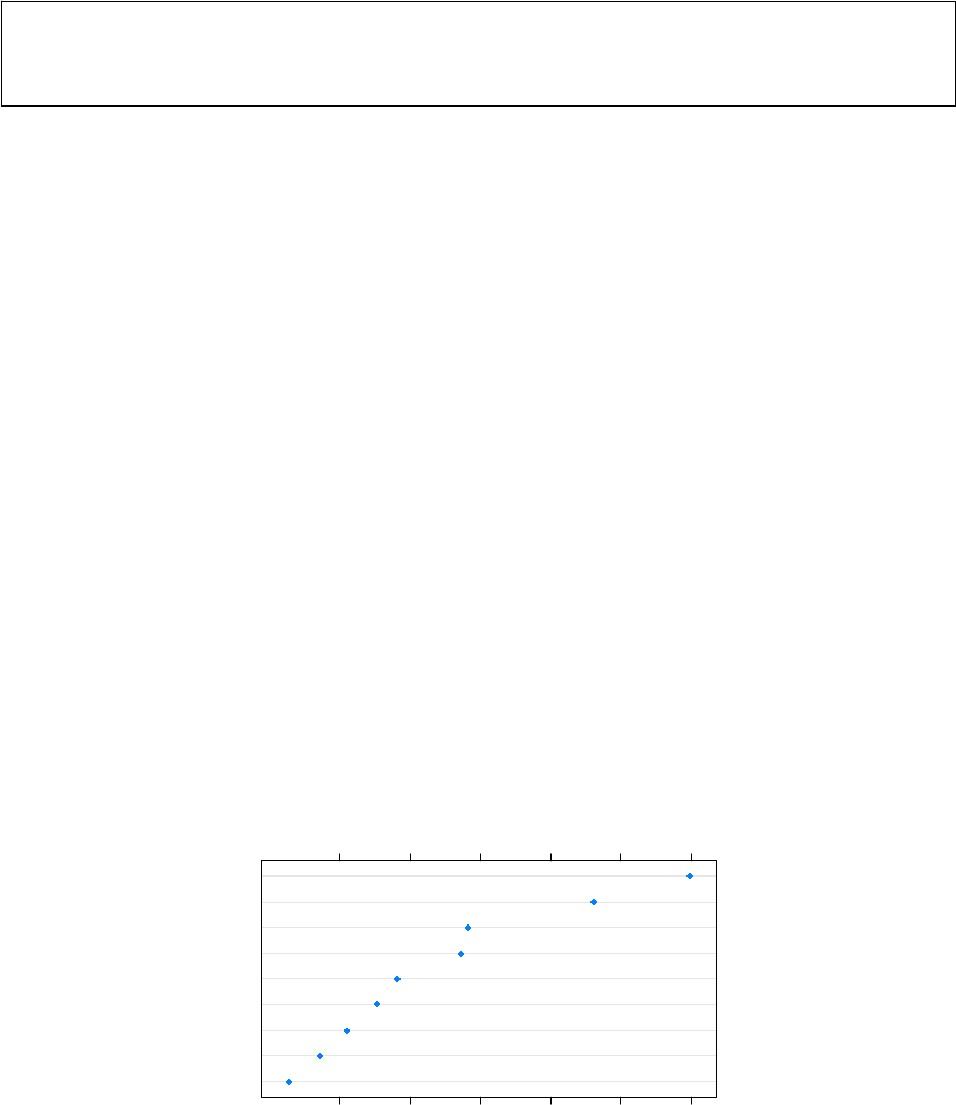
¾ Dot plots
A simple dotplot of the variable importance results
> dotplot(sort(data.cforest.varimp))
sort(data.cforest.varimp)
H
E
C
I
B
D
F
G
A
0.000 0.002 0.004 0.006 0.008 0.010
Random forests for categorical dependent variables: an informal quick start R guide
5
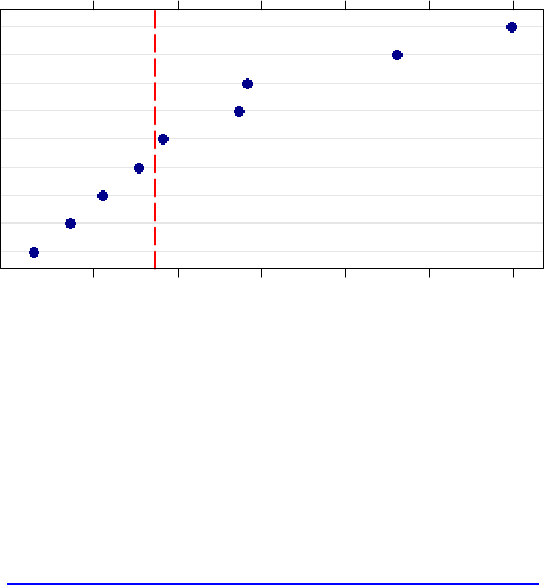
To aid the interpretation of variable importance results, you can add a line on the plot at the
absolute value of the lowest ranking predictor (see §6 for explanation).
> dotplot(sort(data.cforest.varimp), xlab=”Variable Importance
in DATA\n(predictors to right of dashed vertical line are
significant)”, panel = function(x,y){
panel.dotplot(x, y, col=’darkblue’, pch=16, cex=1.1)
panel.abline(v=abs(min(data.cforest.varimp)), col=’red’,
lty=’longdash’, lwd=2)
}
)
Notes on graphical parameters:
cex
changes the size of the dots in the dotplot. .5 = 50% of default size, 1.5 = 150% of default size.
pch
changes dot type. See http://www.statmethods.net/advgraphs/parameters.html for a list as well as
additional information on graphical parameters.
Variable Importance in mydata
(predictors to right of dashed vertical line are significant)
H
E
C
I
B
D
F
G
A
0.000 0.002 0.004 0.006 0.008 0.010
Random forests for categorical dependent variables: an informal quick start R guide
6
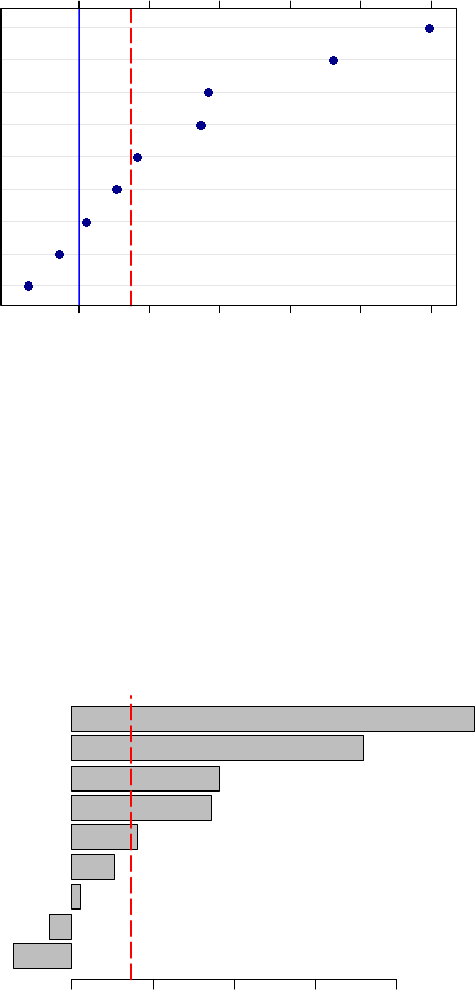
You can also insert a blue line at 0 on the x-axis. Before the closing “}” in the code above, insert
this following line.
panel.abline(v=0, col=’blue’)
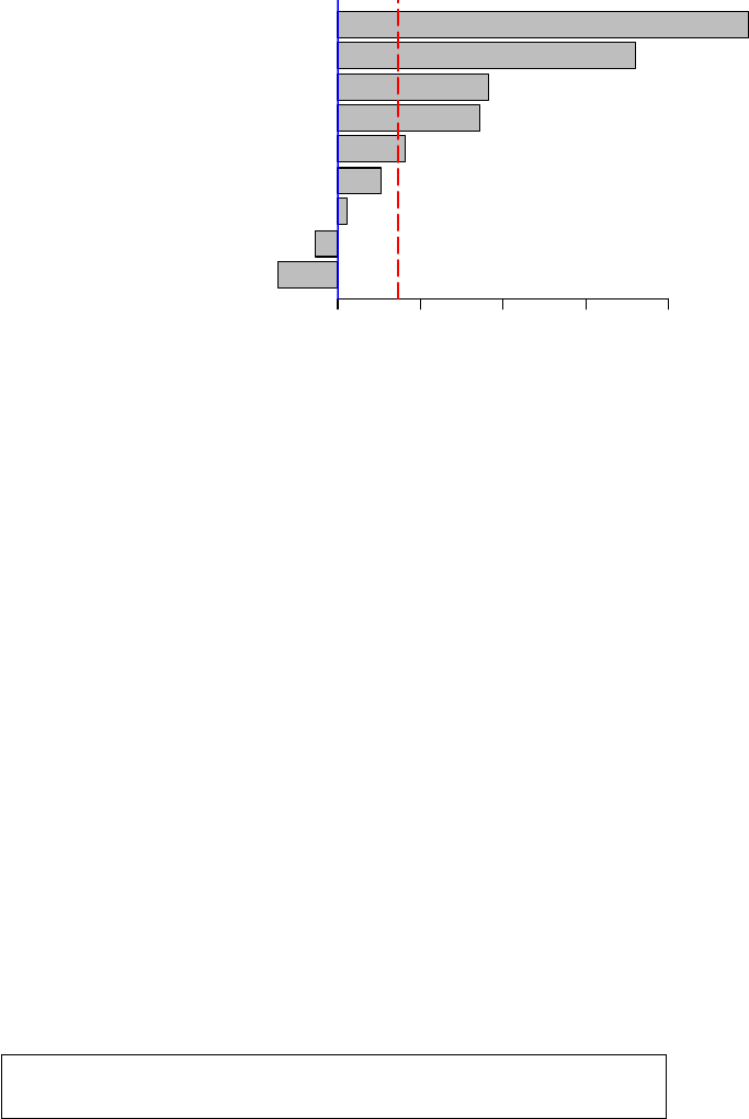
¾ Barplots
> barplot(sort(data.cforest.varimp), horiz=TRUE, xlab=”Variable
Importance in mydata\n(predictors to right of dashed vertical
line are significant)")
> abline(v=abs(min(data.cforest.varimp)), col=’red’,
lty=’longdash’, lwd=2)
Variable Importance in DATA
(predictors to right of dashed vertical line are significant)
H
E
C
I
B
D
F
G
A
0.000 0.002 0.004 0.006 0.008 0.010
HEC I BDFGA
Variable Importance in mydata
(predictors to right of dashed vertical line are significant)
0.000 0.002 0.004 0.006 0.008
Random forests for categorical dependent variables: an informal quick start R guide
7
To insert a blue line at 0 on the x-axis:
> abline(v=0, col=”blue”)
¾ Saving plots
To save plots for use in Microsoft Office, use .emf filetypes.
> savePlot(filename=”FILEPATH/filename”, type=c(“emf”))
The type argument also supports .png, .jpeg, .jpg, .bmp, .ps, .eps, and .pdf file types.
You’ll want .ps or .eps files for LaTeX use:
> savePlot(filename=”FILEPATH/filename”, type=c(“eps”))
8. Model statistics and predictions
Obtaining the C statistic and Somers’ Dxy
> data.trp <- treeresponse(data.cforest)
> data.predforest <- sapply(data.trp, FUN = function(v)
return(v[1]))
> somers2(data.predforest, mydata$Resp)
C Dxy n Missing
0.8447197 0.6894393 410.0000000 0.0000000
HEC I BDFGA
Variable Importance in mydata
(predictors to right of dashed vertical line are significant)
0.000 0.002 0.004 0.006 0.008

Random forests for categorical dependent variables: an informal quick start R guide
8
---
Select References
Hothron, Torsten; Kurt Hornik; and Achim Zeileis. 2006. Unbiased recursive partitioning: A conditional
framework. Journal of Computational and Graphical Statistics. 15(3): 651-674.
Hothorn, Torsten; Kurt Hornik; Carolin Strobl; and Achim Zeileis. 2010. A Laboratory for Recursive
Partytioning. < http://cran.r-project.org/web/packages/party/party.pdf>
Strobl, Carolin; Anne-Laure Boulesteix; Thomas Kneib; Thomas Augustin; and Achim Zeileis. 2008.
Conditional variable importance for random forests. BMC Bioinformatics. 9: 307.
Strobl, Carolin; Torsten Hothorn; and Achim Zeileis. 2009a. Party on! A new, conditional variable-
importance measure for random forests available in party package. The R Journal. 1/2: 14-17.
Strobl, Carolin; James Malley; and Gerhard Tutz. 2009b. An Introduction to Recursive Partitioning:
Rational, Application, and Characteristics of Classification and Regression Trees, Bagging, and
Random Forests. Psychological Methods. 14(4): 323-348.
Strobl, Carolin; James Malley; and Gerhard Tutz. 2009c. Supplement to ‘An Introduction to Recursive
Partitioning: Rational, Application, and Characteristics of Classification and Regression Trees,
Bagging, and Random Forests. <http://dx.doi.org/10.1037/a0016973.supp> accessed 11
November 2010.
---
Acknowledgements to Joan Bresnan for much R and statistics aid, code, and feedback.
---
Questions? Comments? Mistakes? Suggestions?
Contact: Stephanie Shih
mailto:stephsus@stanford.edu
Quick guide download: http://www.stanford.edu/~stephsus/R-randomforest-guide.pdf
