Rss Ringoccs User Guide
User Manual:
Open the PDF directly: View PDF ![]() .
.
Page Count: 31
- Introduction
- Setting Things Up
- Using rss_ringoccs
- A detailed look at the rss_ringoccs software package
- Where To Go From Here
- Acknowledgements
- Meta Kernel File
- Frequency Offset Fitting GUI
- Free Space Power Fitting
- Acronyms
- Glossary

rss ringoccs: User Guide
Richard G. French∗
,Sophia R. Flury, Jolene W. Fong,
Ryan J. Maquire, and Glenn J. Steranka
∗Cassini Radio Science Team Leader
September 30, 2018

Contents
1 Introduction 1
1.1 Getting help ............................................ 1
1.2 What is an RSS ring occultation? ................................ 1
1.3 Overview of Cassini RSS ring observations ........................... 1
1.4 Cassini RSS ring occultation observations on NASA’s PDS ................. 2
1.4.1 Raw RSS data files .................................... 3
1.4.2 Higher-level products .................................. 3
1.5 Required and recommended reading .............................. 4
1.5.1 Cassini Radio Science User’s Guide ........................... 4
1.5.2 Marouf, Tyler, and Rosen (1986) - MTR86 ...................... 4
1.5.3 For more information... ................................. 4
2 Setting Things Up 4
2.1 System requirements ....................................... 4
2.2 Install Python 3 and required packages ............................. 5
2.2.1 Download and install spiceypy ............................. 5
2.2.2 Test spiceypy ...................................... 5
2.3 Download and install the rss ringoccs repository from GitHub .............. 5
2.4 Download the required JPL/NAIF SPICE kernels ....................... 6
2.5 Download essential Cassini RSS raw data files ........................ 8
3 Using rss ringoccs 8
3.1 Python Object Orientated Programming ............................ 8
3.2 Conventions and Hierarchy ................................... 9
3.3 Testing rss ringoccs: the Huygens Ringlet ......................... 9
3.4 End-to-end Pipeline: A Second Look at the Huygen’s Ringlet ................ 10
3.5 Quick-Look Method: Comparing Profiles Reconstructed at Different Resolutions ..... 12
4 A detailed look at the rss ringoccs software package 13
4.1 Pipeline Outline ......................................... 13
4.2 RSR Reader ............................................ 13
4.3 Occultation geometry routines ................................. 14
4.4 Calibration routines ....................................... 14
4.5 Diffraction-limited Profile Routines ............................... 16
4.6 Diffraction reconstruction routines ............................... 16
4.7 Utility routines .......................................... 19
5 Where To Go From Here 20
5.1 The Cassini RSS data catalog .................................. 20
5.2 Selecting an RSR file to process ................................. 21
5.3 Benchmarks ............................................ 21
5.4 Licensing ............................................. 21
Acknowledgements 22
A Meta Kernel File 23
B Frequency Offset Fitting GUI 23
C Free Space Power Fitting 24
Acronyms 26
Glossary 27
i
List of Figures
1 Ring opening angle vs. year ................................... 2
2 Earth view of Cassini during the Rev007 and Rev054 ring occultation observations. . . . 2
3 Huygens ringlet initial test figure ................................ 10
4 Rev007E Maxwell Ringlet at different resolutions ....................... 12
5 Data processing pipeline ..................................... 13
6 Frequncy Offset GUI ....................................... 24
7 Free Space Power GUI ...................................... 25
List of Tables
1 Hardware and Operating Systems ................................ 4
2 Python Versions ......................................... 5
3 Glossary of parameters in the *GEO.TAB file ......................... 14
4 Glossary of Data from the Cal File ............................... 15
5 Glossary of Parameters in Tau File ............................... 16
6 Glossary of Parameters in Tau File ............................... 16
7 Benchmarks for the rev7E X43 16kHz file ........................... 21
ii

1 Introduction
The Cassini Radio Science Subsystem (RSS) was used during the Cassini orbital tour of Saturn to observe
a superb series of ring occultations that resulted in high-resolution, high-SNR radial profiles of Saturn’s
rings at three radio wavelengths: 13 cm (S band), 3.6 cm (X band), and 0.9 cm (Ka band). Radial optical
depth profiles of the rings at 1- and 10-km resolution produced by the Cassini RSS team, using state-of-
the-art signal processing techniques to remove diffraction effects, are available on the NASA Planetary
Data System (PDS).1These archived products are likely to be quite adequate for many ring scientists,
but for those who wish to generate their own diffraction-reconstructed ring profiles from Cassini RSS
observations, we offer rss ringoccs: a suite of Python-based analysis tools for radio occultations of
planetary rings.2
The purpose of rss ringoccs is to enable scientists to produce “on demand” radial optical depth profiles
of Saturn’s rings from the raw RSS data, without requiring deep familiarity with the complex process-
ing steps involved in calibrating the data and accounting for the effects of diffraction. The code and
algorithms are extensively documented, providing a starting point for users who wish to test, refine, or
optimize the straightforward methods we have employed. Our emphasis has been on clarity, sometimes
at the expense of programming efficiency and execution time. rss ringoccs does an excellent job of
reproducing existing RSS processed ring occultation data already present on NASA’s PDS Ring-Moon
Systems Node, but we make no claim to having achieved the state-of-the-art in every respect. We en-
courage users to augment our algorithms and to report on those improvements, so that they can be
incorporated in future editions of rss ringoccs.
This document provides an introduction to RSS ring occultations, directs users to required and recom-
mended reading, describes in detail how to set up rss ringoccs, and explains how to obtain RSS data
files and auxiliary files required by the software. It provides an overview of the processing pipeline, from
raw data to final high-resolution radial profiles of the rings, and guides users through a series of simple
examples to illustrate the use of rss ringoccs.
1.1 Getting help
rss ringoccs is easy to install and use, but if you have questions along the way, please don’t hesitate
to get in touch with us. We recommend that you post an issue to the rss ringoccs repository3so that
other users can join in the conversation, but you are also free to contact the lead author of the project
at the email address on the title page of this document.
1.2 What is an RSS ring occultation?
Simply put, an RSS ring occultation occurs when a radio signal transmitted from a spacecraft’s High
Gain Antenna (HGA) passes through the rings on the way to a Deep Space Network (DSN) receiving
antenna on Earth. The received signal at Earth is affected by interactions of the radio signal with the
swarm of ring particles, including attenuation, scattering, Doppler-shifting of the signal, and diffraction.
We refer to the process of compensating for diffraction to obtain the intrinsic radial optical depth profile
of the rings as diffraction reconstruction or Fresnel inversion, since the reconstruction process is based
on the mathematical principles of Fresnel optics.
1.3 Overview of Cassini RSS ring observations
Over the course of the Cassini orbital tour of Saturn, the geometry of RSS ring occultations varied due
both to changes in the orbiter’s trajectory and to the aspect of the rings as seen from Earth during
Saturn’s orbit around the Sun. The opening angle of Saturn’s rings as a function of time as seen from
Earth is shown below in Fig. 1.
1https://pds-rings.seti.org/cassini/rss/index.html
2rss ringoccs may be obtained from https://github.com/NASA-Planetary-Science/rss_ringoccs
3https://github.com/NASA-Planetary-Science/rss_ringoccs/issues
1
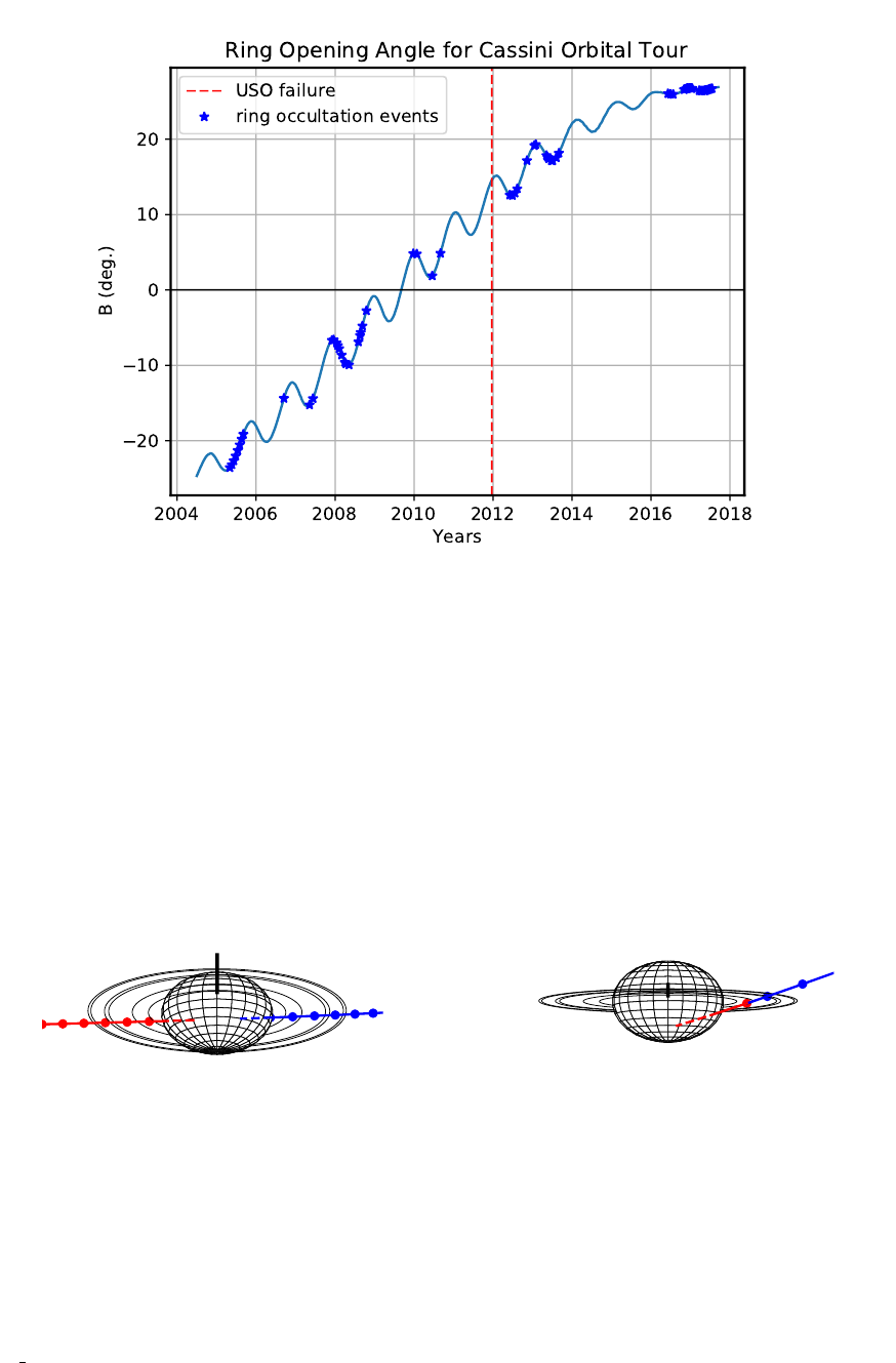
Fig. 1: Ring Opening angle (B) vs. Time. Dark line indicates an opening angle of B= 0 where the ring system is edge-on. In
2012, the ultra-stable oscillator (USO) failed, complicating diffraction reconstruction thereafter.
Individual occultations are identified by the Cassini rev number n, corresponding roughly to the nth
passage of Cassini around Saturn during which the occultation occurred. During the ingress portion of
an occultation, the orbital radius of the intercept point in the ring plane of the incident ray from the
spacecraft decreases with time; the radius increases with time during the egress portion of an occulta-
tion. During a diametric occultation, the ingress and egress portions of the occultation are interrupted
by passage of the spacecraft behind the planet itself as seen from Earth, resulting in an atmospheric
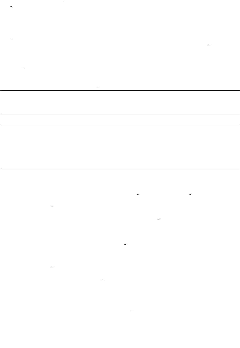
occultation. The view from Earth of the ingress and egress portions of a diametric occultation on Rev
7 is shown in Fig. 1.2.1 below, in blue and red lines, respectively, with the atmospheric occultation
portions in dashed lines. During a chord occultation, the ingress and egress occultations are contiguous.
The view from Earth of the chord occultation on Rev 54 is shown in Fig. 1.2.2 below.
1.2.1: Rev007 1.2.2: Rev054
Fig. 2: Earth view of Cassini during the Rev007 and Rev054 ring occultation observations.
1.4 Cassini RSS ring occultation observations on NASA’s PDS
There are two categories of Cassini RSS observations on the PDS: raw data in Radio Science Receiver
(RSR) files that contain the digitized spacecraft signal as received at the DSN, and higher-level products
(reduced data) that have been processed by the RSS team, including diffraction-reconstructed radial
profiles of the optical depth of Saturn’s rings and associated geometric and calibration information.
rss ringoccs processes raw RSR files and independently produces higher-level products that can be
saved as files similar in form and content to those already on the PDS, but with a user-defined radial
resolution.
2

1.4.1 Raw RSS data files
The raw data produced by the DSN that contain the original observations of all Cassini occultation
observations are recorded in RSR files, described in more detail in the Cassini Radio Science Users Guide
(Section 1.5.1). During Cassini RSS occultations, RSR files were typically recorded at two bandwidths:
1 kHz and 16 kHz. The rss ringoccs package can handle either version, and they give nearly identical
results, although the processing time for the 16 kHz files is slightly longer.
At the present time, only the 16 kHz files are available on the PDS, although there are plans to archive
the 1 kHz files (likely during 2019). We provide convenient scripts in rss ringoccs (Section 2.5) to
download 16 kHz RSR files from the PDS archive.
1.4.2 Higher-level products
Essam Marouf of the Cassini RSS team has produced two sets of higher-level products for ring occultation
observations. The first can be found at https://pds-rings.seti.org/cassini/rss/index.html. This
archive set contains 1- and 10-km resolution diffraction-reconstructed profiles from X-band observations
of Revs 7 through 67. First, navigate to the dataset CORS 8001 and then to the EASYDATA subdirectory.
Within this directory, occultation data sets are organized by name: RevXXev RSS YYYY DOY B## D/ (e.g.,
Rev07E RSS 2005 123 X43 E/) where:
•XX is the rev number (ex: 07)
•ev is the event type (ex: E)
Ifor ingress
Efor egress
CI for ingress portion of chord occultation
CE for egress portion of chord occultation
•YYYY is the UTC year of the start of the occultation (ex: 2005)
•DOY is the UTC day of year of the start of the occultation (ex: 123)
•Bindicates the frequency band in which the observations were made (ex: X)
•## indicates the numeric code for the DSN station from which the observations were made (ex: 43)
•Dis the direction (Ifor ingress, Efor egress) (ex: E)
Each occultation data set directory contains a set of *.LBL label files that describe counterpart *.TAB
ASCII data tables or a summary PDF file. For example:
•Rev07E RSS 2005 123 X43 E Summary.pdf contains an overview of the occultation
•RSS 2005 123 X43 E CAL.LBL,TAB contain calibration information
•RSS 2005 123 X43 E GEO.LBL,TAB contain geometry information
•RSS 2005 123 X43 E TAU 01KM.LBL,TAB contain the diffraction-reconstructed optical depth profile
of the rings at 1 km processing resolution.
•RSS 2005 123 X43 E TAU 10KM.LBL,TAB contain the diffraction-reconstructed optical depth profile
of the rings at 10 km processing resolution.
A second set of higher-level products, the Casssini RSS Ring Profiles 2018 Archive, produced by RSS
team member Essam Marouf, has just completed peer review by the PDS. It contains reconstructed
optical depth profiles at 1- and 10-km processing resolution for all S, X, and Ka-band ring occultation
observations from Revs 7 through 137. In addition to the file types enumerated above, this second set of
archive produces includes intermediate diffraction-limited profile (DLP) files that contain the normalized
diffraction-limited observations that are the input for the diffraction reconstruction stage of the analysis
4. Once this second delivery of higher-level products has been officially accepted by the PDS in its final
form, this document will be updated to provide additional details about these higher-level products.
4We have used these results to provide independent tests of the ability of rss ringoccs to process the raw data up to
the point of diffraction-limited profiles, and to perform the diffraction reconstruction to produce final optical depth profiles.
3

rss ringoccs has the ability to produce CAL, GEO, DLP, and TAU label and table files that users can
compare directly with the two sets of higher-order products just described. For comparability and consis-
tency, the .LBL and .TAB files are in PDS3 format following the Casssini RSS Ring Profiles 2018 Archive
submitted by Essam Marouf.
1.5 Required and recommended reading
With this overview of RSS ring occultation observations and data in hand, we strongly recommend that
all users familiarize themselves with several key documents before use of the rss ringoccs package.
Our internal documentation of the rss ringoccs code makes frequent reference to the following two
documents:
1.5.1 Cassini Radio Science User’s Guide
The most complete practical introduction to Cassini RSS ring observations is contained in the Cassini
Radio Science User’s Guide5. We regard this as required reading. Chapter 2 describes the open-loop RSR
files that contain the raw RSS ring occultation data, and Chapter 3.3 summarizes the analysis steps to
produce a diffraction reconstruction ring optical depth profile from the observations. For the remainder
of this guide, we will assume that all readers have familiarized themselves with this material.
1.5.2 Marouf, Tyler, and Rosen (1986) - MTR86
The definitive reference for diffraction reconstruction of RSS occultations is Marouf et al. 1986: Marouf,
Tyler and Rosen’s classic “Profiling Saturn’s rings by radio occultation” – we refer to this as MTR86. For
copyright reasons, we cannot include MTR86 in this GitHub repository, but we highly recommend that
scientists making use of radio occultation data have this paper readily at hand. It documents the Fresnel
inversion method of diffraction reconstruction, complete with application to Voyager RSS occultation
observations of Saturn’s rings. This is recommended reading for beginning users of rss ringoccs, and
required reading for anyone wishing to understand the inner workings of the rss ringoccs software
package.
1.5.3 For more information...
Readers interested in an overview of Cassini RSS instrumentation and science goals are encouraged to
read Kliore et al.’s “Cassini Radio Science” (Kliore et al. 2004). Scientific results making use of Cassini
RSS occultation observations include Colwell et al. 2009,Moutamid et al. 2016,French et al. 2016a,
French et al. 2016b,French et al. 2017 and Marouf et al. 2011,Nicholson et al. 2014a,Nicholson et al.
2014b,Rappaport et al. 2009,Thomson et al. 2007.
2 Setting Things Up
This section provides step-by-step instructions on setting up the rss ringoccs package and associated
data files. We assume that all users are familiar with basic unix commands and introductory-level
Python.
2.1 System requirements
The rss ringoccs repository has been developed and tested on the following hardware, unix-based
operating systems, and shells:
Hardware Operating System Shell GB of RAM
MacBookPro, iMac MacOS High Sierra 10.13.4 csh, bash 8, 16, and 32
Mac mini Linux Ubuntu Budgie 16 bash 8
MacBookPro Linux Ubuntu 16 bash 8
ThinkMate Linux Debian bash 32
Table 1: Hardware and Operating Systems
5Available from https://pds-rings.seti.org/cassini/rss/
4

We strongly recommend that users run rss ringoccs on a system with at least 16 GB of RAM (preferably
32 GB), to minimize disk-based memory swapping, which can significantly increase the run time when
processing an entire occultation at high resolution.
2.2 Install Python 3 and required packages
rss ringoccs has been tested with Python 3, in particular Python 3.5 and 3.6. Our code has been
tested under the following Python configurations:
Operating System Python Distribution Version URL
MacOS 10.13.4 Enthought Canopy Python 3.5.2 https://www.enthought.com
MacOS 10.13.4 Anaconda Python 3.6.3 https://www.anaconda.com
Linux Ubuntu Budgie 16 Anaconda Python 3.6.3 https://www.ubuntu.com
Linux Ubuntu 16 Anaconda Python 3.6.3 https://www.ubuntu.com
Linux Debian Anaconda Python 3.6.3 https://www.debian.org
Table 2: Python Versions
Install the following Python packages required by rss ringoccs, illustrated here using pip.6Enter the
following commands in a terminal at the unix command line:
host:∼user$ pip install ma tplot lib
host:∼user$ pip install numpy
host:∼user$ pip install p ytest
host:∼user$ pip instal l six
host:∼user$ pip install scipy
2.2.1 Download and install spiceypy
rss ringoccs makes extensive use of JPL’s NAIF SPICE toolkit Acton 1996, a set of software tools to
calculate planetary and spacecraft positions, ring occultation geometry, and a host of useful calendar
functions.7Our software requires spiceypy, a Python-based interface to the NAIF toolkit, available from
https://github.com/AndrewAnnex/SpiceyPy. Follow the installation instructions on this website, or
use pip:
host:∼user$ pip install spic ey py
2.2.2 Test spiceypy
To test your installation of spiceypy, fire up Python in a terminal at the unix command line and at
the >>> prompts, enter the following commands, and confirm that spiceypy returns πand the speed of
light c:
host:∼user$ pyt hon
>>> from __fut ure__ import pri nt_ fun cti on
>>> import s pi ceypy
>>> print ( spi ce ypy . pi () , sp ic eypy . clight ())
3. 1415 926 535 897 93 29 9792. 458
>>> exit ()
2.3 Download and install the rss ringoccs repository from GitHub
Follow these steps to download and install rss ringoccs:
•Visit https://github.com/NASA-Planetary-Science/rss_ringoccs and click the green Clone
or Download pull-down menu at the upper right.
6https://pip.pypa.io/en/stable/
7See https://naif.jpl.nasa.gov/naif/index.html
5

•Download the zip file rss ringoccs-master.zip to your local Downloads directory. For this
example, this is ∼/Downloads.
•Identify the destination directory under which you wish to install rss ringoccs. For this example,
the destination directory is ∼/local. (This should be on a large-capacity disk drive or partition
– 1 TB or larger – since raw Cassini RSS data files are quite large. We recommend that this be
routinely backed up.)
•Use your favorite utility to unzip the file. This will create the rss ringoccs-master directory and
several sub-directories. For example:
host:∼user$ cd ∼/ local
host:∼user$ unzip ∼/ Down loads / rss_r in go ccs - master . zip
host:∼us er$ ls -1 F rss *
rss_ringoccs -master:
AA REA DM E . txt
LICENSE
data/
docs/
examples/
kernels/
output/
pipeline/
rss_ringoccs/
tables/
README.md
•The current software release of rss ringoccs follows the naming conventions and hierarchy used
on the PDS with some minor changes. Below, we provide a brief description of the top-level
directories for reference.
|-data/............... RSR and other raw science data files
|-docs/............... Documentation
|-examples/........... Example scripts covered in the User’s Guide
|-kernels/............ Kernel files from NASA/NAIF/SPICE
|-output/............. *.LBL, *.TAB, pickle, and plot files produced by the software
|-pipeline/........... Pipeline scripts for end-to-end and quick-look execution
of the software
|-rss_ringoccs/....... Source code
|-tables/............. Reference files tabulating kernel and RSR files available
from NAIF and the PDS
For a detailed description of the organization of the package, see the AAREADME.MD file contained
in the top-level directory of the software release: rss ringoccs-master. The so-called “pickle”
output file is a binary storage of a Python dictionary output and input by the Python package
pickle8.
2.4 Download the required JPL/NAIF SPICE kernels
The rss ringoccs package makes extensive use of SPICE data (kernel files) from JPL/NAIF that
specify planetary and spacecraft ephemerides, planetary constants, and other essential information for
computing the geometric circumstances of occultations.9rss ringoccs contains bash-based shell scripts
to automate the retrieval of SPICE kernels from the NAIF website and store them in subdirectories under
rss ringoccs/kernels/, following the same directory structure as on the NAIF ftp site. Some of the
kernel files are quite large, and will take some time (and significant disk space) to download. For quick
setup and testing purposes, a minimal set of essential kernels is required. To download these, navigate
to the directory containing the rss ringoccs-master directory, and enter the following commands at
the command line of a terminal window:
8https://docs.python.org/3/library/pickle.html
9For detailed information about kernels, visit https://naif.jpl.nasa.gov/naif/data.html
6

host:∼user $ cd rss_ ri ng oc cs - maste r / pi peli ne
host:∼user $ ./ get _ke rn els .sh ../ exa mpl es / R ev007 _l is t_ of _k ernel s . txt ../ kernels /
host:∼user $ cd ../ ker nels
host:∼user $ ls -lR
You should have a listing that resembles the following:
AAREADME_kernels.txt
naif
./ naif :
CASSINI
generic_kernels
./ naif / C ASS INI :
kernels
./ naif / CASSINI / kernels :
lsk
pck
spk
./ naif / CASSINI / kernels / lsk :
na if0 01 2 . tls
./ naif / CASSINI / kernels / pck :
cp ck 26 Feb 20 09 . tpc
earth_000101_180919_180629.bpc
./ naif / CASSINI / kernels / spk :
05 0606 R_S CP SE _0 5114 _0 51 32 . bsp
./ naif / gene ric _ke rne ls :
spk
./ naif / gene ric _ke rne ls / spk :
planets
stations
./ naif / gene ric _ke rne ls / spk / planets :
de 43 0 . bsp
./ naif / gene ric _ke rne ls / spk / st ations :
earthstns_itrf93_050714.bsp
You will notice that there are several Cassini-specific kernel files. Among them are the so-called re-
constructed trajectory files. For example, 050606R SCPSE 05114 05132.bsp is a reconstructed Cassini
trajectory file produced on 2005 June 6 (050606) that spans the period 2005 day of year 114 to 132
(05114 to 05132), or April 24 to May 12, 2005. This reconstructed trajectory file is specific to each Rev
and should be specified in the meta kernel.
In order to compute the geometry of RSS occultations throughout the Cassini orbital tour, a larger set
of these large trajectory files is required. Once you have completed the initial tests of rss ringoccs, we
recommend that you download this more complete set of files, using the commands below:
host:∼user$ cd rss_ ringoc cs - master / pipeli ne
host:∼user$ ./ get_k ern els . sh ../ tables / lis t_o f_k ern els . txt ../ kernels /
The shell script detects whether a given kernel has already been downloaded, so you may interrupt
this command if it hasn’t run to completion in the time you have available, and repeat the com-
mand later, picking up the downloading process where it left off the previous time. (NOTE: if you
stop the get kernels.sh script while it is downloading a file, the file may be incomplete but will
still be detected by future shell scripts as having been downloaded. You will need to delete incom-
plete files to restart the download. To check for incomplete files, look in the lsk,pck, and spk
7
directories within the rss ringoccs-master/kernels/naif/CASSINI/kernels/ directory and in the
rss ringoccs-master/kernels/naif/generic/kernels/ directory. The most likely incomplete files
will be .bsp files located in the spk/ directory where kernel files for each occultation set of spacecraft
and planetary ephemerides are stored; however, it is best to check all kernel directories.) Once you have
downloaded the complete set of kernels, you will not need to repeat this process unless JPL releases an
updated set of Cassini trajectory files. We plan to update this documentation and the input files for
get kernels.sh if that occurs. The metakernel for the total set of Cassini and Saturn kernels is located
in ../tables/Sa-TC17-V001.ker, which the user will need to reference when running rss ringoccs.
2.5 Download essential Cassini RSS raw data files
The rss ringoccs package requires local access to raw Cassini RSS data files (Section 1.4.1). The
storage capacity on GitHub is not sufficient to allow even one sample RSR file to be part of the standard
download. Instead, as with the kernels files described above, we provide a script to download a minimal
set of RSR files for the initial tests of rss ringoccs:
host:∼user $ cd rss_ ri ng oc cs - maste r / pi peli ne
host:∼user $ ./ g et_ rsr_ fi les . sh ../ exa mp les / Rev0 07_ li st _of_r sr_ fi le s . txt ../ data /
host:∼user $ cd ../ data
host:∼user $ ls -lR
You should have a listing the resembles the following:
AA RE AD ME_ da ta . txt
co - s -rss -1 - sroc1 - v10 /
co rs _0105 /
sr oc 1_123 /
rsr /
s10sroe2005123_0740nnnx43rd.2a2
s10sroe2005123_0740nnnx43rd.LBL
The deeply-nested directory structure of the downloaded data follows that of the PDS website from
which the RSR files are retrieved so that users can easily determine the original source of each RSR
file. (Note that only a subset of the RSS files on the PDS is downloaded; the complete PDS distribution
contains many additional files that are not needed by rss ringoccs.) The cors xxxx prefix refers to
the Cassini Orbiter Radio Science PDS delivery xxxx. Underneath these directories are directories with
names such as sroc1 123, which somewhat cryptically refers to a Saturn ring occultation (sroc) on
day of year 123 of the year during which the data were taken. The RSR files of interest are located
in next level rsr subdirectories. A typical name is s10sroe2005123 0740nnnx43rd.2a2. Decoded, this
occultation was part of Cassini sequence 10, it was part of a Saturn ring occultation (sro) – egress (e)
– in year 2005, day of year 123, beginning at UTC 07:40, recorded at X band (x) from Deep Space
Network (DSN) station DSS-43. The rin rd.2a2 refers to right hand circular polarization, appropriate
for all RSS ring occultation observations used by rss ringoccs. For more detailed documentation, see
https://pds.jpl.nasa.gov/ds-view/pds/viewProfile.jsp?dsid=CO-S-RSS-1-SROC1-V1.0.
3 Using rss ringoccs
Here, we provide an overview for using rss ringoccs, including requisite information for writing your
own scripts to process the data. Our processing pipeline can be split into roughly four steps: extracting
information from the RSR file, calculating occultation geometry, calibrating frequency and power, and
performing the Fresnel inversion. Below are descriptions of conventions, instancing of Python classes, and
simple scripts that provide a foundation for one of the two major pipeline approaches: an “end-to-end”
implementation and a “quick-look” approach. With rss ringoccs installed, tested, and demonstrated
with the Rev 007 data, the user will be in a position to start utilizing the software. Accompanying the
software package are example scripts for reference and tutorials for the user.
3.1 Python Object Orientated Programming
The rss ringoccs package is written in Python in part because it is a strongly but intuitively object-
oriented language. To that end, users who are not well-versed in object-oriented programming, partic-
ularly in a Python context, will need to familiarize themselves with some language associated with the
8

use of objects in Python. A class is a skeletal framework of functions and variables, the latter of which
exist as either undefined or default properties referred to attributes. When a class is called by a user
(an act referred to as instantiation), this creates an instance of this class with attributes unique to this
specific creation of the class. For more details on object-oriented programming, we recommend online
resources such as https://realpython.com/python3-object-oriented-programming/.
3.2 Conventions and Hierarchy
Here, we list some conventions used in the rss ringoccs directory structure/hierarchy and the names
of directories and output files.
•No reference is made within the rss ringoccs package to local directories outside of the top-level
rss ringoccs-master/ hierarchy of directories.
•The directory structure under rss ringoccs-master/ must strictly follow that of the original
download from the GitHub repository.
•For portability, all references within rss ringoccs software to pathnames to other directories
within rss ringoccs-master/ are relative, not absolute.
•Unless otherwise noted, all executable scripts and Python programs must be run from within the
rss ringoccs-master/pipeline/ directory. (This is so that relative pathnames will point to the
correct directories.)
•Output file names follow the format RSS OBSY DOY B## D INF RRRRRM YYYYMMDD XXXX.EXT
◦OBSY is the year the observation was made
◦DOY is the day of the year the observation was made
◦Bis the bandpass of the observation
◦## is the DSN station number
◦Dis the direction of the occultation
◦INF is a three-letter reference specifying the information stored within the file (GEO for the
occultation geometry, FOF for the frequency offset, CAL for calibration, DLP for the DLP, and
TAU for the diffraction-reconstructed optical depth profile)
◦YYYYMMDD is the year, month, and date on which the user ran the rss ringoccs code
◦XXXX is the XXXX th run of rss ringoccs on that date
◦EXT is the file extension
◦Only DLP and TAU files contain the RRRRR in the nomenclature. For the DLP files, RRRRR is
the minimum reconstruction resolution (the so-called “DLP resolution” in MRT86) in meters
while for TAU files this is the processing resolution selected by the user
◦The output LBL files match those from the PDS with minor changes.
With these caveats in mind, users are highly encouraged to write their own scripts to call upon and make
full use of the rss ringoccs package. To that end, we provide example scripts for both pipeline versions
as well as specific portions of the pipeline.
3.3 Testing rss ringoccs: the Huygens Ringlet
We provide a test of rss ringoccs in the form of a pre-written script in the examples directory. With
this script, the user produces a 1-km processing resolution diffraction-reconstructed profile of the Saturn’s
Huygens ringlet from the Rev007 egress occultation observed at X band from DSS-43. (This is an example
included in Section 3.3 of the Cassini Radio Science User’s Guide.) The RSR file used by this script
is the file downloaded by the ./get rsr files.sh script demonstrated in Section 2.5. To speed up the
process, we will make use of some pre-computed results, such as the frequency offset calculation and
the GUI fits, which are already in the GitHub repository. We have chosen to do this for the initial
test for two reasons: the requisite files for the quick-look process are too large to upload onto GitHub,
and the complete end-to-end process requires more user interaction than necessary for a preliminary
test. The files provided to perform this test are: 1) a frequency offset file, 2) a pickle file containing
9
residual frequency fit parameters, and 3) a pickle file containing power normalization fit parameters.
These files are created during a typical end-to-end run (from raw RSR file to diffraction-reconstructed
ring profiles). In the next section, we will show how these pre-computed results were obtained in a
full-fledged end-to-end demonstration.
To run the initial test script, navigate to the examples directory and run the Huygens Ringlet test script
as shown below.
host:∼user$ cd rss_ ringoc cs - master / exampl es
host:∼u se r$ p yth on e 2e _r un _w i th _f il es . py
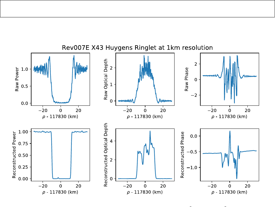
This run will produce a plot of the raw diffraction pattern, optical depth, and phase, as well as the
reconstructed power, optical depth, and phase. See Fig. 3below.
Fig. 3: Power, optical depth, and phase plots produced from Rev007EX43 HuygensRinglet test.py
3.4 End-to-end Pipeline: A Second Look at the Huygen’s Ringlet
The “end-to-end” pipeline process is a set of steps that need to be performed only once when processing
a given RSR file from scratch. For the initial run, users will need to supply an RSR file, a set of kernels
to use, a radial spacing to resample to, and a reconstruction resolution (there are also default keyword
inputs documented within each routine). The RSR extraction, geometry calculation, and frequency
offset calculation steps are all automated, but GUIs will appear for both calibration steps with initial
polynomial fits plotted. If these fits are not good enough, users can change which regions to fit and the
polynomial order using the GUI. Once this step has been done, pickle files are generated so that this
GUI-step does not need to be redone. Additionally, a text file of the calculated frequency offset is saved
so this time-consuming step does not need to be redone.
At the end of the end-to-end run, several data files will be generated: geometry files (GEO*.TAB
and GEO*.LBL), calibration files (FOF*.TXT, CAL*.TAB, CAL*.TAB, FRFP*.P, and PNFP*.P), a
diffraction-limited-profile file (DLP*.TAB), and an optical depth reconstruction file (TAU*.TAB). Each
class instantiated in the end-to-end pipeline process corresponds to a specific set of output files which
match those on the PDS. Once these files have been produced, users can use the quick-look process for
subsequent runs.
As a brief overview, an end-to-end script will require instantiating five separate Python classes in suc-
cession:
10

1. rsr inst = rss.RSRReader(‘RSR filename.a2a’)
•creates an instance of the RSRReader class and stores it in the variable rsr inst
2. geo inst = rss.occgeo.Geometry(rsr inst, ‘planet’, ‘spacecraft’, kernels)
•creates an instance of the Geometry class and stores it in the variable geo inst
•takes an RSRReader instance and user-specified planet, spacecraft, and kernel files
•calculates, among other things, the radial intercept point ρwhere the Cassini spacecraft radio
signal is occulted by the rings
•produces GEO*.TAB and GEO*.LBL files
•these and all subsequent output files are written to a user-specified output directory
3. cal inst = rss.calibration.Calibration(rsr inst,geo inst)
•creates an instance of the Calibration class and stores it in the variable cal inst
•takes the RSRReader (rsr inst) and Geometry (geom inst) instances
•this instance contains the calibrations necessary to convert the raw data into a diffraction-
limited radial ring profile
•calculates the observed frequency of the spacecraft signal to correct the real and imaginary
components of the transmittance (Iand Q), then estimates the intrinsic received power over
the entire occultation
•produces CAL*.TAB and CAL*.LBL files following the naming convention for the GEO files
4. dlp inst = rss.calibration.NormDiff(rsr inst,dr,geo inst,cal inst)
•creates an instance of the NormDiff class and stores it in the variable dlp inst
•takes the RSRReader,Geometry, and Calibration instances
•contains as attributes the DLP as calibrated and reduced by the previous classes
•optional input of radial sampling rate dr km desired in kilometers
•calculates the normalized power P/P0and the corresponding diffraction-limited optical depth
profile assuming τ=−sin Bln(P/P0)
•produces DLP*.TAB and DLP*.LBL files with the same naming convention as the GEO and
CAL files with the additional RRRR indicator
5. tau inst = rss.diffcorr.DiffractionCorrection(dlp inst,res km)
•creates an instance of the DiffractionCorrection class and stores it in the variable tau inst
•takes the NormDiff instance and a user-specified reconstruction resolution res km in kilometers
•calculates the optical depth profile with reconstruction by accounting for diffraction effects by
means of Fresnel inversion at the user-specified reconstruction resolution
•produces TAU*.TAB and TAU*.LBL files following the same naming convention as the DLP
files except that RRRR here indicates the reconstruction resolution selected by the user when
instantiating the DiffractionCorrection() class
As a demonstration of this end-to-end pipeline, we provide an example script which again examines the
Huygens ringlet, allowing users to compare their own end-to-end results to those produced by our test
script with provided geometry and calibration results. To execute this script, follow the example below.
host:∼user$ cd rss_ ringoc cs - master / exampl es
host:∼u se r$ p yth on e 2e _ru n . py
This will generate two successive GUIs. The first provides interactive polynomial fitting to the frequency
offset residuals, wherein the user may assess the quality of the polynomial fit, change the order of the
polynomial fit (default is ninth order), and optionally specify mask regions. The second provides inter-
active spline fitting to the power of the frequency-corrected spacecraft instrument when the spacecraft
is not being occulted by ring material (so-called free-space regions of the total occultation data set).
Predicted regions of free space are used in the initial fit and highlighted for the user. The user may
change the spline order (default is quadratic) and regions of free space interactively and assess the spline
results before continuing. Free space is selected in the same manner as the frequency offset residuals.
For details on use of the GUIs, see Appendices Band C.
11
3.5 Quick-Look Method: Comparing Profiles Reconstructed at Different
Resolutions
The quick look approach allows users to save computation time by utilizing pre-computed data files.
For these runs, users start directly at the Fresnel inversion step of the pipeline, provided they have a
set of GEO*.TAB,CAL*.TAB, and DLP*.TAB files. Users must specify the relative file path(s) and desired
*.TAB files to the tools.ExtractCSVData() class to create a DLP instance like the one instantiated
from calibration.NormDiff() in the end-to-end pipeline. This DLP instance can then be passed to
the diffcorr.DiffractionCorrection() class.
Continuing with the RSR file downloaded in Section 2.5, we provide an example script to demonstrate
diffraction-reconstructed optical depth profiles at different reconstruction resolutions for the Maxwell
Ringlet. Before running, users will need to open the script in a text editor and change the * file
variables to include the appropriate file names as a string after the pre-specified path. For the first set
of Rev007 files output by the e2e run.py script, this might resemble
da ta_dir = ’ ../ o utput / Re v007 /E / Re v0 07E_ RSS_2 005_ 12 3_X4 3_E / ’
geo_ file = data_dir + ’ R S S_2 0 05_1 23_X 43_E _ GEO _ 2018 0926 _ 000 1 . TAB ’
cal_ file = data_dir + ’ R S S_2 0 05_1 23_X 43_E _ CAL _ 2018 0926 _ 000 1 . TAB ’
dlp_ file = data_dir + ’ R S S_20 05_1 2 3_X 4 3_E_ D LP_ 0 100M _ 201 8 0926 _000 1 . TAB ’
To execute the example quick-look script, follow the example below
host:∼user$ cd rss_ ringoc cs - master / exampl es
host:∼u se r$ p yth on q ui ck _l oo k_ ru n . py
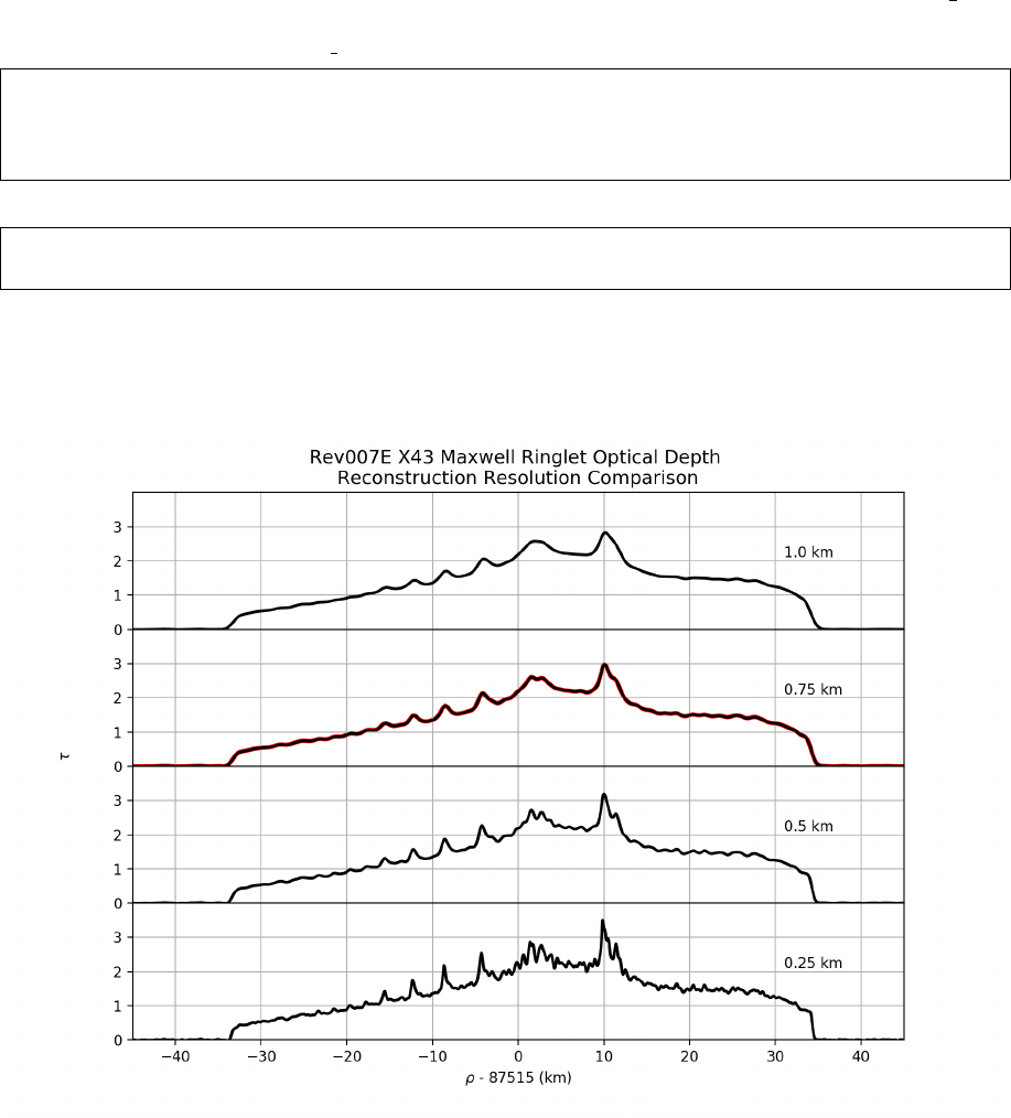
This will produce optical depth profiles at four different reconstruction resolutions: 1 km, 0.75 km, 0.5
km, and 0.25 km for the Rev007 egress X band observation processed by the end-to-end script in Section
3.4. Running the script as shown above will produce the plot in Figure 4.
Fig. 4: Optical depth profile for the Maxwell Ringlet from the Rev007E X43 occultation reconstructed at 1 km, 0.75 km, 0.5 km,
and 0.25 m resolution. Solid black lines are the optical depth profile produced by the quick-look example script at various processing
resolutions indicated by the plot text. For reference and validation, the solid red line is the 1 km reconstruction resolution profile
obtained from the PDS3.
12
4 A detailed look at the rss ringoccs software package
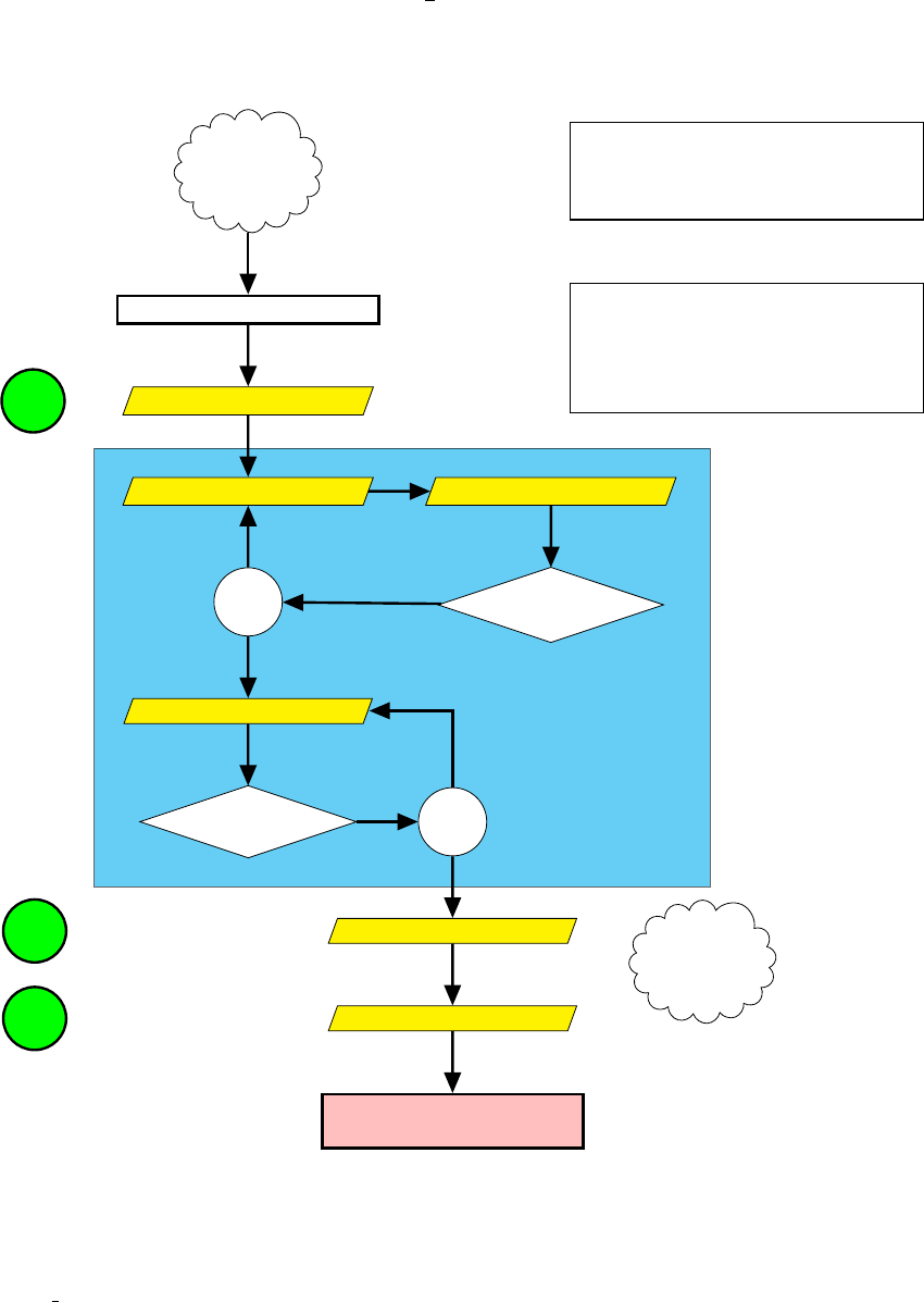
4.1 Pipeline Outline
End-to-End
RSR, Kernels
Geometry Calculation
*.Geo
Frequency Extraction Frequency Correction
Plot Frequencies
OK?
Power Normalization
Plot Power OK?
Norm. Diff. Pattern
*.Cal
Fresnel Inversion
*.Tau
Plots
Record of Script
Quick-Look
RSR Capabilities:
-Quickly Read Header
-Find Start/End SPM
-Read Records for Specified SPM Range
-Read Predicted Sky Frequency
Required Kernels:
-Spacecraft Ephemeris (SPK)
-Planetary Ephemeris (SPK)
-Planetary Constants (PCK)
-Leapseconds (LSK)
-Earth Stations (SPK)
-Earth Planetary Constants (PCK)
Calibration
No
Yes
No
Yes
Fig. 5: Data processing pipeline, with main steps in yellow, inputs in brackets above the main steps, files in bright green,
intermediate plots as white rhombuses, test conditions as white circles, and test decisions as red and green circles.
4.2 RSR Reader
The rsr reader/ subpackage is used for extracting information from a given RSR file. The RSRReader
class, when instantiated with a linked RSR file, extracts the raw complex signal Iand Qfrom the RSR
file from the PDS as well as some accompanying non-geometric meta data stored in the RSR file header
such as the DSN station, observation dates, sampling rate, start and end times of the observation, and
the band of observation.
13
4.3 Occultation geometry routines
The routines in occgeo/ depend heavily on the NAIF SPICE Toolkit and are geared towards repro-
ducing all occultation geometry parameters documented in the Cassini RSS Ring Profiles 2018 Archive
submission (see Table 3).
Symbol Parameter Name Geometry Attribute
tOET OBSERVED EVENT TIME t oet spm vals
tRET RING EVENT TIME t ret spm vals
tSET SPACECRAFT EVENT TIME t set spm vals
ρRING RADIUS rho km vals
φRL RING LONGITUDE phi rl deg vals
φORA OBSERVED RING AZIMUTH phi ora deg vals
BOBSERVED RING ELEVATION B deg vals
DSPACECRAFT TO RING INTERCEPT DISTANCE D km vals
Vrad RING INTERCEPT RADIAL VELOCITY rho dot kms vals
Vaz RING INTERCEPT AZIMUTHAL VELOCITY phi rl dot kms vals
FFRESNEL SCALE F km vals
Rimp IMPACT RADIUS R imp km vals
rxSPACECRAFT POSITION X rx km vals
rySPACECRAFT POSITION Y ry km vals
rzSPACECRAFT POSITIION Z rz km vals
vxSPACECRAFT VELOCITY X vx kms vals
vySPACECRAFT VELOCITY Y vy kms vals
vzSPACECRAFT VELOCITY Z vz kms vals
Table 3: Glossary of parameters in *GEO.TAB file in PDS submission Cassini RSS Ring Profiles 2018 Archive and their corre-
sponding attribute names within the Geometry class.
In addition to these parameters, Geometry also calculates the elevation angle of the observation at the
DSN station, the optical depth enhancement factor β, and the effective ring opening angle Beff .
To create an instance of Geometry, or geo inst, users will need an instance of the RSRReader class
(rsr inst), a target planet, a target spacecraft, a set of kernels over the duration of the RSR file used
in rsr inst, and, optionally, a desired number of points per seconds for all calculations (the default
is 1 point per second). For choosing an RSR file, which is the only input necessary for instantiating
RSRReader, see Section 5.2.
4.4 Calibration routines
All of the routines to produce a calibrated diffraction pattern are in the calibration/ directory in the
rss ringoccs package. Each of them performs a portion of the frequency and power calibration steps.
We will describe these routines in the order in which they are used.
The calc freq offset function calculates the frequency offset as a function of time. Its one mandatory
argument is an instance of the RSRReader class (rsr inst). Its optional inputs are dt freq for the time
spacing at which you want it to calculate frequency offset (default is 8.192 seconds; to avoid rounding
error, we suggest choosing a frequency offset that is a power of two, which is easily represented in binary),
cpu count for the number of CPU cores to use in multiprocessing (default is the number of CPU cores
on the user’s local machine), freq offset file for a string specifying where you want to store the text
file of saved values (defaults to None to save no file), and verbose for a Boolean specifying whether
to print out intermediate steps or results. To calculate frequency offset, we use numpy’s FFT class
to compute the frequency components of the raw measured complex signal for one time bin of width
dt freq.calc freq offset estimates the frequency corresponding to the peak in the power spectrum
near the center of the bandwidth by iteratively decreasing the frequency spacing and bin width. This
returns a final estimate for the frequency offset after three iterations.
14

Symbol Parameter Name Calibration Attribute
tOET OBSERVED EVENT TIME t oet spm vals
fsky SKY FREQUENCY rho corr pole km vals
fresid RESIDUAL FREQUENCY rho corr timing km vals
Pfree FREESPACE POWER tau norm vals
Table 4: Glossary of calibration data in the CAL files.
The FreqOffsetFit class fits a polynomial to the frequency offset calculated in the previous step. The
mandatory arguments are an instance of the RSRReader class (rsr inst), an instance of the Geometry
class (geo inst), the SPM and frequency offset output from the calc freq offset function (f spm
and f offset), and the USO frequency for the band of the RSR file (f uso). Its optional inputs are
poly order for the order of the polynomial fit (default of 9), spm include for the SPM regions to include
when making the fit (default of None to use hard-coded ring radius regions), sc name for the spacecraft
name (for now, always keep at the default of “Cassini”), USE GUI for a Boolean specifying whether or not
to use the GUI (default of True), and verbose for a Boolean specifying whether to print intermediate
steps or results to the command line. When an instance of the class is made, it calculates predicted and
reconstructed sky frequency, and calculates the residual frequency from these and the input frequency
offset. This portion uses the calc f sky recon function. The set f sky resid fit method of the class
has all the same optional inputs as the instantiation of the class except for sc name. This method calls
the GUI to make a fit by default, which uses the FResidFitGUI class. Any input in the GUI or with
the keywords in the command line will override the default fit. After making a satisfactory fit, there
is a method called get IQ c to get the frequency-corrected complex signal at raw resolution with the
corresponding set of SPM.
After frequency calibration, the Normalization class makes a spline fit to power in order to normalize
it to 1. In instantiation of the class, the mandatory arguments are raw resolution SPM and frequency-
corrected complex signal (spm raw and IQ c raw), an instance of the Geometry class (geo inst), and
an instance of the RSRReader class (rsr inst). The one optional keyword is verbose for a Boolean
specifying whether you want to print out intermediate steps or results. Calling the get spline fit
method returns a spline fit to power with corresponding SPM. The method downsamples raw-resolution
frequency-corrected complex signal, then makes a default fit to the resulting power using hard-coded
ring radius free-space regions and knots. This method also calls the GUI unless otherwise specified with
the USE GUI keyword, which calls the PowerFitGui class.
The Calibration class takes the results of the calibration processes and puts it into one place. It
creates an instance/object version of the CAL file. The mandatory arguments are an instance of the
FreqOffsetFit class (fit inst), an instance of the Normalization class (norm inst), and an instance
of the Geometry class (geo inst). The optional keywords are dt cal for the time spacing of the attributes
in the instance (default of 0.1 seconds), and verbose for a Boolean specifying whether you want to print
out intermediate steps or results. All this routine does is conglomerate the reuslts of the two calibration
steps into one place that is an instance version of the CAL file.
15

4.5 Diffraction-limited Profile Routines
Symbol Parameter Name NormDiff Attribute
ρRING RADIUS rho km vals
∆ρIP RADIUS CORRECTION DUE TO IMPROVED POLE rho corr pole km vals
∆ρT O RADIUS CORRECTION DUE TO TIMING OFFSET rho corr timing km vals
φRL RING LONGITUDE phi rl rad vals
φORA OBSERVED RING AZIMUTH phi ora rad vals
τNORMAL OPTICAL DEPTH tau norm vals
φPHASE SHIFT phase rad vals
τT H NORMAL OPTICAL DEPTH THRESHOLD tau threshold vals
tOET OBSERVED EVENT TIME t oet spm vals
tRET RING EVENT TIME t ret spm vals
tSET SPACECRAFT EVENT TIME t set spm vals
BOBSERVED RING ELEVATION B rad vals
Table 5: Glossary of optical depth, phase shift, and selected geometry parameters contained in the TAU files.
The NormDiff class takes the calibration results and produces a final frequency-calibrated, normalized
diffraction pattern resampled to uniformly-spaced ring radius. The mandatory arguments are an instance
of the RSRReader class (rsr inst), the radial spacing to which to resample (dr km), an instance of the
Geometry class (geo inst), and an instance of the Calibration class (cal inst). The optional keywords
are dr km tol for the maximum radius to be away from an even number of dr km (default of 0.01 km),
is chord to specify whether the occultation is a chord occultation (default of False), and verbose for a
Boolean specifying whether you want to print out intermediate steps or results. This routine assembles
everything needed for a DLP file, which involves resampling to uniform radius using the resample IQ
function. If it is a chord occultation, the chord split method will return two different instances of the
class, one for ingress and the other for egress. It is important to pass these instances one-by-one to the
diffraction reconstruction class: otherwise, rss ringoccs will quit because the diffraction reconstruction
cannot handle the calibrated data if dρ/dtcontains data with more than one sign.
4.6 Diffraction reconstruction routines
Symbol Parameter Name Attribute Name
∆RRECONSTRUCTION RESOLUTION (KM) res
ρRING RADIUS rho km vals
∆ρIP RADIUS CORRECTION DUE TO IMPROVED POLE rho corr pole km vals
∆ρT O RADIUS CORRECTION DUE TO TIMING OFFSET rho corr timing km vals
φRL RING LONGITUDE phi rl rad vals
φORA OBSERVED RING AZIMUTH phi rad vals
τNORMAL OPTICAL DEPTH tau vals
φPHASE SHIFT phase rad vals
τT H NORMAL OPTICAL DEPTH THRESHOLD tau threshold vals
tOET OBSERVED EVENT TIME t oet spm vals
tRET RING EVENT TIME t ret spm vals
tSET SPACECRAFT EVENT TIME t set spm vals
BOBSERVED RING ELEVATION B rad vals
wWINDOW WIDTH FOR RECONSTRUCTION w km vals
fsky SKY FREQUENCY f sky hz vals
FFRESNEL SCALE F km vals
DSPACECRAFT-RIP DISTANCE D km vals
ˆ
TDIFFRACTED COMPLEX TRANSMITTANCE T hat vals
TRECONSTRUCTED COMPLEX TRANSMITTANCE T vals
Table 6: Glossary of optical depth, phase shift, and selected geometry parameters contained in files CARL TAU 01KM.TAB and
RSS 2005 123 X43 E TAU 10KM.TAB. See companion label (.LBL) files for description of the data.
16
All of the diffraction reconstruction tools are located within the diffrec subpackage of rss ringoccs.
One can find simple tools for diffraction reconstruction of the diffraction pattern contained in an instance
of the NormDiff class, as well as more complex tools for modeling problems and comparing them with
real-world data and geometry. The main dependency is the numpy package, but some functions also rely
on tools found in the scipy package. The subpackage is broken into four submodules: advanced tools,
diffraction correction,special functions, and window functions.diffraction correction is
the primary tool and this contains the DiffractionCorrection class, which is the main utility for
creating diffraction-reconstructed profiles of radio occultation observations. The syntax is as follows:
In [1]: from r ss_ri ngo ccs import diffrec
In [ 2] : rec = diff rec . D if fr ac ti on Co rr ec tion ( no rm_i ns t , res )
Here, norm inst is an instance of the NormDiff class containing the diffracted data and res is the user-
requested processing resolution of the reconstructed profiles in kilometers and expressed as a floating
point number. There are several keywords in this class to allow the user to specify how the diffraction
reconstruction will be performed. Below is a brief description of the various keywords and arguments for
this class.
DiffractionCorrection Arguments
norm inst:
An instance of the NormDiff class which contains all of the necessary variables to
perform diffraction reconstruction. This includes the geometry of the occultation,
the diffracted raw power, and the phase.
res:
The user-requested resolution, specified in kilometers, of the reconstructed profiles.
This is a positive floating point number. It is bounded below by twice the sam-
ple spacing that is contained in the NormDiff class, in adherence to the sampling
theorem. Requests for smaller resolutions will produce an error message.
DiffractionCorrection Keywords
rng:
The requested ring plane radial range for diffraction reconstruction. This can be
either a list or a string, depending on the planet. Preferred inputs are lists of the
form rng = [a, b], where ais the (positive) inner limit to the radial range (in km) for
reconstruction, and bis the outer limit (again, in km). For Saturn, several regions
of interest are already specified and can be loaded in as strings. For example,
rng=“maxwell” is a valid input and will result in a reconstruction over the radial
range of the Maxwell ringlet: [87410,87610]. Currently acceptable strings are: ‘all’,
‘cringripples’, ‘encke’, ‘janusepimetheus’, ‘maxwell’, ‘titan’, ‘huygens’.
wtype:
A string specifying the requested window/tapering function to be applied during the
reconstruction process. By default a Kaiser-Bessel function with αparameter set
to 2.5 is used. The user may select any of the following: ‘rect’, ‘coss’, ‘kb20’, ‘kb25’,
‘kb35’, ‘kbmd20’, ‘kbmd25’, which stand for rectangular window, squared cosine
window, and various Kaiser-Bessel windows. The ‘kbmd’ windows are modified
versions of the Kaiser-Bessel functions. The standard ones do not tend to zero at the
edge of the window, but rather converge to 1/I0(απ), where I0is the modified Bessel
function. For large αthis is essentially zero, but for small values this discontinuity
in the window can cause unwanted fringe effects. The modification simply makes
the function zero at the edges, while still evaluating to 1 at the center.
fwd:
A Boolean for determining whether or not a forward calculation will be performed
at the end of reconstruction. If the reconstruction went well, this forward model
should match the data to the extent of smoothing effects caused by the finite positive
resolution that was requested. Default is set to False.
17

DiffractionCorrection Keywords (Cont.)
norm:
A Boolean for determining whether or not to normalize the reconstruction by the
window width. The reconstruction is defined as:
T(ρ) = 1−i
2FˆW/2
−W/2
ˆ
T(ρ0)w(ρ−ρ0)e−iψ(ρ,ρ0)dρ0,
where ˆ
Tis the diffracted data, exp(−iψ) is the Fresnel Kernel, wis the window
function, and Wis the window width. A quick look at this equation shows that as
the window width goes to zero, so does the reconstruction. That means for large
resolutions (10-km, or so), the reconstruction will be a small fraction of the input
data. To correct this we offer the ability to normalize the reconstruction by the
following factor:
N=´∞
−∞ eiψdρ
´W/2
−W/2weiψ dρ
Default is set to True.
bfac:
A Boolean for determining how to compute the window width about a particular
point. The standard definition of the window width is W= 2F2/∆R, where F
is the Fresnel Scale and ∆Ris the requested resolution. However, when the Allen
deviation is large, or when the velocity of ring intercept point (dρ/dt) is small, the
resolution is defined as:
∆R=2F2
W
b/2
exp(−b) + b−1,
where b=ω2σ2W/2 ˙ρ. Here, ωis the angular frequency, σis the Allen deviation,
and ˙ρis the ring intercept velocity. Solving for Wthen becomes a process of
inverting this equation, which requires the use of LambertW functions. Setting
bfac=True will compute the window width taking into account this “b” factor,
setting bfac=False uses the standard 2F2/∆R. Default is True.
sigma:
The Allen deviation. This is a positive floating point number. If bfac=False is set,
this parameter is ignored. See bfac for more documentation.
fft:
A Boolean for determining whether or not to use FFT’s for the computation. When
the Fresnel Kernel (see the equation listed under the “norm” keyword) is of the
form exp(iψ(ρ−ρ0)), the convolution theorem may be applied to compute the
reconstruction. This can greatly improve computation time. Default is False.
psitype:
A string that will determine how the Fresnel Kernel will be approximated (see the
equation listed under then “norm” keyword). Currently there are several options:
‘full’, ‘mtr2’, ‘mtr3’, ‘mtr4’, and ’fresnel’, none of which are case-sensitive. The MTR
options compute the polynomial approximations found in MTR86. “Full” uses no
approximation and ψwill be computed outright. “Fresnel” uses the classic quadratic
Fresnel approximation, which sets ψ=π
2(ρ−ρ0
F)2. Because of the simplicity of
the computation, ‘fresnel’ is by far the fastest in reconstruction time. For many
occultations, such as Cassini’s rev007, the difference between using ‘fresnel’ and
‘full’ is extremely small. For more pathological data sets, such as rev133, there are
severe differences. The user must be alert to note when various approximations are
valid. Default is psitype=‘full’.
write file:
A Boolean for determining if the *.TAU file will be written.
verbose:
Boolean for printing out status reports on the reconstruction. Default is False.
18

Below is a detailed description of the example included in the quick look run.py script discussed in
Section 3.5. As with the quick-look script itself, this example assumes that the user has available the req-
uisite *.TAB files generated by the example end-to-end script covered in Section 3.4. The ExtractCSVData
class covered in the next section can be used to extract information from the *.TAB files and reconstruct
the DLP instance norm inst.
In [ 1] : geo = " ../ Da ta / GEO . TAB "
In [ 2] : cal = " ../ Da ta / CAL . TAB "
In [ 3] : dlp = " ../ Da ta / DLP . TAB "
In [4]: from rs s_ri ngo ccs . tools import Ext rac tCSV Data
In [5]: from r ss_ri ngo ccs import diffrec
In [6]: no rm_inst = E xtr act CSV Dat a (geo , cal , dlp , verbose = False )
In [7]: ta u_i nst _f = diffrec . Dif frac tion Corr ectio n (
... : n or m_in st , 1.0 , rng = " all " , p sit ype = " fr esn el " )
Co mput ati on T ime : 12. 491 324
Note the quite short (12 second) reconstruction time, due in part to the ‘Fresnel’ setting for psitype and
1 km resolution. Running DiffractionCorrection with the default keywords, we find:
In [8]: ta u_i nst _v = diffrec . Dif frac tion Corr ectio n (data , 1.0 , verbose = True )
Things print out here ...
Co mput ati on T ime : 1 08. 427 886
In [9]: tau_ins t = di ff re c . Dif frac tio nCor rec tion ( data , 1.0)
Co mput ati on T ime : 76. 470 007
There are several things to note here. The default for psitype is ‘full’, and the computation of ψis one
of the slowest parts in the entire diffraction reconstruction algorithm. In particular, the computation of
the stationary phase (the value at which ∂ψ/∂φ = 0 – see MTR86) can be quite time-consuming. Since
‘Fresnel’ skips all of this, we see a substantial reduction in computation time. The data set that was
used in this example comes from the Cassini rev007E occultation observation. We can check the validity
of Fresnel approximation for this set by looking at the difference in the two reconstructions. Note that
since the power is normalized to 1, this is both fractional and absolute error:
In [10]: im port numpy as np
In [ 11]: np . max ( np . abs ( r ec f . pow er_val s - r ec . p owe r_ val s ))
Out [11]: 0 .00 0167 845 7 932 6811 766
In [ 12 ]: np . me an ( np . a bs ( r ec f . p owe r_v als - rec . p ow er _v al s ))
Out [12]: 3 .537 47 68 4013 31 293 e -06
The Fresnel approximation works very well here. Another thing to note is that there is a large discrepancy
in the computation time for when verbose=True and verbose=False is set. Since verbose prints out pieces
of information for every point that is being reconstructed, the Python interpreter needs to wait for the
line to be printed before it can process the next point. In most cases this is not an issue, but when speed
is crucial it may be better to leave verbose set to False.
4.7 Utility routines
Within our tools/ subpackage, we have provided several routines, the pds3 * series.py scripts, to
read and write PDS3-type data and label files.10 rss ringoccs manages the file naming conventions
and calling of the pds3 * series.py scripts by means of the write output files.py script. Another
utility in the subpackage, write intermediate files, creates three files relevant to the calibration step
of the end-to-end pipeline:
1. * FOF *.txt – an ascii text file that contains the initial estimates of the frequency offset found by
computationally expensive batches of FFTs
2. * FRFP *.P – a pickle binary file that contains a python dictionary of the coefficients of the poly-
nomial fit to the residual frequency offset
3. * PNFP * – a pickle binary file that contains the python dictionary of the B-spline coefficients of
the spline fit to the free space power
10The products of these routines have not been thoroughly checked for PDS3 compliance.
19

A separate tool built into the software as a keyword argument allows users to choose any one or pair
of pickle files to circumvent the GUI steps of the pipeline. The keyword file search can be set in the
calibration instance to read specific versions of one or both of the pickle files (most relevant if a user wants
to examine the change in the end product, the diffraction reconstructed optical depth profile, if, say, a
different spline or polynomial order is chosen or a different set of fit regions are selected). file search
can be set to None, one string with the appropriate relative path and pickle file name, or a list of two
strings specifying the relative path and names of both desired pickle files.
Also included as a utility for the quick-look pipeline is the ExtractCSVData, a tool for extracting in-
formation from the *.TAB files and reconstructing the DLP instance norm inst. This can be found in
the CSV tools submodule of the tools subpackage, all contained within rss ringoccs. The steps for
importing are shown below.
The ExtractCSVData imports user-specified *.TAB files produced by the end-to-end pipeline and uses
them to construct an instance of the NormDiff class that can then be passed on for diffraction recon-
struction as a part of the quick-look process. This way, the pipeline only needs to be run once on a
given data set, and then the user may experiment with different resolutions, window functions, etc., on
the diffracted data without repeated time consuming steps. For example, from the master directory of
rss ringoccs, one could use ipython to implement the following to construct a NormDiff instance from
*.TAB files output from a previous run:
Host:∼user$ cd ∼/Research/rss_ringoccs -master
Host:∼user$ ipython
In [ 1]: pa th = ’ ../ o ut put / Re v0 07 / E / R ev 0 07 E_ RS S _2 00 5_ 1 23 _X 43 _ E / ’
In [2]: geo = path+’RSS_2005_123_X43_E_GEO_20180926_0001.TAB’
In [3]: cal = path+’RSS_2005_123_X43_E_CAL_20180926_0001.TAB’
In [ 4]: dlp = pat h + ’ R SS _ 20 05 _ 12 3_ X 43 _E _ DL P_ 0 10 0M _ 20 18 0 92 6_ 0 00 1 . T AB ’
In [5]: from rs s_ri ngo ccs . tools import Ext rac tCSV Data
In [6]: from r ss_ri ngo ccs import diffrec
In [7]: no rm_inst = E xtr act CSV Dat a (geo , cal , dlp , verbose = True )
Ex tra cting Data from CSV Fi le s :
Ex tract ing Geo Data ...
Geo Data Compl et e .
Ex tract ing Cal Data ...
Cal Data Compl et e .
Ex tract ing DLP Data ...
DLP Data C om plete
Re triev ing Va riabl es ...
Co mp uting Varia bles ...
In ter pol ati ng Data ...
Data Extra cti on Compl ete .
Writing History...
History Com pl ete .
Extract CSV Data Com plete .
Note that it is possible to combine *.TAB files from different end-to-end runs of rss ringoccs, which is
encouraged for users who want to examine the effect different calibration inputs might have on the final
reconstructed optical depth profile.
5 Where To Go From Here
5.1 The Cassini RSS data catalog
We have created a CSV file, located within the tables directory, with all Cassini ring occultation RSR files
that we have on file. This catalog includes information of each RSR file, such as wavelength/frequency
band, observing station information, sampling rate, associated kernels, etc., as well as relevant geometry
parameters that can help users determine which file they want to use. The column headers and definitions
for this catalog are also available within the tables/ directory.
20

5.2 Selecting an RSR file to process
Before using rss ringoccs, we recommend users browse the Cassini RSS data catalog to find an appro-
priate RSR file to process. Factors such as elevation angle, antenna size, radius range, and ring opening
angle can affect this decision.
First, users should establish that the RSR file covers the radius range of interest. Some occultations,
such as chords, do not cover the entire ring system (see Figure 21.2.2). Secondly, depending on research
goal, users will want either a large or small ring opening angle. A large ring opening angle means that
the spacecraft signal has gone through less ring material, and a small ring opening angle means that the
signal has gone through more ring material. The latter is useful for tenuous features, such as some C-ring
density waves, and the former is useful for observing optically thick regions, such as the B-ring. Another
factor to consider is the Earth receiving station. Different stations will record in different bands (S-, X-,
or Ka-band) using different sized antennas (34m or 70m). The location of the DSN is also important,
as Cassini could be lower in the sky at one station but higher in the sky at another – this affects the
amount of atmosphere the signal must go through to reach the station. These station-related factors can
affect the overall SNR as well as the background power drift.
5.3 Benchmarks
We provide a script which performs a benchmark test for the user’s local machine. (This utilizes a 16
kHz resolution RSR file, which is more computationally expensive than the corresponding 1 kHz file, but
this file is not yet available on the PDS). To run the benchmarking script, follow the example here:
host:∼user$ cd rss_ ringoc cs - master / pipeli ne
host:∼u se r$ p yth on b e nc hm ar k_ te st . py
Team Cassini has conducted a series of benchmarks for various machines across a range of hardware and
operating systems. The results of these benchmark runs are listed below for reference:
∆Rres (km) ∆ρ(km) Hardware Total (sec)
1.0 0.25 MacBook Pro, 2.9 GHz Intel Core i7, 16GB RAM 493.9
1.0 0.25 MacBook Pro, 2.7 GHz Intel Core i5 8GB RAM 1032.4
0.5 0.25 MacBook Pro, 2.9 GHz Intel Core i7, 16GB RAM 547.7
0.5 0.25 MacBook Pro, 2.7 GHz Intel Core i5 8GB RAM 1200.2
0.25 0.05 MacBook Pro, 2.9 GHz Intel Core i7, 16GB RAM 1212.1
0.25 0.05 Macbook Pro, 2.7 GHz Intel Core i5 8GB RAM 2487.8
0.1 0.05 MacBook Pro, 2.9 GHz Intel Core i7, 16GB RAM 3115.4
Table 7: Benchmarks for the rev7E X43 16kHz file
5.4 Licensing
rss ringoccs is free/open-source software made available under the GNU General Public License. The
following license is included with the init .py files in the rss ringoccs software package:
Co pyright (C) 2018 Team Cassini
This program is free s of tware : you can r edi strib ute it and / or modify it
under the terms of the GNU General Public License as p ublis he d by the
Fr ee So ft wa re F ou nda tio n , ei the r ve rs ion 3 of the Li ce nse , or ( at yo ur
option ) any l ater version .
This p ro gr am is di strib uted in the hope that it will be useful ,
but WITHOUT ANY WA RR ANTY ; without even the im plied w arranty of
ME RCH ANT ABI LITY or FITNESS FOR A PARTI CULAR PURPOSE . See the GNU General
Public L icense for more details .
You should have receiv ed a copy of the GNU Gen er al P ublic License along
wit h this p rog ram . If not , see ht tp :// www . gnu . org / l ice nses /.
This program is part of the rss _ring occ s re posit ory hosted at
21

ht tp s :// g ith ub . com / NASA - Planeta ry - S cie nce / r ss_r in goc cs and de velo ped
with the f in ancia l s up po rt of NASA ’s Cas si ni Mission to Sa turn
Acknowledgements
Development of rss ringoccs was supported by NASA/JPL as part of the Cassini Mission Closeout
effort. The authors especially appreciate the support and encouragement of Linda Spilker and Kathryn
Weld. We dedicate this work to the memory of Arv Kliore, the original Cassini RSS Team Leader and
an example of wisdom and kindness for us all.
22

Appendix
A Meta Kernel File
An example meta kernel Rev007 meta kernel has been provided in the ./examples/ directory for the
Rev007 occultations. To create a meta kernel for another occultation, follow the structure of the Rev007
meta kernel example. Typically, the only files one needs to change are those with a *.bsp or *.tpc
extension. All kernel files necessary for building the meta kernel for a specific observation are listed in
final column of the data catalog found in the /tables/ directory. For example, the Rev014 occultation
would have a meta kernel
\ be gi ndata
PA TH_ VAL UES = ( ’../ kerne ls / naif / CA SSINI / kernels / spk ’
’../ kernels / naif / CASSINI / kernels /lsk ’
’../ ke rn el s / naif / gen eri c_k ern els / spk / planets ’
’../ k ernels / nai f/ g ene ri c_ke rnel s / spk / station s ’
’../ ke rn el s / naif / gen eri c_k ern els / pck ’
’../ kernels / naif / CASSINI / kernels /pck ’
’../ ke rn els / local ’)
P AT H_ SY MB OL S = ( ’A ’ , ’B ’ , ’C ’ , ’D ’ , ’E ’ , ’F ’ , ’G ’)
KE RNE LS_ TO_ LOA D = ( ’$A /051011 R _SCP SE_ 052 45_0 525 7 . bsp ’
’ $B / n ai f00 12 . tls ’
’$C / de 43 0 .bsp ’
’F / cpc k11 Oct2005 . tpc ’
’$D / ea rths tns _itr f93_ 050 714 .bsp ’
’$F/earth_000101_180919_180629.bpc’)
\ be gi ntext
these are the k er ne ls used for Rev014
B Frequency Offset Fitting GUI
The Calibration instance will draw the GUI shown below when performing the polynomial fit to the
frequency offset residuals as a part of the correction to the observed Iand Q. The user may change the
polynomial order using a dropdown widget to select an order anywhere from 2 to 9. The default order
is 9; however, the dropdown widget will display the number 3 when the GUI is first instantiated. Data
which have been excluded by sigma clipping (and are, ergo, excluded from the initial fitting procedure)
are shown in grey while data satisfying the sigma-clipping and occultation requirements are shown in
black. The line of best fit is shown in solid red.
23
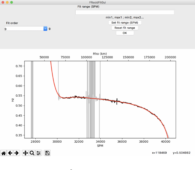
Fig. 6: The GUI which enables users to interactively fit the frequency offset residual. Shown in the plotting frame is the frequency
offset residual for Rev007E as processed by the e2e run.py script discussed in Section 3.4.
To include select regions of the frequency offset residual, enter the minimum and maximum seconds-
past-midnight of each region to be included in the fit with a comma delimiter. Then delimit between the
regions with a semicolon. For instance, to include only the regions of 30,000 to 32,000 SPM and 35,000
to 40,000 SPM, one would enter
30000,32000;35000,40000
into the “Fit range (SPM)” field.
C Free Space Power Fitting
The Calibration instance will create a GUI as shown below for the purpose of interactively fitting
the free-space power as a part of the power normalization process required to compute the diffraction-
limited profile. The power is normalized to the maximum power in the radial profile and is shown in
black. Initial approximations of the free space regions are shaded in grey; these are the regions which
are used to compute the initial spline approximation and are intended as a reference for the user. Spline
fit approximation of the power profile is shown in solid red.
24

Fig. 7: The GUI which enables users to interactively fit the free-space power signal. Shown in the plotting frame is the power
profile for Rev007E normalized to the maximum power observed as processed by the e2e run.py script discussed in Section 3.4.
Region masking for inclusion in the fit is done in the same manner as the frequency offset fitting. We
suggest knots for the spline fit be the midpoint between the minimum and maximum SPM of each region
of free space. Only one knot can be entered per free-space region and knot values are delimited by
commas. For the example in Figure 7, the knot entry might resemble
30500,31785,34080,34245,35285,36000
The apparent free space region to the far left of the profile that is excluded from the predicted free space
is signal occulted by Saturn’s ionosphere and is thus less reliable as an indicator of the intrinsic power.
It is suggested that users not include this part of the profile in the free space mask regions for calibrating
the normalized power.
25
Glossary
Atmospheric occultation Disappearance or reappearance of a source after
the signal has passed through the atmosphere of
a planet or satellite. 2
Chord occultation Ring occultation. 2
Deep Space Network NASA’s complex of Earth-based antennas, used
to communicate with spacecraft. 1
Diametric occultation An occultation geometry in which the path of
the complete occultation extends from ring ansa
to ring ansa, passing behind the planet at mid-
occultation.. 2
Diffraction Reconstruction Retrieval of radial optical depth profile of Sat-
urn’s rings responsible for observed diffraction
pattern. 1
Diffraction-limited profile Radial optical depth profile without correcting
for the effects . 3
Egress Exit phase of a ring or atmosphere occultation.
2
Fresnel inversion Retrieval of intrinsic optical depth profile of the
rings by using a Fresnel transform to correct for
the effects of diffraction in the observed signal.
1
High Gain Antenna Highly directional main spacecraft antenna for
communications and radio science. 1
Ingress Entry phase of a ring or atmosphere occultation.
2
NASA National Aeronautics and Space Administra-
tion. 1
Planetary Data System Long-term archive of digital data products re-
turned from NASA’s planetary missions, and
from other kinds of flight and ground-based data
acquisitions. 1
Radio Science Receiver An open-loop receiver used in NASA’s Deep
Space Network (DSN) facilities. 2,4,9
Radio Science Subsystem A subsystem placed on board a spacecraft for
radio science purposes. 1
Rev number The number of times the Cassini spacecraft has
orbited Saturn. 2
27
References
Acton, C. (1996), ‘Ancillary Data Services of NASA’s Navigation and Ancillary Information Facility’,
Planetary and Space Science 44, 65–70.
Colwell, J., Nicholson, P., Tiscareno, M., Murray, C., French, R. & Marouf, E. (2009), ‘The Structure of
Saturn’s Rings’, Saturn from Cassini-Huygens p. 375.
French, R., McGhee-French, C., Lonergan, K., Sepersky, T., Jacobson, R., Nicholson, P., Hedman, M.,
Marouf, E. & Colwell, J. (2017), ‘Noncircular features in Saturn’s rings IV: Absolute radius scale and
Saturn’s pole direction’, Icarus 290, 14–45.
French, R., Nicholson, P., Hedman, M., Hahn, J., McGhee-French, C., Colwell, J., Marouf, E. & Rappa-
port, N. (2016a), ‘Deciphering the embedded wave in Saturn’s Maxwell ringlet’, Icarus 279, 62–77.
French, R., Nicholson, P., McGhee-French, C., Lonergan, K., Sepersky, T., Hedman, M., Marouf, E. &
Colwell, J. (2016b), ‘Noncircular features in Saturn’s rings III: The Cassini Division’, Icarus 274, 131–
162.
Kliore, A., Anderson, J., Armstrong, J., Asmar, S., Hamilton, C., Rappaport, N., Wahlquist, H., Am-
brosini, R., Flasar, F., French, R., Iess, L., Marouf, E. & Nagy, A. (2004), ‘Cassini Radio Science’,
Space Science Reviews 115, 1–70.
Marouf, E., French, R., Rappaport, N., Wong, K., McGhee-French, C. & Anabtawi, A. (2011), ‘Uncov-
ering of small-scale quasi-periodic structure in Saturn’s ring C and possible origin’, EPSC-DPS Joint
Meeting 265.
Marouf, E., Tyler, L. & Rosen, P. (1986), ‘Profiling Saturn’s rings by radio occultation’, Icarus 68, 120–
166.
Moutamid, M. E., Nicholson, P., French, R., Tiscareno, M., Murray, C., Evans, M., French, C., Hedman,
M. & Burns, J. (2016), ‘How Janus’ orbital swap affects the edge of Saturn’s A ring?’, Icarus 279, 125–
140.
Nicholson, P., French, R. & Colwell, M. H. E. M. J. (2014a), ‘Noncircular features in Saturn’s rings I:
The edge of the B ring’, Icarus 227, 152–175.
Nicholson, P., French, R., McGhee-French, C., Hedman, M., Marouf, E., Colwell, J., Lonergan, K. &
Sepersky, T. (2014b), ‘Noncircular features in Saturn’s rings II: The C ring’, Icarus 241, 373–396.
Rappaport, N., Longaretti, P., French, R., Marouf, E. & McGhee, C. (2009), ‘A procedure to analyze
nonlinear density waves in Saturn’s rings using several occultation profiles’, Icarus 199.
Thomson, F., Marouf, E., Tyler, G., French, R. & Rappoport, N. (2007), ‘Periodic microstructure in
Saturn’s rings A and B’, Geophysical Research Letters 34, L23203.
28
