Saurav Kaushik Beginners Guide On Web Scraping In R With Hands Example

saurav_kaushik__beginners_guide_on_web_scraping_in_r_with_hands-on_example

User Manual:

Open the PDF directly: View PDF .
Page Count: 16

March 26, 2017

Beginner’s Guide on Web Scraping in R (using rvest) with hands-on

example

analyticsvidhya.com/blog/2017/03/beginners-guide-on-web-scraping-in-r-using-rvest-with-hands-on-knowledge

Saurav Kaushik , March 27, 2017 / 23

Introduction

Data and information on the web isgrowing exponentially. All of us today use Google as our first source of

knowledge – be it about finding reviews about a place to understanding a new term. All this information is

available on the web already.

With the amount of data available over the web, it opens newhorizons of possibility for a Data Scientist. I

strongly believe web scrapping is a must have skill for any data scientist. In today’s world, all the data that you

need is already available on theinternet, the only thing limiting you from using it is the ability to access it. With

the help of this article, you will be able to overcome that barrier as well.

Most of the data available over the webis not readily available. It is present in an unstructured format (HTML

format) and is not downloadable. Therefore, it requires knowledge & expertise to use this data.

In this article, I am going to take you through the process of web scrapping in R. With this article, you will gain

expertise to use any type of data available over the internet.

1. What is Web Scraping?

Web scraping is a technique for converting the data present in unstructured format (HTML tags) over the web

to the structured format which can easily be accessed and used.

Almost all the main languages provide ways for performing web scrapping. In this article, we’ll use R for

scrapping the data for the most popular feature films of 2016 from the IMDb website.

We’ll get a number of features for each of the 100 popular feature films released in 2016. Also, we’ll look at the

most common problems that one might face while scrapping data from theinternet because of lack of

consistency in the website code and look at how to solve these problems.

If you are more comfortable using Python, I’ll recommend you to go through this guide for getting started

with web scraping using Python.

2. Why do we need Web Scraping?

I am sure the first questions that must have popped in your headtill now is “Why do we need web scraping”?

As I stated before, the possibilities with web scraping are immense.

To provide you with hands-on knowledge, we are going to scrap data from IMDB. Some other possible

applications that you can use web scrapping for are:

Scrapping movie rating data to create movie recommendation engines.

Scrapping text data from Wikipedia and other sources for making NLP-based systems or training deep

learning models for tasks like topic recognition from the given text.

Scrapping labeled image data from websites like Google, Flickr, etc to train image classification models.

Scrapping data from social media sites like Facebook and Twitter for performing tasks Sentiment

analysis, opinion mining, etc.

Scrapping user reviews and feedbacks from e-commerce sites like Amazon, Flipkart, etc.

3. Ways to scrap data

There are several ways of scraping data from theweb. Some of the popular ways are:

Human Copy-Paste: This is a slow and efficient way of scraping data from theweb. This involves

humans themselves analyzing and copying the data to local storage.

Text pattern matching: Another simple yet powerful approach to extract information from theweb is

by using regular expression matching facilities of programming languages. You can learn more about

regular expressions here.

API Interface: Many websites like Facebook, Twitter, LinkedIn, etc. provides public and/ or private APIs

which can be called using standard code for retrieving the data in the prescribed format.

DOM Parsing: By using the web browsers, programs can retrieve the dynamic content generated by

client-side scripts. It is also possible to parse web pages into a DOM tree, based on which programs can

retrieve parts of these pages.

We’ll use the DOM parsing approach during the course of this article. And rely on the CSS selectors of the

webpage for finding the relevant fields which contain the desired information. But before we begin there are a

few prerequisites that one need in order to proficiently scrap data from any website.

4. Pre-requisites

The prerequisites for performing web scraping in R are divided into two buckets:

To get started with web scraping, you must have a working knowledge of R language. If you are just

starting or want to brush up the basics, I’ll highly recommend following this learning path in R. During

the course of this article, we’ll be using the ‘rvest’ package in R authored by Hadley Wickham. You can

access the documentation for rvest package here. Make sure you have this package installed. If you

don’t have this package by now, you can follow the following code to install it.

install.packages('rvest')

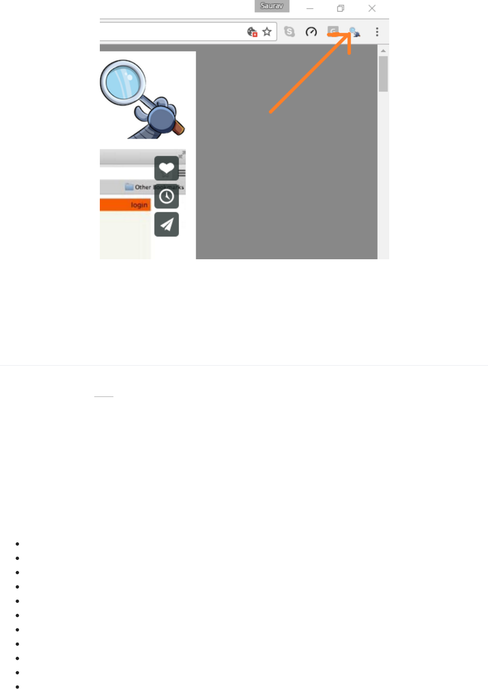
Adding, knowledge of HTML and CSS will be an added advantage. One of the best sources I could find

for learning HTML and CSS is this. I have observed that most of the Data Scientists are not very sound

with technical knowledge of HTML and CSS. Therefore, we’ll be using an open source software named

Selector Gadget which will be more than sufficient for anyone in order to perform Web scrapping. You

can access and download the Selector Gadget extension here. Make sure that you have this extension

installed by following the instructions from the website. I have done the same. I’m using Google chrome

and I can access the extension in the extension bar to the top right.

Using this you can select the parts of any website and get the relevant tags to get access to that part by simply

clicking on that part of the website. Note that, this is a way around to actually learning HTML & CSS and doing

it manually. But to master the art of Web scrapping, I’ll highly recommend you to learn HTML & CSS in order

to better understand and appreciate what’s happening under the hood.

4. Scraping a webpage using R

Now, let’s get started with scraping the IMDb website for the 100 most popular feature films released in 2016.

You can access them here.

#Loading the rvest package

library('rvest')

#Specifying the url for desired website to be scrapped

url <- 'http://www.imdb.com/search/title?count=100&release_date=2016,2016&title_type=feature'

#Reading the HTML code from the website

webpage <- read_html(url)

Now, we’ll be scraping the following data from this website.

Rank: The rank of the film from 1 to 100 on the list of 100 most popular feature films released in 2016.

Title: The title of the feature film.

Description: The description of the feature film.

Runtime: The duration of the feature film.

Genre: The genre of the feature film,

Rating: The IMDb rating of the feature film.

Metascore: The metascore on IMDb website for the feature film.

Votes:Votes cast in favor of the feature film.

Gross_Earning_in_Mil: The gross earnings of the feature film in millions.

Director: The main director of the feature film. Note, in case of multiple directors, I’ll take only the first.

Actor: The main actor of the feature film. Note, in case of multiple actors, I’ll take only the first.

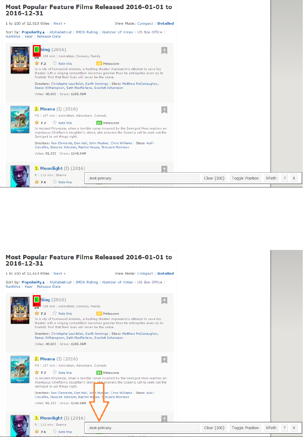
Here’s a screenshot that contains how all these fields are arranged.

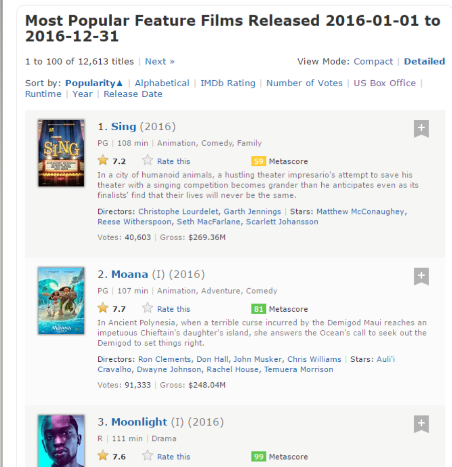
Step 1: Now, we will start with scraping the Rank field. For that, we’ll use the selector gadget to get the specific

CSS selectors that encloses the rankings. You can click on the extenstion in your browser and select the

rankings field with cursor.

Make sure that all the rankings are selected. You can select some more ranking sections in case you are not

able to get all of them and you can also de-select them by clicking on the selected section to make sure that

you only have those sections highlighted that you want to scrap for that go.

Step 2: Once you are sure that you have made the right selections, you need to copy the corresponding CSS

selector that you can view in the bottom center.

Step 3: Once you know the CSS selector that contains the rankings, you can use this simple R code to get all

the rankings:

#Using CSS selectors to scrap the rankings section

rank_data_html <- html_nodes(webpage,'.text-primary')

#Converting the ranking data to text

rank_data <- html_text(rank_data_html)

#Let's have a look at the rankings

head(rank_data)

[1] "1." "2." "3." "4." "5." "6."

Step 4: Once you have the data, make sure that it looks in the desired format. I am preprocessing my data to

convert it to numerical format.

#Data-Preprocessing: Converting rankings to numerical

rank_data<-as.numeric(rank_data)

#Let's have another look at the rankings

head(rank_data)

[1] 1 2 3 4 5 6

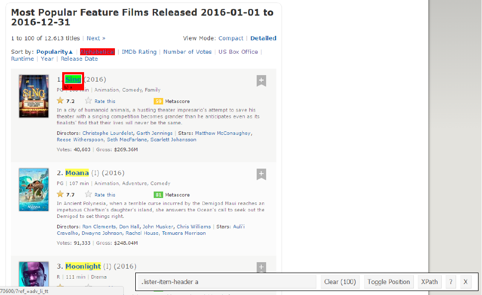
Step 5: Now you can clear the selector section and select all the titles. You can visually inspect that all the titles

are selected. Make any required additions and deletions with the help of your curser. I have done the same

here.

Step 6: Again, I have the corresponding CSS selector for the titles – .lister-item-header a. I will use this selector

to scrap all the titles using the following code.

#Using CSS selectors to scrap the title section

title_data_html <- html_nodes(webpage,'.lister-item-header a')

#Converting the title data to text

title_data <- html_text(title_data_html)

#Let's have a look at the title

head(title_data)

[1] "Sing" "Moana" "Moonlight" "Hacksaw Ridge"

[5] "Passengers" "Trolls"

Step 7: In the following code, I have done the same thing for scrapping – Description, Runtime, Genre, Rating,

Metascore, Votes, Gross_Earning_in_Mil , Director and Actor data.

#Using CSS selectors to scrap the description section

description_data_html <- html_nodes(webpage,'.ratings-bar+ .text-muted')

#Converting the description data to text

description_data <- html_text(description_data_html)

#Let's have a look at the description data

head(description_data)

[1] "\nIn a city of humanoid animals, a hustling theater impresario's attempt to save his theater with a

singing competition becomes grander than he anticipates even as its finalists' find that their lives will never

be the same."

[2] "\nIn Ancient Polynesia, when a terrible curse incurred by the Demigod Maui reaches an impetuous

Chieftain's daughter's island, she answers the Ocean's call to seek out the Demigod to set things right."

[3] "\nA chronicle of the childhood, adolescence and burgeoning adulthood of a young, African-American, gay man

growing up in a rough neighborhood of Miami."

[4] "\nWWII American Army Medic Desmond T. Doss, who served during the Battle of Okinawa, refuses to kill

people, and becomes the first man in American history to receive the Medal of Honor without firing a shot."

[5] "\nA spacecraft traveling to a distant colony planet and transporting thousands of people has a malfunction

in its sleep chambers. As a result, two passengers are awakened 90 years early."

[6] "\nAfter the Bergens invade Troll Village, Poppy, the happiest Troll ever born, and the curmudgeonly Branch

set off on a journey to rescue her friends.

#Data-Preprocessing: removing '\n'

description_data<-gsub("\n","",description_data)

#Let's have another look at the description data

head(description_data)

[1] "In a city of humanoid animals, a hustling theater impresario's attempt to save his theater with a singing

competition becomes grander than he anticipates even as its finalists' find that their lives will never be the

same."

[2] "In Ancient Polynesia, when a terrible curse incurred by the Demigod Maui reaches an impetuous Chieftain's

daughter's island, she answers the Ocean's call to seek out the Demigod to set things right."

[3] "A chronicle of the childhood, adolescence and burgeoning adulthood of a young, African-American, gay man

growing up in a rough neighborhood of Miami."

[4] "WWII American Army Medic Desmond T. Doss, who served during the Battle of Okinawa, refuses to kill people,

and becomes the first man in American history to receive the Medal of Honor without firing a shot."

[5] "A spacecraft traveling to a distant colony planet and transporting thousands of people has a malfunction

in its sleep chambers. As a result, two passengers are awakened 90 years early."

[6] "After the Bergens invade Troll Village, Poppy, the happiest Troll ever born, and the curmudgeonly Branch

set off on a journey to rescue her friends."

#Using CSS selectors to scrap the Movie runtime section

runtime_data_html <- html_nodes(webpage,'.text-muted .runtime')

#Converting the runtime data to text

runtime_data <- html_text(runtime_data_html)

#Let's have a look at the runtime

head(runtime_data)

[1] "108 min" "107 min" "111 min" "139 min" "116 min" "92 min"

#Data-Preprocessing: removing mins and converting it to numerical

runtime_data<-gsub(" min","",runtime_data)

runtime_data<-as.numeric(runtime_data)

#Let's have another look at the runtime data

head(rank_data)

[1] 1 2 3 4 5 6

#Using CSS selectors to scrap the Movie genre section

genre_data_html <- html_nodes(webpage,'.genre')

#Converting the genre data to text

genre_data <- html_text(genre_data_html)

#Let's have a look at the runtime

head(genre_data)

[1] "\nAnimation, Comedy, Family "

[2] "\nAnimation, Adventure, Comedy "

[3] "\nDrama "

[4] "\nBiography, Drama, History "

[5] "\nAdventure, Drama, Romance "

[6] "\nAnimation, Adventure, Comedy "

#Data-Preprocessing: removing \n

genre_data<-gsub("\n","",genre_data)

#Data-Preprocessing: removing excess spaces

genre_data<-gsub(" ","",genre_data)

#taking only the first genre of each movie

genre_data<-gsub(",.*","",genre_data)

#Convering each genre from text to factor

genre_data<-as.factor(genre_data)

#Let's have another look at the genre data

head(genre_data)

[1] Animation Animation Drama Biography Adventure Animation

10 Levels: Action Adventure Animation Biography Comedy Crime Drama ... Thriller

#Using CSS selectors to scrap the IMDB rating section

rating_data_html <- html_nodes(webpage,'.ratings-imdb-rating strong')

#Converting the ratings data to text

rating_data <- html_text(rating_data_html)

#Let's have a look at the ratings

head(rating_data)

[1] "7.2" "7.7" "7.6" "8.2" "7.0" "6.5"

#Data-Preprocessing: converting ratings to numerical

rating_data<-as.numeric(rating_data)

#Let's have another look at the ratings data

head(rating_data)

[1] 7.2 7.7 7.6 8.2 7.0 6.5

#Using CSS selectors to scrap the votes section

votes_data_html <- html_nodes(webpage,'.sort-num_votes-visible span:nth-child(2)')

#Converting the votes data to text

votes_data <- html_text(votes_data_html)

#Let's have a look at the votes data

head(votes_data)

[1] "40,603" "91,333" "112,609" "177,229" "148,467" "32,497"

#Data-Preprocessing: removing commas

votes_data<-gsub(",","",votes_data)

#Data-Preprocessing: converting votes to numerical

votes_data<-as.numeric(votes_data)

#Let's have another look at the votes data

head(votes_data)

[1] 40603 91333 112609 177229 148467 32497

#Using CSS selectors to scrap the directors section

directors_data_html <- html_nodes(webpage,'.text-muted+ p a:nth-child(1)')

#Converting the directors data to text

directors_data <- html_text(directors_data_html)

#Let's have a look at the directors data

head(directors_data)

[1] "Christophe Lourdelet" "Ron Clements" "Barry Jenkins"

[4] "Mel Gibson" "Morten Tyldum" "Walt Dohrn"

#Data-Preprocessing: converting directors data into factors

directors_data<-as.factor(directors_data)

#Using CSS selectors to scrap the actors section

actors_data_html <- html_nodes(webpage,'.lister-item-content .ghost+ a')

#Converting the gross actors data to text

actors_data <- html_text(actors_data_html)

#Let's have a look at the actors data

head(actors_data)

[1] "Matthew McConaughey" "Auli'i Cravalho" "Mahershala Ali"

[4] "Andrew Garfield" "Jennifer Lawrence" "Anna Kendrick"

#Data-Preprocessing: converting actors data into factors

actors_data<-as.factor(actors_data)

But, I want you to closely follow what happens when I do the same thing for Metascore data.

#Using CSS selectors to scrap the metascore section

metascore_data_html <- html_nodes(webpage,'.metascore')

#Converting the runtime data to text

metascore_data <- html_text(metascore_data_html)

#Let's have a look at the metascore

data head(metascore_data)

[1] "59 " "81 " "99 " "71 " "41 "

[6] "56 "

#Data-Preprocessing: removing extra space in metascore

metascore_data<-gsub(" ","",metascore_data)

#Lets check the length of metascore data

length(metascore_data)

[1] 96

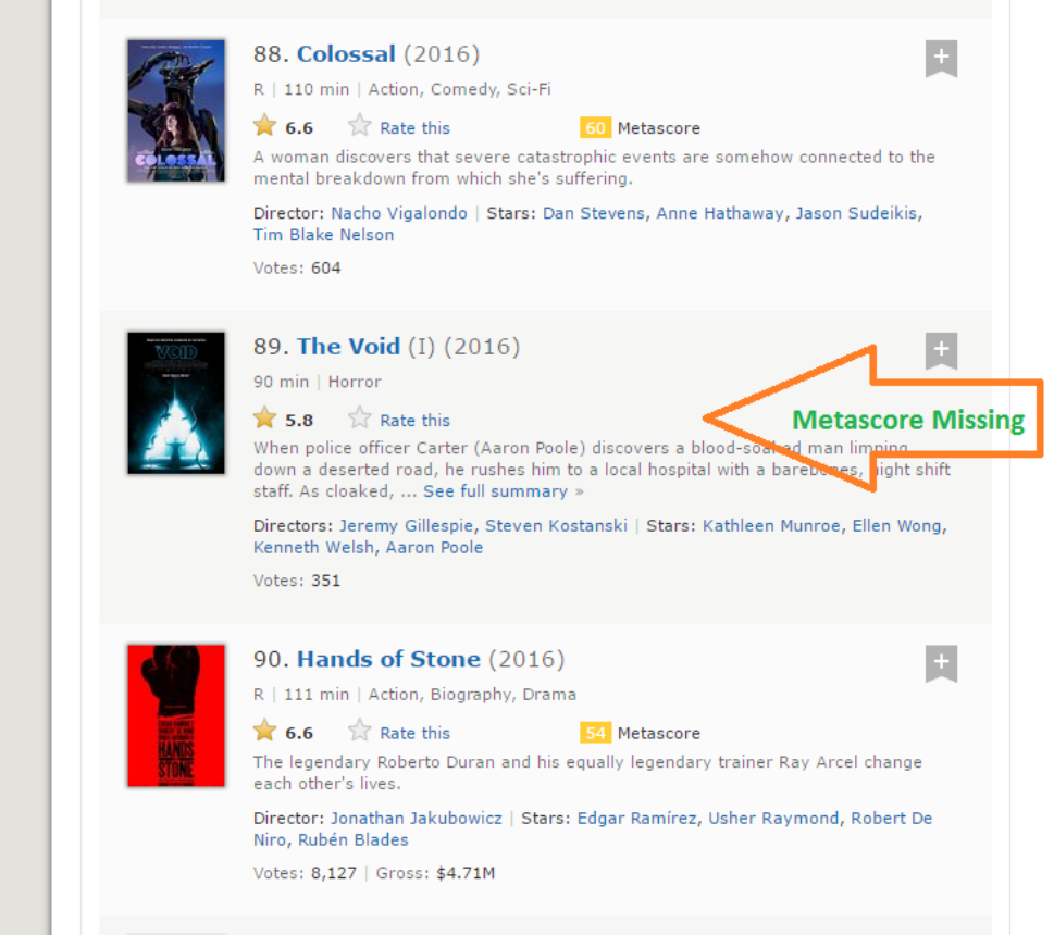
Step 8: The length of meta score data is 96 while we are scrapping the data for 100 movies. The reason this

happened is because there are 4 movies which don’t have the corresponding Metascore fields.

Step 9: It is a practical situation which can arise while scrapping any website. Unfortunately, if we simply add

NA’s to last 4 entries, it will map NA as Metascore for movies 96 to 100 while in reality, the data is missing for

some other movies. After a visual inspection, I found that the Metascore is missing for movies 39, 73, 80 and

89. I have written the following function to get around this problem.

for (i in c(39,73,80,89)){

a<-metascore_data[1:(i-1)]

b<-metascore_data[i:length(metascore_data)]

metascore_data<-append(a,list("NA"))

metascore_data<-append(metascore_data,b)

}

#Data-Preprocessing: converting metascore to numerical

metascore_data<-as.numeric(metascore_data)

#Let's have another look at length of the metascore data

length(metascore_data)

[1] 100

#Let's look at summary statistics

summary(metascore_data)

Min. 1st Qu. Median Mean 3rd Qu. Max. NA's

23.00 47.00 60.00 60.22 74.00 99.00 4

Step 10: The same thing happens with the Gross variable which represents gross earnings of that movie in

millions. I have use the same solution to work my way around:

#Using CSS selectors to scrap the gross revenue section

gross_data_html <- html_nodes(webpage,'.ghost~ .text-muted+ span')

#Converting the gross revenue data to text

gross_data <- html_text(gross_data_html)

#Let's have a look at the votes data

head(gross_data)

[1] "$269.36M" "$248.04M" "$27.50M" "$67.12M" "$99.47M" "$153.67M"

#Data-Preprocessing: removing '$' and 'M' signs

gross_data<-gsub("M","",gross_data)

gross_data<-substring(gross_data,2,6)

#Let's check the length of gross data

length(gross_data)

[1] 86

#Filling missing entries with NA

for (i in c(17,39,49,52,57,64,66,73,76,77,80,87,88,89)){

a<-gross_data[1:(i-1)]

b<-gross_data[i:length(gross_data)]

gross_data<-append(a,list("NA"))

gross_data<-append(gross_data,b)

}

#Data-Preprocessing: converting gross to numerical

gross_data<-as.numeric(gross_data)

#Let's have another look at the length of gross data

length(gross_data)

[1] 100

summary(gross_data)

Min. 1st Qu. Median Mean 3rd Qu. Max. NA's

0.08 15.52 54.69 96.91 119.50 530.70 14

Step 11: Now we have successfully scrapped all the 11 features for the 100 most popular feature films released

in 2016. Let’s combine them to create a dataframe and inspect its structure.

#Combining all the lists to form a data frame

movies_df<-data.frame(Rank = rank_data, Title = title_data,

Description = description_data, Runtime = runtime_data,

Genre = genre_data, Rating = rating_data,

Metascore = metascore_data, Votes = votes_data,

Gross_Earning_in_Mil = gross_data,

Director = directors_data, Actor = actors_data)

#Structure of the data frame

str(movies_df)

'data.frame': 100 obs. of 11 variables:

$ Rank : num 1 2 3 4 5 6 7 8 9 10 ...

$ Title : Factor w/ 99 levels "10 Cloverfield Lane",..: 66 53 54 32 58 93 8 43 97 7 ...

$ Description : Factor w/ 100 levels "19-year-old Billy Lynn is brought home for a victory tour after a

harrowing Iraq battle. Through flashbacks the film shows what"| __truncated__,..: 57 59 3 100 21 33 90 14 13 97

...

$ Runtime : num 108 107 111 139 116 92 115 128 111 116 ...

$ Genre : Factor w/ 10 levels "Action","Adventure",..: 3 3 7 4 2 3 1 5 5 7 ...

$ Rating : num 7.2 7.7 7.6 8.2 7 6.5 6.1 8.4 6.3 8 ...

$ Metascore : num 59 81 99 71 41 56 36 93 39 81 ...

$ Votes : num 40603 91333 112609 177229 148467 ...

$ Gross_Earning_in_Mil: num 269.3 248 27.5 67.1 99.5 ...

$ Director : Factor w/ 98 levels "Andrew Stanton",..: 17 80 9 64 67 95 56 19 49 28 ...

$ Actor : Factor w/ 86 levels "Aaron Eckhart",..: 59 7 56 5 42 6 64 71 86 3 ...

You have now successfully scrapped the IMDb website for the 100 most popular feature films released in 2016.

6. Analyzing scrapped data from the web

Once you have the data, you can perform several tasks like analyzing the data, drawing inferences from it,

training machine learning models over this data, etc. I have gone on to create some interesting visualization

out of the data we have just scrapped. Follow the visualizations and answer the questions given below. Post

your answers in the comment section below.

library('ggplot2')

qplot(data = movies_df,Runtime,fill = Genre,bins = 30)

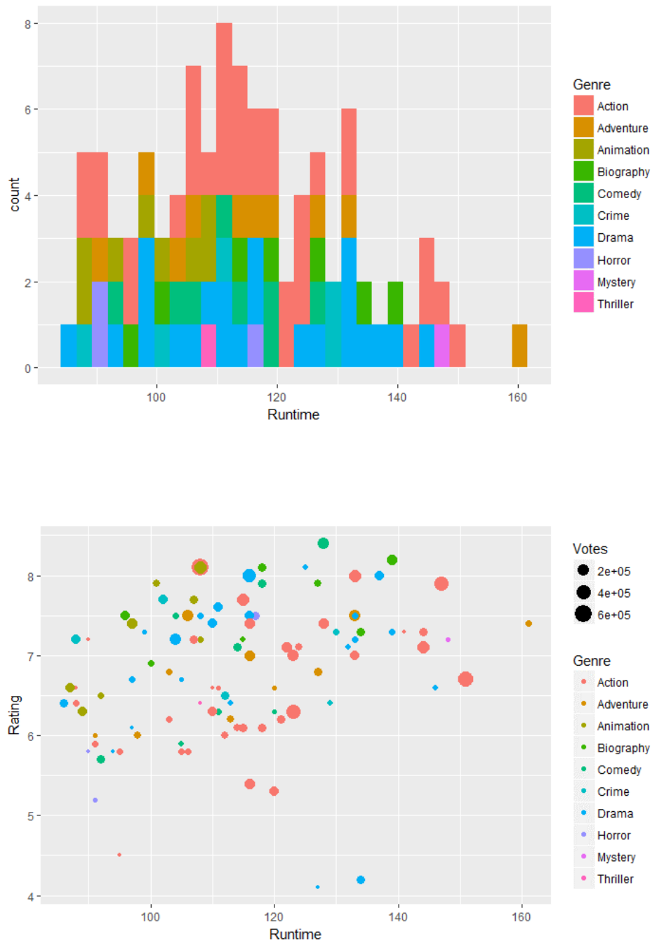
Question 1: Based on the above data, which movie from which Genre had the longest runtime?

ggplot(movies_df,aes(x=Runtime,y=Rating))+

geom_point(aes(size=Votes,col=Genre))

Question 2: Based on the above data, in the Runtime of 130-160 mins, which genre has the highest votes?

ggplot(movies_df,aes(x=Runtime,y=Gross_Earning_in_Mil))+

geom_point(aes(size=Rating,col=Genre))

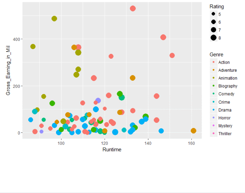
Question 3: Based on the above data, across all genres which genre has the highest average gross earnings in

runtime 100 to 120.

End Notes

I believe this article would have given you a complete understanding of the web scrapping in R. Now, you also

have a fair idea of the problems which you might come across and how you can make your way around them.

As most of the data on theweb is present in an unstructured format, web scrapping is a really handy skill for

any data scientist.