Scientific Computing Python 3
User Manual: scientific-computing-python-3
Open the PDF directly: View PDF ![]() .
.
Page Count: 322 [warning: Documents this large are best viewed by clicking the View PDF Link!]
- Cover
- Copyright
- Credits
- About the Authors
- About the Reviewer
- www.PacktPub.com
- Acknowledgement
- Table of Contents
- Preface
- Chapter 1: Getting Started
- Chapter 2: Variables and Basic Types
- Chapter 3: Container Types
- Chapter 4: Linear Algebra – Arrays
- Chapter 5: Advanced Array Concepts
- Chapter 6: Plotting
- Chapter 7: Functions
- Chapter 8: Classes
- Chapter 9: Iterating
- Chapter 10: Error Handling
- Chapter 11: Namespaces, Scopes, and Modules
- Chapter 12: Input and Output
- Chapter 13: Testing
- Chapter 14: Comprehensive Examples
- Chapter 15: Symbolic Computations - SymPy
- Appendix: References
- Index

Scientific Computing with
Python 3
An example-rich, comprehensive guide for all of your Python
computational needs
Claus Führer
Jan Erik Solem
Olivier Verdier
BIRMINGHAM - MUMBAI
Scientific Computing with Python 3
Copyright © 2016 Packt Publishing
All rights reserved. No part of this book may be reproduced, stored in a retrieval system, or
transmitted in any form or by any means, without the prior written permission of the
publisher, except in the case of brief quotations embedded in critical articles or reviews.
Every effort has been made in the preparation of this book to ensure the accuracy of the
information presented. However, the information contained in this book is sold without
warranty, either express or implied. Neither the authors, nor Packt Publishing, and its
dealers and distributors will be held liable for any damages caused or alleged to be caused
directly or indirectly by this book.
Packt Publishing has endeavored to provide trademark information about all of the
companies and products mentioned in this book by the appropriate use of capitals.
However, Packt Publishing cannot guarantee the accuracy of this information.
First published: December 2016
Production reference: 1141216
Published by Packt Publishing Ltd.
Livery Place
35 Livery Street
Birmingham
B3 2PB, UK.
ISBN 978-1-78646-351-7
www.packtpub.com
Credits
Authors
Claus Führer
Jan Erik Solem
Olivier Verdier
Copy Editor
Vikrant Phadkay
Sneha Singh
Reviewers
Helmut Podhaisky
Project Coordinator
Nidhi Joshi
Commissioning Editor
Veena Pagare
Proofreader
Safis Editing
Acquisition Editor
Sonali Vernekar
Indexer
Mariammal Chettiyar
Content Development Editor
Aishwarya Pandere
Graphics
Disha Haria
Technical Editor
Karan Thakkar
Production Coordinator
Arvindkumar Gupta
About the Authors
Claus Führer is a professor of scientific computations at Lund University, Sweden. He has
an extensive teaching record that includes intensive programming courses in numerical
analysis and engineering mathematics across various levels in many different countries and
teaching environments. Claus also develops numerical software in research collaboration
with industry and received Lund University’s Faculty of Engineering Best Teacher Award
in 2016.
Jan Erik Solem is a Python enthusiast, former associate professor, and currently the CEO of
Mapillary, a street imagery computer vision company. He has previously worked as a face
recognition expert, founder and CTO of Polar Rose, and computer vision team leader at
Apple. Jan is a World Economic Forum technology pioneer and won the Best Nordic Thesis
Award 2005-2006 for his dissertation on image analysis and pattern recognition. He is also
the author of "Programming Computer Vision with Python" (O'Reilly 2012).
Olivier Verdier began using Python for scientific computing back in 2007 and received a
PhD in mathematics from Lund University in 2009. He has held post-doctoral positions in
Cologne, Trondheim, Bergen, and Umeå and is now an associate professor of mathematics
at Bergen University College, Norway.
About the Reviewer
Helmut Podhaisky works in the Institute of Mathematics at the Martin Luther University in
Halle-Wittenberg, where he teaches mathematics and scientific computing. He has co-
authored a book on numerical methods for ordinary differential equations as well as several
research papers on numerical methods. For work and fun, he uses Python, Fortran, Octave,
Mathematica, and Haskell.
www.PacktPub.com
For support files and downloads related to your book, please visit www.PacktPub.com.
Did you know that Packt offers eBook versions of every book published, with PDF and
ePub files available? You can upgrade to the eBook version at www.PacktPub.com and as a
print book customer, you are entitled to a discount on the eBook copy. Get in touch with us
at service@packtpub.com for more details.
At www.PacktPub.com, you can also read a collection of free technical articles, sign up for a
range of free newsletters and receive exclusive discounts and offers on Packt books and
eBooks.
h t t p s ://w w w . p a c k t p u b . c o m /m a p t
Get the most in-demand software skills with Mapt. Mapt gives you full access to all Packt
books and video courses, as well as industry-leading tools to help you plan your personal
development and advance your career.
Why subscribe?
Fully searchable across every book published by Packt
Copy and paste, print, and bookmark content
On demand and accessible via a web browser
Acknowledgement
We want to acknowledge the competent and helpful comments and suggestions by Helmut
Podhaisky, Halle University, Germany. To have such a partner in the process of writing a
book is a big luck and chance for the authors.
We would also like to express our gratitude towards the reviewers of the first edition of this
book, [7], Linda Kann, KTH Stockholm, Hans Petter Langtangen, Simula Research
Laboratory, and Alf Inge Wang, NTNU Trondheim.
A book has to be tested in teaching. And here we had fantastic partners: the teaching
assistants from the course "Beräkningsprogramering med Python" during the years and the
colleagues involved in teaching: Najmeh Abiri, Christian Andersson, Dara Maghdid, Peter
Meisrimel, Fatemeh Mohammadi, Azahar Monge, Anna-Maria Persson, Alexandros
Sopasakis, Tony Stillfjord, Lund University. Najmeh Abiri also tested most of the Jupyter
notebook material which you find on the book's webpage.
A book has not only to be written, it has to be published, and in this process Aishwarya
Pandere and Karan Thakkar, PACKT Publishing, were always constructive, friendly and
helpful partners bridging different time zones and different text processing tools. Thanks.
Claus Führer, Jan-Erik Solem, Olivier Verdier Lund, Bergen 2016

Table of Contents
Preface 1
Chapter 1: Getting Started 10
Installation and configuration instructions 11
Installation 11
Anaconda 12
Configuration 13
Python Shell 13
Executing scripts 14
Getting Help 14
Jupyter – Python notebook 14
Program and program flow 15
Comments 16
Line joining 16
Basic types 17
Numbers 17
Strings 17
Variables 18
Lists 18
Operations on lists 19
Boolean expressions 19
Repeating statements with loops 20
Repeating a task 20
Break and else 21
Conditional statements 21
Encapsulating code with functions 22
Scripts and modules 23
Simple modules – collecting functions 23
Using modules and namespaces 24
Interpreter 24
Summary 25
Chapter 2: Variables and Basic Types 26
Variables 26
Numeric types 27
Integers 28
[ ii ]
Plain integers 28
Floating point numbers 29
Floating point representation 29
Infinite and not a number 30
Underflow – Machine Epsilon 31
Other float types in NumPy 32
Complex numbers 33
Complex Numbers in Mathematics 33
The j notation 33
Real and imaginary parts 34
Booleans 36
Boolean operators 36
Boolean casting 37
Automatic Boolean casting 38
Return values of and and or 38
Boolean and integer 39
Strings 39
Operations on strings and string methods 41
String formatting 42
Summary 43
Exercises 43
Chapter 3: Container Types 47
Lists 47
Slicing 48
Strides 50
Altering lists 51
Belonging to a list 51
List methods 52
In–place operations 52
Merging lists – zip 53
List comprehension 53
Arrays 54
Tuples 56
Dictionaries 56
Creating and altering dictionaries 57
Looping over dictionaries 58
Sets 58
Container conversions 60
Type checking 61
Summary 62

[ iii ]
Exercises 62
Chapter 4: Linear Algebra – Arrays 65
Overview of the array type 65
Vectors and matrices 65
Indexing and slices 67
Linear algebra operations 67
Solving a linear system 68
Mathematical preliminaries 69
Arrays as functions 69
Operations are elementwise 69
Shape and number of dimensions 70
The dot operations 71
The array type 73
Array properties 73
Creating arrays from lists 74
Accessing array entries 75
Basic array slicing 75
Altering an array using slices 77
Functions to construct arrays 77
Accessing and changing the shape 78
The shape function 78
Number of dimensions 79
Reshape 79
Transpose 81
Stacking 82
Stacking vectors 82
Functions acting on arrays 83
Universal functions 83
Built-in universal functions 83
Create universal functions 84
Array functions 86
Linear algebra methods in SciPy 87
Solving several linear equation systems with LU 87
Solving a least square problem with SVD 89
More methods 90
Summary 91
Exercises 91
Chapter 5: Advanced Array Concepts 94
Array views and copies 94
Array views 94

[ iv ]
Slices as views 95
Transpose and reshape as views 95
Array copy 96
Comparing arrays 96
Boolean arrays 96
Checking for equality 97
Boolean operations on arrays 98
Array indexing 99
Indexing with Boolean arrays 99
Using where 100
Performance and Vectorization 101
Vectorization 102
Broadcasting 103
Mathematical view 103
Constant functions 104
Functions of several variables 105
General mechanism 105
Conventions 107
Broadcasting arrays 107
The broadcasting problem 107
Shape mismatch 109
Typical examples 110
Rescale rows 110
Rescale columns 110
Functions of two variables 110
Sparse matrices 112
Sparse matrix formats 113
Compressed sparse row 113
Compressed Sparse Column 115
Row-based linked list format 115
Altering and slicing matrices in LIL format 116
Generating sparse matrices 116
Sparse matrix methods 117
Summary 118
Chapter 6: Plotting 119
Basic plotting 119
Formatting 125
Meshgrid and contours 128
Images and contours 132
Matplotlib objects 134
The axes object 135
[ v ]
Modifying line properties 136
Annotations 137
Filling areas between curves 138
Ticks and ticklabels 140
Making 3D plots 141
Making movies from plots 145
Summary 146
Exercises 147
Chapter 7: Functions 149
Basics 149
Parameters and arguments 150
Passing arguments – by position and by keyword 150
Changing arguments 151
Access to variables defined outside the local namespace 152
Default arguments 153
Beware of mutable default arguments 154
Variable number of arguments 154
Return values 156
Recursive functions 157
Function documentation 159
Functions are objects 160
Partial application 160
Using Closures 161
Anonymous functions – the lambda keyword 161
The lambda construction is always replaceable 162
Functions as decorators 163
Summary 164
Exercises 165
Chapter 8: Classes 167
Introduction to classes 168
Class syntax 169
The __init__ method 169
Attributes and methods 170
Special methods 172
Reverse operations 174
Attributes that depend on each other 176
The property function 177
Bound and unbound methods 178
Class attributes 178

[ vi ]
Class methods 179
Subclassing and inheritance 181
Encapsulation 184
Classes as decorators 185
Summary 188
Exercises 188
Chapter 9: Iterating 190
The for statement 190
Controlling the flow inside the loop 191
Iterators 192
Generators 193
Iterators are disposable 194
Iterator tools 194
Generators of recursive sequences 196
Arithmetic geometric mean 196
Convergence acceleration 198
List filling patterns 200
List filling with the append method 200
List from iterators 200
Storing generated values 201
When iterators behave as lists 202
Generator expression 202
Zipping iterators 203
Iterator objects 204
Infinite iterations 205
The while loop 205
Recursion 206
Summary 207
Exercises 207
Chapter 10: Error Handling 210
What are exceptions? 210
Basic principles 212
Raising exceptions 212
Catching exceptions 213
User-defined exceptions 215
Context managers — the with statement 216
Finding Errors: Debugging 218
Bugs 218
The stack 218

[ vii ]
The Python debugger 219
Overview – debug commands 221
Debugging in IPython 222
Summary 223
Chapter 11: Namespaces, Scopes, and Modules 224
Namespace 224
Scope of a variable 225
Modules 227
Introduction 227
Modules in IPython 229
The IPython magic command 229
The variable __name__ 229
Some useful modules 230
Summary 230
Chapter 12: Input and Output 231
File handling 231
Interacting with files 231
Files are iterable 233
File modes 233
NumPy methods 234
savetxt 234
loadtxt 234
Pickling 235
Shelves 236
Reading and writing Matlab data files 237
Reading and writing images 237
Summary 238
Chapter 13: Testing 239
Manual testing 239
Automatic testing 240
Testing the bisection algorithm 241
Using unittest package 243
Test setUp and tearDown methods 244
Parameterizing tests 245
Assertion tools 247
Float comparisons 247
Unit and functional tests 249
Debugging 250

[ viii ]
Test discovery 250
Measuring execution time 250
Timing with a magic function 251
Timing with the Python module timeit 252
Timing with a context manager 253
Summary 254
Exercises 254
Chapter 14: Comprehensive Examples 256
Polynomials 256
Theoretical background 256
Tasks 258
The polynomial class 259
Newton polynomial 263
Spectral clustering 265
Solving initial value problems 269
Summary 273
Exercises 273
Chapter 15: Symbolic Computations - SymPy 274
What are symbolic computations? 274
Elaborating an example in SymPy 276
Basic elements of SymPy 278
Symbols – the basis of all formulas 278
Numbers 279
Functions 279
Undefined functions 280
Elementary Functions 281
Lambda – functions 282
Symbolic Linear Algebra 283
Symbolic matrices 284
Examples for Linear Algebra Methods in SymPy 285
Substitutions 287
Evaluating symbolic expressions 289
Example: A study on the convergence order of Newton's Method 290
Converting a symbolic expression into a numeric function 292
A study on the parameter dependency of polynomial coefficients 292
Summary 294
Appendix: References 295
Index 298
Preface
Python can be used for more than just general-purpose programming. It is a free, open
source language and environment that has tremendous potential for use within the domain
of scientific computing. This book presents Python in tight connection with mathematical
applications and demonstrates how to use various concepts in Python for computing
purposes, including examples with the latest version of Python 3. Python is an effective tool
to use when coupling scientific computing and mathematics and this book will teach you
how to use it for linear algebra, arrays, plotting, iterating, functions, polynomials, and much
more.
What this book covers
Chapter 1, Getting Started, addresses the main language elements of Python without going
into detail. Here we make a brief tour through all. It is a good starting point for those who
want to start directly. It is a quick reference for those readers who want in a later chapter
understand an example which uses might use constructs like functions before functions
were explained in deep .
Chapter 2, Variables and Basic Types, presents the most important and basic types in Python.
Float is the more important datatype in scientific computing together with the special
numbers nan and inf. Booleans, integers, complex, and strings are other basic datatypes,
which will be used throughout this book.
Chapter 3, Container Types, explains how to work with container types, mainly lists.
Dictionaries and tuples will be explained as well as indexing and looping, through
container objects. Occasionally, one uses even sets as a special container type.
Chapter 4, Linear Algebra, works with the most important objects in linear algebra--vectors
and matrices. This book chooses NumPy array as the central tool for describing matrices
and even higher order tensors. Arrays have many advanced features and allows also for
universal functions acting on matrices or vectors elementwise. The book emphasizes on
array indexing, slices, and the dot product as the basic operation in most computing tasks.
Some linear algebra examples are worked out to demonstrate the use of SciPy's submodule
linalg.

Preface
[ 2 ]
Chapter 5, Advanced Array Concepts, explains some more advanced aspects of arrays. The
difference between array copies and views is explained extensively as views make
programs using arrays very fast but are often a source for errors, which are hard to debug.
The use of Boolean arrays to write effective, compact, and readable code is shown and
demonstrated. Finally, the technique of array broadcasting-- a unique feature of NumPy
arrays -- is explained by its analogy to operations performed on functions.
Chapter 6, Plotting, shows how to make plots, mainly classical x/yplots but also 3D plots
and histograms. Scientific computing requires good tools for visualizing the results.
Python's module matplotlib is introduced starting from the handy plotting commands in its
submodule pyplot. Finetuning and modifying plots becomes possible by creating graphical
objects such as axes. We show how attributes of these objects can be changed and
annotations can be made.
Chapter 7, Functions, form the fundamental building block in programming, which is
probably nearest to underlying mathematical concepts. Function definition and function
calls are explained as the different ways to set function arguments. Anonymous lambda
functions are introduced and used in various examples throughout the book.
Chapter 8, Classes, defines objects as instances of classes, which we provide with methods
and attributes. In mathematics, class attributes often depend on each other, which requires
special programming techniques for setter and getter functions. Basic mathematical
operations such as + can be defined for special mathematic datatypes. Inheritance and
abstraction are mathematical concepts which are reflected by object oriented programming.
We demonstrate the use of inheritance by a simple solver class for ordinary differential
equations.
Chapter 9, Iterating, presents iteration using loops and iterators. There is now a chapter in
this book without loops and iterations, but here we come to principles of iterators and
create own generator objects. In this chapter, you learn why a generator can be exhausted
and how infinite loops can be programmed. Python's module itertools is a useful
companion for this chapter.
Chapter 10, Error Handling, covers errors and exceptions and how to find and fix them. An
error or an exception is an event, which breaks the execution of a program unit. This
chapter shows what to do then, that is, how an exception can be handled. You learn to
define your own exception classes and how to provide valuable information, which can be
used for catching these exceptions. Error handling is more than printing an error message.

Preface
[ 3 ]
Chapter 11, Namespaces, Scopes and Modules, covers Python modules. What are local and
global variables? When is a variable known and when is it unknown to a program unit?
This is discussed in this chapter. A variable can be passed to a function by a parameter list
or tacitly injected by making use of its scope. When should this technique be applied and
when not? This chapter tries to give an answer to this central question.
Chapter 12, Input and Output, covers some options for handling data files. Data files are
used for storing and providing data for a given problem, often large scale measurements.
This chapter describes how this data can be accessed and modified using different formats.
Chapter 13, Testing, focuses on testing for scientific programming. The key tool is unittest,
which allows for automatic testing and parametrized tests. By considering the classical
bisection algorithm in numerical mathematics, we exemplify different steps to design
meaningful tests, which as a side effect also deliver a documentation of the use of a piece of
code. Careful testing provides test protocols which can be later helpful when debugging a
complex code often written by many different programmers.
Chapter 14, Comprehensive Examples, presents some comprehensive and longer examples
together with a brief introduction to the theoretical background and their complete
implementation. These examples make use of all constructs shown in the book so far and
put them in a larger and more complex context. They are open for extensions by the reader.
Chapter 15, Symbolic Computations - SymPy, speaks about symbolic computations. Scientific
computing is mainly numeric computations with inexact data and approximative results.
This is contrasted by symbolic computations often formal manipulation, which aims for
exact solutions in a closed form expression. In this last chapter of the book, we introduce
this technique in Python, which is often used for deriving and verifying theoretically
mathematical models and numerical results. We emphasize on high precision floating point
evaluation of symbolic expressions.
What you need for this book
You would need Pyhon3.5 or higher, SciPy, NumPy, Matplotlib, IPython shell (we
recommend strongly to install Python and its packages through Anaconda). The examples
of the book do not have any special hardware requirements on memory and graphics.

Preface
[ 4 ]
Who this book is for
This book is the outcome of a course on Python for scientific computing which is taught at
Lund University since 2008. The course expanded over the years, and condensed versions
of the material were taught at universities in Cologne, Trondheim, Stavanger, Soran,
Lappeenranta and also in computation oriented companies.
Our belief is that Python and its surrounding scientific computing ecosystem — SciPy,
NumPY and matplotlib — represent a tremendous progress in scientific computing
environment. Python and the aforementioned libraries are free and open source. What’s
more, is a modern language featuring all the bells and whistles that this adjective entails:
object oriented programming, testing, advanced shell with IPython, etc. When writing this
book we had two groups of readers in mind:
The reader who chooses Python as his or her first programming language will
use this book in a teacher-led course. The book guides into the different topics
and offers background reading and experimenting. A teacher typically selects
and orders the material from this book in such a way, that it fits to the specific
learning outcomes of an introductory course.
The reader who already has some experience in programming, and some taste for
scientific computing or mathematics will use this book as a companion when
diving into the world of Scipy and Numpy. Programming in Python can be quite
different from programming in MATLAB, say. The book wants to point out the
"pythonic" way of programming, which makes programming a pleasure.
Our goal is to explain the steps to get started with Python in the context of scientific
computing. The book may be read either from the first page to the last, or by picking the
bits that seem most interesting. Needless to say, as improving one’s programming skills
requires considerable practice, it is highly advisable to experiment and play with the
examples and the exercises in the book.
We hope that the readers will enjoy programming with Python, SciPy, NumPY and
matplotlib as much as we do.
Preface
[ 5 ]
Python vs Other Languages
When it comes to deciding what language to use for a book on scientific computing many
factors come in to play. The learning threshold of the language itself is important for
newcomers, here scripting languages usually provide the best options. A wide range of
modules for numerical computing is necessary, preferably with a strong developer
community. If these core modules are built on a well-tested, optimized foundation of fast
libraries like e.g. LAPACK, even better. Finally, if the language is also usable in a wider
setting and a wider range of applications, the chance of the reader using the skills learned
from this book outside an academic setting is greater. Therefore the choice of Python was a
natural one.
In short, Python is
free and open source
a scripting language, meaning that it is interpreted
a modern language (object oriented, exception handling, dynamic typing etc.)
concise, easy to read and quick to learn
full of freely available libraries, in particular scientific ones (linear algebra,
visualization tools, plotting, image analysis, differential equations solving,
symbolic computations, statistics etc.)
useful in a wider setting: scientific computing, scripting, web sites, text parsing,
etc.
widely used in industrial applications
There are other alternatives to Python. Some of them and the differences to Python are
listed here.
Java, C++ : Object oriented, compiled languages. More verbose and low level compared to
Python. Few scientific libraries.
C, FORTRAN : Low level compiled languages. Both languages are extensively used in
scientific computing, where computational time matters. Nowadays these languages are
often combined with Python wrappers.
PHP, Ruby, other interpreted languages. PHP is web oriented. Ruby is as flexible as Python
but has few scientific libraries.

Preface
[ 6 ]
MATLAB, Scilab, Octave : MATLAB is a tool for matrix computation that evolved for
scientific computing. The scientific library is huge. The language features are not as
developed as those of Python. Neither free nor open source. SciLab and Octave are open
source tools which are syntactically similar to MATLAB.
Haskell : Haskell is a modern functional language and follows different programming
paradigms than Python. There are some common constructions like list comprehension.
Haskell is rarely used in scientific computing. See also [12].
Other Python literature
Here we give some hints to literature on Python which can serve as complementary sources
or as texts for parallel reading. Most introductory books on Python are devoted to teach this
language as a general purpose tool. One excellent example which we want to mention here
explicitly is [19]. It explains the language by simple examples, e.g. object oriented
programming is explained by organizing a pizza bakery.
There are very few books dedicated to Python directed towards scientific computing and
engineering. Among these few books we would like to mention the two books by
Langtangen which combine scientific computing with the modern "pythonic" view on
programming, [16,17].
This "pythonic" view is also the guiding line of our way of teaching programming of
numerical algorithms. We try to show how many well-established concepts and
constructions in computer science can be applied to problems within scientific computing.
The pizza-bakery example is replaced by Lagrange polynomials, generators become time
stepping methods for ODEs, and so on.
Finally we have to mention the nearly infinite amount of literature on the web. The web
was also a big source of knowledge when preparing this book. Literature from the web
often covers things that are new, but can also be totally outdated. The web also presents
solutions and interpretations which might contradict each other. We strongly recommend
to use the web as additional source, but we consider a "traditional" textbook with the web
resources "edited" as the better entry point to a rich new world.

Preface
[ 7 ]
Conventions
In this book, you will find a number of text styles that distinguish between different kinds
of information. Here are some examples of these styles and an explanation of their meaning.
Code words in text, database table names, folder names, filenames, file extensions,
pathnames, and user input are shown as follows: "install additional packages with conda
install within your virtual environment"
A block of code is set as follows:
from scipy import *
from matplotlib.pyplot import *
Any command-line input or output is written as follows:
jupyter notebook
New terms and important words are shown in bold. Words that you see on the screen, for
example, in menus or dialog boxes, appear in the text like this: "The Jupyter notebook is a
fantastic tool for demonstrating your work."
Warnings or important notes appear in a box like this.
Tips and tricks appear like this.
Reader feedback
Feedback from our readers is always welcome. Let us know what you think about this
book-what you liked or disliked. Reader feedback is important for us as it helps us develop
titles that you will really get the most out of. To send us general feedback, simply e-
mail feedback@packtpub.com, and mention the book's title in the subject of your
message. If there is a topic that you have expertise in and you are interested in either
writing or contributing to a book, see our author guide at www.packtpub.com/authors.
Preface
[ 8 ]
Customer support
Now that you are the proud owner of a Packt book, we have a number of things to help you
to get the most from your purchase.
Downloading the example code
You can download the example code files for this book from your account at h t t p ://w w w . p
a c k t p u b . c o m . If you purchased this book elsewhere, you can visit h t t p ://w w w . p a c k t p u b . c
o m /s u p p o r t and register to have the files e-mailed directly to you.
You can download the code files by following these steps:
Log in or register to our website using your e-mail address and password.1.
Hover the mouse pointer on the SUPPORT tab at the top.2.
Click on Code Downloads & Errata.3.
Enter the name of the book in the Search box.4.
Select the book for which you're looking to download the code files.5.
Choose from the drop-down menu where you purchased this book from.6.
Click on Code Download.7.
Once the file is downloaded, please make sure that you unzip or extract the folder using the
latest version of:
WinRAR / 7-Zip for Windows
Zipeg / iZip / UnRarX for Mac
7-Zip / PeaZip for Linux
The code bundle for the book is also hosted on GitHub at h t t p s ://g i t h u b . c o m /P a c k t P u b l
i s h i n g /S c i e n t i f i c - C o m p u t i n g - w i t h - P y t h o n - 3. We also have other code bundles from
our rich catalog of books and videos available at h t t p s ://g i t h u b . c o m /P a c k t P u b l i s h i n g /.
Check them out!
Downloading the color images of this book
We also provide you with a PDF file that has color images of the screenshots/diagrams used
in this book. The color images will help you better understand the changes in the output.
You can download this file from h t t p s ://w w w . p a c k t p u b . c o m /s i t e s /d e f a u l t /f i l e s /d o w n
l o a d s /S c i e n t i f i c C o m p u t i n g w i t h P y t h o n 3_ C o l o r I m a g e s . p d f .

Preface
[ 9 ]
Errata
Although we have taken every care to ensure the accuracy of our content, mistakes do
happen. If you find a mistake in one of our books-maybe a mistake in the text or the code-
we would be grateful if you could report this to us. By doing so, you can save other readers
from frustration and help us improve subsequent versions of this book. If you find any
errata, please report them by visiting h t t p ://w w w . p a c k t p u b . c o m /s u b m i t - e r r a t a , selecting
your book, clicking on the Errata Submission Form link, and entering the details of your
errata. Once your errata are verified, your submission will be accepted and the errata will
be uploaded to our website or added to any list of existing errata under the Errata section of
that title.
To view the previously submitted errata, go to h t t p s ://w w w . p a c k t p u b . c o m /b o o k s /c o n t e n
t /s u p p o r t and enter the name of the book in the search field. The required information will
appear under the Errata section.
Piracy
Piracy of copyrighted material on the Internet is an ongoing problem across all media. At
Packt, we take the protection of our copyright and licenses very seriously. If you come
across any illegal copies of our works in any form on the Internet, please provide us with
the location address or website name immediately so that we can pursue a remedy.
Please contact us at copyright@packtpub.com with a link to the suspected pirated
material.
We appreciate your help in protecting our authors and our ability to bring you valuable
content.
Questions
If you have a problem with any aspect of this book, you can contact us
at questions@packtpub.com, and we will do our best to address the problem.
1
Getting Started
In this chapter, we will give a brief overview of the principal syntactical elements of Python.
Readers who have just started learning programming are guided through the book in this
chapter. Every topic is presented here in a how-to way and will be explained later in the
book in a deeper conceptual manner and will also be enriched with many applications and
extensions.
Readers who are already familiar with another programming language will come across, in
this chapter, the Python way of doing classical language constructs. It offers them a quick
start to Python programming.
Both types of readers are encouraged to take this chapter as a brief guideline when
zigzagging through the book. However, before we start we have to make sure that
everything is in place and you have the correct version of Python installed together with the
main modules for Scientific Computing and tools, such as a good editor and a shell, which
helps in code developing and testing.
Read the following section, even if you already have access to a computer with Python
installed. You might want to adjust things to have a working environment conforming to
the presentation in this book.

Getting Started
[ 11 ]
Installation and configuration instructions
Before diving into the subject of the book you should have all the relevant tools installed on
your computer. We will give you some advice and recommend tools that you might want to
use. We only describe public domain and free tools.
Installation
There are currently two major versions of Python; the 2.x branch and the new 3.x branch.
There are language incompatibilities between these branches and one has to be aware of
which one to use. This book is based on the 3.x branch, considering the language up to
release 3.5.
For this book you need to install the following:
The interpreter: Python 3.5 (or later)
The modules for scientific computing: SciPy with NumPy
The module for graphical representation of mathematical results: matplotlib
The shell: IPython
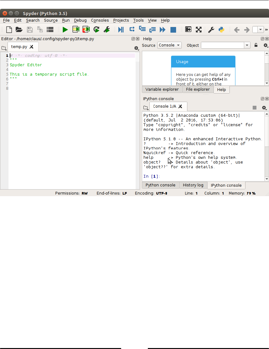
A Python related editor: Spyder (refer to the following Figure 1.1, Spyder), Geany
The installation of these is eased by the so-called distribution packages. We recommend that
you use Anaconda. The default screen of Spyder consists of an editor window on left, a
console window in the lower right corner which gives access to an IPython shell and a help
window in the upper right corner as shown in the following figure:
Getting Started
[ 12 ]
Figure 1.1: The default screen of Spyder consists of an editor window on left, a
console window in the lower right corner which gives access to an IPython shell
and a help window in the upper right corner.
Anaconda
Even if you have Python pre-installed on your computer, we recommend that you create
your personal Python environment that allows you to work without the risk of accidentally
affecting the software on which your computer's functionality might depend. With a virtual
environment, such as Anaconda, you are free to change language versions and install
packages without the unintended side-effects.
If the worst happens and you screw things up totally, just delete the Anaconda directory
and start again. Running the Anaconda installer will install Python, a Python development
environment and editor (Spyder), the shell IPython, and the most important packages for
numerical computations, for example SciPy, NumPy, and matplotlib.
Getting Started
[ 13 ]
You can install additional packages with conda install within your virtual environment
created by Anaconda (refer for official documentation from[2]) .
Configuration
Most Python codes will be collected in files. We recommend that you use the following
header in all your Python files:
from scipy import *
from matplotlib.pyplot import *
With this, you make sure that all standard modules and functions used in this book, such as
SciPy, are imported. Without this step, most of the examples in the book would raise errors.
Many editors, such as Spyder, provide the possibility to create a template for your files.
Look for this feature and put the preceding header into a template.
Python Shell
The Python shell is good but not optimal for interactive scripting. We therefore recommend
using IPython instead (refer to [26] for the official documentation). IPython can be started
in different ways:
In a terminal shell by running the following command: ipython
By directly clicking on an icon called Jupyter QT Console
When working with Spyder you should use an IPython console (refer to Figure
1.1, Spyder).

Getting Started
[ 14 ]
Executing scripts
You often want to execute the contents of a file. Depending on the location of the file on
your computer, it is necessary to navigate to the correct location before executing the
contents of a file.
Use the command cd in IPython in order to move to the directory where your file
is located.
To execute the contents of a file named myfile.py, just run the following
command in the IPython shell
run myfile
Getting Help
Here are some tips on how to use IPython:
To get help on an object, just type ? after the object's name and then return.
Use the arrow keys to reuse the last executed commands.
You may use the Tab key for completion (that is, you write the first letter of a
variable or method and IPython shows you a menu with all the possible
completions).
Use Ctrl+D to quit.
Use IPython's magic functions. You can find a list and explanations by applying
%magic on the command prompt.
You can find out more about IPython in its online documentation, [15].
Jupyter – Python notebook
The Jupyter notebook is a fantastic tool for demonstrating your work. Students might want
to use it to make and document homework and exercises and teachers can prepare lectures
with it, even slides and web pages.
Getting Started
[ 15 ]
If you have installed Python via Anaconda, you already have everything for Jupyter in
place. You can invoke the notebook by running the following command in the terminal
window:
jupyter notebook
A browser window will open and you can interact with Python through your web browser.
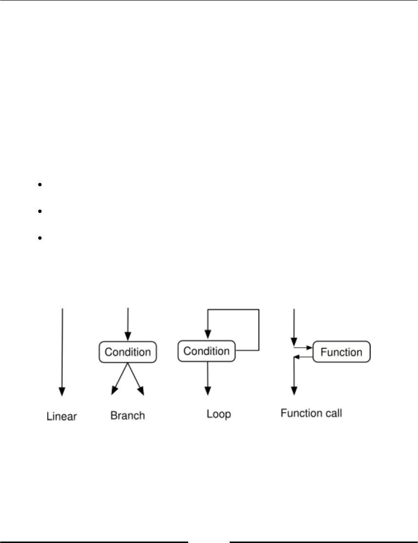
Program and program flow
A program is a sequence of statements that are executed in a top-down order. This linear
execution order has some important exceptions:
There might be a conditional execution of alternative groups of statements
(blocks), which we refer to as branching.
There are blocks that are executed repetitively, which is
called looping (refer to the following Figure 1.2, Program flow).
There are function calls that are references to another piece of code, which is
executed before the main program flow is resumed. A function call breaks the
linear execution and pauses the execution of a program unit while it passes the
control to another unit–a function. When this gets completed, its control is
returned to the calling unit.
Figure 1.2: Program flow
Getting Started
[ 16 ]
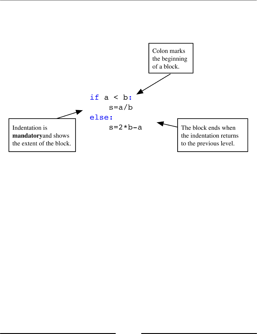
Python uses a special syntax to mark blocks of statements: a keyword, a colon, and an
indented sequence of statements, which belong to the block (refer to the following Figure
1.3, Block command).
Figure 1.3: Block command
Comments
If a line in a program contains the symbol #, everything following on the same line is
considered as a comment:
# This is a comment of the following statement
a = 3 # ... which might get a further comment here
Line joining
A backslash \ at the end of the line marks the next line as a continuation line, that is, explicit
line joining. If the line ends before all the parentheses are closed, the following line will
automatically be recognized as a continuation line, that is, implicit line joining.
Getting Started
[ 17 ]
Basic types
Let's go over the basic data types that you will encounter in Python.
Numbers
A number may be an integer, a real number, or a complex number. The usual operations
are:
addition and subtraction, + and -
multiplication and division, * and /
power, **
Here is an example:
2 ** (2 + 2) # 16
1j ** 2 # -1
1. + 3.0j
The symbol for complex numbers
j is a symbol to denote the imaginary part of a complex number.
It is a syntactic element and should not be confused with multiplication by
a variable. More on complex numbers can be found in section Numeric
Types of Chapter 2, Variables and Basic Types.
Strings
Strings are sequences of characters, enclosed by simple or double quotes:
'valid string'
"string with double quotes"
"you shouldn't forget comments"
'these are double quotes: ".." '
You can also use triple quotes for strings that have multiple lines:
"""This is
a long,
long string"""

Getting Started
[ 18 ]
Variables
A variable is a reference to an object. An object may have several references. One uses the
assignment operator = to assign a value to a variable:
x = [3, 4] # a list object is created
y = x # this object now has two labels: x and y
del x # we delete one of the labels
del y # both labels are removed: the object is deleted
The value of a variable can be displayed by the print function:
x = [3, 4] # a list object is created
print(x)
Lists
Lists are a very useful construction and one of the basic types in Python. A Python list is an
ordered list of objects enclosed by square brackets. One can access the elements of a list
using zero-based indexes inside square brackets:
L1 = [5, 6]
L1[0] # 5
L1[1] # 6
L1[2] # raises IndexError
L2 = ['a', 1, [3, 4]]
L2[0] # 'a'
L2[2][0] # 3
L2[-1] # last element: [3,4]
L2[-2] # second to last: 1
Indexing of the elements starts at zero. One can put objects of any type inside a list, even
other lists. Some basic list functions are as follows:
list(range(n))} creates a list with n elements, starting with zero:
print(list(range(5))) # returns [0, 1, 2, 3, 4]
len gives the length of a list:
len(['a', 1, 2, 34]) # returns 4
Getting Started
[ 19 ]
append is used to append an element to a list:
L = ['a', 'b', 'c']
L[-1] # 'c'
L.append('d')
L # L is now ['a', 'b', 'c', 'd']
L[-1] # 'd'
Operations on lists
The operator + concatenates two lists:
L1 = [1, 2]
L2 = [3, 4]
L = L1 + L2 # [1, 2, 3, 4]
As one might expect, multiplying a list with an integer concatenates the list with
itself several times:
n*L is equivalent to making n additions.
L = [1, 2]
3 * L # [1, 2, 1, 2, 1, 2]
Boolean expressions
A Boolean expression is an expression that may have the value True or False. Some
common operators that yield conditional expressions are as follow:
Equal, ==
Not equal, !=
Less than, Less than or equal to, < , <=
Greater than, Greater than or equal to, > , >=

Getting Started
[ 20 ]
One combines different Boolean values with or and and.
The keyword not , gives the logical negation of the expression that follows. Comparisons
can be chained so that, for example, x < y < z is equivalent to x < y and y < z. The
difference is that y is only evaluated once in the first example.
In both cases, z is not evaluated at all when the first condition, x < y, evaluates to False:
2 >= 4 # False
2 < 3 < 4 # True
2 < 3 and 3 < 2 # False
2 != 3 < 4 or False # True
2 <= 2 and 2 >= 2 # True
not 2 == 3 # True
not False or True and False # True!
Precedence rules
The <, >, <=, >=, !=, and == operators have higher precedence than not.
The operators and, or have the lowest precedence. Operators with higher
precedence rules are evaluated before those with lower.
Repeating statements with loops
Loops are used to repetitively execute a sequence of statements while changing a variable
from iteration to iteration. This variable is called the index variable. It is successively
assigned to the elements of a list, (refer to Chapter 9, Iterating):
L = [1, 2, 10]
for s in L:
print(s * 2) # output: 2 4 20
The part to be repeated in the for loop has to be properly indented:
for elt in my_list:
do_something
something_else
print("loop finished") # outside the for block
Repeating a task
One typical use of a for loop is to repeat a certain task a fixed number of times:
n = 30
for iteration in range(n):
do_something # this gets executed n times
Getting Started
[ 21 ]
Break and else
The for statement has two important keywords: break and else. break quits the for loop
even if the list we are iterating is not exhausted:
for x in x_values:
if x > threshold:
break
print(x)
The finalizing else checks whether the for loop was broken with the break keyword. If it
was not broken, the block following the else keyword is executed:
for x in x_values:
if x > threshold:
break
else:
print("all the x are below the threshold")
Conditional statements
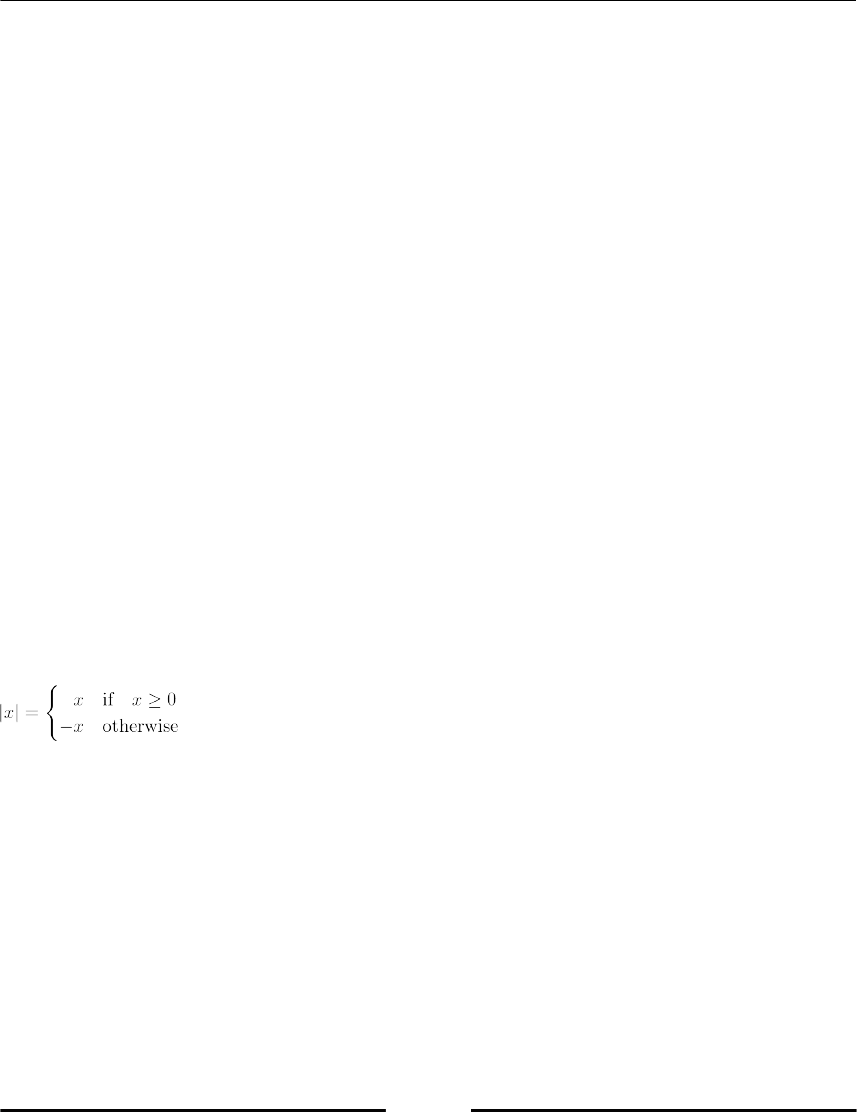
This section covers how to use conditions for branching, breaking, or otherwise controlling
your code. A conditional statement delimits a block that will be executed if the condition is
true. An optional block, started with the keyword else will be executed if the condition is
not fulfilled (refer to Figure 1.3, Block command diagram). We demonstrate this by printing
|x|, the absolute value of x:
The Python equivalent is as follows:
x = ...
if x >= 0:
print(x)
else:
print(-x)
Any object can be tested for the truth value, for use in an if or while statement. The rules
for how the truth values are obtained are explained in section Boolean of Chapter 2,
Variables and Basic Types.
Getting Started
[ 22 ]
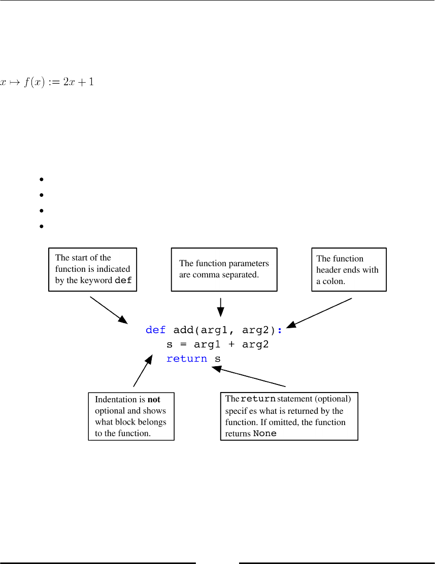
Encapsulating code with functions
Functions are useful for gathering similar pieces of code in one place. Consider the
following mathematical function:
The Python equivalent is as follows:
def f(x):
return 2*x + 1
In Figure 1.4 Anatomy of a function the elements of a function block are explained.
The keyword def tells Python we are defining a function.
f is the name of the function.
x is the argument, or input of the function.
What is after return is called the output of the function.
Figure 1.4: Anatomy of a function
Once the function is defined, it can be called using the following code:
f(2) # 5
f(1) # 3

Getting Started
[ 23 ]
Scripts and modules
A collection of statements in a file (which usually has a py extension), is called a script.
Suppose we put the contents of the following code into a file named smartscript.py:
def f(x):
return 2*x + 1
z = []
for x in range(10):
if f(x) > pi:
z.append(x)
else:
z.append(-1)
print(z)
In a Python or IPython shell, such a script can then be executed with the exec command
after opening and reading the file. Written as a one-liner it reads:
exec(open('smartscript.py').read())
The IPython shell provides the magic command %run as a handy alternative way to execute
a script:
%run smartscript
Simple modules – collecting functions
Often one collects functions in a script. This creates a module with additional Python
functionality. To demonstrate this, we create a module by collecting functions in a single
file, for example smartfunctions.py:
def f(x):
return 2*x + 1
def g(x):
return x**2 + 4*x - 5
def h(x):
return 1/f(x)
These functions can now be used by any external script or directly in the IPython
environment.
Functions within the module can depend on each other.
Grouping functions with a common theme or purpose gives modules that can be
shared and used by others.

Getting Started
[ 24 ]
Again, the command exec(open('smartfunctions.py').read()) makes these
functions available to your IPython shell (note that there is also the IPython magic function
run). In Python terminology, one says that they are put into the actual namespace.
Using modules and namespaces
Alternatively, the modules can be imported by the command import. It creates a
named namespace. The command from puts the functions into the general namespace:
import smartfunctions
print(smartfunctions.f(2)) # 5
from smartfunctions import g #import just this function
print(g(1)) # 0
from smartfunctions import * #import all
print(h(2)*f(2)) # 1.0
Import
The commands import and from import the functions only once into the
respective namespace. Changing the functions after the import has no
effect for the current Python session. More on modules can be found in
section Modules of Chapter 11, Namespaces, Scopes and Modules.
Interpreter
The Python interpreter executes the following steps:
First, run the syntax.
Then execute the code line by line.
Code inside a function or class declaration is not executed (but checked for
syntax).
def f(x):
return y**2
a = 3 # here both a and f are defined

Getting Started
[ 25 ]
You can run the preceding program because there are no syntactical errors. You get an error
only when you call the function f.
f(2) # error, y is not defined
Summary
In this chapter, we briefly addressed the main language elements of Python without going
into detail.
You should now be able to start playing with small pieces of code and to test different
program constructs. All this is intended as an appetizer for the following chapters in which
we will give you the details, examples, exercises, and more background information.
2
Variables and Basic Types
In this chapter, we will present the most important and basic types in Python. What is a
type? It is a set consisting of data content, its representation, and all possible operations.
Later in this book, we will make this definition much more precise, when we introduce the
concepts of a class in Chapter 8, Classes.
Variables
Variables are references to Python objects. They are created by assignments, for example:
a = 1
diameter = 3.
height = 5.
cylinder = [diameter, height] # reference to a list
Variables take names that consist of any combination of capital and small letters, the
underscore _ , and digits. A variable name must not start with a digit. Note that variable
names are case sensitive. A good naming of variables is an essential part of documenting
your work, so we recommend that you use descriptive variable names.
Variables and Basic Types
[ 27 ]
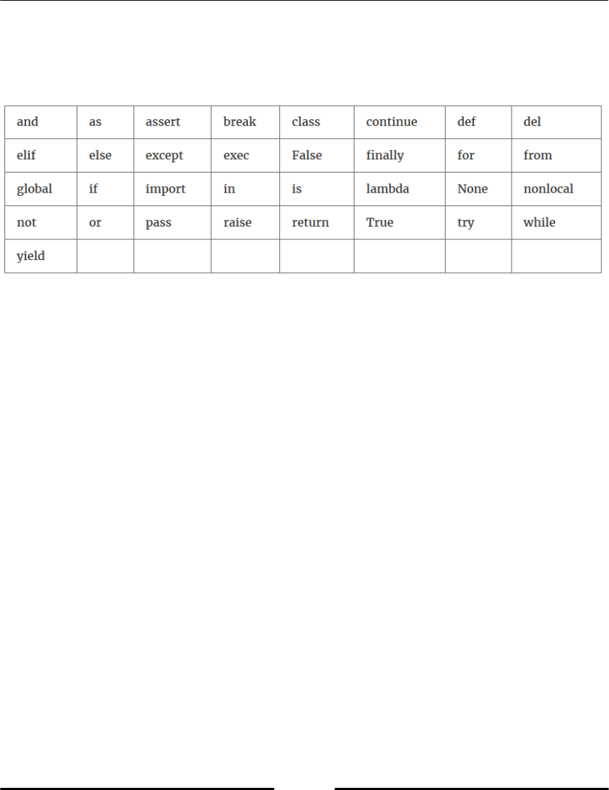
Python has some reserved keywords, which cannot be used as variable names (refer to
following table, Table 2.1). An attempt to use such a keyword as variable name would raise
a syntax error.
Table 2.1: Reserved Python keywords.
As opposed to other programming languages, variables require no type declaration. You
can create several variables with a multiple assignment statement:
a = b = c = 1 # a, b and c get the same value 1
Variables can also be altered after their definition:
a = 1
a = a + 1 # a gets the value 2
a = 3 * a # a gets the value 6
The last two statements can be written by combining the two operations with an assignment
directly by using increment operators:
a += 1 # same as a = a + 1
a *= 3 # same as a = 3 * a
Numeric types
At some point, you will have to work with numbers, so we start by considering different
forms of numeric types in Python. In mathematics, we distinguish between natural
numbers (ℕ), integers (ℤ), rational numbers (ℚ), real numbers (ℝ) and complex numbers
(ℂ). These are infinite sets of numbers. Operations differ between these sets and may even
not be defined. For example, the usual division of two numbers in ℤ might not result in an
integer — it is not defined on ℤ.

Variables and Basic Types
[ 28 ]
In Python, like many other computer languages, we have numeric types:
The numeric type int, which is at least theoretically the entire ℤ
The numeric type float, which is a finite subset of ℝ and
The numeric type complex, which is a finite subset of ℂ
Finite sets have a smallest and a largest number and there is a minimum spacing between
two numbers; refer to the section on Floating Point Representation for further details.
Integers
The simplest numerical type is the integer type.
Plain integers
The statement k = 3 assigns the variable k to an integer.
Applying an operation of the type +, -, or * to integers returns an integer. The division
operator, //, returns an integer, while / may return a float:
6 // 2 # 3
7 // 2 # 3
7 / 2 # 3.5
The set of integers in Python is unbounded; there is no largest integer. The limitation here is
the computer’s memory rather than any fixed value given by the language.
If the division operator (/) in the example returns 3, you might not have
installed the correct Python version.
Variables and Basic Types
[ 29 ]
Floating point numbers
If you execute the statement a = 3.0 in Python, you create a floating-point number
(Python type: float). These numbers form a subset of rational numbers, ℚ.
Alternatively the constant could have been given in exponent notation as a = 30.0e-1 or
simply a = 30.e-1. The symbol e separates the exponent from the mantissa, and the
expression reads in mathematical notation a = 30.0 × 10⁻¹. The name floating-point number
refers to the internal representation of these numbers and reflects the floating position of the
decimal point when considering numbers over a wide range.
Applying the elementary mathematical operations +, -, *, and / to two floating-point
numbers or to an integer and a floating-point number returns a floating-point number.
Operations between floating-point numbers rarely return the exact result expected from
rational number operations:
0.4 - 0.3 # returns 0.10000000000000003
This facts matters, when comparing floating point numbers:
0.4 - 0.3 == 0.1 # returns False
Floating point representation
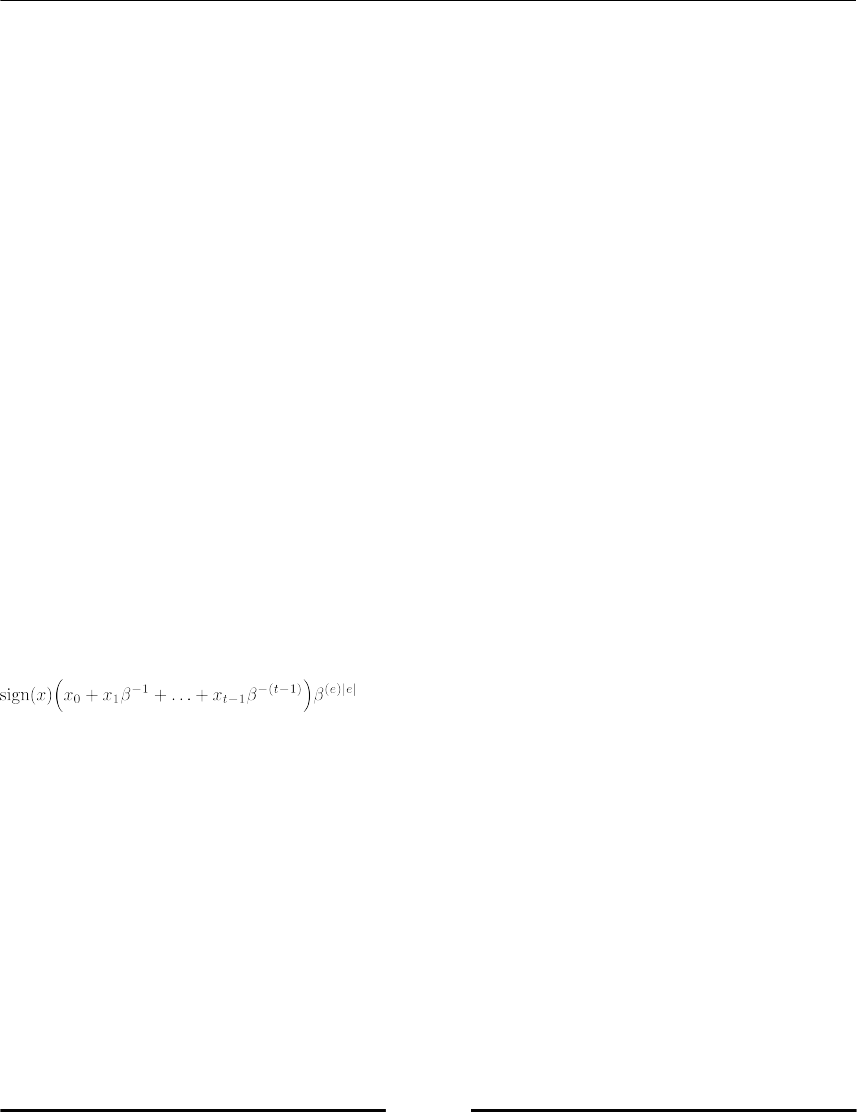
Internally, floating-point numbers are represented by four quantities: the sign, the mantissa,
the exponent sign, and the exponent:
with β ϵ ℕ and x0≠ 0, 0 ≤ xi≤ β
x0…xt-1 is called the mantissa, β the basis and e the exponent |e| ≤ U . t is called the mantissa
length. The condition x0 ≠ 0 makes the representation unique and saves, in the binary case (β
= 2), one bit.
There exist two-floating point zeros +0 and -0, both represented by the mantissa 0.
On a typical Intel processor, β = 2 . To represent a number in the float type 64 bits are
used, namely 2 bits for the signs, t = 52 bits for the mantissa and 10 bits for the exponent
|e|. The upper bound U for the exponent is consequently 210-1 = 1023.
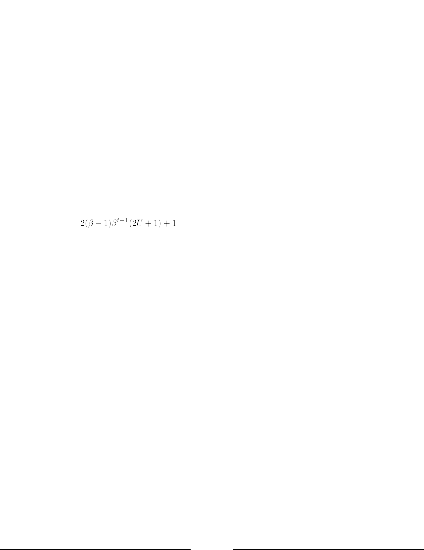
Variables and Basic Types
[ 30 ]
With this data the smallest positive representable number is
flmin = 1.0 × 2-1023≈ 10-308 and the largest is flmax = 1.111…1 × 21023≈ 10308.
Note that floating-point numbers are not equally spaced in [0, flmax]. There is in particular a
gap at zero (refer to [29]). The distance between 0 and the first positive number is 2-1023,
while the distance between the first and the second is smaller by a factor 2-52≈ 2.2 × 10⁻¹⁶. This
effect, caused by the normalization x0 ≠ 0, is visualized in Figure 2.1.
This gap is filled equidistantly with subnormal floating-point numbers to which such a
result is rounded. Subnormal floating-point numbers have the smallest possible exponent
and do not follow the convention that the leading digit x0 has to differ from zero; refer to
[13].
Infinite and not a number
There are in total floating-point numbers. Sometimes a numerical
algorithm computes floating-point numbers outside this range.
This generates number over- or underflow. In SciPy the special floating-point number inf
is assigned to overflow results:
exp(1000.) # inf
a = inf
3 - a # -inf
3 + a # inf
Working with inf may lead to mathematically undefined results. This is indicated in
Python by assigning the result another special floating-point number, nan. This stands for
not-a-number, that is, an undefined result of a mathematical operation:
a + a # inf
a - a # nan
a / a # nan
Variables and Basic Types
[ 31 ]
There are special rules for operations with nan and inf. For instance, nan compared to
anything (even to itself) always returns False:
x = nan
x < 0 # False
x > 0 # False
x == x # False
See Exercise 4 for some surprising consequences of the fact that nan is never equal to itself.
The float inf behaves much more as expected:
0 < inf # True
inf <= inf # True
inf == inf # True
-inf < inf # True
inf - inf # nan
exp(-inf) # 0
exp(1 / inf) # 1
One way to check for nan and inf is to use the isnan and isinf functions. Often, one
wants to react directly when a variable gets the value nan or inf. This can be achieved by
using the NumPy command seterr. The following command
seterr(all = 'raise')
would raise an error if a calculation were to return one of those values.
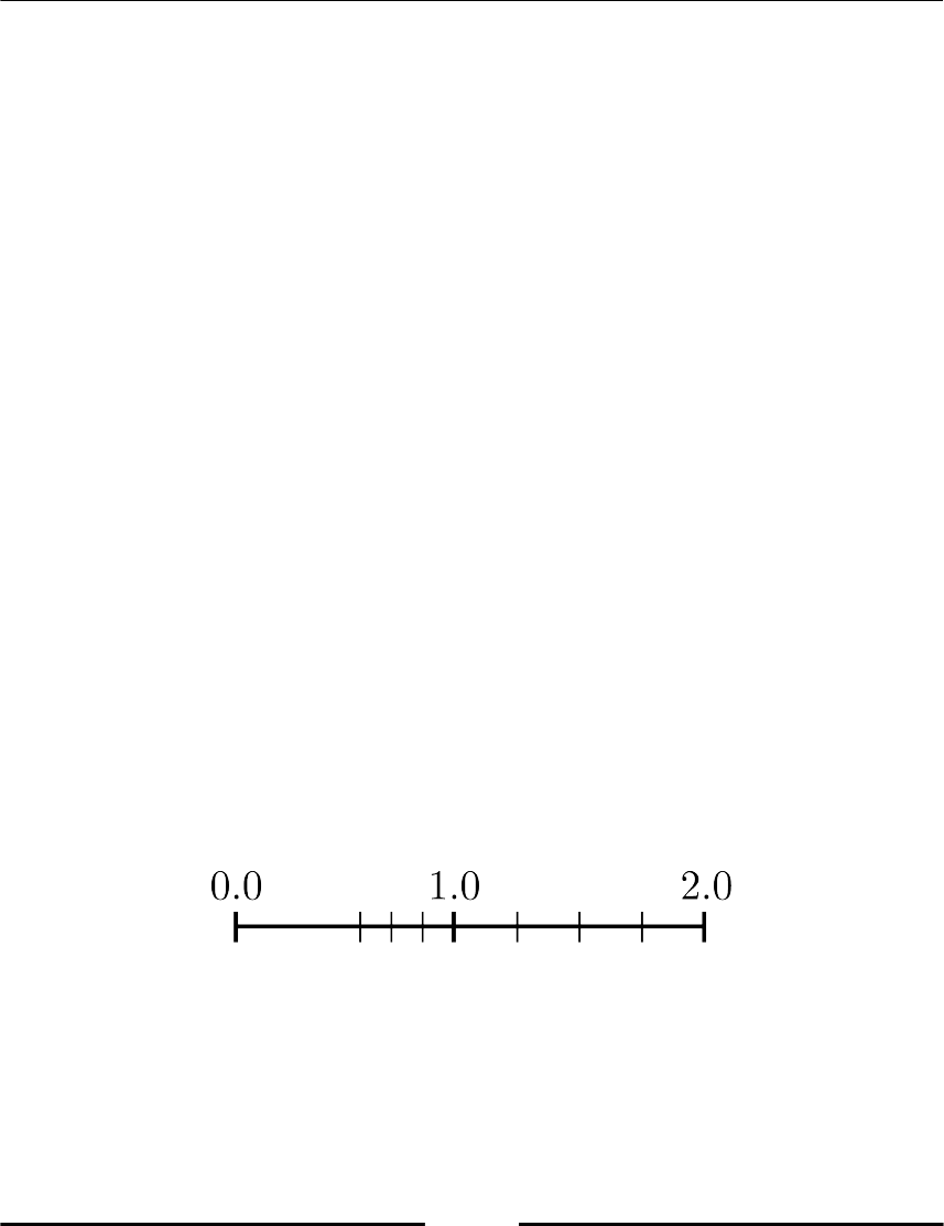
Underflow – Machine Epsilon
Underflow occurs when an operation results in a rational number that falls into the gap at
zero; refer to Figure 2.1.
Figure 2.1: The floating point gap at zero, here t = 3, U = 1
The machine epsilon or rounding unit is the largest number ε such that float(1.0 + ε) = 1.0.

Variables and Basic Types
[ 32 ]
Note that ε ≈ β1-t/2 = 1.1102 × 10⁻¹⁶ on most of today’s computers. The value that is valid on
the actual machine you are running your code on is accessible using the following
command:
import sys
sys.float_info.epsilon # 2.220446049250313e-16 (something like that)
The variable sys.float_info contains more information about the internal
representation of the float type on your machine.
The function float converts other types to a floating-point number—if possible. This
function is especially useful when converting an appropriate string to a number:
a = float('1.356')
Other float types in NumPy
NumPy also provides other float types, known from other programming languages as
double-precision and single-precision numbers, namely float64 and float32:
a = pi # returns 3.141592653589793
a1 = float64(a) # returns 3.1415926535897931
a2 = float32(a) # returns 3.1415927
a - a1 # returns 0.0
a - a2 # returns -8.7422780126189537e-08
The second last line demonstrates that a and a1 do not differ in accuracy. In the first two
lines, they only differ in the way they are displayed. The real difference in accuracy is
between a and its single-precision counterpart, a2.
The NumPy function finfo can be used to display information on these floating-point
types:
f32 = finfo(float32)
f32.precision # 6 (decimal digits)
f64 = finfo(float64)
f64.precision # 15 (decimal digits)
f = finfo(float)
f.precision # 15 (decimal digits)
f64.max # 1.7976931348623157e+308 (largest number)
f32.max # 3.4028235e+38 (largest number)
help(finfo) # Check for more options

Variables and Basic Types
[ 33 ]
Complex numbers
Complex numbers are an extension of the real numbers frequently used in many scientific
and engineering fields.
Complex Numbers in Mathematics
Complex numbers consist of two floating-point numbers, the real part a of the number and
its imaginary part b. In mathematics, a complex number is written as z=a+bi, where i defined
by i2 = -1 is the imaginary unit. The conjugate complex counterpart of z is .
If the real part a is zero, the number is called an imaginary number.
The j notation
In Python, imaginary numbers are characterized by suffixing a floating-point number with
the letter j, for example, z = 5.2j. A complex number is formed by the sum of a floating-
point number and an imaginary number, for example, z = 3.5 + 5.2j.
While in mathematics the imaginary part is expressed as a product of a real number b with
the imaginary unit i, the Python way of expressing an imaginary number is not a product: j
is just a suffix to indicate that the number is imaginary.
This is demonstrated by the following small experiment:
b = 5.2
z = bj # returns a NameError
z = b*j # returns a NameError
z = b*1j # is correct
The method conjugate returns the conjugate of z:
z = 3.2 + 5.2j
z.conjugate() # returns (3.2-5.2j)
Variables and Basic Types
[ 34 ]
Real and imaginary parts
One may access the real and imaginary parts of a complex number z using the real and
imag attributes. Those attributes are read-only:
z = 1j
z.real # 0.0
z.imag # 1.0
z.imag = 2 # AttributeError: readonly attribute
It is not possible to convert a complex number to a real number:
z = 1 + 0j
z == 1 # True
float(z) # TypeError
Interestingly, the real and imag attributes as well as the conjugate method work just as
well for complex arrays (Chapter 4, Linear Algebra – Arrays). We demonstrate this by
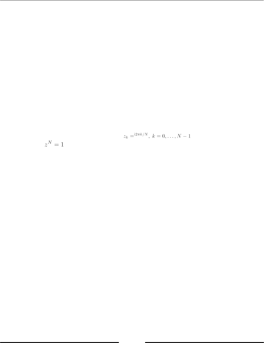
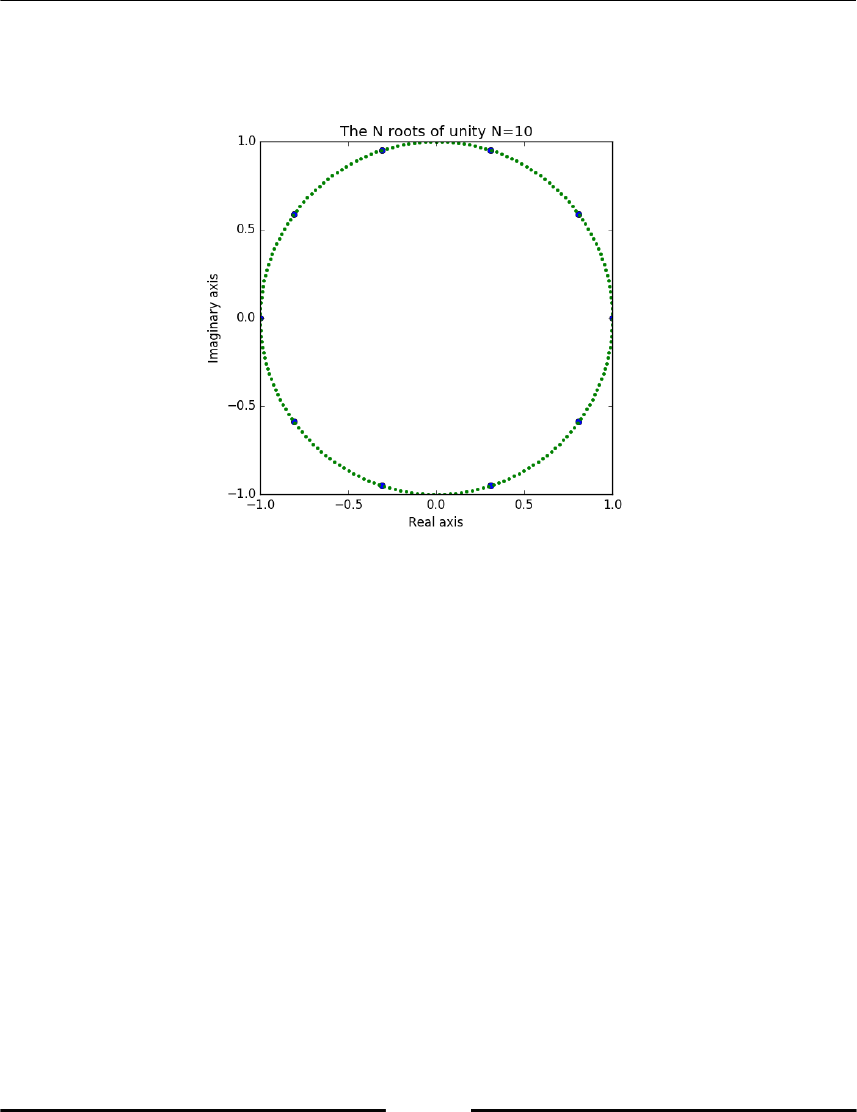
computing the Nth roots of unity which are , that is, the N solutions
of the equation :
N = 10
# the following vector contains the Nth roots of unity:
unity_roots = array([exp(1j*2*pi*k/N) for k in range(N)])
# access all the real or imaginary parts with real or imag:
axes(aspect='equal')
plot(unity_roots.real, unity_roots.imag, 'o')
allclose(unity_roots**N, 1) # True
Variables and Basic Types
[ 35 ]
The resulting figure (Figure 2.2) shows the roots of unity together with the unit circle. (For
more details on how to make plots, refer Chapter 6, Plotting.)
Figure 2.2: Roots of unity together with a unit circle
It is of course possible to mix the previous methods, as illustrated by the following
examples:
z = 3.2+5.2j
(z + z.conjugate()) / 2. # returns (3.2+0j)
((z + z.conjugate()) / 2.).real # returns 3.2
(z - z.conjugate()) / 2. # returns 5.2j
((z - z.conjugate()) / 2.).imag # returns 5.2
sqrt(z * z.conjugate()) # returns (6.1057350089894991+0j)

Variables and Basic Types
[ 36 ]
Booleans
Boolean is a datatype named after George Boole (1815-1864). A Boolean variable can take
only two values, True or False. The main use of this type is in logical expressions. Here are
some examples:
a = True
b = 30 > 45 # b gets the value False
Boolean expressions are often used in conjunction with the if statement:
if x > 0:
print("positive")
else:
print("nonpositive)
Boolean operators
Boolean operations are performed using the and, or, and not keywords in Python:
True and False # False
False or True # True
(30 > 45) or (27 < 30) # True
not True # False
not (3 > 4) # True
The operators follow some precedence rules (refer to section Executing scripts in Chapter 1,
Getting started) which would make the parentheses in the third line and in the last obsolete
(it is a good practice to use them anyway to increase the readability of your code). Note that
the and operator is implicitly chained in the following Boolean expressions:
a < b < c # same as: a < b and b < c
a == b == c # same as: a == b and b == c
Variables and Basic Types
[ 37 ]
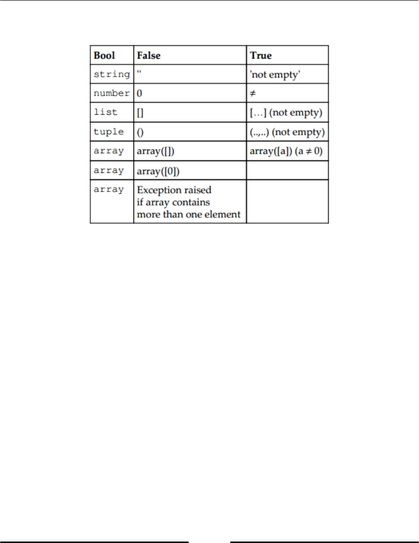
Rules of Conversion to Booleans:
Table 2.2 : Rule of conversion to Boolean
Boolean casting
Most objects Python may be converted to Booleans; this is called Boolean casting. The built-in
function bool performs that conversion. Note that most objects are cast to True, except 0,
the empty tuple, the empty list, the empty string, or the empty array. These are all cast to
False.
It is not possible to cast arrays into Booleans unless they contain no or only one element; this
is explained further in Chapter 5, Advanced Array Concepts. The previous table contains
summarized rules for Boolean casting. Some usage examples:
bool([]) # False
bool(0) # False
bool(' ') # True
bool('') # False
bool('hello') # True
bool(1.2) # True
bool(array([1])) # True
bool(array([1,2])) # Exception raised!

Variables and Basic Types
[ 38 ]
Automatic Boolean casting
Using an if statement with a non-Boolean type will cast it to a Boolean. In other words, the
following two statements are always equivalent:
if a:
...
if bool(a): # exactly the same as above
...
A typical example is testing whether a list is empty:
# L is a list
if L:
print("list not empty")
else:
print("list is empty")
An empty array, list, or tuple will return False. You can also use a variable in the if
statement, for example, an integer:
# n is an integer
if n % 2:
print("n is odd")
else:
print("n is even")
Note that we used % for the modulo operation, which returns the remainder of an integer
division. In this case, it returns 0 or 1 as the remainder after modulo 2.
In this last example, the values 0 or 1 are cast to bool. Boolean operators or,and , and not
will also implicitly convert some of their arguments to a Boolean.
Return values of and and or
Note that the operatorsand and or do not necessarily produce Boolean values. The
expression x and y is equivalent to:
def and_as_function(x,y):
if not x:
return x
else:
return y

Variables and Basic Types
[ 39 ]
And the expression x or y is equivalent to:
def or_as_function(x,y):
if x:
return x
else:
return y
Interestingly, this means that when executing the statement True or x, the variable x need
not even be defined! The same holds for False and x.
Note that, unlike their counterparts in mathematical logic, these operators are no longer
commutative in Python. Indeed, the following expressions are not equivalent:
[1] or 'a' # produces [1]
'a' or [1] # produces 'a'
Boolean and integer
In fact, Booleans and integers are the same. The only difference is in the string
representation of 0 and 1 which is in the case of Booleans False and True respectively. This
allows constructions like this (for the format method refer section on string formatting):
def print_ispositive(x):
possibilities = ['nonpositive', 'positive']
return "x is {}".format(possibilities[x>0])
We note for readers already familiar with the concept of subclasses, that the type bool is a
subclass of the type int (refer to Chapter 8, Classes). Indeed, all four inquiries
isinstance(True, bool), isinstance(False, bool), isinstance(True, int),
and isinstance(False, int) return the value True (refer to section Type Checking in
Chapter 3, Container Types).
Even rarely used statements such as True+13 are syntactically correct.
Strings
The type string is a type used for text:
name = 'Johan Carlsson'
child = "Åsa is Johan Carlsson's daughter"
book = """Aunt Julia
and the Scriptwriter"""

Variables and Basic Types
[ 40 ]
A string is enclosed either by single or double quotes. If a string contains several lines, it has
to be enclosed by three double quotes """ or three single quotes '''.
Strings can be indexed with simple indexes or slices (refer to Chapter 3, Container Types, for
a comprehensive explanation on slices):
book[-1] # returns 'r'
book[-12:] # returns 'Scriptwriter'
Strings are immutable; that is, items cannot be altered. They share this property with tuples.
The command book[1] = 'a' returns:
TypeError: 'str' object does not support item assignment
The string '\n' is used to insert a line break and 't' inserts a horizontal tabulator (TAB)
into the string to align several lines:
print('Temperature:\t20\tC\nPressure:\t5\tPa')
These strings are examples of escape sequences. Escape sequences always start with a
backslash, \ . A multi line string automatically includes escape sequences:
a="""
A multiline
example"""
a # returns '\nA multiline \nexample'
A special escape sequence is "", which represents the backslash symbol in text:
latexfontsize="\\tiny"
The same can be achieved by using a raw string instead:
latexfs=r"\tiny" # returns "\tiny"
latexfontsize == latexfs # returns True
Note that in raw strings, the backslash remains in the string and is used to escape some
special characters:
r"\"\" # returns '\\"'
r"\\" # returns '\\\\'
r"\" # returns an error
Variables and Basic Types
[ 41 ]
Operations on strings and string methods
Addition of strings means concatenation:
last_name = 'Carlsson'
first_name = 'Johanna'
full_name = first_name + ' ' + last_name
# returns 'Johanna Carlsson'
Multiplication is just repeated addition:
game = 2 * 'Yo' # returns 'YoYo'
When strings are compared, lexicographical order applies and the uppercase form precedes
the lowercase form of the same letter:
'Anna' > 'Arvi' # returns false
'ANNA' < 'anna' # returns true
'10B' < '11A' # returns true
Among the variety of string methods, we will mention here only the most important ones:
Splitting a string: This method generates a list from a string by using a single or
multiple blanks as separators. Alternatively, an argument can be given by
specifying a particular string as a separator:
text = 'quod erat demonstrandum'
text.split() # returns ['quod', 'erat', 'demonstrandum']
table = 'Johan;Carlsson;19890327'
table.split(';') # returns ['Johan','Carlsson','19890327']
king = 'CarlXVIGustaf'
king.split('XVI') # returns ['Carl','Gustaf']
Joining a list to a string: This is the reverse operation of splitting:
sep = ';'
sep.join(['Johan','Carlsson','19890327'])
# returns 'Johan;Carlsson;19890327'
Searching in a string: This method returns the first index in the string, where a
given search substring starts:
birthday = '20101210'
birthday.find('10') # returns 2
If the search string is not found, the return value of the method is -1 .

Variables and Basic Types
[ 42 ]
String formatting
String formatting is done using the format method:
course_code = "NUMA21"
print("This course's name is {}".format(course_code))
# This course's name is NUMA21
The function format is a string method; it scans the string for the occurrence of
placeholders, which are enclosed by curly brackets. These placeholders are replaced in a
way specified by the argument of the format method. How they are replaced depends on
the format specification defined in each {} pair. Format specifications are indicated by a
colon, ":", as their prefix.
The format method offers a range of possibilities to customize the formatting of objects
depending on their types. Of particular use in scientific computing are the formatting
specifiers for the float type. One may choose either the standard with {:f} or the
exponential notation with {:e}:
quantity = 33.45
print("{:f}".format(quantity)) # 33.450000
print("{:1.1f}".format(quantity)) # 33.5
print("{:.2e}".format(quantity)) # 3.35e+01
The format specifiers allow to specify the rounding precision (digits following the decimal
point in the representation). Also the total number of symbols including leading blanks to
represent the number can be set.
In this example, the name of the object that gets its value inserted is given as an argument to
the format method. The first {} pair is replaced by the first argument and the following
pairs by the subsequent arguments. Alternatively, it may also be convenient to use the key-
value syntax:
print("{name} {value:.1f}".format(name="quantity",value=quantity))
# prints "quantity 33.5"
Here, two values are processed, a string name without a format specifier and a float
value that is printed in fixed point notation with one digit after the decimal point. (We
refer to the complete reference documentation for more details on string formatting, [34]).
Variables and Basic Types
[ 43 ]
Braces in the string
Sometimes, a string might contain a pair of curly braces, which should not
be considered as placeholders for a format method. In that case, double
braces are used:
r"we {} in LaTeX \begin{{equation}}".format('like')
This returns the following string: 'we like in LaTeX
\\begin{equation}'.
Summary
In this chapter, you met the basic data types in Python and saw the corresponding syntax
elements. We will work mostly with numeric types such as integers, floats and complex.
Booleans are needed for setting conditions, and by using strings, we often communicate
results and messages.
Exercises
Ex. 1 → Check whether x = 2.3 is a zero of the function:
Ex. 2 → According to de Moivre's formula, the following holds:
Choose numbers n and x and verify that formula in Python.
Ex. 3 → Complex numbers. Verify Euler's formula in the same way:

Variables and Basic Types
[ 44 ]
Ex. 4 → Suppose we are trying to check the convergence of a diverging sequence (here the
sequence is defined by the recursive relation un+1 = 2un and u0 = 1.0):
u = 1.0 # you have to use a float here!
uold = 10.
for iteration in range(2000):
if not abs(u-uold) > 1.e-8:
print('Convergence')
break # sequence has converged
uold = u
u = 2*u
else:
print('No convergence')
Since the sequence does not converge, the code should print the No1.
convergence message. Execute it to see what happens.
What happens if you replace the line:2.
if not abs(u-uold) > 1.e-8
with:
if abs(u-uold) < 1.e-8
It should give exactly the same result, shouldn't it? Run the code again to see
what happens.
What happens if you replace u=1.0 by u=1 (without decimal point). Run the code3.
to check your predictions.
Explain the unexpected behavior of this code. The key to understand what4.
happens is that inf evaluates to nan, and the comparison of nan with anything
else is returns always the value False .
Ex. 5 → An implication C = (A ⇒ B) is a Boolean expression that is defined as
C is True if A is False or A and B are both True
C is False otherwise
Write a Python function implication(A, B).
Variables and Basic Types
[ 45 ]
Ex. 6 → This exercise is to train Boolean operations. Two binary digits (bits) are added by
using a logical device called a half adder. It produces a carry bit (the digit of the next higher
value) and the sum as defined by the following table, and half adder circuit.
p q sum carry
1101
1010
01 1 0
0 0 0 0
Definition of the half adder operation
Figure 2.3: A half adder circuit
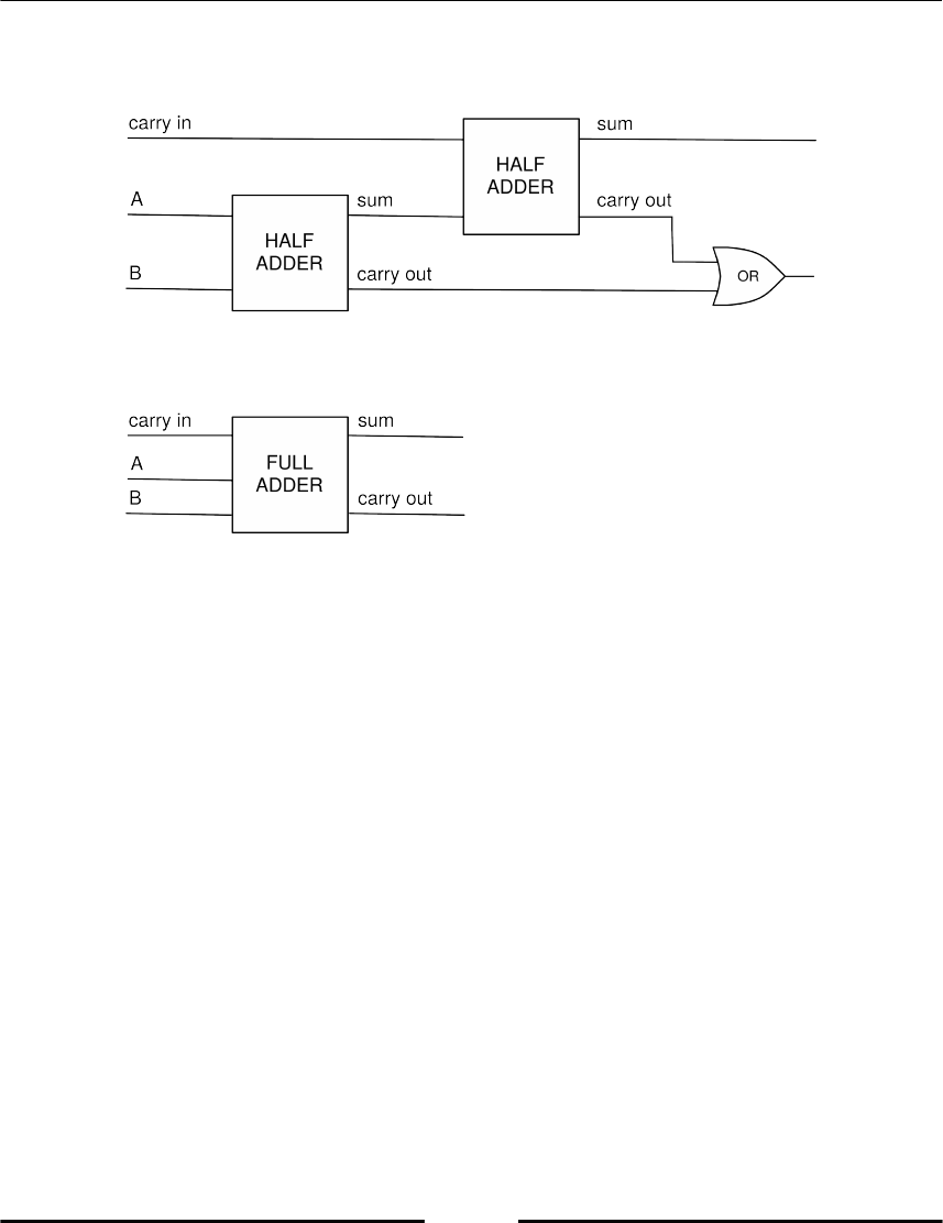
Variables and Basic Types
[ 46 ]
A full adder consists of two half adders and sums up two bits and an additional carry bit on
the input (refer to the following figure):
Figure 2.4: A full adder circuit
Write a function that implements a half adder and another that implements a full adder.
Test these functions.
3
Container Types
Container types are used to group objects together. The main difference between the
different container types is the way individual elements are accessed and how operations
are defined.
Lists
A list is, as the name hints, a list of objects of any kind:
L = ['a' 20.0, 5]
M = [3,['a', -3.0, 5]]
The individual objects are enumerated by assigning each element an index. The first
element in the list gets index 0. This zero-based indexing is frequently used in mathematical
notation. Consider the usual indexing of coefficients of a polynomial.
The index allows us to access the following objects:
L[1] # returns 20.0
L[0] # returns 'a'
M[1] # returns ['a',-3.0,5]
M[1][2] # returns 5
The bracket notation here corresponds to the use of subscripts in mathematical formulas. L
is a simple list, while M itself contains a list so that one needs two indexes to access an
element of the inner list.
A list containing subsequent integers can easily be generated by the command range:
L=list(range(4)) # generates a list with four elements: [0, 1, 2 ,3]
Container Types
[ 48 ]
A more general use is to provide this command with start, stop, and step parameters:
L=list(range(17,29,4)) # generates [17, 21, 25]
The command len returns the length of the list:
len(L) # returns 3
Slicing
Slicing a list between i and j creates a new list containing the elements starting at index
i and ending just before j.
For slicing, a range of indexes has to be given. L[i:j] means create a list by taking all
elements from L starting at L[i] until L[j-1]. In other words, the new list is obtained by
removing the first i elements from L and taking the next j-i elements (for j > i ≥ 0). See
the following figure (Figure 3.1) for more examples:
Figure 3.1: Some typical slicing situations
Container Types
[ 49 ]
Here, L[i:] means remove the i first elements, L[:i] means take only the first i elements,
and similarly, L[:-i] means remove the last i elements, and L[-i:] means take only the
last i elements. This may be combined in L[i:-j] to remove the first i and the last j
elements:
L = ['C', 'l', 'o', 'u', 'd', 's']
L[1:5] # remove one element and take four from there:
# returns ['l', 'o', 'u', 'd']
One may omit the first or last bound of the slicing:
L = ['C', 'l', 'o', 'u','d', 's']
L[1:] # ['l', 'o', 'u', 'd','s']
L[:5] # ['C', 'l', 'o','u','d']
L[:] # the entire list
Python allows the use of negative indexes for counting from the right. In particular, the
element L[-1] is the last element in the list L.
Some list indexing descriptions:
L[i:] amounts to taking all elements except the i first ones
L[:i] amounts to taking the first i elements
L[-i:] amounts to taking the last i elements
L[:-i] amounts to taking all elements except the i last ones
Here is an example:
L = ['C', 'l', 'o', 'u', 'd', 's']
L[-2:] # ['d', 's']
L[:-2] # ['C', 'l', 'o','u']
Omitting one index in the range corresponds to half-open intervals in ℝ. The half-open
interval (∞, a) means, take all numbers strictly lower than a; this is similar to the syntax
L[:j].
Out of-bound slices
Notice that you never get index errors with out-of-bound slices. Possibly,
you may obtain empty lists.

Container Types
[ 50 ]
Here is an example:
L = list(range(4)) # [0, 1, 2, 3]
L[4] # IndexError: list index out of range
L[1:100] # same as L[1:]
L[-100:-1] # same as L[:-1]
L[-100:100] # same as L[:]
L[5:0] # empty list []
L[-2:2] # empty list []
Be careful when using variables in indexing that may become negative, since it changes the
slice completely. This might lead to unexpected results:
a = [1,2,3]
for iteration in range(4):
print(sum(a[0:iteration-1]))
The result is 3, 0, 1, 3 while one expects 0, 0, 1, 3.
Strides
When computing slices, one may also specify a stride, which is the length of the step from
one index to the other. The default stride is one. Here is an example:
L = list(range(100))
L[:10:2] # [0, 2, 4, 6, 8]
L[::20] # [0, 20, 40, 60, 80]
L[10:20:3] # [10, 13, 16, 19]
Note that the stride may also be negative:
L[20:10:-3] # [20, 17, 14, 11]
It is also possible to create a new list that is reversed, using a negative stride (find about
reverse method in section In-place operations):
L = [1, 2, 3]
R = L[::-1] # L is not modified
R # [3, 2, 1]

Container Types
[ 51 ]
Altering lists
Typical operations on lists are insertion and deletion of elements and list concatenation.
With the slicing notation, list insertion and deletion become obvious; deletion is just
replacing a part of a list by an empty list []:
L = ['a', 1, 2, 3, 4]
L[2:3] = [] # ['a', 1, 3, 4]
L[3:] = [] # ['a', 1, 3]
Insertion means replacing an empty slice with the list to be inserted:
L[1:1] = [1000, 2000] # ['a', 1000, 2000, 1, 3]
Two lists are concatenated by the plus operator + :
L = [1, -17]
M = [-23.5, 18.3, 5.0]
L + M # gives [1, -17, 23.5, 18.3, 5.0]
Concatenating a list n times with itself motivates the use of the multiplication operator *:
n = 3
n * [1.,17,3] # gives [1., 17, 3, 1., 17, 3, 1., 17, 3]
[0] * 5 # gives [0,0,0,0,0]
There is no arithmetic operations on list, such as elementwise summation or division. For
such operations we use arrays (refer to section Array).
Belonging to a list
One may use the keywords in and not in to determine whether an element belongs to a
list or not which is similar to and in mathematics:
L = ['a', 1, 'b', 2]
'a' in L # True
3 in L # False
4 not in L # True
Container Types
[ 52 ]
List methods
Some useful methods of the list type are collected in the following Table 3.1:
Command Action
list.append(x) Add x to the end of the list.
list.expand(L) Expand the list by the elements of the list L.
list.insert(i,x) Insert x at positioni.
list.remove(x) Remove the first item from the list whose value is x.
list.count(x) The number of times x appears in the list.
list.sort() Sort the items of the list, in place.
list.reverse() Reverse the elements of the list, in place.
list.pop() Remove the last element of the list, in place.
Table 3.1: Methods of the datatype list
There are two ways list methods can act:
They can directly alter the list, that is, in-place operations.
They produce a new object.
In–place operations
All methods that result in a list are in-place operating methods, for example, reverse:
L = [1, 2, 3]
L.reverse() # the list
L is now reversed
L # [3, 2, 1]
Be aware of in-place operations. One might be tempted to write:
L=[3, 4, 4, 5]
newL = L.sort()
This is correct Python. But it results in a possibly unintended alternation of L in a variable
newL having the value None. The reason is that sort operates in-place.

Container Types
[ 53 ]
Here we demonstrate in-place operating methods:
L = [0, 1, 2, 3, 4]
L.append(5) # [0, 1, 2, 3, 4, 5]
L.reverse() # [5, 4, 3, 2, 1, 0]
L.sort() # [0, 1, 2, 3, 4, 5]
L.remove(0) # [1, 2, 3, 4, 5]
L.pop() # [1, 2, 3, 4]
L.pop() # [1, 2, 3]
L.extend(['a','b','c']) # [1, 2, 3, 'a', 'b', 'c']
L is altered. The count method is an example of a method that generates a new object:
L.count(2) # returns 1
Merging lists – zip
A particularly useful function for lists is zip. It can be used to merge two given lists into a
new list by pairing the elements of the original lists. The result is a list of tuples (refer
section Tuples for more information):
ind = [0,1,2,3,4]
color = ["red", "green", "blue", "alpha"]
list(zip(color,ind)) # gives [('red', 0), ('green', 1),
('blue', 2), ('alpha', 3)]
This example also demonstrates what happens if the lists have different lengths. The length
of the zipped list is the shorter of the two input lists.
zip creates a special iterable object that can be turned into a list by applying the list
function, as in the preceding example. Refer to section Iterators in Chapter 9, Iterating, for
more details on iterable objects.
List comprehension
A convenient way to build up lists is by using the list comprehension construct, possibly
with a condition inside. The syntax of a list comprehension is:
[<expr> for <variable> in <list>]

Container Types
[ 54 ]
or more generally:
[<expr> for <variable> in <list> if <condition>]
Here is an example:
L = [2, 3, 10, 1, 5]
L2 = [x*2 for x in L] # [4, 6, 20, 2, 10]
L3 = [x*2 for x in L if 4 < x <= 10] # [20, 10]
It is possible to have several for loops inside a list comprehension:
M = [[1,2,3],[4,5,6]]
flat = [M[i][j] for i in range(2) for j in range(3)]
# returns [1, 2, 3, 4, 5, 6]
This is of particular interest when dealing with arrays.
Set notation
List comprehension is closely related to the mathematical notation for sets.
Compare: and L2 = [2*x for x in L].
One big difference though, is that lists are ordered while sets aren't (Refer,
section Sets for more information).
Arrays
The NumPy package offers arrays, which are container structures for manipulating vectors,
matrices, or even higher order tensors in mathematics. In this section, we point out the
similarities between arrays and lists. But arrays deserve a broader presentation, which will
be given in Chapter 4, Linear Algebra – Arrays, and Chapter 5, Advanced Array Concepts.
Arrays are constructed from lists by the function array :
v = array([1.,2.,3.])
A = array([[1.,2.,3.],[4.,5.,6.]])
To access an element of a vector, we need one index, while an element of a matrix is
addressed by two indexes:
v[2] # returns 3.0
A[1,2] # returns 6.0
Container Types
[ 55 ]
At first glance, arrays are similar to lists, but be aware that they are different in a
fundamental way, which can be explained by the following points:
Access to array data corresponds to that of lists, using square brackets and slices.
They may also be used to alter the array:
M = array([[1.,2.],[3.,4.]])
v = array([1., 2., 3.])
v[0] # 1
v[:2] # array([1.,2.])
M[0,1] # 2
v[:2] = [10, 20] # v is now array([10., 20., 3.])
The number of elements in a vector, or the number of rows of a matrix, is
obtained by the function len :
len(v) # 3
Arrays store only elements of the same numeric type (usually float or complex
but also int). Refer to section Array properties in Chapter 4, Liner Algebra –
Arrays, for more information.
The operations +, *, /, and - are all elementwise. The dot function and, in
Python versions ≥ 3.5, the infix operator @ are used for the scalar product and the
corresponding matrix operations.
Unlike lists, there is no append method for arrays. Nevertheless, there are special
methods to construct arrays by stacking smaller size arrays (Refer to section
Stacking in Chapter 4, Linear Algebra – Arrays, for more information.). A related
point is that arrays are not elastic as lists; one cannot use slices to change their
length.
Vector slices are views; that is, they may be used to modify the original array.
Refer to section Array views and copies in Chapter 5, Advanced Array Concepts, for
more information.

Container Types
[ 56 ]
Tuples
A tuple is an immutable list. Immutable means that it cannot be modified. A tuple is just a
comma-separated sequence of objects (a list without brackets). To increase readability, one
often encloses a tuple in a pair of parentheses:
my_tuple = 1, 2, 3 # our first tuple
my_tuple = (1, 2, 3) # the same
my_tuple = 1, 2, 3, # again the same
len(my_tuple) # 3, same as for lists
my_tuple[0] = 'a' # error! tuples are immutable
The comma indicates that the object is a tuple:
singleton = 1, # note the comma
len(singleton) # 1
Tuples are useful when a group of values goes together; for example, they are used to
return multiple values from functions (refer to section Returns Values in Chapter 7,
Functions. One may assign several variables at once by unpacking a list or tuple:
a, b = 0, 1 # a gets 0 and b gets 1
a, b = [0, 1] # exactly the same effect
(a, b) = 0, 1 # same
[a,b] = [0,1] # same thing
The swapping trick
Use packing and unpacking to swap the contents of two variables:
a, b = b, a
To summarize:
Tuples are nothing other than immutable lists with a notation without brackets.
In most cases, lists may be used instead of tuples.
The notation without parentheses is convenient but dangerous. You should use
parentheses when you are not sure:
a, b = b, a # the swap trick; equivalent to:
(a, b) = (b, a)
# but
1, 2 == 3, 4 # returns (1, False, 4)
(1, 2) == (3, 4) # returns False

Container Types
[ 57 ]
Dictionaries
Lists, tuples, and arrays are ordered sets of objects. The individual objects are inserted,
accessed, and processed according to their place in the list. On the other hand, dictionaries
are unordered sets of pairs. One accesses dictionary data by keys.
Creating and altering dictionaries
For example, we may create a dictionary containing the data of a rigid body in mechanics,
as follows:
truck_wheel = {'name':'wheel','mass':5.7,
'Ix':20.0,'Iy':1.,'Iz':17.,
'center of mass':[0.,0.,0.]}
A key/data pair is indicated by a colon, :. These pairs are comma separated and listed
inside a pair of curly brackets, {}.
Individual elements are accessed by their keys:
truck_wheel['name'] # returns 'wheel'
truck_wheel['mass'] # returns 5.7
New objects are added to the dictionary by creating a new key:
truck_wheel['Ixy'] = 0.0
Dictionaries are also used to provide parameters to a function (refer to section Parameters
and arguments in Chapter 7, Functions, for further information). Keys in a dictionary can be,
among others, strings, functions, tuples with immutable elements, and classes. Keys cannot
be lists or arrays. The command dict generates a dictionary from a list with key/value
pairs:
truck_wheel = dict([('name','wheel'),('mass',5.7),('Ix',20.0),
('Iy',1.), ('Iz',17.),
('center of mass',[0.,0.,0.])])
The zip function may come in handy in this context (refer to section Merging List).
Container Types
[ 58 ]
Looping over dictionaries
There are mainly three ways to loop over dictionaries:
By keys:
for key in truck_wheel.keys():
print(key) # prints (in any order) 'Ix', 'Iy', 'name',...
or equivalently:
for key in truck_wheel:
print(key) # prints (in any order) 'Ix', 'Iy', 'name',...
By value:
for value in truck_wheel.value():
print(value)
# prints (in any order) 1.0, 20.0, 17.0, 'wheel', ...
By item, that is, key/value pairs:
for item in truck_wheel.items():
print(item)
# prints (in any order) ('Iy', 1.0), ('Ix, 20.0),...
Please, refer to section Shelves in Chapter 12, Input and Output, for a special dictionary
object for file access.
Sets
Sets are containers that share properties and operations with sets in mathematics. A
mathematical set is a collection of distinct objects. Here are some mathematical set
expressions:

Container Types
[ 59 ]
And their Python counterparts:
A = {1,2,3,4}
B = {5}
C = A.union(B) # returns set([1,2,3,4,5])
D = A.intersection(C) # returns set([1,2,3,4])
E = C.difference(A) # returns set([5])
5 in C # returns True
Sets contain an element only once, corresponding to the aforementioned definition:
A = {1,2,3,3,3}
B = {1,2,3}
A == B # returns True
And a set is unordered; that is, the order of the elements in the set is not defined:
A = {1,2,3}
B = {1,3,2}
A == B # returns True
Sets in Python can contain all kinds of hashable objects, that is, numeric objects, strings, and
Booleans.
There are union and intersection methods:
A={1,2,3,4}
A.union({5})
A.intersection({2,4,6}) # returns set([2, 4])
Also, sets can be compared using the methods issubset and issuperset :
{2,4}.issubset({1,2,3,4,5}) # returns True
{1,2,3,4,5}.issuperset({2,4}) # returns True
Empty set
An empty set is defined in Python by empty_set=set([]) and not by {},
which would define an empty dictionary!

Container Types
[ 60 ]
Container conversions
We summarize in the following Table 3.2 the most important properties of the container
types presented so far. Arrays will be treated in Chapter 4, Linear Algebra – Arrays.
Table 3.2 : Container Types
As you can see in the previous table, there is a difference in accessing container elements,
and sets and dictionaries are not ordered.
Due to the different properties of the various container types, we frequently convert one
type to another:

Container Types
[ 61 ]
Type checking
The direct way to see the type of a variable is to use the type command:
label = 'local error'
type(label) # returns str
x = [1, 2] # list
type(x) # returns list
However, if you want to test for a variable to be of a certain type, you should use
isinstance (instead of comparing the types with type):
isinstance(x, list) # True
The reason for using isinstance becomes apparent after having read Chapter 8,
Classes, and in particular the concept of subclassing and inheritance in section Subclassing
and Inheritance in Chapter 8, Classes. In short, often different types share some common
properties with some basic type. The classical example is the type bool, which is derived by
subclassing from the more general type int. In this situation, we see how the command
isinstance can be used in a more general way:
test = True
isinstance(test, bool) # True
isinstance(test, int) # True
type(test) == int # False
type(test) == bool # True
So, in order to make sure that the variable test is as good as an integer (the particular type
may be irrelevant), you should check that it is an instance of integer:
if isinstance(test, int):
print("The variable is an integer")
Type checking
Python is not a typed language. What that means is that objects are
identified by what they can do rather than what they are. For instance, if
you have a string manipulating function that acts on an object by using
the len method, then your function will probably be useful for any objects
implementing that method.
So far, we have come across different types: float, int, bool, complex, list, tuple,
module, function, str, dict, and array.

Container Types
[ 62 ]
Summary
In this chapter, you learned to work with container types, mainly lists. It is important to
know how to fill these containers and how to access their content. We saw that there is
access by position or by keyword.
We will meet the important concept of slicing again in the next chapter on arrays. These are
containers specially designed for mathematical operations.
Exercises
Ex. 1 → Execute the following statements:
L = [1, 2]
L3 = 3*L
What is the content of L3?1.
Try to predict the outcome of the following commands:2.
L3[0]
L3[-1]
L3[10]
What does the following command do?3.
L4 = [k**2 for k in L3]
Concatenate L3 and L4 to a new list L5.4.
Ex. 2 → Use the range command and a list comprehension to generate a list with 100
equidistantly spaced values between 0 and 1.
Ex. 3 → Assume that the following signal is stored in a list:
L = [0,1,2,1,0,-1,-2,-1,0]

Container Types
[ 63 ]
What is the outcome of:
L[0]
L[-1]
L[:-1]
L + L[1:-1] + L
L[2:2] = [-3]
L[3:4] = []
L[2:5] = [-5]
Do this exercise by inspection only, that is, without using your Python Shell.
Ex. 4 → Consider the Python statements:
L = [n-m/2 for n in range(m)]
ans = 1 + L[0] + L[-1]
and assume that the variable m has been previously assigned an integer value. What is the
value of ans? Answer this question without executing the statements in Python.
Ex. 5 → Consider the recursion formula:
with n = 0,…, 1000, h= 1/1000, and a = -0.5.
Create a list u. Store in its first three elements e0, eha, and e2ha. These represent the1.
starting values u0, u1, and u2 in the given formula. Build up the complete list from
the recursion formula.
Construct a second list, td, in which you store the values nh, with n = 0, …, 1000.2.
Plot td versus u (refer section Basic plotting in Chapter 6, Plotting, for more
information). Make a second plot in which you plot the difference, that is, |eatn–
un|, where tn represents the values inside the vector td . Set axis labels and a title.
The recursion is a multistep formula to solve the differential equation u' = au with the initial
value u(0) = u0 = 1. un approximates u(nh) = eanhu0.

Container Types
[ 64 ]
Ex. 6 → Let A and B be sets. The set (A \ B) ∪ (B \ A) is called the symmetric difference of
the two sets. Write a function that performs this operation. Compare your results to the
result of the command:
A.symmetric_difference(B).
Ex. 7 → Verify in Python the statement that the empty set is a subset of any set.
Ex. 8 → Study other operations on sets. You find a complete list of those by using the
command completion feature of IPython. In particular, study the update and
intersection_update methods. What is the difference between intersection and
intersection_update?
4
Linear Algebra – Arrays
Linear algebra is one of the essential building blocks of computational mathematics. The
objects of linear algebra are vectors and matrices. The package NumPy includes all the
necessary tools to manipulate those objects.
The first task is to build matrices and vectors, or to alter existing ones by slicing. The other
main task is the dot operation, which embodies most of the linear algebra operations (scalar
product, matrix-vector product, and matrix-matrix product). Finally, various methods are
available to solve linear problems.
Overview of the array type
For the impatient, here is how to use arrays in a nutshell. Be aware though that the behavior
of arrays may be surprising at first, so we encourage you to read on after this introductory
section.
Vectors and matrices
Creating vectors is as simple as using the function array to convert a list to an array:
v = array([1.,2.,3.])
The object v is now a vector that behaves much like a vector in linear algebra. We have
already emphasized the differences with the list object in Python (refer to section Arrays in
Chapter 3, Containers Type). Here are some illustrations of the basic linear algebra
operations on vectors:
# two vectors with three components
v1 = array([1., 2., 3.])

Linear Algebra – Arrays
[ 66 ]
v2 = array([2, 0, 1.])
# scalar multiplications/divisions
2*v1 # array([2., 4., 6.])
v1/2 # array([0.5, 1., 1.5])
# linear combinations
3*v1 # array([ 3., 6., 9.])
3*v1 + 2*v2 # array([ 7., 6., 11.])
# norm
from scipy.linalg import norm
norm(v1) # 3.7416573867739413
# scalar product
dot(v1, v2) # 5.
v1 @ v2 # 5 ; alternative formulation
Note that all basic arithmetic operations are performed elementwise:
# elementwise operations:
v1 * v2 # array([2., 0., 3.])
v2 / v1 # array([2.,0.,.333333])
v1 - v2 # array([-1., 2., 2.])
v1 + v2 # array([ 3., 2., 4.])
Some functions act elementwise on arrays as well:
cos(v1) # cosine, elementwise: array([ 0.5403,
-0.4161, -0.9899])
This subject will be covered in the section Functions Acting on Arrays.
A matrix is created in a similar way to a vector, but from a list of lists instead:
M = array([[1.,2],[0.,1]])
Vectors are no column – and no row matrices
The n vector, an n × 1, and a 1 × n matrix are three different objects even if
they contain the same data.
To create a row matrix containing the same data as the vector v = array([1., 2., 1.]),
we do this:
R = array([[1.,2.,1.]]) # notice the double brackets:
# this is a matrix
shape(R) # (1,3): this is a row matrix

Linear Algebra – Arrays
[ 67 ]
The corresponding column matrix is obtained by the method reshape:
C = array([1., 2., 1.]).reshape(3, 1)
shape(C) # (3,1): this is a column matrix
Indexing and slices
Indexing and slicing are similar to that of a list. The main difference is that there may be
several indexes or slices when the array is a matrix. The subject will be covered in depth in
section Array indexing; here, we just give some illustrating examples of indexing and slicing:
v = array([1., 2., 3])
M = array([[1., 2],[3., 4]])
v[0] # works as for lists
v[1:] # array([2., 3.])
M[0, 0] # 1.
M[1:] # returns the matrix array([[3., 4]])
M[1] # returns the vector array([3., 4.])
# access
v[0] # 1.
v[0] = 10
# slices
v[:2] # array([10., 2.])
v[:2] = [0, 1] # now v == array([0., 1., 3.])
v[:2] = [1, 2, 3] # error!
Linear algebra operations
The essential operator that performs most of the usual operations of linear algebra is the
Python function dot. It is used for matrix-vector multiplications:
dot(M, v) # matrix vector multiplication; returns a vector
M @ v # alternative formulation
It may be used to compute a scalar product between two vectors:
dot(v, w) # scalar product; the result is a scalar
v @ w # alternative formulation
Linear Algebra – Arrays
[ 68 ]
Lastly, it is used to compute matrix-matrix products:
dot(M, N) # results in a matrix
M @ N # alternative formulation
Solving a linear system
If A is a matrix and b is a vector, you can solve the linear equation:
Using the solve method, which has this syntax:
from scipy.linalg import solve
x = solve(A, b)
For example, we want to solve:
Here is the solution for the preceding equation:
from scipy.linalg import solve
A = array([[1., 2.], [3., 4.]])
b = array([1., 4.])
x = solve(A, b)
allclose(dot(A, x), b) # True
allclose(A @ x, b) # alternative formulation
The command allclose is used here to compare two vectors. If they are close enough to
each other, this command returns True. Optionally a tolerance value can be set. For more
methods related to linear equations systems, refer to section Linear algebra methods in SciPy.
Linear Algebra – Arrays
[ 69 ]
Mathematical preliminaries
In order to understand how arrays work in NumPy, it is useful to understand the
mathematical parallel between accessing tensor (matrix and vector) elements by indexes
and evaluating mathematical functions by providing arguments. We also cover in this
section the generalization of the dot product as a reduction operator.
Arrays as functions
Arrays may be considered from several different points of view. We believe that the most
fruitful one in order to understand arrays is that of functions of several variables.
For instance, selecting a component of a given vector in ℝn may just be considered a
function from the set of ℕn to ℝ, where we define the set:
Here the set ℕn has n elements. The Python function range generates ℕn.
Selecting an element of a given matrix, on the other hand, is a function of two parameters,
taking its value in ℝ. Picking a particular element of an m × n matrix may thus be
considered a function from ℕm × ℕn to ℝ.
Operations are elementwise
NumPy arrays are essentially treated as mathematical functions. This is in particular true
for operations. Consider two functions, f and g, defined on the same domain and taking real
values. The product f g of those two functions is defined as the pointwise product, that is:
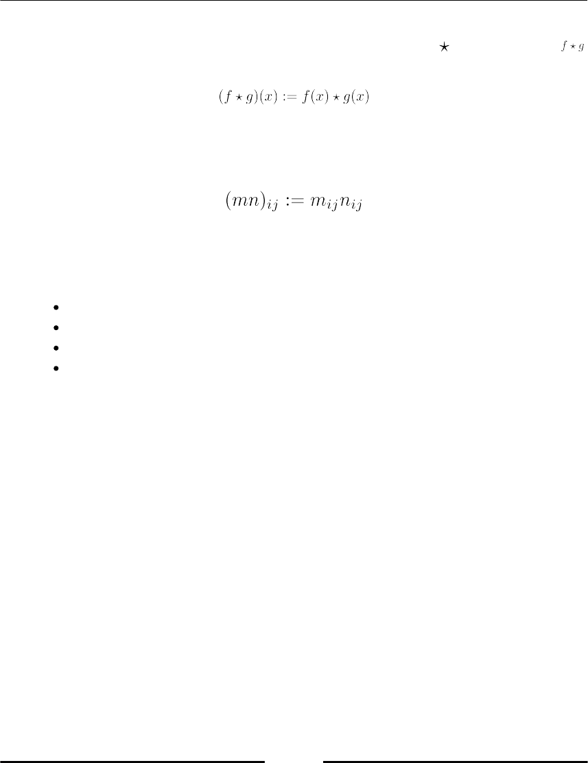
Linear Algebra – Arrays
[ 70 ]
Note that this construction is possible for any operation between two functions. For an
arbitrary operation defined on two scalars, which we denote here by , we could define
as follows:
This innocuous remark allows us to understand NumPy's stance on operations; all
operations are elementwise in arrays. For instance, the product between two matrices m and
n is defined, as with functions, as follows:
Shape and number of dimensions
There is a clear distinction between a:
Scalar: Function with no arguments
Vector: Function with one argument
Matrix: Function with two arguments
Higher order tensor: Function with more than two arguments
In what follows, the number of dimensions is the number of arguments of a function. The
shape corresponds essentially to the domain of definition of a function.
For instance, a vector of size n is a function from the set ℕn to ℝ. As a result, its domain of
definition is ℕn. Its shape is defined as the singleton (n,). Similarly, a matrix of size m × n is a
function defined on ℕm × ℕm. The corresponding shape is simply the pair (m, n). The shape of
an array is obtained by the numpy.shape function, and the number of dimensions by the
numpy.ndim function.
Linear Algebra – Arrays
[ 71 ]
The dot operations
Treating arrays as functions, although very powerful, completely neglects the linear algebra
structures we are familiar with, that is, matrix-vector and matrix-matrix
operations. Fortunately, these linear algebra operations may all be written in a similar
unified form:
The vector-vector operation:
The matrix-vector operation:
The matrix-matrix operation:
The vector-matrix operation:
The essential mathematical concept is that of reduction. For a matrix-vector operation, the
reduction is given by:
In general, a reduction operation defined between two tensors T and U of respective
number of dimensions m and n may be defined as:
Linear Algebra – Arrays
[ 72 ]
Clearly, the shapes of the tensors must be compatible for that operation to make any sense.
This requirement is familiar for matrix-matrix multiplication. The multiplication M N of
matrices M and N only makes sense if the number of columns of M equals the number of
rows of N.
Another consequence of the reduction operation is that it produces a new tensor with m + n
– 2 dimensions. In the following table, we gather the output of the reduction operation for
the familiar cases involving matrices and vectors:
Table 4.1: Output of the reduction operation for the familiar cases involving matrices and
vectors
In Python, all reduction operations are performed using the dot function:
angle = pi/3
M = array([[cos(angle), -sin(angle)],
[sin(angle), cos(angle)]])
v = array([1., 0.])
y = dot(M, v)
As in mathematical textbooks, also in modern Python (Version 3.5 and higher), the dot
product is sometimes preferred to be written in its operator form, dot(M, v), or by using
the more handy infix notation, M @ v. From now on we stick to the operator form; you can
modify the examples if the other form is preferred.
Elementwise versus matrix multiplication
The multiplication operator * is always elementwise. It has nothing to do
with the dot operation. Even if A is a matrix and v is a vector, A*v is still a
legal operation.
The matrix-vector multiplication is performed using the dot function.
Refer to section Broadcasting of Chapter 5, Advanced Array Concepts, for
more information.

Linear Algebra – Arrays
[ 73 ]
The array type
The objects used to manipulate vectors, matrices, and more general tensors in NumPy are
called arrays. In this section, we examine their essential properties, how to create them, and
how to access their information.
Array properties
Arrays are essentially characterized by three properties, which is given in the following
table (Table 4.2):
Name Description
shape It describes how the data should be interpreted, as a vector, a matrix or as a higher
order tensor, and it gives the corresponding dimension. It is accessed with the
shape attribute.
dtype It gives the type of the underlying data (float, complex, integer, and so on).
strides This attribute specifies in which order the data should be read. For instance, a
matrix could be stored in memory contiguously column by column (the FORTRAN
convention), or row by row (the C convention). The attribute is a tuple with the
numbers of bytes that have to be skipped in memory to reach the next row and the
number of bytes to be skipped to reach the next column. The strides attribute
even allows for a more flexible interpretation of the data in memory, which is what
makes array views possible.
Table 4.2 : Properties of Arrays
Consider the following array:
A = array([[1, 2, 3], [3, 4, 6]])
A.shape # (2, 3)
A.dtype # dtype('int64')
A.strides # (24, 8)
Its elements have type 'int64'; that is, they use 64 bits or 8 bytes in memory. The complete
array is stored in memory row-wise. The distance from A[0, 0] to the first element in the
next row A[1,0] is thus 24 bytes (three matrix elements) in memory. Correspondingly, the
distance in memory between A[0,0] and A[0,1] is 8 bytes (one matrix element). These
values are stored in the attribute strides .

Linear Algebra – Arrays
[ 74 ]
Creating arrays from lists
The general syntax to create an array is the function array . The syntax to create a real
vector would be:
V = array([1., 2., 1.], dtype=float)
To create a complex vector with the same data:
V = array([1., 2., 1.], dtype=complex)
When no type is specified, the type is guessed. The array function chooses the type that
allows storing of all the specified values:
V = array([1, 2]) # [1, 2] is a list of integers
V.dtype # int
V = array([1., 2]) # [1., 2] mix float/integer
V.dtype # float
V = array([1. + 0j, 2.]) # mix float/complex
V.dtype # complex
Silent type conversion
NumPy silently casts floats into integers, which might give unexpected results:
a = array([1, 2, 3])
a[0] = 0.5
a # now: array([0, 2, 3])
The same often unexpected array type casting happens from complex to float.
Array and Python parentheses
As we have noticed in section Program and program flow in Chapter 1, Getting Started,
Python allows a line break when some opening brace or parenthesis is not closed. This
allows a convenient syntax for array creation, which makes it more pleasing to the human
eye:
# the identity matrix in 2D
Id = array([[1., 0.], [0., 1.]])
# Python allows this:
Id = array([[1., 0.],
[0., 1.]])
# which is more readable
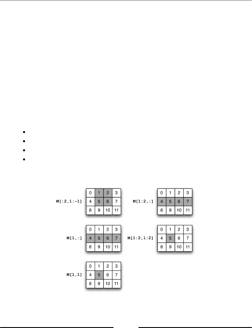
Linear Algebra – Arrays
[ 75 ]
Accessing array entries
Array entries are accessed by indexes. In contrast to vector coefficients two indexes are
needed to access matrix coefficients. These are given in one pair of brackets. This
distinguishes the array syntax from a list of lists. There, two pairs of brackets are needed to
access elements.
M = array([[1., 2.],[3., 4.]])
M[0, 0] # first row, first column: 1.
M[-1, 0] # last row, first column: 3.
Basic array slicing
Slices are similar to those of lists except that there might now be in more than one
dimension:
M[i,:] is a vector filled by the row i of M.
M[:,j] is a vector filled by the column i of M.
M[2:4,:] is a slice of 2:4 on the rows only.
M[2:4,1:4] is a slice on rows and columns.
The result of matrix slicing is given in the following figure (Figure 4.1):
Figure 4.1: The result of matrix slicing
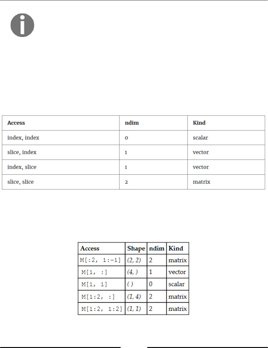
Linear Algebra – Arrays
[ 76 ]
Omitting a dimension
If you omit an index or a slice, NumPy assumes you are taking rows only.
M[3] is a vector that is a view on the third row of M and M[1:3] is a
matrix that is a view on the second and third rows of M.
Changing the elements of a slice affects the entire array:
v = array([1., 2., 3.])
v1 = v[:2] # v1 is array([1., 2.])
v1[0] = 0. # if v1 is changed ...
v # ... v is changed too: array([0., 2., 3.])
General slicing rules are given in the following table (Table 4.3):
Table 4.3: General Slicing Rules
The results of slicing operations for an array M of shape (4, 4) are given in the following table
(Table 4.4):
Table 4.4: Result of slicing operation for an array M of shape (4,4)
Linear Algebra – Arrays
[ 77 ]
Altering an array using slices
You may alter an array using slices or by direct access. The following changes only one
element in a 5 × 3 matrix M:
M[1, 3] = 2.0 # scalar
But we may change one full row of the matrix:
M[2, :] = [1., 2., 3.] # vector
We may also replace a full submatrix:
M[1:3, :] = array([[1., 2., 3.],[-1.,-2., -3.]])
There is a distinction between a column matrix and a vector. The
following assignment with a column matrix returns no error
M[1:4, 2:3] = array([[1.],[0.],[-1.0]])
while the assignment with a vector returns a Value Error
M[1:4, 2:3] = array([1., 0., -1.0]) # error
The general slicing rules are shown in Table 4.2. The matrices and vectors in the preceding
examples must have the right size to fit into matrix M. You may also make use of the
broadcasting rules (for more information, refer to section Broadcasting of Chapter 5,
Advanced Array Concepts) to determine the allowed size of the replacement arrays. If the
replacement array does not have the right shape, a ValueError exception will be raised.
Functions to construct arrays
The usual way to set up an array is via a list. But there are also a couple of convenient
methods for generating special arrays, which are given in the following table (Table 4.5):
Methods Shape Generates
zeros((n,m)) (n,m) Matrix filled with zeros
ones((n,m)) (n,m) Matrix filled with ones
diag(v,k) (n,n) (Sub-, super-) diagonal matrix from a vector v
random.rand(n,m) (n,m) Matrix filled with uniformly distributed random numbers in
(0,1)

Linear Algebra – Arrays
[ 78 ]
arange(n) (n,) First n integers
linspace(a,b,n) (n,) Vector with n equispaced points between a and b
Table 4.5: Commands to create arrays
These commands may take additional arguments. In particular, the commands zeros,
ones, and arange take dtype as an optional argument. The default type is float, except
for arange. There are also methods such as zeros_like and ones_like, which are slight
variants of the preceding ones. For instance, the zeros_like(A) method is equivalent to
zeros(shape(A)).
Here is the identity function, which constructs an identity matrix of a given size:
I = identity(3)
The command is identical to:
I = array([[ 1., 0., 0.],
[ 0., 1., 0.],
[ 0., 0., 1.]])
Accessing and changing the shape
The number of dimensions is what distinguishes a vector from a matrix. The shape is what
distinguishes vectors of different sizes, or matrices of different sizes. In this section, we
examine how to obtain and change the shape of an array.
The shape function
The shape of a matrix is the tuple of its dimensions. The shape of an n × m matrix is the
tuple (n, m). It can be obtained by the shape function:
M = identity(3)
shape(M) # (3, 3)
For a vector, the shape is a singleton containing the length of that vector:
v = array([1., 2., 1., 4.])
shape(v) # (4,) <- singleton (1-tuple)

Linear Algebra – Arrays
[ 79 ]
An alternative is to use the array attribute shape, which gives the same result:
M = array([[1.,2.]])
shape(M) # (1,2)
M.shape # (1,2)
However, the advantage of using shape as a function is that this function may be used on
scalars and lists as well. This may come in handy when code is supposed to work with both
scalars and arrays:
shape(1.) # ()
shape([1,2]) # (2,)
shape([[1,2]]) # (1,2)
Number of dimensions
The number of dimensions of an array is obtained with the function numpy.ndim or using
the array attribute ndarray.ndim :
ndim(A) # 2
A.ndim # 2
Note that the number of dimensions, given by the function ndim, of a tensor T (a vector,
matrix, or higher order tensor) is always equal to the length of its shape:
T = zeros((2,2,3)) # tensor of shape (2,2,3); three dimensions
ndim(T) # 3
len(shape(T)) # 3
Reshape
The method reshape gives a new view of the array, with a new shape, without copying the
data:
v = array([0,1,2,3,4,5])
M = v.reshape(2,3)
shape(M) # returns (2,3)
M[0,0] = 10 # now v[0] is 10
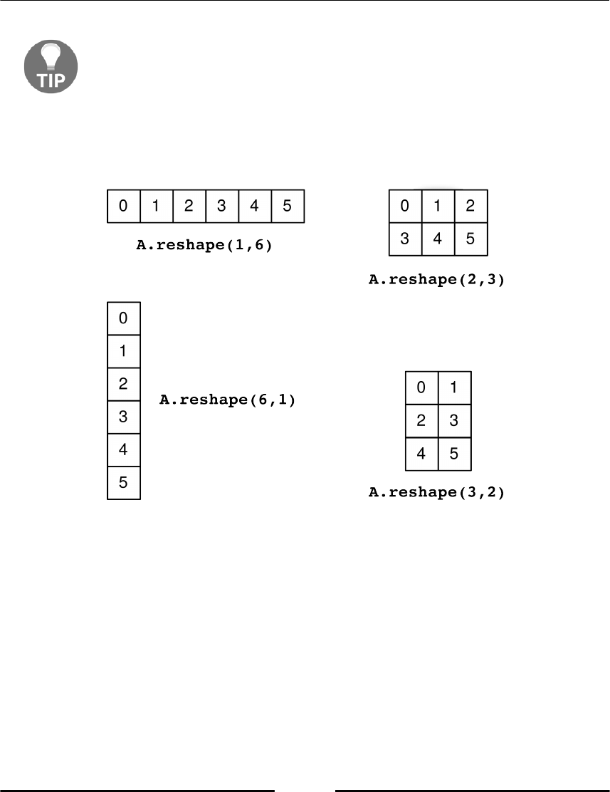
Linear Algebra – Arrays
[ 80 ]
Reshape does not copy
Reshape does not create a new array. It rather gives a new view on the
existing array. In the preceding example, changing one element of M
would automatically result in a change in the corresponding element in v.
When this behavior is not acceptable, you need to copy the data.
The various effects of the reshape method on an array defined by arange(6) are given in
the following figure :
Figure 4.2: The various effects of the reshape method on an array defined by arange(6)
If one tries to reshape an array with a shape that does not multiply to the original shape, an
error is raised:
ValueError: total size of new array must be unchanged.
Linear Algebra – Arrays
[ 81 ]
Sometimes, it is convenient to specify only one shape parameter and let Python determine
the other in such a way that it multiplies to the original shape. This is done by setting the
free shape parameter -1:
v = array([1, 2, 3, 4, 5, 6, 7, 8])
M = v.reshape(2, -1)
shape(M) # returns (2, 4)
M = v.reshape(-1, 2)
shape(M) # returns (4,2 )
M = v.reshape(3,- 1) # returns error
Transpose
A special form of reshaping is transposing. It just switches the two shape elements of the
matrix. The transpose of a matrix A is a matrix B such that:
Which is resolved in the following way:
A = ...
shape(A) # 3,4
B = A.T # A transpose
shape(B) # 4,3
Transpose does not copy
Transposition is very similar to reshaping. In particular, it does not copy
the data either and just returns a view on the same array:
A= array([[ 1., 2.],[ 3., 4.]])
B=A.T
A[1,1]=5.
B[1,1] # 5
Transposing a vector makes no sense since vectors are tensors of one dimension, that is,
functions of one variable. NumPy will, however, comply and return exactly the same object:
v = array([1., 2., 3.])
v.T # exactly the same vector!
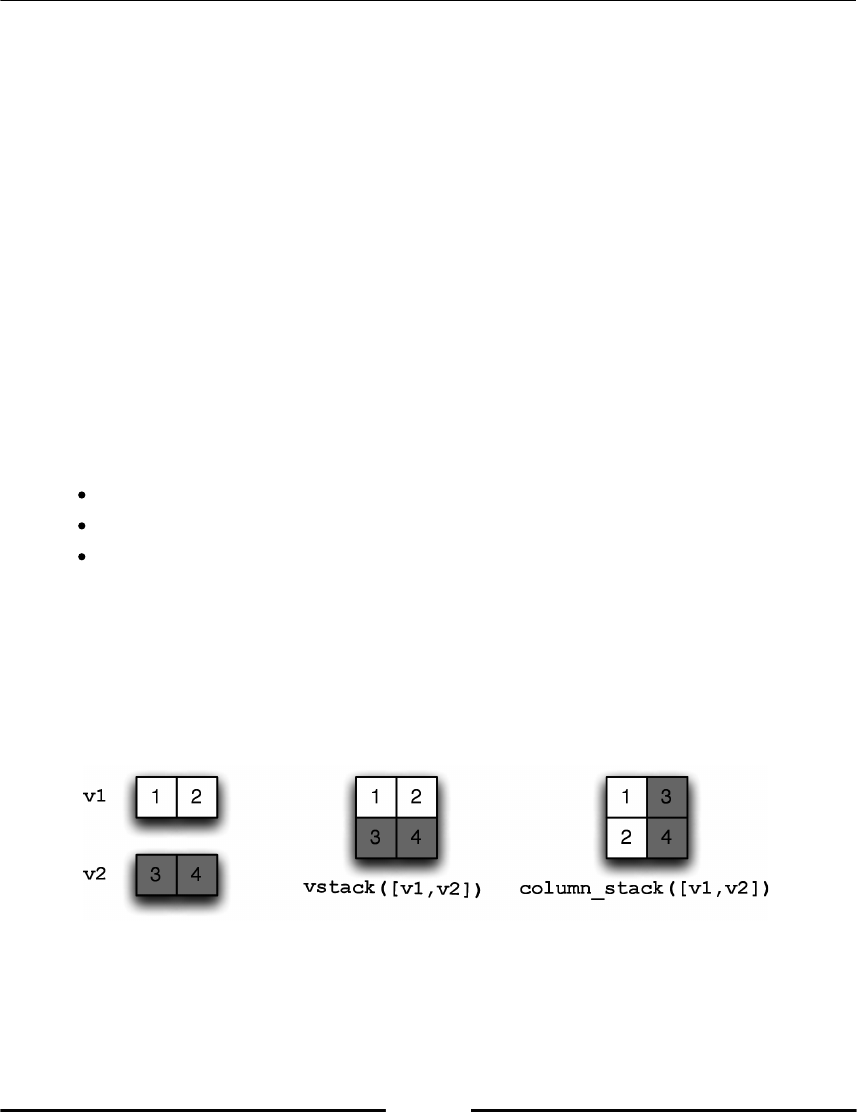
Linear Algebra – Arrays
[ 82 ]
What you have in mind when you want to transpose a vector is probably to create a row or
column matrix. This is done using reshape:
v.reshape(-1, 1) # column matrix containing v
v.reshape(1, -1) # row matrix containing v
Stacking
The universal method to build matrices from a couple of (matching) submatrices is
concatenate. Its syntax is:
concatenate((a1, a2, ...), axis = 0)
This command stacks the submatrices vertically (on top of each other) when axis=0 is
specified. With the axis=1 argument, they are stacked horizontally, and this generalizes
according to arrays with more dimensions. This function is called by several convenient
functions, as follows:
hstack: Used to stack matrices horizontally
vstack: Used to stack matrices vertically
columnstack: Used to stack vectors in columns
Stacking vectors
One may stack vectors row-wise or column-wise using vstack and column_stack, as
illustrated in the following figure:

Linear Algebra – Arrays
[ 83 ]
hstack would produce the concatenation of v1 and v2.
Let us consider the symplectic permutation as an example for vector stacking:
We have a vector of size 2n. We want to perform a symplectic transformation of a vector
with an even number of components, that is, exchange the first half with the second half of
the vector with sign change:
This operation is resolved in Python as follows:
# v is supposed to have an even length.
def symp(v):
n = len(v) // 2 # use the integer division //
return hstack([v[-n:], -v[:n]])
Functions acting on arrays
There are different types of functions acting on arrays. Some act elementwise, and they
return an array of the same shape. Those are called universal functions. Other array
functions return an array of a different shape.
Universal functions
Universal functions are functions that act elementwise on arrays. They thus have an output
array that has the same shape as the input array. These functions allow us to compute the
result of a scalar function on a whole array at once.
Built-in universal functions
A typical example is the cos function (the one provided by NumPy):
cos(pi) # -1
cos(array([[0, pi/2, pi]])) # array([[1, 0, -1]])

Linear Algebra – Arrays
[ 84 ]
Note that universal functions work on arrays in a componentwise manner. This is also true
for operators, such as multiplication or exponent:
2 * array([2, 4]) # array([4, 8])
array([1, 2]) * array([1, 8]) # array([1, 16])
array([1, 2])**2 # array([1, 4])
2**array([1, 2]) # array([1, 4])
array([1, 2])**array([1, 2]) # array([1, 4])
Create universal functions
Your function will automatically be universal if you use only universal functions in it. If,
however, your function uses functions that are not universal, you might get scalar results,
or even an error, when trying to apply them on an array:
def const(x):
return 1
const(array([0, 2])) # returns 1 instead of array([1, 1])
Another example is the following:
def heaviside(x):
if x >= 0:
return 1.
else:
return 0.
heaviside(array([-1, 2])) # error
The expected behaviour would be that the heaviside function applied to a vector [a, b]
would return [heaviside(a), heaviside(b)]. Alas, this does not work because the
function always returns a scalar, no matter the size of the input argument. Besides, using
the function with an array input would raise an exception. The NumPy function
vectorize allows us to quickly solve this problem:
vheaviside = vectorize(heaviside)
vheaviside(array([-1, 2])) # array([0, 1]) as expected

Linear Algebra – Arrays
[ 85 ]
A typical application of this method is its use when plotting a function:
xvals = linspace(-1, 1, 100)
plot(xvals, vectorize(heaviside)(xvals))
axis([-1.5, 1.5, -0.5, 1.5])
The following graph shows the heaviside function:
The vectorize function does not improve performance. It provides only
a convenient way to quickly transform a function, so that it operates
elementwise on list and arrays.
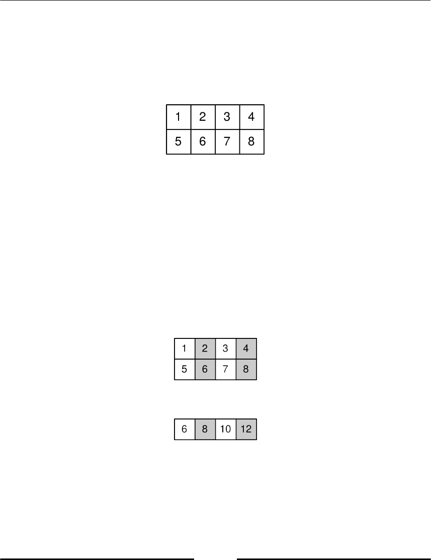
Linear Algebra – Arrays
[ 86 ]
Array functions
There are a number of functions acting on arrays that do not act componentwise. Examples
of such functions are max, min, and sum. These functions may operate on the whole matrix,
row-wise, or column-wise. When no argument is provided, they act on the whole matrix.
Suppose A is the following matrix:
The sum function acting on that matrix returns a scalar:
sum(A) # 36
The command has an optional parameter, axis . It allows us to choose along which axis to
perform the operation. For instance, if the axis is 0, it means that the sum should be
computed along the first axis. The sum along axis 0 of an array of shape (m, n) will be a
vector of length n.
Suppose we compute the sum of A along the axis 0:
sum(A, axis=0) # array([ 6, 8, 10, 12])
This amounts to computing the sum on the columns:
The result is a vector:
Now suppose we compute the sum along the axis 1:
A.sum(axis=1) # array([10, 26])

Linear Algebra – Arrays
[ 87 ]
This amounts to computing the sum on the rows:
The result is a vector:
Linear algebra methods in SciPy
SciPy offers a large range of methods from numerical linear algebra in its scipy.linalg
module. Many of these methods are Python wrapping programs from LAPACK, a collection
of well-approved FORTRAN subroutines used to solve linear equation systems and
eigenvalue problems. Linear algebra methods are the core of any method in scientific
computing, and the fact that SciPy uses wrappers instead of pure Python code makes these
central methods extremely fast. We present in detail here how two linear algebra problems
are solved with SciPy to give you a flavour of this module.
Solving several linear equation systems with LU
Let A be an n × n matrix and b1, b2, …, bk be a sequence of n-vectors. We consider the
problem to find n vectors xi such that:
We assume that the vectors bi are not known simultaneously. In particular, it is quite a
common situation that the ith problem has to be solved before bi+1 becomes available.
LU factorization is a way to organize the classical Gauss elimination method in such a way
that the computation is done in two steps:
A factorization step of the matrix A to get matrices in triangular form
A relatively cheap backward and forward elimination step that works on the bi's
and benefits from the more time-consuming factorization step
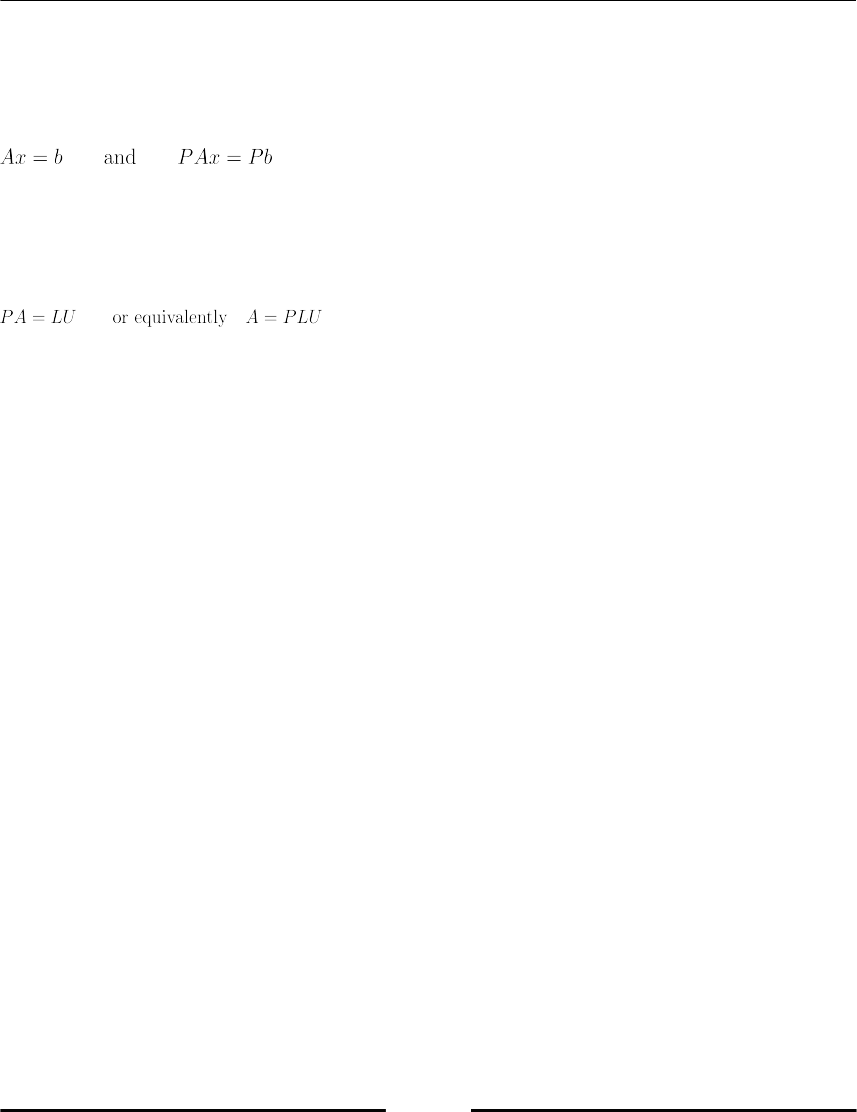
Linear Algebra – Arrays
[ 88 ]
The method also uses the fact that if P is a permutation matrix such that PA is the original
matrix with its rows permuted.
The two systems
have the same solution.
LU factorization finds a permutation matrix P, a lower triangular matrix L, and an upper
triangular matrix U such that:
.
Such a factorization always exists. Furthermore, L can be determined in such a way that Lii =
1. Thus, the essential data from L that has to be stored is Lij with i > j. Consequently, L and U
can be stored together in an n × n array, while the information about the permutation matrix
P just requires an n integer vector – the pivot vector.
In SciPy, there are two methods to compute the LU factorization. The standard one is
scipy.linalg.lu, which returns the three matrices L, U, and P. The other method
islu_factor. That is the method we describe here, because it will be conveniently used
later in combination with lu_solve:
import scipy.linalg as sl
[LU,piv] = sl.lu_factor(A)
Here, the A matrix is factorized and an array with the information about L and U is returned,
together with the pivot vector. With this information, the system can be solved by
performing row interchanges of the vectors bi according to the information stored in the
pivot vector, backward substitution using U, and finally forward substitution using L. This
is bundled in Python, in the lu_solve method. The following code snippet shows how the
system Axi = bi is solved once the LU factorization is performed and its results stored in the
tuple (LU, piv):
import scipy.linalg as sl
xi = sl.lu_solve((LU, piv), bi)
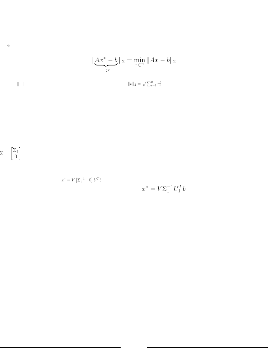
Linear Algebra – Arrays
[ 89 ]
Solving a least square problem with SVD
A linear equation system Ax = b, with A being an m × n matrix and m > n, is called an
overdetermined linear system. In general it has no classical solution and one seeks a vector
x* ℝn with the property:
Here, denotes the Euclidean vector norm .
This problem is called a least square problem. A stable method to solve it is based on
factorizing A = UΣVT, with U being a m × m orthogonal matrix, V a n × n orthogonal matrix,
and Σ = (σij) an m × n matrix with the property σij = 0 for all i ≠j. This factorization is called a
singular value decomposition (SVD).
We write,
with a diagonal n × n matrix Σ1. If we assume that A has full rank, then Σ1 is invertible and
it can be shown that, . If we split U = [U1 U2] with U1 being an m × n submatrix,
then the preceding equation can be simplified to .
SciPy provides a function called svd, which we use to solve this task:
import scipy.linalg as sl
[U1, Sigma_1, VT] = sl.svd(A, full_matrices = False,
compute_uv = True)
xast = dot(VT.T, dot(U1.T, b) / Sigma_1)
r = dot(A, xast) - b # computes the residual
nr = sl.norm(r, 2) # computes the Euclidean norm of r
Linear Algebra – Arrays
[ 90 ]
The keyword full_matrices says that only the portion U1 of U needs to be computed. As
one often uses svd to compute only singular values, σii, we have to explicitly demand the
computation of U and V by using the keyword compute_uv. The SciPy function
scipy.linalg.lstsq solves the least square problem similarly by using a singular value
decomposition.
More methods
In the examples so far, you met a couple of methods for computational tasks in linear
algebra, for example, solve. Most common methods are available after the
command import scipy.linalg as sl is executed. We refer to their documentation for
further reference. Some linear algebra functions of the scipy.linalg module are given in
the following table (Table 4.6):
Methods Description (matrix methods)
sl.det Determinant of a matrix
sl.eig Eigenvalues and eigenvectors of a matrix
sl.inv Matrix inverse
sl.pinv Matrix pseudoinverse
sl.norm Matrix or vector norm
sl.svd Singular value decomposition
sl.lu LU decomposition
sl.qr QR decomposition
sl.cholesky Cholesky decomposition
sl.solve Solution of a general or symmetric linear system: Ax = b
sl.solve.banded The same for banded matrices
sl.lstsq Least squares solution
Table 4.6: Linear algebra functions of the scipy.linalg module
Execute import scipy.linalg as sl first.
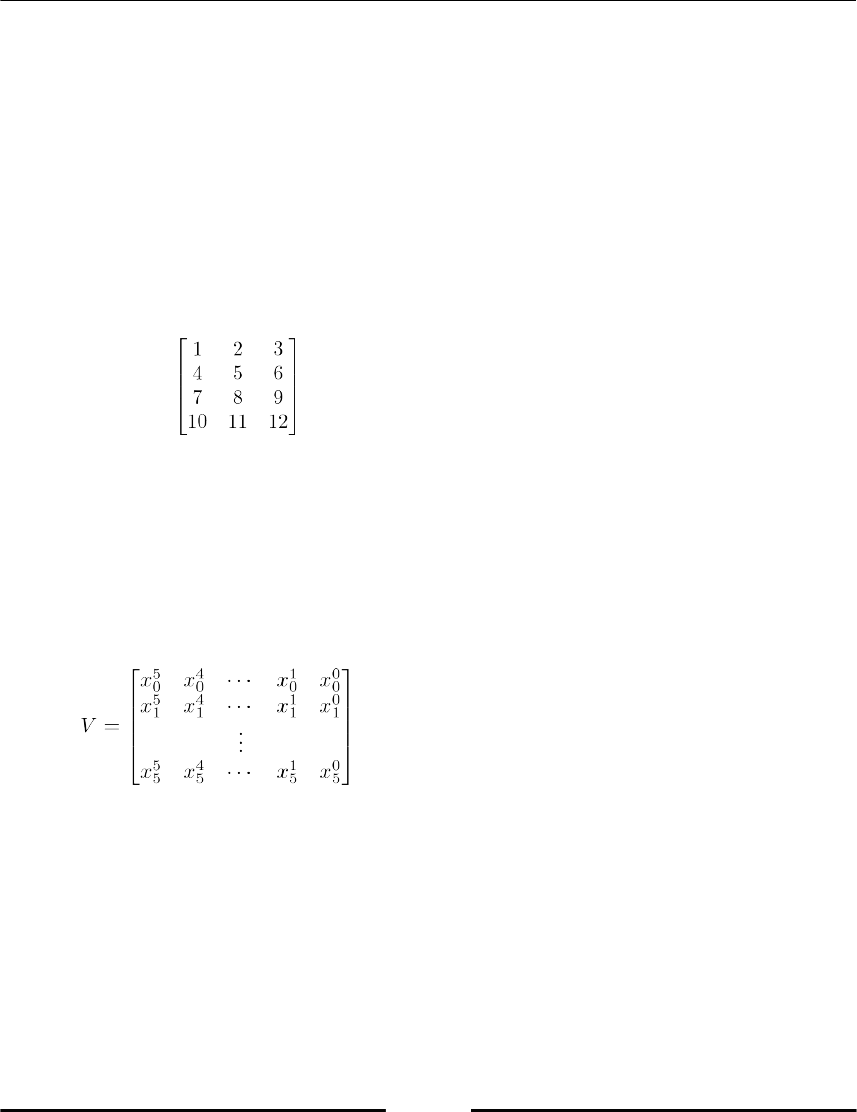
Linear Algebra – Arrays
[ 91 ]
Summary
In this chapter, we worked with the most important objects in linear algebra – vectors and
matrices. For this, we learned how to define arrays and we met important array methods. A
smaller section demonstrated how to use modules from scipy.linalg to solve central
tasks in linear algebra.
Exercises
Ex. 1 → Consider a 4 × 3 matrix M:
Construct this matrix in Python using the function array .1.
Construct the same matrix using the function arange followed by a suitable2.
reshape.
What is the result of the expression M[2,:] ? What is the result of the similar3.
expression M[2:]?
Ex. 2 → Given a vector x, construct in Python the following matrix:
Linear Algebra – Arrays
[ 92 ]
Here, xi are the components of the vector x (numbered from zero). Given a vector y, solve in
Python the linear equation system Va = y. Let the components of a be denoted by ai, i = 0, …,
5. Write a function poly, which has a and z as input and which computes the polynomial:
Plot this polynomial and depict in the same plot the points (xi, yi) as small stars. Try your
code with the vectors:
x = (0.0, 0.5, 1.o, 1.5, 2.0, 2.5)
y = (-2.0, 0.5, -2.0, 1.0, -0.5, 1.0)
Ex. 3 → The matrix V in Ex. 2 is called a Vandermonde matrix. It can be set up in Python
directly by the command vander. Evaluating a polynomial defined by a coefficient vector
can be done with the Python command polyval. Repeat Ex. 2 by using these commands.
Ex. 4 → Let u be a one dimensional array. Construct another array ξ with values ξi = (u1 + ui+1
+ ui+2)/3. In statistics, this array is called the moving average of u. In approximation theory, it
plays the role as the Greville abscissae of cubic splines. Try to avoid the use of for loops in
your script.
Ex. 5 →
Construct from the matrix V given in Ex. 2 a matrix A by deleting V's first column.1.
Form the matrix B = (AT A)-1 AT.2.
Compute c = B y with y from Ex. 2.3.
Use c and polyval to plot the polynomial defined by c. Plot in the same picture4.
again the points (xi, yi).
Ex. 6 → Ex. 5 describes the least square method. Repeat that exercise but use SciPy's
scipy.linalg.lstsq method instead.
Linear Algebra – Arrays
[ 93 ]
Ex. 7 → Let v be a vector written in its coordinate form as a 3 × 1 matrix
[1 -1 1]T. Construct the projection matrices:
.
Show experimentally that v is an eigenvector for both matrices P and Q. What are the
corresponding eigenvalues?
Ex. 8 → In numerical linear algebra the m × m matrix A with the property
is used as an example for an extreme growth-factor, when performing LU factorization.
Set up this matrix in Python for various m, compute its LU factorization using the
command scipy.linalg.lu and derive experimentally a statement about the growth
factor
in relation to m.
5
Advanced Array Concepts
In this chapter, we will explain some more advanced aspects of arrays. First, we will cover
the notion of an array view, followed by Boolean arrays and how to compare arrays. We
briefly describe indexing and vectorization, explain sparse arrays, and some special topics
such as broadcasting.
Array views and copies
In order to control precisely how memory is used, NumPy offers the concept of view of an
array. Views are smaller arrays that share the same data as a larger array. This works just
like a reference to one single object (refer to section Basic Types in Chapter 1, Getting
Started).
Array views
The simplest example of a view is given by a slice of an array:
M = array([[1.,2.],[3.,4.]])
v = M[0,:] # first row of M
The preceding slice is a view of M. It shares the same data as M. Modifying v will modify M as
well:
v[-1] = 0.
v # array([[1.,0.]])
M # array([[1.,0.],[3.,4.]]) # M is modified as well

Advanced Array Concepts
[ 95 ]
It is possible to access the object that owns the data using the array attribute base:
v.base # array([[1.,0.],[3.,4.]])
v.base is M # True
If an array owns its data, the attribute base is none :
M.base # None
Slices as views
There are precise rules on which slices will return views and which ones will return copies.
Only basic slices (mainly index expressions with :) return views, whereas any advanced
selections (such as slicing with a Boolean) will return a copy of the data. For instance, it is
possible to create new matrices by indexing with lists (or arrays):
a = arange(4) # array([0.,1.,2.,3.])
b = a[[2,3]] # the index is a list [2,3]
b # array([2.,3.])
b.base is None # True, the data was copied
c = a[1:3]
c.base is None # False, this is just a view
In the preceding example, the array b is not a view, whereas the array c, obtained with a
simpler slice, is a view.
There is an especially simple slice of an array that returns a view of the whole array:
N = M[:] # this is a view of the whole array M
Transpose and reshape as views
Some other important operations return views. For instance, transpose returns a view:
M = random.random_sample((3,3))
N = M.T
N.base is M # True
The same applies for all reshaping operations:
v = arange(10)
C = v.reshape(-1,1) # column matrix
C.base is v # True

Advanced Array Concepts
[ 96 ]
Array copy
Sometimes it is necessary to explicitly request that the data be copied. This is simply
achieved with the NumPy function called array:
M = array([[1.,2.],[3.,4.]])
N = array(M.T) # copy of M.T
We may verify that the data has indeed been copied:
N.base is None # True
Comparing arrays
Comparing two arrays is not as simple as it may seem. Consider the following code, which
is intended to check whether two matrices are close to each other:
A = array([0.,0.])
B = array([0.,0.])
if abs(B-A) < 1e-10: # an exception is raised here
print("The two arrays are close enough")
This code raises the exception when the if statement is executed:
ValueError: The truth value of an array with more than one element is
ambiguous. Use a.any() or a.all()
In this section, we explain why this is so and how to remedy this state of affairs.
Boolean arrays
Boolean arrays are useful for advanced array indexing (refer to section Indexing with Boolean
arrays). A Boolean array is simply an array for which the entries have the type bool:
A = array([True,False]) # Boolean array
A.dtype # dtype('bool')

Advanced Array Concepts
[ 97 ]
Any comparison operator acting on arrays will create a Boolean array instead of a simple
Boolean:
M = array([[2, 3],
[1, 4]])
M > 2 # array([[False, True],
# [False, True]])
M == 0 # array([[False, False],
# [False, False]])
N = array([[2, 3],
[0, 0]])
M == N # array([[True, True],
# [False, False]])
...
Note that because array comparison creates Boolean arrays, one cannot use array
comparison directly in conditional statements, for example, if statements. the solution is to
use the methods all and any:
A = array([[1,2],[3,4]])
B = array([[1,2],[3,3]])
A == B # creates array([[True, True], [True, False]])
(A == B).all() # False
(A != B).any() # True
if (abs(B-A) < 1e-10).all():
print("The two arrays are close enough")
Checking for equality
Checking for equality of two float arrays is not straight forward, because two floats may be
very close without being equal. In NumPy, it is possible to check for equality with
allclose. This function checks for equality of two arrays up to a given precision:
data = random.rand(2)*1e-3
small_error = random.rand(2)*1e-16
data == data + small_error # False
allclose(data, data + small_error, rtol=1.e-5, atol=1.e-8) # True
The tolerance is given in terms of a relative tolerance bound, rtol, and an absolute error
bound, atol. The command allclose is a short form of: (abs(A-B) <
atol+rtol*abs(B)).all().
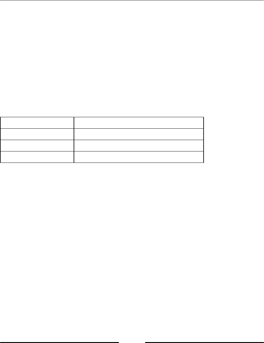
Advanced Array Concepts
[ 98 ]
Note that allclose can be also applied to scalars:
data = 1e-3
error = 1e-16
data == data + error # False
allclose(data, data + error, rtol=1.e-5, atol=1.e-8) #True
Boolean operations on arrays
You cannot use and, or, and not on Boolean arrays. Indeed, those operators force the
casting from array to Boolean, which is not permitted. Instead, we can use the operators
given in the following table (Table 5.1) for componentwise logical operations on Boolean
arrays:
Logic operator Replacement for Boolean arrays
A and B A & B
A or B A | B
not A ~ A
Table 5.1 Logical operators and, or and not do not work with arrays.
A = array([True, True, False, False])
B = array([True, False, True, False])
A and B # error!
A & B # array([True, False, False, False])
A | B # array([True, True, True, False])
~A # array([False, False, True, True])
Here is an example usage of logical operators with Boolean arrays:
Suppose that we have a sequence of data that is marred with some measurement error.
Suppose further that we run a regression and it gives us a deviation for each value. We wish
to obtain all the exceptional values and all the values with little deviation that are lower
than a given threshold:
data = linspace(1,100,100) # data
deviation = random.normal(size=100) # the deviations
#don't forget the parentheses in next statement!
exceptional = data[(deviation<-0.5)|(deviation>0.5)]
exceptional = data[abs(deviation)>0.5] # same result
small = data[(abs(deviation)<0.1)&(data<5.)] # small deviation and data

Advanced Array Concepts
[ 99 ]
Array indexing
We have already seen that one may index arrays by combinations of slices and integers, this
is the basic slicing technique. There are, however, many more possibilities, which allow for
a variety of ways to access and modify array elements.
Indexing with Boolean arrays
It is often useful to access and modify only parts of an array, depending on its value. For
instance, one might want to access all the positive elements of an array. This turns out to be
possible using Boolean arrays, which act like masks to select only some elements of an
array. The result of such an indexing is always a vector. For instance, consider the following
example:
B = array([[True, False],
[False, True]])
M = array([[2, 3],
[1, 4]])
M[B] # array([2,4]), a vector
In fact, the M[B] call is equivalent to M.flatten()[B]. One may then replace the resulting
vector by another vector. For instance, one may replace all the elements by zero (refer to
section Broadcasting for more information):
M[B] = 0
M # [[0, 3], [1, 0]]
Or one may replace all the selected values by others:
M[B] = 10, 20
M # [[10, 3], [1, 20]]
By combining the creation of Boolean arrays (M > 2), smart indexing (indexing with
Boolean array), and broadcasting, one may use the following elegant syntax:
M[M>2] = 0 # all the elements > 2 are replaced by 0
The expression broadcasting here refers to the tacit conversion of the scalar 0 to a vector of
an appropriate shape.
Advanced Array Concepts
[ 100 ]
Using where
The command where gives a useful construct that can take a Boolean array as a condition
and either return the indexes of the array elements satisfying the condition or return
different values depending on the values in the Boolean array.
The basic structure is:
where(condition, a, b)
This will return values from a when the condition is True and values from b when it is
False.
For instances consider, a Heaviside function:
The following code implements a Heaviside function:
def H(x):
return where(x < 0, 0, 1)
x = linspace(-1,1,11) # [-1. -0.8 -0.6 -0.4 -0.2 0. 0.2 0.4 0.6 0.8 1. ]
print(H(x)) # [0 0 0 0 0 1 1 1 1 1 1]
The second and third arguments can be either arrays of the same size as the condition (the
Boolean array) or scalars. We give two more example to demonstrated how to manipulate
elements from an array or a scalar depending on a condition:
x = linspace(-4,4,5)
# [-4. -2. 0. 2. 4.]
print(where(x > 0, sqrt(x), 0))
# [ 0.+0.j 0.+0.j 0.+0.j 1.41421356+0.j 2.+0.j ]
print(where(x > 0, 1, -1)) # [-1 -1 -1 1 1]
If the second and third arguments are omitted, then a tuple containing the indexes of the
elements satisfying the condition is returned.

Advanced Array Concepts
[ 101 ]
For example consider the use of where with only one argument in the following code:
a = arange(9)
b = a.reshape((3,3))
print(where(a > 5)) # (array([6, 7, 8]),)
print(where(b > 5)) # (array([2, 2, 2]), array([0, 1, 2]))
Performance and Vectorization
When it comes to performance of your Python code, it often boils down to the difference
between interpreted code and compiled code. Python is an interpreted programming
language and basic Python code is executed directly without any intermediate compilation
to machine code. With a compiled language, the code needs to be translated to machine
instructions before execution.
The benefits of an interpreted language are many but interpreted code cannot compete with
compiled code for speed. To make your code faster, you can write some parts in a compiled
language like FORTRAN, C, or C++. This is what NumPy and SciPy do.
For this reason, it is best to use functions in NumPy and SciPy over interpreted versions
whenever possible. NumPy array operations such as matrix multiplication, matrix-vector
multiplication, matrix factorization, scalar products, and so on are much faster than any
pure Python equivalent. Consider the simple case of scalar products. The scalar product is
much slower than the compiled NumPy function, dot(a,b) (more than 100 times slower
for arrays with about 100 elements):
def my_prod(a,b):
val = 0
for aa,bb in zip(a,b):
val += aa*bb
return val
Measuring the speed of your functions is an important aspect of scientific computing. Refer
to section Measuring execution time in Chapter 13, Testing, for details on measuring
execution times.

Advanced Array Concepts
[ 102 ]
Vectorization
To improve performance, one has to vectorize the code often. Replacing for loops and
other slower parts of the code with NumPy slicing, operations, and functions can give
significant improvements. For example, the simple addition of a scalar to a vector by
iterating over the elements is very slow:
for i in range(len(v)):
w[i] = v[i] + 5
where using NumPy's addition is much faster:
w = v + 5
Using NumPy slicing can also give significant speed improvements over iterating with for
loops. To demonstrate this let us consider forming the average of neighbors in a two-
dimensional array:
def my_avg(A):
m,n = A.shape
B = A.copy()
for i in range(1,m-1):
for j in range(1,n-1):
B[i,j] = (A[i-1,j] + A[i+1,j] + A[i,j-1] + A[i,j+1])/4
return B
def slicing_avg(A):
A[1:-1,1:-1] = (A[:-2,1:-1] + A[2:,1:-1] +
A[1:-1,:-2] + A[1:-1,2:])/4
return A
These functions both assign each element the average of its four neighbors. The second
version, using slicing, is much faster.
Besides replacing for loops and other slower constructions with NumPy functions, there is
a useful function called vectorize, refer to section Functions acting on arrays in Chapter 4,
Linear Algebra – Arrays. This will take a function and create a vectorized version that applies
the function on all elements of an array using functions wherever possible.

Advanced Array Concepts
[ 103 ]
Consider the following example for vectorizing a function:
def my_func(x):
y = x**3 - 2*x + 5
if y>0.5:
return y-0.5
else:
return 0
Applying this by iterating over an array is very slow:
for i in range(len(v)):
v[i] = my_func(v[i])
Instead, use vectorize to create a new function, like this:
my_vecfunc = vectorize(my_func)
This function can then be applied to the array directly:
v = my_vecfunc(v)
The vectorized option is much faster (around 10 times faster with arrays of length 100).
Broadcasting
Broadcasting in NumPy denotes the ability to guess a common, compatible shape between
two arrays. For instance, when adding a vector (one-dimensional array) and a scalar (zero-
dimensional array), the scalar is extended to a vector, in order to allow for the addition. The
general mechanism is called broadcasting. We will first review that mechanism from a
mathematical point of view, and then proceed to give the precise rules for broadcasting in
NumPy.
Mathematical view
Broadcasting is often performed in mathematics, mainly implicitly. Examples are
expressions such as f(x) + C or f(x) + g(y). We'll give an explicit description of that technique
in this section.
Advanced Array Concepts
[ 104 ]
We have in mind the very close relationship between functions and NumPy arrays, as
described in section Mathematical preliminaries of Chapter 4, Linear Algebra – Arrays.
Constant functions
One of the most common examples of broadcasting is the addition of a function and a
constant; if C is a scalar, one often writes:
This is an abuse of notation since one should not be able to add functions and constants.
Constants are however implicitly broadcast to functions. The broadcast version of the
constant C is the function defined by:
Now it makes sense to add two functions together:
We are not being pedantic for the sake of it, but because a similar situation may arise for
arrays, as in the following code:
vector = arange(4) # array([0.,1.,2.,3.])
vector + 1. # array([1.,2.,3.,4.])
In this example, everything happens as if the scalar 1. had been converted to an array of
the same length as vector, that is, array([1.,1.,1.,1.]), and then added to vector.
This example is exceedingly simple, so we proceed to show less obvious situations.
Advanced Array Concepts
[ 105 ]
Functions of several variables
A more intricate example of broadcasting arises when building functions of several
variables. Suppose, for instance, that we were given two functions of one variable, f and g,
and that we want to construct a new function F according to the formula:
This is clearly a valid mathematical definition. We would like to express this definition as
the sum of two functions in two variables defined as
and now we may simply write:
The situation is similar to that arising when adding a column matrix and a row matrix:
C = arange(2).reshape(-1,1) # column
R = arange(2).reshape(1,-1) # row
C + R # valid addition: array([[0.,1.],[1.,2.]])
This is especially useful when sampling functions of two variables, as shown in section
Typical examples.
General mechanism
We have seen how to add a function and a scalar and how to build a function of two
variables from two functions of one variable. Let us now focus on the general mechanism
that makes this possible. The general mechanism consists of two steps: reshaping and
extending.

Advanced Array Concepts
[ 106 ]
First, the function g is reshaped to a function that takes two arguments. One of these
arguments is a dummy argument, which we take to be zero, as a convention:
Mathematically, the domain of definition of is now Then the function f is reshaped
in a way similar to:
Now both and take two arguments, although one of them is always zero. We proceed to
the next step, extending. It is the same step that converted a constant into a constant
function (refer to the constant function example).
The function is extended to:
The function is extended to:
Now the function of two variables F, which was sloppily defined by F(x,y) = f(x) + g(y), may
be defined without reference to its arguments:
For example, let us describe the preceding mechanism for constants. A constant is a scalar,
that is, a function of zero arguments. The reshaping step is thus to define the function of one
(empty) variable:
Now the extension step proceeds simply by:
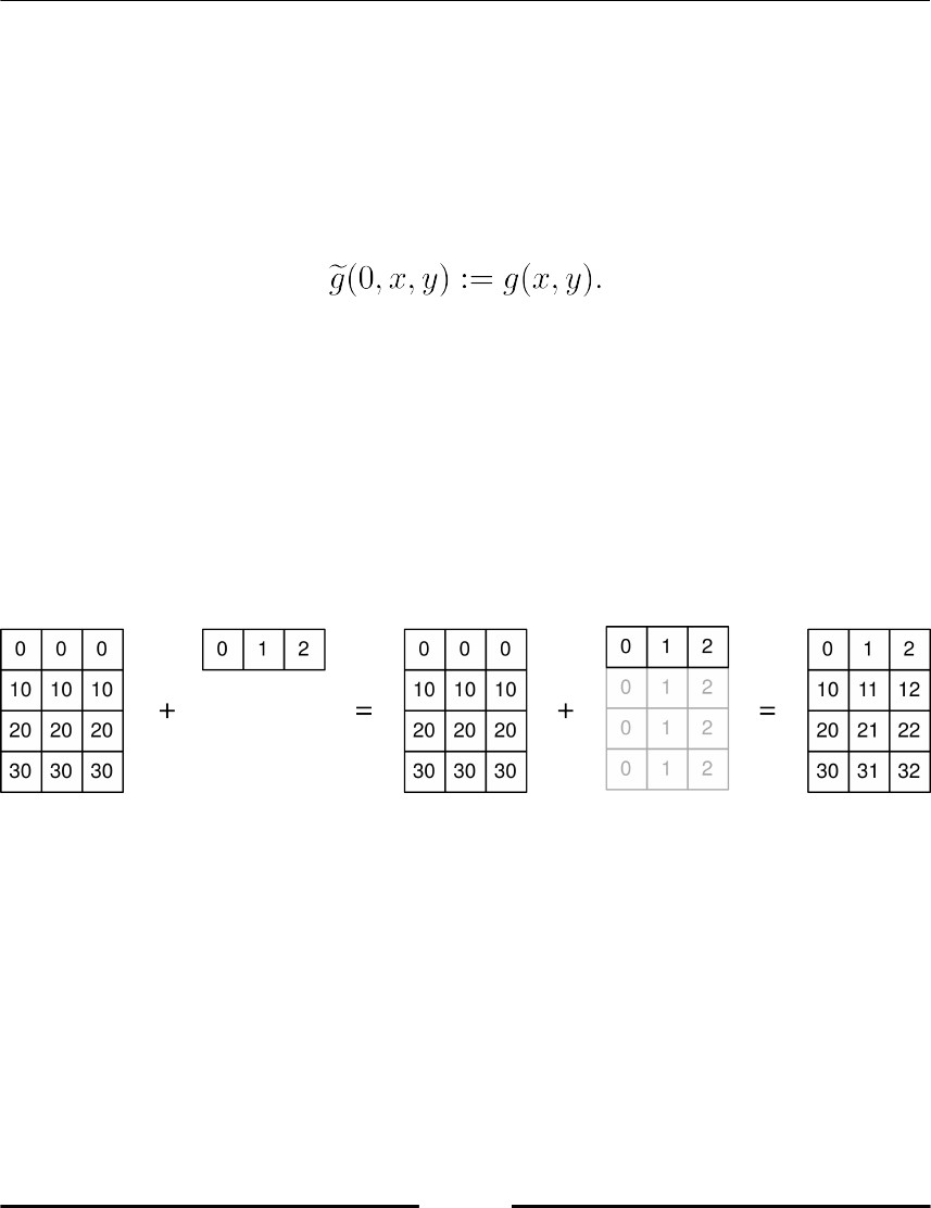
Advanced Array Concepts
[ 107 ]
Conventions
The last ingredient is the convention on how to add the extra arguments to a function, that
is, how the reshaping is automatically performed. By convention, a function is
automatically reshaped by adding zeros on the left.
For example, if a function g of two arguments has to be reshaped to three arguments, the
new function would be defined by:
Broadcasting arrays
We now repeat the observation that arrays are merely functions of several variables (refer to
section Mathematical preliminaries in Chapter 4, Linear Algebra – Arrays). Array broadcasting
thus follows exactly the same procedure as explained above for mathematical functions.
Broadcasting is done automatically in NumPy.
In the following figure (Figure 5.1), we show what happens when adding a matrix of shape
(4, 3) to a matrix of size (1, 3). The second matrix is of the shape (4, 3):
Figure 5.1: Broadcasting between a matrix and a vector.
The broadcasting problem
When NumPy is given two arrays with different shapes, and is asked to perform an
operation that would require the two shapes to be the same, both arrays are broadcast to a
common shape.
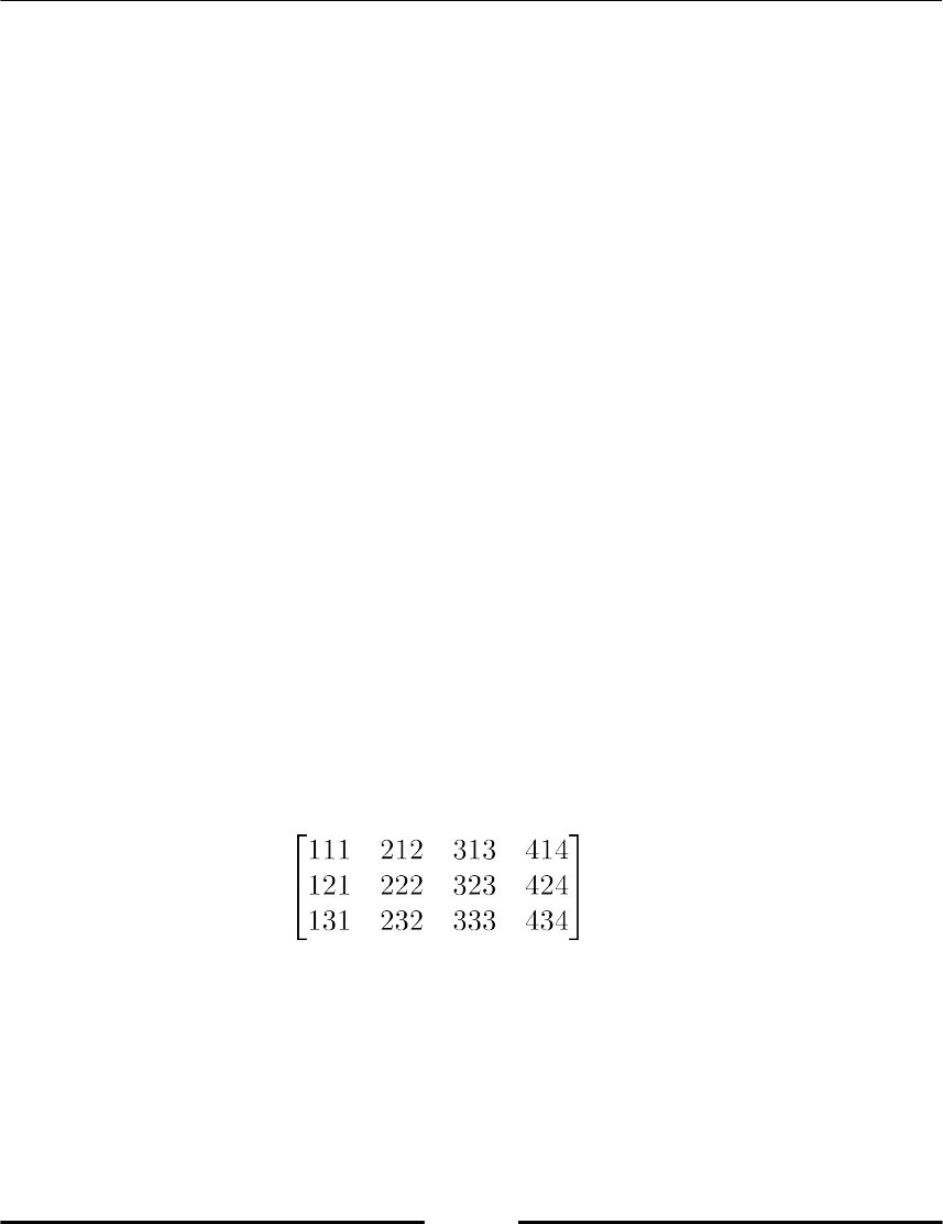
Advanced Array Concepts
[ 108 ]
Suppose the two arrays have shapes s1 and s2. This broadcasting is performed in two steps:
If the shape s1 is shorter than the shape s2 then ones are added on the left of the1.
shape s1. This is a reshaping.
When the shapes have the same length, the array is extended to match the shape2.
s2 (if possible).
Suppose we want to add a vector of shape (3, ) to a matrix of shape (4, 3). The vector needs
be broadcast. The first operation is a reshaping; the shape of the vector is converted from (3,
) to (1, 3). The second operation is an extension; the shape is converted from (1, 3) to (4, 3).
For instance, suppose a vector of size n is to be broadcast to the shape (m, n):
v is automatically reshaped to (1, n).1.
v is extended to (m, n).2.
To demonstrate this we consider a matrix defined by:
M = array([[11, 12, 13, 14],
[21, 22, 23, 24],
[31, 32, 33, 34]])
and vector given by:
v = array([100, 200, 300, 400])
Now we may add M and v directly:
M + v # works directly
The result is this matrix:
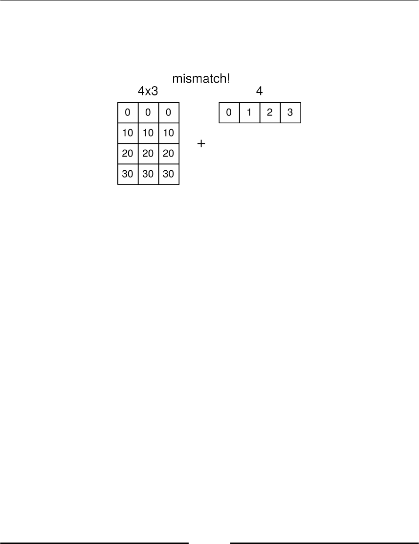
Advanced Array Concepts
[ 109 ]
Shape mismatch
It is not possible to automatically broadcast a vector v of length n to the shape (n,m). This
is illustrated in the following figure:
The broadcasting will fail, because the shape (n,) may not be automatically broadcast to
the shape (m, n). The solution is to manually reshape v to the shape (n,1). The
broadcasting will now work as usual (by extension only):
M + v.reshape(-1,1)
Here is another example, define a matrix by:
M = array([[11, 12, 13, 14],
[21, 22, 23, 24],
[31, 32, 33, 34]])
and a vector by:
v = array([100, 200, 300])
Now automatic broadcasting will fail, because automatic reshaping does not work:
M + v # shape mismatch error
The solution is thus to take care of the reshaping manually. What we want in that case is to
add 1 on the right, that is, transform the vector into a column matrix. The broadcasting then
works directly:
M + v.reshape(-1,1)
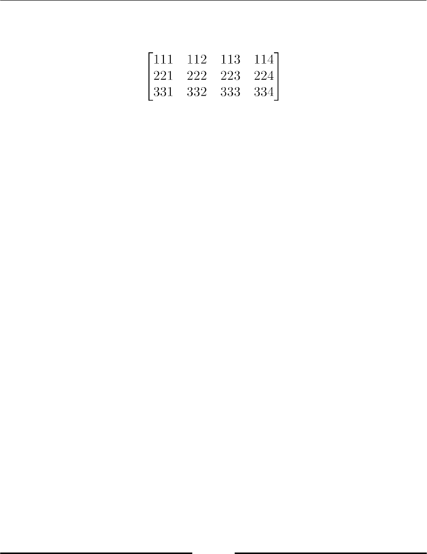
Advanced Array Concepts
[ 110 ]
For the shape parameter -1, refer to section Accessing and changing the shape of Chapter 4,
Linear Algebra - Arrays. The result is this matrix:
Typical examples
Let us examine some typical examples where broadcasting may come in handy.
Rescale rows
Suppose M is an n × m matrix, and we want to multiply each row by a coefficient. The
coefficients are stored in a vector coeff with n components. In that case, automatic
reshaping will not work, and we have to execute:
rescaled = M*coeff.reshape(-1,1)
Rescale columns
The setup is the same here, but we would like to rescale each column with a coefficient
stored in a vector coeff of length m. In this case, automatic reshaping will work:
rescaled = M*coeff
Obviously, we may also do the reshaping manually and achieve the same result with:
rescaled = M*coeff.reshape(1,-1)
Functions of two variables
Suppose u and v are vectors and we want to form the matrix W with elements wij = ui + vj.
This would correspond to the function F(x, y) = x + y. The matrix W is merely defined by:
W=u.reshape(-1,1) + v
Advanced Array Concepts
[ 111 ]
If the vectors u and v are [0, 1] and [0, 1, 2] respectively, the result is:
More generally, suppose that we want to sample the function w(x, y) := cos(x) + sin(2y).
Supposing that the vectors x and y are defined, the matrix w of sampled values is obtained
by:
w = cos(x).reshape(-1,1) + sin(2*y)
Note that this is very frequently used in combination with ogrid. The vectors obtained
from ogrid are already conveniently shaped for broadcasting. This allows for the following
elegant sampling of the function cos(x) + sin(2y):
x,y = ogrid[0:1:3j,0:1:3j]
# x,y are vectors with the contents of linspace(0,1,3)
w = cos(x) + sin(2*y)
The syntax of ogrid needs some explanation. First, ogrid is no function. It is an instance of
a class with a __getitem__ method (refer to section Attributes in Chapter 8, Classes). That
is why it is used with brackets instead of parentheses.
The two commands are equivalent:
x,y = ogrid[0:1:3j, 0:1:3j]
x,y = ogrid.__getitem__((slice(0, 1, 3j),slice(0, 1, 3j)))
The stride parameter in the preceding example is a complex number. This is to indicate that
it is the number of steps instead of the step size. The rules for the stride parameter might be
confusing at first glance:
If the stride is a real number, then it defines the size of the steps between start
and stop and stop is not included in the list.
If the stride is a complex number s, then the integer part of s.imag defines the
number of steps between start and stop and stop is included in the list.

Advanced Array Concepts
[ 112 ]
Another example for the output of ogrid is a tuple with two arrays, which can be used for
broadcasting:
x,y = ogrid[0:1:3j, 0:1:3j]
gives:
array([[ 0. ],
[ 0.5],
[ 1. ]])
array([[ 0. , 0.5, 1. ]])
which is equivalent to:
x,y = ogrid[0:1.5:.5, 0:1.5:.5]
Sparse matrices
Matrices with a small number of nonzero entries are called sparse matrices. Sparse matrices
occur, for example, in scientific computing when describing discrete differential operators
in the context of numerically solving partial differential equations.
Sparse matrices often have large dimensions, sometimes so large that the entire matrix
(with zero entries) would not even fit in the available memory. This is one motivation for a
special type for sparse matrices. Another motivation is better performance of operations
where zero matrix entries can be avoided.
There are only a very limited number of algorithms for general, unstructured sparse
matrices in linear algebra. Most of them are iterative in nature and based on efficient
implementations of matrix-vector multiplication for sparse matrices.
Examples for sparse matrices are diagonal or banded matrices. The simple pattern of these
matrices allows straightforward storing strategies; the principal diagonal and the sub- and
super-diagonals are stored in 1D arrays. Conversion from a sparse representation to the
classical array type and vice-versa can be done by the command diag.
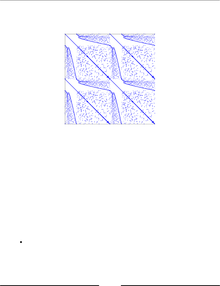
Advanced Array Concepts
[ 113 ]
In general, there is not such a simple structure and the description of sparse matrices
requires special techniques and standards. Here we present a row and a column oriented
type for sparse matrices, both available through the module scipy.sparse .
Figure 5.2: A stiffness matrix from a finite element model of an elastic plate. The pixels denote nonzero entries
in the 1250 × 1250 matrix
Sparse matrix formats
The scipy.sparse module provides many different storing formats from sparse matrices.
We describe here only the most important ones: CSR, CSC, and LIL. The LIL format should
be used for generating and altering sparse matrices; CSR and CSC are efficient formats for
matrix-matrix and matrix-vector operations.
Compressed sparse row
The compressed sparse row format (CSR) uses three arrays: data, indptr, and indices:
The 1D array data stores all the nonzero values in order. It has as many elements
as there are nonzero elements, often denoted by the variable nnz.
Advanced Array Concepts
[ 114 ]
The 1D array indptr contains integers such that indptr[i] is the index of the
element in data, which is the first nonzero element of row i. If the entire row i is
zero, then indptr[i]==indptr[i+1]. If the original matrix has m rows, then
len(indptr)==m+1.
The 1D array indices contains the column index information in such a way that
indices[indptr[i]:indptr[i+1]] is an integer array with the column
indexes of the nonzero elements in row i. Obviously,
len(indices)==len(data)==nnz.
Let's see an example:
The CSR format of the matrix:
is given by the three arrays:
data = (1. 2. 3. 4.)
indptr = (0 2 2 3 5)
indices = (0 2 0 0 3)
The module scipy.sparse provides a type, csr_matrix, with a constructor, which can be
used in the following ways:
With a 2D array as argument
With a matrix in one of the other sparse formats in scipy.sparse
With a shape argument, (m,n), to generate a zero matrix in CSR format
By a 1D array for the data and an integer array ij with the shape
(2,len(data)) such that ij[0,k] is the row index and ij[1,k] is the column
index of data[k] of the matrix
The three arguments, data, indptr, and indices, can be given to the
constructor directly
The first two options are there for conversion purposes while the last two directly define the
sparse matrix.

Advanced Array Concepts
[ 115 ]
Consider the above example in python look like:
import scipy.sparse as sp
A = array([[1,0,2,0],[0,0,0,0],[3.,0.,0.,0.],[1.,0.,0.,4.]])
AS = sp.csr_matrix(A)
Among others, the following attributes are provided:
AS.data # returns array([ 1., 2., 3., 1., 4.])
AS.indptr # returns array([0, 2, 2, 3, 5])
AS.indices # returns array([0, 2, 0, 0, 3])
AS.nnz # returns 5
Compressed Sparse Column
The CSR format has a column oriented twin – the compressed sparse column (CSC) format.
The only difference in it compared to the CSR format is the definition of the indptr and
indices arrays, which are now column-related. The type for the CSC format is
csc_matrix and its use corresponds to csr_matrix, explained previously in this section.
Continuing the same example in CSC format:
import scipy.sparse as sp
A = array([[1,0,2,0],[0,0,0,0],[3.,0.,0.,0.],[1.,0.,0.,4.]])
AS = sp.csc_matrix(A)
AS.data # returns array([ 1., 3., 1., 2., 4.])
AS.indptr # returns array([0, 3, 3, 4, 5])
AS.indices # returns array([0, 2, 3, 0, 3])
AS.nnz # returns 5
Row-based linked list format
The linked list sparse format stores the nonzero matrix entries rowwise in a list data such
that data[k] is a list of the nonzero entries in row k. If all entries in that row are 0, it
contains an empty list.
A second list, rows, contains at position k a list of column indexes of the nonzero elements
in row k. Here is an example in Row-Based linked List Format (LIL) format:
import scipy.sparse as sp
A = array([[1,0,2,0],[0,0,0,0], [3.,0.,0.,0.], [1.,0.,0.,4.]])
AS = sp.lil_matrix(A)
AS.data # returns array([[1.0, 2.0], [], [3.0], [1.0, 4.0]],
dtype=object)

Advanced Array Concepts
[ 116 ]
AS.rows # returns array([[0, 2], [], [0], [0, 3]], dtype=object)
AS.nnz # returns 5
Altering and slicing matrices in LIL format
The LIL format is the one best suited for slicing, that is, extracting submatrices in LIL
format, and for changing the sparsity pattern by inserting nonzero elements. Slicing is
demonstrated by the next example:
BS = AS[1:3,0:2]
BS.data # returns array([[], [3.0]], dtype=object)
BS.rows # returns array([[], [0]], dtype=object)
Insertion of a new nonzero element automatically updates the attributes:
AS[0,1] = 17
AS.data # returns array([[1.0, 17.0, 2.0], [], [3.0], [1.0, 4.0]])
AS.rows # returns array([[0, 1, 2], [], [0], [0, 3]])
AS.nnz # returns 6
These operations are discouraged in the other sparse matrix formats as they are extremely
inefficient.
Generating sparse matrices
The NumPy commands eye, identity, diag, and rand have their sparse counterparts.
They take an additional argument; it specifies the sparse matrix format of the resulting
matrix.
The following commands generate the identity matrix but in different sparse matrix
formats:
import scipy.sparse as sp
sp.eye(20,20,format = 'lil')
sp.spdiags(ones((20,)),0,20,20, format = 'csr')
sp.identity(20,format ='csc')
The sp.rand command takes an additional argument describing the density of the
generated random matrix. A dense matrix has density 1 while a zero matrix has density 0:
import scipy.sparse as sp
AS=sp.rand(20,200,density=0.1,format=’csr’)
AS.nnz # returns 400

Advanced Array Concepts
[ 117 ]
There is no direct correspondence to the NumPy command zeroes. Matrices completely
filled with zeros are generated by instantiating the corresponding type with the shape
parameters as constructor parameters:
import scipy.sparse as sp
Z=sp.csr_matrix((20,200))
Z.nnz # returns 0
Sparse matrix methods
There are methods to convert one sparse type into another or into an array:
AS.toarray # converts sparse formats to a numpy array
AS.tocsr
AS.tocsc
AS.tolil
The type of a sparse matrix can be inspected by the methods issparse , isspmatrix_lil,
isspmatrix_csr, and isspmatrix_csc.
Elementwise operations +, *, /, and ** on sparse matrices are defined as for NumPy arrays.
Regardless of the sparse matrix format of the operands, the result is always a csr_matrix.
Applying elementwise operating functions to sparse matrices requires first transforming
them to either CSR or CSC format and applying the functions to their data attribute, as
demonstrated by the next example.
The elementwise sine of a sparse matrix can be defined by an operation on its data
attribute:
import scipy.sparse as sp
def sparse_sin(A):
if not (sp.isspmatrix_csr(A) or sp.isspmatrix_csc(A)):
A = A.tocsr()
A.data = sin(A.data)
return A

Advanced Array Concepts
[ 118 ]
For matrix-matrix or matrix-vector multiplications, there is a sparse matrix method, dot. It
returns either a csr_matrix or a 1D NumPy array:
import scipy.sparse as sp
A = array([[1,0,2,0],[0,0,0,0],[3.,0.,0.,0.],[1.,0.,0.,4.]])
AS = sp.csr_matrix(A)
b = array([1,2,3,4])
c = AS.dot(b) # returns array([ 7., 0., 3., 17.])
C = AS.dot(AS) # returns csr_matrix
d = dot(AS,b) # does not return the expected result!
Avoid using NumPy's command dot on sparse matrices, as this might
lead to unexpected results. Use the command dot from scipy.sparse
instead.
Other linear algebra operations such as system solving, least squares, eigenvalues, and
singular values are provided by the scipy.sparse.linalg module.
Summary
The concept of views is one of the important topics you should have learned from this
chapter. Missing this topic will give you a hard time when debugging your code. Boolean
arrays occur at various places throughout this book. They are handy and compact tools for
avoiding lengthy if constructions and loops when working with arrays. In nearly all large
computational projects, sparse matrices become an issue. You saw how these are handled
and which related methods are available.
6
Plotting
Plotting in Python can be done with the pyplot part of the matplotlib module. With
matplotlib you can create high-quality figures and graphics and also plot and visualize your
results. Matplotlib is open source and freely available software, [21]. The matplotlib
website also contains excellent documentation with examples, [35]. In this section, we will
show you how to use the most common features. The examples in the upcoming sections
assume that you have imported the module as:
from matplotlib.pyplot import *
In case you want to use the plotting commands in IPython, it is recommended that you run
the magic command %matplotlib directly after starting the IPython shell. This prepares
IPython for interactive plotting.
Basic plotting
The standard plotting function is plot. Calling plot(x,y) creates a figure window with a
plot of y as a function of x. The input arguments are arrays (or lists) of equal length. It is also
possible to use plot(y), in which case the values in y will be plotted against their index,
that is, plot(y) is a short form of plot(range(len(y)),y).
Here is an example that shows how to plot sin(x) for x ϵ [-2π, 2π] using 200 sample points
and sets markers at every fourth point:
# plot sin(x) for some interval
x = linspace(-2*pi,2*pi,200)
plot(x,sin(x))
# plot marker for every 4th point
samples = x[::4]
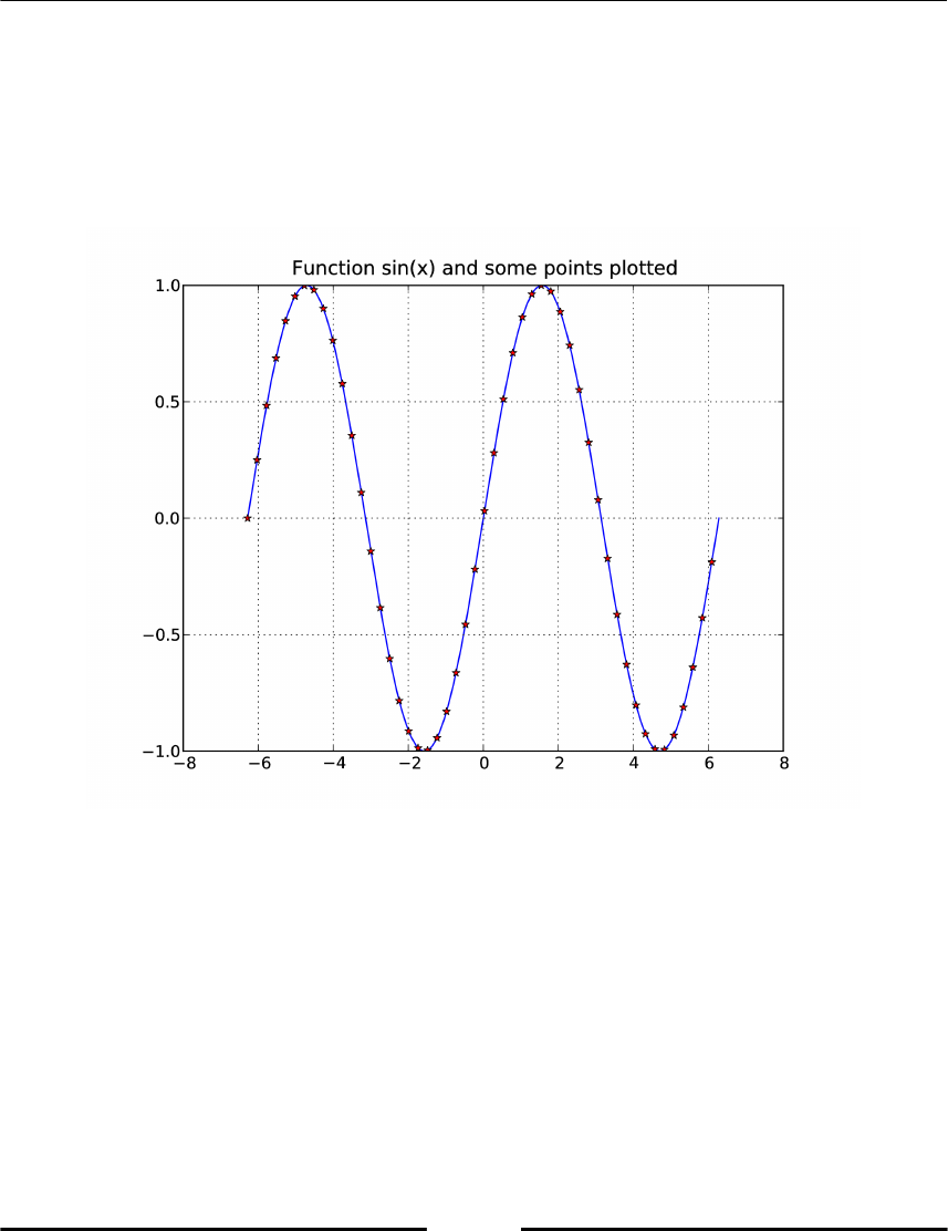
Plotting
[ 120 ]
plot(samples,sin(samples),'r*')
# add title and grid lines
title('Function sin(x) and some points plotted')
grid()
The result is shown in the following figure (Figure 6.1):
Figure 6.1: A plot of the function sin(x) with grid lines shown.

Plotting
[ 121 ]
As you can see, the standard plot is a solid blue curve. Each axis gets automatically scaled
to fit the values but can also be set manually. Color and plot options can be given after the
first two input arguments. Here, r* indicates red star-shaped markers. Formatting is
covered in more detail in the next section. The title command puts a title text string above
the plot area.
Calling plot multiple times will overlay the plots in the same window. To get a new clean
figure window, use figure(). The figure command might contain an integer, for
example, figure(2), which can be used to switch between figure windows. If there is no
figure window with that number, a new one is created, otherwise, the window is activated
for plotting and all subsequent plotting commands apply to that window.
Multiple plots can be explained using the legend function, along with adding labels to each
plot call. The following example fits polynomials to a set of points using the commands
polyfit and polyval, and plots the result with a legend:
# —Polyfit example—
x = range(5)
y = [1,2,1,3,5]
p2 = polyfit(x,y,2)
p4 = polyfit(x,y,4)
# plot the polynomials and points
xx = linspace(-1,5,200)
plot(xx, polyval(p2, xx), label='fitting polynomial of degree 2')
plot(xx, polyval(p4, xx),
label='interpolating polynomial of degree 4')
plot(x,y,'*')
# set the axis and legend
axis([-1,5,0,6])
legend(loc='upper left', fontsize='small')

Plotting
[ 122 ]
Here you can also see how to manually set the range of the axis using
axis([xmin,xmax,ymin,ymax]). The legend command takes optional arguments on
placement and formatting; in this case the legend is put in the upper-left corner and typeset
with a small font size, as shown in the following figure (Figure 6.2).
Figure 6.2: Two polynomials fitted to the same points.
As final examples for basic plotting, we demonstrate how to do scatter plots and
logarithmic plots in two dimensions.
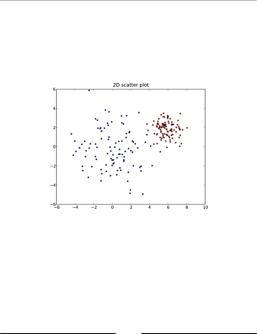
Plotting
[ 123 ]
Example of 2D point scatter plot:
# create random 2D points
import numpy
x1 = 2*numpy.random.standard_normal((2,100))
x2 = 0.8*numpy.random.standard_normal((2,100)) + array([[6],[2]])
plot(x1[0],x1[1],'*')
plot(x2[0],x2[1],'r*')
title('2D scatter plot')
Figure 6.3(a): An example of a scatter plot
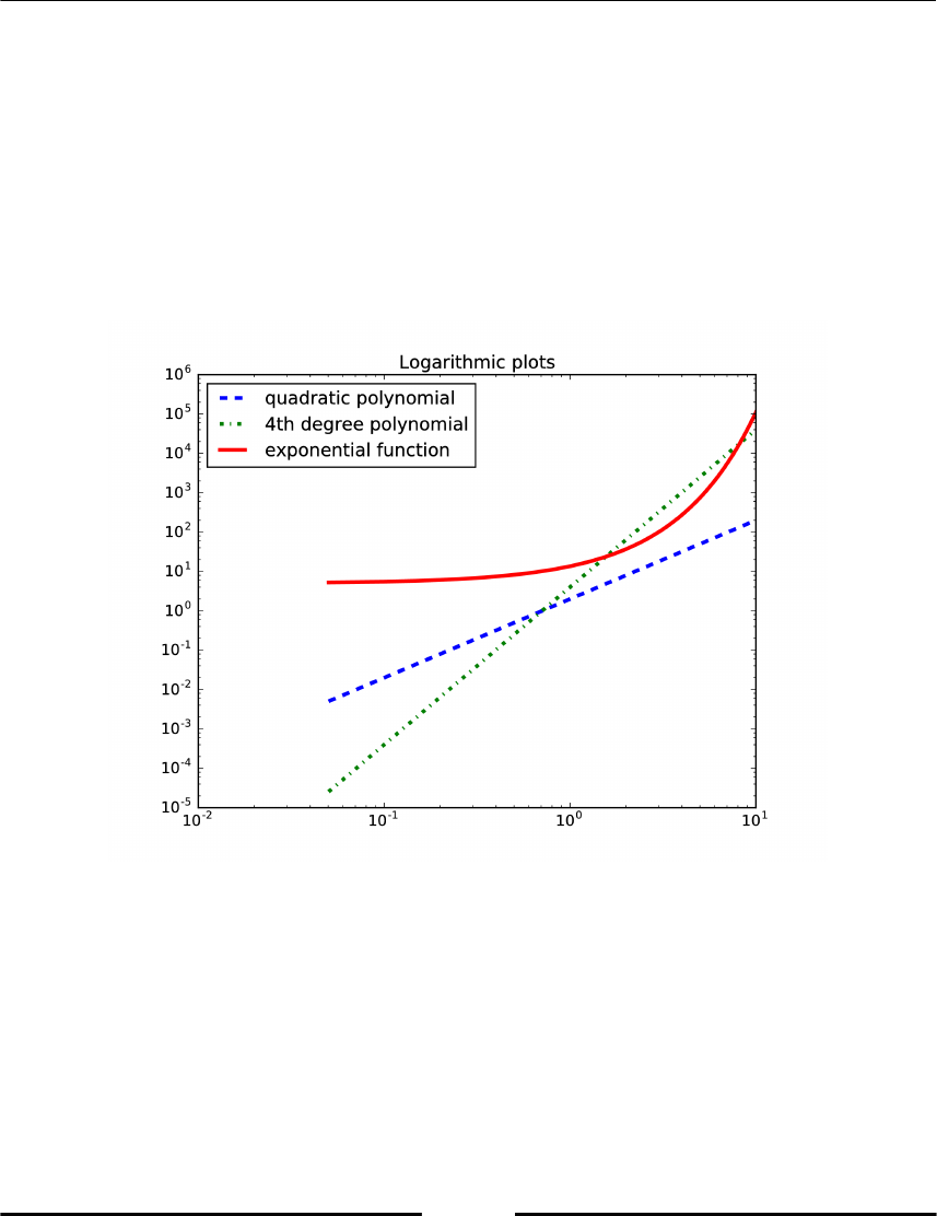
Plotting
[ 124 ]
The following code is an example of a logarithmic plot using loglog:
# log both x and y axis
x = linspace(0,10,200)
loglog(x,2*x**2, label = 'quadratic polynomial',
linestyle = '-', linewidth = 3)
loglog(x,4*x**4, label = '4th degree polynomial',
linestyle = '-.', linewidth = 3)
loglog(x,5*exp(x), label = 'exponential function', linewidth = 3)
title('Logarithmic plots')
legend(loc = 'best')
Figure 6.3(b): An example of a plot with logarithmic x and y axis
The examples shown in the preceding figure (Figure 6.3(a) and Figure 6.3(b)) used some
parameters of plot and loglog which allow special formatting. In the next section, we will
explain the parameters in more detail.
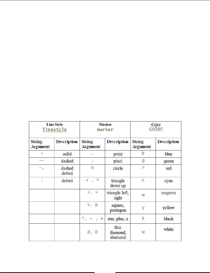
Plotting
[ 125 ]
Formatting
The appearance of figures and plots can be styled and customized to look how you want
them to look. Some important variables are linewidth, which controls the thickness of plot
lines; xlabel, ylabel, which set the axis labels, color for plot colors, and transparent
for transparency. This section will tell you how to use some of them. The following is an
example with more keywords:
k = 0.2
x = [sin(2*n*k) for n in range(20)]
plot(x, color='green', linestyle='dashed', marker='o',
markerfacecolor='blue', markersize=12, linewidth=6)
There are short commands that can be used if you only need basic style changes, for
example, setting the color and line style. The following table (Table 6.1) shows some
examples of these formatting commands. You may use either the short string syntax
plot(...,'ro-'), or the more explicit syntax plot(..., marker='o', color='r',
linestyle='-').
Table 6.1: Some common plot formatting arguments
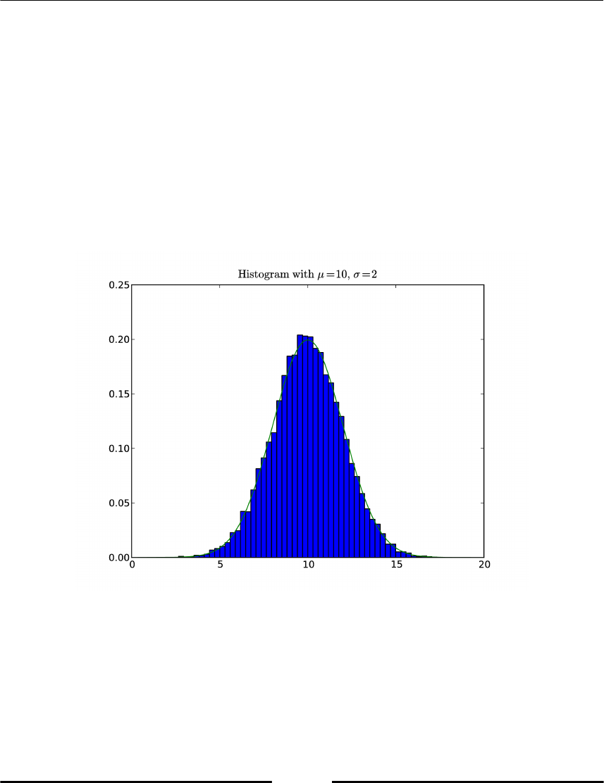
Plotting
[ 126 ]
To set the color to green with the 'o' marker we write:
plot(x,'go')
To plot histograms instead of regular plots, the hist command is used:
# random vector with normal distribution
sigma, mu = 2, 10
x = sigma*numpy.random.standard_normal(10000)+mu
hist(x,50,normed=1)
z = linspace(0,20,200)
plot(z, (1/sqrt(2*pi*sigma**2))*exp(-(z-mu)**2/(2*sigma**2)),'g')
# title with LaTeX formatting
title('Histogram with '.format(mu,sigma))
Figure 6.4 normal distribution with 50 bins and a green curve indicating the true
distribution
The resulting plot looks similar to the preceding figure (Figure 6.4). The title, and any other
text, can be formatted using LaTeX to show mathematical formulas. LaTeX formatting is
enclosed within a pair of $ signs. Also, note the string formatting done using the format
method, refer to section Strings in Chapter 2, Variables and Basic Types.
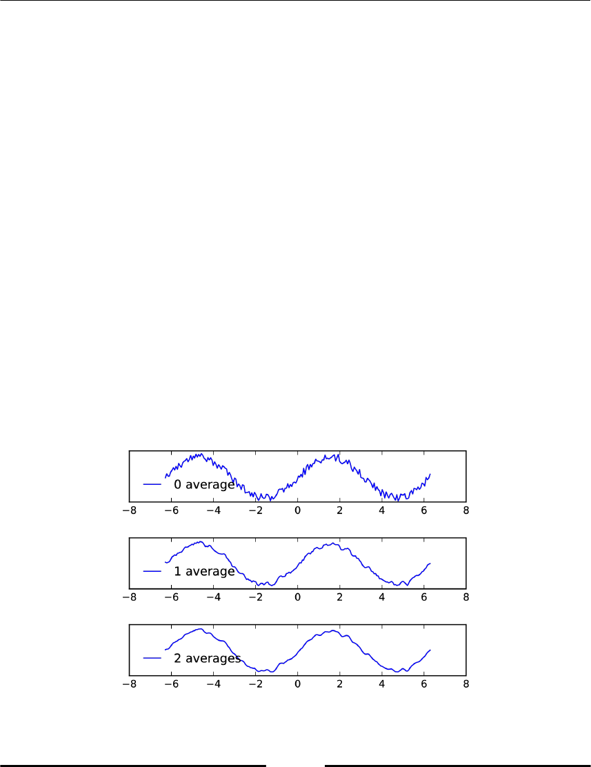
Plotting
[ 127 ]
Sometimes the brackets for the string formatting interfere with LaTeX bracket
environments. If this occurs, replace the LaTeX bracket with a double bracket, for example,
x_{1} should be replaced with x_{{1}}. The text might contain sequences that overlap
with string escape sequences, for example, \tau will be interpreted as the tab character \t.
An easy workaround is to add r before the string, for example r'\tau'; this makes it a
raw string.
Placing several plots in one figure window can be done using the subplot command.
Consider the following example, which iteratively averages out the noise on a sine curve.
def avg(x):
""" simple running average """
return (roll(x,1) + x + roll(x,-1)) / 3
# sine function with noise
x = linspace(-2*pi, 2*pi,200)
y = sin(x) + 0.4*rand(200)
# make successive subplots
for iteration in range(3):
subplot(3, 1, iteration + 1)
plot(x,y, label = '{:d} average{}'.format(iteration, 's' if iteration >
1 else ''))
yticks([])
legend(loc = 'lower left', frameon = False)
y = avg(y) #apply running average
subplots_adjust(hspace = 0.7)
Figure 6.5: An example of plotting several times in the same figure window.
Plotting
[ 128 ]
The function avg uses a roll call to shift all values of the array. subplot takes three
arguments: the number of vertical plots, the number of horizontal plots, and an index
indicating which location to plot in (counted row-wise). Note that we used the
subplots_adjust command to add extra space to adjust the distance between both the
subplots.
A useful command is savefig which lets you save a figure as an image (this can also be
done from the figure window). Many image and file formats are supported by this
command, they are specified by the filename's extension as:
savefig('test.pdf') # save to pdf
or
savefig('test.svg') # save to svg (editable format)
You can place the image against a non-white background, for example, a webpage. For this,
the transparent parameter can be set to make the figure's background transparent:
savefig('test.pdf', transparent=True)
If you intend to embed a figure into a LaTeX document, it is recommended that you reduce
the surrounding white space by setting the figure's bounding box tight around the drawing,
as shown here:
savefig('test.pdf', bbox_inches='tight')
Meshgrid and contours
A common task is a graphical representation of a scalar function over a rectangle:
For this, first we have to generate a grid on the rectangle [a,b] x [c,d]. This is done using the
meshgrid command:
n = ... # number of discretization points along the x-axis
m = ... # number of discretization points along the x-axis
X,Y = meshgrid(linspace(a,b,n), linspace(c,d,m))
Plotting
[ 129 ]
X and Y are arrays with (n,m) shape such that contains the coordinates of the grid point as
shown in the next figure (Figure 6.6):
Figure 6.6: A rectangle discretized by meshgrid
A rectangle discretized by meshgrid will be used to visualize the behavior of an iteration.
Bur first we will use it to plot level curves of a function. This is done by the command
contour.
As an example we choose Rosenbrock's banana function:
It is used to challenge optimization methods. The function values descend towards a
banana-shaped valley, which itself decreases slowly towards the function’s global minimum
at (1, 1).
First we display the level curves using contour.
rosenbrockfunction = lambda x,y: (1-x)**2+100*(y-x**2)**2
X,Y = meshgrid(linspace(-.5,2.,100), linspace(-1.5,4.,100))
Z = rosenbrockfunction(X,Y)
contour(X,Y,Z,logspace(-0.5,3.5,20,base=10),cmap='gray')
title('Rosenbrock Function: ')
xlabel('x')
ylabel('y')
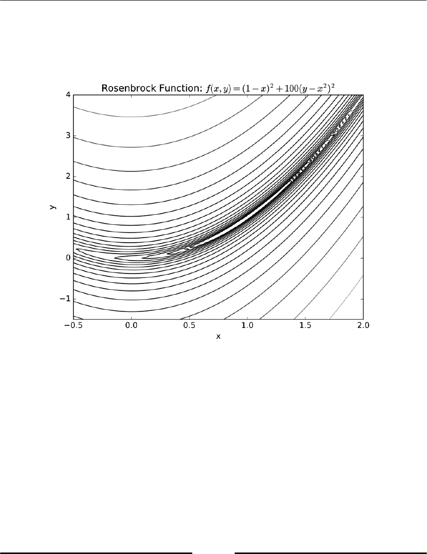
Plotting
[ 130 ]
This plots the level curve at the levels given by the fourth parameter and uses the colormap
gray. Furthermore, we used logarithmically spaced steps from 100.5 to 103 using the function
logscale to define the levels, as shown in the next figure.
Figure 6.7: A contour plot of Rosenbrock function
In the preceding example, an anonymous function indicated by the keyword lambda is
used to keep the code compact. Anonymous functions are explained in section Anonymous
functions – the lambda keyword in Chapter 7, Functions, Anonymous functions. If levels are not
given as arguments to contour, the function chooses appropriate levels by itself .
The contourf function performs the same function as contour but fills the plot with colors
according to different levels. Contour plots are ideal for visualizing the behavior of a
numerical method. We illustrate this here by showing the iterations of an optimization
method.
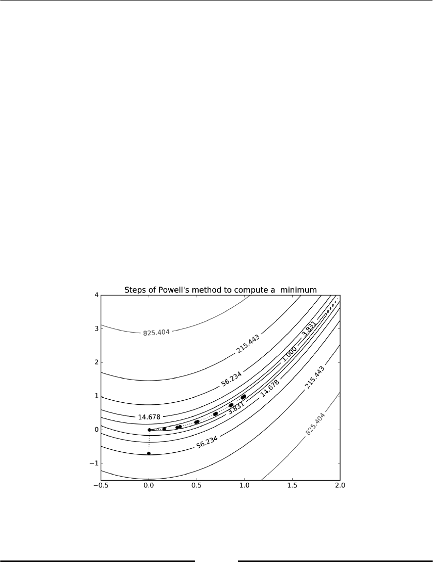
Plotting
[ 131 ]
We continue the preceding example and depict the steps towards the minimum of the
Rosenbrock function generated by Powell's method, [27], which we will apply to find the
minimum of the Rosenbrock function:
import scipy.optimize as so
rosenbrockfunction = lambda x,y: (1-x)**2+100*(y-x**2)**2
X,Y=meshgrid(linspace(-.5,2.,100),linspace(-1.5,4.,100))
Z=rosenbrockfunction(X,Y)
cs=contour(X,Y,Z,logspace(0,3.5,7,base=10),cmap='gray')
rosen=lambda x: rosenbrockfunction(x[0],x[1])
solution, iterates = so.fmin_powell(rosen,x0=array([0,-0.7]),retall=True)
x,y=zip(*iterates)
plot(x,y,'ko') # plot black bullets
plot(x,y,'k:',linewidth=1) # plot black dotted lines
title("Steps of Powell's method to compute a minimum")
clabel(cs)
The iterative method fmin_powell applies Powell's method to find a minimum. It is
started by a given start value of x0 and reports all iterates when the option retall=True is
given. After sixteen iterations, the solution x=0, y=0 was found. The iterations are depicted
as bullets in the following contour plot (Figure 6.8).
Figure 6.8: A contour plot of Rosenbrock function with a search path of an optimization
method
Plotting
[ 132 ]
contour also creates a contour set object that we assigned to the variable cs. This is then
used by clabel to annotate the levels of the corresponding function values, as shown in the
preceding figure (Figure 6.8).
Images and contours
Let us take a look at some examples of visualizing arrays as images. The following function
will create a matrix of color values for the Mandelbrot fractal. Here we consider a fixed
point iteration, that depends on a complex parameter c:
Depending on the choice of this parameter it may or may not create a bounded sequence of
complex values zn.
For every value of c, we check if zn exceeds a prescribed bound. If it remains below the
bound within maxit iterations, we assume the sequence to be bounded.
Note how, in the following piece of code,meshgrid is used to generate a matrix of complex
parameter values c:
def mandelbrot(h,w, maxit=20):
X,Y = meshgrid(linspace(-2, 0.8, w), linspace(-1.4, 1.4, h))
c = X + Y*1j
z = c
exceeds = zeros(z.shape, dtype=bool)
for iteration in range(maxit):
z = z**2 + c
exceeded = abs(z) > 4
exceeds_now = exceeded & (logical_not(exceeds))
exceeds[exceeds_now] = True
z[exceeded] = 2 # limit the values to avoid overflow
return exceeds
imshow(mandelbrot(400,400),cmap='gray')
axis('off')
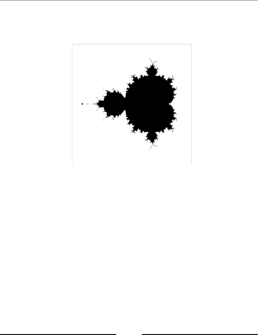
Plotting
[ 133 ]
The command imshow displays the matrix as an image. The selected color map shows the
regions where the sequence appeared unbounded in white and others in black. Here we
used axis('off') to turn off the axis as this might be not so useful for images.
Figure 6.9: An example of using imshow to visualize a matrix as an image.
By default, imshow uses interpolation to make the images look nicer. This is clearly seen
when the matrices are small. The next figure shows the difference between using:
imshow(mandelbrot(40,40),cmap='gray')
and
imshow(mandelbrot(40,40), interpolation='nearest', cmap='gray')
Plotting
[ 134 ]
In the second example, pixel values are just replicated.
Figure 6.10: The difference between using the linear interpolation of imshow
compared to using nearest neighbor interpolation
For more details on working and plotting with images using Python refer to [30].
Matplotlib objects
Till now, we have used the pyplot module of matplotlib. This module makes it easy for us
to use the most important plot commands directly. Mostly, we are interested in creating a
figure and display it immediately. Sometimes, though, we want to generate a figure that
should be modified later by changing some of its attributes. This requires us to work with
graphical objects in an object-oriented way. In this section, we will present some basic steps
to modify figures. For a more sophisticated object oriented approach to plotting in Python,
you have to leave pyplot and have to dive directly into matplotlib with its extensive
documentation.

Plotting
[ 135 ]
The axes object
When creating a plot that should be modified later, we need references to a figure and an
axes object. For this we have to create a figure first and then define some axes and their
location in the figure. And we should not forget to assign these objects to a variable:
fig = figure()
ax = subplot(111)
A figure can have several axes objects depending on the use of subplot. In a second step
plots are associated with a given axes object:
fig = figure(1)
ax = subplot(111)
x = linspace(0,2*pi,100)
# We set up a function that modulates the amplitude of the sin function
amod_sin = lambda x: (1.-0.1*sin(25*x))*sin(x)
# and plot both...
ax.plot(x,sin(x),label = 'sin')
ax.plot(x, amod_sin(x), label = 'modsin')
Here we used an anonymous function indicated by the lambda keyword . We will explain
this construct later in section Anonymous functions – the lambda keyword in Chapter 7,
Functions. In fact, these two plot commands fill the list ax.lines with two Lines2D objects:
ax.lines #[<matplotlib.lines.Line2D at ...>, <matplotlib.lines.Line2D at
...>]
It is a good practice to use labels so that we can later identify objects in an easy way:
for il,line in enumerate(ax.lines):
if line.get_label() == 'sin':
break
We set up now things in a way that allows further modifications. The figure we got so far is
shown in preceding figure (Figure 6.11, left).

Plotting
[ 136 ]
Modifying line properties
We just identified a particular line object by its label. It is an element of the list ax.lines
list with the index il . All its properties are collected in a dictionary
dict_keys(['marker', 'markeredgewidth', 'data', 'clip_box',
'solid_capstyle', 'clip_on', 'rasterized', 'dash_capstyle', 'path',
'ydata', 'markeredgecolor', 'xdata', 'label', 'alpha', 'linestyle',
'antialiased', 'snap', 'transform', 'url',
'transformed_clip_path_and_affine', 'clip_path', 'path_effects',
'animated', 'contains', 'fillstyle', 'sketch_params', 'xydata',
'drawstyle', 'markersize', 'linewidth', 'figure', 'markerfacecolor',
'pickradius', 'agg_filter', 'dash_joinstyle', 'color', 'solid_joinstyle',
'picker', 'markevery', 'axes', 'children', 'gid', 'zorder', 'visible',
'markerfacecoloralt'])
which can be obtained by the command:
ax.lines[il].properties()
They can be changed by corresponding setter methods. Let us change the line style of the
sine – curve:
ax.lines[il].set_linestyle('-.')
ax.lines[il].set_linewidth(2)
We can even modify the data, as shown:
ydata=ax.lines[il].get_ydata()
ydata[-1]=-0.5
ax.lines[il].set_ydata(ydata)
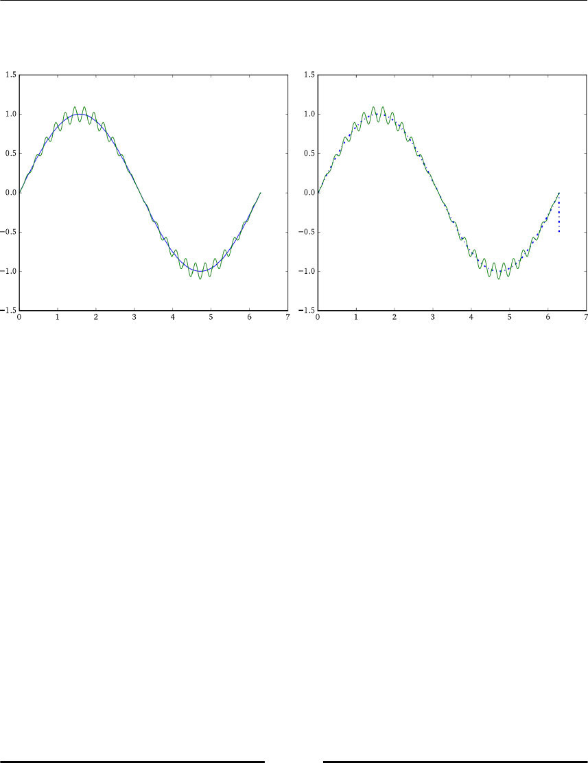
Plotting
[ 137 ]
The result is shown in the next figure(Figure 6.11, right):
Figure 6.11: The amplitude modulated sine-function (left) and a curve with the
last data point corrupted (right).
Annotations
One useful axes method is annotate. It sets an annotation at a given position and points,
with an arrow, to another position in the drawing. The arrow can be given properties in a
dictionary:
annot1=ax.annotate('amplitude modulated\n curve', (2.1,1.0),(3.2,0.5),
arrowprops={'width':2,'color':'k',
'connectionstyle':'arc3,rad=+0.5',
'shrink':0.05},
verticalalignment='bottom', horizontalalignment='left',fontsize=15,
bbox={'facecolor':'gray', 'alpha':0.1, 'pad':10})
annot2=ax.annotate('corrupted data', (6.3,-0.5),(6.1,-1.1),
arrowprops={'width':0.5,'color':'k','shrink':0.1},
horizontalalignment='center', fontsize=12)
In the first annotation example above, the arrow points to a point with the coordinates (2.1,
1.0) and the left bottom coordinate of the text is (3.2, 0.5). If not otherwise specified, the
coordinates are given in the convenient data-coordinate system, which refers to the data
used to generate the plots.

Plotting
[ 138 ]
Furthermore, we demonstrated a couple of arrow properties specified by the arrowprop
dictionary. You can scale the arrow by the shrink key. The setting 'shrink':0.05
reduces the arrow size by 5% to keep a distance to the curve it points to. You can let the
arrow follow a spline arc or give it other shapes using the connectionstyle key.
Text properties or even a bounding box around the text can be made by extra keyword
arguments to the annotate method, refer to the following figure (Figure 6.12, left):
Experimenting with annotations requires sometimes to remove attempts that we would like
to reject. Therefore we assigned the annotate object to a variable, which allows us to remove
the annotation by its remove method:
annot1.remove()
Filling areas between curves
Filling is an ideal tool to highlight differences between curves, such as noise on top of
expected data, approximations versus exact functions, and so on.
Filling is done by the axis method
ax.fill_between(x,y1,y2)
For the next figure we used:
axf = ax.fill_between(x, sin(x), amod_sin(x), facecolor='gray')
where is a very convenient parameter that needs a Boolean array to specify the additional
filling conditions.
axf = ax.fill_between(x, sin(x), amod_sin(x),where=amod_sin(x)-sin(x) > 0,
facecolor=’gray’)
The Boolean array which selects the regions to fill is amod_sin(x)-sin(x) > 0.
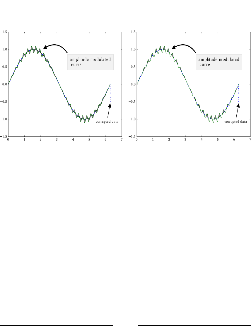
Plotting
[ 139 ]
The next figure shows the curve with both variants of filling areas:
Figure 6.12: The amplitude modulated sin-function with annotations and filled
areas(left) and a modified figure with only partially filled areas by using the
where parameter (right).
If you test these commands yourself, do not forget to remove the complete filling before you
try out the partial filling, otherwise you will not see any change:
axf.remove()
Related filling commands are fill and fill_betweenx.
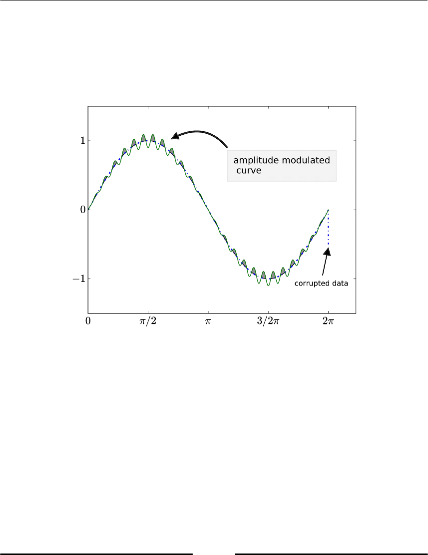
Plotting
[ 140 ]
Ticks and ticklabels
Figures in talks, posters, and publications look much nicer if they are not overloaded with
unnecessary information. You want to direct the spectator to those parts that contain the
message. In our example, we clean up the picture by removing ticks from the x-axis and y-
axis and by introducing problem related tick labels:
Figure 6.13: The completed example of the amplitude modulated sine – function with
annotations and filled areas and modified ticks and tick labels.
ax.set_xticks(array([0,pi/2,pi,3/2*pi,2*pi]))
ax.set_xticklabels(('$0$','$\pi/2$','$\pi$','$3/2 \pi$','$2
\pi$'),fontsize=18)
ax.set_yticks(array([-1.,0.,1]))
ax.set_yticklabels(('$-1$','$0$','$1$'),fontsize=18)

Plotting
[ 141 ]
Note that we used LaTeX formatting in the strings to represent Greek letters, to set formulas
correctly, and to use a LaTeX font. It is also a good practice to increase the font size so that
the resulting figure can be scaled down into a text document without affecting the
readability of the axes. The final result of this guiding example is shown in the previous
figure (Figure 6.13).
Making 3D plots
There are some useful matplotlib tool kits and modules that can be used for a variety of
special purposes. In this section, we describe a method for producing 3D-plots.
The mplot3d toolkit provides 3D plotting of points, lines, contours, surfaces, and all other
basic components as well as 3D rotation and scaling. Making a 3D plot is done by adding
the keyword projection='3d' to the axes object as shown in the following example:
from mpl_toolkits.mplot3d import axes3d
fig = figure()
ax = fig.gca(projection='3d')
# plot points in 3D
class1 = 0.6 * random.standard_normal((200,3))
ax.plot(class1[:,0],class1[:,1],class1[:,2],'o')
class2 = 1.2 * random.standard_normal((200,3)) + array([5,4,0])
ax.plot(class2[:,0],class2[:,1],class2[:,2],'o')
class3 = 0.3 * random.standard_normal((200,3)) + array([0,3,2])
ax.plot(class3[:,0],class3[:,1],class3[:,2],'o')
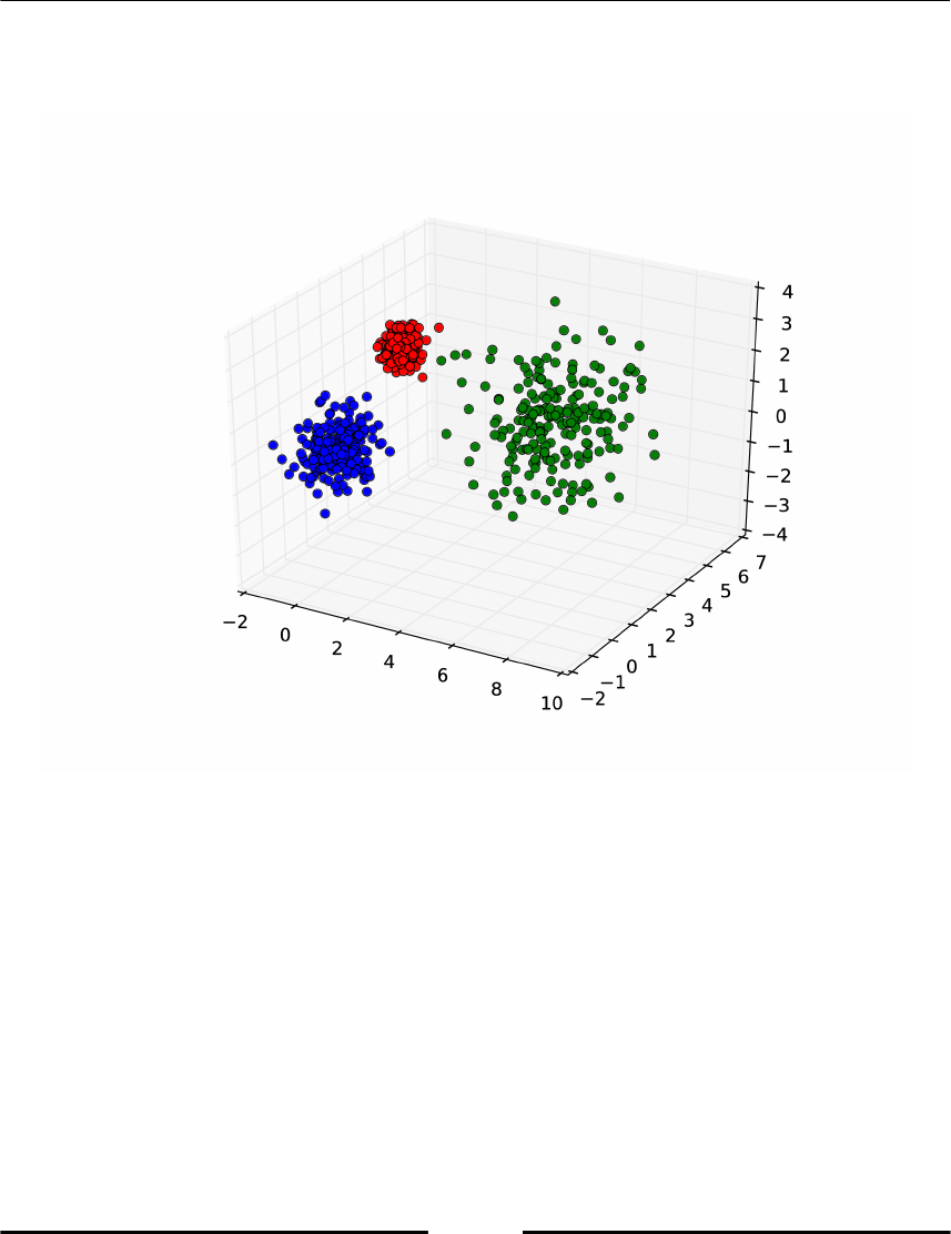
Plotting
[ 142 ]
As you can see, you need to import the axes3D type from mplot3d. The resulting plot
displays the scattered 3D-data which can be seen in the following figure (Figure 6.14)
Figure 6.14: Plotting 3D data using mplot3d toolkit
Plotting surfaces is just as easy. The following example uses the built-in function
get_test_data to create a sample data for plotting a surface. Consider the following
example of a surface plot with transparency.
X,Y,Z = axes3d.get_test_data(0.05)
fig = figure()
ax = fig.gca(projection='3d')
# surface plot with transparency 0.5
ax.plot_surface(X,Y,Z,alpha=0.5)
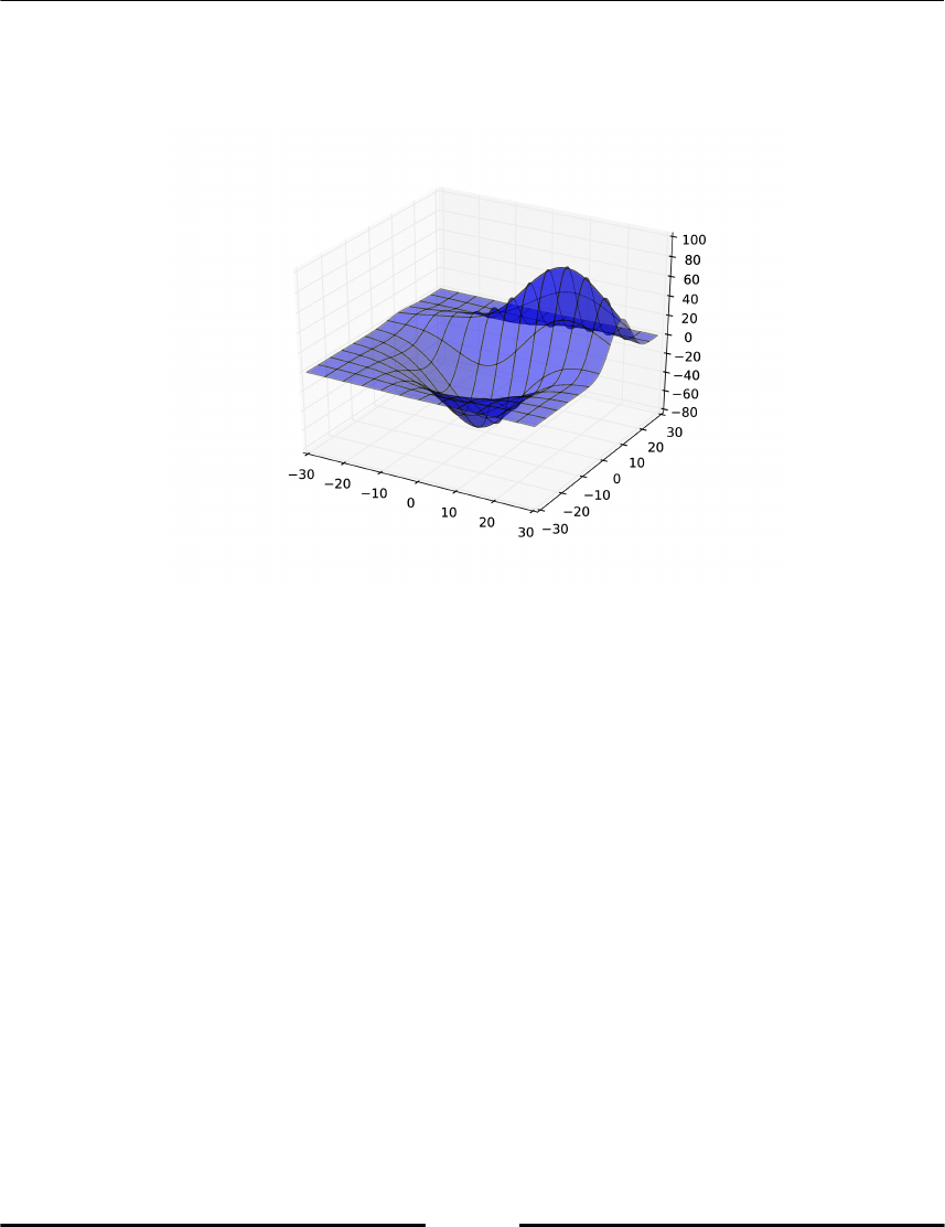
Plotting
[ 143 ]
The alpha value sets the transparency. The surface plot is shown in the following figure
(Figure 6.15).
Figure 6.15: Example for plotting a surface mesh with three 2D projections.
You can also plot contours in any of the coordinate projections as in the next example.
fig = figure()
ax = fig.gca(projection = '3d')
ax.plot_wireframe(X,Y,Z,rstride = 5,cstride = 5)
# plot contour projection on each axis plane
ax.contour(X,Y,Z, zdir='z',offset = -100)
ax.contour(X,Y,Z, zdir='x',offset = -40)
ax.contour(X,Y,Z, zdir='y',offset = 40)
# set axis limits
ax.set_xlim3d(-40,40)
ax.set_ylim3d(-40,40)
ax.set_zlim3d(-100,100)
# set labels
ax.set_xlabel('X axis')
ax.set_ylabel('Y axis')
ax.set_zlabel('Z axis')
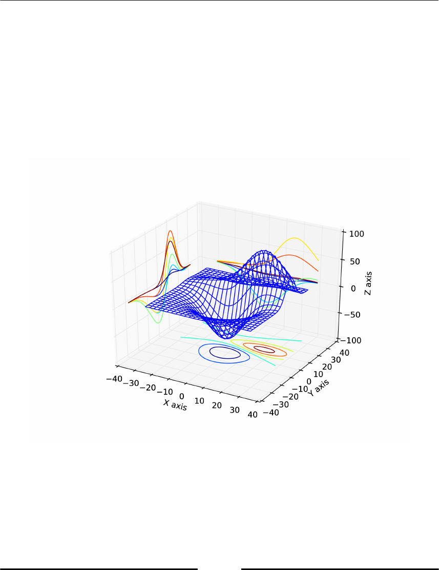
Plotting
[ 144 ]
Note the commands for setting the axis limits. The standard matplotlib commands for
setting the axis limits are axis([-40, 40, -40, 40]), this works fine for 2D plots.
However, axis([-40,40,-40,40,-40,40]) does not work. For 3D plots you need to use
the object oriented version of the commands, ax.set_xlim3d(-40,40) and likewise. The
same goes for labeling the axis; note the commands for setting the labels. For 2D plots you
can do xlabel(’X axis’) and ylabel(’Y axis’) but there is no zlabel command.
Instead, in 3D plots you need to use ax.set_xlabel(’X axis’) and likewise, as shown in
the preceding example.
The resulting figure from this code is the following
There are many options for formatting the appearance of the plots, including color and
transparency of surfaces. The mplot3d documentation website, [23], has the details.

Plotting
[ 145 ]
Making movies from plots
If you have data that evolves, you might want to save it as a movie besides showing it in a
figure window, similar to the savefig command. One way to do this is with the visvis
module available at visvis (refer to [37] for more information).
Here is a simple example of evolving a circle using an implicit representation. Let the circle
be represented by the zero level, , of a function . Alternatively, consider
the disk inside the zero set. If the value of f decreases at a rate v then the circle
will move outward with rate .
This can be implemented as:
import visvis.vvmovie as vv
# create initial function values
x = linspace(-255,255,511)
X,Y = meshgrid(x,x)
f = sqrt(X*X+Y*Y) - 40 #radius 40
# evolve and store in a list
imlist = []
for iteration in range(200):
imlist.append((f>0)*255)
f -= 1 # move outwards one pixel
vv.images2swf.writeSwf('circle_evolution.swf',imlist)
The result is a Flash movie (*.swf file) of a growing black circle, as shown in the next figure
(Figure 6.16):
Figure 6.16: An example of evolving a circle

Plotting
[ 146 ]
In this example, a list of arrays was used to create the movie. The visvis module can also
save an GIF animation and on certain platforms an AVI animation (*.gif and *.avi files), and
there is also the possibility to capturing movie frames directly from the figure window.
These options, however, require some more packages to be installed on your system (for
example, PyOpenGL and PIL, the Python Imaging Library). See the documentation on the
visvis webpage for more details.
Another option is to use savefig to create images, one for each frame.
# create initial function values
x = linspace(-255,255,511)
X,Y = meshgrid(x,x)
f = sqrt(X*X+Y*Y) - 40 #radius 40
for iteration in range(200):
imshow((f>0)*255)
gray()
axis('off')
savefig('circle_evolution_{:d}.png'.format(iteration))
f -= 1
These images can then be combined using a standard video editing software, for example,
Mencoder or ImageMagick. This approach has the advantage that you can make high-
resolution videos by saving high-resolution images.
Summary
A graphical representation is the most compact form in which to present mathematical
results or the behavior of an algorithm. This chapter provided you with the basic tools for
plotting and introduced you to a more sophisticated way to work with graphical objects,
such as figures, axes, and lines in an object-oriented way.
In this chapter, you learned how to make plots, not only classical x/y-plots but also 3D-plots
and histograms. We gave you an appetizer on making films. You also saw how to modify
plots considering them to be graphical objects with related methods and attributes which
can be set, deleted, or modified.
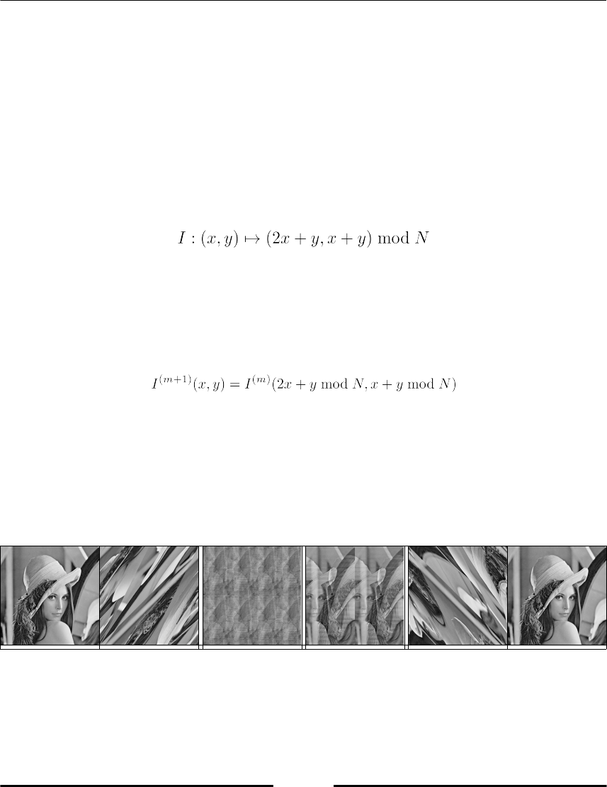
Plotting
[ 147 ]
Exercises
Ex. 1 → Write a function that plots an ellipse given its center coordinates (x,y), the half axis a
and b rotation angle θ.
Ex. 2 → Write a short program that takes a 2D array, e.g., the preceding Mandelbrot contour
image, and iteratively replace each value by the average of its neighbors. Update a contour
plot of the array in a figure window to animate the evolution of the contours. Explain the
behavior.
Ex. 3 → Consider an N × N matrix or image with integer values. The mapping
is an example of a mapping of a toroidal square grid of points onto itself. This has the
interesting property that it distorts the image by shearing and then moving the pieces
outside the image back using the modulu function mod. Applied iteratively, this results in
randomizing the image in a way that eventually returns the original. Implement the
following sequence:
and save out the first N steps to files or plot them in a figure window.
As an example image, you can use the classic 512 × 512 Lena test image from scipy.misc.
from scipy.misc import lena
I = lena()
The result should look like this:
………
01 128 256 511 512

Plotting
[ 148 ]
Compute the x and y mappings and use array indexing (refer to section
Array Indexing in Chapter 5, Advance Array Concepts) to copy the pixel
values.
Ex. 4 → Reading and plotting on images. SciPy comes with the imread function (in the
scipy.misc module) for reading images, (refer to section Reading and Writing Images in
Chapter 12, Input and output). Write a short program that reads an image from file and plots
the image contour at a given gray level value overlaid on the original image.
You can get a gray level version of the image by averaging the color
channels like this: mean(im,axis=2)
Ex. 5 → Image edges. The zero crossings of the 2D Laplacian are a good indication of image
edges. Modify the program in the previous exercise to use the gaussian_laplace or
laplace function from the scipy.ndimage module to compute the 2D Laplacian and
overlay the edges on top of the image.
Ex. 6 → Reformulate the Mandelbrod fractal example (see section Images and Contours) by
using orgid instead of meshgrid, see also the explanation ogrid in Function of two variables
in Chapter 5, Advanced Array Concepts. What is the difference between orgid, mgrid, and
meshgrid?
7
Functions
This chapter introduces functions, a fundamental building block in programming. We show
how to define them, how to handle input and output, how to properly use them, and how
to treat them as objects.
Basics
In mathematics, a function is written as a map that uniquely assigns an element y from the
range R to every element x from the domain D.
This is expressed by f : D → R
Alternatively, when considering particular elements x and y, one writes f : x → y
Here, f is called the name of the function and f(x) is its value when applied to x. Here, x is
sometimes called the argument of f. Let's first look at an example before considering
functions in Python.
For example, D = ℝ x ℝ and y = f(x1, x2) = x1– x2. This function maps two real numbers to
their difference.
In mathematics, functions can have numbers, vectors, matrices, and even other functions as
arguments. Here is an example of a function with mixed arguments:
.

Functions
[ 150 ]
In this case, a number is returned. When working with functions, we have to distinguish
between two different steps:
The definition of the function
The evaluation of the function, that is, the computation of f(x) for a given value of
x
The first step is done once, while the second can be performed many times for various
arguments. Functions in programming languages follow the same concept and apply it to a
wide range of types of input arguments, for example, strings, lists, or any object. We
demonstrate a definition of the function by considering the given example again:
def subtract(x1, x2):
return x1 - x2
The keyword def indicates that we are going to define a function. subtract is the
function’s name and x1 and x2 are its parameters. The colon indicates that we are using a
block command and the value that is returned by the function follows the return keyword.
Now, we can evaluate this function. This function is called with its parameters replaced by
input arguments:
r = subtract(5.0, 4.3)
The result 0.7 is computed and assigned to the r variable.
Parameters and arguments
When defining a function, its input variables are called the parameters of the function. The
input used when executing the function is called its argument.
Passing arguments – by position and by keyword
We will consider the previous example again, where the function takes two parameters,
namely x1 and x2.

Functions
[ 151 ]
Their names serve to distinguish the two numbers, which in this case cannot be
interchanged without altering the result. The first parameter defines the number from
which the second parameter is subtracted. When subtract is called, every parameter is
replaced by an argument. Only the order of the arguments matters; the arguments can be
any objects. For instance, we may call the following:
z = 3
e = subtract(5,z)
Besides this standard way of calling a function, which is by passing the arguments by
position, it might sometimes be convenient to pass arguments using keywords. The names
of the parameters are the keywords; consider the following instance:
z = 3
e = subtract(x2 = z, x1 = 5)
Here, the arguments are assigned to the parameters by name and not by position in the call.
Both ways of calling a function can be combined so that the arguments given by position
come first and the arguments given by keyword follow last. We show this by using
the function plot, which was described in Chapter 6, Plotting:
plot(xp, yp, linewidth = 2,label = 'y-values')
Changing arguments
The purpose of parameters is to provide the function with the necessary input data.
Changing the value of the parameter inside the function normally has no effect on its value
outside the function:
def subtract(x1, x2):
z = x1 - x2
x2 = 50.
return z
a = 20.
b = subtract(10, a) # returns -10
a # still has the value 20
This applies to all immutable arguments, such as strings, numbers, and tuples. The situation
is different if mutable arguments, such as lists or dictionaries, are changed.

Functions
[ 152 ]
For example, passing mutable input arguments to a function and changing them inside the
function can change them outside the function too:
def subtract(x):
z = x[0] - x[1]
x[1] = 50.
return z
a = [10,20]
b = subtract(a) # returns -10
a # is now [10, 50.0]
Such a function misuses its arguments to return results. We strongly dissuade you from
such constructions and recommend that you do not change input arguments inside the
function (for more information refer to Default Arguments section).
Access to variables defined outside the local
namespace
Python allows functions to access variables defined in any of its enclosing program units.
These are called global variables, in contrast to local variables. The latter are only accessible
within the function. For example, consider the following code:
import numpy as np # here the variable np is defined
def sqrt(x):
return np.sqrt(x) # we use np inside the function
This feature should not be abused. The following code is an example of what not to do:
a = 3
def multiply(x):
return a * x # bad style: access to the variable a defined outside
When changing the variable a the function, multiply tacitly changes its behavior:
a=3
multiply(4) # returns 12
a=4
multiply(4) # returns 16

Functions
[ 153 ]
It is much better in that case to provide the variable as a parameter through the argument
list:
def multiply(x, a):
return a * x
Global variables can be useful when working with closures. Namespaces and scopes are
discussed more extensively in Chapter 11, Namespaces, Scopes, and Modules.
Default arguments
Some functions can have many parameters, and among them some might only be of interest
in nonstandard situations. It would be practical if arguments could automatically be set to
standard (default) values. We demonstrate the use of default arguments by looking at the
command norm in the scipy.linalg module. It computes various norms of matrices and
vectors.
The following snippet calls for computing the Frobenius norm of the 3 × 3 identity matrix
are equivalent (more on matrix norms can be found in [10]):
import scipy.linalg as sl
sl.norm(identity(3))
sl.norm(identity(3), ord = 'fro')
sl.norm(identity(3), 'fro')
Note that in the first call, no information about the ord keyword is given. How does Python
know that it should compute the Frobenius norm and not another norm, for example, the
Euclidean 2-norm?
The answer to the previous question is the use of default values. A default value is a value
already given by the function definition. If the function is called without providing this
argument, Python uses the value that the programmer provided when the function was
defined.
Suppose we call the function subtract only one argument; we get an error message:
TypeError: subtract() takes exactly 2 arguments (1 given)
To allow the omission of the argument x2, the definition of the function has to provide a
default value, for example:
def subtract(x1, x2 = 0):
return x1 - x2

Functions
[ 154 ]
To summarize, arguments can be given as positional arguments and keyword arguments.
All positional arguments have to be given first. You do not need to provide all keyword
arguments as long as those omitted arguments have default values in the function
definition.
Beware of mutable default arguments
The default arguments are set upon function definition. Changing mutable arguments
inside a function has a side effect when working with default values, for example:
def my_list(x1, x2 = []):
x2.append(x1)
return x2
my_list(1) # returns [1]
my_list(2) # returns [1,2]
Variable number of arguments
Lists and dictionaries may be used to define or call functions with a variable number of
arguments. Let's define a list and a dictionary as follows:
data = [[1,2],[3,4]]
style = dict({'linewidth':3,'marker':'o','color':'green'})
Then we can call the plot function using starred (*) arguments:
plot(*data,**style)
A variable name prefixed by * , such as *data in the preceding example, means that a list
that gets unpacked in the function call is provided. In this way, a list generates positional
arguments. Similarly, a variable name prefixed by **, such as **style in the example,
unpacks a dictionary to keyword arguments. Refer to the following figure (Figure 7.1):

Functions
[ 155 ]
Figure 7.1: Starred arguments in function calls
You might also want to use the reverse process, where all given positional arguments are
packed into a list and all keyword arguments are packed into a dictionary when passed to a
function.
In the function definition, this is indicated by parameters prefixed by * and **,
respectively. You will often find the *args and **kwargs parameters in code
documentation, refer Figure 7.2.
Figure 7.2: Starred arguments in function definitions
Functions
[ 156 ]
Return values
A function in Python always returns a single object. If a function has to return more than
one object, these are packed and returned as a single tuple object.
For instance, the following function takes a complex number z and returns its polar
coordinate representation as magnitude r and angle according to Euler’s formula:
And the Python counterpart would be this:
def complex_to_polar(z):
r = sqrt(z.real ** 2 + z.imag ** 2)
phi = arctan2(z.imag, z.real)
return (r,phi) # here the return object is formed
Here, we used the sqrt(x) NumPy function for the square root of a number x and
arctan2(x,y) for the expression tan-1(x/y).
Let us try our function:
z = 3 + 5j # here we define a complex number
a = complex_to_polar(z)
r = a[0]
phi = a[1]
The last three statements can be written more elegantly in a single line:
r,phi = complex_to_polar(z)
We can test our function by calling polar_to_comp; refer to Exercise 1.
If a function has no return statement, it returns the value None. There are many cases
where a function does not need to return any value. This could be because the variables
passed to a function may be subject to modification. Consider, for instance, the following
function:
def append_to_list(L, x):
L.append(x)
Functions
[ 157 ]
The preceding function does not return anything because it modifies one of the objects that
is given as an argument. We mentioned in Parameters and Arguments section why this is
useful. There are many methods that behave in the same way. To mention the list methods
only, the append, extend, reverse, and sort methods do not return anything (that is,
they return None ). When an object is modified by a method in this way, the modification is
called in-place. It is difficult to know whether a method changes an object, except by
looking at the code or the documentation.
Another reason for a function, or a method, not to return anything is when it prints out a
message or writes to a file.
The execution stops at the first occurring return statement. Lines after that statement are
dead code, which will never be executed:
def function_with_dead_code(x):
return 2 * x
y = x ** 2 # these two lines ...
return y # ... are never executed!
Recursive functions
In mathematics, many functions are defined recursively. In this section, we will show how
this concept can be used even when programming a function. This makes the relation of the
program to its mathematical counterpart very clear, which may ease the readability of the
program.
Nevertheless, we recommend that you use this programming technique with care,
especially within scientific computing. In most applications, the more straightforward
iterative approach is more efficient. This will become immediately clear from the following
example.
Chebyshev polynomials are defined by a three-term recursion:

Functions
[ 158 ]
Such a recursion needs to be initialized, that is, T0(x) =1, T1(x) = x.
In Python, this three term recursion can be realized by the following function definition:
def chebyshev(n, x):
if n == 0:
return 1.
elif n == 1:
return x
else:
return 2. * x * chebyshev(n - 1, x)
- chebyshev(n - 2 ,x)
The function is then called like this:
chebyshev(5, 0.52) # returns 0.39616645119999994
This example also illustrates the risk of dramatically wasting computation time. The
number of function evaluations increases exponentially with the recursion level and most of
these evaluations are just duplicates of previous computations. While it might be tempting
to use recursive programs for demonstrating the strong relation between code and
mathematical definition, a production code will avoid this programming technique (refer to
Exercise 6). We also refer to a technique called memoization (refer to [22] for more details)
that combines recursive programming with a caching technique to save replicated function
evaluations.
A recursive function usually has a level parameter. In the previous example, it is n. It is
used to control the function's two main parts:
The base case, here, the first two if branches
The recursive body, in which the function itself is called once or several times
with smaller level parameters.
The number of levels passed by an execution of a recursive function is called the recursion
depth. This quantity should not be too large; otherwise the computation might no longer be
effective and in the ultimate case, the following error will be raised:
RuntimeError: maximum recursion depth exceeded
The maximal recursion depth depends on the memory of the computer you use. This error
also occurs when the initialization step is missing in the function definition. We encourage
the use of recursive programs for very small recursion depths (for more information, refer
to the section Infinite Iteration of Chapter 9, Iterating.

Functions
[ 159 ]
Function documentation
You should document your functions using a string at the beginning. This is
called docstring:
def newton(f, x0):
"""
Newton's method for computing a zero of a function
on input:
f (function) given function f(x)
x0 (float) initial guess
on return:
y (float) the approximated zero of f
"""
...
When calling help(newton), you get this docstring displayed together with the call of this
function:
Help on function newton in module __main__:
newton(f, x0)
Newton's method for computing a zero of a function
on input:
f (function) given function f(x)
x0 (float) initial guess
on return:
y (float) the approximated zero of f
The docstring is internally saved as an attribute, __doc__, of the given function. In the
example, it's newton.__doc__. The minimal information you should provide in a docstring
is the purpose of the function and the description of the input and output objects. There are
tools to automatically generate full code documentation by collecting all docstrings in your
program (for more information refer to [32]).
Functions
[ 160 ]
Functions are objects
Functions are objects, like everything else in Python. One may pass functions as arguments,
change their names, or delete them. For example:
def square(x):
"""
Return the square of x
"""
return x ** 2
square(4) # 16
sq = square # now sq is the same as square
sq(4) # 16
del square # square doesn't exist anymore
print(newton(sq, .2)) # passing as argument
Passing functions as arguments is very common when applying algorithms in scientific
computing. The functions fsolve in scipy.optimize for computing a zero of a given
function or quad in scipy.integrate for computing integrals are typical examples.
A function itself can have a different number of arguments with differing types. So, when
passing your function f to another function g as argument, make sure that f has exactly the
form described in the docstring of g.
The docstring of fsolve gives information about its func parameter:
func -- A Python function or method which takes at least one
(possibly vector) argument.
Partial application
Let's start with an example of a function with two variables.
The function can be viewed as a function in two variables. Often one
considers ω not as a free variable but as a fixed parameter of a family of functions fω:
This interpretation reduces a function in two variables to a function in one variable, t, given
a fixed parameter value ω. The process of defining a new function by fixing (freezing) one
or several parameters of a function is called partial application.

Functions
[ 161 ]
Partial applications are easily created using the Python module functools, which provides
a function called partial for precisely this purpose. We illustrate this by constructing a
function that returns a sine for a given frequency:
import functools
def sin_omega(t, freq):
return sin(2 * pi * freq * t)
def make_sine(frequency):
return functools.partial(sin_omega, freq = frequency)
Using Closures
Using the view that functions are objects, partial applications can be realized by writing a
function, which itself returns a new function, with a reduced number of input arguments.
For instance, the function could be defined as follows:
def make_sine(freq):
"Make a sine function with frequency freq"
def mysine(t):
return sin_omega(t, freq)
return mysine
In this example the inner function mysine has access to the variable freq; it is neither a
local variable of this function nor is it passed to it via the argument list. Python allows such
a construction (refer to Namespaces section in Chapter 11, Namespaces, Scopes, and Modules).
Anonymous functions – the lambda
keyword
The keyword lambda is used in Python to define anonymous functions, that is; functions
without a name and described by a single expression. You might just want to perform an
operation on a function that can be expressed by a simple expression without naming this
function and without defining this function by a lengthy def block.
The name lambda originates from a special branch of calculus and
mathematical logic, the -calculus.
Functions
[ 162 ]
For instance, to compute the following expression, we may use SciPy’s function quad,
which requires the function to be integrated as its first argument and the integration bounds
as the next two arguments:
Here, the function to integrate is just a simple one-liner and we use the lambda keyword to
define it:
import scipy.integrate as si
si.quad(lambda x: x ** 2 + 5, 0, 1)
The syntax is as follows:
lambda parameter_list: expression
The definition of the lambda function can only consist of a single expression and in
particular, cannot contain loops. lambda functions are, just like other functions, objects and
can be assigned to variables:
parabola = lambda x: x ** 2 + 5
parabola(3) # gives 14
The lambda construction is always replaceable
It is important to note that lambda construction is only syntactic sugar in Python. Any
lambda construction may be replaced by an explicit function definition:
parabola = lambda x: x**2+5
# the following code is equivalent
def parabola(x):
return x ** 2 + 5
The main reason to use a construction is for very simple functions, when a full function
definition would be too cumbersome.

Functions
[ 163 ]
lambda functions provide a third way to make closures as we demonstrate by continuing
with the previous example:
We use the sin_omega function to compute the integral of the sine function for various
frequencies:
import scipy.integrate as si
for iteration in range(3):
print(si.quad(lambda x: sin_omega(x, iteration*pi), 0, pi/2.) )
Functions as decorators
In the partial application section, we saw how a function can be used to modify another
function. A decorator is a syntax element in Python that conveniently allows us to alter the
behavior of a function without changing the definition of the function itself. Let us start
with the following situation:
Assume that we have a function that determines the degree of sparsity of a matrix:
def how_sparse(A):
return len(A.reshape(-1).nonzero()[0])
This function returns an error if it is not called with an array object as input. More precisely,
it will not work with an object that does not implement the reshape method. For instance,
the how_sparse function will not work with a list, because lists have no reshape method.
The following helper function modifies any function with one input parameter so that it
tries to make a type conversion to an array:
def cast2array(f):
def new_function(obj):
fA = f(array(obj))
return fA
return new_function
Functions
[ 164 ]
Thus, the modified function how_sparse = cast2array(how_sparse) can be applied to
any object that can be cast to an array. The same functionality is achieved if the definition of
how_sparse is decorated with the type conversion function. It is recommend also to
consider the functools.wraps (refer to [8] for more details):
@cast2array
def how_sparse(A):
return len(A.reshape(-1).nonzero()[0])
To define a decorator, you need a callable object such as a function that modifies the
definition of the function to be decorated. The main purposes are:
To increase code readability by separating parts from a function that do not
directly serve its functionality (for example, memoizing)
To put common preamble and epilogue parts of a family of similar functions in a
common place (for example, type checking)
To be able to easily switch off and on additional functionalities of a function (for
example, test prints, tracing)
Summary
Functions are not only the ideal tools for making your program modular, but they also
reflect mathematical thinking. You learned the syntax of function definitions and to
distinguish between defining and calling a function.
We considered functions as objects that can be modified by other functions. When working
with functions, it is important to be familiar with the notion of the scope of a variable and
how information is passed into a function by parameters.
Sometimes, it is convenient to define functions on the fly with so-called anonymous
functions. For this, we introduced the keyword lambda.
Functions
[ 165 ]
Exercises
Ex 1 → Write a function polar_to_comp, which takes two arguments r and and returns
the complex number Use the NumPy function exp for the exponential function.
Ex 2 → In the description of the Python module functools, (refer to [8] for more detail on
functools) you find the following Python function:
def partial(func, *args, **keywords):
def newfunc(*fargs, **fkeywords):
newkeywords = keywords.copy()
newkeywords.update(fkeywords)
return func(*(args + fargs), **newkeywords)
newfunc.func = func
newfunc.args = args
newfunc.keywords = keywords
return newfunc
Explain and test this function.
Ex 3 → Write a decorator for the function how_sparse, which cleans the input matrix A by
setting the elements that are less than 1.e-16 to zero (consider example in section Function as
decorators).
Ex 4 → A continuous function f with f(a)f(b) < 0 changes its sign in the interval [a, b] and has
at least one root (zero) in this interval. Such a root can be found with the bisection method.
This method starts from the given interval. Then it investigates the sign changes in the
subintervals,
If the sign changes in the first subinterval b is redefined to be:
Otherwise, it is redefined in the same manner to:
Functions
[ 166 ]
And the process is repeated until the b-a is less than a given tolerance.
Implement this method as a function that takes as arguments:
– the function f
– the initial interval [a, b]
– the tolerance
This function bisec should return the final interval and its midpoint.
Test the method with the function arctan and also with the polynomial f(x) = 3 x2
-5 in the interval [1.1, 1.4], and alternatively in [1.3, 1.4].
Ex. 5 → The greatest common divisor of two integers can be computed with Euclid’s
algorithm described by the following recursion:
Write a function that computes the greatest common divisor of two integers. Write another
function that computes the least common multiple of these numbers using the relation:
Ex. 6 → Study the recursive implementation of Chebyshev polynomials, consider the
example in section Recursive Function. Rewrite the program in a non-recursive way and
study computation time versus polynomial degree (see also the timeit module).

8
Classes
In mathematics, when we write sin, we refer to a mathematical object for which we know
many methods from elementary calculus. For example:
We might want to evaluate sin x at x=0.5, that is, compute sin(0.5), which returns
a real number
We might want to compute its derivative, which gives us another mathematical
object, cos
We might want to compute the first three coefficients of its Taylor polynomial
These methods may be applied not only to sin but also to other sufficiently smooth
functions. There are, however, other mathematical objects (for example, the number 5) for
which these methods make no sense. Objects that have the same methods are grouped
together in abstract classes, for example, functions. Every statement and every method
that can be applied to functions applies in particular to sin or cos. Other examples for such
classes might be a rational number, for which a denominator and numerator method exist;
an interval, which has a left and right boundary method; an infinite sequence, for which we
can ask whether it has a limit, and so on.
In this case, sin is called an instance of the class. The mathematical phrase Let g be a function
… is, in this context, called instantiation. Here, g is the name of the function; one of many
attributes that can be assigned to it. Another attribute might be its domain.
The mathematical object p(x) = 2x2– 5 is just like the sine function. Every function method
applies to p, but we can also define special methods for p. We might, for instance, ask for p’s
coefficients. These methods can be used to define the class of polynomials. As polynomials
are functions, they additionally inherit all methods of the function class.
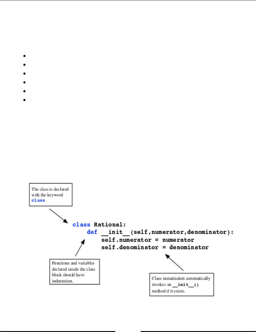
Classes
[ 168 ]
In mathematics, we often use the same operator symbol for completely different operations.
For instance, in 5+4 and sin + cos, the operator symbol + has different meanings. By using
the same symbol, one tries to express the similarities of mathematical operations. We have
introduced these terms from object-oriented programming by applying them to
mathematical examples:
Classes
Instance and instantiation
Inheritance
Methods
Attributes
Operator overloading
In this chapter, we will show how these concepts are used in Python.
Introduction to classes
We will illustrate the concept of classes with an example of rational numbers, that is,
numbers of the form q= qN ⁄ qD, where qN and qD are integers.
Figure 8.1: An example of a class declaration

Classes
[ 169 ]
We use rational numbers here only as an example for the class concept. For future work in
Python with rational numbers use the fractions module (refer to [6]).
Class syntax
The definition of a class is made by a block command with the class keyword, the name of
the class, and some statements in the block (refer to Figure 8.1):
class RationalNumber:
pass
An instance of this class (or in other words, an object of the type RationalNumber) is
created by
r = RationalNumber()
and a query type(a) returns the answer, <class'__main__.RationalNumber'>. If we
want to investigate whether an object is an instance of this class, we can use this:
if isinstance(a, RationalNumber):
print('Indeed it belongs to the class RationalNumber')
So far we've generated an object of the RationalNumber type, which has no data yet.
Furthermore, there are no methods defined to perform operations with these objects. This
will be the subject of the next sections.
The __init__ method
Now we provide our example class with some attributes; that is, we give it defining data. In
our case, this data will be the values of the denominator and the numerator. To this end, we
have to define a method, __init__, used to initialize the class with these values:
class RationalNumber:
def __init__(self, numerator, denominator):
self.numerator = numerator
self.denominator = denominator
Classes
[ 170 ]
Before we explain the special __init__ function, which we added to the class, we
demonstrate the instantiation of a RationalNumber object:
q = RationalNumber(10, 20) # Defines a new object
q.numerator # returns 10
q.denominator # returns 20
A new object of type RationalNumber is created by using the class name as if it was a
function. This statement does two things:
It first creates an empty object, q.
Then it applies the __init__ function to it; that is, q.__init__(10, 20) is
executed.
The first parameter of __init__ refers to the new object itself. On function call, this first
parameter is replaced by the object’s instance. This applies to all methods of the class and
not only to the special method __init__. The special role of this first parameter is reflected
by the convention to name it self. In the previous example, the __init__ function defines
two attributes of the new object, numerator and denominator.
Attributes and methods
One of the main reasons for working with classes is that objects can be grouped together
and bound to a common object. We saw this already when looking at rational numbers;
denominator and numerator are two objects which we bound to an instance of the
RationalNumber class. They are called attributes of the instance. The fact that an object is
an attribute of a class instance becomes apparent from the way they are referenced, which
we have used tacitly before:
<object>.attribute
Here are some examples of instantiation and attribute reference:
q = RationalNumber(3, 5) # instantiation
q.numerator # attribute access
q.denominator
a = array([1, 2]) # instantiation
a.shape
z = 5 + 4j # instantiation
z.imag

Classes
[ 171 ]
Once an instance is defined we can set, change or delete attributes of that particular
instance. The syntax is the same as for regular variables:
q = RationalNumber(3, 5)
r = RationalNumber(7, 3)
q.numerator = 17
del r.denominator
Changing or deleting an attribute may have undesired side effects, which might even
render the object useless. We will be learning more on this in the section Attributes that
depend on each other. As functions are objects too, we can also use functions as attributes;
they are called methods of the instance:
<object>.method(<arguments...>)
For example, let us add a method to the class RationalNumber that converts the number to
a float:
class RationalNumber:
...
def convert2float(self):
return float(self.numerator) / float(self.denominator)
Again, this method takes as its first (and only) argument, self, the reference to the object
itself. We use this method with a regular function call:
q = RationalNumber(10, 20) # Defines a new object
q.convert2float() # returns 0.5
This is equivalent to the following call:
RationalNumber.convert2float(q)
Note again that the object instance is inserted as the first argument of the function. This use
of the first argument explains the error message that would occur if this particular method
were used with additional arguments:
The q.convert2float(15) call provokes this error message:
TypeError: convert2float() takes exactly 1 argument (2 given)

Classes
[ 172 ]
The reason this does not work is that q.convert2float(15) is precisely equivalent to
RationalNumber.convert2float(q,15), which fails
because RationalNumber.convert2float takes only one argument.
Special methods
The special method __repr__ gives us the ability to define the way the object is
represented in a Python interpreter. For rational numbers, a possible definition of this
method could be as follows:
class RationalNumber:
...
def __repr__(self):
return '{} / {}'.format(self.numerator,self.denominator)
With this method defined, just typing q returns 10 / 20.
We would like to have a method that performs addition of two rational numbers. A first
attempt could result in a method like this:
class RationalNumber:
...
def add(self, other):
p1, q1 = self.numerator, self.denominator
if isinstance(other, int):
p2, q2 = other, 1
else:
p2, q2 = other.numerator, other.denominator
return RationalNumber(p1 * q2 + p2 * q1, q1 * q2)
A call to this method takes the following form:
q = RationalNumber(1, 2)
p = RationalNumber(1, 3)
q.add(p) # returns the RationalNumber for 5/6

Classes
[ 173 ]
It would be much nicer if we could write q + p instead. But so far, the plus sign is not
defined for the RationalNumber type. This is done by using the __add__ special method.
So, just renaming add to __add__ allows for using the plus sign for rational numbers:
q = RationalNumber(1, 2)
p = RationalNumber(1, 3)
q + p # RationalNumber(5, 6)
The expression q + p is in fact an alias for the expression q.__add__(p). In the table
(Table 8.1), you will find the special methods for binary operators, such as +, -, or *.
Operator Method Operator Method
+ __add__ += __iadd__
* __mul__ *= __imul__
- __sub__ -= __isub__
/ __truediv__ /= __itruediv__
// __floordiv__ //= __ifloordiv__
** __pow__
== __eq__ != __ne__
<= __le__ < __lt__
>= __ge__ > __gt__
() __call__ [] __getitem__
Table 8.1: Some Python operators & corresponding class methods, you can find the
complete list [31]
The implementation of those operators for a new class is called operator overloading.
Another example of operator overloading is a method for examining whether two rational
numbers are the same:
class RationalNumber:
...
def __eq__(self, other):
return self.denominator * other.numerator ==
self.numerator * other.denominator
It is used like this:
p = RationalNumber(1, 2) # instantiation
q = RationalNumber(2, 4) # instantiation
p == q # True

Classes
[ 174 ]
Operations between objects belonging to different classes need special care:
p = RationalNumber(1, 2) # instantiation
p + 5 # corresponds to p.__add__(5)
5 + p # returns an error
By default, the + operator invokes the left operand’s method, __add__. We programmed it
so that it allows both, objects of type int and objects of type RationalNumber. In the
statement 5 + p, the operands are commuted and the __add__ method of the build-in int
type is invoked. This method returns an error as it does not know how to handle rational
numbers. This case can be handled by the method __radd__, with which we will equip the
RationalNumber class now. The method __radd__ is called reverse addition.
Reverse operations
If operations like + are applied to two operands of different types, the corresponding
method (in this case, __add__) of the left operand is invoked first. If this raises an
exception, the reverse method (here, __radd__) of the right operand is called. If this
method does not exist, a TypeError exception is raised.
Consider an example of reverse operation. In order to enable the operation 5+p where p is
an instance of RationalNumber, we define this:
class RationalNumber:
....
def __radd__(self, other):
return self + other
Note that __radd__ interchanges the order of the arguments; self is the object of type
RationalNumber while other is the object that has to be converted.
Using a class instance together with brackets, ( , ) or [ , ] invokes a call to one of the special
methods __call__ or __getitem__, giving the instance the behavior of a function or of an
iterable (refer to the Table 8.1 for these and other special methods):
class Polynomial:
...
def __call__(self, x):
return self.eval(x)

Classes
[ 175 ]
Which now may be used as follows:
p = Polynomial(...)
p(3.) # value of p at 3.
The __getitem__ special method makes sense if the class provides an iterator (It is
recommended to refer section Iterators in Chapter 9, Iterating before you consider the
following example).
The recursion ui+1 = a1ui+ a0ui-1 is called a three–term recursion. It plays an important role in
applied mathematics, in particular in the construction of orthogonal polynomials. We can
set up a three-term recursion as a class in the following way:
import itertools
class Recursion3Term:
def __init__(self, a0, a1, u0, u1):
self.coeff = [a1, a0]
self.initial = [u1, u0]
def __iter__(self):
u1, u0 = self.initial
yield u0 # (see also Iterators section in Chapter 9)
yield u1
a1, a0 = self.coeff
while True :
u1, u0 = a1 * u1 + a0 * u0, u1
yield u1
def __getitem__(self, k):
return list(itertools.islice(self, k, k + 1))[0]
Here, the __iter__ method defines a generator object, which allows us to use an instance
of the class as an iterator:
r3 = Recursion3Term(-0.35, 1.2, 1, 1)
for i, r in enumerate(r3):
if i == 7:
print(r) # returns 0.194167
break
The __getitem__ method enables us to directly access the iterates as if r3 were a list:
r3[7] # returns 0.194167

Classes
[ 176 ]
Note that we used itertools.islice when coding the __getitem__ method (refer to
section Iterators of Chapter 9, Iterating, for more information). An example of the use of
__getitem__ together with slices and the function ogrid is given in the section Function
with two variables in Chapter 5, Advance Array Concepts.
Attributes that depend on each other
Attributes of an instance can be changed (or created) by simply assigning them a value.
However, if other attributes depend on the one just changed, it is desirable to change these
simultaneously:
Let us consider a class that defines an object for planar triangles from three given points. A
first attempt to set up such a class could be as follows:
class Triangle:
def __init__(self, A, B, C):
self.A = array(A)
self.B = array(B)
self.C = array(C)
self.a = self.C - self.B
self.b = self.C - self.A
self.c = self.B - self.A
def area(self):
return abs(cross(self.b, self.c)) / 2
An instance of this triangle is created by this:
tr = Triangle([0., 0.], [1., 0.], [0., 1.])
And its area is computed by this:
tr.area() # returns 0.5
If we change an attribute, say point B, the corresponding edges a and c are not automatically
updated and the computed area is wrong:
tr.B = [12., 0.]
tr.area() # still returns 0.5, should be 6 instead.
A remedy is to define a method that is executed when an attribute is changed; such a
method is called a setter method. Correspondingly, one might ask for a method that is
executed when a value of an attribute is requested; such a method is called a getter method.

Classes
[ 177 ]
The property function
The function property links an attribute to such a getter, setter, and deleter method. It
might also be used to assign a documentation string to an attribute:
attribute = property(fget = get_attr, fset = set_attr,
fdel = del_attr, doc = string)
We continue with the previous example with a setter method and consider
the Trinagle class again. If the following statement is included in Triangle
B = property(fget = get_B, fset = set_B, fdel = del_B, doc = ’The point B of
a triangle’)
a command
tr.B = <something>
invokes the setter method, set_B.
Let us modify the Triangle class:
class Triangle:
def __init__(self, A, B, C):
self._A = array(A)
self._B = array(B)
self._C = array(C)
self._a = self._C - self._B
self._b = self._C - self._A
self._c = self._B - self._A
def area(self):
return abs(cross(self._c, self._b)) / 2.
def set_B(self, B):
self._B = B
self._a = self._C - self._B
self._c = self._B - self._A
def get_B(self):
return self._B
def del_Pt(self):
raise Exception('A triangle point cannot be deleted')
B = property(fget = get_B, fset = set_B, fdel = del_Pt)
If the attribute B is changed, then the method set_B stores the new value in the internal
attribute _B and changes all depending attributes:
tr.B = [12., 0.]
tr.area() # returns 6.0

Classes
[ 178 ]
The way the deleter method is used here is to prevent deletion of attributes:
del tr.B # raises an exception
The use of an underscore as a prefix of attribute names is a convention used to indicate
attributes that are not designed to be accessed directly. They are intended to hold data for
attributes handled by setters and getters. These attributes are not private in the sense of
other programming languages; they are just not intended to be accessed directly.
Bound and unbound methods
We will now take a closer look at attributes that are methods. Let us consider an example:
class A:
def func(self,arg):
pass
A little inspection shows us how the nature of func changes after creating an instance:
A.func # <unbound method A.func>
instA = A() # we create an instance
instA.func # <bound method A.func of ... >
Calling, for example, A.func(3) would result in an error message such as this:
TypeError: func() missing 1 required positional argument: 'arg'
instA.func(3) is executed as expected. Upon creation of an instance, the func method is
bound to the instance. The self argument gets the instance assigned as its value. Binding a
method to an instance makes the method usable as a function. Before that, it is of no use.
Class methods, which we will consider later, are different in this aspect.
Class attributes
Attributes specified in the class declaration are called class attributes. Consider the
following example:
class Newton:
tol = 1e-8 # this is a class attribute
def __init__(self,f):
self.f = f # this is not a class attribute
....

Classes
[ 179 ]
Class attributes are useful for simulating default values and can be used if values have to be
reset:
N1 = Newton(f)
N2 = Newton(g)
Both instances have an attribute, tol, with the value initialized in the class definition:
N1.tol # 1e-8
N2.tol # 1e-8
Altering the class attribute automatically affects all the corresponding attributes of all
instances:
Newton.tol = 1e-10
N1.tol # 1e-10
N2.tol # 1e-10
Altering tol for one instance does not affect the other instance:
N2.tol = 1.e-4
N1.tol # still 1.e-10
But now N2.tol is detached from the class attribute. Changing Newton.tol no longer has
any effect on N2.tol:
Newton.tol = 1e-5 # now all instances of the Newton classes have 1e-5
N1.tol # 1.e-5
N2.tol # 1e-4 but not N2.
Class methods
We saw in the previous section on Bound and unbound methods how methods are either
bound to an instance of a class or remain in a state as unbound methods. Class methods are
different. They are always bound methods. They are bound to the class itself.
We will first describe the syntactic details and then give some examples to show what these
methods can be used for. To indicate that a method is a class method the decorator line
precedes the method definition:
@classmethod

Classes
[ 180 ]
While standard methods make a reference to an instance by the use of their first argument,
the first argument of a class method refers to the class itself. By convention the first
argument is called self for standard methods and cls for class methods.
Standard case:
class A:
def func(self,*args):
<...>
Class method case:
class B:
@classmethod
def func(cls,*args):
<...>
In practice, class methods may be useful for executing commands before an instance is
created, for instance, in a preprocessing step. See the following example:
In this example we show how class methods can be used to prepare data before creating an
instance:
class Polynomial:
def __init__(self, coeff):
self.coeff = array(coeff)
@classmethod
def by_points(cls, x, y):
degree = x.shape[0] - 1
coeff = polyfit(x, y, degree)
return cls(coeff)
def __eq__(self, other):
return allclose(self.coeff, other.coeff)
The class is designed so, that a polynomial object is created by specifying its coefficients.
Alternatively, the by_points class method allows us to define a polynomial by
interpolation points. We can transform the interpolation data to the polynomial coefficients
even when no instance of Polynomial is available:
p1 = Polynomial.by_points(array([0., 1.]), array([0., 1.]))
p2 = Polynomial([1., 0.])
print(p1 == p2) # prints True

Classes
[ 181 ]
Another example of a class method is presented in an example later in this chapter. In that
example, a class method is used to access information related to several (or all) instances
from this class.
Subclassing and inheritance
In this section, we will introduce some central concepts from object-oriented programming:
abstract classes, subclasses, and inheritance. To guide you through these concepts, we
consider another mathematical example: one-step methods for solving a differential
equation. The generic form of an ordinary initial value problem is
The data is the right-hand side function f, the initial value x0, and the interval of interest [t0,
te]. The solution of this problem is a function . A numerical algorithm gives this
solution as a vector u of discrete values ui being approximations to x(ti). Here,
are discretized values of the independent variable t, which in
physical models often represents time.
A one-step method constructs the solution values ui by the recursion steps:
Here, Φ is a step function that characterizes the individual methods (refer to [28]):
Explicit Euler:
Midpoint Rule:
Runge–Kutta 4:
with

Classes
[ 182 ]
What we did here is the typical way of describing a mathematical algorithm. We first
described a method by its idea, giving its steps in an abstract way. To actually use it, we
have to fill in the parameters of a concrete method, in this example, the function Φ. This is
also the way things are explained in object-oriented programming. First, we set up a class
with the abstract description of the method:
class OneStepMethod:
def __init__(self, f, x0, interval, N):
self.f = f
self.x0 = x0
self.interval = [t0, te] = interval
self.grid = linspace(t0, te, N)
self.h = (te - t0) / N
def generate(self):
ti, ui = self.grid[0], self.x0
yield ti, ui
for t in self.grid[1:]:
ui = ui + self.h * self.step(self.f, ui, ti)
ti = t
yield ti, ui
def solve(self):
self.solution = array(list(self.generate()))
def plot(self):
plot(self.solution[:, 0], self.solution[:, 1])
def step(self, f, u, t):
raise NotImplementedError()
This abstract class, with its methods, is used as a template for the individual methods:
class ExplicitEuler(OneStepMethod):
def step(self, f, u, t):
return f(u, t)
class MidPointRule(OneStepMethod):
def step(self, f, u, t):
return f(u + self.h / 2 * f(u, t), t + self.h / 2)
Note that in the class definitions, the name of the abstract class that we used as a template,
OneStepMethod, is given as an extra argument:
class ExplicitEuler(OneStepMethod)

Classes
[ 183 ]
That class is called the parent class. All methods and attributes of the parent class are
inherited by the subclasses as long as they are not overridden. They are overridden if they
are redefined in the subclass. The step method is redefined in the subclasses, while the
method generate is generic for the entire family and therefore inherited from the parent.
Before considering further details, we will demonstrate how these three classes can be used:
def f(x, t):
return -0.5 * x
euler = ExplicitEuler(f, 15., [0., 10.], 20)
euler.solve()
euler.plot()
hold(True)
midpoint = MidPointRule(f, 15., [0., 10.], 20)
midpoint.solve()
midpoint.plot()
You can avoid the repetition of common parameter lists by using the star operator (refer to
section Variable Number of Argument in Chapter 7, Functions for more details):
...
argument_list = [f, 15., [0., 10.], 20]
euler = ExplicitEuler(*argument_list)
...
midpoint = MidPointRule(*argument_list)
...
Note that the abstract class has never been used to create an instance. As the step method
was not completely defined, calling it raises an exception of type NotImplementedError.
Sometimes one has to access the methods or attributes of a parent class. This is done using
the command super. This is useful when the child class uses its own __init__ method in
order to extend the parent’s __init__:
For example let us assume that we want to give every solver class a string variable with the
solver’s name. To this end, we provide the solver with an __init__ method as it overrides
the parent’s __init__ method. In the case that both methods should be used, we have to
refer to the parent’s method by the command super:
class ExplicitEuler(OneStepMethod):
def __init__(self,*args, **kwargs):
self.name='Explicit Euler Method'
super(ExplicitEuler, self).__init__(*args,**kwargs)
def step(self, f, u, t):
return f(u, t)

Classes
[ 184 ]
Note that one could use the name of the parent class explicitly. The use of super instead
allows us to change the name of the parent class without having to change all the references
to the parent class.
Encapsulation
Sometimes the use of inheritance is impractical or even impossible. This motivates the use
of encapsulation. We will explain the concept of encapsulation by considering Python
functions, that is, objects of the Python type function, which we encapsulate in a new
class, Function, and provide with some relevant methods:
class Function:
def __init__(self, f):
self.f = f
def __call__(self, x):
return self.f(x)
def __add__(self, g):
def sum(x):
return self(x) + g(x)
return type(self)(sum)
def __mul__(self, g):
def prod(x):
return self.f(x) * g(x)
return type(self)(prod)
def __radd__(self, g):
return self + g
def __rmul__(self, g):
return self * g
Note that the __add__ and __mul__ operations should return an instance of the same class.
This is achieved by the return type(self)(sum) statement, which in this case is a more
general form of writing return Function(sum). We can now derive subclasses by
inheritance:
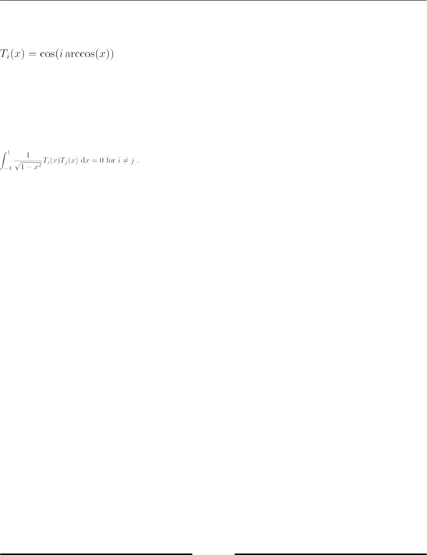
Classes
[ 185 ]
Consider as an example Chebyshev polynomials which can be computed in the interval
[1,-1] by:
.
We construct a Chebyshev polynomial as an instance of the Function class:
T5 = Function(lambda x: cos(5 * arccos(x)))
T6 = Function(lambda x: cos(6 * arccos(x)))
Chebyshev polynomials are orthogonal in the sense:
This can easily be checked using this construction:
import scipy.integrate as sci
weight = Function(lambda x: 1 / sqrt((1 - x ** 2)))
[integral, errorestimate] =
sci.quad(weight * T5 * T6, -1, 1) # (6.510878470473995e-17,
1.3237018925525037e-14)
Without encapsulation multiplying functions as simply as writing weight * T5 * T6
would not have been possible.
Classes as decorators
In section Function as decorators in Chapter 7, Functions , we saw how functions can be
modified by applying another function as a decorator. In previous examples, we saw how
classes can be made to behave as functions as long as they are provided with the __call__
method. We will use this here to show how classes can be used as decorators.

Classes
[ 186 ]
Let us assume that we want to change the behavior of some functions in such a way that
before the function is invoked, all input parameters are printed. This could be useful for
debugging purposes. We take this situation as an example to explain the use of a decorator
class:
class echo:
text = 'Input parameters of {name}n'+
'Positional parameters {args}n'+
'Keyword parameters {kwargs}n'
def __init__(self, f):
self.f = f
def __call__(self, *args, **kwargs):
print(self.text.format(name = self.f.__name__,
args = args, kwargs = kwargs))
return self.f(*args, **kwargs)
We use this class to decorate function definitions,
@echo
def line(m, b, x):
return m * x + b
and call the function as usual,
line(2., 5., 3.)
line(2., 5., x=3.)
On the second call, we obtain the following output:
Input parameters of line
Positional parameters (2.0, 5.0)
Keyword parameters {'x': 3.0}
11.0
This example shows that both classes and functions can be used as decorators. Classes allow
for more possibilities, as they can be used to collect data as well.
Indeed, we observe that:
Every decorated function creates a new instance of the decorator class.
Data collected by one instance can be saved and made accessible to another
instance by class attributes (refer section Attributes in Chapter 8, Classes).

Classes
[ 187 ]
The last point emphasizes the difference with function decorators. We show this now by a
decorator that counts function calls and stores the result in a dictionary with the function as
key.
In order to analyze the performance of algorithms, it might be useful to count the calls of
particular functions. We can get counter information without changing the function
definition. The code is a slight modification of an example given in [4] .
class CountCalls:
"""
Decorator that keeps track of the number of times
a function is called.
"""
instances = {}
def __init__(self, f):
self.f = f
self.numcalls = 0
self.instances[f] = self
def __call__(self, *args, **kwargs):
self.numcalls += 1
return self.f(*args, **kwargs)
@classmethod
def counts(cls):
"""
Return a dict of {function: # of calls} for all
registered functions.
"""
return dict([(f.__name__, cls.instances[f].numcalls)
for f in cls.instances])
Here, we use the class attribute CountCalls.instances to store the counters for each
individual instance. Let us see how this decorator works:
@CountCalls
def line(m, b, x):
return m * x + b
@CountCalls
def parabola(a, b, c, x):
return a * x ** 2 + b * x + c
line(3., -1., 1.)
parabola(4., 5., -1., 2.)
CountCalls.counts() # returns {'line': 1, 'parabola': 1}
parabola.numcalls # returns 1
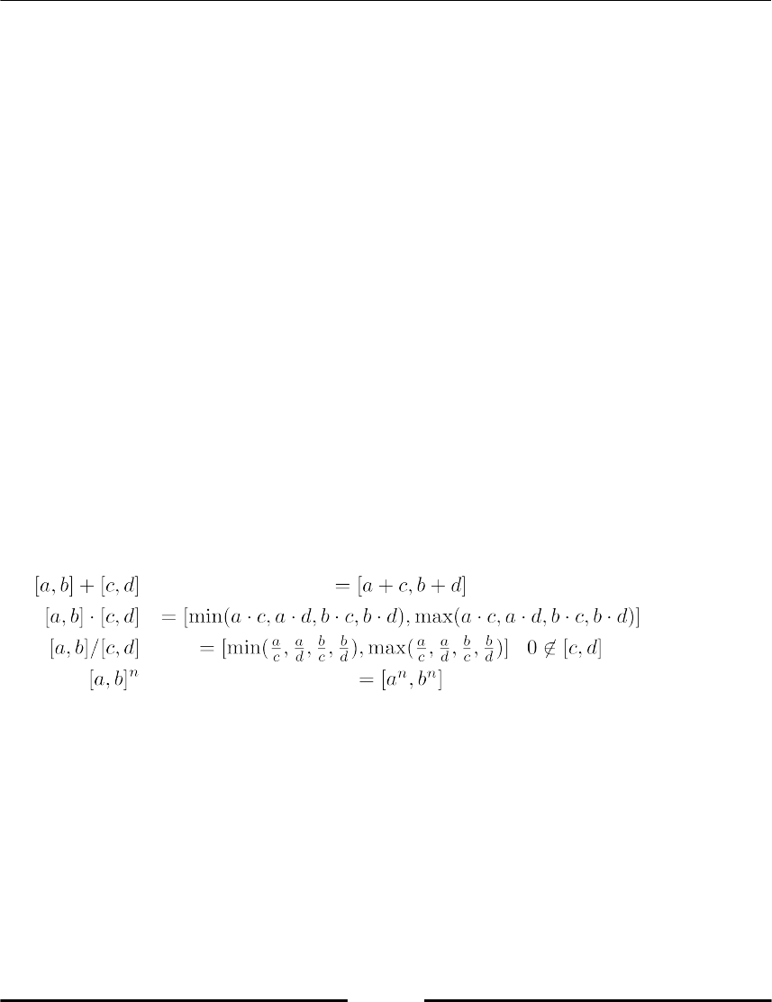
Classes
[ 188 ]
Summary
One of the most important programming concepts in modern computer science is object-
oriented programming. We learned in this chapter how to define objects as instances of
classes, which we provide with methods and attributes. The first parameter of methods,
usually denoted by self, plays an important and special role. You saw methods that can be
used to define basic operations such as + and * for your own classes.
While in other programming languages attributes and methods can be protected against
unintended use, Python allows a technique to hide attributes and access these hidden
attributes through special getter and setter methods. To this end, you met an important
function, property.
Exercises
Ex. 1 → Write a method simplify to the class RationalNumber. This method should
return the simplified version of the fraction as a tuple.
Ex. 2 → To provide results with confidence intervals a special calculus, so-called interval
arithmetic is introduced in numerical mathematics; (refer to [3, 14]). Define a class called
Interval and provide it with methods for addition, subtraction, division, multiplication,
and power (with positive integers only). These operations obey the following rules:
.
Provide this class with methods that allow operations of the type a + I, a I, I + a, I a, where I
is an interval and a an integer or float. Convert an integer or float to an interval [a,a] first.
(Hint: you may want to use function decorators for this; (refer to section Function as
decorators in Chapter 7, Functions). Furthermore, implement the __contains__ method,
which enables you to check if a given number belongs to the interval using the syntax x in
I for an object I of type Interval. Test your class by applying a polynomial f=lambda x:
25*x**2-4*x+1 to an interval.

Classes
[ 189 ]
Ex. 3 → Consider the example under section Classes as decorators. Extend this example to
obtain a function decorator that counts how often a certain function is called.
Ex. 4 → Compare the two ways to implement a method for reverse addition __radd__ in
the class RationalNumber: the one given in the example in section Special methods and the
one given here:
class RationalNumber:
....
def __radd__(self, other):
return other + self
Do you expect an error in this version? What is the error and how do you explain it? Test
your answer by executing:
q = RationalNumber(10, 15)
5 + q
Ex. 4 → Consider the decorator class CountCalls as in example in section Classes as
decorators. Provide this class with a method, reset, which sets the counters of all functions
in the dictionary, CountCalls.instances, to zero. What would happen if the dictionary
were replaced by an empty dictionary instead?
9
Iterating
In this chapter, we will present iteration using loops and iterators. We will show examples
of how this can be used with lists and generators. Iteration is one of the fundamental
operations a computer is useful for. Traditionally, iteration is achieved by a for loop. A for
loop is a repetition of a block of instructions a certain number of times. Inside the loop, one
has access to a loop variable, in which the iteration number is stored.
The Python idiom is slightly different. A for loop in Python is primarily designed to
exhaust a list, that is, to enumerate the elements of a list. The effect is similar to the
repetition effect just described if one uses a list containing the first n integers.
A for loop only needs one element of the list at a time. It is therefore desirable to use a for
loop with objects that are able to create those elements on demand, one at a time. This is
what iterators achieve in Python.
The for statement
The primary aim of the for statement is to traverse a list:
for s in ['a', 'b', 'c']:
print(s), # a b c
In this example, the loop variable s is successively assigned to one element of the list. Notice
that the loop variable is available after the loop has terminated. This may sometimes be
useful; refer, for instance, the example in section Controlling the flow inside the loop.

Iterating
[ 191 ]
One of the most frequent uses of a for loop is to repeat a given task a defined number of
times, using the function range (refer to section Lists of Chapter 1, Getting Started).
for iteration in range(n): # repeat the following code n times
...
If the purpose of a loop is to go through a list, many languages (including Python) offer the
following pattern:
for k in range(...):
...
element = my_list[k]
If the purpose of that code were to go through the list my_list, the preceding code
would not make it very clear. For this reason, a better way to express this is as follows:
for element in my_list:
...
It is now clear at first glance that the preceding piece of code goes through the my_list list.
Note that if you really need the index variable k, you may replace the preceding code by
this:
for k, element in enumerate(my_list):
...
The intent of this piece of code is to go through my_list while keeping the index variable k
available. A similar construction for arrays is the command ndenumerate.
Controlling the flow inside the loop
Sometimes it is necessary to jump out of the loop, or to go directly to the next loop iteration.
These two operations are performed by the break and continue commands. The
break keyword, as the name indicates, breaks the loop. Two situations can occur where the
loop breaks:
The loop is completely executed.
The loop is left before it was completely executed (break).

Iterating
[ 192 ]
For the first case, special actions can be defined in an else block, which is executed if the
whole list is traversed. This is useful in general if the purpose of the for loop is to find
something and stop. Examples might be searching for one element satisfying a
certain property inside a list. If such an element is not found, the else block is executed.
Here is a common usage in scientific computing. Quite often, we use an iterating algorithm
that is not guaranteed to succeed. In that case, it is preferable to use a (big) finite loop so
that the program does not get caught in an infinite loop. The for/else construct allows
such an implementation:
maxIteration = 10000
for iteration in range(maxIteration):
residual = compute() # some computation
if residual < tolerance:
break
else: # only executed if the for loop is not broken
raise Exception("The algorithm did not converge")
print("The algorithm converged in {} steps".format(iteration+1))
Iterators
A for loop is primarily used to traverse a list, but it picks the elements of the list one at a
time. In particular, there is no need to store the whole list in memory for the loop to work
properly. The mechanism that allows for loops to work without lists is that of iterators.
An iterable object produces objects (to be passed to a for loop). Such an object, obj, may be
used inside a for loop, as follows:
for element in obj:
...
The notion of iterator thus generalizes the idea of lists. The simplest example of an iterable
object is given by lists. The produced objects are simply the objects stored in the list:
L = ['A', 'B', 'C']
for element in L:
print(element)
An iterable object need not produce existing objects. The objects may, instead, be produced
on the fly.

Iterating
[ 193 ]
A typical iterable is the object returned by the function range. This function works as if it
would generate a list of integers, but instead, the successive integers are produced on the fly
when they are needed:
for iteration in range(100000000):
# Note: the 100000000 integers are not created at once
if iteration > 10:
break
If one really needs a list with all integers between 0 and 100,000,000, then it has to be formed
explicitly:
l=list(range(100000000))
Generators
You can create your own iterators using the yield keyword. For example, a generator for
odd numbers smaller than n can be defined:
def odd_numbers(n):
"generator for odd numbers less than n"
for k in range(n):
if k % 2 == 1:
yield k
Then you can use it as follows:
g = odd_numbers(10)
for k in g:
... # do something with k
Or even like this:
for k in odd_numbers(10):
... # do something with k

Iterating
[ 194 ]
Iterators are disposable
One salient feature of iterators is that they may be used only once. In order to use the
iterator again, you will have to create a new iterator object. Note that an iterable object is
able to create new iterators as many times as necessary. Let us examine the case of a list:
L = ['a', 'b', 'c']
iterator = iter(L)
list(iterator) # ['a', 'b', 'c']
list(iterator) # [] empty list, because the iterator is exhausted
new_iterator = iter(L) # new iterator, ready to be used
list(new_iterator) # ['a', 'b', 'c']
Each time a generator object is called, it creates a new iterator. Hence, when that iterator is
exhausted, one has to call the generator again to obtain a new iterator:
g = odd_numbers(10)
for k in g:
... # do something with k
# now the iterator is exhausted:
for k in g: # nothing will happen!!
...
# to loop through it again, create a new one:
g = odd_numbers(10)
for k in g:.
...
Iterator tools
Here are a couple of iterator tools that often come in very handy:
enumerate is used to enumerate another iterator. It produces a new iterator that
yields pairs (iteration, element), where iteration stores the index of the
iteration:
A = ['a', 'b', 'c']
for iteration, x in enumerate(A):
print(iteration, x)
# result: (0, 'a') (1, 'b') (2, 'c')

Iterating
[ 195 ]
reversed creates an iterator from a list by going through that list backwards.
Notice that this is different from creating a reversed list:
A = [0, 1, 2]
for elt in reversed(A):,
print(elt)
# result: 2 1 0
itertools.count is a possibly infinite iterator of integers:
for iteration in itertools.count():
if iteration > 100:
break # without this, the loop goes on forever
print("integer {}".format(iteration))
# prints the 100 first integer
intertools.islice truncates an iterator using the familiar slicing syntax;
refer to Chapter 3, Container Types. One application is creating a finite iterator
from an infinite one:
from itertools import count, islice
for iteration in islice(count(), 10):
# same effect as range(10)
...
For example, let's find some odd numbers by combining islice with an infinite generator.
First, we modify the generator for odd numbers so that it becomes an infinite generator:
def odd_numbers():
k=-1
while True:
k+=1
if k%2==1:
yield k
Then, we use it with islice to get a list of some odd numbers:
list(itertools.islice(odd_numbers(),10,30,8)) # returns [21, 37, 53]
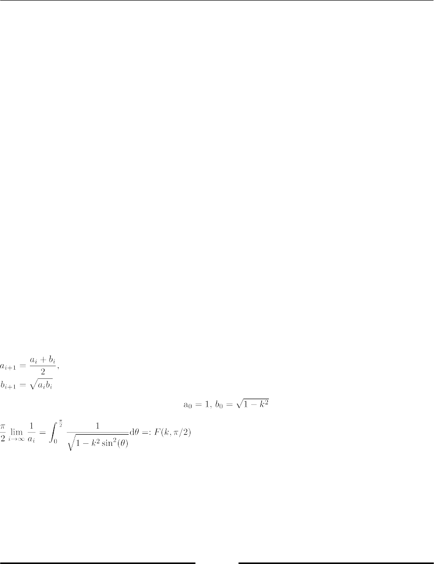
Iterating
[ 196 ]
Generators of recursive sequences
Assume that a sequence is given by an induction formula. For instance, consider the
Fibonacci sequence, defined by the recurrence formula: un = un-1 + un-2.
This sequence depends on two initial values, namely u0 and u1, although for the standard
Fibonacci sequence those numbers are taken as 0 and 1 respectively. A nifty way of
programming the generation of such a sequence is by using generators, as follows:
def fibonacci(u0, u1):
"""
Infinite generator of the Fibonacci sequence.
"""
yield u0
yield u1
while True:
u0, u1 = u1, u0+u1
yield u1
This may then be used, for instance, like this:
# sequence of the 100 first Fibonacci numbers:
list(itertools.islice(fibonacci(0, 1), 100))
Arithmetic geometric mean
The iteration based on iteratively computing arithmetic and geometric means is called
AGM iteration (refer to [1, p. 598] for more information):
It has the fascinating property that for :

Iterating
[ 197 ]
The integral on the right-hand side is called a complete elliptic integral of the first kind. We
now proceed to compute this elliptic integral. We use a generator to describe the iteration:
def arithmetic_geometric_mean(a, b):
"""
Generator for the arithmetic and geometric mean
a, b initial values
"""
while True: # infinite loop
a, b = (a+b)/2, sqrt(a*b)
yield a, b
As the sequence {ai} is convergent, the sequence {ci} defined by {ci} = (ai– bi)/2, converges to
zero – a fact that will be used to terminate the iteration in the program to compute the
elliptic integral:
def elliptic_integral(k, tolerance=1e-5):
"""
Compute an elliptic integral of the first kind.
"""
a_0, b_0 = 1., sqrt(1-k**2)
for a, b in arithmetic_geometric_mean(a_0, b_0):
if abs(a-b) < tolerance:
return pi/(2*a)
We have to make sure that the algorithm stops. Note that this code fully relies on the
mathematical statement that the arithmetic geometric mean iteration converges (fast). In
practical computing, we have to be careful while applying theoretical results, as they might
no longer be valid in limited-precision arithmetic. The right way to make the preceding
code safe is to use itertools.islice. The safe code is as follows (see the example under
the section Controlling the flow inside the loop for another typical usage of the for/else
statement):
from itertools import islice
def elliptic_integral(k, tolerance=1e-5, maxiter=100):
"""
Compute an elliptic integral of the first kind.
"""
a_0, b_0 = 1., sqrt(1-k**2)
for a, b in islice(arithmetic_geometric_mean(a_0, b_0),
maxiter):
if abs(a-b) < tolerance:
return pi/(2*a)
else:
raise Exception("Algorithm did not converge")
Iterating
[ 198 ]
As an application, elliptic integrals may be used to compute the period of a pendulum of
length L starting at an angle θ (refer to [18, p.114] for more information) using:
Using this formula, the period of the pendulum is easily obtained:
def pendulum_period(L, theta, g=9.81):
return 4*sqrt(L/g)*elliptic_integral(sin(theta/2))
Convergence acceleration
We give an example of application of generators for convergence acceleration. This
presentation follows closely the example given by Pramode C.E in Python Generator Tricks
(refer [9] for more information).
Note that a generator may take an other generator as an input parameter. For instance,
suppose that we have defined a generator that generates the elements of a converging
sequence. It is then possible to improve the convergence by an acceleration technique due to
Euler and Aitken, often called Aitken’s Δ2-method (Refer [33]). It transforms a sequence si
into another by defining
Both sequences have the same limit, but the sequence converges significantly faster. One
possible implementation is as follows:
def Euler_accelerate(sequence):
"""
Accelerate the iterator in the variable `sequence`.
"""
s0 = next(sequence) # Si
s1 = next(sequence) # Si+1
s2 = next(sequence) # Si+2
while True:
yield s0 - ((s1 - s0)**2)/(s2 - 2*s1 + s0)
s0, s1, s2 = s1, s2, next(sequence)
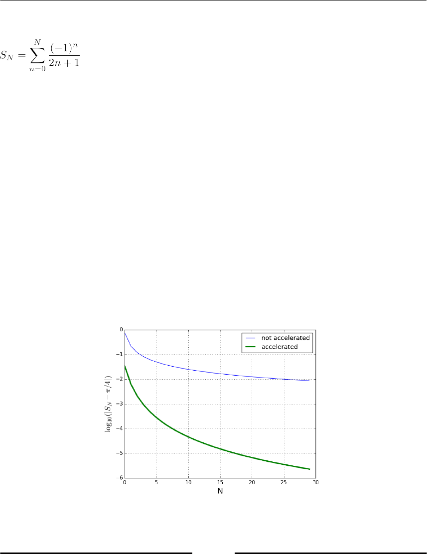
Iterating
[ 199 ]
As an example, we use the classical series:
It converges towards π/4. We implement this series as a generator in the following code:
def pi_series():
sum = 0.
j = 1
for i in itertools.cycle([1, -1]):
yield sum
sum += i/j
j += 2
We may now use the accelerated version of that sequence using this:
Euler_accelerate(pi_series())
Accordingly, the first N elements of that accelerated sequence are obtained with:
itertools.islice(Euler_accelerate(pi_series()), N)
For instance, the following figure (Figure 9.1) shows the convergence rate of the log of the
error for the standard version of the sequence defined by the above formula and its
accelerated version:
Figure 9.1: Comparison between the sequence defined and its accelerated version

Iterating
[ 200 ]
List filling patterns
In this section we will compare different ways to fill lists. They are different in
computational efficiency and also in code readability.
List filling with the append method
A ubiquitous programming pattern is to compute elements and store them in a list:
L = []
for k in range(n):
# call various functions here
# that compute "result"
L.append(result)
This approach has a number of disadvantages:
The number of iterations is decided in advance. If there is a break instruction,
then the preceding code takes care of both generating values and deciding when
to stop. This is not desirable and lacks flexibility.
It makes the assumption that the user wants the whole history of the
computation, for all the iterations. Suppose we are only interested in the sum of
all the computed values. If there are many computed values, it does not make
sense to store them, as it is much more efficient to add them one at a time.
List from iterators
Iterators provide us with an elegant solution to problems discussed previously:
def result_iterator():
for k in itertools.count(): # infinite iterator
# call various functions here
# that compute "result"
...
yield result
Iterating
[ 201 ]
With iterators, we separate the task of generating the computed values without bothering
about the stopping condition or about the storage. If the user of that code wants to store the
n first values, it is easily done using the list constructor:
L = list(itertools.islice(result_iterator(), n)) # no append needed!
If the user wants the sum of the first n generated values, this construction is recommended:
# make sure that you do not use scipy.sum here
s = sum(itertools.islice(result_iterator(), n))
What we did here was separating the generation of elements on one hand, and storing those
elements on the other.
If the purpose is really to build a list, and when the result at each step does not depend on
previously computed elements, one may use the list comprehension syntax (refer to section
List of Chapter 3, Container Types, for more information):
L = [some_function(k) for k in range(n)]
When iteratively computing values that depend on the previously computed values, list
comprehensions cannot help.
Storing generated values
Using iterators to fill out lists will work nicely most of the time, but there are complications
to this pattern when the algorithm computing the new values is liable to throw an
exception; if the iterator raises an exception along the way, the list will not be available! The
following example illustrates this problem.
Suppose we generate the sequence defined recursively by . This sequence
quickly diverges to infinity if the initial data u0 is greater than one. Let us generate it with a
generator:
import itertools
def power_sequence(u0):
u = u0
while True:
yield u
u = u**2

Iterating
[ 202 ]
If you try to obtain the first 20 elements of the sequence (initialized by u0 = 2) by executing,
list(itertools.islice(power_sequence(2.), 20))
an exception will be raised and no list will be available, not even the list of elements before
the exception was raised. There is currently no way to obtain a partially filled list from a
possibly faulty generator. The only way around is to use the append method wrapped in an
exception-catching block (refer to section Exceptions in Chapter 10, Error Handling, for more
details):
generator = power_sequence(2.)
L = []
for iteration in range(20):
try:
L.append(next(generator))
except Exception:
...
When iterators behave as lists
Some list operations also work on iterators. We will now examine the equivalents of list
comprehensions and list zipping (refer to section List of Chapter 3, Container Types, for more
details).
Generator expression
There is an equivalent of list comprehension for generators. Such a construction is called a
generator expression:
g = (n for n in range(1000) if not n % 100)
# generator for 100, 200, ... , 900
This is useful in particular for computing sums or products because those operations are
incremental; they only need one element at a time:
sum(n for n in range(1000) if not n % 100) # returns 4500
In that code, you notice that the sum function is given one argument, which is a generator
expression. Note that Python syntax allows us to omit the enclosing parentheses of
generators when a generator is used as the only argument of a function.
Iterating
[ 203 ]
Let us compute the Riemann zeta function ζ, whose expression is
With a generator expression, we may compute a partial sum of this series in one line:
sum(1/n**s for n in itertools.islice(itertools.count(1), N))
Note that we could also have defined a generator of the sequence 1 ⁄ ns as follows:
def generate_zeta(s):
for n in itertools.count(1):
yield 1/n**s
Then we simply obtain the sum of the first N terms using:
def zeta(N, s):
# make sure that you do not use the scipy.sum here
return sum(itertools.islice(generate_zeta(s), N))
We point out that we used this way of computing the zeta (ζ) function as a demonstration
of the use of generators in an elegant way. It is certainly not the most accurate and
computationally efficient way to evaluate this function.
Zipping iterators
We saw in section List, Chapter 3, Container Types, that it is possible to create a list out of
two by zipping them together. The same operation exists for iterators:
xg = x_iterator() # some iterator
yg = y_iterator() # another iterator
for x, y in zip(xg, yg):
print(x, y)
The zipped iterator stops as soon as one of the iterators is exhausted. This is the same
behavior as for a zip operation on lists.

Iterating
[ 204 ]
Iterator objects
As we mentioned earlier, a for loop only needs an iterable object. Lists, in particular, are
iterable. This means that a list is able to create an iterator from its contents. In fact, this is
true for any object (not only lists): any object may be made iterable.
This is achieved via the __iter__ method, which should return an iterator. Here we give
an example where the __iter__ method is a generator:
class OdeStore:
"""
Class to store results of ode computations
"""
def __init__(self, data):
"data is a list of the form [[t0, u0], [t1, u1],...]"
self.data = data
def __iter__(self):
"By default, we iterate on the values u0, u1,..."
for t, u in self.data:
yield u
store = OdeStore([[0, 1], [0.1, 1.1], [0.2, 1.3]])
for u in store:
print(u)
# result: 1, 1.1, 1.3
list(store) # [1, 1.1, 1.3]
If you try to use the features of an iterator with an object that is not iterable, an exception
will be raised:
>>> list(3)
TypeError: 'int' object is not iterable
In this example, the list function tries to iterate through the object 3 by calling the
__iter__ method. But this method is not implemented for integers and thus the exception
is raised. The same would happen if we tried to cycle through a non-iterable object:
>>> for iteration in 3: pass
TypeError: 'int' object is not iterable

Iterating
[ 205 ]
Infinite iterations
Infinite iterations are obtained either with an infinite iterator, with a while loop, or by
recursion. Obviously, in practical cases, some condition stops the iteration. The difference
with finite iterations is that it is impossible to say by a cursory examination of the code,
whether the iteration will stop or not.
The while loop
The while loop may be used to repeat a code block until a condition is fulfilled:
while condition:
<code>
A while loop is equivalent to the following code:
for iteration in itertools.count():
if not condition:
break
<code>
So a while loop is equivalent to an infinite iterator, which might be stopped if a condition is
fulfilled. The danger of such a construction is obvious: the code may be trapped in an
infinite loop if the condition is never fulfilled.
The problem in scientific computing is that one is not always sure that an algorithm will
converge. Newton iteration, for instance, might not converge at all. If that algorithm were
implemented inside a while loop, the corresponding code would be trapped in an infinite
loop for some choices of initial conditions.
We therefore give an advice that finite iterators are often better suited for such a task. The
following construction replaces, often advantageously, the use of a while loop:
maxit = 100
for nb_iterations in range(max_it):
...
else:
raise Exception("No convergence in {} iterations".format(maxit))
The first advantage is that the code is guaranteed to execute in a finite time no matter what
happens. The second advantage is that the variable nb_iterations contains the number of
iterations that was necessary for the algorithm to converge.

Iterating
[ 206 ]
Recursion
A recursion occurs when a function calls itself (refer to section Recursive Function in Chapter
7, Functions).
When doing recursions, it is the recursion depth, that is the number of iterations, which
brings your computer to its limits. We demonstrate this here by considering a simple
recursion, which actually contains no computations at all. It assigns to the iterates only the
value zero:
def f(N):
if N == 0:
return 0
return f(N-1)
Depending on your system, this program may choke for N ≥ 10000 (too much memory is
used). The result is that the Python interpreter crashes without further exception. Python
provides a mechanism to raise an exception when a too high recursion depth is detected.
This maximum recursion depth may be changed by executing:
import sys
sys.setrecursionlimit(1000)
The actual value of the recursion limit can be obtained by sys.getrecursionlimit().
Be aware though, that choosing too high a number may imperil the stability of your code,
since Python might crash before that maximum depth is reached. It is therefore often wise
to leave the recursion limit as it is.
By comparison, the following, non recursive, program runs ten of millions of iterations
without any problem:
for iteration in range(10000000):
pass
We advocate that, if possible, recursion should be avoided in Python. This applies
obviously only if there is an appropriate alternative iterative algorithm available. The first
reason is that a recursion of depth N involves N function calls at the same time, which
might result in a significant overhead. The second reason is that it is an infinite iteration,
that is, it is difficult to give an upper bound to the number of steps necessary before the
recursion is over.
Note that in some very special cases (tree traversal) recursion is unavoidable. Besides, in
some cases (with small recursion depths) recursive programs might be preferred due to
readability.
Iterating
[ 207 ]
Summary
In this chapter, we studied iterators, a programming construct very near to a mathematical
description of iterative methods. You saw the yield keyword and met finite and infinite
iterators.
We showed that an iterator can be exhausted. More special aspects such as iterator
comprehension and recursive iterators were introduced and demonstrated with the help of
examples.
Exercises
Ex. 1 → Compute the value of the sum:
Ex. 2 → Create a generator that computes the sequence defined by the relation:
Ex. 3 → Generate all the even numbers.
Ex. 4 → Let . In calculus, it is shown that . Determine experimentally
the smallest number n such that . Use a generator for this task.
Ex. 5 → Generate all prime numbers less than a given integer. Use the algorithm called Sieve
of Eratosthenes.
Ex. 6 → Solving the differential equation by applying the explicit Euler method
results in the recursion:
Write a generator that computes the solution values un for a given initial value u0 and for a
given value of the time step h.
Iterating
[ 208 ]
Ex. 7 → Compute π using the formula:
The integral can be approximated using the composite trapezoidal rule, that is, by this
formula:
where .
Program a generator for the values yi = f(xi) and evaluate the formula by summing one term
after the other. Compare your results with the quad function of SciPy.
Ex. 8 → Let x = [1, 2, 3] and y = [-1, -2, -3]. What is the effect of the code zip(*zip(x, y))?
Explain how it works.
Ex. 9 → Complete elliptic integrals can be computed by the function
scipy.special.ellipk. Write a function, which counts the number of iterations needed
with the AGM iteration until the result coincides up to a given tolerance (note that the
input parameter m in ellipk corresponds to k2 in the definition in the section Arithmetic
geometric mean) .
Ex. 10 → Consider the sequence defined by:
It converges monotonically to zero: E1 >E2 > . . . > 0. By integration by parts, one can show
that the sequence En fulfills the following recursion:
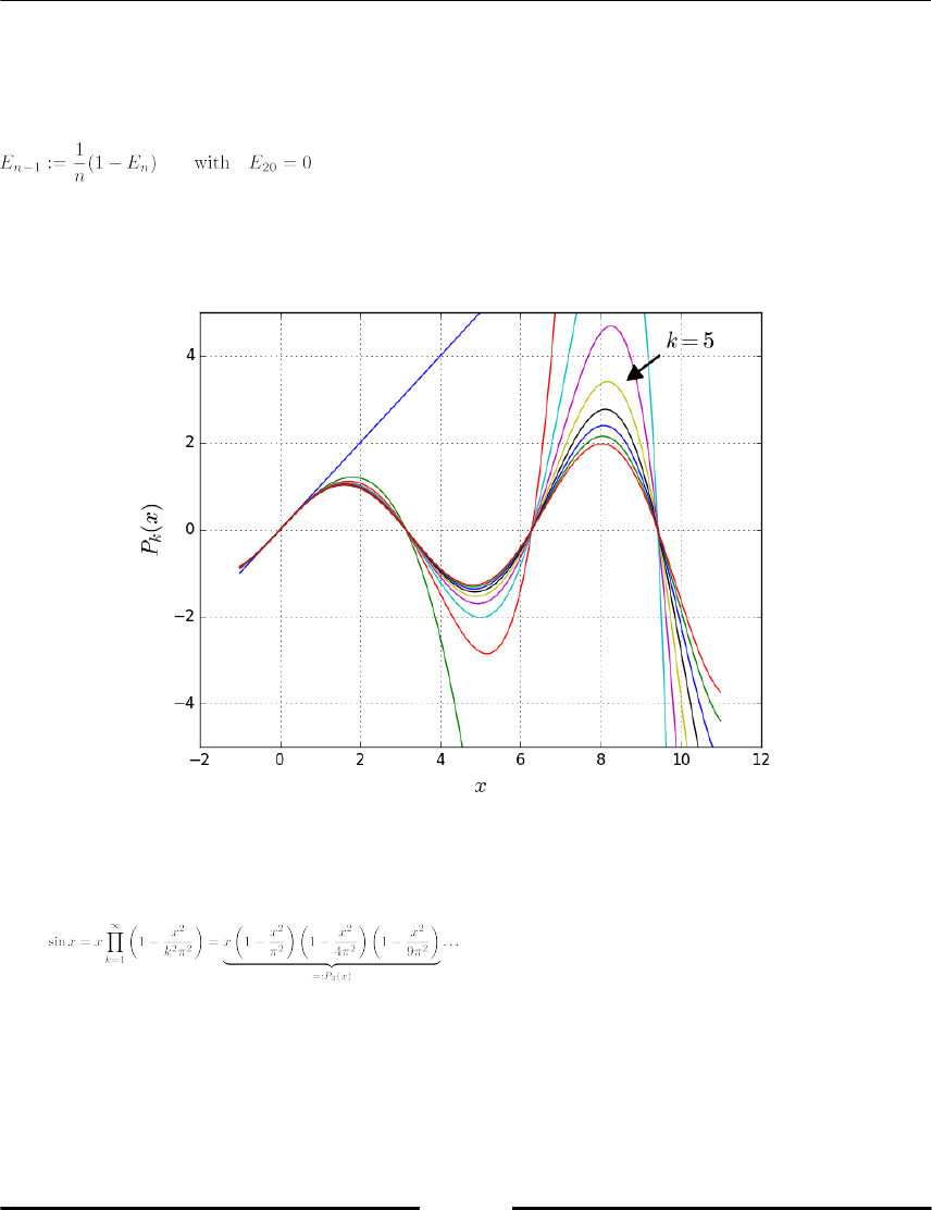
Iterating
[ 209 ]
Compute the first 20 terms of the recursion by using an appropriate generator and compare
the results with those obtained by numerical integration with scipy.integrate.quad. Do
the same by reversing the recursion:
Use the exp function to evaluate the exponential function. What do you observe? Do you
have an explanation? (refer to [29])
Figure 9.2: A convergence study of functions approximating to sin(x)
Ex. 11 → The sine-function can be expressed due to Euler as
Write a generator that generates the function values Pk(x). Set
x=linspace(-1,3.5*pi,200) and demonstrate graphically how good
Pk(x) approximates sin for increasing k. In previous figure (Figure 9.2), the possible result is
shown (refer to [11, Th. 5.2, p. 65]).
10
Error Handling
In this chapter, we will cover errors, exceptions, and how to find and fix them. Handling
exceptions is an important part of writing reliable and usable code. We will introduce the
basic built-in exceptions and show how to use and treat exceptions. We'll introduce
debugging and show you how to use the built-in Python debugger.
What are exceptions?
One error programmers (even experienced ones) find is when code has incorrect syntax,
meaning that the code instructions are not correctly formatted.
Consider an example of Syntax error:
>>> for i in range(10)
File “<stdin>”, line 1
for i in range(10)
^
SyntaxError: invalid syntax
The error occurs because of a missing colon at the end of the for declaration. This is an
example of an exception being raised. In the case of SyntaxError, it tells the programmer
that the code has incorrect syntax and also prints the line where the error occurred, with an
arrow pointing to where in that line the problem is.

Error Handling
[ 211 ]
Exceptions in Python are derived (inherited) from a base class called Exception. Python
comes with a number of built-in exceptions. Some common exception types are listed in
Table 10.1, (for full list of built-in exceptions refer to [38]).
Here are two common examples of exceptions. As you might expect, ZeroDivisionError
is raised when you try to divide by zero.
def f(x):
return 1/x
>>> f(2.5)
0.4
>>> f(0)
Traceback (most recent call last):
File "<stdin>", line 1, in <module>
File "exception_tests.py", line 3, in f
return 1/x
ZeroDivisionError: integer division or modulo by zero
Exception Description
IndexError Index is out of bounds, for example, v[10] when v only has 5 elements
KeyError A reference to an undefined dictionary key
NameError A name not found, for example, an undefined variable
LinAlgError Errors in the linalg module, for example, when solving a system with a
singular matrix
ValueError Incompatible data value, for example, when using dot with incompatible
arrays
IOError I/O operation fails, for example, “file not found”
ImportError A module or name is not found on import
Table10.1: Some frequently used built-in exceptions and their meaning
A division with zero raises ZeroDivisionError and prints out the file, line, and function
name where the error occurred.

Error Handling
[ 212 ]
As we have seen before, arrays can only contain elements of the same data type. If you try
to assign a value of an incompatible type, a ValueError is raised. An example, of a value
error:
>>> a = arange(8.0)
>>> a
array([ 0., 1., 2., 3., 4., 5., 6., 7.])
>>> a[3] = 'string'
Traceback (most recent call last):
File "<stdin>", line 1, in <module>
ValueError: could not convert string to float: string
Here, ValueError is raised because the array contains floats and an element cannot be
assigned a string value.
Basic principles
Let's look at the basic principles on how to use exceptions by raising them with raise
and catching them with try statements.
Raising exceptions
Creating an error is referred to as raising an exception. You saw some examples of
exceptions in the previous section. You can also define your own exceptions, of a
predefined type or type-less. Raising an exception is done with the command like this:
raise Exception("Something went wrong")
It might be tempting to print out error messages when something goes wrong, for example,
like this:
print("The algorithm did not converge.")
This is not recommended for a number of reasons. Firstly, printouts are easy to miss,
especially if the message is buried in many other messages being printed to your console.
Secondly, and more importantly, it renders your code unusable by other code. The calling
code will have no way of knowing that an error occurred and therefore have no way of
taking care of it.

Error Handling
[ 213 ]
For these reasons, it is always better to raise an exception instead. Exceptions should always
contain a descriptive message, for example:
raise Exception("The algorithm did not converge.")
This message will stand out clearly for the user. It also gives the opportunity for the calling
code to know that an error occurred, and to possibly find a remedy.
Here is a typical example of checking the input inside a function to make sure it is usable
before continuing. For an example, a simple check for negative values and the correct data
type ensures the intended input of a function to compute factorials:
def factorial(n):
if not (n >=0 and isinstance(n,(int,int32,int64))):
raise ValueError("A positive integer is expected")
...
The user of the function will immediately know what the error is, if an incorrect input is
given, and it is the user's responsibility to handle the exception. Note the use of the
exception name when raising a predefined exception type, in this case ValueError
followed by the message. By specifying the type of the exception, the calling code can
decide to handle errors differently depending on what type of error is raised.
Summing up, it is always better to raise exceptions than to print error messages.
Catching exceptions
Dealing with an exception is referred to as catching an exception. Checking for exceptions is
done with the try and except commands.
An exception stops the program execution flow and looks for the closest try enclosing
block. If the exception is not caught, the program unit is left and it continues searching for
the next enclosing try block in a program unit higher up in the calling stack. If no block is
found and the exception is not handled, execution stops entirely; the standard traceback
information is displayed.

Error Handling
[ 214 ]
Let's look at an example for the try statement:
try:
<some code that might raise an exception>
except ValueError:
print("Oops, a ValueError occurred")
In this case, if the code inside the try block raises an error of type ValueError, the
exception will be caught and the message in the except block printed. If no exception
occurs inside the try block, the except block is skipped entirely and execution continues.
The except statement can catch multiple exceptions. This is done by simply grouping them
in a tuple, like this:
except (RuntimeError, ValueError, IOError):
The try block can also have multiple except statements. This makes it possible to handle
exceptions differently depending on the type. Let's see an example of multiple exception
types:
try:
f = open('data.txt', 'r')
data = f.readline()
value = float(data)
except OSError as oe:
print("{}: {}".format(oe.strerror, oe.filename))
except ValueError:
print("Could not convert data to float.")
Here an OSError will be caught if, for example, the file does not exist; and a ValueError
will be caught if, for example, the data in the first line of the file is not compatible with the
float data type.
In this example we assigned the OSError to a variable oe by the keyword as. This allows to
access more details when handling this exception. Here we printed the error string
oe.strerror and the name of the related file oe.filename. Each error type can have its
own set of variables depending on the type. If the file does not exist, in the preceding
example, the message will be:
I/O error(2): No such file or directory

Error Handling
[ 215 ]
On the other hand, if the file exists but you don’t have permission to open it, the message
will be:
I/O error(13): Permission denied
This is a useful way to format the output when catching exceptions.
The try - except combination can be extended with optional else and finally blocks.
An example of using else can be seen in section Testing the bisection algorithm of Chapter
13, Testing. Combining try with finally gives a useful construction when cleanup work
needs to happen at the end:
An example for making sure a file is closed properly:
try:
f = open('data.txt', 'r')
# some function that does something with the file
process_file_data(f)
except:
...
finally:
f.close()
This will make sure that the file is closed at the end no matter what exceptions are thrown
while processing the file data. Exceptions that are not handled inside the try statement are
saved and raised after the finally block. This combination is used in the with statement;
see section Context Managers — the with statement.
User-defined exceptions
Besides the built-in Python exceptions, it is also possible to define your own exceptions.
Such user-defined exceptions should inherit from the Exception base class. This can be
useful when you define your own classes like the polynomial class in section Polynomials of
Chapter 14, Comprehensive Examples.
Take a look at this small example of a simple user-defined exception:
class MyError(Exception):
def __init__(self, expr):
self.expr = expr
def __str__(self):
return str(self.expr)
try:

Error Handling
[ 216 ]
x = random.rand()
if x < 0.5:
raise MyError(x)
except MyError as e:
print("Random number too small", e.expr)
else:
print(x)
A random number is generated. If the number is below 0.5, an exception is thrown and a
message that the value is too small is printed. If no exception is raised, the number is
printed.
In this example, you also saw a case of using else in a try statement. The block under
else will be executed if no exception occurs.
It is recommended that you define your exceptions with names that end in Error, like the
naming of the standard built-in exceptions.
Context managers — the with statement
There is a very useful construction in Python for simplifying exception handling when
working with contexts, such as files or databases. The statement encapsulates the try ...
finally structure in one simple command. Here is an example of using with to read a file:
with open('data.txt', 'r') as f:
process_file_data(f)
This will try to open the file, run the specified operations on the file (for example, reading),
and close the file. If anything goes wrong during the execution of process_file_data, the
file is closed properly and then the exception is raised. This is equivalent to:
f = open('data.txt', 'r')
try:
# some function that does something with the file
process_file_data(f)
except:
...
finally:
f.close()
We will use this option in section File handling of Chapter 12, Input and Output, when
reading and writing files.

Error Handling
[ 217 ]
The preceding file reading example is an example of using context managers. Context
managers are Python objects with two special methods, _ _enter_ _ and _ _exit_ _.
Any object of a class that implements these two methods can be used as a context manager.
In this example, the file object f is a context manager as there are f._ _enter_ _ and f._
_exit_ _ methods.
The _ _enter_ _ method should implement the initialization instructions, for example,
opening a file or a database connection. If this method has a return statement, the returned
object is accessed using the as construct. Otherwise, the as keyword is omitted. The _
_exit_ _ method contains the cleanup instructions, for example, closing a file or
committing transactions and closing a database connection. For more explanations and an
example of a self-written context manager, see the section Timing with a context manager of
Chapter 13, Testing.
There are NumPy functions that can be used as context managers. For example, the load
function supports context manager for some file formats. NumPy's function errstate
can be used as a context manager to specify floating-point error handling behavior within a
block of code.
Here is an example of working with errstate and a context manager:
import numpy as np # note, sqrt in NumPy and SciPy
# behave differently in that example
with errstate(invalid='ignore'):
print(np.sqrt(-1)) # prints 'nan'
with errstate(invalid='warn'):
print(np.sqrt(-1)) # prints 'nan' and
# 'RuntimeWarning: invalid value encountered in sqrt'
with errstate(invalid='raise'):
print(np.sqrt(-1)) # prints nothing and raises FloatingPointError
Refer section Infinite and Not a Number of Chapter 2, Variables and Basic Types, for more
details on this example and section Timing with a context manager of Chapter 13, Testing for
another example.

Error Handling
[ 218 ]
Finding Errors: Debugging
Errors in software code are sometimes referred to as bugs. Debugging is the process of
finding and fixing bugs in code. This process can be performed at varying degrees of
sophistication. The most efficient way is to use a tool called debugger. Having unittests in
place is a good way to identify errors early, refer section Using unittest of Chapter 13,
Testing. When it is not obvious where or what the problem is, a debugger is very useful.
Bugs
There are typically two kinds of bugs:
An exception is raised and not caught.
The code does not function properly.
The first case is usually easier to fix. The second can be more difficult as the problem can be
a faulty idea or solution, a faulty implementation, or a combination of the two.
We are only concerned with the first case in what follows, but the same tools can be used to
help find why the code does not do what it is supposed to.
The stack
When an exception is raised, you see the call stack. The call stack contains the trace of all the
functions that called the code where the exception was raised.
A simple stack example:
def f():
g()
def g():
h()
def h():
1//0
f()

Error Handling
[ 219 ]
The stack in this case is f, g, and h. The output generated by running this piece of code
looks like this:
Traceback (most recent call last):
File "stack_example.py", line 11, in <module>
f()
File "stack_example.py", line 3, in f
g()
File "stack_example.py", line 6, in g
h() File "stack_example.py", line 9, in h
1//0
ZeroDivisionError: integer division or modulo by zero
The error is printed. The sequence of functions leading up to the error is shown. The
function f on line 11 was called, which in turn called g and then h. This caused the
ZeroDivisionError.
A stack trace reports on the active stack certain point in the execution of a program. A stack
trace lets you track the sequence of functions called up to a given point. Often this is after an
uncaught exception has been raised. This is sometimes called post-mortem analysis, and the
stack trace point is then the place where the exception occurred. Another option is to invoke
a stack trace manually to analyze a piece of code where you suspect there is an error,
perhaps before the exception occurs.
The Python debugger
Python comes with its own built-in debugger called pdb. Some development environments
come with the debugger integrated. The following process still holds in most of these cases.
The easiest way to use the debugger is to enable stack tracing at the point in your code that
you want to investigate. Here is a simple example of triggering the debugger based on the
example mentioned in section Return values of Chapter 7, Functions:
import pdb
def complex_to_polar(z):
pdb.set_trace()
r = sqrt(z.real ** 2 + z.imag ** 2)
phi = arctan2(z.imag, z.real)
return (r,phi)
z = 3 + 5j
r,phi = complex_to_polar(z)
print(r,phi)

Error Handling
[ 220 ]
The pdb.set_trace() command starts the debugger and enables tracing of subsequent
commands. The preceding code will show this:
> debugging_example.py(7)complex_to_polar()
-> r = sqrt(z.real ** 2 + z.imag ** 2)
(Pdb)
The debugger prompt is indicated with (Pdb). The debugger stops the program execution
and gives you a prompt that lets you inspect variables, modify variables, step through
commands, and so on.
The current line is printed at each step, so you can follow where you are and what will
happen next. Stepping through commands is done with the command n (next), like this:
> debugging_example.py(7)complex_to_polar()
-> r = sqrt(z.real ** 2 + z.imag ** 2)
(Pdb) n
> debugging_example.py(8)complex_to_polar()
-> phi = arctan2(z.imag, z.real)
(Pdb) n
> debugging_example.py(9)complex_to_polar()
-> return (r,phi)
(Pdb)
...
The command n (next) will continue to the next line and print the line. If you need to see
more than one line at the time, the list command l (list) shows the current line with
surrounding code:
Listing surrounding code in the debugger:
> debugging_example.py(7)complex_to_polar()
-> r = sqrt(z.real ** 2 + z.imag ** 2)
(Pdb) l
2
3 import pdb
4
5 def complex_to_polar(z):
6 pdb.set_trace()
7 -> r = sqrt(z.real ** 2 + z.imag ** 2)
8 phi = arctan2(z.imag, z.real)
9 return (r,phi)
10
11 z = 3 + 5j
12 r,phi = complex_to_polar(z)
(Pdb)

Error Handling
[ 221 ]
Inspection of variables can be done by printing their values to the console using the
command p (print) followed by the variable name. An example of printing variables:
> debugging_example.py(7)complex_to_polar()
-> r = sqrt(z.real ** 2 + z.imag ** 2)
(Pdb) p z
(3+5j) (Pdb) n
> debugging_example.py(8)complex_to_polar()
-> phi = arctan2(z.imag, z.real)
(Pdb) p r
5.8309518948453007
(Pdb) c
(5.8309518948453007, 1.0303768265243125)
The p (print) command will print the variable; command c (continue) continues execution.
Changing a variable in mid-execution is useful. Simply assign the new value at the
debugger prompt and step or continue the execution.
An example of changing variables:
> debugging_example.py(7)complex_to_polar()
-> r = sqrt(z.real ** 2 + z.imag ** 2)
(Pdb) z = 2j
(Pdb) z
2j
(Pdb) c
(2.0, 1.5707963267948966)
Here the variable z is assigned a new value to be used throughout the remaining code. Note
that the final printout has changed.
Overview – debug commands
In Table 10.2, the most common debug commands are shown. For a full listing and
description of commands, (see the documentation [25] for more information). Note that
any Python command also works, for example, assigning values to variables.

Error Handling
[ 222 ]
Short variable names
If you want to inspect a variable with a name that coincides with any of
the debugger's short commands, for example, h, you must use !h to
display the variable.
Command Action
hHelp (without arguments, it prints available commands)
lList the code around the current line
qQuit (exits the debugger and the execution stops)
cContinue execution
rContinue execution until the current function returns
nContinue execution until the next line
p <expression> Evaluate and print the expression in the current context
Table10.2: The most common debug commands for the debugger.
Debugging in IPython
IPython comes with a version of the debugger called ipdb. At the time of writing this book,
the differences are very minor but this may change.
There is a command in IPython that automatically turns on the debugger in case of an
exception. This is very useful when experimenting with new ideas or code. An example of
how to automatically turn on the debugger in IPython:
In [1]: %pdb # this is a so - called IPython magic command
Automatic pdb calling has been turned ON
In [2]: a = 10
In [3]: b = 0
In [4]: c = a/b
___________________________________________________________________
ZeroDivisionError Traceback (most recent call last)
<ipython-input-4-72278c42f391> in <module>()
—-> 1 c = a/b
ZeroDivisionError: integer division or modulo by zero
> <ipython-input-4-72278c42f391>(1)<module>()
-1 c = a/b
ipdb>

Error Handling
[ 223 ]
The IPython magic command %pdb at the IPython prompt automatically enables the
debugger when exceptions are raised. Here the debugger prompt shows ipdb instead to
indicate that the debugger is running.
Summary
The key concepts in this chapter were exceptions and errors. We showed how an exception
is raised to be later in another program unit caught. You can define your own exceptions
and equip them with messages and current values of given variables.
Code may return unexpected results without throwing an exception. The technique to
localize the source of the erroneous result is called debugging. We introduced debugging
methods and hopefully encouraged you to train them so that you have them readily
available when needed. The need for serious debugging comes sooner than you might
expect.
11
Namespaces, Scopes, and
Modules
In this chapter, we will cover Python modules. Modules are files containing functions and
class definitions. The concept of a namespace and the scope of variables across functions
and modules is also explained in this chapter.
Namespace
Names of Python objects, such as names of variables, classes, functions, and modules, are
collected in namespaces. Modules and classes have their own named namespaces with the
same name as these objects. These namespaces are created when a module is imported or a
class is instantiated. The lifetime of a namespace of a module is as long as the current
Python session. The lifetime of a namespace of a class instance is until the instance is
deleted.
Functions create a local namespace when they are executed (invoked). It is deleted when the
function stops the execution by a regular return or an exception. Local namespaces are
unnamed.
The concept of namespaces puts a variable name in its context. For example, there are
several functions with the name sin and they are distinguished by the namespace they
belong to, as shown in the following code:
import math
import scipy
math.sin
scipy.sin

Namespaces, Scopes, and Modules
[ 225 ]
They are indeed different, as scipy.sin is a universal function accepting lists or arrays as
input, where math.sin takes only floats. A list with all the names in a particular namespace
can be obtained by the command dir(<name of the namespace>). It contains two
special names __name__ and __doc__. The former refers to the name of the module and
the latter to its docstring:
math.__name__ # returns math
math.__doc__ # returns 'This module is always ...'
There is a special namespace, __builtin__, which contains names that are available in
Python without any import. It is a named namespace but its name need not be given when
referring to a built-in object:
'float' in dir(__builtin__) # returns True
float is __builtin__.float # returns True
Scope of a variable
A variable defined in one part of a program needs not to be known in other parts. All
program units to which it a certain variable is known are called the scope of that variable.
We first give an example; let's consider the two nested functions:
e = 3
def my_function(in1):
a = 2 * e
b = 3
in1 = 5
def other_function():
c = a
d = e
return dir()
print("""
my_function's namespace: {}
other_function's namespace: {}
""".format(dir(),other_function()))
return a
Execution of my_function(3) results in:
my_function's namespace: ['a', 'b', 'in1', 'other_function']
other_function's namespace: ['a', 'c', 'd']

Namespaces, Scopes, and Modules
[ 226 ]
The variable e is in the namespace of the program unit that encloses the function
my_function . The variable a is in the namespace of this function, which itself encloses
the innermost function other_function. For the two functions, e is a global variable.
It is a good practice to pass information to a function only by its parameter list and not use
the construction from the preceding example. An exception can be found in section
Anonymous functions in Chapter 7, Functions, where global variables are used for closures.
By assigning it a value, a variable automatically becomes a local variable:
e = 3
def my_function():
e = 4
a = 2
print("my_function's namespace: {}".format(dir()))
Execution of
e = 3
my_function()
e # has the value 3
gives:
my_function's namespace: ['a', 'e']
Where e became a local variable. In fact, this piece of code now has two variables e
belonging to different namespaces.
By using the global declaration statement, a variable defined in a function can be made
global, that is, its value will be accessible even outside this function. The use of a global
declaration is demonstrated as follows:
def fun():
def fun1():
global a
a = 3
def fun2():
global b
b = 2
print(a)
fun1()
fun2() # prints a
print(b)

Namespaces, Scopes, and Modules
[ 227 ]
Avoid using global
It would be advisable to avoid using this construct and the use of global.
These kinds of code are hard to debug and maintain. The use of classes
(refer to Chapter 8, Classes, for more information) makes global mainly
obsolete.
Modules
In Python, a module is simply a file containing classes and functions. By importing the file
in your session or script, the functions and classes become usable.
Introduction
Python comes with many different libraries by default. You may also want to install more of
those for specific purposes, such as optimization, plotting, reading/writing file formats,
image handling, and so on. NumPy and SciPy are two important examples of such
libraries, matplotlib for plotting is another one. At the end of this chapter, we will list some
useful libraries.
To use a library, you may either:
Load only certain objects from a library, for example from NumPy:
from numpy import array, vander
Or load the entire library:
from numpy import *
Or give access to an entire library by creating a namespace with the library name:
import numpy
...
numpy.array(...)
Prefixing a function from the library with the namespace gives access to this
function and distinguishes this function from other objects with the same name.

Namespaces, Scopes, and Modules
[ 228 ]
Furthermore, the name of a namespace can be specified together with the import
command:
import numpy as np
...
np.array(...)
Which option you use affects the readability of your code as well as the possibilities for
mistakes. A common mistake is shadowing:
from scipy.linalg import eig
A = array([[1,2],[3,4]])
(eig, eigvec) = eig(A)
...
(c, d) = eig(B) # raises an error
A way to avoid this unintended effect is to use import:
import scipy.linalg as sl
A = array([[1,2],[3,4]])
(eig, eigvec) = sl.eig(A) # eig and sl.eig are different objects
...
(c, d) = sl.eig(B)
Throughout this book, we have used many commands, objects, and functions. These were
imported into the local namespace by statements such as:
from scipy import *
Importing objects in this manner does not make the module from which they are imported
evident. Some examples are given in the following table (Table 11.1):
Libraries Methods
numpy array, arange, linspace, vstack, hstack, dot, eye, identity,
and zeros.
numpy.linalg solve, lstsq, eig, and det.
matplotlib.pyplot plot, legend, and cla.
scipy.integrate quad.
copy copy and deepcopy.
Table 11.1: Examples of importing objects

Namespaces, Scopes, and Modules
[ 229 ]
Modules in IPython
IPython is used under code development. A typical scenario is that you work on a file with
some function or class definitions which you change within a development cycle. For
loading the contents of such a file into the shell, you may use import but the file is loaded
only once. Changing the file has no effect on later imports. That's where IPyhthon's magic
command run enters the stage.
The IPython magic command
IPython has a special magic command named run that executes a file as if you ran it
directly in Python. This means that the file is executed independently of what is already
defined in IPython. This is the recommended method to execute files from within
IPython when you want to test a script intended as a standalone program. You must import
all you need in the executed file in the same way as if you were executing it from the
command line. A typical example of running code in myfile.py is:
from numpy import array
...
a = array(...)
This script file is executed in Python by exec(open('myfile.py').read()).
Alternatively, in IPython the magic command run myfile can be used if you want to
make sure that the script runs independent of the previous imports. Everything that is
defined in the file is imported into the IPython workspace.
The variable __name__
In any module, the special variable __name__ is defined as the name of the current module.
In the command line (in IPython), this variable is set to __main__, which allows the
following trick:
# module
import ...
class ...
if __name__ == "__main__":
# perform some tests here
The tests will be run only when the file is directly run, not when it is imported.
Namespaces, Scopes, and Modules
[ 230 ]
Some useful modules
The list of useful Python modules is vast. In the following table, we have given a very short
segment of such a list, focused on modules related to mathematical and engineering
applications (Table 11.2):
Module Description
scipy Functions used in scientific computing
numpy Support arrays and related methods
matplotlib Plotting and visualization with the import submodule pyplot
functools Partial application of functions
itertools Iterator tools to provide special capabilities, like slicing to generators
re Regular expressions for advanced string handling
sys System specific functions
os Operating system interfaces like directory listing and file handling
datetime Representing dates and date increments
time Returning wall clock time
timeit Measures execution time
sympy Computer arithmetic package (symbolic computations)
pickle Pickling, special file in- and output format
shelves Shelves, special file in- and output format
contextlib Tools for context managers
Table 11.2: A non-exhaustive list of useful Python packages for engineering applications
Summary
We started the book by telling you that you had to import SciPy and other useful modules.
Now you fully understand what importing means. We introduced namespaces and
discussed the difference between import and from ... import *. The scope of a
variable was already introduced in an earlier Chapter 7, Functions, but now you have a
more complete picture of the importance of that concept.

12
Input and Output
In this chapter, we will cover some options for handling data files. Depending on the data
and the desired format, there are several options for reading and writing. We will show
some of the most useful alternatives.
File handling
File I/O (input and output) is essential in a number of scenarios. For example:
Working with measured or scanned data. Measurements are stored in files that
need to be read to be analyzed.
Interacting with other programs. Save results to files so that they can be imported
in other applications, and vice-versa.
Storing information for future reference or comparisons.
Sharing data and results with others, possibly on other platforms using other
software.
In this section, we will cover how to handle file I/O in Python.
Interacting with files
In Python, an object of type file represents the contents of a physical file stored on disk. A
new file object may be created using the following syntax:
myfile = open('measurement.dat','r') # creating a new file object from an
existing file

Input and Output
[ 232 ]
The contents of the file may be accessed, for instance, with this:
print(myfile.read())
Usage of file objects requires some care. The problem is that a file has to be closed before it
can be reread or used by other applications, which is done using the following syntax:
myfile.close() # closes the file object
It is, however, not that simple because an exception might be triggered before the call to
close is executed, which will skip the closing code (consider the following example). A
simple way to make sure that a file will be properly closed is to use context managers. This
construction, using the with keyword, is explained in more detail in section Exception in
Chapter 10, Error Handling. Here is how it is used with files:
with open('measurement.dat','r') as myfile:
... # use myfile here
This ensures that the file is closed when one exits the with block, even if an exception is
raised inside the block. The command works with context manager objects. We recommend
that you read more on context managers in section Exception in Chapter 10, Error Handling.
Here is an example showing why the with construct is desirable:
myfile = open(name,'w')
myfile.write('some data')
a = 1/0
myfile.write('other data')
myfile.close()
An exception is raised before the file is closed. The file remains open, and there is no
guarantee of what data is written in the file or when it is written. Hence, the proper way to
achieve the same result is this:
with open(name,'w') as myfile:
myfile.write('some data')
a = 1/0
myfile.write('other data')
In that case, the file is cleanly closed just after the exception (here, ZeroDivisionError) is
raised. Notice also that there is no need to close the file explicitly.

Input and Output
[ 233 ]
Files are iterable
A file is, in particular, iterable (refer to section Iterators of Chapter 9, Iterating). Files iterate
their lines:
with open(name,'r') as myfile:
for line in myfile:
data = line.split(';')
print('time {} sec temperature {} C'.format(data[0],data[1]))
The lines of the file are returned as strings. The string method split is a possible tool to
convert the string to a list of strings. For example:
data = 'aa;bb;cc;dd;ee;ff;gg'
data.split(';') # ['aa', 'bb', 'cc', 'dd', 'ee', 'ff', 'gg']
data = 'aa bb cc dd ee ff gg'
data.split(' ') # ['aa', 'bb', 'cc', 'dd', 'ee', 'ff', 'gg']
Since the myfile object is iterable, we can also do a direct extraction into a list, as follows:
data = list(myfile)
File modes
As you can see in these examples of file handling, the open function takes at least two
arguments. The first is obviously the filename, and the second is a string describing the way
in which the file will be used. There are several such modes for opening files; the basic ones
are:
with open('file1.dat','r') as ... # read only
with open('file2.dat','r+') as ... # read/write
with open('file3.dat','rb') as ... # read in byte mode
with open('file4.dat','a') as ... # append (write to the end of the file)
with open('file5.dat','w') as ... # (over-)write the file
with open('file6.dat','wb') as ... # (over-)write the file in byte mode
The 'r', 'r+', and 'a' modes require that the file exists, whereas 'w' will create a new file
if no file with that name exists. Reading and writing with 'r' and 'w' is most common, as
you saw in previous examples.

Input and Output
[ 234 ]
Consider an example of opening a file and adding data at the end of the file without
modifying what is already there using the append 'a' mode. Note the line break,\n :
with open('file3.dat','a') as myfile:
myfile.write('something new\n')
NumPy methods
NumPy has built-in methods for reading and writing NumPy array data to text files. These
are numpy.loadtxt and numpy.savetxt.
savetxt
Writing an array to a text file is simple:
savetxt(filename,data)
There are two useful parameters given as strings, fmt and delimiter, which control the
format and the delimiter between columns. The defaults are space for the delimiter and
%.18e for the format, which corresponds to the exponential format with all digits. The
formatting parameters are used as follows:
x = range(100) # 100 integers
savetxt('test.txt',x,delimiter=',') # use comma instead of space
savetxt('test.txt',x,fmt='%d') # integer format instead of float with e
loadtxt
Reading to an array from a text file is done with the help of the following syntax:
filename = 'test.txt'
data = loadtxt(filename)

Input and Output
[ 235 ]
Due to the fact that each row in an array must have the same length, each row in the text file
must have the same number of elements. Similar to savetxt, the default values are float
and the delimiter is space. These can be set using the dtype and delimiter parameters.
Another useful parameter is comments, which can be used to mark what symbol is used for
comments in the data file. An example for using the formatting parameters is as follows:
data = loadtxt('test.txt',delimiter=';') # data separated by semicolons
data = loadtxt('test.txt',dtype=int,comments='#') # read to integer type,
#comments in file begin with
a hash character
Pickling
The read and write methods you just saw convert data to strings before writing. Complex
types (such as objects and classes) cannot be written this way. With Python’s pickle module,
you can save any object and also multiple objects to file.
Data can be saved in plaintext (ASCII) format or using a slightly more efficient binary
format. There are two main methods: dump, which saves a pickled representation of a
Python object to a file, and load, which retrieves a pickled object from the file. The basic
usage is like this:
import pickle
with open('file.dat','wb') as myfile:
a = random.rand(20,20)
b = 'hello world'
pickle.dump(a,myfile) # first call: first object
pickle.dump(b,myfile) # second call: second object
import pickle
with open('file.dat','rb') as myfile:
numbers = pickle.load(myfile) # restores the array
text = pickle.load(myfile) # restores the string
Note the order in which the two objects are returned. Besides the two main methods, it is
sometimes useful to serialize a Python object to a string instead of a file. This is done with
dumps and load. Consider an example for serializing an array and a dictionary:
a = [1,2,3,4]
pickle.dumps(a) # returns a bytes object
b = {'a':1,'b':2}
pickle.dumps(b) # returns a bytes object

Input and Output
[ 236 ]
A good example of using dumps is when you need to write Python objects or NumPy arrays
to a database. These usually have support for storing strings, which makes it easy to write
and read complex data and objects without any special modules. Besides the pickle module,
there is also an optimized version called cPickle. It is written in C and is an option if you
need fast reading and writing. The data produced by pickle and cPickle is identical and can
be interchanged.
Shelves
Objects in dictionaries can be accessed by keys. There is a similar way to access particular
data in a file by first assigning it a key. This is possible by using the module shelve:
from contextlib import closing
import shelve as sv
# opens a data file (creates it before if necessary)
with closing(sv.open('datafile')) as data:
A = array([[1,2,3],[4,5,6]])
data['my_matrix'] = A # here we created a key
In the section File handling, we saw that the built-in open command generates a context
manager, and we saw why this is important for handling external resources, such as files. In
contrast to this command, sv.open does not create a context manager by itself. The
closing command from the contextlib module is needed to transform it into an
appropriate context manager. Consider the following example of restoring the file:
from contextlib import closing
import shelve as sv
with closing(sv.open('datafile')) as data: # opens a data file
A = data['my_matrix'] # here we used the key
...
A shelve object has all dictionary methods, for example, keys and values, and can be used in
the same way as a dictionary. Note that changes are only written in the file after the close
or sync method has been called.

Input and Output
[ 237 ]
Reading and writing Matlab data files
SciPy has the ability to read and write data in Matlab’s .mat file format using the module.
The commands are loadmat and savemat. To load data, use the following syntax:
import scipy.io
data = scipy.io.loadmat('datafile.mat')
The variable data now contains a dictionary, with keys corresponding to the variable names
saved in the .mat file. The variables are in NumPy array format. Saving to .mat files
involves creating a dictionary with all the variables you want to save (variable name and
value). The command is then savemat:
data = {}
data['x'] = x
data['y'] = y
scipy.io.savemat('datafile.mat',data)
This saves the NumPy arrays x and y with the same names when read into Matlab.
Reading and writing images
SciPy comes with some basic functions for handling images. The module function will read
images to NumPy arrays. The function will save an array as an image. The following will
read a JPEG image to an array, print the shape and type, then create a new array with a
resized image, and write the new image to file:
import scipy.misc as sm
# read image to array
im = sm.imread("test.jpg")
print(im.shape) # (128, 128, 3)
print(im.dtype) # uint8
# resize image
im_small = sm.imresize(im, (64,64))
print(im_small.shape) # (64, 64, 3)
# write result to new image file
sm.imsave("test_small.jpg", im_small)

Input and Output
[ 238 ]
Note the data type. Images are almost always stored with pixel values in the range 0…255
as 8-bit unsigned integers. The third shape value shows how many color channels the image
has. In this case, 3 means it is a color image with values stored in this order: red im[0],
green im[1], blue im[2]. A gray scale image would only have one channel.
For working with images, the SciPy module scipy.misc contains many useful basic image
processing functions such as filtering, transforms, and measurements.
Summary
File handling is inevitable when dealing with measurements and other sources of a larger
amount of data. Also communication with other programs and tools is done via file
handling.
You learned to see a file as a Python object like others with important methods such
as readlines and write. We showed how files can be protected by special attributes,
which may allow only read or only write access.
The way you write to a file often influences the speed of the process. We saw how data is
stored by pickling or by using the shelve method.

13
Testing
In this chapter, we will focus on two aspects of testing for scientific programming. The first
aspect is the often difficult topic of what to test in scientific computing. The second aspect
covers the question of how to test. We will distinguish between manual and automated
testing. Manual testing is what is done by every programmer to quickly check that an
implementation is working or not. Automated testing is the refined, automated variant of
that idea. We will introduce some tools available for automatic testing in general, with a
view on the particular case of scientific computing.
Manual testing
During the development of code, you do a lot of small tests in order to test its functionality.
This could be called manual testing. Typically, you would test if a given function does what
it is supposed to do, by manually testing the function in an interactive environment. For
instance, suppose that you implement the bisection algorithm. It is an algorithm that finds a
zero (root) of a scalar non-linear function. To start the algorithm, an interval has to be given
with the property that the function takes different signs on the interval boundaries, see
Exercise 4, Chapter 7, Functions, for more information.
You will then test an implementation of that algorithm, typically by checking that:
A solution is found when the function has opposite signs at the interval
boundaries
An exception is raised when the function has the same sign at the interval
boundaries

Testing
[ 240 ]
Manual testing, as necessary as it may seem to be, is unsatisfactory. Once you have
convinced yourself that the code does what it is supposed to do, you formulate a relatively
small number of demonstration examples to convince others of the quality of the code. At
that stage, one often looses interest in the tests made during development and they are
forgotten or even deleted. As soon as you change a detail and things no longer work
correctly, you might regret that your earlier tests are no longer available.
Automatic testing
The correct way to develop any piece of code is to use automatic testing. The advantages
are:
The automated repetition of a large number of tests after every code
refactoring and before any new versions are launched.
A silent documentation of the use of the code.
A documentation of the test coverage of your code: Did things work before a
change or was a certain aspect never tested?
Changes in the program and in particular in its structure which do not
affect its functionality are called code refactoring.
We suggest developing tests in parallel to the code. Good design of tests is an art of its own
and there is rarely an investment which guarantees such a good pay-off in development
time savings as the investment in good tests.
Now we will go through the implementation of a simple algorithm with the automated
testing methods in mind.

Testing
[ 241 ]
Testing the bisection algorithm
Let us examine automated testing for the bisection algorithm. With this algorithm, a zero of
a real valued function is found. It is described section Exercise 4 in Chapter 7, Functions. An
implementation of the algorithm can have the following form:
def bisect(f, a, b, tol=1.e-8):
"""
Implementation of the bisection algorithm
f real valued function
a,b interval boundaries (float) with the property
f(a) * f(b) <= 0
tol tolerance (float)
"""
if f(a) * f(b)> 0:
raise ValueError("Incorrect initial interval [a, b]")
for i in range(100):
c = (a + b) / 2.
if f(a) * f(c) <= 0:
b = c
else:
a = c
if abs(a - b) < tol:
return (a + b) / 2
raise Exception(
'No root found within the given tolerance {}'.format(tol))
We assume this to be stored in the bisection.py file. As the first test case, we test that the
zero of the function f(x) = x is found:
def test_identity():
result = bisect(lambda x: x, -1., 1.)
expected = 0.
assert allclose(result, expected),'expected zero not found'
test_identity()
In this code, you meet the Python keyword assert for the first time. It
raises AssertionError exception if its first argument returns the False value. Its optional
second argument is a string with additional information. We use the function allclose in
order to test for equality of floats.

Testing
[ 242 ]
Let us comment on some of the features of the test function. We use an assertion to make
sure that an exception will be raised if the code does not behave as expected. We have to
manually run the test in the test_identity() line.
There are many tools to automate this kind of call.
Let us now set up a test that checks if bisect raises an exception when the function has the
same sign on both ends of the interval. For now, we will suppose that the exception raised
is a ValueError exception. In the following example, we will check the initial interval [a,b].
For the bisection algorithm it should fulfill a sign condition:
def test_badinput():
try:
bisect(lambda x: x,0.5,1)
except ValueError:
pass
else:
raise AssertionError()
test_badinput()
In this case, an AssertionError is raised if the exception is not of the ValueError type .
There are tools to simplify the preceding construction to check that an exception is raised.
Another useful test is the edge case test. Here we test arguments or user input, which is
likely to create mathematically undefined situations or states of the program not foreseen
by the programmer. For instance, what happens if both bounds are equal? What happens if
a > b?
def test_equal_boundaries():
result = bisect(lambda x: x, 0., 0.)
expected = 0.
assert allclose(result, expected), \
'test equal interval bounds failed'
def test_reverse_boundaries():
result = bisect(lambda x: x, 1., -1.)
expected = 0.
assert allclose(result, expected),\
'test reverse interval bounds failed'
test_equal_boundaries()
test_reverse_boundaries()

Testing
[ 243 ]
Using unittest package
The standard unittest Python package greatly facilitates automated testing. This package
requires that we rewrite our tests to be compatible. The first test would have to be rewritten
in a class, as follows:
from bisection import bisect
import unittest
class TestIdentity(unittest.TestCase):
def test(self):
result = bisect(lambda x: x, -1.2, 1.,tol=1.e-8)
expected = 0.
self.assertAlmostEqual(result, expected)
if __name__=='__main__':
unittest.main()
Let's examine the differences to the previous implementation. First, the test is now a
method and a part of a class. The class must inherit from unittest.TestCase. The test
method's name must start with test. Note that we may now use one of the assertion tools
of the unittest package, namely assertAlmostEqual. Finally, the tests are run using
unittest.main. We recommend to write the tests in a file separate from the code to be
tested. That is why it starts with an import. The test passes and returns as follows:
Ran 1 test in 0.002s
OK
If we run it with a loose tolerance parameter, for example, 1.e-3, a failure of the test would
have been reported:
F
======================================================================
FAIL: test (__main__.TestIdentity)
----------------------------------------------------------------------
Traceback (most recent call last):
File "<ipython-input-11-e44778304d6f>", line 5, in test
self.assertAlmostEqual(result, expected)
AssertionError: 0.00017089843750002018 != 0.0 within 7 places
----------------------------------------------------------------------
Ran 1 test in 0.004s
FAILED (failures=1)

Testing
[ 244 ]
Tests can and should be grouped together as methods of a test class, as given in the
following example:
import unittest
from bisection import bisect
class TestIdentity(unittest.TestCase):
def identity_fcn(self,x):
return x
def test_functionality(self):
result = bisect(self.identity_fcn, -1.2, 1.,tol=1.e-8)
expected = 0.
self.assertAlmostEqual(result, expected)
def test_reverse_boundaries(self):
result = bisect(self.identity_fcn, 1., -1.)
expected = 0.
self.assertAlmostEqual(result, expected)
def test_exceeded_tolerance(self):
tol=1.e-80
self.assertRaises(Exception, bisect, self.identity_fcn,
-1.2, 1.,tol)
if __name__=='__main__':
unittest.main()
Here, in the last test we used the method unittest.TestCase.assertRaises. It tests
whether an exception is correctly raised. Its first parameter is the exception type, for
example, ValueError, Exception, and its second argument is the name of the function,
which is expected to raise the exception. The remaining arguments are the arguments for
this function. The command unittest.main() creates an instance of
the TestIdentity class and executes those methods starting with test.
Test setUp and tearDown methods
The class unittest.TestCase provides two special methods, setUp and tearDown,
which run before and after every call to a test method. This is needed when testing
generators, which are exhausted after every test. We demonstrate this by testing a program
which checks the line in a file in which a given string occurs for the first time:
class NotFoundError(Exception):
pass
def find_string(file, string):
for i,lines in enumerate(file.readlines()):
if string in lines:
return i

Testing
[ 245 ]
raise NotFoundError(
'String {} not found in File {}'.format(string,file.name))
We assume that this code is saved in the find_in_file.py file. A test has to prepare a file
and open it and remove it after the test as given in the following example:
import unittest
import os # used for, for example, deleting files
from find_in_file import find_string, NotFoundError
class TestFindInFile(unittest.TestCase):
def setUp(self):
file = open('test_file.txt', 'w')
file.write('aha')
file.close()
self.file = open('test_file.txt', 'r')
def tearDown(self):
self.file.close()
os.remove(self.file.name)
def test_exists(self):
line_no=find_string(self.file, 'aha')
self.assertEqual(line_no, 0)
def test_not_exists(self):
self.assertRaises(NotFoundError, find_string,
self.file, 'bha')
if __name__=='__main__':
unittest.main()
Before each test setUp is run and then tearDown is executed.
Parameterizing tests
One frequently wants to repeat the same test with different data sets. When using the
functionalities of unittest this requires us to automatically generate test cases with the
corresponding methods injected:
To this end, we first construct a test case with one or several methods that will be used,
when we later set up test methods. Let's consider the bisection method again and let's check
if the values it returns are really zeros of the given function.

Testing
[ 246 ]
We first build the test case and the method which we will use for the tests as follows:
class Tests(unittest.TestCase):
def checkifzero(self,fcn_with_zero,interval):
result = bisect(fcn_with_zero,*interval,tol=1.e-8)
function_value=fcn_with_zero(result)
expected=0.
self.assertAlmostEqual(function_value, expected)
Then we dynamically create test functions as attributes of this class:
test_data=[
{'name':'identity', 'function':lambda x: x,
'interval' : [-1.2, 1.]},
{'name':'parabola', 'function':lambda x: x**2-1,
'interval' :[0, 10.]},
{'name':'cubic', 'function':lambda x: x**3-2*x**2,
'interval':[0.1, 5.]},
]
def make_test_function(dic):
return lambda self :\
self.checkifzero(dic['function'],dic['interval'])
for data in test_data:
setattr(Tests, "test_{name}".format(name=data['name']),
make_test_function(data))
if __name__=='__main__':
unittest.main()
In this example, the data is provided as a list of dictionaries. The make_test_function
function dynamically generates a test function, which uses a particular data dictionary to
perform the test with the previously defined method checkifzero. Finally, the command
setattr is used to make these test functions methods of the class Tests.
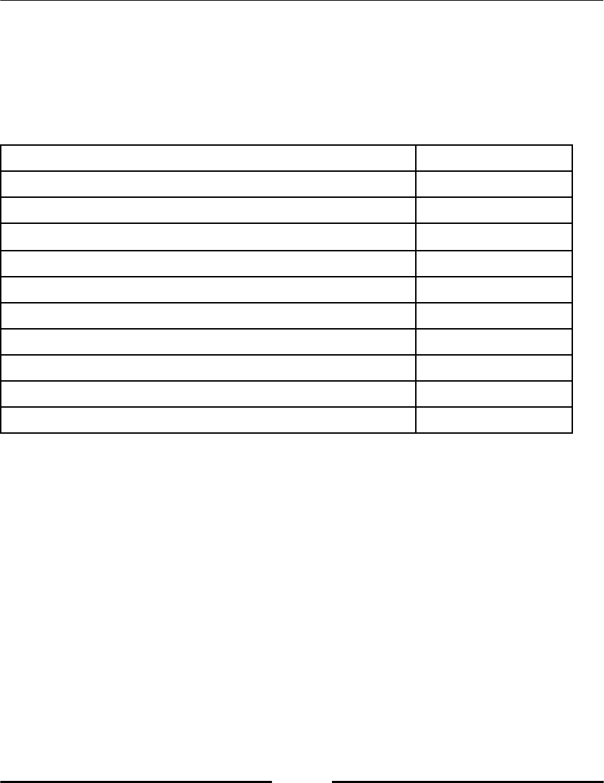
Testing
[ 247 ]
Assertion tools
In this section, we collect the most important tools for raising an AssertionError. We
saw the assert command and two tools from unittest, namely
assertAlmostEqual. The following table (Table 13.1) summarizes the most important
assertion tools and the related modules:
Assertion tool and application example Module
assert 5==5 –
assertEqual(5.27, 5.27) unittest.TestCase
assertAlmostEqual(5.24, 5.2,places = 1) unittest.TestCase
assertTrue(5 > 2) unittest.TestCase
assertFalse(2 < 5) unittest.TestCase
assertRaises(ZeroDivisionError,lambda x: 1/x,0.) unittest.TestCase
assertIn(3,{3,4}) unittest.TestCase
assert_array_equal(A,B) numpy.testing
assert_array_almost_equal(A, B, decimal=5) numpy.testing
assert_allclose(A, B, rtol=1.e-3,atol=1.e-5) numpy.testing
Table 13.1: Assertion tools in Python, unittest and NumPy
Float comparisons
Two floating point numbers should not be compared with the == comparison, because the
result of a computation is often slightly off due to rounding errors. There are numerous
tools to test equality of floats for testing purposes. First, allclose checks that two arrays
are almost equal. It can be used in a test function, as shown:
self.assertTrue(allclose(computed, expected))
Here, self refers to a unittest.Testcase instance. There are also testing tools in the
numpy package testing. These are imported by using:
import numpy.testing

Testing
[ 248 ]
Testing that two scalars or two arrays are equal is done using
numpy.testing.assert_array_allmost_equal or
numpy.testing.assert_allclose. These methods differ in the way they describe the
required accuracy, as shown in the preceding table.
QR factorization decomposes a given matrix into a product of an orthogonal matrix Q and
an upper triangular matrix R as given in the following example:
import scipy.linalg as sl
A=rand(10,10)
[Q,R]=sl.qr(A)
Is the method applied correctly? We can check this by verifying that Q is indeed an
orthogonal matrix:
import numpy.testing as npt
npt.assert_allclose(
dot(Q.T,self.Q),identity(Q.shape[0]),atol=1.e-12)
Furthermore, we might perform a sanity test by checking if A = QR:
import numpy.testing as npt
npt.assert_allclose(dot(Q,R),A))
All this can be collected into a unittest test case as follows:
import unittest
import numpy.testing as npt
from scipy.linalg import qr
from scipy import *
class TestQR(unittest.TestCase):
def setUp(self):
self.A=rand(10,10)
[self.Q,self.R]=qr(self.A)
def test_orthogonal(self):
npt.assert_allclose(
dot(self.Q.T,self.Q),identity(self.Q.shape[0]),
atol=1.e-12)
def test_sanity(self):
npt.assert_allclose(dot(self.Q,self.R),self.A)
if __name__=='__main__':
unittest.main()

Testing
[ 249 ]
Note in assert_allclose the parameter atol defaults to zero, which often causes
problems, when working with matrices having small elements.
Unit and functional tests
Up to now, we have only used functional tests. A functional test checks whether the
functionality is correct. For the bisection algorithm, this algorithm actually finds a zero
when there is one. In that simple example, it is not really clear what a unit test is. Although,
it might seem slightly contrived, it is still possible to make a unit test for the bisection
algorithm. It will demonstrate how unit testing often leads to more compartmentalized
implementation.
So, in the bisection method, we would like to check, for instance, that at each step the
interval is chosen correctly. How to do that? Note that it is absolutely impossible with the
current implementation, because the algorithm is hidden inside the function. One possible
remedy is to run only one step of the bisection algorithm. Since all the steps are similar, we
might argue that we have tested all the possible steps. We also need to be able to inspect the
current bounds a and b at the current step of the algorithm. So we have to add the number
of steps to be run as a parameter and change the return interface of the function. We will do
that as shown:
def bisect(f,a,b,n=100):
...
for iteration in range(n):
...
return a,b
Note that we have to change the existing unit tests in order to accommodate for that change.
We may now add a unit test as shown:
def test_midpoint(self):
a,b = bisect(identity,-2.,1.,1)
self.assertAlmostEqual(a,-0.5)
self.assertAlmostEqual(b,1.)

Testing
[ 250 ]
Debugging
Debugging is sometimes necessary while testing, in particular if it is not immediately clear
why a given test does not pass. In that case, it is useful to be able to debug a given test in an
interactive session. This is however, made difficult by the design of the
unittest.TestCase class, which prevents easy instantiation of test case objects. The
solution is to create a special instance for debugging purpose only.
Suppose that, in the example of the TestIdentity class above, we want to test the
test_functionality method. This would be achieved as follows:
test_case = TestIdentity(methodName='test_functionality')
Now this test can be run individually by:
test_case.debug()
This will run this individual test and it allows for debugging.
Test discovery
If you write a Python package, various tests might be spread out through the package. The
discover module finds, imports, and runs these test cases. The basic call from the
command line is:
python -m unittest discover
It starts looking for test cases in the current directory and recurses the directory tree
downward to find Python objects with the 'test' string contained in its name. The
command takes optional arguments. Most important are -s to modify the start directory
and -p to define the pattern to recognize the tests:
python -m unittest discover -s '.' -p 'Test*.py'
Measuring execution time
In order to take decisions on code optimization, one often has to compare several code
alternatives and decide which code should be preferred based on the execution time.
Furthermore, discussing execution time is an issue when comparing different algorithms. In
this section, we present a simple and easy way to measure execution time.

Testing
[ 251 ]
Timing with a magic function
The easiest way to measure the execution time of a single statement is to use IPython’s
magic function %timeit.
The shell IPython adds additional functionality to standard Python. These
extra functions are called magic functions.
As the execution time of a single statement can be extremely short, the statement is placed
in a loop and executed several times. By taking the minimum measured time, one makes
sure that other tasks running on the computer do not influence the measured result too
much. Let's consider four alternative ways to extract nonzero elements from an array as
follows:
A=zeros((1000,1000))
A[53,67]=10
def find_elements_1(A):
b = []
n, m = A.shape
for i in range(n):
for j in range(m):
if abs(A[i, j]) > 1.e-10:
b.append(A[i, j])
return b
def find_elements_2(A):
return [a for a in A.reshape((-1, )) if abs(a) > 1.e-10]
def find_elements_3(A):
return [a for a in A.flatten() if abs(a) > 1.e-10]
def find_elements_4(A):
return A[where(0.0 != A)]
Measuring time with IPython’s magic function %timeit gives the following result:
In [50]: %timeit -n 50 -r 3 find_elements_1(A)
50 loops, best of 3: 585 ms per loop
In [51]: %timeit -n 50 -r 3 find_elements_2(A)
50 loops, best of 3: 514 ms per loop
In [52]: %timeit -n 50 -r 3 find_elements_3(A)

Testing
[ 252 ]
50 loops, best of 3: 519 ms per loop
In [53]: %timeit -n 50 -r 3 find_elements_4(A)
50 loops, best of 3: 7.29 ms per loop
The parameter -n controls how often the statement is executed before time is measured and
the -r parameter controls the number of repetitions.
Timing with the Python module timeit
Python provides a timeit module, which can be used to measure execution time. It
requires that first a time object is constructed. It is constructed from two strings, a string
with setup commands and a string with the commands to be executed. We take the same
four alternatives as in the preceding example. The array and function definitions are written
now in a string called setup_statements and four-time objects are constructed as follows:
import timeit
setup_statements="""
from scipy import zeros
from numpy import where
A=zeros((1000,1000))
A[57,63]=10.
def find_elements_1(A):
b = []
n, m = A.shape
for i in range(n):
for j in range(m):
if abs(A[i, j]) > 1.e-10:
b.append(A[i, j])
return b
def find_elements_2(A):
return [a for a in A.reshape((-1,)) if abs(a) > 1.e-10]
def find_elements_3(A):
return [a for a in A.flatten() if abs(a) > 1.e-10]
def find_elements_4(A):
return A[where( 0.0 != A)]
"""
experiment_1 = timeit.Timer(stmt = 'find_elements_1(A)',
setup = setup_statements)
experiment_2 = timeit.Timer(stmt = 'find_elements_2(A)',
setup = setup_statements)

Testing
[ 253 ]
experiment_3 = timeit.Timer(stmt = 'find_elements_3(A)',
setup = setup_statements)
experiment_4 = timeit.Timer(stmt = 'find_elements_4(A)',
setup = setup_statements)
The timer objects have a repeat method . It takes repeat and number parameters. It
executes the statement of the timer object in a loop, measures the time, and repeats this
experiment corresponding to the repeat parameter:
We continue the preceding example and measure execution times as shown:
t1 = experiment_1.repeat(3,5)
t2 = experiment_2.repeat(3,5)
t3 = experiment_3.repeat(3,5)
t4 = experiment_4.repeat(3,5)
# Results per loop in ms
min(t1)*1000/5 # 615 ms
min(t2)*1000/5 # 543 ms
min(t3)*1000/5 # 546 ms
min(t4)*1000/5 # 7.26 ms
In contrast to the method in the preceding example, we obtain lists of all the obtained
measurements. As computing time may vary depending on the overall load of the
computer, the minimal value in such a list can be considered a good approximation to the
computation time necessary to execute the statement.
Timing with a context manager
Finally, we present the third method. It serves to show another application of a context
manager. We first construct a context manager object for measuring the elapsed time as
shown:
import time
class Timer:
def __enter__(self):
self.start = time.time()
# return self
def __exit__(self, ty, val, tb):
end = time.time()
self.elapsed=end-self.start
print('Time elapsed {} seconds'.format(self.elapsed))
return False

Testing
[ 254 ]
Recall that the _ _enter_ _ and _ _exit_ _ methods make this class a context manager.
The _ _exit_ _ method’s parameters ty, val, and tb are in the normal case None. If an
exception is raised during execution, they take the exception type, its value, and traceback
information. The return False indicates that the exception has not been caught so far.
We now show the use of the context manager to measure the execution time of the four
alternatives in the previous example:
with Timer():
find_elements_1(A)
This will then display a message like Time elapsed 15.0129795074 ms.
If the timing result should be accessible in a variable, the enter method must return the
Timer instance (uncomment the return statement) and a with ... as ... construction
has to be used:
with Timer() as t1:
find_elements_1(A)
t1.elapsed # contains the result
Summary
No program development without testing! We showed the importance of well organized
and documented tests. Some professionals even start development by first specifying tests.
A useful tool for automatic testing is the module unittest, which we explained in detail.
While testing improves the reliability of a code, profiling is needed to improve the
performance. Alternative ways to code may result in large performance differences. We
showed how to measure computation time and how to localize bottlenecks in your code.
Exercises
Ex. 1 → Two matrices A, B are called similar, if there exists a matrix S, such that B = S-1 A S. A
and B have the same eigenvalues. Write a test checking that two matrices are similar, by
comparing their eigenvalues. Is it a functional or a unit test?
Testing
[ 255 ]
Ex. 2 → Create two vectors of large dimension. Compare the execution time of various ways
to compute their dot product:
SciPy function: dot(v,w)
Generator and sum: sum((x*y for x,y in zip(v,w)))
Comprehensive list and sum: sum([x*y for x,y in zip(v,w)])
Ex. 3 → Let u be a vector. The vector v with components
is called a moving average of u. Determine which of the two alternatives to compute v is
faster:
v = (u[:-2] + u[1:-1] + u[2:]) / 3
or
v = array([(u[i] + u[i + 1] + u[i + 2]) / 3
for i in range(len(u)-3)])

14
Comprehensive Examples
In this chapter, we present some comprehensive and longer examples together with a brief
introduction to the theoretical background and their complete implementation. By this, we
want to show you how the concepts defined in this book are used in practice.
Polynomials
First, we will demonstrate the power of the Python constructs presented so far by designing
a class for polynomials. We will give some theoretical background, which leads us to a list
of requirements, and then we will give the code, with some comments.
Note, this class differs conceptually from the class numpy.poly1d.
Theoretical background
A polynomial: p(x) = an x n + an-1 xn-1+…+ a1x + a0 is defined by its degree, its representation,
and its coefficients. The polynomial representation shown in the preceding equation is
called a monomial representation. In this representation, the polynomial is written as a
linear combination of monomials, xi. Alternatively, the polynomial can be written in:
Newton representation with the coefficients ci and n points, x0, …, xn-1:
p(x) = c0 + c1 (x – x0) + c2 (x – x0)(x-x1) + … + cn(x – x0) … (x – xn-1)
Comprehensive Examples
[ 257 ]
Lagrange representation with the coefficients yi and n+1 points, x0, … , xn:
p(x) = y0 l0(x) + y1 l1(x) + … + yn ln(x)
with the cardinal functions:
There are infinitely many representations, but we restrict ourselves here to these three
typical ones.
A polynomial can be determined from interpolation conditions:
p(xi) = yi i = 0, … , n
with the given distinct values xi and arbitrary values yi as input. In the Lagrange
formulation, the interpolation polynomial is directly available, as its coefficients are the
interpolation data. The coefficients for the interpolation polynomial in Newton
representation can be obtained by a recursion formula, called the divided differences
formula:
ci,0 = yi, and
.
Finally, one sets .
The coefficients of the interpolation polynomial in monomial representation are obtained by
solving a linear system:
Comprehensive Examples
[ 258 ]
A matrix that has a given polynomial p (or a multiple of it) as its characteristic polynomial is
called a companion matrix. The eigenvalues of the companion matrix are the zeros (roots) of
the polynomial. An algorithm for computing the zeros of p can be constructed by first
setting up its companion matrix and then computing the eigenvalues with eig. The
companion matrix for a polynomial in Newton representation reads as follows:
Tasks
We can now formulate some programming tasks:
Write a class called PolyNomial with the points, degree, coeff, and basis1.
attributes, where:
points is a list of tuples (xi, yi)
degree is the degree of the corresponding interpolation polynomial
coeff contains the polynomial coefficients
basis is a string stating which representation is used
Provide the class with a method for evaluating the polynomial at a given point.2.
Provide the class with a method called plot that plots the polynomial over a3.
given interval.
Write a method called __add__ that returns a polynomial that is the sum of two4.
polynomials. Be aware that only in the monomial case the sum can be computed
by just summing up the coefficients.
Write a method that computes the coefficients of the polynomial represented in a5.
monomial form.
Write a method that computes the polynomial's companion matrix.6.

Comprehensive Examples
[ 259 ]
Write a method that computes the zeros of the polynomial by computing the7.
eigenvalues of the companion matrix.
Write a method that computes the polynomial that is the ith derivative of the8.
given polynomial.
Write a method that checks whether two polynomials are equal. Equality can be9.
checked by comparing all coefficients (zero leading coefficients should not
matter).
The polynomial class
Let's now design a polynomial base class based on a monomial formulation of the
polynomial. The polynomial can be initialized either by giving its coefficients with respect
to the monomial basis or by giving a list of interpolation points, as follows:
import scipy.linalg as sl
class PolyNomial:
base='monomial'
def __init__(self,**args):
if 'points' in args:
self.points = array(args['points'])
self.xi = self.points[:,0]
self.coeff = self.point_2_coeff()
self.degree = len(self.coeff)-1
elif 'coeff' in args:
self.coeff = array(args['coeff'])
self.degree = len(self.coeff)-1
self.points = self.coeff_2_point()
else:
self.points = array([[0,0]])
self.xi = array([1.])
self.coeff = self.point_2_coeff()
self.degree = 0
The __init__ method of the new class uses the **args construction as discussed in
section Parameters and arguments in Chapter 7, Functions. If no arguments are given, a zero
polynomial is assumed. If the polynomial is given by interpolation points the method used
to compute the coefficients by solving a Vandermonde system is given as follows:
def point_2_coeff(self):
return sl.solve(vander(self.x),self.y)

Comprehensive Examples
[ 260 ]
If k coefficients are given also k interpolation points are constructed by:
def coeff_2_point(self):
points = [[x,self(x)] for x in linspace(0,1,self.degree+1)]
return array(points)
The self(x) command does a polynomial evaluation, which is done by providing a
method, __call__:
def __call__(self,x):
return polyval(self.coeff,x)
(Refer example in section Special methods in Chapter 8, Classes.) Here, this method uses the
command polyval. As a next step, we just add for convenience two methods, which we
decorate with the property decorator (refer section Functions as decorators in Chapter 7,
Functions):
@property
def x(self):
return self.points[:,0]
@property
def y(self):
return self.points[:,1]
Let's explain what is going on here. We define a method to extract the x-values of the data,
which were used to define the polynomial. Similarly, a method to extract the y-values of the
data is defined. With the property decorator, the result of calling the method is presented
as if it were just an attribute of the polynomial. There are two coding alternatives:
We use a method call:1.
def x(self):
return self.interppoints[:,0]
This gives access to the x-values by the call: p.x().
We use the property decorator. It us to access the x-values simply by this2.
statement: p.x

Comprehensive Examples
[ 261 ]
We choose the second variant. It is always a good practice to define a __repr__ method
(refer section Attributes in Chapter 8, Classes). At least for a quick check of the results, this
method is useful:
def __repr__(self):
txt = 'Polynomial of degree {degree} \n'
txt += 'with coefficients {coeff} \n in {base} basis.'
return txt.format(coeff=self.coeff, degree=self.degree,
base=self.base)
We now provide a method for plotting the polynomial, as follows:
margin = .05
plotres = 500
def plot(self,ab=None,plotinterp=True):
if ab is None: # guess a and b
x = self.x
a, b = x.min(), x.max()
h = b-a
a -= self.margin*h
b += self.margin*h
else:
a,b = ab
x = linspace(a,b,self.plotres)
y = vectorize(self.__call__)(x)
plot(x,y)
xlabel('$x$')
ylabel('$p(x)$')
if plotinterp:
plot(self.x, self.y, 'ro')
Note the use of the vectorize command (refer section Functions acting on arrays in Chapter
4, Linear algebra – Arrays. The __call__ method is specific to the monomial representation
and has to be changed if a polynomial is represented in another basis. This is also the case
for the computation of the polynomial's companion matrix:
def companion(self):
companion = eye(self.degree, k=-1)
companion[0,:] -= self.coeff[1:]/self.coeff[0]
return companion
Once the companion matrix is available, the zeros of the polynomial are given by the
eigenvalues:
def zeros(self):
companion = self.companion()
return sl.eigvals(companion)
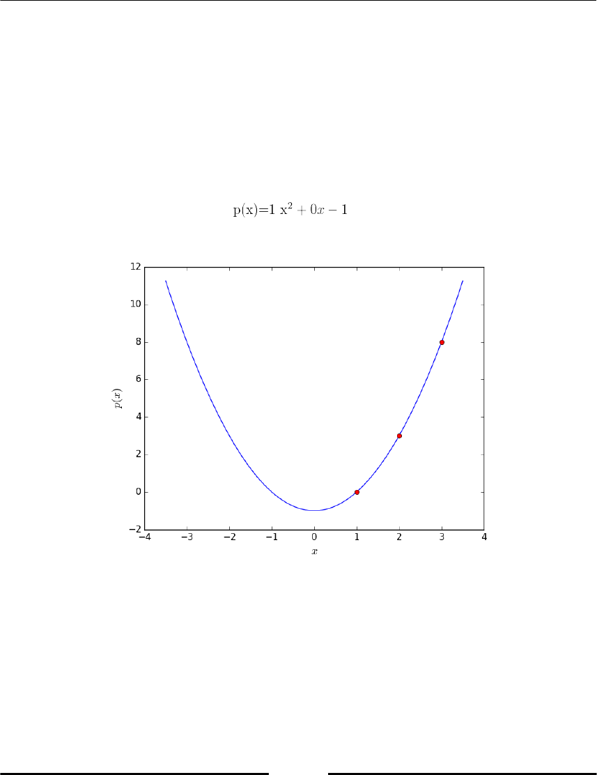
Comprehensive Examples
[ 262 ]
For this end the function eigvals has to be imported from scipy.linalg first. Let's give
some usage examples.
First, we create a polynomial instance from the given interpolation points:
p = PolyNomial(points=[(1,0),(2,3),(3,8)])
The polynomial's coefficients with respect to the monomial basis are available as an
attribute of p:
p.coeff # returns array([ 1., 0., -1.])
This corresponds to the polynomial . The default plot of the polynomial,
obtained by p.plot(-3.5,3.5), results in the following figure (Figure 14.1):
Figure 14.1: Result of the polynomial plot method

Comprehensive Examples
[ 263 ]
Finally, we compute the zeros of the polynomial, which in this case are two real numbers:
pz = p.zeros() # returns array([-1.+0.j, 1.+0.j])
The result can be verified by evaluating the polynomial at these points:
p(pz) # returns array([0.+0.j, 0.+0.j])
Newton polynomial
The NewtonPolyNomial class defines a polynomial described with respect to the Newton
basis. We let it inherit some common methods from the polynomial base class, for example,
polynomial.plot, polynomial.zeros, and even parts of the __init__ method, by
using the super command (refer to section Subclassing and Inheritance in Chapter 8, Classes):
class NewtonPolynomial(PolyNomial):
base = 'Newton'
def __init__(self,**args):
if 'coeff' in args:
try:
self.xi = array(args['xi'])
except KeyError:
raise ValueError('Coefficients need to be given'
'together with abscissae values xi')
super(NewtonPolynomial, self).__init__(**args)
Once the interpolation points are given, the computation of the coefficients is performed by:
def point_2_coeff(self):
return array(list(self.divdiff()))
Here we used divided differences for computing the Newton representation of the
polynomial, which is programmed as a generator here:
def divdiff(self):
xi = self.xi
row = self.y
yield row[0]
for level in range(1,len(xi)):
row = (row[1:] - row[:-1])/(xi[level:] - xi[:-level])
if allclose(row,0): # check: elements of row nearly zero
self.degree = level-1
break
yield row[0]

Comprehensive Examples
[ 264 ]
Let us briefly check how this works:
pts = array([[0.,0],[.5,1],[1.,0],[2,0.]]) # here we define the
interpolation data: (x,y) pairs
pN = NewtonPolynomial(points=pts) # this creates an instance of the
polynomial class
pN.coeff # returns the coefficients array([ 0. , 2. , -4. ,
2.66666667])
print(pN)
The print function executes the __repr__ method of the base class and returns the
following text:
Polynomial of degree 3
with coefficients [ 0. 2. -4. 2.66666667]
in Newton basis.
The polynomial evaluation is different from the corresponding method of the base class.
The Newton.PolyNomial.__call__ method needs to override Polynomial.__call__:
def __call__(self,x):
# first compute the sequence 1, (x-x_1), (x-x_1)(x-x_2),...
nps = hstack([1., cumprod(x-self.xi[:self.degree])])
return dot(self.coeff, nps)
Finally, we give the code for the companion matrix, which overrides the corresponding
method of the parent class, as follows:
def companion(self):
degree = self.degree
companion = eye(degree, k=-1)
diagonal = identity(degree,dtype=bool)
companion[diagonal] = self.x[:degree]
companion[:,-1] -= self.coeff[:degree]/self.coeff[degree]
return companion
Note the use of Boolean arrays. The exercises will further build on this foundation.

Comprehensive Examples
[ 265 ]
Spectral clustering
An interesting application of eigenvectors is for clustering data. Using the eigenvectors of a
matrix derived from a distance matrix, unlabelled data can be separated into groups.
Spectral clustering methods get their name from the use of the spectrum of this matrix. A
distance matrix for n elements (for example, the pairwise distance between data points) is
an n × n symmetric matrix. Given such an n × n distance matrix M with distance values mij,
we can create the Laplacian matrix of the data points as follows:
Here, I is the identity matrix and D is the diagonal matrix containing the row sums of M,
The data clusters are obtained from the eigenvectors of L. In the simplest case of data points
with only two classes, the first eigenvector (that is, the one corresponding to the largest
eigenvalue) is often enough to separate the data.
Here is an example for simple two-class clustering. The following code creates some 2D
data points and clusters them based on the first eigenvector of the Laplacian matrix:
import scipy.linalg as sl
# create some data points
n = 100
x1 = 1.2 * random.randn(n, 2)
x2 = 0.8 * random.randn(n, 2) + tile([7, 0],(n, 1))
x = vstack((x1, x2))
# pairwise distance matrix
M = array([[ sqrt(sum((x[i] - x[j])**2))
for i in range(2*n)]
for j in range(2 * n)])
# create the Laplacian matrix
D = diag(1 / sqrt( M.sum(axis = 0) ))
L = identity(2 * n) - dot(D, dot(M, D))
# compute eigenvectors of L
S, V = sl.eig(L)
# As L is symmetric the imaginary parts
# in the eigenvalues are only due to negligible numerical errors S=S.real
V=V.real
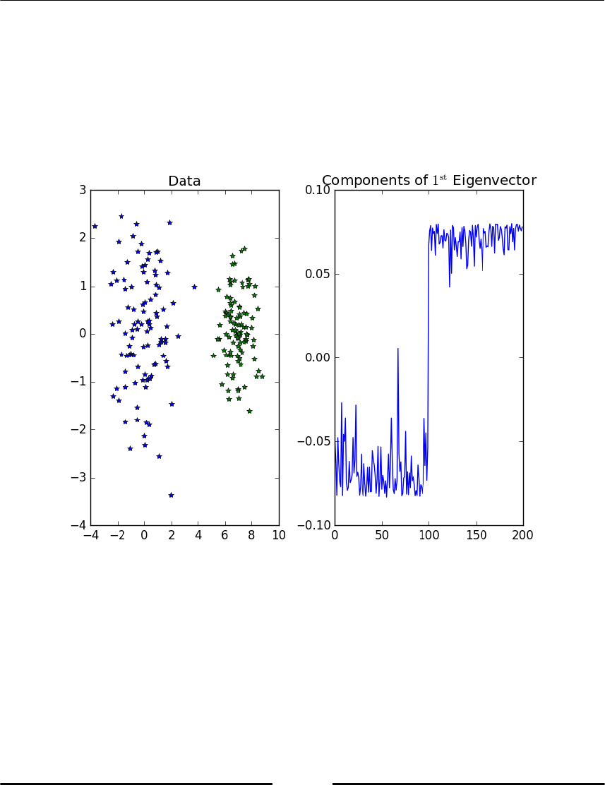
Comprehensive Examples
[ 266 ]
The eigenvector corresponding to the largest eigenvalue gives the grouping (for example,
by thresholding at 0) and can be shown with:
largest=abs(S).argmax()
plot(V[:,largest])
The following figure (Figure 14.2) shows the result of spectral clustering of a simple two-
class dataset:
Figure 14.2: shows result of simple two-class clustering
For more difficult datasets and more classes, one usually takes the k eigenvectors
corresponding to the k largest eigenvalues and then clusters the data with some other
method, but using the eigenvectors instead of the original data points. A common choice is
the k-means clustering algorithm, which is the topic of the next example:

Comprehensive Examples
[ 267 ]
The eigenvectors are used as input to k-means clustering, as follows:
import scipy.linalg as sl
import scipy.cluster.vq as sc
# simple 4 class data
x = random.rand(1000,2)
ndx = ((x[:,0] < 0.4) | (x[:,0] > 0.6)) &
((x[:,1] < 0.4) | (x[:,1] > 0.6))
x = x[ndx]
n = x.shape[0]
# pairwise distance matrix
M = array([[ sqrt(sum((x[i]-x[j])**2)) for i in range(n) ]
for j in range(n)])
# create the Laplacian matrix
D = diag(1 / sqrt( M.sum(axis=0) ))
L = identity(n) - dot(D, dot(M, D))
# compute eigenvectors of L
_,_,V = sl.svd(L)
k = 4
# take k first eigenvectors
eigv = V[:k,:].T
# k-means
centroids,dist = sc.kmeans(eigv,k)
clust_id = sc.vq(eigv,centroids)[0]
Note that we computed the eigenvectors here using the singular value
decomposition, sl.svd. As L is symmetric, the result is the same as if we would have used
sl.eig, but the eigenvectors come already ordered corresponding to the ordering of the
eigenvalues. We also used throw-away variables. svd returns a list with three arrays, the
left and right singular vectors U, V, and the singular values S, as follows:
U, S, V = sl.svd(L)
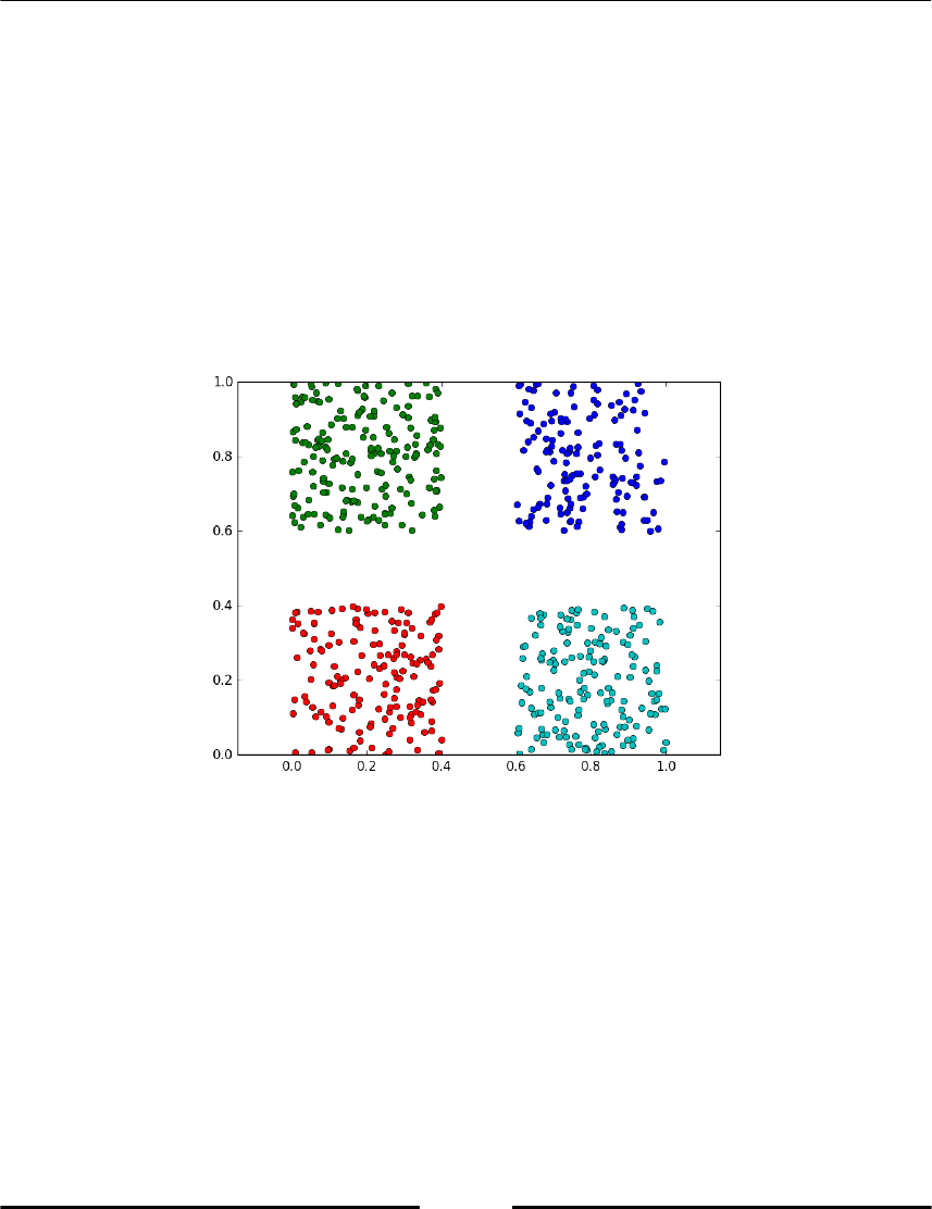
Comprehensive Examples
[ 268 ]
As we do not need U and S here, we can throw them away when unpacking the return
value of svd:
_, _, V = sl.svd(L)
The result can be plotted using:
for i in range(k):
ndx = where(clust_id == i)[0]
plot(x[ndx, 0], x[ndx, 1],'o')
axis('equal')
The following figure shows the result of spectral clustering of a simple multiclass dataset:
Figure 14.3: An example of spectral clustering of a simple four class dataset.
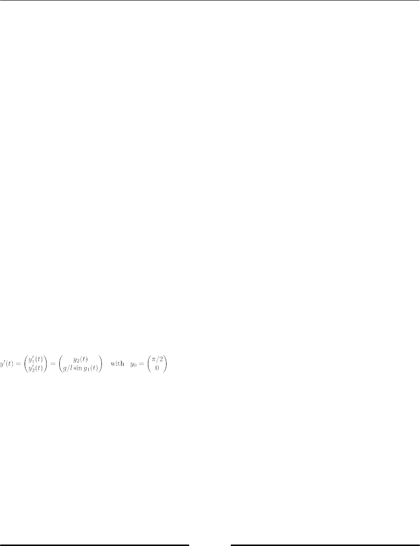
Comprehensive Examples
[ 269 ]
Solving initial value problems
In this section, we will consider the mathematical task of numerically solving a system of
ordinary equations for given initial values:
y'(t) = f(t, y) y(t0) = y0 ∈ ℝn
The solution of this problem is a function y. A numerical method aims at computing good
approximations, yi≈ y(ti) at discrete points, the communications points ti, within the interval
of interest [t0, te]. We collect the data that describes the problem in a class, as follows:
class IV_Problem:
"""
Initial value problem (IVP) class
"""
def __init__(self, rhs, y0, interval, name='IVP'):
"""
rhs 'right hand side' function of the ordinary differential
equation f(t,y)
y0 array with initial values
interval start and end value of the interval of independent
variables often initial and end time
name descriptive name of the problem
"""
self.rhs = rhs
self.y0 = y0
self.t0, self.tend = interval
self.name = name
The differential equation:
describes a mathematical pendulum; y1 describes its angle with respect to the vertical axis, g
is the gravitation constant, and l is its length. The initial angle is π/2 and the initial angular
velocity is zero.

Comprehensive Examples
[ 270 ]
The pendulum problem becomes an instance of the problem class, as follows:
def rhs(t,y):
g = 9.81
l = 1.
yprime = array([y[1], g / l * sin(y[0])])
return yprime
pendulum = IV_Problem(rhs, array([pi / 2, 0.]), [0., 10.] ,
'mathem. pendulum')
There might be different views on the problem at hand, leading to a different design of the
class. For example, one might want to consider the interval of independent variables as a
part of a solution process instead of the problem definition. The same holds when
considering initial values. They might, as we did here, be considered a part of the
mathematical problem, while other authors might want to allow variation of initial values
by putting them as a part of the solution process.
The solution process is modeled as another class:
class IVPsolver:
"""
IVP solver class for explicit one-step discretization methods
with constant step size
"""
def __init__(self, problem, discretization, stepsize):
self.problem = problem
self.discretization = discretization
self.stepsize = stepsize
def one_stepper(self):
yield self.problem.t0, self.problem.y0
ys = self.problem.y0
ts = self.problem.t0
while ts <= self.problem.tend:
ts, ys = self.discretization(self.problem.rhs, ts, ys,
self.stepsize)
yield ts, ys
def solve(self):
return list(self.one_stepper())

Comprehensive Examples
[ 271 ]
We continue by first defining two discretization schemes:
Explicit Euler method:
def expliciteuler(rhs, ts, ys, h):
return ts + h, ys + h * rhs(ts, ys)
Classical Runge-Kutta four-stage method (RK4):
def rungekutta4(rhs, ts, ys, h):
k1 = h * rhs(ts, ys)
k2 = h * rhs(ts + h/2., ys + k1/2.)
k3 = h * rhs(ts + h/2., ys + k2/2.)
k4 = h * rhs(ts + h, ys + k3)
return ts + h, ys + (k1 + 2*k2 + 2*k3 + k4)/6.
With these, we can create instances to obtain the corresponding discretized versions of the
pendulum ODE:
pendulum_Euler = IVPsolver(pendulum, expliciteuler, 0.001)
pendulum_RK4 = IVPsolver(pendulum, rungekutta4, 0.001)
We can solve the two discrete models and plot the solution and the angle difference:
sol_Euler = pendulum_Euler.solve()
sol_RK4 = pendulum_RK4.solve()
tEuler, yEuler = zip(*sol_Euler)
tRK4, yRK4 = zip(*sol_RK4)
subplot(1,2,1), plot(tEuler,yEuler),\
title('Pendulum result with Explicit Euler'),\
xlabel('Time'), ylabel('Angle and angular velocity')
subplot(1,2,2), plot(tRK4,abs(array(yRK4)-array(yEuler))),\
title('Difference between both methods'),\
xlabel('Time'), ylabel('Angle and angular velocity')

Comprehensive Examples
[ 272 ]
Figure14.4: Pendulum simulation with the explicit Euler method and comparison with the
results of the more accurate Runge–Kutta 4 method
It is worthwhile discussing alternative class designs. What should be put in separate classes,
what should be bundled into the same class?
We strictly separated the mathematical problem from the numerical method.
Where should the initial values go? Should they be part of the problem or part of
the solver? Or should they be left as input parameter for the solve method of the
solver instance? One might even design the program so that it allows several
possibilities. The decision to use one of these alternatives depends on the future
use of this program. Looping over various initial values as in parameter
identification would be eased by leaving the initial values as input parameters for
the solve method. On the other hand, simulating different model variants with
the same initial values would motivate to couple the initial values to the problem.
We presented for simplicity only solvers with constant and given step size. Is the
design of the IVPsolver class appropriate for a future extension of adaptive
methods, where a tolerance rather than a step size is given?

Comprehensive Examples
[ 273 ]
We suggested earlier to use a generator construction for the stepping mechanism.
Adaptive methods need to reject steps from time to time. Is this need conflicting
with the design of the stepping mechanism in IVPsolver.onestepper?
We encourage you to check the design of the two SciPy tools for solving initial
values, namely scipy.integrate.ode and scipy.integrate.odeint.
Summary
Most of what we explained in this book is bundled into the three longer examples of this
chapter. They mimic code development and give prototypes, which you are encouraged to
alter and confront with your own ideas.
You saw that code in scientific computing can have its own flavor due to its strong relation
with mathematically defined algorithms and that it is often wise to keep the relationship
between code and formula visible. Python has techniques for this, as you have seen.
Exercises
Ex. 1 → Implement a method __add__, which constructs a new polynomial p+q by adding
two given polynomials p and q. In monomial form, polynomials are added by just adding
the coefficients, whereas in Newton form, the coefficients depend on the abscissa xi of the
interpolation points. Before adding the coefficients of both polynomials, the polynomial q
has to get new interpolation points with the property that their abscissa xi coincides with
those of p and the method __changepoints__ has to be provided for that. It should
change the interpolation points and return a new set of coefficients.
Ex. 2 → Write conversion methods to convert a polynomial from Newton form into
monomial form and vice versa.
Ex. 3 → Write a method called add_point that takes a polynomial q and a tuple (x,y) as
parameters and returns a new polynomial that interpolates self.points and (x,y).
Ex. 4 → Write a class called LagrangePolynomial that implements polynomials in
Lagrange form and inherits as much as possible from the polynomial base class.
Ex. 5 → Write tests for the polynomial class.
15
Symbolic Computations -
SymPy
In this chapter, we will give a brief introduction on using Python for symbolic
computations. There is powerful software in the market for performing symbolic
computations, for example, MapleTM or MathematicaTM. But sometimes, it might be
favorable to make symbolic calculations in the language or framework you are used to. At
this stage of this book, we assume that this language is Python, so we seek for a tool in
Python — the SymPy module.
A complete description of SymPy — if possible, would fill an entire book, and that is not the
purpose of this chapter. Instead, we will stake out a path into this tool by some guiding
examples, giving a flavor of the potential of this tool as a complement to NumPy and SciPy.
What are symbolic computations?
All computations we did so far in this book were so-called numeric computations. These
were a sequence of operations mainly on floating-point numbers. It is the nature of numeric
computations that the result is an approximation of the exact solution.
Symbolic computations operate on formulas or symbols by transforming them as taught in
algebra or calculus into other formulas. The last step of these transformations might then
require that numbers are inserted and a numeric evaluation is performed.
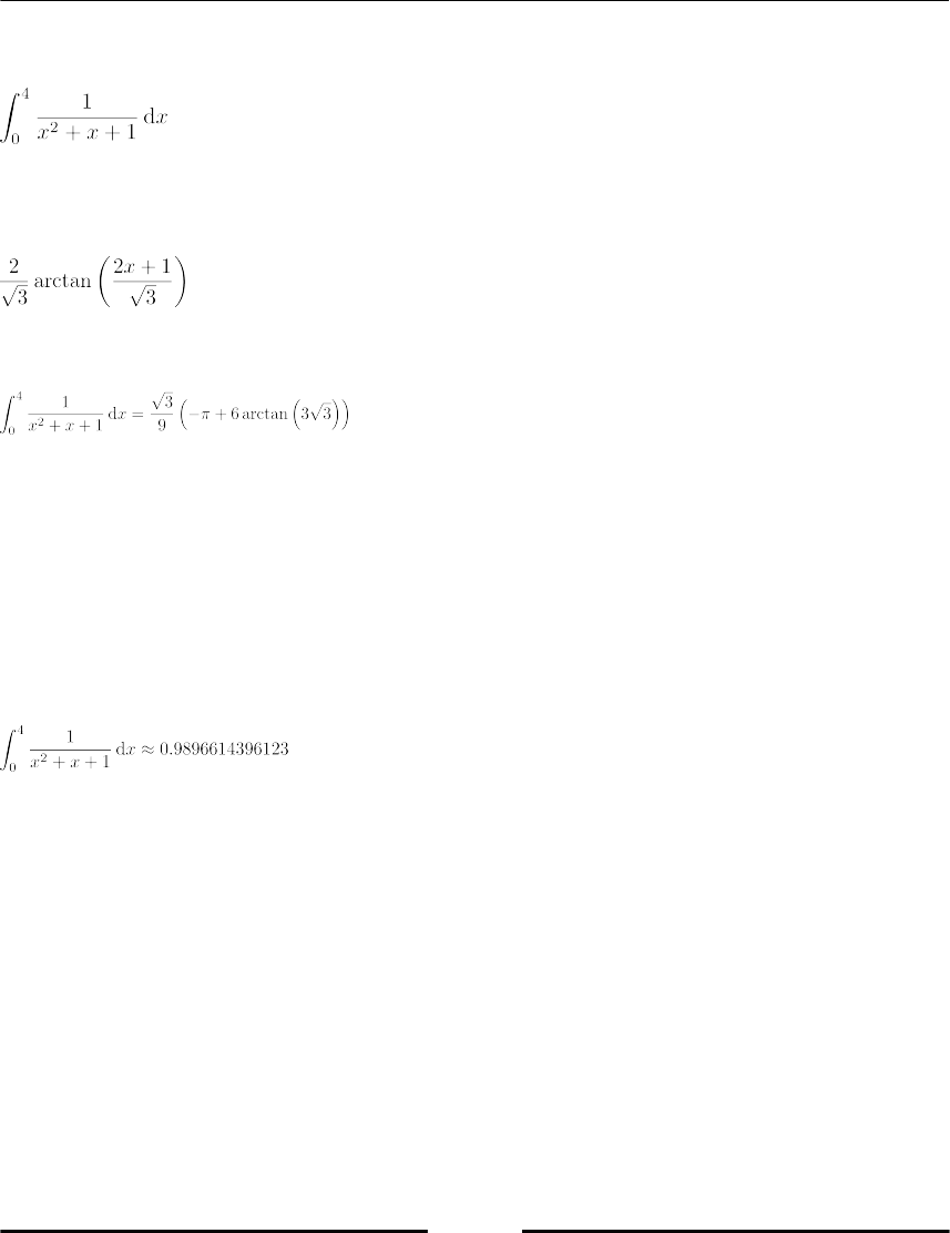
Symbolic Computations - SymPy
[ 275 ]
We illustrate the difference by computing this definite integral:
Symbolically this expression can be transformed by considering the primitive function of
the integrand:
We now obtain a formula for the definite integral by inserting the integral bounds:
This is called a closed-form expression for the integral. Very few mathematical problems
have a solution that can be given in a closed-form expression. It is the exact value of the
integral without any approximation. Also no error is introduced by representing real
numbers as floating-point numbers, which would otherwise introduce round-off errors.
Approximation and round-off come into play at the very last moment, when this expression
needs to be evaluated. The square root and the arctan can only be evaluated approximately
by numerical methods. Such an evaluation gives the final result up to a certain (often
unknown) precision:
On the other hand, numerical computation would directly approximate the definite integral
by some approximation method, for example, Simpson's rule, and deliver a numeric result,
often with an estimate of error. In Python, this is done by these commands:
from scipy.integrate import quad
quad(lambda x : 1/(x**2+x+1),a=0, b=4)
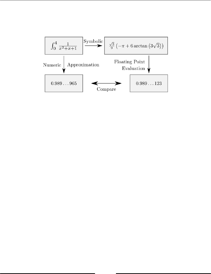
Symbolic Computations - SymPy
[ 276 ]
They return the value 0.9896614396122965 and an estimate for the error bound
1.1735663442283496 10-08.
The following diagram shows the comparison of numeric and symbolic approximation:
Figure 15.1: Symbolic and numeric quadrature
Elaborating an example in SymPy
To begin with, let's elaborate the previous example in SymPy which are explained the steps.
First, we have to import the module:
from sympy import *
init_printing()
The second command makes sure that formulas are presented in a graphical way, if
possible. Then, we generate a symbol and define the integrand:
x = symbols('x')
f = Lambda(x, 1/(x**2 + x + 1))
x is now a Python object of type Symbol and f is a SymPy Lambda function (note the
command starting with a capital letter).
Now we start with the symbolic computation of the integral:
integrate(f(x),x)
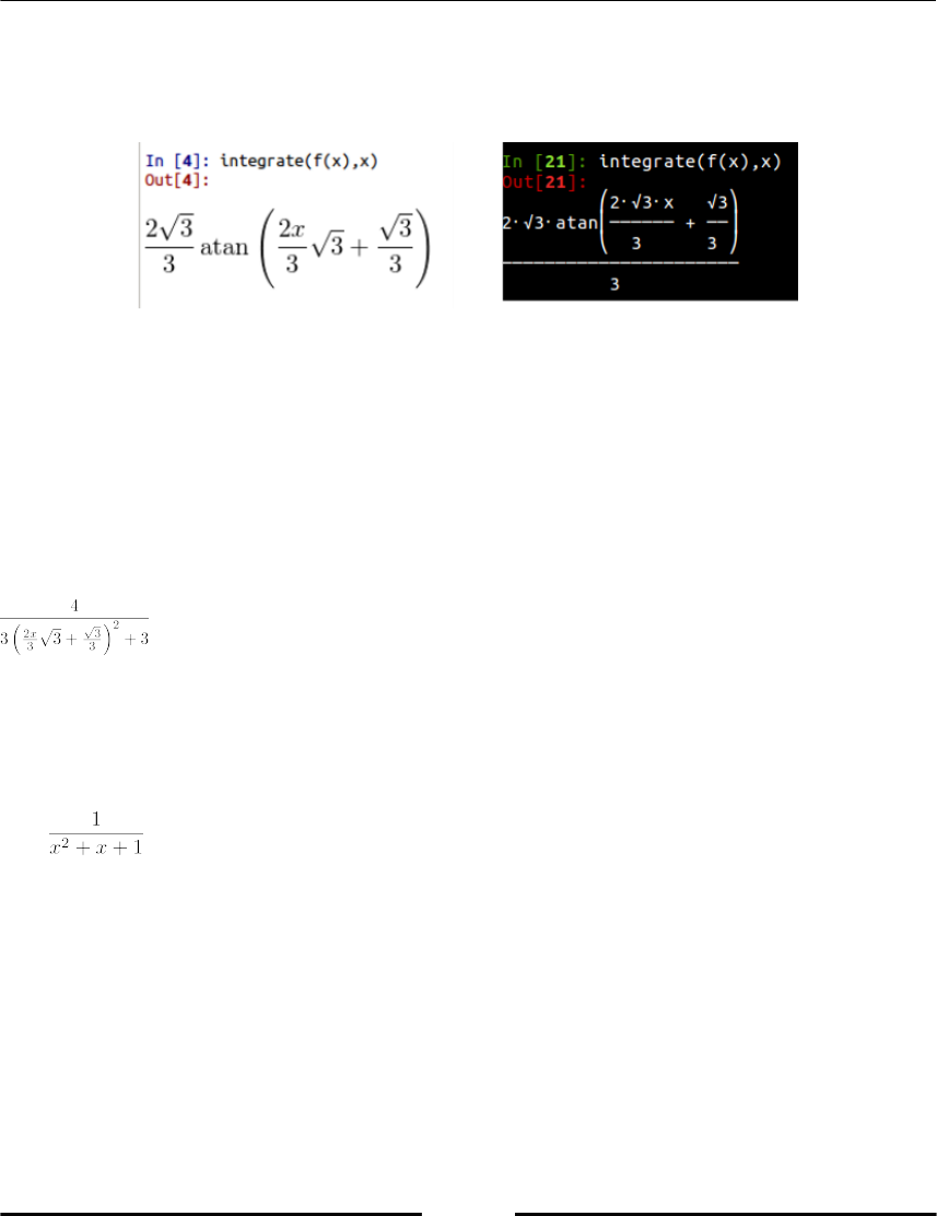
Symbolic Computations - SymPy
[ 277 ]
Depending on your working environment, the result is presented in different ways; refer to
following screenshot (Figure 15.2) which represents two different result of SymPy formula
in different environments:
Figure 15.2: Two screenshots of a SymPy presentation of a formula in two different
environments.
We can check by differentiation whether the result is correct. To this end, we assign a name
to the primitive function and differentiate with respect to x:
pf = Lambda(x, integrate(f(x),x))
diff(pf(x),x)
The result obtained will be as follows:
which can be simplified by using the following command:
simplify(diff(pf(x),x))
to
.
The result we expected.
The definite integral is obtained by using the following command:
pf(4) - pf(0)
Symbolic Computations - SymPy
[ 278 ]
It gives the following output after simplification with simplify:
To obtain a numerical value, we finally evaluate this expression to a floating-point number:
(pf(4)-pf(0)).evalf() # returns 0.9896614396123
Basic elements of SymPy
Here we introduce the basic elements of SymPy. You will find it favorable to be already
familiar with classes and data types in Python.
Symbols – the basis of all formulas
The basic construction element to build a formula in SymPy is the symbol. As we saw in the
introductory example, a symbol is created by the command symbols. This SymPy
command generates symbol objects from a given string:
x, y, mass, torque = symbols('x y mass torque')
It is actually a short form of following command:
symbol_list=[symbols(l) for l in 'x y mass torque'.split()]
followed by a unpacking step to obtain variables:
x, y, mass, torque = symbol_list
The arguments of the command define the string representation of the symbol. The variable
name of the symbol is often chosen identical to its string representation, but this is not
required by the language:
row_index=symbols('i',integer=True)
print(row_index**2) # returns i**2
Here, we also defined that the symbol is assumed to be an integer.

Symbolic Computations - SymPy
[ 279 ]
An entire set of symbols can be defined in a very compact way:
integervariables = symbols('i:l', integer=True)
dimensions = symbols('m:n', integer=True)
realvariables = symbols('x:z', real=True)
Similarly, symbols for indexed variables can be defined by using the following:
A = symbols('A1:3(1:4)')
This gives a tuple of symbols,
The rules for the range of the indexes are those we saw earlier in this book when working
with slices (refer Chapter 3, Container Types for more details).
Numbers
Python evaluates operations on numbers directly and introduces unavoidably rounding
errors. These would obstruct all symbolic calculations. This is avoided when we sympify
numbers:
1/3 # returns 0.3333333333333333
sympify(1)/sympify(3) # returns '1/3'
The sympify command converts an integer to an object of type
sympy.core.numbers.Integer.
Instead of writing 1/3 as an operation of two integers, it can also be represented directly as a
rational number by Rational(1,3).
Functions
SymPy distinguishes between defined and undefined functions. The term undefined
functions (might be a bit misleading) refers to well-defined Python objects for generic
functions that have no special properties.
An example of a function with special properties is atan or the Lambda function used in the
introductory example of this chapter.
Symbolic Computations - SymPy
[ 280 ]
Note the different names for the different implementations of the same mathematical
function: sympy.atan and scipy.arctan.
Undefined functions
A symbol for an undefined function is created by giving the symbols command an extra
class argument:
f, g = symbols('f g', cls=Function)
The same can be achieved by using the Function constructor:
f = Function('f')
g = Function('g')
with undefined functions, we can evaluate general rules of calculus.
For example, let us evaluate the following expression:
This is symbolically computed in Python by using the following command:
x = symbols('x')
f, g = symbols('f g', cls=Function)
diff(f(x*g(x)),x)
When executed, the previous code returns the following as output:
This example shows how the product rule and the chain rule were applied.
We can even use undefined functions as a function in several variables, for example:
x = symbols('x:3')
f(*x)
which returns the following output:
Symbolic Computations - SymPy
[ 281 ]
Note the use of the star operator to unpack a tuple to form f with
arguments; refer to section Anonymous functions, Chapter 7, Functions
By using list comprehension, we can construct a list of all partial derivatives of f :
[diff(f(*x),xx) for xx in x]
This returns a list with the elements of (the gradient of f):
The command can also be rewritten by using the diff method of the Function object:
[f(*x).diff(xx) for xx in x]
Another method is Taylor series expansion :
x = symbols('x')
f(x).series(x,0,n=4)
This returns Taylor's formula, together with the rest term expressed by the Landau symbol:
Elementary Functions
Examples for elementary functions in SymPy are trigonometric functions and their inverses.
The following example shows how simplify acts on expression which include elementary
function:
x = symbols('x')
simplify(cos(x)**2 + sin(x)**2) # returns 1
Here is another example for the use of elementary functions:
atan(x).diff(x) - 1./(x**2+1) # returns 0
Symbolic Computations - SymPy
[ 282 ]
If you use SciPy and SymPy together, we strongly recommend that you use them in
different namespaces:
import scipy as sp
import sympy as sym
# working with numbers
x=3
y=sp.sin(x)
# working with symbols
x=sym.symbols('x')
y=sym.sin(x)
Lambda – functions
In section Anonymous functions of Chapter 7, Functions, we saw how to define so-called
anonymous functions in Python. The counterpart in SymPy is done by the Lambda
command. Note the difference; lambda is a keyword while Lambda is a constructor.
The command Lambda takes two arguments, the symbol of the function's independent
variable, and a SymPy expression to evaluate the function.
Here is an example that defines air resistance (also called drag) as a function of speed:
C,rho,A,v=symbols('C rho A v')
# C drag coefficient, A coss-sectional area, rho density
# v speed
f_drag = Lambda(v,-Rational(1,2)*C*rho*A*v**2)
f_drag is displayed as an expression:
.
This function can be evaluated in the usual way by providing it with an argument:
x = symbols('x')
f_drag(2)
f_drag(x/3)
which will results in given expression:

Symbolic Computations - SymPy
[ 283 ]
It is also possible to create functions in several variables by just providing it with several
arguments as for example:
t=Lambda((x,y),sin(x) + cos(2*y))
A call to this function can be done in two ways, either by directly providing several
arguments:
t(pi,pi/2) # returns -1
or by unpacking a tuple or list:
p=(pi,pi/2)
t(*p) # returns -1
Matrix objects in SymPy make it even possible to define vector-valued functions:
F=Lambda((x,y),Matrix([sin(x) + cos(2*y), sin(x)*cos(y)]))
This enables us to compute Jacobians:
F(x,y).jacobian((x,y))
Which gives the following expression as output:
In the case of more variables, it is convenient to use a more compact form to define the
function:
x=symbols('x:2')
F=Lambda(x,Matrix([sin(x[0]) + cos(2*x[1]),sin(x[0])*cos(x[1])]))
F(*x).jacobian(x)
Symbolic Linear Algebra
Symbolic linear algebra is supported by SymPy's matrix data type which we will introduce
first.
Then we will present some linear algebra methods as examples for the broad spectrum of
possibilities for symbolic computations in this field:
Symbolic Computations - SymPy
[ 284 ]
Symbolic matrices
We briefly met the matrix data type when we discussed vector valued functions. There, we
saw it in its simplest form, which converts a list of lists into a matrix. To have an example,
let's construct a rotation matrix:
phi=symbols('phi')
rotation=Matrix([[cos(phi), -sin(phi)],
[sin(phi), cos(phi)]])
When working with SymPy matrices we have to note that the operator * performs matrix
multiplications and is not acting as an elementwise multiplication which is the case for
NumPy arrays.
The above defined rotation matrix can be checked for orthogonality, by using this matrix
multiplication and the transpose of a matrix:
simplify(rotation.T*rotation -eye(2)) # returns a 2 x 2 zero matrix
The previous example shows how a matrix is transposed and how the identity matrix is
created. Alternatively, we could have checked whether its inverse is its transpose, which
can be done as:
simplify(rotation.T - rotation.inv())
Another way to set up a matrix is by providing a list of symbols and a shape:
M = Matrix(3,3, symbols('M:3(:3)'))
This creates the following matrix:
A third way to create a matrix is by generating its entries by a given function. The syntax is:
Matrix(number of rows,number of colums, function)
We exemplify the above matrix by considering Toeplitz matrix is a matrix with constant
diagonals. Given a 2n-1 data vector a, its elements are defined as
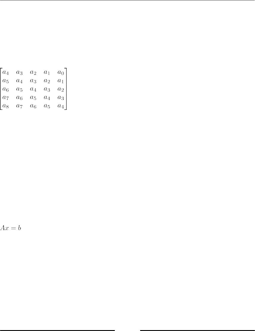
Symbolic Computations - SymPy
[ 285 ]
In SymPy, the matrix can be defined by directly making use of this definition:
def toeplitz(n):
a = symbols('a:'+str(2*n))
f = lambda i,j: a[i-j+n-1]
return Matrix(n,n,f)
Executing the previous code gives toeplitz(5):
One clearly sees the desired structures; all elements along subdiagonals and superdiagonals
are the same. We can access matrix elements by the indexes and slices according to the
Python syntax introduced in the section Lists of Chapter 3, Container Type:
a=symbols('a')
M[0,2]=0 # changes one element
M[1,:]=Matrix(1,3,[1,2,3]) # changes an entire row
Examples for Linear Algebra Methods in
SymPy
The basic task in linear algebra is to solve linear equation systems:
.
Let us do this symbolically for a 3 × 3 matrix:
A = Matrix(3,3,symbols('A1:4(1:4)'))
b = Matrix(3,1,symbols('b1:4'))
x = A.LUsolve(b)
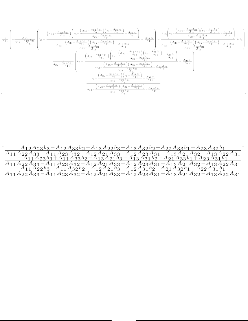
Symbolic Computations - SymPy
[ 286 ]
The output of this relatively small problem is already merely readable which can be seen in
the following expression:
Again, the use of simplify command helps us to detect canceling terms and to collect
common factors:
simplify(x)
which will result in the following output which looks much better:
Symbolic computations becomes very slow with increase in matrix dimensions. For
dimensions bigger than 15, there might even occur memory problems.
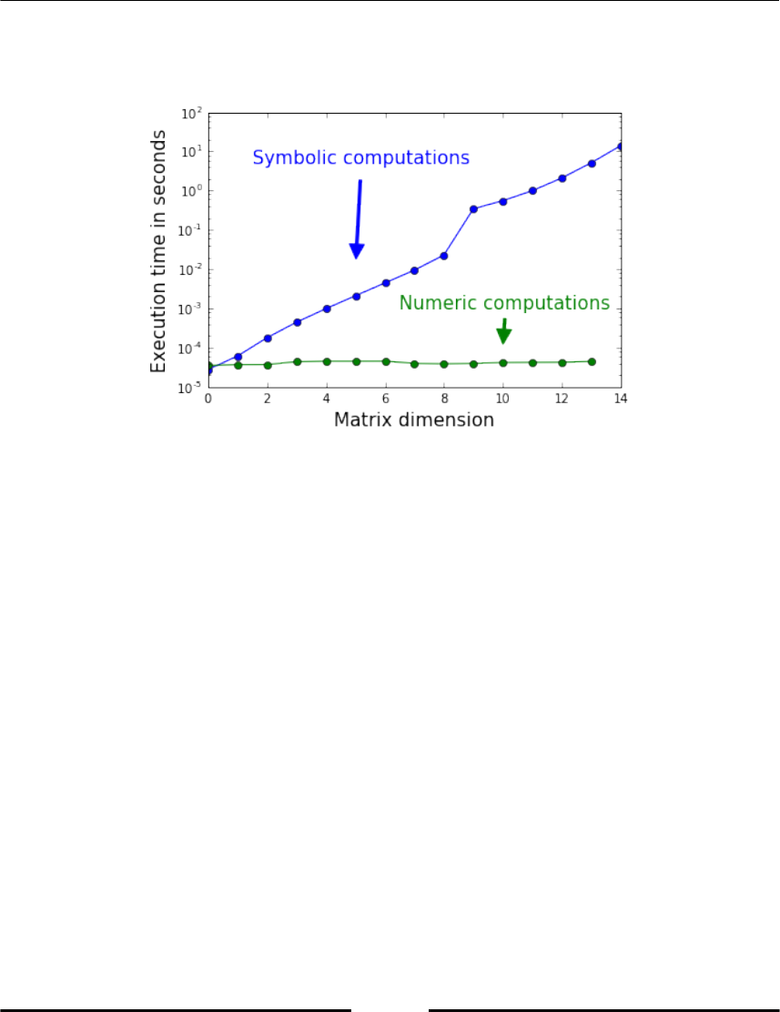
Symbolic Computations - SymPy
[ 287 ]
The preceding figure (Figure 15.3) illustrates the differences in CPU time between
symbolically and numerically solving a linear system:
Figure 15.3: CPU time for numerically and symbolically solving a linear
system.
Substitutions
Let us first consider a simple symbolic expression:
x, a = symbols('x a')
b = x + a
What happens if we set x = 0 ? We observe that b did not change. What we did was that
we changed the Python variable x. It now no longer refers to the symbol object but to the
integer object 0. The symbol represented by the string 'x' remains unaltered, and so does
b.
Instead, altering an expression by replacing symbols by numbers, other symbols, or
expressions is done by a special substitution method which can be seen in following code:
x, a = symbols('x a')
b = x + a
c = b.subs(x,0)
d = c.subs(a,2*a)
print(c, d) # returns (a, 2a)
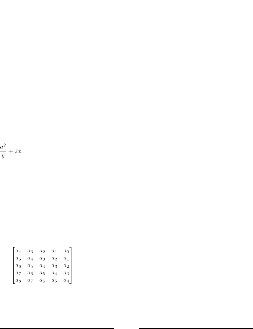
Symbolic Computations - SymPy
[ 288 ]
This method takes one or two arguments:
b.subs(x,0)
b.subs({x:0}) # a dictionary as argument
Dictionaries as arguments allow us to make several substitutions in one step:
b.subs({x:0, a:2*a}) # several substitutions in one
As items in dictionaries have no defined order – one never knows which would be the first
– there is a need for assuring that permuting the items would not affect the substitution
result. Therefore in SymPy, substitutions are first made within the dictionary and then on
the expression. This is demonstrated by the following example:
x, a, y = symbols('x a y')
b = x + a
b.subs({a:a*y, x:2*x, y:a/y})
b.subs({y:a/y, a:a*y, x:2*x})
Both substitutions return the same result, that is,
.
A third alternative to define multiple substitutions is by using a list of old-value/ new-value
pairs instead:
b.subs([(y,a/y), (a,a*y), (x,2*x)])
It is also possible to substitute entire expressions by others:
n, alpha = symbols('n alpha')
b = cos(n*alpha)
b.subs(cos(n*alpha), 2*cos(alpha)*cos((n-1)*alpha)-cos((n-2)*alpha))
To illustrate substitutions of matrix elements, we take the 5 × 5 Toeplitz matrix again:
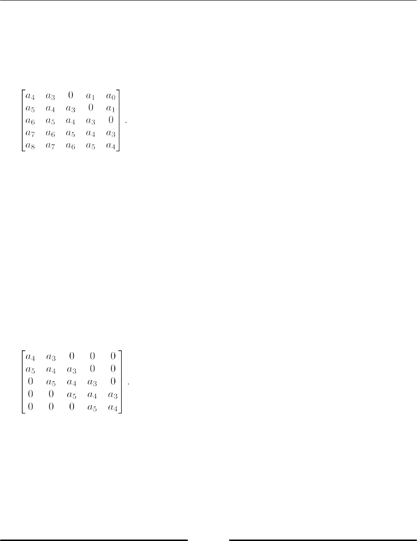
Symbolic Computations - SymPy
[ 289 ]
Consider the substitution M.subs(T[0,2],0). It changes the symbol object at position [0,
2], which is the symbol a2. It also occurs at two other places, which are automatically
affected by this substitution.
The given expression is the resulting matrix:
Alternatively we can create a variable for this symbol and use it in the substitution:
a2 = symbols('a2')
T.subs(a2,0)
As a more complex example for substitution we describe, how to turn the Toeplitz matrix
into a tridiagonal Toeplitz matrix. This can be done in the following ways:
First we generate a list of those symbols that we want to substitute; and then we use the zip
command to generate a list of pairs. Finally we substitute by giving a list of old-value/new-
value pairs as described above:
symbs = [symbols('a'+str(i)) for i in range(19) if i < 3 or i > 5]
substitutions=list(zip(symbs,len(symbs)*[0]))
T.subs(substitutions)
This gives the following matrix as result:
Evaluating symbolic expressions
In the context of scientific computing, there is often the need of first making symbolic
manipulations and then converting the symbolic result into a floating-point number .
Symbolic Computations - SymPy
[ 290 ]
The central tool for evaluating a symbolic expression is evalf. It converts symbolic
expressions to floating-point numbers by using the following:
pi.evalf() # returns 3.14159265358979
The data type of the resulting object is Float (note the capitalization), which is a SymPy
data type that allows floating-point numbers with an arbitrary number of digits (arbitrary
precision).
The default precision corresponds to 15 digits, but it can be changed by giving evalf an
extra positive integer argument specifying the desired precision in terms the numbers of
digits,
pi.evalf(30) # returns 3.14159265358979323846264338328
A consequence of working with arbitrary precision is that numbers can be arbitrary small,
that is, the limits of the classical floating-point representation are broken; refer Floating Point
Numbers section in Chapter 2, Variables and Basic Types.
Interestingly enough, evaluating a SymPy function with an input of type Float returns a
Float with the same precision as the input. We demonstrate the use of this fact in a more
elaborated example from numerical analysis.
Example: A study on the convergence order of
Newton's Method
An iterative method with iterates xn is said to converge with order q with , if there
exists a positive constant C such that
.
Newton's method when started with a good initial has order q = 2, and for certain problems,
even q = 3. Newton's method when applied to the problem arctan(x) = 0 gives the following
iteration scheme:
which converges cubically; that is q = 3.
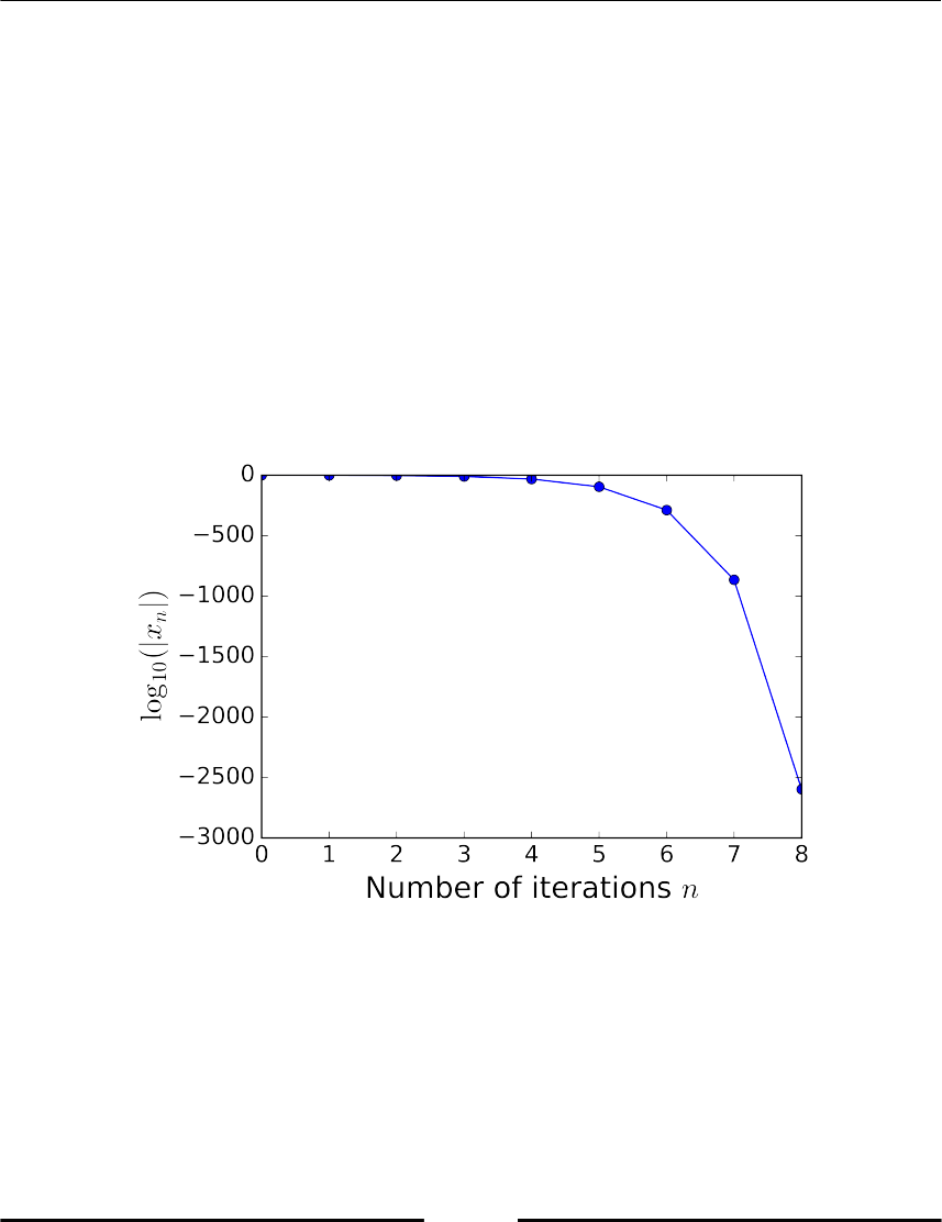
Symbolic Computations - SymPy
[ 291 ]
This implies that the number of correct digits triples from iteration to iteration. To
demonstrate cubic convergence and to numerically determine the constant C is hardly
possible with the standard 16-digit float data type.
The following code, uses SymPy together with high-precision evaluation instead and puts a
study on cubic convergence to the extreme:
x = sp.Rational(1,2)
xns=[x]
for i in range(1,9):
x = (x - sp.atan(x)*(1+x**2)).evalf(3000)
xns.append(x)
The result is depicted in the next figure (Figure 15.4) which shows that the number of correct
digits triples from iteration to iteration.
Figure 15.4: A study on the convergence of Newton's method applied to
arctan(x)=0
This extreme precision requirement (3,000 digits!) enables us to evaluate seven terms of the
preceding sequence to demonstrate cubic convergence in the following way:
# Test for cubic convergence
print(array(abs(diff(xns[1:]))/abs(diff(xns[:-1]))**3,dtype=float64))

Symbolic Computations - SymPy
[ 292 ]
The result is a list of seven terms which let us assume that C = 2/3:
[ 0.41041618, 0.65747717, 0.6666665, 0.66666667, 0.66666667, 0.66666667,
0.66666667]
Converting a symbolic expression into a
numeric function
As we have seen the numerical evaluation of a symbolic expression is done in three steps,
first we do some symbolic computations and then we substitute values by numbers and do
an evaluation to a floating point number by evalf.
The reason for symbolic computations is often that one wants to make parameter studies.
This requires that the parameter is modified within a given parameter range. This requires
that an symbolic expression is eventually turned into a numeric function.
A study on the parameter dependency of
polynomial coefficients
We demonstrate a symbolic/ numeric parameter study by an interpolation example to
introduce the SymPy command lambdify.
Let us consider the task to interpolate the data x = [0, t, 1] and y = [0, 1,-1]. Here, t is a free
parameter, which we will vary over the interval [-0.4, 1.4].
The quadratic interpolation polynomial has coefficients depending on this parameter:
.
Using SymPy and the monomial approach described in gives us closed formulas for these
coefficients:
t=symbols('t')
x=[0,t,1]
# The Vandermonde Matrix
V = Matrix([[0, 0, 1], [t**2, t, 1], [1, 1,1]])
y = Matrix([0,1,-1]) # the data vector
a = simplify(V.LUsolve(y)) # the coefficients
# the leading coefficient as a function of the parameter
a2 = Lambda(t,a[0])
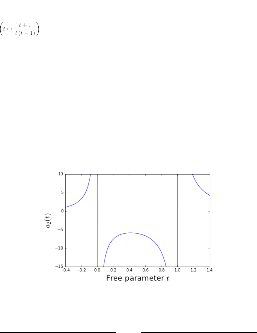
Symbolic Computations - SymPy
[ 293 ]
We obtain a symbolic function for the leading coefficient a2 of the interpolation polynomial:
Now it is time to turn the expression into a numeric function, for example, to make a plot.
This is done by the function lamdify. This function takes two arguments, the independent
variable and a SymPy function.
For our example in Python we can write:
leading_coefficient = lambdify(t,a2(t))
This function can now be plotted, for example, by the following commands:
t_list= linspace(-0.4,1.4,200)
ax=subplot(111)
lc_list = [leading_coefficient(t) for t in t_list]
ax.plot(t_list, lc_list)
ax.axis([-.4,1.4,-15,10])
The preceding figure (Figure 15.5) is the result of this parameter study, one clearly sees the
singularities due to multiple interpolation points, (here at t = 0 or t = 1):
Figure 15.5: The dependency of a polynomial coefficient on the location of an interpolation point.

Symbolic Computations - SymPy
[ 294 ]
Summary
In this chapter you were introduced in the world of symbolic computations and you got a
glimpse of the power of SymPy. By guiding examples you learned how to set up symbolic
expressions, how to work with symbolic matrices, and you saw how to make
simplifications. Working with symbolic functions and transforming them into numerical
evaluations built finally the link to scientific computing and floating point results. You
experienced the strength of SymPy as you used its full integration into Python with its
powerful constructs and legible syntax.
Consider this last chapter as an appetizer rather than a complete menu. We hope you
became hungry for future fascinating programming challenges in scientific computing and
mathematics.
References
M. Abramowitz and I.A. Stegun, Handbook of Mathematical Functions with1.
Formulas, Graphs, and Mathematical Tables, U.S. Department of Commerce, 2002.
ISBN: 9780486612720.
Anaconda – Continuum Analytics Download page. URL: h t t p s ://w w w . c o n t i n u u m . i2.
o /d o w n l o a d s .
Michael J. Cloud, Moore Ramon E., and R. Baker Kearfott, Introduction to Interval3.
Analysis, Society for Industrial and Applied Mathematics (SIAM), 2009. ISBN:
0-89871-669-1.
Python Decorator Library. URL: h t t p ://w i k i . p y t h o n . o r g /m o i n /P y t h o n D e c o r a t o4.
r L i b r a r y .
Z. Bai E. Anderson, C. Bischof, S. Blackford, J. Demmel, J. Dongarra, J. Du Croz,5.
A. Greenbaum, S. Hammarling, A. McKenney, and D. Sorensen, LAPACK Users’
Guide, SIAM, 1999. ISBN: 9780898714470.
fraction – Rational Numbers Library. URL: h t t p ://d o c s . p y t h o n . o r g /l i b r a r y /f r a6.
c t i o n s . h t m l .
Claus Führer, Jan Erik Solem, and Olivier Verdier, Computing with Python,7.
Pearson, 2014. ISBN: 978-0-273-78643-6.
functools – Higher order functions and operations on callable objects. URL: h t t p ://d o c8.
s . p y t h o n . o r g /l i b r a r y /f u n c t o o l s . h t m l .
Python Generator Tricks. URL: h t t p ://l i n u x g a z e t t e . n e t /100/p r a m o d e . h t m l .9.
G.H. Golub and C.F.V. Loan, Matrix computations, Johns Hopkins studies in the10.
mathematical sciences. Johns Hopkins University Press, 1996. ISBN:
9780801854149.
Ernst Hairer and Gerhard Wanner, Analysis by its history, Springer, 1995.11.
Python versus Haskell. URL: h t t p ://w i k i . p y t h o n . o r g /m o i n /P y t h o n V s H a s k e l l .12.

References
[ 296 ]
The IEEE 754-2008 standard. URL: h t t p ://e n . w i k i p e d i a . o r g /w i k i /I E E E _ 754-13.
2008.
Interval arithmetic. URL: h t t p ://e n . w i k i p e d i a . o r g /w i k i /I n t e r v a l _ a r i t h m e t i c14.
.
IPython: Interactive Computing. URL: h t t p ://i p y t h o n . o r g /.15.
H.P. Langtangen, Python scripting for computational science (Texts in computational16.
science and engineering), Springer, 2008. ISBN:9783540739159.
H.P. Langtangen, A Primer on Scientific Programming with Python (Texts in17.
Computational Science and Engineering), Springer, 2009. ISBN: 9783642024740.
D. F. Lawden, Elliptic Functions and Applications, Springer, 1989. ISBN:18.
9781441930903.
M. Lutz, Learning Python: Powerful Object-Oriented Programming, O’Reilly, 2009.19.
ISBN: 9780596158064.
NumPy Tutorial – Mandelbrot Set Example. URL: h t t p ://w w w . s c i p y . o r g /T e n t a t i20.
v e _ N u m P y _ T u t o r i a l /M a n d e l b r o t _ S e t _ E x a m p l e .
matplotlib. URL: h t t p ://m a t p l o t l i b . s o u r c e f o r g e . n e t .21.
Standard: Memoized recursive Fibonacci in Python. URL: h t t p ://u j i h i s a . b l o g s p o t22.
. s e /2010/11/m e m o i z e d - r e c u r s i v e - f i b o n a c c i i n - p y t h o n . h t m l .
Matplotlib mplot3d toolkit. URL: h t t p ://m a t p l o t l i b . s o u r c e f o r g e . n e t /m p l _ t o o l23.
k i t s /m p l o t 3d .
James M. Ortega and Werner C. Rheinboldt, Iterative solution of nonlinear equations24.
in several variables, SIAM, 2000. ISBN: 9780898714616.
pdb – The Python Debugger, documentation: h t t p ://d o c s . p y t h o n . o r g /l i b r a r y /p25.
d b . h t m l .
Fernando Pérez and Brian E. Granger. IPython: a System for Interactive Scientific26.
Computing.” In: Comput. Sci. Eng. 9.3 (May 2007), pp. 21–29. URL: h t t p ://i p y t h
o n . o r g .
Michael J.D. Powell. “An efficient method for finding the minimum of a function27.
of several variables without calculating derivatives.” In: Computer Journal 7 (2
1964), pp. 155–162. doi: doi:10.1093/comjnl/7.2.155.
Timothy Sauer, Numerical Analysis, Pearson, 2006.28.
L.F. Shampine, R.C. Allen, and S. Pruess, Fundamentals of Numerical Computing,29.
John Wiley, 1997. ISBN: 9780471163633.
Jan Erik Solem, Programming Computer Vision with Python, O’Reilly Media, 2012.30.
URL: h t t p ://p r o g r a m m i n g c o m p u t e r v i s i o n . c o m .
Python Documentation – Emulating numeric types. URL: h t t p ://d o c s . p y t h o n . o r g31.
/r e f e r e n c e /d a t a m o d e l . h t m l #e m u l a t i n g - n u m e r i c - t y p e s .

References
[ 297 ]
Sphinx: Python Documentation Generator. URL: h t t p ://s p h i n x . p o c o o . o r g /.32.
J. Stoer and R. Bulirsch, Introduction to numerical analysis. Texts in applied33.
mathematics, Springer, 2002. ISBN: 9780387954523.
Python Format String Syntax. URL: h t t p ://d o c s . p y t h o n . o r g /l i b r a r y /s t r i n g . h34.
t m l #f o r m a t - s t r i n g - s y n t a x .
S. Tosi, Matplotlib for Python Developers, Packt Publishing, 2009. ISBN:35.
9781847197900.
Lloyd N. Trefethen and David Bau, Numerical Linear Algebra, SIAM: Society for36.
Industrial and Applied Mathematics, 1997. ISBN: 0898713617.
visvis – The object oriented approach to visualization. URL: http37.
://code.google.com/p/visvis/.
The full list of built-in exceptions can be found at h t t p ://d o c s . p y t h o n . o r g /38.
library/exceptions.html
Index
%
%matplotlib command 119
3
3D plots
creating 141, 144
A
AGM iteration 196
allclose command 68
Anaconda
about 12
installing 12
annotations
about 137
example 137
anonymous functions
about 161
Lambda construction 162
arguments
about 150
default arguments 153
immutable arguments 151
modifying 151
mutable arguments 151
passing, by keyword 150
passing, by position 151
variable number 154
arithmetic geometric mean 196, 198
array functions 86
array type casting 74
array views
about 94
copy operation 96
example 94
reshape operation 95
slices operation 95
transpose operation 95
arrays
about 54
altering, with slices 77
as functions 69
broadcasting 107
broadcasting, issues 107
comparing 96
constructing, with functions 77
creating, from lists 74
dimensions 70
dtype property 73
elementwise operations 69
entries, accessing 75
in NumPy 69
indexing 99
overview 65
properties 73
shape 70
shape property 73
silent type conversion 74
slicing 75, 76
strides property 73
syntax 74
type 73
arrow properties 138
assertion tools 247
attributes
about 170, 172
bound method 178
class attributes 178
class methods 179, 181
dependency 176
methods 172, 174
property function 177, 178
reference, example 170

[ 299 ]
unbound methods 178
automatic Boolean casting 38
automatic testing
about 240
bisection algorithm, testing 241
axes object
about 135
annotations 137
areas, filling between curves 138
line properties, modifying 136
ticklabels 140, 141
ticks 140, 141
B
banana function
displaying 129, 131
banded matrices 112
basic data types
about 17
Boolean expression 19, 20
lists 18
numbers 17
strings 17
variables 18
bisection method 165
Boolean arrays
about 96
indexing 99
operators, using 98
where command, using 100
Boolean casting 37
Booleans
about 36
and integers 39
and operators 36
and operators, return value 38
automatic Boolean casting 38
not operators 36
or operators 36
or operators, return value 38
bound method 178
break keyword 191
broadcasting, examples
columns, rescaling 110
functions, of two variables 110
rows, rescaling 110
broadcasting
about 103
arrays 107
constant functions 104
conventions 107
functions, building of variables 105
mathematical view 103
mechanism 105
shape mismatch, with arrays 109
bugs 218
built-in exceptions
ImportError 211
IndexError 211
IOError 211
KeyError 211
LinAlgError 211
NameError 211
ValueError 211
built-in universal functions 84
C
call stack 218
characteristic polynomial 258
Chebyshev polynomials 157, 166, 185
class attributes 178
class methods 178, 179, 181
classes
_init_method 169
about 168
as decorators 185, 187
syntax 169
closures
using 161
code refactoring 240
code
encapsulating, by functions 22
color map 133
columnstack function 82
companion matrix 258
comparison operator 97
compiled code 101
complex numbers
about 33
conjugate part 33

[ 300 ]
imaginary part 34
in mathematics 33
j notation 33
real part 34
symbol 17
compressed sparse column (CSC) format 115
compressed sparse row (CSR)
about 113
data array 113
indices array 114
indptr array 114
concatenate method 82
conditional statements 21
constant functions 104
container
conversions 60
types 47
context manager
about 216
using 253, 254
context managers 218
continuation line 16
continue keyword 191
contour command
used, for displaying level curves 129
contours
3D plotting 141
about 128
and images 134
convergence acceleration 198, 199
cubic splines 92
D
de Moivre's formula 43
debug commands 221
debugging 250
default arguments
about 153
mutable default arguments 154
default value 153
degree of sparsity 163
diagonal matrices 112
dict command 57
dictionaries
about 57
altering 57
creating 57
looping over 58
differential equation
solving, with one-step method 181
docstring 159
dot function 67, 68
dot operations 71
dot product 72
dubugger tool 218
E
elementary functions
about 281
Lambda command 282, 283
elementwise multiplication
versus matrix multiplication 72
elliptic integral
about 197
computing 208
empty list [] 51
empty set 59
encapsulation 184
equations
solving, numerically 269, 272
escape sequence 40, 127
Euclid's algorithm 166
Euclidean 2-norm 153
Euclidean vector 89
Euler method 271
exceptions
about 210, 212
bugs 218
catching 213, 215
context manager 216
context managers 218
debugging 222, 223
principles 212
Python debugger 219, 221
raising 212, 213
stack 218
user-defined exceptions 215
execution time, measuring
about 250
context manager, using 253

[ 301 ]
magic functions, using 251
Python module timeit, using 252
Explicit Euler 181
exponent 29
F
Fibonacci sequence 196
figure command 121
file handling
about 231
file modes 233
files, interacting with 231
files, iterating 233
filling areas
displaying 139
float comparisons 247
floating point numbers
about 29
in NumPy 32
infinite 30
not-a-number 30
representation 29, 30
underflow 31
for loop
about 190
break keyword 21
else keyword 21
indentation 20
used, for repeating task 20
for statement 190
formatting 128
with plot() function 125
FORTRAN 73
Frobenius norm 153
full adder circuit 46
functional test 249
functions
array functions 86
arrays, constructing 77
as decorators 163
as objects 160
basics 149
documentation 159
partial application 160
recursive functions 157
return values 156
types 83
universal functions 83
used, for code encapsulation 22
variables, accessing 152
vectorizing 103
functools 165
G
Gauss elimination method 87
Geany 11
generator expression 202, 203
generators 193
global variables 152, 153
greatest common divisor
computing 166
Greek letters 141
H
half adder circuit 45
hashable objects 59
heaviside function 84
hist command 126
hstack function 82
I
ImageMagick 146
images
and contours 132, 134
reading 237
writing 237
imaginary number 33
immutable arguments 151
immutable list 56
implication 44
import command 24
imshow command 133
in-place modification 157
indexing 67
inf floating-point number 30
infinite iterations
about 205
recursion 206
while loop 205
infix notation 72

[ 302 ]
inheritance 167, 181, 183
initial value problem 181
instantiation 167
integers
about 28
and Booleans 39
plain integers 28
interpolation 133
interpreted code 101
IPython
about 13
modules 229
plotting commands, using 119
using 14
iterable object 53, 192
iterator object 204
iterators
about 192
arithmetic geometric mean 196, 198
as lists 202
generator expression 202, 203
generators 193
recursive sequences, generators 196
reusing 194
tools 194
zipping 203
J
j notation 33
Jacobians
computing 283
Jupyter notebook 7, 14, 15
K
k-means clustering algorithm 266
key/data pair 57
keys 57
L
Lambda command 282, 283
lambda keyword
about 161
construction 162, 163
LAPACK 87
LaTeX 126, 141
least common multiple
computing 166
legend function
about 121
optional arguments 122
len command 48
Lena test image 147
lexicographical order 41
LIL format
about 116
matrices, altering 116
matrices, slicing 116
line joining
explicit line joining 16
implicit line joining 16
linear algebra functions
sl.cholesky 90
sl.det 90
sl.eig 90
sl.inv 90
sl.lstsq 90
sl.lu 90
sl.norm 90
sl.pinv 90
sl.qr 90
sl.solve 90
sl.solve.banded 90
sl.svd 90
linear algebra methods
common methods 90
least square problem, solving with SVD 89
linear equation systems, solving with LU 87
linear algebra
about 65
linear system, solving 68
operations 67
list comprehension 53, 54
list methods
list.append(x) 52
list.count(x) 52
list.expand(L) 52
list.insert(i,x) 52
list.pop() 52
list.remove(x) 52
list.reverse() 52

[ 303 ]
list.sort() 52
lists
about 18, 47
altering 51
elements, determining 51
filling, with append method 200
from iterators 200, 201
generated values, storing 201
in-place operations 52
merging 53
operations 19
loadtxt method 234
local variables 152
logical operators 98
loglog function 124
loop variable 190
loops
flow, controlling 191
used, for replacing statements 20
LU factorization 87
M
machine epsilon 31
magic functions 14, 251
Mandelbrot contour image 147
Mandelbrot fractal, example 132, 148
mantissa 29
manual testing 239
Maple 274
Mathematica 274
Matlab data files
reading 237
writing 237
matplotlib
about 119
objects 134
matrices 65
about 65
matrix slicing 75
memoization 158
Mencoder 146
meshgrid
about 128
banana function, displaying 131
Rosenbrock's banana function, displaying 129
methods
reverse operations 174, 175
Midpoint Rule 181
modules, IPython
about 229
magic command 229
main variable 229
modules
about 227, 228
and script 23
creating 23
simple modules 23, 24
using 24
modulo operation 38
modulu function 147
monomial representation 256
movies
creating, from plots 145, 146
moving average, array 92
mutable default arguments
modifying 154
N
namespace
about 224, 225
using 24
nan floating-point number 30
Newton polynomial class
defining 263, 264
numeric computations 274
numeric function
symbolic expression, converting to 292
numeric types 27
NumPy
about 65
arrays 69
float types 32
loadtxt method 234
savetxt method 234
O
object-oriented approach 134
operator overloading 173
out-of-bound slices 49
overflow 30

[ 304 ]
P
parameters 150
parent class 183
partial application
about 160
closures, using 161
pendulum
period, computing 198
permutation matrix (P) 88
pickle module 235, 236
plain integers 28
plotting
with plot() function 119, 121, 124
polyfit command 121
polynomial class
designing 259, 261, 263
polynomials
about 256
designing 256
Lagrange representation 257
Newton representation 256
programming tasks, formulating 258
polyval command 121
post-mortem analysis 219
Powell's method 131
program flow 15, 16
program
about 15
comments 16
line joining 16
property function 177, 178
Python debugger (pdb)
about 219, 221
commands 221
Python interpreter 24
Python modules
contextlib 230
datetime 230
functools 230
itertools 230
matplotlib 230
numpy 230
os 230
pickle 230
re 230
scipy 230
shelves 230
sympy 230
sys 230
time 230
timeit 230
Python shell 13
Python
configuration 11, 13
performance 101
requisites 11
R
range command 48
raw strings 40
recursion 206
recursion depth 158
recursive functions 157
recursive sequences
generators 196
reduction operation 72
reserved keywords 27
reshape method
about 79
transpose 81
reverse addition 174
reverse operations 174, 176
Rosenbrock's banana function
displaying 129, 131
row-based linked list format 115
Runge-Kutta 4 181
Runge-Kutta four-stage method (RK4) 271
S
sanity test
performing 248
savefig command
about 128
transparent parameter 128
savetxt method 234
scipy.sparse module 113
SciPy
about 13, 87
linear algebra methods 87

[ 305 ]
scope, variable 153, 225, 226
script
about 23
executing 14
sets 58, 59
shadowing 228
shape
accessing 78
modifying 78
number of dimensions, obtaining 79
reshape method, using 79
shape function 78
shelves 236
Sieve of Eratosthenes 207
singular value decomposition (SVD)
about 89
least square problem, solving 89
slices
about 75
used, for altering arrays 77
slicing
about 48, 49, 50, 67
rules 77
strides 50
sparse matrices, formats
about 113
compressed sparse column (CSC) 115
compressed sparse row (CSR) 113
LIL format 116
row-based linked list format 115
sparse matrices
about 112
generating 116
methods 117
spectral clustering 265, 266, 268
spline arc, arrow 138
Spyder 11
stacking 82
star operator 183
statements
replacing, with loops 20
syntax 16
strides 50
string, raw 127
strings
about 39
braces 43
formatting 42
list, joining 41
methods 41
operations 41
searching 41
splitting 41
subclassing 181, 183
subplots_adjust command 128
substitutions 287, 288, 289
sum function 86
surfaces
3D plotting 141
symbolic computations
about 274, 275, 276
SymPy, example 276, 277, 278
symbolic expressions
converting, to numeric function 292
evaluating 289, 290
examples 290, 291
parameter dependency study, of polynomial
coefficients 292, 293
symbolic linear algebra
about 283
examples 285, 287
symbolic matrices 284
symbolic matrices 284
symplectic permutation, example 83
SymPy
basic elements 278
example 276, 277, 278
functions 279
numbers 279
symbols 278, 279
undefined function 280, 281
T
Tab key 14
Taylor polynomial 167
Taylor's formula 281
tests
discovering 250
parameterizing 245
three-term recursion 157, 175
throw-away variables 267
timeit module 252
title command 121
transpose 81
triangular matrix (L) 88
tuples 56
type checking 164
U
unbound method 178
underflow
machine epsilon 31, 32
unit test 249
unittest package
for identifying errors 218
setUp method, testing 244
tearDown methods, testing 244
using 243
universal functions
about 83
built-in universal functions 83
creating 84
user-defined exceptions 215
V
Vandermonde matrix 92
Vandermonde system 259
variable
about 26
scope 225, 226
type, checking 61
vectorization 102, 103
vectorize function 85
vectors
about 65, 66
stacking 82
views 94
visvis module 145
vstack function 82
W
where command 100
while loop 205
Y
yield keyword 193
Z
zero-based indexing 47
zip function 53
