Short Manual
User Manual:
Open the PDF directly: View PDF ![]() .
.
Page Count: 10

Northumbria University: Mathematics and Information Sciences Solar group
Wave Tracking Code Document
Richard Morton*
Krishna Mooroogen
James McLaughlin
January 15, 2019
Version 1
* Contact: richard.morton@northumbria.ac.uk
Wave Tracking Documentation 1

History
Version 1 - 03/2016 - Basic operating information
Version 2 - 01/2019 - Updated instructions for modifications.
If you spot any mistakes or suggestions please email richard.morton@northumbria.ac.uk .
Wave Tracking Documentation 2
1 Introduction
The following describes how to run and operate software primarily developed from the measurement and analysis
of kink oscillations in time-distance diagrams from solar data. However, there is scope for measurements of other
features in time-distance diagrams.
The software was developed in part with the support of the Science and Technology Facilities Council (ST/L006243/1;
ST/L006308/1).
2 Selecting data sets
The automated wave measurement tools are designed to analyse features in time-distance (TD) diagrams.
There are two tools available to create time-distance diagrams, diag slit.pro and spline slit.pro. The operation of
spline slit.pro is given in a separate manual.
2.1 diag slit
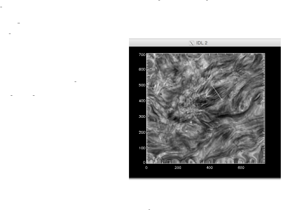
Figure 1: Hydrogen αline centre data set. The units are
in pixels and the white slit shows the location of the slit from
which the data for the time-distance diagram is extracted us-
ing diag slit. The slit is placed across a large-scale feature
composed of many fine-scale dark fibrils.
The diag slit.pro routine is a simple point and click
routine that lets you pick two data points, calculates
a straight line between the two points and extracts
the intensity values along the line via cubic inter-
polation, doing this for all time-frames in the data
cube.
A typical calling procedure for diag slit is:
IDL>diag slit,data cube,slit
where slit is the outputted time-distance diagram. In
Figure 1 a typical example of data selection is given and
the output shown is shown in Figure 2.
3 Wave tracking
The basic premise behind the wave tracking routine is
just a simple feature finding routine. The routine iden-
tifies peaks in intensity throughout the TD diagram of
interest. A peak is defined as the local maximum inten-
sity value in a search box, whose size can be set by the
user. The gradient of the slopes either side of the local
maximum are used to determine whether the found lo-
cal maximum is identified as a peak or not. The local
maximum is required to have a positive and negative
slope on the left and right hand side respectively. The
user also has to select the minimum value of the gradi-
ent of the slope, i.e., a cut-off value. This value is not
the same for different data sets and the user should test
different values for the gradient cut-off. A gradient too large selects no points, a gradient cut-off that is too small
ends up picking up the noise in the data, as well as the signal. The routine essentially scans through the TD
diagram, identifying all peaks that meet the criteria. NOTE: only positive peaks are found - so if your
interested in features that have lower intensities than the background (e.g., fibrils) you will need to
invert the intensities! (we typically multiply the TD by -1 and add back the maximum image value).
The routine has two modes for finding the location of the peaks, one more accurate than the other. The first mode
just takes the given location of maximum intensity at pixel level accuracy, and are given an error that is ±0.5 pixel.
This is a clearly a very coarse method.
Wave Tracking Documentation 3
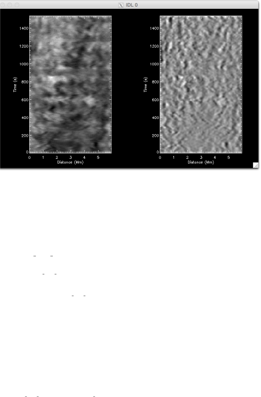
Figure 2: Time-distance-diagrams. The left hand panel shows the intensity time-distance diagram from the slit in Figure 1.
The right hand panel is an unsharp mask version of the same data, revealing more clearly the swaying of the dark fibrils.
The second mode is based on the least-squares fitting of a Gaussian function to the peak in intensity, allowing
for a sub-pixel estimate of the location of the intensity peak. This method inherently assumes that the intensity
uncertainties are approximately Normally distributed, which is largely the case for solar data dominated by photon
noise.
3.1 quick plot ft
The various wave tracking routines are made up of a number of smaller sub-routines that perform various tasks.
The routine quick plot ft is essentially a quick look routine, to test out how various input parameters influence the
location and fitting of intensity peaks.
The basic call is: IDL>quick plot ft,td
where td is the time-distance diagram to process. This call uses the basic method for peak finding. The user will
be prompted to input a gradient cut-off value. A suitable value of the gradient for different data sets will require
some trial and error. In Figure 3 we show the output from the routine (default plot to screen), the result is shown
for the case when the cut-off is far to restrictive, and no peaks have been selected. A better selection of the gradient
finds the structure, but doesn’t introduce too much noise into the found peaks, an example of which is shown in
Figure 4.
In Figure 4 there is clearly the influence of noise. The influence of noise can be reduced, e.g., by averaging, smooth-
ing, or a high-frequency noise filtering technique (Figure 5).
To test the second fitting method, the call is:
IDL>quick plot ft,td,/gauss,error=td er
Wave Tracking Documentation 4
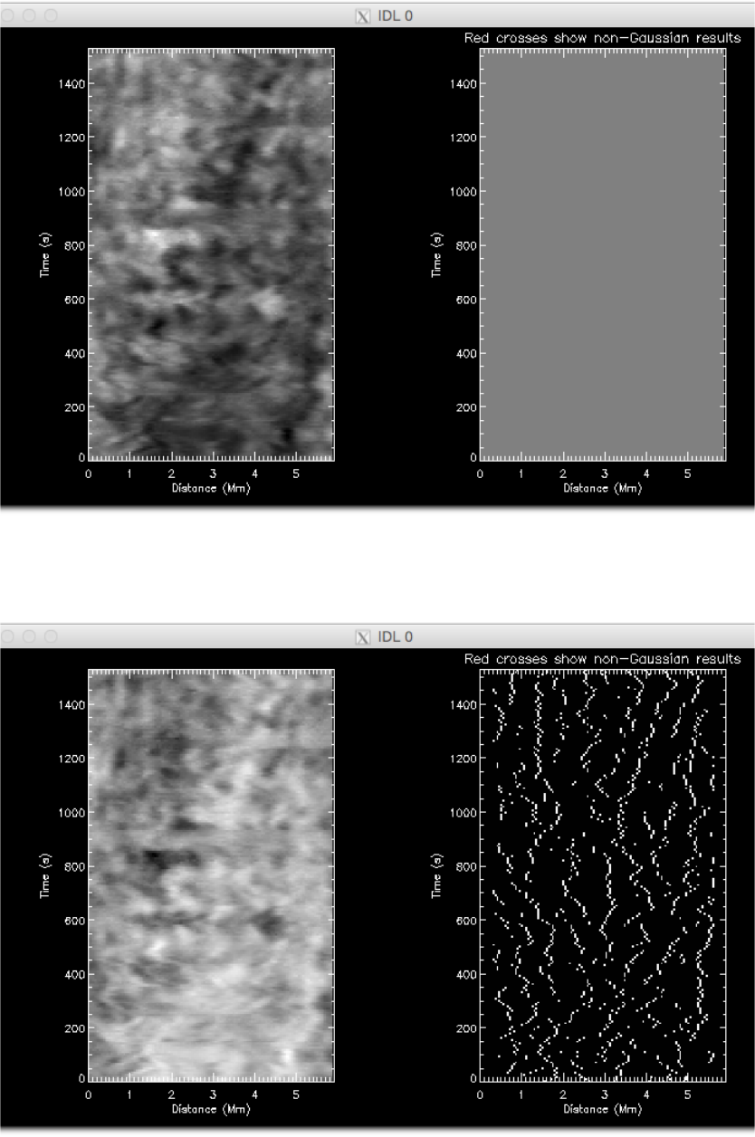
Figure 3: Peak finding. The left hand panel shows the intensity time-distance diagram. The right hand panel shows the
results of a harsh gradient constraint - nothing is found!
Figure 4: Peak finding. The left hand panel shows the intensity time-distance diagram. The right hand panel shows the
results of the peak location.
Wave Tracking Documentation 5
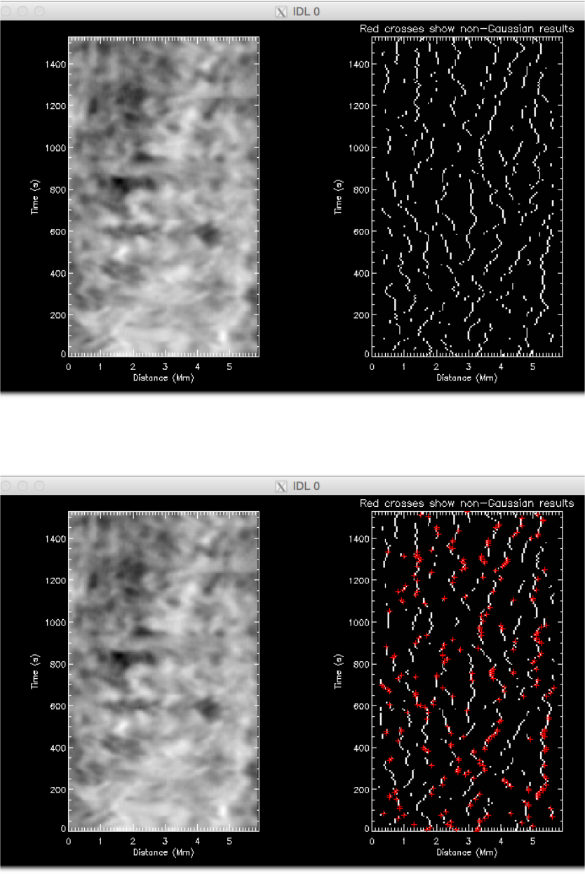
Figure 5: Peak finding. The left hand panel shows the intensity time-distance diagram. The right hand panel shows the
results of the peak location, with a smoothing of the TD diagram in the time-direction.
Figure 6: Peak finding. The left hand panel shows the intensity time-distance diagram. The right hand panel shows the
results of the peak location, using smoothed TD and the Gaussian peak location. The red crosses show where the Gaussian
fit was rejected and the basic peak location is used.
Wave Tracking Documentation 6
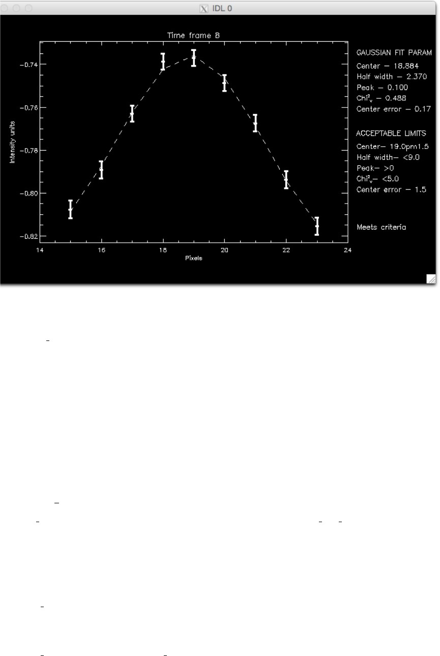
Figure 7: Example of fitted fibril cross-section.
Here, the td err is the uncertainties on the intensity values in the time-distance diagram. This should be calculated
by the user using, e.g., the properties of the instrument (sensor efficiency, gain, readout noise etc.). It should be
the same dimensions and size as td. The uncertainties are used to weight the Gaussian fit. They are required for
the code to run as it makes judgements about the goodness-of-fit of the Gaussian to the peak. If the peak doesn’t
meet the goodness-of-fit criteria, then the location of the peak is recorded using the basic properties, cf the first mode.
In Figure 6 the output window is shown for the Gaussian fitting. The red crosses show the locations where the fit
of the Gaussian failed to meet a list of criteria. For this example the assumed uncertainties of 0.5% of the intensity
value. NOTE: careful analysis of data uncertainties is highly recommended! Otherwise results will
not accurately reflect the uncertainties of the peak location.
There are a number of other keywords that lets you play with different parameters.
3.2 nuwt tr
The nuwt tr routine uses the same feature finding as discussed for quick plot ft. Once the peaks have been iden-
tified, an another sub-routine then ‘stitches’ together the peaks by crawling through the data. The routine starts
at a peak and searches forward in time for the next ‘local’ peak. The search box is 5 pixels in space by 4 in time.
If no pixel is found in the box, the thread is considered to be finished. The means small jumps in time are allowed for.
The basic calls for the routine are:
IDL>nuwt tr,data=td
or
IDL>nuwt tr,data=td,/gauss,error=td er
Here, data can be either one or many TD diagrams, in an array that is ordered as [x,t,n]. The user will be prompted
Wave Tracking Documentation 7

to enter a value for the gradient cut-off and also a minimum thread length. The routine will then reject any thread
whose length is less than that value. Further, any thread that has more than half of its value set to 0 will be
rejected. A window will be plotted to screen that shows the TD and the found peaks - there is no indication at this
stage of how many peak fittings failed for the Gaussian fit. Note, all peaks found are plotted - this image does not
reflect the threads found.
Once the fitting and stitching is complete, the user will be prompted as to whether they want to fit the threads. If
y, then the it takes you to an interactive fitting process, the details of which are given in the next sub-sub-section.
Answering nskips the fitting.
After the fitting stage, user is then asked whether they want the results to be saved. If yis chosen the you will be
prompted to enter a location to save the results. Once you have entered the information the routine will either quit
(if only one TD was input) or repeat (for many TD).
On opening the saved file, the user will find the outputs generated by the routine are saved as structures. Depending
on whether the threads where fitted or not, the saved outputs will either be threads or threads and threads fit.
The threads contains two extensions, threads.pos and threads.err pos, which give the measured location of the peaks
and the uncertainty on that position. Each array has the same time length as the original TD. The time frames
where no peak is found contain a −1. The remaining either contain the position value or a 0. The 0 corresponds
to time-frames that were jumped over at the crawling stage, i.e., no peak has been found between the time frames.
Note, it is up to the user to decide which found threads are worth using for further science.
If the user has used the internal fitting routine, then there will also be a structure called threads fit in the idl save
file. The saved data has three extensions, threads fit.pos,threads fit.err pos, and threads fit.fit result. The first two
extensions contain similar information to threads (although slightly modified - see wave fitting section for details).
The extension threads fit.fit result, predictably, contains the details related to the fitting (again, see fitting section
for more details).
3.3 Wave fitting
We have updated the wave fitting part of the routine to make it more flexible. Users can now write their own
function and pass this to nuwt tr via the user func and start keywords. We have provided the original functions
for fitting:
f(t) = A0+A1sin 2.πt
A2
−A3+tA4,(1)
f(t) = A0+A1sin 2.πt
A2
−A3exp(−A5t) + tA4,(2)
f(t) = A0+A1sin 2.πt
A2(1 + A6t)−A3exp(−A5t) + tA4.(3)
The function Eq. 1 is the default fitting option, the others can now be selected by the above keywords. To use a
non-default function you will need to provide the name of the function as a string and an array of estimates for the
parameters. The array is just used for initialisation purposes and values can be altered later. The call then looks
like (for model in Eq. 2)
IDL>nuwt tr,data=td, user func=’damped’, start = [0., 2., 100., 0., 0.01,1.]
Note, the function chosen at the start of the routine is used for fitting all threads found! (This is obviously restrictive
and we are looking to improve this aspect).
Once the fitting section of the routine has been entered, the routine performs a gap-filling. Any threads that have
zero’s in it’s entries are filled. The default option for the filling is to give the blank entry the same value as found
for the previous entry in the array and assigning it an error of ±1 pixel. The large value of the error than essentially
gives the filled location less weight in the weighted lease squares. It is these filled arrays that are then saved in
threads fit.pos and threads fit.err pos. This fill assumes that the wave doesn’t move more than 1 pixel between
Wave Tracking Documentation 8

time-frames - how reasonable this is depends on what type of events you are measuring.
The routine will then show you which thread you are fitting, printing some text to the terminal and plotting the
thread to screen. From here, there are a number of options for user interaction via the terminal. You will first be
asked whether you would like to fit this thread. Answering nmoves on to the next thread. Answering y, you will
then be asked if you want to change the start and end positions of the thread. This allows you focus on fitting
certain portions of the thread. Answering nmoves on to the next step. Answering yshows you the current values
of time-frames it is fitting between and ask you to enter new tand t1 values, e.g.,
Fit this thread? - y/n y
Change start end of thread? - y/n y
Current value of t= 1 and t1= 20
Enter t value: 2
Enter t1 value: 17
After this, you will then be prompted about whether you want to subtract a polynomial trend line. Answering n
will skip this section. Selecting ywill then prompt you to enter the degree of the polynomial you wish to remove.
After entering a number, a polynomial is fit to the thread and removed, with the window updated with the new
thread. The χ2value of the fit is printed to screen for reference.
Change polynomial degree? - y/n y
Fit trend - enter polynomial degree: 2
Chiˆ2 of fit 10.7489
Is the fit good? y/n
If you are happy with the subtracted polynomial then answer y. Answering nrepeats the polynomial selection
again. Note: the removal of a polynomial trend before the fitting of the sinusoid will impact upon
the estimated uncertainties on the fitted parameters of the sinusoid, usually underestimating the
uncertainties. In reality, the polynomial terms should be fit with the sinusoid, rather than individ-
ually.
The next section of the routine begins the fitting of the selected function (Eq. 1-3). The fitting is performed with a
Levenberg-Marquadt algorithim (mpfit.pro - cite), which requires initial guesses for the parameters to be fit. The
routine has a default parameter range set, but this will likely be unsuitable for most cases. The user will be asked
whether the initial variables should be changed, selecting ntries the default initial values while selecting ylets you
change the start values for amplitude and period (Note, in our experience we have found that the initial values for
period and amplitude have the greatest impact on the fit, hence they are the only variables allowed to change.):
Initial variables: Constant=43.0000 Amplitude=1.00000 Period=20.0000 Phase=0.500000 Linear=1.00000
Change initial variables? y/n y
Enter amplitude: 2.
Enter period: 15.
%
%
Fitted variables 3.33458 68.1474 75.1892 -2.55123 4.85452
Error on fits 126.310 320.733 122.048 0.929392 17.6052
Chiˆ2 75.1915
Repeat fitting procedure? - y/n
The fit is overplotted in the window. Should you be unhappy with the fit, selecting ystarts the process again from
the selection of time-frames. This process can be repeated as many times as desired. Selecting nthen ends the
fitting of the current thread. You are then prompted whether to save the results of the fitting. Selecting ywill
record the fit parameters in threads fit.fit result, selecting nwill not record the values. The routine then moves onto
the next thread.
As mentioned, the results of the fit are stored in threads fit.fit result. For an nparameter fit, array entries corre-
Wave Tracking Documentation 9

spond to:
fit result[0:n-1] - parameters
fit result[n:2n-1] - formal 1 sigma errors on parameters
fit result[2n]=chiˆ2 for fit
fit result[2n+1]=start time from start of time-distance diagram
fit result[2n+2]=end time
fit result[2n+3]=pre-fitting used; (1)-non (2,3....)- polynomial degree
4 To do
The following is a list of future upgrades that may be implemented. This list is not exclusive and will be updated.
If you find bugs or have suggestions, they can be added to the list. Further, if anybody would like to work on any
of these issues please feel free!! We will be running the code through Git, so version control will be in place.
•Update χ2cut-off for Gaussian fitting of cross-section - At present, reduced χ2is used and set to a hard value
of 5. This should be either set by a critical value for rejection. However, reduced χ2is not an appropriate
measure for goodness of fit for non-linear functions (cite), so implementing a Kolmogorov-Smirnov test may
provide greater confidence.
•Improve flexibility of fitting routine further.
Wave Tracking Documentation 10
