Tektronix Signal_integrity Signal Integrity
User Manual: signal_integrity Tektronix Oscilloscope Use
Open the PDF directly: View PDF ![]() .
.
Page Count: 7
www.tektronix.com
4
Signal Integrity
The Significance of Signal Integrity
The key to any good oscilloscope system is its ability to accurately recon-
struct a waveform – referred to as signal integrity. An oscilloscope is
analogous to a camera that captures signal images that we can then
observe and interpret. Two key issues lie at the heart of signal integrity.
When you take a picture, is it an accurate picture of what actually happened?
Is the picture clear or fuzzy?
How many of those accurate pictures can you take per second?
Taken together, the different systems and performance capabilities of an
oscilloscope contribute to its ability to deliver the highest signal integrity
possible. Probes also affect the signal integrity of a measurement system.
Signal integrity impacts many electronic design disciplines. But until a
few years ago, it wasn’t much of a problem for digital designers. They
could rely on their logic designs to act like the Boolean circuits they were.
Noisy, indeterminate signals were something that occurred in high-speed
designs – something for RF designers to worry about. Digital systems
switched slowly and signals stabilized predictably.
Processor clock rates have since multiplied by orders of magnitude.
Computer applications such as 3D graphics, video and server I/O
demand vast bandwidth. Much of today’s telecommunications equipment
is digitally based, and similarly requires massive bandwidth. So too
does digital high-definition TV.The current crop of microprocessor
devices handles data at rates up to 2, 3 and even 5 GS/s (gigasamples per
second), while some memory devices use 400-MHz clocks as well as data
signals with 200-ps rise times.
Importantly, speed increases have trickled down to the common IC
devices used in automobiles, VCRs, and machine controllers, to name
just a few applications. A processor running at a 20-MHz clock rate
may well have signals with rise times similar to those of an 800-MHz
processor. Designers have crossed a performance threshold that means,
in effect, almost every design is a high-speed design.
Without some precautionary measures, high-speed problems can
creep into otherwise conventional digital designs. If a circuit is
experiencing intermittent failures, or if it encounters errors at voltage
and temperature extremes, chances are there are some hidden signal
integrity problems. These can affect time-to-market, product reliability,
EMI compliance, and more.
Why is Signal Integrity a Problem?
Let’s look at some of the specific causes of signal degradation in today’s
digital designs. Why are these problems so much more prevalent today
than in years past?
The answer is speed. In the “slow old days,” maintaining acceptable
digital signal integrity meant paying attention to details like clock
distribution, signal path design, noise margins, loading effects,
transmission line effects, bus termination, decoupling and power
distribution. All of these rules still apply, but…
Bus cycle times are up to a thousand times faster than they were
20 years ago! Transactions that once took microseconds are now
measured in nanoseconds. To achieve this improvement, edge speeds
too have accelerated: they are up to 100 times faster than those of
two decades ago.
This is all well and good; however, certain physical realities have kept
circuit board technology from keeping up the pace. The propagation time
of inter-chip buses has remained almost unchanged over the decades.
Geometries have shrunk, certainly, but there is still a need to provide
circuit board real estate for IC devices, connectors, passive components,
and of course, the bus traces themselves. This real estate adds up to
distance, and distance means time – the enemy of speed.
It’s important to remember that the edge speed – rise time – of a digital
signal can carry much higher frequency components than its repetition
rate might imply. For this reason, some designers deliberately seek IC
devices with relatively “slow” rise times.
XYZs of Oscilloscopes
Primer
www.tektronix.com 5
The lumped circuit model has always been the basis of most calculations
used to predict signal behavior in a circuit. But when edge speeds are
more than four to six times faster than the signal path delay, the simple
lumped model no longer applies.
Circuit board traces just six inches long become transmission lines
when driven with signals exhibiting edge rates below four to six
nanoseconds, irrespective of the cycle rate. In effect, new signal paths
are created. These intangible connections aren’t on the schematics, but
nevertheless provide a means for signals to influence one another in
unpredictable ways.
At the same time, the intended signal paths don’t work the way they
are supposed to. Ground planes and power planes, like the signal
traces described above, become inductive and act like transmission
lines; power supply decoupling is far less effective. EMI goes up as
faster edge speeds produce shorter wavelengths relative to the bus
length. Crosstalk increases.
In addition, fast edge speeds require generally higher currents to produce
them. Higher currents tend to cause ground bounce, especially on wide
buses in which many signals switch at once. Moreover, higher current
increases the amount of radiated magnetic energy and with it, crosstalk.
Viewing the Analog Origins of Digital Signals
What do all these characteristics have in common? They are classic
analog phenomena. To solve signal integrity problems, digital designers
need to step into the analog domain. And to take that step, they need
tools that can show them how digital and analog signals interact.
Digital errors often have their roots in analog signal integrity problems.
To track down the cause of the digital fault, it’s often necessary to turn
to an oscilloscope, which can display waveform details, edges and noise;
can detect and display transients; and can help you precisely measure
timing relationships such as setup and hold times.
Understanding each of the systems within your oscilloscope and how to
apply them will contribute to the effective application of the oscilloscope
to tackle your specific measurement challenge.
The Oscilloscope
What is an oscilloscope and how does it work? This section answers
these fundamental questions.
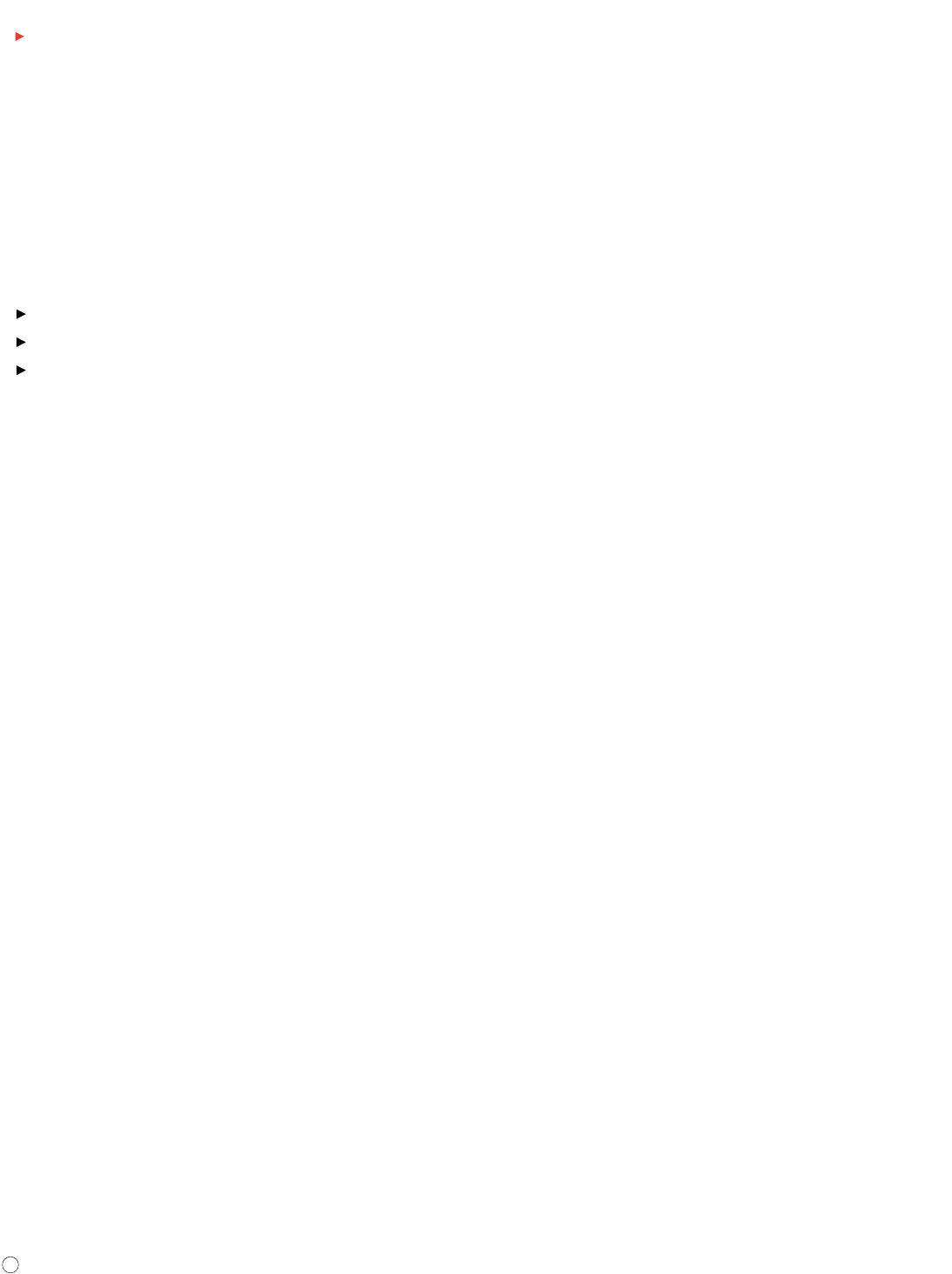
The oscilloscope is basically a graph-displaying device – it draws a
graph of an electrical signal. In most applications, the graph shows how
signals change over time: the vertical (Y) axis represents voltage and the
horizontal (X) axis represents time. The intensity or brightness of the
display is sometimes called the Z axis. (See Figure 2.)
This simple graph can tell you many things about a signal, such as:
The time and voltage values of a signal
The frequency of an oscillating signal
The “moving parts” of a circuit represented by the signal
The frequency with which a particular portion of the signal is occurring relative to
other portions
Whether or not a malfunctioning component is distorting the signal
How much of a signal is direct current (DC) or alternating current (AC)
How much of the signal is noise and whether the noise is changing with time
XYZs of Oscilloscopes
Primer
Z (intensity)
Y (voltage)
X (time)
Y (voltage)
X (time)
Z (intensity)
Figure 2. X, Y, and Z components of a displayed waveform.
www.tektronix.com
6
Understanding Waveforms and
Waveform Measurements
The generic term for a pattern that repeats over time is a wave – sound
waves, brain waves, ocean waves, and voltage waves are all repetitive
patterns. An oscilloscope measures voltage waves. One cycle of a wave
is the portion of the wave that repeats. A waveform is a graphic
representation of a wave. A voltage waveform shows time on the
horizontal axis and voltage on the vertical axis.
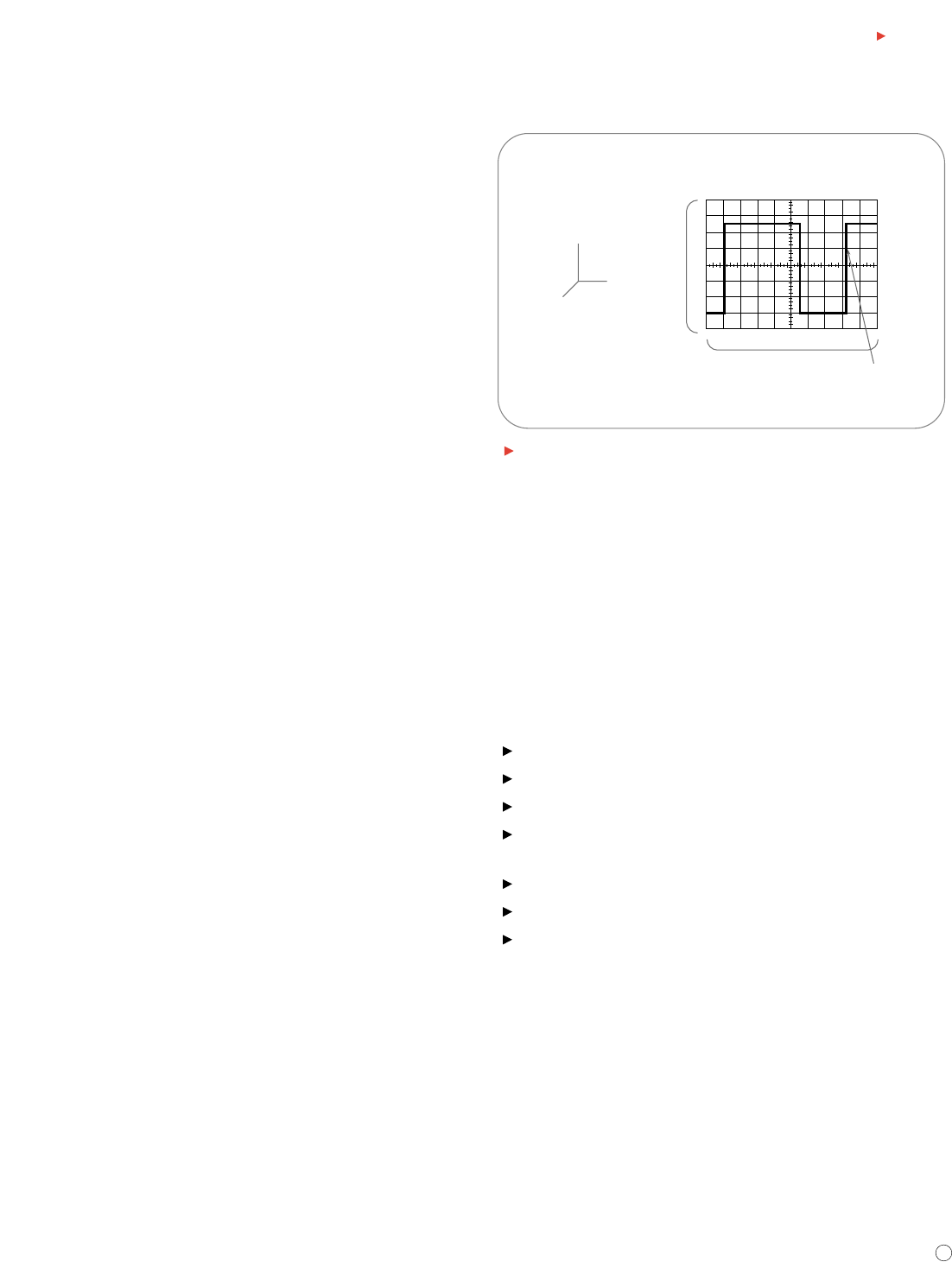
Waveform shapes reveal a great deal about a signal. Any time you see
a change in the height of the waveform, you know the voltage has
changed. Any time there is a flat horizontal line, you know that there
is no change for that length of time. Straight, diagonal lines mean a
linear change – rise or fall of voltage at a steady rate. Sharp angles on
a waveform indicate sudden change. Figure 3 shows common waveforms
and Figure 4 displays sources of common waveforms.
XYZs of Oscilloscopes
Primer
Sine Wave Damped Sine Wave
Square Wave Rectangular Wave
Sawtooth Wave Triangle Wave
Step Pulse
Complex
Figure 3. Common waveforms.
Figure 4. Sources of common waveforms.
www.tektronix.com 7
Types of Waves
You can classify most waves into these types:
Sine waves
Square and rectangular waves
Triangle and saw-tooth waves
Step and pulse shapes
Periodic and non-periodic signals
Synchronous and asynchronous signals
Complex waves
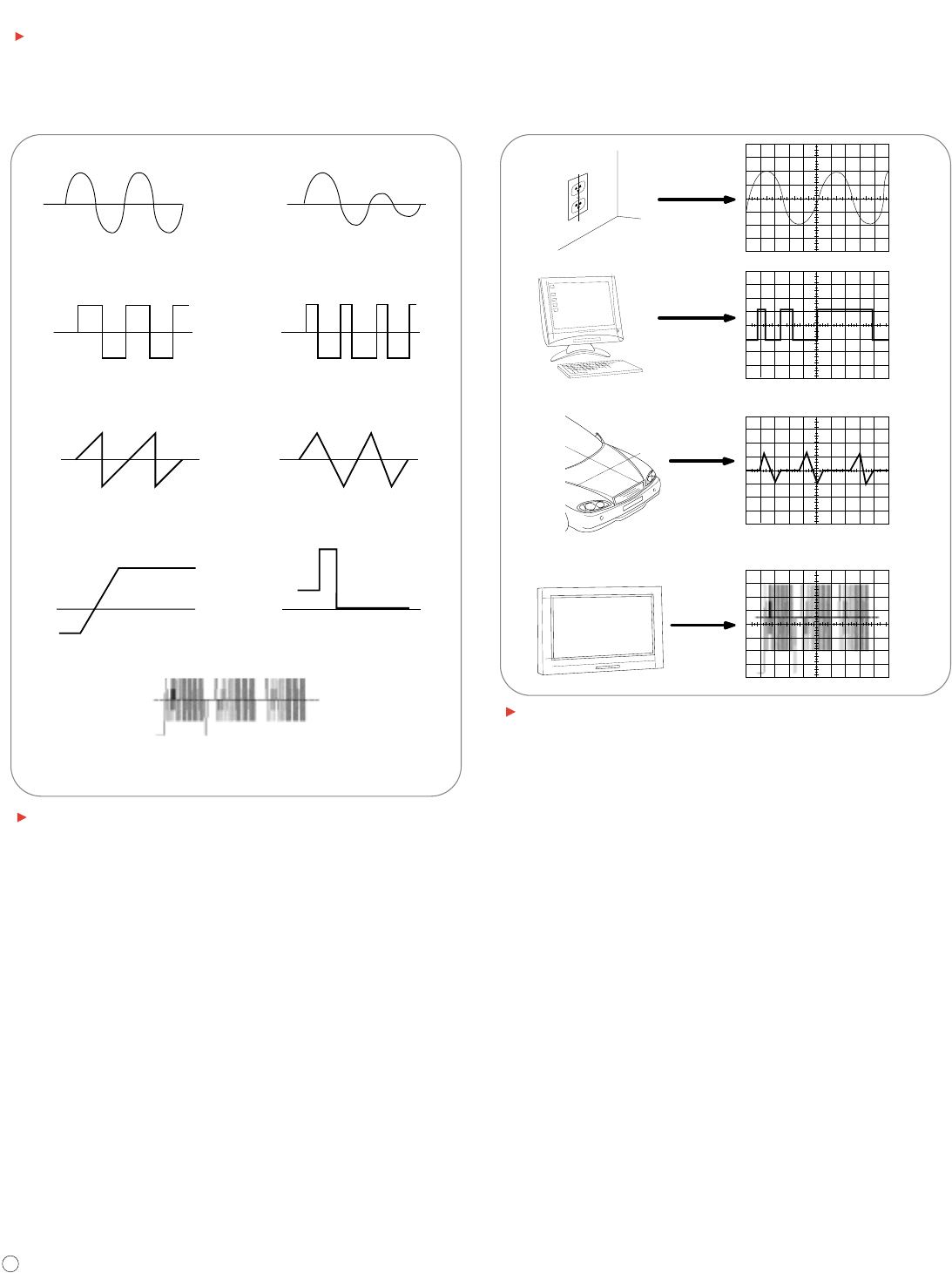
Sine Waves
The sine wave is the fundamental wave shape for several reasons. It has
harmonious mathematical properties – it is the same sine shape you may
have studied in high school trigonometry class. The voltage in your wall
outlet varies as a sine wave. Test signals produced by the oscillator circuit
of a signal generator are often sine waves. Most AC power sources pro-
duce sine waves. (AC signifies alternating current, although the voltage
alternates too. DC stands for direct current, which means a steady current
and voltage, such as a battery produces.)
The damped sine wave is a special case you may see in a circuit that
oscillates, but winds down over time. Figure 5 shows examples of sine and
damped sine waves.
Square and Rectangular Waves
The square wave is another common wave shape. Basically, a square
wave is a voltage that turns on and off (or goes high and low) at regular
intervals. It is a standard wave for testing amplifiers – good amplifiers
increase the amplitude of a square wave with minimum distortion.
Television, radio and computer circuitry often use square waves for
timing signals.
The rectangular wave is like the square wave except that the high and
low time intervals are not of equal length. It is particularly important when
analyzing digital circuitry. Figure 6 shows examples of square and
rectangular waves.
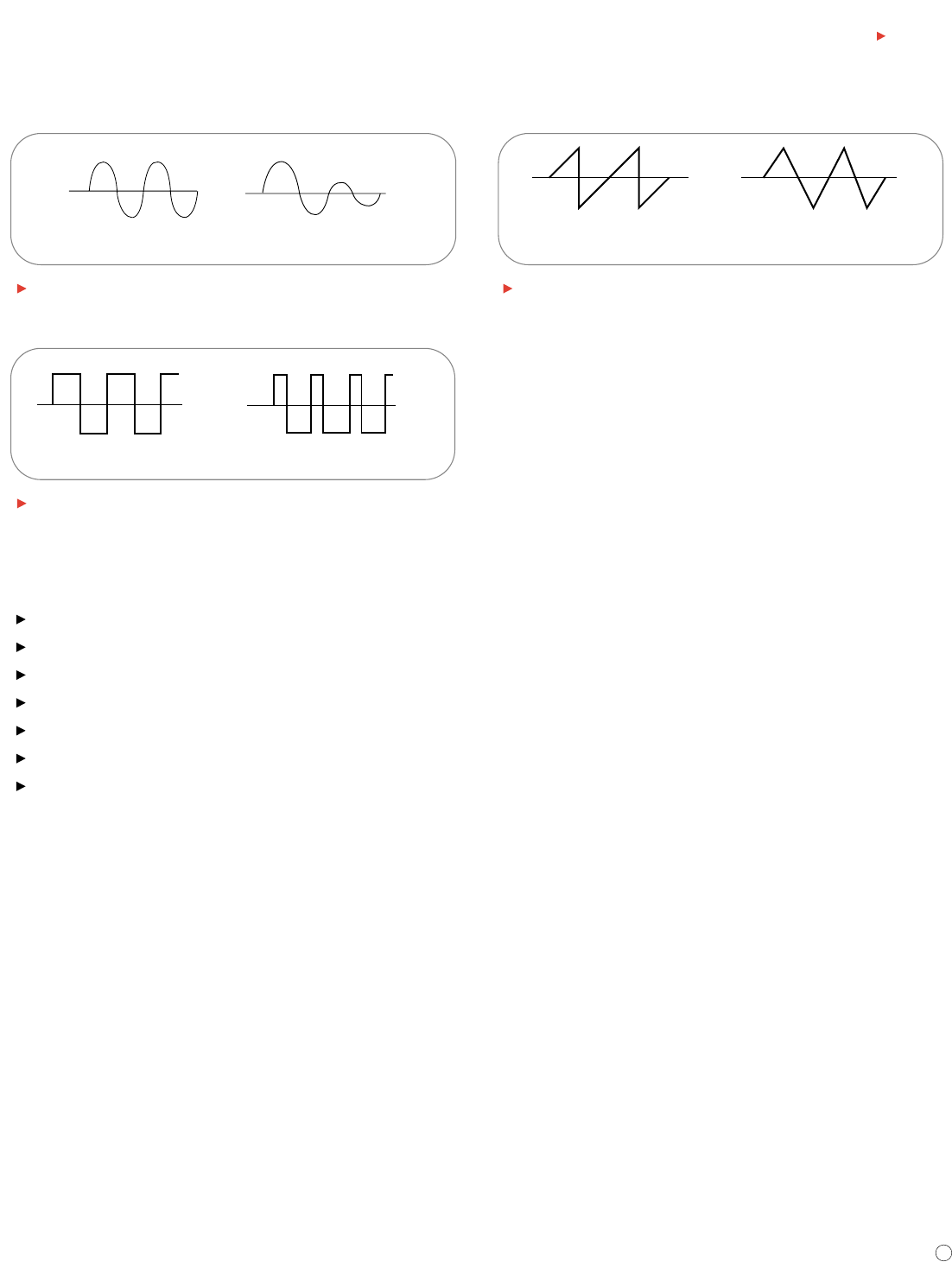
Sawtooth and Triangle Waves
Sawtooth and triangle waves result from circuits designed to control
voltages linearly, such as the horizontal sweep of an analog oscilloscope or
the raster scan of a television. The transitions between voltage levels of
these waves change at a constant rate. These transitions are called
ramps. Figure 7 shows examples of saw-tooth and triangle waves.
XYZs of Oscilloscopes
Primer
Sawtooth Wave Triangle Wave
Figure 7. Sawtooth and triangle waves.
Sine Wave Damped Sine Wave
Figure 5. Sine and damped sine waves.
Square Wave Rectangular Wave
Figure 6. Square and rectangular waves.
www.tektronix.com
8
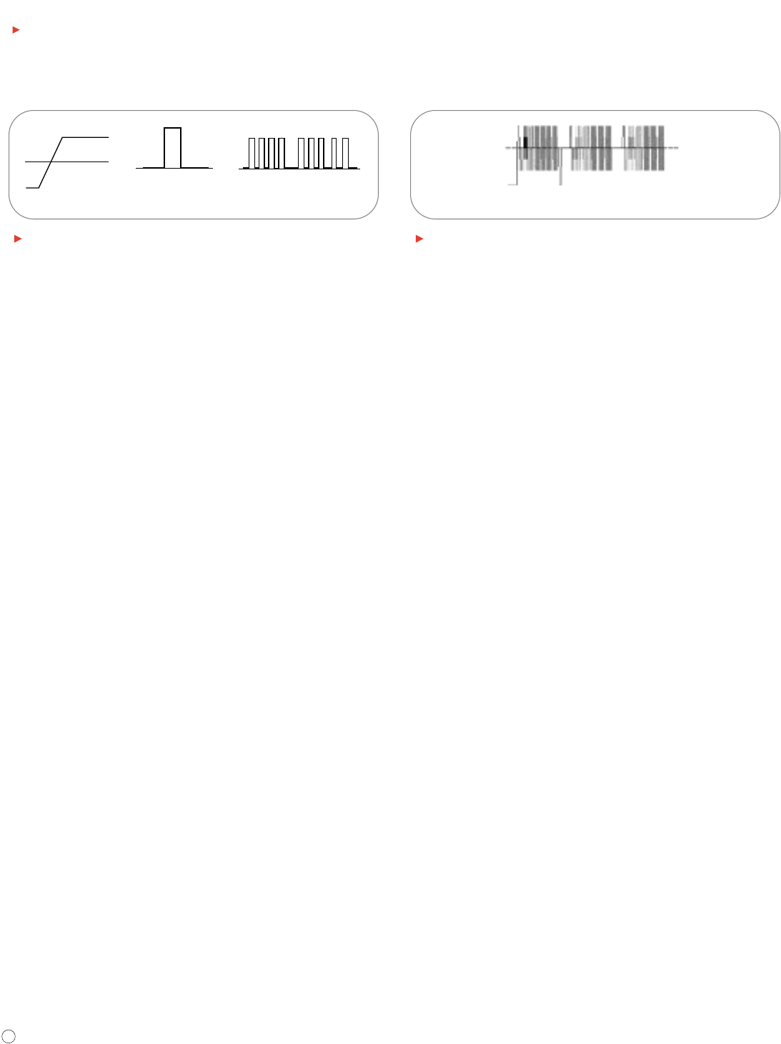
Step and Pulse Shapes
Signals such as steps and pulses that occur rarely, or non-periodically,
are called single-shot or transient signals. A step indicates a sudden
change in voltage, similar to the voltage change you would see if you
turned on a power switch.
A pulse indicates sudden changes in voltage, similar to the voltage
changes you would see if you turned a power switch on and then off
again. A pulse might represent one bit of information traveling through
a computer circuit or it might be a glitch, or defect, in a circuit. A
collection of pulses traveling together creates a pulse train. Digital
components in a computer communicate with each other using pulses.
Pulses are also common in x-ray and communications equipment.
Figure 8 shows examples of step and pulse shapes and a pulse train.
Periodic and Non-periodic Signals
Repetitive signals are referred to as periodic signals, while signals that
constantly change are known as non-periodic signals. A still picture is
analogous to a periodic signal, while a moving picture can be equated to
a non-periodic signal.
Synchronous and Asynchronous Signals
When a timing relationship exists between two signals, those signals are
referred to as synchronous. Clock, data and address signals inside a
computer are an example of synchronous signals.
Asynchronous is a term used to describe those signals between which no
timing relationship exists. Because no time correlation exists between the
act of touching a key on a computer keyboard and the clock inside the
computer, these are considered asynchronous.
Complex Waves
Some waveforms combine the characteristics of sines, squares, steps,
and pulses to produce waveshapes that challenge many oscilloscopes.
The signal information may be embedded in the form of amplitude, phase,
and/or frequency variations. For example, although the signal in Figure 9
is an ordinary composite video signal, it is composed of many cycles of
higher-frequency waveforms embedded in a lower-frequency envelope.
In this example, it is usually most important to understand the relative
levels and timing relationships of the steps. To view this signal, you need
an oscilloscope that captures the low-frequency envelope and blends in
the higher-frequency waves in an intensity-graded fashion so that you can
see their overall combination as an image that can be visually interpreted.
Analog and digital phosphor oscilloscopes are most suited to viewing
complex waves, such as video signals, illustrated in Figure 9. Their
displays provide the necessary frequency-of-occurrence information, or
intensity grading, that is essential to understanding what the waveform
is really doing.
XYZs of Oscilloscopes
Primer
Complex
Figure 9. An NTSC composite video signal is an example of a complex wave.
Step Pulse Pulse Train
Figure 8. Step, pulse and pulse train shapes.
www.tektronix.com 9
Waveform Measurements
Many terms are used to describe the types of measurements that you
make with your oscilloscope. This section describes some of the most
common measurements and terms.
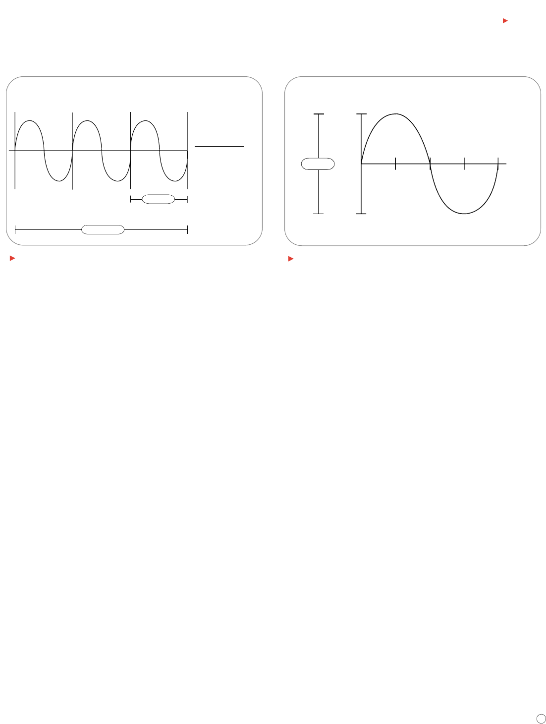
Frequency and Period
If a signal repeats, it has a frequency.The frequency is measured in
Hertz (Hz) and equals the number of times the signal repeats itself in
one second, referred to as cycles per second. A repetitive signal also
has a period – this is the amount of time it takes the signal to complete
one cycle. Period and frequency are reciprocals of each other, so that
1/period equals the frequency and 1/frequency equals the period. For
example, the sine wave in Figure 10 has a frequency of 3 Hz and a period
of 1/3 second.
Voltage
Voltage is the amount of electric potential – or signal strength – between
two points in a circuit. Usually, one of these points is ground, or zero
volts, but not always. You may want to measure the voltage from the
maximum peak to the minimum peak of a waveform, referred to as the
peak-to-peak voltage.
Amplitude
Amplitude refers to the amount of voltage between two points in a circuit.
Amplitude commonly refers to the maximum voltage of a signal measured
from ground, or zero volts. The waveform shown in Figure 11 has an
amplitude of 1 V and a peak-to-peak voltage of 2 V.
XYZs of Oscilloscopes
Primer
0°90°180°270°360
+1 V
–1 V
0
2 V
°
Figure 11. Amplitude and degrees of a sine wave.
period
1 second
3 Cycles per
Second = 3 Hz
Frequency
123
Figure 10. Frequency and period of a sine wave.
www.tektronix.com
10
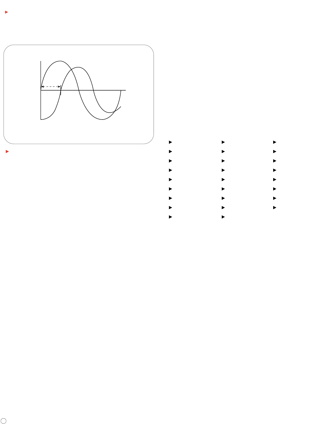
Phase
Phase is best explained by looking at a sine wave. The voltage level of
sine waves is based on circular motion. Given that a circle has 360°, one
cycle of a sine wave has 360°, as shown in Figure 11. Using degrees, you
can refer to the phase angle of a sine wave when you want to describe
how much of the period has elapsed.
Phase shift describes the difference in timing between two otherwise sim-
ilar signals. The waveform in Figure 12 labeled “current” is said to be 90°
out of phase with the waveform labeled “voltage,” since the waves reach
similar points in their cycles exactly 1/4 of a cycle apart (360°/4 = 90°).
Phase shifts are common in electronics.
Waveform Measurements with Digital Oscilloscopes
Modern digital oscilloscopes have functions that make waveform
measurements easier. They have front-panel buttons and/or screen-based
menus from which you can select fully automated measurements. These
include amplitude, period, rise/fall time, and many more. Many digital
instruments also provide mean and RMS calculations, duty cycle, and
other math operations. Automated measurements appear as on-screen
alphanumeric readouts. Typically these readings are more accurate
than is possible to obtain with direct graticule interpretation.
Fully automated waveform measurements available on some
digital phosphor oscilloscopes include:
Period Duty cycle + High
Frequency Duty cycle – Low
Width + Delay Minimum
Width – Phase Maximum
Rise time Burst width Overshoot +
Fall time Peak-to-peak Overshoot –
Amplitude Mean RMS
Extinction ratio Cycle mean Cycle RMS
Mean optical power Cycle area
XYZs of Oscilloscopes
Primer
0
Phase = 90°
Voltage
Current
Figure 12. Phase shift.
