Prml Web Sol.dvi Solution Manual
solution%20manual
User Manual:
Open the PDF directly: View PDF ![]() .
.
Page Count: 101 [warning: Documents this large are best viewed by clicking the View PDF Link!]


Pattern Recognition and Machine Learning
Solutions to the Exercises: Web-Edition
Markus Svens´
en and Christopher M. Bishop
Copyright c
2002–2009
This is the solutions manual (web-edition) for the book Pattern Recognition and Machine Learning
(PRML; published by Springer in 2006). It contains solutions to the www exercises. This release
was created September 8, 2009. Future releases with corrections to errors will be published on the PRML
web-site (see below).
The authors would like to express their gratitude to the various people who have provided feedback on
earlier releases of this document. In particular, the “Bishop Reading Group”, held in the Visual Geometry
Group at the University of Oxford provided valuable comments and suggestions.
The authors welcome all comments, questions and suggestions about the solutions as well as reports on
(potential) errors in text or formulae in this document; please send any such feedback to
prml-fb@microsoft.com
Further information about PRML is available from
http://research.microsoft.com/∼cmbishop/PRML
Contents
Contents 5
Chapter 1: Introduction . . . . . . . . . . . . . . . . . . . . . . . . . . . 7
Chapter 2: Probability Distributions . . . . . . . . . . . . . . . . . . . . 20
Chapter 3: Linear Models for Regression . . . . . . . . . . . . . . . . . . 35
Chapter 4: Linear Models for Classification . . . . . . . . . . . . . . . . 41
Chapter 5: Neural Networks . . . . . . . . . . . . . . . . . . . . . . . . 46
Chapter 6: Kernel Methods . . . . . . . . . . . . . . . . . . . . . . . . . 54
Chapter 7: Sparse Kernel Machines . . . . . . . . . . . . . . . . . . . . . 59
Chapter 8: Graphical Models . . . . . . . . . . . . . . . . . . . . . . . . 63
Chapter 9: Mixture Models and EM . . . . . . . . . . . . . . . . . . . . 68
Chapter 10: Approximate Inference . . . . . . . . . . . . . . . . . . . . . 72
Chapter 11: Sampling Methods . . . . . . . . . . . . . . . . . . . . . . . 83
Chapter 12: Continuous Latent Variables . . . . . . . . . . . . . . . . . . 85
Chapter 13: Sequential Data . . . . . . . . . . . . . . . . . . . . . . . . 92
Chapter 14: Combining Models . . . . . . . . . . . . . . . . . . . . . . . 97
5
6CONTENTS

Solutions 1.1–1.4 7
Chapter 1 Introduction
1.1 Substituting (1.1) into (1.2) and then differentiating with respect to wiwe obtain
N
X
n=1 M
X
j=0
wjxj
n−tn!xi
n= 0.(1)
Re-arranging terms then gives the required result.
1.4 We are often interested in finding the most probable value for some quantity. In
the case of probability distributions over discrete variables this poses little problem.
However, for continuous variables there is a subtlety arising from the nature of prob-
ability densities and the way they transform under non-linear changes of variable.
Consider first the way a function f(x)behaves when we change to a new variable y
where the two variables are related by x=g(y). This defines a new function of y
given by
e
f(y) = f(g(y)).(2)
Suppose f(x)has a mode (i.e. a maximum) at bxso that f(bx)=0. The correspond-
ing mode of e
f(y)will occur for a value byobtained by differentiating both sides of
(2) with respect to y
e
f(by) = f(g(by))g(by) = 0.(3)
Assuming g(by)6= 0 at the mode, then f(g(by)) = 0. However, we know that
f(bx) = 0, and so we see that the locations of the mode expressed in terms of each
of the variables xand yare related by bx=g(by), as one would expect. Thus, finding
a mode with respect to the variable xis completely equivalent to first transforming
to the variable y, then finding a mode with respect to y, and then transforming back
to x.
Now consider the behaviour of a probability density px(x)under the change of vari-
ables x=g(y), where the density with respect to the new variable is py(y)and is
given by ((1.27)). Let us write g(y) = s|g(y)|where s∈ {−1,+1}. Then ((1.27))
can be written
py(y) = px(g(y))sg(y).
Differentiating both sides with respect to ythen gives
p
y(y) = sp
x(g(y)){g(y)}2+spx(g(y))g(y).(4)
Due to the presence of the second term on the right hand side of (4) the relationship
bx=g(by)no longer holds. Thus the value of xobtained by maximizing px(x)will
not be the value obtained by transforming to py(y)then maximizing with respect to
yand then transforming back to x. This causes modes of densities to be dependent
on the choice of variables. In the case of linear transformation, the second term on
8Solution 1.7
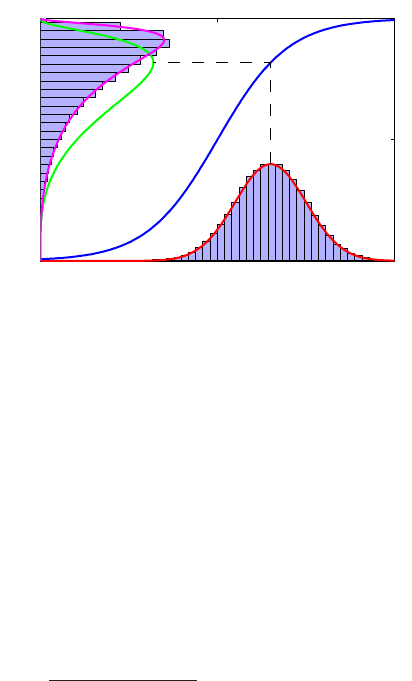
Figure 1 Example of the transformation of
the mode of a density under a non-
linear change of variables, illus-
trating the different behaviour com-
pared to a simple function. See the
text for details.
0 5 10
0
0.5
1
g−1(x)
px(x)
py(y)
y
x
the right hand side of (4) vanishes, and so the location of the maximum transforms
according to bx=g(by).
This effect can be illustrated with a simple example, as shown in Figure 1. We
begin by considering a Gaussian distribution px(x)over xwith mean µ= 6 and
standard deviation σ= 1, shown by the red curve in Figure 1. Next we draw a
sample of N= 50,000 points from this distribution and plot a histogram of their
values, which as expected agrees with the distribution px(x).
Now consider a non-linear change of variables from xto ygiven by
x=g(y) = ln(y)−ln(1 −y) + 5.(5)
The inverse of this function is given by
y=g−1(x) = 1
1 + exp(−x+ 5) (6)
which is a logistic sigmoid function, and is shown in Figure 1 by the blue curve.
If we simply transform px(x)as a function of xwe obtain the green curve px(g(y))
shown in Figure 1, and we see that the mode of the density px(x)is transformed
via the sigmoid function to the mode of this curve. However, the density over y
transforms instead according to (1.27) and is shown by the magenta curve on the left
side of the diagram. Note that this has its mode shifted relative to the mode of the
green curve.
To confirm this result we take our sample of 50,000 values of x, evaluate the corre-
sponding values of yusing (6), and then plot a histogram of their values. We see that
this histogram matches the magenta curve in Figure 1 and not the green curve!
1.7 The transformation from Cartesian to polar coordinates is defined by
x=rcos θ(7)
y=rsin θ(8)

Solution 1.8 9
and hence we have x2+y2=r2where we have used the well-known trigonometric
result (2.177). Also the Jacobian of the change of variables is easily seen to be
∂(x, y)
∂(r, θ)=
∂x
∂r
∂x
∂θ
∂y
∂r
∂y
∂θ
=cos θ−rsin θ
sin θ r cos θ=r
where again we have used (2.177). Thus the double integral in (1.125) becomes
I2=Z2π
0Z∞
0
exp −r2
2σ2rdrdθ(9)
= 2πZ∞
0
exp −u
2σ21
2du(10)
=πhexp −u
2σ2−2σ2i∞
0(11)
= 2πσ2(12)
where we have used the change of variables r2=u. Thus
I=2πσ21/2.
Finally, using the transformation y=x−µ, the integral of the Gaussian distribution
becomes Z∞
−∞ Nx|µ, σ2dx=1
(2πσ2)1/2Z∞
−∞
exp −y2
2σ2dy
=I
(2πσ2)1/2= 1
as required.
1.8 From the definition (1.46) of the univariate Gaussian distribution, we have
E[x] = Z∞
−∞ 1
2πσ21/2
exp −1
2σ2(x−µ)2xdx. (13)
Now change variables using y=x−µto give
E[x] = Z∞
−∞ 1
2πσ21/2
exp −1
2σ2y2(y+µ) dy. (14)
We now note that in the factor (y+µ)the first term in ycorresponds to an odd
integrand and so this integral must vanish (to show this explicitly, write the integral

10 Solution 1.9
as the sum of two integrals, one from −∞ to 0and the other from 0to ∞and then
show that these two integrals cancel). In the second term, µis a constant and pulls
outside the integral, leaving a normalized Gaussian distribution which integrates to
1, and so we obtain (1.49).
To derive (1.50) we first substitute the expression (1.46) for the normal distribution
into the normalization result (1.48) and re-arrange to obtain
Z∞
−∞
exp −1
2σ2(x−µ)2dx=2πσ21/2.(15)
We now differentiate both sides of (15) with respect to σ2and then re-arrange to
obtain 1
2πσ21/2Z∞
−∞
exp −1
2σ2(x−µ)2(x−µ)2dx=σ2(16)
which directly shows that
E[(x−µ)2] = var[x] = σ2.(17)
Now we expand the square on the left-hand side giving
E[x2]−2µE[x] + µ2=σ2.
Making use of (1.49) then gives (1.50) as required.
Finally, (1.51) follows directly from (1.49) and (1.50)
E[x2]−E[x]2=µ2+σ2−µ2=σ2.
1.9 For the univariate case, we simply differentiate (1.46) with respect to xto obtain
d
dxNx|µ, σ2=−N x|µ, σ2x−µ
σ2.
Setting this to zero we obtain x=µ.
Similarly, for the multivariate case we differentiate (1.52) with respect to xto obtain
∂
∂xN(x|µ,Σ) = −1
2N(x|µ,Σ)∇x(x−µ)TΣ−1(x−µ)
=−N(x|µ,Σ)Σ−1(x−µ),
where we have used (C.19), (C.20)1and the fact that Σ−1is symmetric. Setting this
derivative equal to 0, and left-multiplying by Σ, leads to the solution x=µ.
1NOTE: In the 1st printing of PRML, there are mistakes in (C.20); all instances of x(vector)
in the denominators should be x(scalar).

Solutions 1.10–1.12 11
1.10 Since xand zare independent, their joint distribution factorizes p(x, z) = p(x)p(z),
and so
E[x+z] = ZZ(x+z)p(x)p(z) dxdz(18)
=Zxp(x) dx+Zzp(z) dz(19)
=E[x] + E[z].(20)
Similarly for the variances, we first note that
(x+z−E[x+z])2= (x−E[x])2+ (z−E[z])2+ 2(x−E[x])(z−E[z]) (21)
where the final term will integrate to zero with respect to the factorized distribution
p(x)p(z). Hence
var[x+z] = ZZ(x+z−E[x+z])2p(x)p(z) dxdz
=Z(x−E[x])2p(x) dx+Z(z−E[z])2p(z) dz
= var(x) + var(z).(22)
For discrete variables the integrals are replaced by summations, and the same results
are again obtained.
1.12 If m=nthen xnxm=x2
nand using (1.50) we obtain E[x2
n] = µ2+σ2, whereas if
n6=mthen the two data points xnand xmare independent and hence E[xnxm] =
E[xn]E[xm] = µ2where we have used (1.49). Combining these two results we
obtain (1.130).
Next we have
E[µML] = 1
N
N
X
n=1
E[xn] = µ(23)
using (1.49).
Finally, consider E[σ2
ML]. From (1.55) and (1.56), and making use of (1.130), we
have
E[σ2
ML] = E
1
N
N
X
n=1 xn−1
N
N
X
m=1
xm!2
=1
N
N
X
n=1
E"x2
n−2
Nxn
N
X
m=1
xm+1
N2
N
X
m=1
N
X
l=1
xmxl#
=µ2+σ2−2µ2+1
Nσ2+µ2+1
Nσ2
=N−1
Nσ2(24)

12 Solution 1.15
as required.
1.15 The redundancy in the coefficients in (1.133) arises from interchange symmetries
between the indices ik. Such symmetries can therefore be removed by enforcing an
ordering on the indices, as in (1.134), so that only one member in each group of
equivalent configurations occurs in the summation.
To derive (1.135) we note that the number of independent parameters n(D, M)
which appear at order Mcan be written as
n(D, M) =
D
X
i1=1
i1
X
i2=1 ···
iM−1
X
iM=1
1(25)
which has Mterms. This can clearly also be written as
n(D, M) =
D
X
i1=1 (i1
X
i2=1 ···
iM−1
X
iM=1
1)(26)
where the term in braces has M−1terms which, from (25), must equal n(i1, M −1).
Thus we can write
n(D, M) =
D
X
i1=1
n(i1, M −1) (27)
which is equivalent to (1.135).
To prove (1.136) we first set D= 1 on both sides of the equation, and make use of
0! = 1, which gives the value 1on both sides, thus showing the equation is valid for
D= 1. Now we assume that it is true for a specific value of dimensionality Dand
then show that it must be true for dimensionality D+ 1. Thus consider the left-hand
side of (1.136) evaluated for D+ 1 which gives
D+1
X
i=1
(i+M−2)!
(i−1)!(M−1)! =(D+M−1)!
(D−1)!M!+(D+M−1)!
D!(M−1)!
=(D+M−1)!D+ (D+M−1)!M
D!M!
=(D+M)!
D!M!(28)
which equals the right hand side of (1.136) for dimensionality D+ 1. Thus, by
induction, (1.136) must hold true for all values of D.
Finally we use induction to prove (1.137). For M= 2 we find obtain the standard
result n(D, 2) = 1
2D(D+ 1), which is also proved in Exercise 1.14. Now assume
that (1.137) is correct for a specific order M−1so that
n(D, M −1) = (D+M−2)!
(D−1)! (M−1)!.(29)

Solutions 1.17–1.18 13
Substituting this into the right hand side of (1.135) we obtain
n(D, M) =
D
X
i=1
(i+M−2)!
(i−1)! (M−1)! (30)
which, making use of (1.136), gives
n(D, M) = (D+M−1)!
(D−1)! M!(31)
and hence shows that (1.137) is true for polynomials of order M. Thus by induction
(1.137) must be true for all values of M.
1.17 Using integration by parts we have
Γ(x+ 1) = Z∞
0
uxe−udu
=−e−uux∞
0+Z∞
0
xux−1e−udu= 0 + xΓ(x).(32)
For x= 1 we have
Γ(1) = Z∞
0
e−udu=−e−u∞
0= 1.(33)
If xis an integer we can apply proof by induction to relate the gamma function to
the factorial function. Suppose that Γ(x+ 1) = x!holds. Then from the result (32)
we have Γ(x+ 2) = (x+ 1)Γ(x+ 1) = (x+ 1)!. Finally, Γ(1) = 1 = 0!, which
completes the proof by induction.
1.18 On the right-hand side of (1.142) we make the change of variables u=r2to give
1
2SDZ∞
0
e−uuD/2−1du=1
2SDΓ(D/2) (34)
where we have used the definition (1.141) of the Gamma function. On the left hand
side of (1.142) we can use (1.126) to obtain πD/2. Equating these we obtain the
desired result (1.143).
The volume of a sphere of radius 1in D-dimensions is obtained by integration
VD=SDZ1
0
rD−1dr=SD
D.(35)
For D= 2 and D= 3 we obtain the following results
S2= 2π, S3= 4π, V2=πa2, V3=4
3πa3.(36)

14 Solutions 1.20–1.24
1.20 Since p(x)is radially symmetric it will be roughly constant over the shell of radius
rand thickness . This shell has volume SDrD−1and since kxk2=r2we have
Zshell
p(x) dx'p(r)SDrD−1(37)
from which we obtain (1.148). We can find the stationary points of p(r)by differen-
tiation
d
drp(r)∝h(D−1)rD−2+rD−1−r
σ2iexp −r2
2σ2= 0.(38)
Solving for r, and using D1, we obtain br'√Dσ.
Next we note that
p(br+)∝(br+)D−1exp −(br+)2
2σ2
= exp −(br+)2
2σ2+ (D−1) ln(br+).(39)
We now expand p(r)around the point br. Since this is a stationary point of p(r)
we must keep terms up to second order. Making use of the expansion ln(1 + x) =
x−x2/2 + O(x3), together with D1, we obtain (1.149).
Finally, from (1.147) we see that the probability density at the origin is given by
p(x=0) = 1
(2πσ2)1/2
while the density at kxk=bris given from (1.147) by
p(kxk=br) = 1
(2πσ2)1/2exp −br2
2σ2=1
(2πσ2)1/2exp −D
2
where we have used br'√Dσ. Thus the ratio of densities is given by exp(D/2).
1.22 Substituting Lkj = 1 −δkj into (1.81), and using the fact that the posterior proba-
bilities sum to one, we find that, for each xwe should choose the class jfor which
1−p(Cj|x)is a minimum, which is equivalent to choosing the jfor which the pos-
terior probability p(Cj|x)is a maximum. This loss matrix assigns a loss of one if
the example is misclassified, and a loss of zero if it is correctly classified, and hence
minimizing the expected loss will minimize the misclassification rate.
1.24 A vector xbelongs to class Ckwith probability p(Ck|x). If we decide to assign xto
class Cjwe will incur an expected loss of PkLkj p(Ck|x), whereas if we select the
reject option we will incur a loss of λ. Thus, if
j= arg min
lX
k
Lklp(Ck|x)(40)

Solutions 1.25–1.27 15
then we minimize the expected loss if we take the following action
choose class j, if minlPkLklp(Ck|x)< λ;
reject,otherwise. (41)
For a loss matrix Lkj = 1 −Ikj we have PkLklp(Ck|x) = 1 −p(Cl|x)and so we
reject unless the smallest value of 1−p(Cl|x)is less than λ, or equivalently if the
largest value of p(Cl|x)is less than 1−λ. In the standard reject criterion we reject
if the largest posterior probability is less than θ. Thus these two criteria for rejection
are equivalent provided θ= 1 −λ.
1.25 The expected squared loss for a vectorial target variable is given by
E[L] = ZZ ky(x)−tk2p(t,x) dxdt.
Our goal is to choose y(x)so as to minimize E[L]. We can do this formally using
the calculus of variations to give
δE[L]
δy(x)=Z2(y(x)−t)p(t,x) dt= 0.
Solving for y(x), and using the sum and product rules of probability, we obtain
y(x) = Ztp(t,x) dt
Zp(t,x) dt
=Ztp(t|x) dt
which is the conditional average of tconditioned on x. For the case of a scalar target
variable we have
y(x) = Ztp(t|x) dt
which is equivalent to (1.89).
1.27 Since we can choose y(x)independently for each value of x, the minimum of the
expected Lqloss can be found by minimizing the integrand given by
Z|y(x)−t|qp(t|x) dt(42)
for each value of x. Setting the derivative of (42) with respect to y(x)to zero gives
the stationarity condition
Zq|y(x)−t|q−1sign(y(x)−t)p(t|x) dt
=qZy(x)
−∞ |y(x)−t|q−1p(t|x) dt−qZ∞
y(x)|y(x)−t|q−1p(t|x) dt= 0

16 Solutions 1.29–1.31
which can also be obtained directly by setting the functional derivative of (1.91) with
respect to y(x)equal to zero. It follows that y(x)must satisfy
Zy(x)
−∞ |y(x)−t|q−1p(t|x) dt=Z∞
y(x)|y(x)−t|q−1p(t|x) dt. (43)
For the case of q= 1 this reduces to
Zy(x)
−∞
p(t|x) dt=Z∞
y(x)
p(t|x) dt. (44)
which says that y(x)must be the conditional median of t.
For q→0we note that, as a function of t, the quantity |y(x)−t|qis close to 1
everywhere except in a small neighbourhood around t=y(x)where it falls to zero.
The value of (42) will therefore be close to 1, since the density p(t)is normalized, but
reduced slightly by the ‘notch’ close to t=y(x). We obtain the biggest reduction in
(42) by choosing the location of the notch to coincide with the largest value of p(t),
i.e. with the (conditional) mode.
1.29 The entropy of an M-state discrete variable xcan be written in the form
H(x) = −
M
X
i=1
p(xi) ln p(xi) =
M
X
i=1
p(xi) ln 1
p(xi).(45)
The function ln(x)is concave_and so we can apply Jensen’s inequality in the form
(1.115) but with the inequality reversed, so that
H(x)6ln M
X
i=1
p(xi)1
p(xi)!= ln M. (46)
1.31 We first make use of the relation I(x;y) = H(y)−H(y|x)which we obtained in
(1.121), and note that the mutual information satisfies I(x;y)>0since it is a form
of Kullback-Leibler divergence. Finally we make use of the relation (1.112) to obtain
the desired result (1.152).
To show that statistical independence is a sufficient condition for the equality to be
satisfied, we substitute p(x,y) = p(x)p(y)into the definition of the entropy, giving
H(x,y) = ZZ p(x,y) ln p(x,y) dxdy
=ZZ p(x)p(y){ln p(x) + ln p(y)}dxdy
=Zp(x) ln p(x) dx+Zp(y) ln p(y) dy
= H(x) + H(y).

Solution 1.34 17
To show that statistical independence is a necessary condition, we combine the equal-
ity condition
H(x,y) = H(x) + H(y)
with the result (1.112) to give
H(y|x) = H(y).
We now note that the right-hand side is independent of xand hence the left-hand side
must also be constant with respect to x. Using (1.121) it then follows that the mutual
information I[x,y] = 0. Finally, using (1.120) we see that the mutual information is
a form of KL divergence, and this vanishes only if the two distributions are equal, so
that p(x,y) = p(x)p(y)as required.
1.34 Obtaining the required functional derivative can be done simply by inspection. How-
ever, if a more formal approach is required we can proceed as follows using the
techniques set out in Appendix D. Consider first the functional
I[p(x)] = Zp(x)f(x) dx.
Under a small variation p(x)→p(x) + η(x)we have
I[p(x) + η(x)] = Zp(x)f(x) dx+Zη(x)f(x) dx
and hence from (D.3) we deduce that the functional derivative is given by
δI
δp(x)=f(x).
Similarly, if we define
J[p(x)] = Zp(x) ln p(x) dx
then under a small variation p(x)→p(x) + η(x)we have
J[p(x) + η(x)] = Zp(x) ln p(x) dx
+Zη(x) ln p(x) dx+Zp(x)1
p(x)η(x) dx+O(2)
and hence δJ
δp(x)=p(x) + 1.
Using these two results we obtain the following result for the functional derivative
−ln p(x)−1 + λ1+λ2x+λ3(x−µ)2.

18 Solutions 1.35–1.38
Re-arranging then gives (1.108).
To eliminate the Lagrange multipliers we substitute (1.108) into each of the three
constraints (1.105), (1.106) and (1.107) in turn. The solution is most easily obtained
by comparison with the standard form of the Gaussian, and noting that the results
λ1= 1 −1
2ln 2πσ2(47)
λ2= 0 (48)
λ3=1
2σ2(49)
do indeed satisfy the three constraints.
Note that there is a typographical error in the question, which should read ”Use
calculus of variations to show that the stationary point of the functional shown just
before (1.108) is given by (1.108)”.
For the multivariate version of this derivation, see Exercise 2.14.
1.35 NOTE: In PRML, there is a minus sign (’−’) missing on the l.h.s. of (1.103).
Substituting the right hand side of (1.109) in the argument of the logarithm on the
right hand side of (1.103), we obtain
H[x] = −Zp(x) ln p(x) dx
=−Zp(x)−1
2ln(2πσ2)−(x−µ)2
2σ2dx
=1
2ln(2πσ2) + 1
σ2Zp(x)(x−µ)2dx
=1
2ln(2πσ2) + 1,
where in the last step we used (1.107).
1.38 From (1.114) we know that the result (1.115) holds for M= 1. We now suppose that
it holds for some general value Mand show that it must therefore hold for M+ 1.
Consider the left hand side of (1.115)
f M+1
X
i=1
λixi!=f λM+1xM+1 +
M
X
i=1
λixi!(50)
=f λM+1xM+1 + (1 −λM+1)
M
X
i=1
ηixi!(51)
where we have defined
ηi=λi
1−λM+1
.(52)

Solution 1.41 19
We now apply (1.114) to give
f M+1
X
i=1
λixi!6λM+1f(xM+1) + (1 −λM+1)f M
X
i=1
ηixi!.(53)
We now note that the quantities λiby definition satisfy
M+1
X
i=1
λi= 1 (54)
and hence we have
M
X
i=1
λi= 1 −λM+1 (55)
Then using (52) we see that the quantities ηisatisfy the property
M
X
i=1
ηi=1
1−λM+1
M
X
i=1
λi= 1.(56)
Thus we can apply the result (1.115) at order Mand so (53) becomes
f M+1
X
i=1
λixi!6λM+1f(xM+1)+(1−λM+1)
M
X
i=1
ηif(xi) =
M+1
X
i=1
λif(xi)(57)
where we have made use of (52).
1.41 From the product rule we have p(x,y) = p(y|x)p(x), and so (1.120) can be written
as
I(x;y) = −ZZ p(x,y) ln p(y) dxdy+ZZ p(x,y) ln p(y|x) dxdy
=−Zp(y) ln p(y) dy+ZZ p(x,y) ln p(y|x) dxdy
=H(y)−H(y|x).(58)

20 Solutions 2.1–2.3
Chapter 2 Probability Distributions
2.1 From the definition (2.2) of the Bernoulli distribution we have
X
x∈{0,1}
p(x|µ) = p(x= 0|µ) + p(x= 1|µ)
= (1 −µ) + µ= 1
X
x∈{0,1}
xp(x|µ) = 0.p(x= 0|µ) + 1.p(x= 1|µ) = µ
X
x∈{0,1}
(x−µ)2p(x|µ) = µ2p(x= 0|µ) + (1 −µ)2p(x= 1|µ)
=µ2(1 −µ) + (1 −µ)2µ=µ(1 −µ).
The entropy is given by
H[x] = −X
x∈{0,1}
p(x|µ) ln p(x|µ)
=−X
x∈{0,1}
µx(1 −µ)1−x{xln µ+ (1 −x) ln(1 −µ)}
=−(1 −µ) ln(1 −µ)−µln µ.
2.3 Using the definition (2.10) we have
N
n+N
n−1=N!
n!(N−n)! +N!
(n−1)!(N+ 1 −n)!
=(N+ 1 −n)N! + nN!
n!(N+ 1 −n)! =(N+ 1)!
n!(N+ 1 −n)!
=N+ 1
n.(59)
To prove the binomial theorem (2.263) we note that the theorem is trivially true
for N= 0. We now assume that it holds for some general value Nand prove its

Solution 2.5 21
correctness for N+ 1, which can be done as follows
(1 + x)N+1 = (1 + x)
N
X
n=0 N
nxn
=
N
X
n=0 N
nxn+
N+1
X
n=1 N
n−1xn
=N
0x0+
N
X
n=1 N
n+N
n−1xn+N
NxN+1
=N+ 1
0x0+
N
X
n=1 N+ 1
nxn+N+ 1
N+ 1xN+1
=
N+1
X
n=0 N+ 1
nxn(60)
which completes the inductive proof. Finally, using the binomial theorem, the nor-
malization condition (2.264) for the binomial distribution gives
N
X
n=0 N
nµn(1 −µ)N−n= (1 −µ)N
N
X
n=0 N
n µ
1−µn
= (1 −µ)N1 + µ
1−µN
= 1 (61)
as required.
2.5 Making the change of variable t=y+xin (2.266) we obtain
Γ(a)Γ(b) = Z∞
0
xa−1Z∞
x
exp(−t)(t−x)b−1dtdx. (62)
We now exchange the order of integration, taking care over the limits of integration
Γ(a)Γ(b) = Z∞
0Zt
0
xa−1exp(−t)(t−x)b−1dxdt. (63)
The change in the limits of integration in going from (62) to (63) can be understood
by reference to Figure 2. Finally we change variables in the xintegral using x=tµ
to give
Γ(a)Γ(b) = Z∞
0
exp(−t)ta−1tb−1tdtZ1
0
µa−1(1 −µ)b−1dµ
= Γ(a+b)Z1
0
µa−1(1 −µ)b−1dµ. (64)
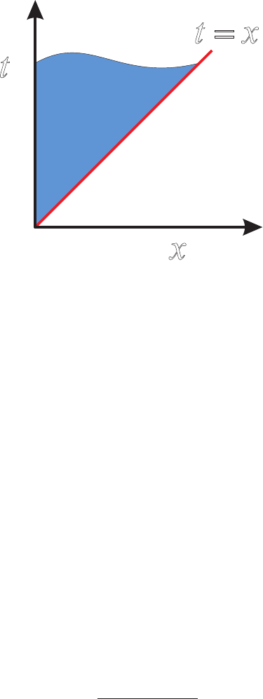
22 Solution 2.9
Figure 2 Plot of the region of integration of (62)
in (x, t)space.
t
x
t=x
2.9 When we integrate over µM−1the lower limit of integration is 0, while the upper
limit is 1−PM−2
j=1 µjsince the remaining probabilities must sum to one (see Fig-
ure 2.4). Thus we have
pM−1(µ1,...,µM−2) = Z1−PM−2
j=1 µj
0
pM(µ1,...,µM−1) dµM−1
=CM"M−2
Y
k=1
µαk−1
k#Z1−PM−2
j=1 µj
0
µαM−1−1
M−1 1−
M−1
X
j=1
µj!αM−1
dµM−1.
In order to make the limits of integration equal to 0and 1we change integration
variable from µM−1to tusing
µM−1=t 1−
M−2
X
j=1
µj!
which gives
pM−1(µ1, . . . , µM−2)
=CM"M−2
Y
k=1
µαk−1
k# 1−
M−2
X
j=1
µj!αM−1+αM−1Z1
0
tαM−1−1(1 −t)αM−1dt
=CM"M−2
Y
k=1
µαk−1
k# 1−
M−2
X
j=1
µj!αM−1+αM−1
Γ(αM−1)Γ(αM)
Γ(αM−1+αM)(65)
where we have used (2.265). The right hand side of (65) is seen to be a normalized
Dirichlet distribution over M−1variables, with coefficients α1,...,αM−2, αM−1+

Solution 2.11 23
αM, (note that we have effectively combined the final two categories) and we can
identify its normalization coefficient using (2.38). Thus
CM=Γ(α1+...+αM)
Γ(α1)...Γ(αM−2)Γ(αM−1+αM)·Γ(αM−1+αM)
Γ(αM−1)Γ(αM)
=Γ(α1+...+αM)
Γ(α1)...Γ(αM)(66)
as required.
2.11 We first of all write the Dirichlet distribution (2.38) in the form
Dir(µ|α) = K(α)
M
Y
k=1
µαk−1
k
where
K(α) = Γ(α0)
Γ(α1)···Γ(αM).
Next we note the following relation
∂
∂αj
M
Y
k=1
µαk−1
k=∂
∂αj
M
Y
k=1
exp ((αk−1) ln µk)
=
M
Y
k=1
ln µjexp {(αk−1) ln µk}
= ln µj
M
Y
k=1
µαk−1
k
from which we obtain
E[ln µj] = K(α)Z1
0···Z1
0
ln µj
M
Y
k=1
µαk−1
kdµ1... dµM
=K(α)∂
∂αjZ1
0···Z1
0
M
Y
k=1
µαk−1
kdµ1... dµM
=K(α)∂
∂µj
1
K(α)
=−∂
∂µj
ln K(α).
Finally, using the expression for K(α), together with the definition of the digamma
function ψ(·), we have
E[ln µj] = ψ(αj)−ψ(α0).

24 Solution 2.14
2.14 As for the univariate Gaussian considered in Section 1.6, we can make use of La-
grange multipliers to enforce the constraints on the maximum entropy solution. Note
that we need a single Lagrange multiplier for the normalization constraint (2.280),
aD-dimensional vector mof Lagrange multipliers for the Dconstraints given by
(2.281), and a D×Dmatrix Lof Lagrange multipliers to enforce the D2constraints
represented by (2.282). Thus we maximize
e
H[p] = −Zp(x) ln p(x) dx+λZp(x) dx−1
+mTZp(x)xdx−µ
+Tr LZp(x)(x−µ)(x−µ)Tdx−Σ.(67)
By functional differentiation (Appendix D) the maximum of this functional with
respect to p(x)occurs when
0 = −1−ln p(x) + λ+mTx+Tr{L(x−µ)(x−µ)T}.
Solving for p(x)we obtain
p(x) = exp λ−1 + mTx+ (x−µ)TL(x−µ).(68)
We now find the values of the Lagrange multipliers by applying the constraints. First
we complete the square inside the exponential, which becomes
λ−1 + x−µ+1
2L−1mT
Lx−µ+1
2L−1m+µTm−1
4mTL−1m.
We now make the change of variable
y=x−µ+1
2L−1m.
The constraint (2.281) then becomes
Zexp λ−1 + yTLy +µTm−1
4mTL−1my+µ−1
2L−1mdy=µ.
In the final parentheses, the term in yvanishes by symmetry, while the term in µ
simply integrates to µby virtue of the normalization constraint (2.280) which now
takes the form
Zexp λ−1 + yTLy +µTm−1
4mTL−1mdy= 1.
and hence we have
−1
2L−1m=0

Solution 2.16 25
where again we have made use of the constraint (2.280). Thus m=0and so the
density becomes
p(x) = exp λ−1 + (x−µ)TL(x−µ).
Substituting this into the final constraint (2.282), and making the change of variable
x−µ=zwe obtain
Zexp λ−1 + zTLzzzTdx=Σ.
Applying an analogous argument to that used to derive (2.64) we obtain L=−1
2Σ.
Finally, the value of λis simply that value needed to ensure that the Gaussian distri-
bution is correctly normalized, as derived in Section 2.3, and hence is given by
λ−1 = ln 1
(2π)D/2
1
|Σ|1/2.
2.16 We have p(x1) = N(x1|µ1, τ−1
1)and p(x2) = N(x2|µ2, τ−1
2). Since x=x1+x2
we also have p(x|x2) = N(x|µ1+x2, τ −1
1). We now evaluate the convolution
integral given by (2.284) which takes the form
p(x) = τ1
2π1/2τ2
2π1/2Z∞
−∞
exp n−τ1
2(x−µ1−x2)2−τ2
2(x2−µ2)2odx2.
(69)
Since the final result will be a Gaussian distribution for p(x)we need only evaluate
its precision, since, from (1.110), the entropy is determined by the variance or equiv-
alently the precision, and is independent of the mean. This allows us to simplify the
calculation by ignoring such things as normalization constants.
We begin by considering the terms in the exponent of (69) which depend on x2which
are given by
−1
2x2
2(τ1+τ2) + x2{τ1(x−µ1) + τ2µ2}
=−1
2(τ1+τ2)x2−τ1(x−µ1) + τ2µ2
τ1+τ22
+{τ1(x−µ1) + τ2µ2}2
2(τ1+τ2)
where we have completed the square over x2. When we integrate out x2, the first
term on the right hand side will simply give rise to a constant factor independent
of x. The second term, when expanded out, will involve a term in x2. Since the
precision of xis given directly in terms of the coefficient of x2in the exponent, it is
only such terms that we need to consider. There is one other term in x2arising from
the original exponent in (69). Combining these we have
−τ1
2x2+τ2
1
2(τ1+τ2)x2=−1
2
τ1τ2
τ1+τ2
x2

26 Solutions 2.17–2.20
from which we see that xhas precision τ1τ2/(τ1+τ2).
We can also obtain this result for the precision directly by appealing to the general
result (2.115) for the convolution of two linear-Gaussian distributions.
The entropy of xis then given, from (1.110), by
H[x] = 1
2ln 2π(τ1+τ2)
τ1τ2.
2.17 We can use an analogous argument to that used in the solution of Exercise 1.14.
Consider a general square matrix Λwith elements Λij . Then we can always write
Λ=ΛA+ΛSwhere
ΛS
ij =Λij + Λji
2,ΛA
ij =Λij −Λji
2(70)
and it is easily verified that ΛSis symmetric so that ΛS
ij = ΛS
ji, and ΛAis antisym-
metric so that ΛA
ij =−ΛS
ji. The quadratic form in the exponent of a D-dimensional
multivariate Gaussian distribution can be written
1
2
D
X
i=1
D
X
j=1
(xi−µi)Λij (xj−µj)(71)
where Λ=Σ−1is the precision matrix. When we substitute Λ=ΛA+ΛSinto
(71) we see that the term involving ΛAvanishes since for every positive term there
is an equal and opposite negative term. Thus we can always take Λto be symmetric.
2.20 Since u1, . . . , uDconstitute a basis for RD, we can write
a= ˆa1u1+ ˆa2u2+...+ ˆaDuD,
where ˆa1, . . . , ˆaDare coefficients obtained by projecting aon u1,...,uD. Note that
they typically do not equal the elements of a.
Using this we can write
aTΣa =ˆa1uT
1+...+ ˆaDuT
DΣ(ˆa1u1+...+ ˆaDuD)
and combining this result with (2.45) we get
ˆa1uT
1+...+ ˆaDuT
D(ˆa1λ1u1+...+ ˆaDλDuD).
Now, since uT
iuj= 1 only if i=j, and 0otherwise, this becomes
ˆa2
1λ1+...+ ˆa2
DλD
and since ais real, we see that this expression will be strictly positive for any non-
zero a, if all eigenvalues are strictly positive. It is also clear that if an eigenvalue,
λi, is zero or negative, there exist a vector a(e.g. a=ui), for which this expression
will be less than or equal to zero. Thus, that a matrix has eigenvectors which are all
strictly positive is a sufficient and necessary condition for the matrix to be positive
definite.
Solutions 2.22–2.28 27
2.22 Consider a matrix Mwhich is symmetric, so that MT=M. The inverse matrix
M−1satisfies
MM−1=I.
Taking the transpose of both sides of this equation, and using the relation (C.1), we
obtain M−1TMT=IT=I
since the identity matrix is symmetric. Making use of the symmetry condition for
Mwe then have M−1TM=I
and hence, from the definition of the matrix inverse,
M−1T=M−1
and so M−1is also a symmetric matrix.
2.24 Multiplying the left hand side of (2.76) by the matrix (2.287) trivially gives the iden-
tity matrix. On the right hand side consider the four blocks of the resulting parti-
tioned matrix:
upper left
AM −BD−1CM = (A−BD−1C)(A−BD−1C)−1=I
upper right
−AMBD−1+BD−1+BD−1CMBD−1
=−(A−BD−1C)(A−BD−1C)−1BD−1+BD−1
=−BD−1+BD−1=0
lower left
CM −DD−1CM =CM −CM =0
lower right
−CMBD−1+DD−1+DD−1CMBD−1=DD−1=I.
Thus the right hand side also equals the identity matrix.
2.28 For the marginal distribution p(x)we see from (2.92) that the mean is given by the
upper partition of (2.108) which is simply µ. Similarly from (2.93) we see that the
covariance is given by the top left partition of (2.105) and is therefore given by Λ−1.
Now consider the conditional distribution p(y|x). Applying the result (2.81) for the
conditional mean we obtain
µy|x=Aµ+b+AΛ−1Λ(x−µ) = Ax +b.

28 Solution 2.32
Similarly applying the result (2.82) for the covariance of the conditional distribution
we have
cov[y|x] = L−1+AΛ−1AT−AΛ−1ΛΛ−1AT=L−1
as required.
2.32 The quadratic form in the exponential of the joint distribution is given by
−1
2(x−µ)TΛ(x−µ)−1
2(y−Ax −b)TL(y−Ax −b).(72)
We now extract all of those terms involving xand assemble them into a standard
Gaussian quadratic form by completing the square
=−1
2xT(Λ+ATLA)x+xTΛµ+ATL(y−b)+ const
=−1
2(x−m)T(Λ+ATLA)(x−m)
+1
2mT(Λ+ATLA)m+ const (73)
where
m= (Λ+ATLA)−1Λµ+ATL(y−b).
We can now perform the integration over xwhich eliminates the first term in (73).
Then we extract the terms in yfrom the final term in (73) and combine these with
the remaining terms from the quadratic form (72) which depend on yto give
=−1
2yTL−LA(Λ+ATLA)−1ATLy
+yTL−LA(Λ+ATLA)−1ATLb
+LA(Λ+ATLA)−1Λµ.(74)
We can identify the precision of the marginal distribution p(y)from the second order
term in y. To find the corresponding covariance, we take the inverse of the precision
and apply the Woodbury inversion formula (2.289) to give
L−LA(Λ+ATLA)−1ATL−1=L−1+AΛ−1AT(75)
which corresponds to (2.110).
Next we identify the mean νof the marginal distribution. To do this we make use of
(75) in (74) and then complete the square to give
−1
2(y−ν)TL−1+AΛ−1AT−1(y−ν) + const
where
ν=L−1+AΛ−1AT(L−1+AΛ−1AT)−1b+LA(Λ+ATLA)−1Λµ.

Solution 2.34 29
Now consider the two terms in the square brackets, the first one involving band the
second involving µ. The first of these contribution simply gives b, while the term in
µcan be written
=L−1+AΛ−1ATLA(Λ+ATLA)−1Λµ
=A(I+Λ−1ATLA)(I+Λ−1ATLA)−1Λ−1Λµ=Aµ
where we have used the general result (BC)−1=C−1B−1. Hence we obtain
(2.109).
2.34 Differentiating (2.118) with respect to Σwe obtain two terms:
−N
2
∂
∂Σln |Σ| − 1
2
∂
∂Σ
N
X
n=1
(xn−µ)TΣ−1(xn−µ).
For the first term, we can apply (C.28) directly to get
−N
2
∂
∂Σln |Σ|=−N
2Σ−1T=−N
2Σ−1.
For the second term, we first re-write the sum
N
X
n=1
(xn−µ)TΣ−1(xn−µ) = NTr Σ−1S,
where
S=1
N
N
X
n=1
(xn−µ)(xn−µ)T.
Using this together with (C.21), in which x= Σij (element (i, j)in Σ), and proper-
ties of the trace we get
∂
∂Σij
N
X
n=1
(xn−µ)TΣ−1(xn−µ) = N∂
∂Σij
Tr Σ−1S
=NTr ∂
∂Σij
Σ−1S
=−NTr Σ−1∂Σ
∂Σij
Σ−1S
=−NTr ∂Σ
∂Σij
Σ−1SΣ−1
=−NΣ−1SΣ−1ij
where we have used (C.26). Note that in the last step we have ignored the fact that
Σij = Σji, so that ∂Σ/∂Σij has a 1in position (i, j)only and 0everywhere else.

30 Solution 2.36
Treating this result as valid nevertheless, we get
−1
2
∂
∂Σ
N
X
n=1
(xn−µ)TΣ−1(xn−µ) = N
2Σ−1SΣ−1.
Combining the derivatives of the two terms and setting the result to zero, we obtain
N
2Σ−1=N
2Σ−1SΣ−1.
Re-arrangement then yields
Σ=S
as required.
2.36 NOTE: In the 1st printing of PRML, there are mistakes that affect this solution. The
sign in (2.129) is incorrect, and this equation should read
θ(N)=θ(N−1) −aN−1z(θ(N−1)).
Then, in order to be consistent with the assumption that f(θ)>0for θ > θ?and
f(θ)<0for θ < θ?in Figure 2.10, we should find the root of the expected negative
log likelihood. This lead to sign changes in (2.133) and (2.134), but in (2.135), these
are cancelled against the change of sign in (2.129), so in effect, (2.135) remains
unchanged. Also, xnshould be xnon the l.h.s. of (2.133). Finally, the labels µand
µML in Figure 2.11 should be interchanged and there are corresponding changes to
the caption (see errata on the PRML web site for details).
Consider the expression for σ2
(N)and separate out the contribution from observation
xNto give
σ2
(N)=1
N
N
X
n=1
(xn−µ)2
=1
N
N−1
X
n=1
(xn−µ)2+(xN−µ)2
N
=N−1
Nσ2
(N−1) +(xN−µ)2
N
=σ2
(N−1) −1
Nσ2
(N−1) +(xN−µ)2
N
=σ2
(N−1) +1
N(xN−µ)2−σ2
(N−1).(76)
If we substitute the expression for a Gaussian distribution into the result (2.135) for

Solutions 2.40–2.46 31
the Robbins-Monro procedure applied to maximizing likelihood, we obtain
σ2
(N)=σ2
(N−1) +aN−1
∂
∂σ2
(N−1) (−1
2ln σ2
(N−1) −(xN−µ)2
2σ2
(N−1) )
=σ2
(N−1) +aN−1(−1
2σ2
(N−1)
+(xN−µ)2
2σ4
(N−1) )
=σ2
(N−1) +aN−1
2σ4
(N−1) (xN−µ)2−σ2
(N−1).(77)
Comparison of (77) with (76) allows us to identify
aN−1=2σ4
(N−1)
N.
2.40 The posterior distribution is proportional to the product of the prior and the likelihood
function
p(µ|X)∝p(µ)
N
Y
n=1
p(xn|µ,Σ).
Thus the posterior is proportional to an exponential of a quadratic form in µgiven
by
−1
2(µ−µ0)TΣ−1
0(µ−µ0)−1
2
N
X
n=1
(xn−µ)TΣ−1(xn−µ)
=−1
2µTΣ−1
0+NΣ−1µ+µT Σ−1
0µ0+Σ−1
N
X
n=1
xn!+ const
where ‘const.’ denotes terms independent of µ. Using the discussion following
(2.71) we see that the mean and covariance of the posterior distribution are given by
µN=Σ−1
0+NΣ−1−1Σ−1
0µ0+Σ−1NµML(78)
Σ−1
N=Σ−1
0+NΣ−1(79)
where µML is the maximum likelihood solution for the mean given by
µML =1
N
N
X
n=1
xn.
2.46 From (2.158), we have
Z∞
0
bae(−bτ)τa−1
Γ(a)τ
2π1/2
exp n−τ
2(x−µ)2odτ
=ba
Γ(a)1
2π1/2Z∞
0
τa−1/2exp −τb+(x−µ)2
2dτ.

32 Solution 2.47
We now make the proposed change of variable z=τ∆, where ∆ = b+ (x−µ)2/2,
yielding
ba
Γ(a)1
2π1/2
∆−a−1/2Z∞
0
za−1/2exp(−z) dz
=ba
Γ(a)1
2π1/2
∆−a−1/2Γ(a+ 1/2)
where we have used the definition of the Gamma function (1.141). Finally, we sub-
stitute b+ (x−µ)2/2for ∆,ν/2for aand ν/2λfor b:
Γ(−a+ 1/2)
Γ(a)ba1
2π1/2
∆a−1/2
=Γ ((ν+ 1)/2)
Γ(ν/2) ν
2λν/21
2π1/2ν
2λ+(x−µ)2
2−(ν+1)/2
=Γ ((ν+ 1)/2)
Γ(ν/2) ν
2λν/21
2π1/2ν
2λ−(ν+1)/21 + λ(x−µ)2
ν−(ν+1)/2
=Γ ((ν+ 1)/2)
Γ(ν/2) λ
νπ 1/21 + λ(x−µ)2
ν−(ν+1)/2
2.47 Ignoring the normalization constant, we write (2.159) as
St(x|µ, λ, ν)∝1 + λ(x−µ)2
ν−(ν−1)/2
= exp −ν−1
2ln 1 + λ(x−µ)2
ν.(80)
For large ν, we make use of the Taylor expansion for the logarithm in the form
ln(1 + ) = +O(2)(81)
to re-write (80) as
exp −ν−1
2ln 1 + λ(x−µ)2
ν
= exp −ν−1
2λ(x−µ)2
ν+O(ν−2)
= exp −λ(x−µ)2
2+O(ν−1).

Solutions 2.51–2.56 33
We see that in the limit ν→ ∞ this becomes, up to an overall constant, the same as
a Gaussian distribution with mean µand precision λ. Since the Student distribution
is normalized to unity for all values of νit follows that it must remain normalized in
this limit. The normalization coefficient is given by the standard expression (2.42)
for a univariate Gaussian.
2.51 Using the relation (2.296) we have
1 = exp(iA) exp(−iA) = (cos A+isin A)(cos A−isin A) = cos2A+ sin2A.
Similarly, we have
cos(A−B) = <exp{i(A−B)}
=<exp(iA) exp(−iB)
=<(cos A+isin A)(cos B−isin B)
= cos Acos B+ sin Asin B.
Finally
sin(A−B) = =exp{i(A−B)}
==exp(iA) exp(−iB)
==(cos A+isin A)(cos B−isin B)
= sin Acos B−cos Asin B.
2.56 We can most conveniently cast distributions into standard exponential family form by
taking the exponential of the logarithm of the distribution. For the Beta distribution
(2.13) we have
Beta(µ|a, b) = Γ(a+b)
Γ(a)Γ(b)exp {(a−1) ln µ+ (b−1) ln(1 −µ)}
which we can identify as being in standard exponential form (2.194) with
h(µ) = 1 (82)
g(a, b) = Γ(a+b)
Γ(a)Γ(b)(83)
u(µ) = ln µ
ln(1 −µ)(84)
η(a, b) = a−1
b−1.(85)
Applying the same approach to the gamma distribution (2.146) we obtain
Gam(λ|a, b) = ba
Γ(a)exp {(a−1) ln λ−bλ}.

34 Solution 2.60
from which it follows that
h(λ) = 1 (86)
g(a, b) = ba
Γ(a)(87)
u(λ) = λ
ln λ(88)
η(a, b) = −b
a−1.(89)
Finally, for the von Mises distribution (2.179) we make use of the identity (2.178) to
give
p(θ|θ0, m) = 1
2πI0(m)exp {mcos θcos θ0+msin θsin θ0}
from which we find
h(θ) = 1 (90)
g(θ0, m) = 1
2πI0(m)(91)
u(θ) = cos θ
sin θ(92)
η(θ0, m) = mcos θ0
msin θ0.(93)
2.60 The value of the density p(x)at a point xnis given by hj(n), where the notation j(n)
denotes that data point xnfalls within region j. Thus the log likelihood function
takes the form N
X
n=1
ln p(xn) =
N
X
n=1
ln hj(n).
We now need to take account of the constraint that p(x)must integrate to unity. Since
p(x)has the constant value hiover region i, which has volume ∆i, the normalization
constraint becomes Pihi∆i= 1. Introducing a Lagrange multiplier λwe then
minimize the function
N
X
n=1
ln hj(n)+λ X
i
hi∆i−1!
with respect to hkto give
0 = nk
hk
+λ∆k
where nkdenotes the total number of data points falling within region k. Multiplying
both sides by hk, summing over kand making use of the normalization constraint,

Solutions 3.1–3.4 35
we obtain λ=−N. Eliminating λthen gives our final result for the maximum
likelihood solution for hkin the form
hk=nk
N
1
∆k
.
Note that, for equal sized bins ∆k= ∆ we obtain a bin height hkwhich is propor-
tional to the fraction of points falling within that bin, as expected.
Chapter 3 Linear Models for Regression
3.1 NOTE: In the 1st printing of PRML, there is a 2missing in the denominator of the
argument to the ‘tanh’ function in equation (3.102).
Using (3.6), we have
2σ(2a)−1 = 2
1 + e−2a−1
=2
1 + e−2a−1 + e−2a
1 + e−2a
=1−e−2a
1 + e−2a
=ea−e−a
ea+e−a
= tanh(a)
If we now take aj= (x−µj)/2s, we can rewrite (3.101) as
y(x,w) = w0+
M
X
j=1
wjσ(2aj)
=w0+
M
X
j=1
wj
2(2σ(2aj)−1 + 1)
=u0+
M
X
j=1
ujtanh(aj),
where uj=wj/2, for j= 1,...,M, and u0=w0+PM
j=1 wj/2.

36 Solution 3.5
3.4 Let
eyn=w0+
D
X
i=1
wi(xni +ni)
=yn+
D
X
i=1
wini
where yn=y(xn,w)and ni ∼ N(0, σ2)and we have used (3.105). From (3.106)
we then define
e
E=1
2
N
X
n=1 {eyn−tn}2
=1
2
N
X
n=1 ey2
n−2eyntn+t2
n
=1
2
N
X
n=1
y2
n+ 2yn
D
X
i=1
wini + D
X
i=1
wini!2
−2tnyn−2tn
D
X
i=1
wini +t2
n
.
If we take the expectation of e
Eunder the distribution of ni, we see that the second
and fifth terms disappear, since E[ni] = 0, while for the third term we get
E
D
X
i=1
wini!2
=
D
X
i=1
w2
iσ2
since the ni are all independent with variance σ2.
From this and (3.106) we see that
Ehe
Ei=ED+1
2
D
X
i=1
w2
iσ2,
as required.
3.5 We can rewrite (3.30) as
1
2 M
X
j=1 |wj|q−η!60

Solutions 3.6–3.8 37
where we have incorporated the 1/2scaling factor for convenience. Clearly this does
not affect the constraint.
Employing the technique described in Appendix E, we can combine this with (3.12)
to obtain the Lagrangian function
L(w, λ) = 1
2
N
X
n=1{tn−wTφ(xn)}2+λ
2 M
X
j=1 |wj|q−η!
and by comparing this with (3.29) we see immediately that they are identical in their
dependence on w.
Now suppose we choose a specific value of λ > 0and minimize (3.29). Denoting
the resulting value of wby w?(λ), and using the KKT condition (E.11), we see that
the value of ηis given by
η=
M
X
j=1 |w?
j(λ)|q.
3.6 We first write down the log likelihood function which is given by
ln L(W,Σ) = −N
2ln |Σ| − 1
2
N
X
n=1
(tn−WTφ(xn))TΣ−1(tn−WTφ(xn)).
First of all we set the derivative with respect to Wequal to zero, giving
0 = −
N
X
n=1
Σ−1(tn−WTφ(xn))φ(xn)T.
Multiplying through by Σand introducing the design matrix Φand the target data
matrix Twe have
ΦTΦW =ΦTT
Solving for Wthen gives (3.15) as required.
The maximum likelihood solution for Σis easily found by appealing to the standard
result from Chapter 2 giving
Σ=1
N
N
X
n=1
(tn−WT
MLφ(xn))(tn−WT
MLφ(xn))T.
as required. Since we are finding a joint maximum with respect to both Wand Σ
we see that it is WML which appears in this expression, as in the standard result for
an unconditional Gaussian distribution.
3.8 Combining the prior
p(w) = N(w|mN,SN)

38 Solutions 3.10–3.15
and the likelihood
p(tN+1|xN+1,w) = β
2π1/2
exp −β
2(tN+1 −wTφN+1)2(94)
where φN+1 =φ(xN+1), we obtain a posterior of the form
p(w|tN+1,xN+1,mN,SN)
∝exp −1
2(w−mN)TS−1
N(w−mN)−1
2β(tN+1 −wTφN+1)2.
We can expand the argument of the exponential, omitting the −1/2factors, as fol-
lows
(w−mN)TS−1
N(w−mN) + β(tN+1 −wTφN+1)2
=wTS−1
Nw−2wTS−1
NmN
+βwTφT
N+1φN+1w−2βwTφN+1tN+1 + const
=wT(S−1
N+βφN+1φT
N+1)w−2wT(S−1
NmN+βφN+1tN+1) + const,
where const denotes remaining terms independent of w. From this we can read off
the desired result directly,
p(w|tN+1,xN+1,mN,SN) = N(w|mN+1,SN+1),
with
S−1
N+1 =S−1
N+βφN+1φT
N+1.(95)
and
mN+1 =SN+1(S−1
NmN+βφN+1tN+1).(96)
3.10 Using (3.3), (3.8) and (3.49), we can re-write (3.57) as
p(t|x,t, α, β) = ZN(t|φ(x)Tw, β−1)N(w|mN,SN) dw.
By matching the first factor of the integrand with (2.114) and the second factor with
(2.113), we obtain the desired result directly from (2.115).
3.15 This is easily shown by substituting the re-estimation formulae (3.92) and (3.95) into
(3.82), giving
E(mN) = β
2kt−ΦmNk2+α
2mT
NmN
=N−γ
2+γ
2=N
2.

Solutions 3.18–3.20 39
3.18 We can rewrite (3.79)
β
2kt−Φwk2+α
2wTw
=β
2tTt−2tTΦw +wTΦTΦw+α
2wTw
=1
2βtTt−2βtTΦw +wTAw
where, in the last line, we have used (3.81). We now use the tricks of adding 0=
mT
NAmN−mT
NAmNand using I=A−1A, combined with (3.84), as follows:
1
2βtTt−2βtTΦw +wTAw
=1
2βtTt−2βtTΦA−1Aw +wTAw
=1
2βtTt−2mT
NAw +wTAw +mT
NAmN−mT
NAmN
=1
2βtTt−mT
NAmN+1
2(w−mN)TA(w−mN).
Here the last term equals term the last term of (3.80) and so it remains to show that
the first term equals the r.h.s. of (3.82). To do this, we use the same tricks again:
1
2βtTt−mT
NAmN=1
2βtTt−2mT
NAmN+mT
NAmN
=1
2βtTt−2mT
NAA−1ΦTtβ+mT
NαI+βΦTΦmN
=1
2βtTt−2mT
NΦTtβ+βmT
NΦTΦmN+αmT
NmN
=1
2β(t−ΦmN)T(t−ΦmN) + αmT
NmN
=β
2kt−ΦmNk2+α
2mT
NmN
as required.
3.20 We only need to consider the terms of (3.86) that depend on α, which are the first,
third and fourth terms.
Following the sequence of steps in Section 3.5.2, we start with the last of these terms,
−1
2ln |A|.
From (3.81), (3.87) and the fact that that eigenvectors uiare orthonormal (see also
Appendix C), we find that the eigenvectors of Ato be α+λi. We can then use (C.47)
and the properties of the logarithm to take us from the left to the right side of (3.88).

40 Solution 3.23
The derivatives for the first and third term of (3.86) are more easily obtained using
standard derivatives and (3.82), yielding
1
2M
α+mT
NmN.
We combine these results into (3.89), from which we get (3.92) via (3.90). The
expression for γin (3.91) is obtained from (3.90) by substituting
M
X
i
λi+α
λi+α
for Mand re-arranging.
3.23 From (3.10), (3.112) and the properties of the Gaussian and Gamma distributions
(see Appendix B), we get
p(t) = ZZ p(t|w, β)p(w|β) dwp(β) dβ
=ZZ β
2πN/2
exp −β
2(t−Φw)T(t−Φw)
β
2πM/2
|S0|−1/2exp −β
2(w−m0)TS−1
0(w−m0)dw
Γ(a0)−1ba0
0βa0−1exp(−b0β) dβ
=ba0
0
((2π)M+N|S0|)1/2ZZ exp −β
2(t−Φw)T(t−Φw)
exp −β
2(w−m0)TS−1
0(w−m0)dw
βa0−1βN/2βM/2exp(−b0β) dβ
=ba0
0
((2π)M+N|S0|)1/2ZZ exp −β
2(w−mN)TS−1
N(w−mN)dw
exp −β
2tTt+mT
0S−1
0m0−mT
NS−1
NmN
βaN−1βM/2exp(−b0β) dβ

Solution 4.2 41
where we have completed the square for the quadratic form in w, using
mN=SNS−1
0m0+ΦTt
S−1
N=βS−1
0+ΦTΦ
aN=a0+N
2
bN=b0+1
2 mT
0S−1
0m0−mT
NS−1
NmN+
N
X
n=1
t2
n!.
Now we are ready to do the integration, first over wand then β, and re-arrange the
terms to obtain the desired result
p(t) = ba0
0
((2π)M+N|S0|)1/2(2π)M/2|SN|1/2ZβaN−1exp(−bNβ) dβ
=1
(2π)N/2|SN|1/2
|S0|1/2
ba0
0
baN
N
Γ(aN)
Γ(a0).
Chapter 4 Linear Models for Classification
4.2 For the purpose of this exercise, we make the contribution of the bias weights explicit
in (4.15), giving
ED(f
W) = 1
2Tr (XW +1wT
0−T)T(XW +1wT
0−T),(97)
where w0is the column vector of bias weights (the top row of f
Wtransposed) and 1
is a column vector of N ones.
We can take the derivative of (97) w.r.t. w0, giving
2Nw0+ 2(XW −T)T1.
Setting this to zero, and solving for w0, we obtain
w0=¯
t−WT¯
x(98)
where
¯
t=1
NTT1and ¯
x=1
NXT1.
If we subsitute (98) into (97), we get
ED(W) = 1
2Tr (XW +T−XW −T)T(XW +T−XW −T),

42 Solutions 4.4–4.7
where
T=1¯
tTand X=1¯
xT.
Setting the derivative of this w.r.t. Wto zero we get
W= ( b
XTb
X)−1b
XTb
T=b
X†b
T,
where we have defined b
X=X−Xand b
T=T−T.
Now consider the prediction for a new input vector x?,
y(x?) = WTx?+w0
=WTx?+¯
t−WT¯
x
=¯
t−b
TTb
X†T
(x?−¯
x).(99)
If we apply (4.157) to ¯
t, we get
aT¯
t=1
NaTTT1=−b.
Therefore, applying (4.157) to (99), we obtain
aTy(x?) = aT¯
t+aTb
TTb
X†T
(x?−¯
x)
=aT¯
t=−b,
since aTb
TT=aT(T−T)T=b(1−1)T=0T.
4.4 NOTE: In the 1st printing of PRML, the text of the exercise refers equation (4.23)
where it should refer to (4.22).
From (4.22) we can construct the Lagrangian function
L=wT(m2−m1) + λwTw−1.
Taking the gradient of Lwe obtain
∇L=m2−m1+ 2λw(100)
and setting this gradient to zero gives
w=−1
2λ(m2−m1)
form which it follows that w∝m2−m1.
4.7 From (4.59) we have
1−σ(a) = 1 −1
1 + e−a=1 + e−a−1
1 + e−a
=e−a
1 + e−a=1
ea+ 1 =σ(−a).

Solutions 4.9–4.12 43
The inverse of the logistic sigmoid is easily found as follows
y=σ(a) = 1
1 + e−a
⇒1
y−1 = e−a
⇒ln 1−y
y=−a
⇒ln y
1−y=a=σ−1(y).
4.9 The likelihood function is given by
p({φn,tn}|{πk}) =
N
Y
n=1
K
Y
k=1 {p(φn|Ck)πk}tnk
and taking the logarithm, we obtain
ln p({φn,tn}|{πk}) =
N
X
n=1
K
X
k=1
tnk {ln p(φn|Ck) + ln πk}.(101)
In order to maximize the log likelihood with respect to πkwe need to preserve the
constraint Pkπk= 1. This can be done by introducing a Lagrange multiplier λand
maximizing
ln p({φn,tn}|{πk}) + λ K
X
k=1
πk−1!.
Setting the derivative with respect to πkequal to zero, we obtain
N
X
n=1
tnk
πk
+λ= 0.
Re-arranging then gives
−πkλ=
N
X
n=1
tnk =Nk.(102)
Summing both sides over kwe find that λ=−N, and using this to eliminate λwe
obtain (4.159).

44 Solutions 4.13–4.17
4.12 Differentiating (4.59) we obtain
dσ
da =e−a
(1 + e−a)2
=σ(a)e−a
1 + e−a
=σ(a)1 + e−a
1 + e−a−1
1 + e−a
=σ(a)(1 −σ(a)).
4.13 We start by computing the derivative of (4.90) w.r.t. yn
∂E
∂yn
=1−tn
1−yn−tn
yn
(103)
=yn(1 −tn)−tn(1 −yn)
yn(1 −yn)
=yn−yntn−tn+yntn
yn(1 −yn)(104)
=yn−tn
yn(1 −yn).(105)
From (4.88), we see that
∂yn
∂an
=∂σ(an)
∂an
=σ(an) (1 −σ(an)) = yn(1 −yn).(106)
Finally, we have
∇an=φn(107)
where ∇denotes the gradient with respect to w. Combining (105), (106) and (107)
using the chain rule, we obtain
∇E=
N
X
n=1
∂E
∂yn
∂yn
∂an∇an
=
N
X
n=1
(yn−tn)φn
as required.
4.17 From (4.104) we have
∂yk
∂ak
=eak
Pieai−eak
Pieai2
=yk(1 −yk),
∂yk
∂aj
=−eakeaj
Pieai2=−ykyj, j 6=k.

Solutions 4.19–4.23 45
Combining these results we obtain (4.106).
4.19 Using the cross-entropy error function (4.90), and following Exercise 4.13, we have
∂E
∂yn
=yn−tn
yn(1 −yn).(108)
Also
∇an=φn.(109)
From (4.115) and (4.116) we have
∂yn
∂an
=∂Φ(an)
∂an
=1
√2πe−a2
n.(110)
Combining (108), (109) and (110), we get
∇E=
N
X
n=1
∂E
∂yn
∂yn
∂an∇an=
N
X
n=1
yn−tn
yn(1 −yn)
1
√2πe−a2
nφn.(111)
In order to find the expression for the Hessian, it is is convenient to first determine
∂
∂yn
yn−tn
yn(1 −yn)=yn(1 −yn)
y2
n(1 −yn)2−(yn−tn)(1 −2yn)
y2
n(1 −yn)2
=y2
n+tn−2yntn
y2
n(1 −yn)2.(112)
Then using (109)–(112) we have
∇∇E=
N
X
n=1 ∂
∂ynyn−tn
yn(1 −yn)1
√2πe−a2
nφn∇yn
+yn−tn
yn(1 −yn)
1
√2πe−a2
n(−2an)φn∇an
=
N
X
n=1 y2
n+tn−2yntn
yn(1 −yn)
1
√2πe−a2
n−2an(yn−tn)e−2a2
nφnφT
n
√2πyn(1 −yn).
4.23 NOTE: In the 1st printing of PRML, the text of the exercise contains a typographical
error. Following the equation, it should say that His the matrix of second derivatives
of the negative log likelihood.
The BIC approximation can be viewed as a large Napproximation to the log model
evidence. From (4.138), we have
A=−∇∇ln p(D|θMAP)p(θMAP)
=H− ∇∇ln p(θMAP)

46 Solution 5.2
and if p(θ) = N(θ|m,V0), this becomes
A=H+V−1
0.
If we assume that the prior is broad, or equivalently that the number of data points
is large, we can neglect the term V−1
0compared to H. Using this result, (4.137) can
be rewritten in the form
ln p(D)'ln p(D|θMAP)−1
2(θMAP −m)V−1
0(θMAP −m)−1
2ln |H|+ const
(113)
as required. Note that the phrasing of the question is misleading, since the assump-
tion of a broad prior, or of large N, is required in order to derive this form, as well
as in the subsequent simplification.
We now again invoke the broad prior assumption, allowing us to neglect the second
term on the right hand side of (113) relative to the first term.
Since we assume i.i.d. data, H=−∇∇ln p(D|θMAP)consists of a sum of terms,
one term for each datum, and we can consider the following approximation:
H=
N
X
n=1
Hn=Nb
H
where Hnis the contribution from the nth data point and
b
H=1
N
N
X
n=1
Hn.
Combining this with the properties of the determinant, we have
ln |H|= ln |Nb
H|= ln NM|b
H|=Mln N+ ln |b
H|
where Mis the dimensionality of θ. Note that we are assuming that b
Hhas full rank
M. Finally, using this result together (113), we obtain (4.139) by dropping the ln |b
H|
since this O(1) compared to ln N.
Chapter 5 Neural Networks
5.2 The likelihood function for an i.i.d. data set, {(x1,t1),...,(xN,tN)}, under the
conditional distribution (5.16) is given by
N
Y
n=1 Ntn|y(xn,w), β−1I.

Solutions 5.5–5.6 47
If we take the logarithm of this, using (2.43), we get
N
X
n=1
ln Ntn|y(xn,w), β−1I
=−1
2
N
X
n=1
(tn−y(xn,w))T(βI) (tn−y(xn,w)) + const
=−β
2
N
X
n=1 ktn−y(xn,w)k2+const,
where ‘const’ comprises terms which are independent of w. The first term on the
right hand side is proportional to the negative of (5.11) and hence maximizing the
log-likelihood is equivalent to minimizing the sum-of-squares error.
5.5 For the given interpretation of yk(x,w), the conditional distribution of the target
vector for a multiclass neural network is
p(t|w1,...,wK) =
K
Y
k=1
ytk
k.
Thus, for a data set of Npoints, the likelihood function will be
p(T|w1,...,wK) =
N
Y
n=1
K
Y
k=1
ytnk
nk .
Taking the negative logarithm in order to derive an error function we obtain (5.24)
as required. Note that this is the same result as for the multiclass logistic regression
model, given by (4.108) .
5.6 Differentiating (5.21) with respect to the activation ancorresponding to a particular
data point n, we obtain
∂E
∂an
=−tn
1
yn
∂yn
∂an
+ (1 −tn)1
1−yn
∂yn
∂an
.(114)
From (4.88), we have ∂yn
∂an
=yn(1 −yn).(115)
Substituting (115) into (114), we get
∂E
∂an
=−tn
yn(1 −yn)
yn
+ (1 −tn)yn(1 −yn)
(1 −yn)
=yn−tn
as required.

48 Solutions 5.9–5.10
5.9 This simply corresponds to a scaling and shifting of the binary outputs, which di-
rectly gives the activation function, using the notation from (5.19), in the form
y= 2σ(a)−1.
The corresponding error function can be constructed from (5.21) by applying the
inverse transform to ynand tn, yielding
E(w) = −
N
X
n=1
1 + tn
2ln 1 + yn
2+1−1 + tn
2ln 1−1 + yn
2
=−1
2
N
X
n=1 {(1 + tn) ln(1 + yn) + (1 −tn) ln(1 −yn)}+Nln 2
where the last term can be dropped, since it is independent of w.
To find the corresponding activation function we simply apply the linear transforma-
tion to the logistic sigmoid given by (5.19), which gives
y(a) = 2σ(a)−1 = 2
1 + e−a−1
=1−e−a
1 + e−a=ea/2−e−a/2
ea/2+e−a/2
= tanh(a/2).
5.10 From (5.33) and (5.35) we have
uT
iHui=uT
iλiui=λi.
Assume that His positive definite, so that (5.37) holds. Then by setting v=uiit
follows that
λi=uT
iHui>0(116)
for all values of i. Thus, if His positive definite, all of its eigenvalues will be
positive.
Conversely, assume that (116) holds. Then, for any vector, v, we can make use of
(5.38) to give
vTHv = X
i
ciui!T
H X
j
cjuj!
= X
i
ciui!T X
j
λjcjuj!
=X
i
λic2
i>0
where we have used (5.33) and (5.34) along with (116). Thus, if all of the eigenvalues
are positive, the Hessian matrix will be positive definite.

Solutions 5.11–5.19 49
5.11 NOTE: In PRML, Equation (5.32) contains a typographical error: =should be '.
We start by making the change of variable given by (5.35) which allows the error
function to be written in the form (5.36). Setting the value of the error function
E(w)to a constant value Cwe obtain
E(w?) + 1
2X
i
λiα2
i=C.
Re-arranging gives X
i
λiα2
i= 2C−2E(w?) = e
C
where e
Cis also a constant. This is the equation for an ellipse whose axes are aligned
with the coordinates described by the variables {αi}. The length of axis jis found
by setting αi= 0 for all i6=j, and solving for αjgiving
αj= e
C
λj!1/2
which is inversely proportional to the square root of the corresponding eigenvalue.
5.12 NOTE: See note in Solution 5.11.
From (5.37) we see that, if His positive definite, then the second term in (5.32) will
be positive whenever (w−w?)is non-zero. Thus the smallest value which E(w)
can take is E(w?), and so w?is the minimum of E(w).
Conversely, if w?is the minimum of E(w), then, for any vector w6=w?,E(w)>
E(w?). This will only be the case if the second term of (5.32) is positive for all
values of w6=w?(since the first term is independent of w). Since w−w?can be
set to any vector of real numbers, it follows from the definition (5.37) that Hmust
be positive definite.
5.19 If we take the gradient of (5.21) with respect to w, we obtain
∇E(w) =
N
X
n=1
∂E
∂an∇an=
N
X
n=1
(yn−tn)∇an,
where we have used the result proved earlier in the solution to Exercise 5.6. Taking
the second derivatives we have
∇∇E(w) =
N
X
n=1 ∂yn
∂an∇an∇an+ (yn−tn)∇∇an.
Dropping the last term and using the result (4.88) for the derivative of the logistic
sigmoid function, proved in the solution to Exercise 4.12, we finally get
∇∇E(w)'
N
X
n=1
yn(1 −yn)∇an∇an=
N
X
n=1
yn(1 −yn)bnbT
n
50 Solution 5.25
where bn≡ ∇an.
5.25 The gradient of (5.195) is given
∇E=H(w−w?)
and hence update formula (5.196) becomes
w(τ)=w(τ−1) −ρH(w(τ−1) −w?).
Pre-multiplying both sides with uT
jwe get
w(τ)
j=uT
jw(τ)(117)
=uT
jw(τ−1) −ρuT
jH(w(τ−1) −w?)
=w(τ−1)
j−ρηjuT
j(w−w?)
=w(τ−1)
j−ρηj(w(τ−1)
j−w?
j),(118)
where we have used (5.198). To show that
w(τ)
j={1−(1 −ρηj)τ}w?
j
for τ= 1,2,..., we can use proof by induction. For τ= 1, we recall that w(0) =0
and insert this into (118), giving
w(1)
j=w(0)
j−ρηj(w(0)
j−w?
j)
=ρηjw?
j
={1−(1 −ρηj)}w?
j.
Now we assume that the result holds for τ=N−1and then make use of (118)
w(N)
j=w(N−1)
j−ρηj(w(N−1)
j−w?
j)
=w(N−1)
j(1 −ρηj) + ρηjw?
j
=1−(1 −ρηj)N−1w?
j(1 −ρηj) + ρηjw?
j
=(1 −ρηj)−(1 −ρηj)Nw?
j+ρηjw?
j
=1−(1 −ρηj)Nw?
j
as required.
Provided that |1−ρηj|<1then we have (1 −ρηj)τ→0as τ→ ∞, and hence
1−(1 −ρηj)N→1and w(τ)→w?.
If τis finite but ηj(ρτ)−1,τmust still be large, since ηjρτ 1, even though
|1−ρηj|<1. If τis large, it follows from the argument above that w(τ)
j'w?
j.

Solution 5.27 51
If, on the other hand, ηj(ρτ )−1, this means that ρηjmust be small, since ρηjτ
1and τis an integer greater than or equal to one. If we expand,
(1 −ρηj)τ= 1 −τρηj+O(ρη2
j)
and insert this into (5.197), we get
|w(τ)
j|=|{1−(1 −ρηj)τ}w?
j|
=|1−(1 −τρηj+O(ρη2
j))w?
j|
'τρηj|w?
j| |w?
j|
Recall that in Section 3.5.3 we showed that when the regularization parameter (called
αin that section) is much larger than one of the eigenvalues (called λjin that section)
then the corresponding parameter value wiwill be close to zero. Conversely, when
αis much smaller than λithen wiwill be close to its maximum likelihood value.
Thus αis playing an analogous role to ρτ.
5.27 If s(x,ξ) = x+ξ, then
∂sk
∂ξi
=Iki, i.e., ∂s
∂ξ=I,
and since the first order derivative is constant, there are no higher order derivatives.
We now make use of this result to obtain the derivatives of yw.r.t. ξi:
∂y
∂ξi
=X
k
∂y
∂sk
∂sk
∂ξi
=∂y
∂si
=bi
∂y
∂ξi∂ξj
=∂bi
∂ξj
=X
k
∂bi
∂sk
∂sk
∂ξj
=∂bi
∂sj
=Bij
Using these results, we can write the expansion of e
Eas follows:
e
E=1
2ZZZ{y(x)−t}2p(t|x)p(x)p(ξ) dξdxdt
+ZZZ{y(x)−t}bTξp(ξ)p(t|x)p(x) dξdxdt
+1
2ZZZ ξT{y(x)−t}B+bbTξp(ξ)p(t|x)p(x) dξdxdt.
The middle term will again disappear, since E[ξ] = 0and thus we can write e
Eon
the form of (5.131) with
Ω = 1
2ZZZ ξT{y(x)−t}B+bbTξp(ξ)p(t|x)p(x) dξdxdt.

52 Solutions 5.28–5.34
Again the first term within the parenthesis vanishes to leading order in ξand we are
left with
Ω'1
2ZZ ξTbbTξp(ξ)p(x) dξdx
=1
2ZZ Trace ξξTbbTp(ξ)p(x) dξdx
=1
2ZTrace IbbTp(x) dx
=1
2ZbTbp(x) dx=1
2Zk∇y(x)k2p(x) dx,
where we used the fact that E[ξξT] = I.
5.28 The modifications only affect derivatives with respect to weights in the convolutional
layer. The units within a feature map (indexed m) have different inputs, but all share
a common weight vector, w(m). Thus, errors δ(m)from all units within a feature
map will contribute to the derivatives of the corresponding weight vector. In this
situation, (5.50) becomes
∂En
∂w(m)
i
=X
j
∂En
∂a(m)
j
∂a(m)
j
∂w(m)
i
=X
j
δ(m)
jz(m)
ji .
Here a(m)
jdenotes the activation of the jth unit in the mth feature map, whereas
w(m)
idenotes the ith element of the corresponding feature vector and, finally, z(m)
ji
denotes the ith input for the jth unit in the mth feature map; the latter may be an
actual input or the output of a preceding layer.
Note that δ(m)
j=∂En/∂a(m)
jwill typically be computed recursively from the δs
of the units in the following layer, using (5.55). If there are layer(s) preceding the
convolutional layer, the standard backward propagation equations will apply; the
weights in the convolutional layer can be treated as if they were independent param-
eters, for the purpose of computing the δs for the preceding layer’s units.
5.29 This is easily verified by taking the derivative of (5.138), using (1.46) and standard
derivatives, yielding
∂Ω
∂wi
=1
PkπkN(wi|µk, σ2
k)X
j
πjN(wi|µj, σ2
j)(wi−µj)
σ2.
Combining this with (5.139) and (5.140), we immediately obtain the second term of
(5.141).
5.34 NOTE: In the 1st printing of PRML, the l.h.s. of (5.154) should be replaced with
γnk =γk(tn|xn). Accordingly, in (5.155) and (5.156), γkshould be replaced by
γnk and in (5.156), tlshould be tnl.

Solution 5.39 53
We start by using the chain rule to write
∂En
∂aπ
k
=
K
X
j=1
∂En
∂πj
∂πj
∂aπ
k
.(119)
Note that because of the coupling between outputs caused by the softmax activation
function, the dependence on the activation of a single output unit involves all the
output units.
For the first factor inside the sum on the r.h.s. of (119), standard derivatives applied
to the nth term of (5.153) gives
∂En
∂πj
=−Nnj
PK
l=1 πlNnl
=−γnj
πj
.(120)
For the for the second factor, we have from (4.106) that
∂πj
∂aπ
k
=πj(Ijk −πk).(121)
Combining (119), (120) and (121), we get
∂En
∂aπ
k
=−
K
X
j=1
γnj
πj
πj(Ijk −πk)
=−
K
X
j=1
γnj (Ijk −πk) = −γnk +
K
X
j=1
γnjπk=πk−γnk,
where we have used the fact that, by (5.154), PK
j=1 γnj = 1 for all n.
5.39 Using (4.135), we can approximate (5.174) as
p(D|α, β)'p(D|wMAP, β)p(wMAP|α)
Zexp −1
2(w−wMAP)TA(w−wMAP)dw,
where Ais given by (5.166), as p(D|w, β)p(w|α)is proportional to p(w|D, α, β).
Using (4.135), (5.162) and (5.163), we can rewrite this as
p(D|α, β)'
N
Y
nN(tn|y(xn,wMAP), β−1)N(wMAP|0, α−1I)(2π)W/2
|A|1/2.
Taking the logarithm of both sides and then using (2.42) and (2.43), we obtain the
desired result.

54 Solutions 5.40–6.1
5.40 For a K-class neural network, the likelihood function is given by
N
Y
n
K
Y
k
yk(xn,w)tnk
and the corresponding error function is given by (5.24).
Again we would use a Laplace approximation for the posterior distribution over the
weights, but the corresponding Hessian matrix, H, in (5.166), would now be derived
from (5.24). Similarly, (5.24), would replace the binary cross entropy error term in
the regularized error function (5.184).
The predictive distribution for a new pattern would again have to be approximated,
since the resulting marginalization cannot be done analytically. However, in con-
trast to the two-class problem, there is no obvious candidate for this approximation,
although Gibbs (1997) discusses various alternatives.
Chapter 6 Kernel Methods
6.1 We first of all note that J(a)depends on aonly through the form Ka. Since typically
the number Nof data points is greater than the number Mof basis functions, the
matrix K=ΦΦTwill be rank deficient. There will then be Meigenvectors of K
having non-zero eigenvalues, and N−Meigenvectors with eigenvalue zero. We can
then decompose a=a+a⊥where aT
a⊥= 0 and Ka⊥=0. Thus the value of
a⊥is not determined by J(a). We can remove the ambiguity by setting a⊥=0, or
equivalently by adding a regularizer term
2aT
⊥a⊥
to J(a)where is a small positive constant. Then a=awhere alies in the span
of K=ΦΦTand hence can be written as a linear combination of the columns of
Φ, so that in component notation
an=
M
X
i=1
uiφi(xn)
or equivalently in vector notation
a=Φu.(122)
Substituting (122) into (6.7) we obtain
J(u) = 1
2(KΦu −t)T(KΦu −t) + λ
2uTΦTKΦu
=1
2ΦΦTΦu −tTΦΦTΦu −t+λ
2uTΦTΦΦTΦu (123)
Solutions 6.5–6.7 55
Since the matrix ΦTΦhas full rank we can define an equivalent parametrization
given by
w=ΦTΦu
and substituting this into (123) we recover the original regularized error function
(6.2).
6.5 The results (6.13) and (6.14) are easily proved by using (6.1) which defines the kernel
in terms of the scalar product between the feature vectors for two input vectors. If
k1(x,x)is a valid kernel then there must exist a feature vector φ(x)such that
k1(x,x) = φ(x)Tφ(x).
It follows that
ck1(x,x) = u(x)Tu(x)
where
u(x) = c1/2φ(x)
and so ck1(x,x)can be expressed as the scalar product of feature vectors, and hence
is a valid kernel.
Similarly, for (6.14) we can write
f(x)k1(x,x)f(x) = v(x)Tv(x)
where we have defined
v(x) = f(x)φ(x).
Again, we see that f(x)k1(x,x)f(x)can be expressed as the scalar product of
feature vectors, and hence is a valid kernel.
Alternatively, these results can be proved be appealing to the general result that
the Gram matrix, K, whose elements are given by k(xn,xm), should be positive
semidefinite for all possible choices of the set {xn}, by following a similar argu-
ment to Solution 6.7 below.
6.7 (6.17) is most easily proved by making use of the result, discussed on page 295, that
a necessary and sufficient condition for a function k(x,x)to be a valid kernel is
that the Gram matrix K, whose elements are given by k(xn,xm), should be positive
semidefinite for all possible choices of the set {xn}. A matrix Kis positive semi-
definite if, and only if,
aTKa >0
for any choice of the vector a. Let K1be the Gram matrix for k1(x,x)and let K2
be the Gram matrix for k2(x,x). Then
aT(K1+K2)a=aTK1a+aTK2a>0
where we have used the fact that K1and K2are positive semi-definite matrices,
together with the fact that the sum of two non-negative numbers will itself be non-
negative. Thus, (6.17) defines a valid kernel.
56 Solutions 6.12–6.14
To prove (6.18), we take the approach adopted in Solution 6.5. Since we know that
k1(x,x)and k2(x,x)are valid kernels, we know that there exist mappings φ(x)
and ψ(x)such that
k1(x,x) = φ(x)Tφ(x)and k2(x,x) = ψ(x)Tψ(x).
Hence
k(x,x) = k1(x,x)k2(x,x)
=φ(x)Tφ(x)ψ(x)Tψ(x)
=
M
X
m=1
φm(x)φm(x)
N
X
n=1
ψn(x)ψn(x)
=
M
X
m=1
N
X
n=1
φm(x)φm(x)ψn(x)ψn(x)
=
K
X
k=1
ϕk(x)ϕk(x)
=ϕ(x)Tϕ(x),
where K=MN and
ϕk(x) = φ((k−1)N)+1(x)ψ((k−1)N)+1(x),
where in turn and denote integer division and remainder, respectively.
6.12 NOTE: In the 1st printing of PRML, there is an error in the text relating to this
exercise. Immediately following (6.27), it says: |A|denotes the number of subsets
in A; it should have said: |A|denotes the number of elements in A.
Since Amay be equal to D(the subset relation was not defined to be strict), φ(D)
must be defined. This will map to a vector of 2|D|1s, one for each possible subset
of D, including Ditself as well as the empty set. For A⊂D,φ(A)will have 1s in
all positions that correspond to subsets of Aand 0s in all other positions. Therefore,
φ(A1)Tφ(A2)will count the number of subsets shared by A1and A2. However, this
can just as well be obtained by counting the number of elements in the intersection
of A1and A2, and then raising 2 to this number, which is exactly what (6.27) does.
6.14 In order to evaluate the Fisher kernel for the Gaussian we first note that the covari-
ance is assumed to be fixed, and hence the parameters comprise only the elements of
the mean µ. The first step is to evaluate the Fisher score defined by (6.32). From the
definition (2.43) of the Gaussian we have
g(µ,x) = ∇µln N(x|µ,S) = S−1(x−µ).
Next we evaluate the Fisher information matrix using the definition (6.34), giving
F=Exg(µ,x)g(µ,x)T=S−1Ex(x−µ)(x−µ)TS−1.

Solution 6.17 57
Here the expectation is with respect to the original Gaussian distribution, and so we
can use the standard result
Ex(x−µ)(x−µ)T=S
from which we obtain
F=S−1.
Thus the Fisher kernel is given by
k(x,x) = (x−µ)TS−1(x−µ),
which we note is just the squared Mahalanobis distance.
6.17 NOTE: In the 1st printing of PRML, there are typographical errors in the text relating
to this exercise. In the sentence following immediately after (6.39), f(x)should be
replaced by y(x). Also, on the l.h.s. of (6.40), y(xn)should be replaced by y(x).
There were also errors in Appendix D, which might cause confusion; please consult
the errata on the PRML website.
Following the discussion in Appendix D we give a first-principles derivation of the
solution. First consider a variation in the function y(x)of the form
y(x)→y(x) + η(x).
Substituting into (6.39) we obtain
E[y+η] = 1
2
N
X
n=1 Z{y(xn+ξ) + η(xn+ξ)−tn}2ν(ξ) dξ.
Now we expand in powers of and set the coefficient of , which corresponds to the
functional first derivative, equal to zero, giving
N
X
n=1 Z{y(xn+ξ)−tn}η(xn+ξ)ν(ξ) dξ= 0.(124)
This must hold for every choice of the variation function η(x). Thus we can choose
η(x) = δ(x−z)
where δ(·)is the Dirac delta function. This allows us to evaluate the integral over ξ
giving
N
X
n=1 Z{y(xn+ξ)−tn}δ(xn+ξ−z)ν(ξ) dξ=
N
X
n=1 {y(z)−tn}ν(z−xn).
Substituting this back into (124) and rearranging we then obtain the required result
(6.40).

58 Solutions 6.20–6.21
6.20 Given the joint distribution (6.64), we can identify tN+1 with xaand twith xbin
(2.65). Note that this means that we are prepending rather than appending tN+1 to t
and CN+1 therefore gets redefined as
CN+1 =ckT
k CN.
It then follows that
µa= 0 µb=0 xb=t
Σaa =cΣbb =CNΣab =ΣT
ba =kT
in (2.81) and (2.82), from which (6.66) and (6.67) follows directly.
6.21 Both the Gaussian process and the linear regression model give rise to Gaussian
predictive distributions p(tN+1|xN+1)so we simply need to show that these have
the same mean and variance. To do this we make use of the expression (6.54) for the
kernel function defined in terms of the basis functions. Using (6.62) the covariance
matrix CNthen takes the form
CN=1
αΦΦT+β−1IN(125)
where Φis the design matrix with elements Φnk =φk(xn), and INdenotes the
N×Nunit matrix. Consider first the mean of the Gaussian process predictive
distribution, which from (125), (6.54), (6.66) and the definitions in the text preceding
(6.66) is given by
mN+1 =α−1φ(xN+1)TΦTα−1ΦΦT+β−1IN−1t.
We now make use of the matrix identity (C.6) to give
ΦTα−1ΦΦT+β−1IN−1=αβ βΦTΦ+αIM−1ΦT=αβSNΦT.
Thus the mean becomes
mN+1 =βφ(xN+1)TSNΦTt
which we recognize as the mean of the predictive distribution for the linear regression
model given by (3.58) with mNdefined by (3.53) and SNdefined by (3.54).
For the variance we similarly substitute the expression (125) for the kernel func-
tion into the Gaussian process variance given by (6.67) and then use (6.54) and the
definitions in the text preceding (6.66) to obtain
σ2
N+1(xN+1) = α−1φ(xN+1)Tφ(xN+1) + β−1
−α−2φ(xN+1)TΦTα−1ΦΦT+β−1IN−1Φφ(xN+1)
=β−1+φ(xN+1)Tα−1IM
−α−2ΦTα−1ΦΦT+β−1IN−1Φφ(xN+1).(126)

Solutions 6.23–7.1 59
We now make use of the matrix identity (C.7) to give
α−1IM−α−1IMΦTΦ(α−1IM)ΦT+β−1IN−1Φα−1IM
=αI+βΦTΦ−1=SN,
where we have also used (3.54). Substituting this in (126), we obtain
σ2
N(xN+1) = 1
β+φ(xN+1)TSNφ(xN+1)
as derived for the linear regression model in Section 3.3.2.
6.23 NOTE: In the 1st printing of PRML, a typographical mistake appears in the text
of the exercise at line three, where it should say “... a training set of input vectors
x1,...,xN”.
If we assume that the target variables, t1,...,tD, are independent given the input
vector, x, this extension is straightforward.
Using analogous notation to the univariate case,
p(tN+1|T) = N(tN+1|m(xN+1), σ(xN+1)I),
where Tis a N×Dmatrix with the vectors tT
1,...,tT
Nas its rows,
m(xN+1)T=kTCNT
and σ(xN+1)is given by (6.67). Note that CN, which only depend on the input
vectors, is the same in the uni- and multivariate models.
6.25 Substituting the gradient and the Hessian into the Newton-Raphson formula we ob-
tain
anew
N=aN+ (C−1
N+WN)−1tN−σN−C−1
NaN
= (C−1
N+WN)−1[tN−σN+WNaN]
=CN(I+WNCN)−1[tN−σN+WNaN]
Chapter 7 Sparse Kernel Machines
7.1 From Bayes’ theorem we have
p(t|x)∝p(x|t)p(t)
where, from (2.249),
p(x|t) = 1
Nt
N
X
n=1
1
Zk
k(x,xn)δ(t, tn).

60 Solution 7.4
Here Ntis the number of input vectors with label t(+1 or −1) and N=N+1 +N−1.
δ(t, tn)equals 1if t=tnand 0otherwise. Zkis the normalisation constant for
the kernel. The minimum misclassification-rate is achieved if, for each new input
vector, ˜
x, we chose ˜
tto maximise p(˜
t|˜
x). With equal class priors, this is equivalent
to maximizing p(˜
x|˜
t)and thus
˜
t=
+1 iff 1
N+1 X
i:ti=+1
k(˜
x,xi)>1
N−1X
j:tj=−1
k(˜
x,xj)
−1otherwise.
Here we have dropped the factor 1/Zksince it only acts as a common scaling factor.
Using the encoding scheme for the label, this classification rule can be written in the
more compact form
˜
t= sign N
X
n=1
tn
Ntn
k(˜
x,xn)!.
Now we take k(x,xn) = xTxn, which results in the kernel density
p(x|t= +1) = 1
N+1 X
n:tn=+1
xTxn=xT¯
x+.
Here, the sum in the middle experssion runs over all vectors xnfor which tn= +1
and ¯
x+denotes the mean of these vectors, with the corresponding definition for the
negative class. Note that this density is improper, since it cannot be normalized.
However, we can still compare likelihoods under this density, resulting in the classi-
fication rule
˜
t=+1 if ˜
xT¯
x+>˜
xT¯
x−,
−1otherwise.
The same argument would of course also apply in the feature space φ(x).
7.4 From Figure 4.1 and (7.4), we see that the value of the margin
ρ=1
kwkand so 1
ρ2=kwk2.
From (7.16) we see that, for the maximum margin solution, the second term of (7.7)
vanishes and so we have
L(w, b, a) = 1
2kwk2.
Using this together with (7.8), the dual (7.10) can be written as
1
2kwk2=
N
X
n
an−1
2kwk2,
from which the desired result follows.

Solutions 7.8–7.10 61
7.8 This follows from (7.67) and (7.68), which in turn follow from the KKT conditions,
(E.9)–(E.11), for µn,ξn,bµnand b
ξn, and the results obtained in (7.59) and (7.60).
For example, for µnand ξn, the KKT conditions are
ξn>0
µn>0
µnξn= 0 (127)
and from (7.59) we have that
µn=C−an.(128)
Combining (127) and (128), we get (7.67); similar reasoning for bµnand b
ξnlead to
(7.68).
7.10 We first note that this result is given immediately from (2.113)–(2.115), but the task
set in the exercise was to practice the technique of completing the square. In this
solution and that of Exercise 7.12, we broadly follow the presentation in Section
3.5.1. Using (7.79) and (7.80), we can write (7.84) in a form similar to (3.78)
p(t|X,α, β) = β
2πN/21
(2π)N/2
M
Y
i=1
αiZexp {−E(w)}dw(129)
where
E(w) = β
2kt−Φwk2+1
2wTAw
and A= diag(α).
Completing the square over w, we get
E(w) = 1
2(w−m)TΣ−1(w−m) + E(t)(130)
where mand Σare given by (7.82) and (7.83), respectively, and
E(t) = 1
2βtTt−mTΣ−1m.(131)
Using (130), we can evaluate the integral in (129) to obtain
Zexp {−E(w)}dw= exp {−E(t)}(2π)M/2|Σ|1/2.(132)
Considering this as a function of twe see from (7.83), that we only need to deal
with the factor exp {−E(t)}. Using (7.82), (7.83), (C.7) and (7.86), we can re-write

62 Solution 7.12
(131) as follows
E(t) = 1
2βtTt−mTΣ−1m
=1
2βtTt−βtTΦΣΣ−1ΣΦTtβ
=1
2tTβI−βΦΣΦTβt
=1
2tTβI−βΦ(A+βΦTΦ)−1ΦTβt
=1
2tTβ−1I+ΦA−1ΦT−1t
=1
2tTC−1t.
This gives us the last term on the r.h.s. of (7.85); the two preceding terms are given
implicitly, as they form the normalization constant for the posterior Gaussian distri-
bution p(t|X,α, β).
7.12 Using the results (129)–(132) from Solution 7.10, we can write (7.85) in the form of
(3.86):
ln p(t|X,α, β) = N
2ln β+1
2
N
X
i
ln αi−E(t)−1
2ln |Σ| − N
2ln(2π).(133)
By making use of (131) and (7.83) together with (C.22), we can take the derivatives
of this w.r.t αi, yielding
∂
∂αi
ln p(t|X,α, β) = 1
2αi−1
2Σii −1
2m2
i.(134)
Setting this to zero and re-arranging, we obtain
αi=1−αiΣii
m2
i
=γi
m2
i
,
where we have used (7.89). Similarly, for βwe see that
∂
∂β ln p(t|X,α, β) = 1
2N
β− kt−Φmk2−Tr ΣΦTΦ.(135)
Using (7.83), we can rewrite the argument of the trace operator as
ΣΦTΦ=ΣΦTΦ+β−1ΣA −β−1ΣA
=Σ(ΦTΦβ+A)β−1−β−1ΣA
= (A+βΦTΦ)−1(ΦTΦβ+A)β−1−β−1ΣA
= (I−AΣ)β−1.(136)
Here the first factor on the r.h.s. of the last line equals (7.89) written in matrix form.
We can use this to set (135) equal to zero and then re-arrange to obtain (7.88).

Solutions 7.15–8.1 63
7.15 Using (7.94), (7.95) and (7.97)–(7.99), we can rewrite (7.85) as follows
ln p(t|X,α, β) = −1
2Nln(2π) + ln |C−i||1 + α−1
iϕT
iC−1
−iϕi|
+tTC−1
−i−C−1
−iϕiϕT
iC−1
−i
αi+ϕT
iC−1
−iϕit
=−1
2Nln(2π) + ln |C−i|+tTC−1
−it
+1
2−ln |1 + α−1
iϕT
iC−1
−iϕi|+tTC−1
−iϕiϕT
iC−1
−i
αi+ϕT
iC−1
−iϕi
t
=L(α−i) + 1
2ln αi−ln(αi+si) + q2
i
αi+si
=L(α−i) + λ(αi)
7.18 As the RVM can be regarded as a regularized logistic regression model, we can
follow the sequence of steps used to derive (4.91) in Exercise 4.13 to derive the first
term of the r.h.s. of (7.110), whereas the second term follows from standard matrix
derivatives (see Appendix C). Note however, that in Exercise 4.13 we are dealing
with the negative log-likelhood.
To derive (7.111), we make use of (106) and (107) from Exercise 4.13. If we write
the first term of the r.h.s. of (7.110) in component form we get
∂
∂wj
N
X
n=1
(tn−yn)φni =−
N
X
n=1
∂yn
∂an
∂an
∂wj
φni
=−
N
X
n=1
yn(1 −yn)φnjφni,
which, written in matrix form, equals the first term inside the parenthesis on the r.h.s.
of (7.111). The second term again follows from standard matrix derivatives.
Chapter 8 Graphical Models
8.1 We want to show that, for (8.5),
X
x1
...X
xK
p(x) = X
x1
...X
xK
K
Y
k=1
p(xk|pak) = 1.
We assume that the nodes in the graph has been numbered such that x1is the root
node and no arrows lead from a higher numbered node to a lower numbered node.
64 Solutions 8.2–8.9
We can then marginalize over the nodes in reverse order, starting with xK
X
x1
...X
xK
p(x) = X
x1
...X
xK
p(xK|paK)
K−1
Y
k=1
p(xk|pak)
=X
x1
... X
xK−1
K−1
Y
k=1
p(xk|pak),
since each of the conditional distributions is assumed to be correctly normalized and
none of the other variables depend on xK. Repeating this process K−2times we
are left with X
x1
p(x1|∅) = 1.
8.2 Consider a directed graph in which the nodes of the graph are numbered such that
are no edges going from a node to a lower numbered node. If there exists a directed
cycle in the graph then the subset of nodes belonging to this directed cycle must also
satisfy the same numbering property. If we traverse the cycle in the direction of the
edges the node numbers cannot be monotonically increasing since we must end up
back at the starting node. It follows that the cycle cannot be a directed cycle.
8.5 NOTE: In PRML, Equation (7.79) contains a typographical error: p(tn|xn,w, β−1)
should be p(tn|xn,w, β). This correction is provided for completeness only; it does
not affect this solution.
The solution is given in Figure 3.
Figure 3 The graphical representation of the relevance
vector machine (RVM); Solution 8.5.
tn
xn
N
wi
β
αi
M
8.8 a⊥⊥ b, c |dcan be written as
p(a, b, c|d) = p(a|d)p(b, c|d).
Summing (or integrating) both sides with respect to c, we obtain
p(a, b|d) = p(a|d)p(b|d)or a⊥⊥ b|d,
as desired.
8.9 Consider Figure 8.26. In order to apply the d-separation criterion we need to con-
sider all possible paths from the central node xito all possible nodes external to the
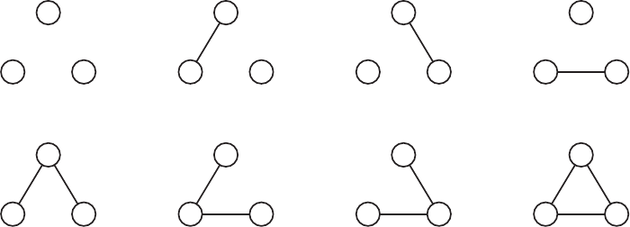
Solutions 8.12–8.15 65
Markov blanket. There are three possible categories of such paths. First, consider
paths via the parent nodes. Since the link from the parent node to the node xihas its
tail connected to the parent node, it follows that for any such path the parent node
must be either tail-to-tail or head-to-tail with respect to the path. Thus the observa-
tion of the parent node will block any such path. Second consider paths via one of
the child nodes of node xiwhich do not pass directly through any of the co-parents.
By definition such paths must pass to a child of the child node and hence will be
head-to-tail with respect to the child node and so will be blocked. The third and
final category of path passes via a child node of xiand then a co-parent node. This
path will be head-to-head with respect to the observed child node and hence will
not be blocked by the observed child node. However, this path will either tail-to-
tail or head-to-tail with respect to the co-parent node and hence observation of the
co-parent will block this path. We therefore see that all possible paths leaving node
xiwill be blocked and so the distribution of xi, conditioned on the variables in the
Markov blanket, will be independent of all of the remaining variables in the graph.
8.12 In an undirected graph of Mnodes there could potentially be a link between each
pair of nodes. The number of distinct graphs is then 2 raised to the power of the
number of potential links. To evaluate the number of distinct links, note that there
are Mnodes each of which could have a link to any of the other M−1nodes,
making a total of M(M−1) links. However, each link is counted twice since, in
an undirected graph, a link from node ato node bis equivalent to a link from node
bto node a. The number of distinct potential links is therefore M(M−1)/2and so
the number of distinct graphs is 2M(M−1)/2. The set of 8 possible graphs over three
nodes is shown in Figure 4.
Figure 4 The set of 8 distinct undirected graphs which can be constructed over M= 3 nodes.
8.15 The marginal distribution p(xn−1, xn)is obtained by marginalizing the joint distri-
bution p(x)over all variables except xn−1and xn,
p(xn−1, xn) = X
x1
... X
xn−2X
xn+1
...X
xN
p(x).
This is analogous to the marginal distribution for a single variable, given by (8.50).

66 Solutions 8.18–8.20
Following the same steps as in the single variable case described in Section 8.4.1,
we arrive at a modified form of (8.52),
p(xn) = 1
Z
X
xn−2
ψn−2,n−1(xn−2, xn−1)···"X
x1
ψ1,2(x1, x2)#···
| {z }
µα(xn−1)
ψn−1,n(xn−1, xn)
X
xn+1
ψn,n+1(xn, xn+1)···"X
xN
ψN−1,N (xN−1, xN)#···
| {z }
µβ(xn)
,
from which (8.58) immediately follows.
8.18 The joint probability distribution over the variables in a general directed graphical
model is given by (8.5). In the particular case of a tree, each node has a single parent,
so pakwill be a singleton for each node, k, except for the root node for which it will
empty. Thus, the joint probability distribution for a tree will be similar to the joint
probability distribution over a chain, (8.44), with the difference that the same vari-
able may occur to the right of the conditioning bar in several conditional probability
distributions, rather than just one (in other words, although each node can only have
one parent, it can have several children). Hence, the argument in Section 8.3.4, by
which (8.44) is re-written as (8.45), can also be applied to probability distributions
over trees. The result is a Markov random field model where each potential function
corresponds to one conditional probability distribution in the directed tree. The prior
for the root node, e.g. p(x1)in (8.44), can again be incorporated in one of the poten-
tial functions associated with the root node or, alternatively, can be incorporated as a
single node potential.
This transformation can also be applied in the other direction. Given an undirected
tree, we pick a node arbitrarily as the root. Since the graph is a tree, there is a
unique path between every pair of nodes, so, starting at root and working outwards,
we can direct all the edges in the graph to point from the root to the leaf nodes.
An example is given in Figure 5. Since every edge in the tree correspond to a two-
node potential function, by normalizing this appropriately, we obtain a conditional
probability distribution for the child given the parent.
Since there is a unique path beween every pair of nodes in an undirected tree, once
we have chosen the root node, the remainder of the resulting directed tree is given.
Hence, from an undirected tree with Nnodes, we can construct Ndifferent directed
trees, one for each choice of root node.
8.20 We do the induction over the size of the tree and we grow the tree one node at a time
while, at the same time, we update the message passing schedule. Note that we can
build up any tree this way.
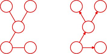
Solution 8.21 67
Figure 5 The graph on the left is an
undirected tree. If we pick
x4to be the root node and
direct all the edges in the
graph to point from the root
to the leaf nodes (x1,x2and
x5), we obtain the directed
tree shown on the right.
x1x2
x3
x4x5
x1x2
x3
x4x5
For a single root node, the required condition holds trivially true, since there are no
messages to be passed. We then assume that it holds for a tree with Nnodes. In the
induction step we add a new leaf node to such a tree. This new leaf node need not
to wait for any messages from other nodes in order to send its outgoing message and
so it can be scheduled to send it first, before any other messages are sent. Its parent
node will receive this message, whereafter the message propagation will follow the
schedule for the original tree with Nnodes, for which the condition is assumed to
hold.
For the propagation of the outward messages from the root back to the leaves, we
first follow the propagation schedule for the original tree with Nnodes, for which
the condition is assumed to hold. When this has completed, the parent of the new
leaf node will be ready to send its outgoing message to the new leaf node, thereby
completing the propagation for the tree with N+ 1 nodes.
8.21 NOTE: In the 1st printing of PRML, this exercise contains a typographical error. On
line 2, fx(xs)should be fs(xs).
To compute p(xs), we marginalize p(x)over all other variables, analogously to
(8.61),
p(xs) = X
x\xs
p(x).
Using (8.59) and the defintion of Fs(x, Xs)that followed (8.62), we can write this
as
p(xs) = X
x\xs
fs(xs)Y
i∈ne(fs)Y
j∈ne(xi)\fs
Fj(xi, Xij )
=fs(xs)Y
i∈ne(fs)X
x\xsY
j∈ne(xi)\fs
Fj(xi, Xij )
=fs(xs)Y
i∈ne(fs)
µxi→fs(xi),
where in the last step, we used (8.67) and (8.68). Note that the marginalization over
the different sub-trees rooted in the neighbours of fswould only run over variables
in the respective sub-trees.

68 Solutions 8.23–9.1
8.23 This follows from the fact that the message that a node, xi, will send to a factor fs,
consists of the product of all other messages received by xi. From (8.63) and (8.69),
we have
p(xi) = Y
s∈ne(xi)
µfs→xi(xi)
=µfs→xi(xi)Y
t∈ne(xi)\fs
µft→xi(xi)
=µfs→xi(xi)µxi→fs(xi).
8.28 If a graph has one or more cycles, there exists at least one set of nodes and edges
such that, starting from an arbitrary node in the set, we can visit all the nodes in the
set and return to the starting node, without traversing any edge more than once.
Consider one particular such cycle. When one of the nodes n1in the cycle sends a
message to one of its neighbours n2in the cycle, this causes a pending messages on
the edge to the next node n3in that cycle. Thus sending a pending message along an
edge in the cycle always generates a pending message on the next edge in that cycle.
Since this is true for every node in the cycle it follows that there will always exist at
least one pending message in the graph.
8.29 We show this by induction over the number of nodes in the tree-structured factor
graph.
First consider a graph with two nodes, in which case only two messages will be sent
across the single edge, one in each direction. None of these messages will induce
any pending messages and so the algorithm terminates.
We then assume that for a factor graph with Nnodes, there will be no pending
messages after a finite number of messages have been sent. Given such a graph, we
can construct a new graph with N+ 1 nodes by adding a new node. This new node
will have a single edge to the original graph (since the graph must remain a tree)
and so if this new node receives a message on this edge, it will induce no pending
messages. A message sent from the new node will trigger propagation of messages
in the original graph with Nnodes, but by assumption, after a finite number of
messages have been sent, there will be no pending messages and the algorithm will
terminate.
Chapter 9 Mixture Models and EM
9.1 Since both the E- and the M-step minimise the distortion measure (9.1), the algorithm
will never change from a particular assignment of data points to prototypes, unless
the new assignment has a lower value for (9.1).
Since there is a finite number of possible assignments, each with a corresponding
unique minimum of (9.1) w.r.t. the prototypes, {µk}, the K-means algorithm will

Solutions 9.3–9.7 69
converge after a finite number of steps, when no re-assignment of data points to
prototypes will result in a decrease of (9.1). When no-reassignment takes place,
there also will not be any change in {µk}.
9.3 From (9.10) and (9.11), we have
p(x) = X
z
p(x|z)p(z) = X
z
K
Y
k=1
(πkN(x|µk,Σk))zk.
Exploiting the 1-of-Krepresentation for z, we can re-write the r.h.s. as
K
X
j=1
K
Y
k=1
(πkN(x|µk,Σk))Ikj =
K
X
j=1
πjN(x|µj,Σj)
where Ikj = 1 if k=jand 0 otherwise.
9.7 Consider first the optimization with respect to the parameters {µk,Σk}. For this we
can ignore the terms in (9.36) which depend on ln πk. We note that, for each data
point n, the quantities znk are all zero except for a particular element which equals
one. We can therefore partition the data set into Kgroups, denoted Xk, such that all
the data points xnassigned to component kare in group Xk. The complete-data log
likelihood function can then be written
ln p(X,Z|µ,Σ,π) =
K
X
k=1 (X
n∈Xk
ln N(xn|µk,Σk)).
This represents the sum of Kindependent terms, one for each component in the
mixture. When we maximize this term with respect to µkand Σkwe will simply
be fitting the kth component to the data set Xk, for which we will obtain the usual
maximum likelihood results for a single Gaussian, as discussed in Chapter 2.
For the mixing coefficients we need only consider the terms in ln πkin (9.36), but
we must introduce a Lagrange multiplier to handle the constraint Pkπk= 1. Thus
we maximize N
X
n=1
K
X
k=1
znk ln πk+λ K
X
k=1
πk−1!
which gives
0 =
N
X
n=1
znk
πk
+λ.
Multiplying through by πkand summing over kwe obtain λ=−N, from which we
have
πk=1
N
N
X
n=1
znk =Nk
N
where Nkis the number of data points in group Xk.

70 Solutions 9.8–9.15
9.8 Using (2.43), we can write the r.h.s. of (9.40) as
−1
2
N
X
n=1
K
X
j=1
γ(znj)(xn−µj)TΣ−1(xn−µj) + const.,
where ‘const.’ summarizes terms independent of µj(for all j). Taking the derivative
of this w.r.t. µk, we get
−
N
X
n=1
γ(znk)Σ−1µk−Σ−1xn,
and setting this to zero and rearranging, we obtain (9.17).
9.12 Since the expectation of a sum is the sum of the expectations we have
E[x] =
K
X
k=1
πkEk[x] =
K
X
k=1
πkµk
where Ek[x]denotes the expectation of xunder the distribution p(x|k). To find the
covariance we use the general relation
cov[x] = E[xxT]−E[x]E[x]T
to give
cov[x] = E[xxT]−E[x]E[x]T
=
K
X
k=1
πkEk[xxT]−E[x]E[x]T
=
K
X
k=1
πkΣk+µkµT
k−E[x]E[x]T.
9.15 This is easily shown by calculating the derivatives of (9.55), setting them to zero and
solve for µki. Using standard derivatives, we get
∂
∂µki
EZ[ln p(X,Z|µ,π)] =
N
X
n=1
γ(znk)xni
µki −1−xni
1−µki
=Pnγ(znk)xni −Pnγ(znk)µki
µki(1 −µki).
Setting this to zero and solving for µki, we get
µki =Pnγ(znk)xni
Pnγ(znk),
which equals (9.59) when written in vector form.

Solutions 9.17–9.25 71
9.17 This follows directly from the equation for the incomplete log-likelihood, (9.51).
The largest value that the argument to the logarithm on the r.h.s. of (9.51) can have
is 1, since ∀n, k : 0 6p(xn|µk)61,06πk61and PK
kπk= 1. Therefore, the
maximum value for ln p(X|µ,π)equals 0.
9.20 If we take the derivatives of (9.62) w.r.t. α, we get
∂
∂αE[ln p(t,w|α, β)] = M
2
1
α−1
2EwTw.
Setting this equal to zero and re-arranging, we obtain (9.63).
9.23 NOTE: In the 1st printing of PRML, the task set in this exercise is to show that the
two sets of re-estimation equations are formally equivalent, without any restriction.
However, it really should be restricted to stationary points of the objective function.
Considering the case when the optimization has converged, we can start with αi, as
defined by (7.87), and use (7.89) to re-write this as
α?
i=1−α?
iΣii
m2
N
,
where α?
i=αnew
i=αiis the value reached at convergence. We can re-write this as
α?
i(m2
i+ Σii) = 1
which is easily re-written as (9.67).
For β, we start from (9.68), which we re-write as
1
β?=kt−ΦmNk2
N+Piγi
β?N.
As in the α-case, β?=βnew =βis the value reached at convergence. We can
re-write this as
1
β? N−X
i
γi!=kt−ΦmNk2,
which can easily be re-written as (7.88).
9.25 This follows from the fact that the Kullback-Leibler divergence, KL(qkp), is at its
minimum, 0, when qand pare identical. This means that
∂
∂θKL(qkp) = 0,
since p(Z|X,θ)depends on θ. Therefore, if we compute the gradient of both sides
of (9.70) w.r.t. θ, the contribution from the second term on the r.h.s. will be 0, and
so the gradient of the first term must equal that of the l.h.s.

72 Solutions 9.26–10.1
9.26 From (9.18) we get
Nold
k=X
n
γold(znk).(137)
We get Nnew
kby recomputing the responsibilities, γ(zmk), for a specific data point,
xm, yielding
Nnew
k=X
n=m
γold(znk) + γnew(zmk ).(138)
Combining this with (137), we get (9.79).
Similarly, from (9.17) we have
µold
k=1
Nold
kX
n
γold(znk)xn
and recomputing the responsibilities, γ(zmk), we get
µnew
k=1
Nnew
k X
n=m
γold(znk)xn+γnew(zmk)xm!
=1
Nnew
kNold
kµold
k−γold(zmk)xm+γnew(zmk)xm
=1
Nnew
kNnew
k−γnew(zmk) + γold(zmk)µold
k
−γold(zmk)xm+γnew(zmk)xm
=µold
k+γnew(zmk)−γold(zmk)
Nnew
k(xm−µold
k),
where we have used (9.79).
Chapter 10 Approximate Inference
10.1 Starting from (10.3), we use the product rule together with (10.4) to get
L(q) = Zq(Z) ln p(X,Z)
q(Z)dZ
=Zq(Z) ln p(X|Z)p(X)
q(Z)dZ
=Zq(Z)ln p(X|Z)
q(Z)+ ln p(X)dZ
=−KL( qkp) + ln p(X).
Rearranging this, we immediately get (10.2).

Solution 10.3 73
10.3 Starting from (10.16) and optimizing w.r.t. qj(Zj), we get
KL( pkq) = −Zp(Z)"M
X
i=1
ln qi(Zi)#dZ+ const.
=−Z p(Z) ln qj(Zj) + p(Z)X
i=j
ln qi(Zi)!dZ+ const.
=−Zp(Z) ln qj(Zj) dZ+ const.
=−Zln qj(Zj)"Zp(Z)Y
i=j
dZi#dZj+ const.
=−ZFj(Zj) ln qj(Zj) dZj+ const.,
where terms independent of qj(Zj)have been absorbed into the constant term and
we have defined
Fj(Zj) = Zp(Z)Y
i=j
dZi.
We use a Lagrange multiplier to ensure that qj(Zj)integrates to one, yielding
−ZFj(Zj) ln qj(Zj) dZj+λZqj(Zj) dZj−1.
Using the results from Appendix D, we then take the functional derivative of this
w.r.t. qjand set this to zero, to obtain
−Fj(Zj)
qj(Zj)+λ= 0.
From this, we see that
λqj(Zj) = Fj(Zj).
Integrating both sides over Zj, we see that, since qj(Zj)must intgrate to one,
λ=ZFj(Zj) dZj=Z"Zp(Z)Y
i=j
dZi#dZj= 1,
and thus
qj(Zj) = Fj(Zj) = Zp(Z)Y
i=j
dZi.

74 Solutions 10.5–10.10
10.5 We assume that q(Z) = q(z)q(θ)and so we can optimize w.r.t. q(z)and q(θ)inde-
pendently.
For q(z), this is equivalent to minimizing the Kullback-Leibler divergence, (10.4),
which here becomes
KL( qkp) = −ZZ q(θ)q(z) ln p(z,θ|X)
q(z)q(θ)dzdθ.
For the particular chosen form of q(θ), this is equivalent to
KL( qkp) = −Zq(z) ln p(z,θ0|X)
q(z)dz+ const.
=−Zq(z) ln p(z|θ0,X)p(θ0|X)
q(z)dz+ const.
=−Zq(z) ln p(z|θ0,X)
q(z)dz+ const.,
where const accumulates all terms independent of q(z). This KL divergence is min-
imized when q(z) = p(z|θ0,X), which corresponds exactly to the E-step of the EM
algorithm.
To determine q(θ), we consider
Zq(θ)Zq(z) ln p(X,θ,z)
q(θ)q(z)dzdθ
=Zq(θ)Eq(z)[ln p(X,θ,z)] dθ−Zq(θ) ln q(θ) dθ+ const.
where the last term summarizes terms independent of q(θ). Since q(θ)is con-
strained to be a point density, the contribution from the entropy term (which formally
diverges) will be constant and independent of θ0. Thus, the optimization problem is
reduced to maximizing expected complete log posterior distribution
Eq(z)[ln p(X,θ0,z)] ,
w.r.t. θ0, which is equivalent to the M-step of the EM algorithm.
10.10 NOTE: In the 1st printing of PRML, there are errors that affect this exercise. Lm
used in (10.34) and (10.35) should really be L, whereas Lmused in (10.36) is given
in Solution 10.11 below.
This completely analogous to Solution 10.1. Starting from (10.35), we can use the

Solution 10.11 75
product rule to get,
L=X
mX
Z
q(Z|m)q(m) ln p(Z,X, m)
q(Z|m)q(m)
=X
mX
Z
q(Z|m)q(m) ln p(Z, m|X)p(X)
q(Z|m)q(m)
=X
mX
Z
q(Z|m)q(m) ln p(Z, m|X)
q(Z|m)q(m)+ ln p(X).
Rearranging this, we obtain (10.34).
10.11 NOTE: Consult note preceding Solution 10.10 for some relevant corrections.
We start by rewriting the lower bound as follows
L=X
mX
Z
q(Z|m)q(m) ln p(Z,X, m)
q(Z|m)q(m)
=X
mX
Z
q(Z|m)q(m){ln p(Z,X|m) + ln p(m)−ln q(Z|m)−ln q(m)}
=X
m
q(m)ln p(m)−ln q(m)
+X
Z
q(Z|m){ln p(Z,X|m)−ln q(Z|m)}
=X
m
q(m){ln (p(m) exp{Lm})−ln q(m)},(139)
where
Lm=X
Z
q(Z|m) ln p(Z,X|m)
q(Z|m).
We recognize (139) as the negative KL divergence between q(m)and the (not nec-
essarily normalized) distribution p(m) exp{Lm}. This will be maximized when the
KL divergence is minimized, which will be the case when
q(m)∝p(m) exp{Lm}.

76 Solution 10.13
10.13 In order to derive the optimal solution for q(µk,Λk)we start with the result (10.54)
and keep only those term which depend on µkor Λkto give
ln q?(µk,Λk) = ln Nµk|m0,(β0Λk)−1+ ln W(Λk|W0, ν0)
+
N
X
n=1
E[znk] ln Nxn|µk,Λ−1
k+ const.
=−β0
2(µk−m0)TΛk(µk−m0) + 1
2ln |Λk| − 1
2Tr ΛkW−1
0
+(ν0−D−1)
2ln |Λk| − 1
2
N
X
n=1
E[znk](xn−µk)TΛk(xn−µk)
+1
2 N
X
n=1
E[znk]!ln |Λk|+ const.(140)
Using the product rule of probability, we can express ln q?(µk,Λk)as ln q?(µk|Λk)
+ ln q?(Λk). Let us first of all identify the distribution for µk. To do this we need
only consider terms on the right hand side of (140) which depend on µk, giving
ln q?(µk|Λk)
=−1
2µT
k"β0+
N
X
n=1
E[znk]#Λkµk+µT
kΛk"β0m0+
N
X
n=1
E[znk]xn#
+const.
=−1
2µT
k[β0+Nk]Λkµk+µT
kΛk[β0m0+Nkxk] + const.
where we have made use of (10.51) and (10.52). Thus we see that ln q?(µk|Λk)
depends quadratically on µkand hence q?(µk|Λk)is a Gaussian distribution. Com-
pleting the square in the usual way allows us to determine the mean and precision of
this Gaussian, giving
q?(µk|Λk) = N(µk|mk, βkΛk)(141)
where
βk=β0+Nk
mk=1
βk
(β0m0+Nkxk).
Next we determine the form of q?(Λk)by making use of the relation
ln q?(Λk) = ln q?(µk,Λk)−ln q?(µk|Λk).
On the right hand side of this relation we substitute for ln q?(µk,Λk)using (140),
and we substitute for ln q?(µk|Λk)using the result (141). Keeping only those terms

Solution 10.16 77
which depend on Λkwe obtain
ln q?(Λk) = −β0
2(µk−m0)TΛk(µk−m0) + 1
2ln |Λk| − 1
2Tr ΛkW−1
0
+(ν0−D−1)
2ln |Λk| − 1
2
N
X
n=1
E[znk](xn−µk)TΛk(xn−µk)
+1
2 N
X
n=1
E[znk]!ln |Λk|+βk
2(µk−mk)TΛk(µk−mk)
−1
2ln |Λk|+ const.
=(νk−D−1)
2ln |Λk| − 1
2Tr ΛkW−1
k+ const.
Here we have defined
W−1
k=W−1
0+β0(µk−m0)(µk−m0)T+
N
X
n=1
E[znk](xn−µk)(xn−µk)T
−βk(µk−mk)(µk−mk)T
=W−1
0+NkSk+β0Nk
β0+Nk
(xk−m0)(xk−m0)T(142)
νk=ν0+
N
X
n=1
E[znk]
=ν0+Nk,
where we have made use of the result
N
X
n=1
E[znk]xnxT
n=
N
X
n=1
E[znk](xn−xk)(xn−xk)T+NkxkxT
k
=NkSk+NkxkxT
k(143)
and we have made use of (10.53). Note that the terms involving µkhave cancelled
out in (142) as we expect since q?(Λk)is independent of µk.
Thus we see that q?(Λk)is a Wishart distribution of the form
q?(Λk) = W(Λk|Wk, νk).
10.16 To derive (10.71) we make use of (10.38) to give
E[ln p(D|z,µ,Λ)]
=1
2
N
X
n=1
K
X
k=1
E[znk]{E[ln |Λk|]−E[(xn−µk)Λk(xn−µk)] −Dln(2π)}.

78 Solution 10.20
We now use E[znk] = rnk together with (10.64) and the definition of e
Λkgiven by
(10.65) to give
E[ln p(D|z,µ,Λ)] = 1
2
N
X
n=1
K
X
k=1
rnkln e
Λk
−Dβ−1
k−νk(xn−mk)TWk(xn−mk)−Dln(2π).
Now we use the definitions (10.51) to (10.53) together with the result (143) to give
(10.71).
We can derive (10.72) simply by taking the logarithm of p(z|π)given by (10.37)
E[ln p(z|π)] =
N
X
n=1
K
X
k=1
E[znk]E[ln πk]
and then making use of E[znk] = rnk together with the definition of eπkgiven by
(10.65).
10.20 Consider first the posterior distribution over the precision of component kgiven by
q?(Λk) = W(Λk|Wk, νk).
From (10.63) we see that for large Nwe have νk→Nk, and similarly from (10.62)
we see that Wk→N−1
kS−1
k. Thus the mean of the distribution over Λk, given by
E[Λk] = νkWk→S−1
kwhich is the maximum likelihood value (this assumes that
the quantities rnk reduce to the corresponding EM values, which is indeed the case
as we shall show shortly). In order to show that this posterior is also sharply peaked,
we consider the differential entropy, H[Λk]given by (B.82), and show that, as Nk→
∞,H[Λk]→0, corresponding to the density collapsing to a spike. First consider
the normalizing constant B(Wk, νk)given by (B.79). Since Wk→N−1
kS−1
kand
νk→Nk,
−ln B(Wk, νk)→ −Nk
2(Dln Nk+ ln |Sk| − Dln 2)+
D
X
i=1
ln Γ Nk+ 1 −i
2.
We then make use of Stirling’s approximation (1.146) to obtain
ln Γ Nk+ 1 −i
2'Nk
2(ln Nk−ln 2 −1)
which leads to the approximate limit
−ln B(Wk, νk)→ −NkD
2(ln Nk−ln 2 −ln Nk+ ln 2 + 1) −Nk
2ln |Sk|
=−Nk
2(ln |Sk|+D).(144)

Solution 10.23 79
Next, we use (10.241) and (B.81) in combination with Wk→N−1
kS−1
kand νk→
Nkto obtain the limit
E[ln |Λ|]→Dln Nk
2+Dln 2 −Dln Nk−ln |Sk|
=−ln |Sk|,
where we approximated the argument to the digamma function by Nk/2. Substitut-
ing this and (144) into (B.82), we get
H[Λ]→0
when Nk→ ∞.
Next consider the posterior distribution over the mean µkof the kth component given
by
q?(µk|Λk) = N(µk|mk, βkΛk).
From (10.61) we see that for large Nthe mean mkof this distribution reduces to
xkwhich is the corresponding maximum likelihood value. From (10.60) we see that
βk→Nkand Thus the precision βkΛk→βkνkWk→NkS−1
kwhich is large for
large Nand hence this distribution is sharply peaked around its mean.
Now consider the posterior distribution q?(π)given by (10.57). For large Nwe
have αk→Nkand so from (B.17) and (B.19) we see that the posterior distribution
becomes sharply peaked around its mean E[πk] = αk/α →Nk/N which is the
maximum likelihood solution.
For the distribution q?(z)we consider the responsibilities given by (10.67). Using
(10.65) and (10.66), together with the asymptotic result for the digamma function,
we again obtain the maximum likelihood expression for the responsibilities for large
N.
Finally, for the predictive distribution we first perform the integration over π, as in
the solution to Exercise 10.19, to give
p(bx|D) =
K
X
k=1
αk
αZZ N(bx|µk,Λk)q(µk,Λk) dµkdΛk.
The integrations over µkand Λkare then trivial for large Nsince these are sharply
peaked and hence approximate delta functions. We therefore obtain
p(bx|D) =
K
X
k=1
Nk
NN(bx|xk,Wk)
which is a mixture of Gaussians, with mixing coefficients given by Nk/N.
10.23 When we are treating πas a parameter, there is neither a prior, nor a variational
posterior distribution, over π. Therefore, the only term remaining from the lower

80 Solution 10.24
bound, (10.70), that involves πis the second term, (10.72). Note however, that
(10.72) involves the expectations of ln πkunder q(π), whereas here, we operate
directly with πk, yielding
Eq(Z)[ln p(Z|π)] =
N
X
n=1
K
X
k=1
rnk ln πk.
Adding a Langrange term, as in (9.20), taking the derivative w.r.t. πkand setting the
result to zero we get Nk
πk
+λ= 0,(145)
where we have used (10.51). By re-arranging this to
Nk=−λπk
and summing both sides over k, we see that −λ=PkNk=N, which we can use
to eliminate λfrom (145) to get (10.83).
10.24 The singularities that may arise in maximum likelihood estimation are caused by a
mixture component, k, collapsing on a data point, xn, i.e., rkn = 1,µk=xnand
|Λk| → ∞.
However, the prior distribution p(µ,Λ)defined in (10.40) will prevent this from
happening, also in the case of MAP estimation. Consider the product of the expected
complete log-likelihood and p(µ,Λ)as a function of Λk:
Eq(Z)[ln p(X|Z,µ,Λ)p(µ,Λ)]
=1
2
N
X
n=1
rkn ln |Λk| − (xn−µk)TΛk(xn−µk)
+ ln |Λk| − β0(µk−m0)TΛk(µk−m0)
+(ν0−D−1) ln |Λk| − Tr W−1
0Λk+ const.
where we have used (10.38), (10.40) and (10.50), together with the definitions for
the Gaussian and Wishart distributions; the last term summarizes terms independent
of Λk. Using (10.51)–(10.53), we can rewrite this as
(ν0+Nk−D) ln |Λk| − Tr (W−1
0+β0(µk−m0)(µk−m0)T+NkSk)Λk,
where we have dropped the constant term. Using (C.24) and (C.28), we can compute
the derivative of this w.r.t. Λkand setting the result equal to zero, we find the MAP
estimate for Λkto be
Λ−1
k=1
ν0+Nk−D(W−1
0+β0(µk−m0)(µk−m0)T+NkSk).
From this we see that |Λ−1
k|can never become 0, because of the presence of W−1
0
(which we must chose to be positive definite) in the expression on the r.h.s.

Solutions 10.29–10.32 81
10.29 NOTE: In the 1st printing of PRML, the use of λto denote the varitional param-
eter leads to inconsistencies w.r.t. exisiting literature. To remedy this λshould be
replaced by ηfrom the beginning of Section 10.5 up to and including the last line
before equation (10.141). For further details, please consult the PRML Errata.
Standard rules of differentiation give
dln(x)
dx =1
x
d2ln(x)
dx2=−1
x2.
Since its second derivative is negative for all value of x,ln(x)is concave for 0<
x < ∞.
From (10.133) we have
g(η) = min
x{ηx −f(x)}
= min
x{ηx −ln(x)}.
We can minimize this w.r.t. xby setting the corresponding derivative to zero and
solving for x:dg
dx =η−1
x= 0 =⇒x=1
η.
Substituting this in (10.133), we see that
g(η) = 1 −ln 1
η.
If we substitute this into (10.132), we get
f(x) = min
ηηx −1 + ln 1
η.
Again, we can minimize this w.r.t. ηby setting the corresponding derivative to zero
and solving for η:df
dη =x−1
η= 0 =⇒η=1
x,
and substituting this into (10.132), we find that
f(x) = 1
xx−1 + ln 1
1/x= ln(x).
10.32 We can see this from the lower bound (10.154), which is simply a sum of the prior
and indepedent contributions from the data points, all of which are quadratic in w. A
new data point would simply add another term to this sum and we can regard terms
82 Solution 10.37
from the previously arrived data points and the original prior collectively as a revised
prior, which should be combined with the contributions from the new data point.
The corresponding sufficient statistics, (10.157) and (10.158), can be rewritten di-
rectly in the corresponding sequential form,
mN=SN S−1
0m0+
N
X
n=1
(tn−1/2)φn!
=SN S−1
0m0+
N−1
X
n=1
(tn−1/2)φn+ (tN−1/2)φN!
=SN S−1
N−1SN−1 S−1
0m0+
N−1
X
n=1
(tn−1/2)φn!+ (tN−1/2)φN!
=SNS−1
N−1mN−1+ (tN−1/2)φN
and
S−1
N=S−1
0+ 2
N
X
n=1
λ(ξn)φnφT
n
=S−1
0+ 2
N−1
X
n=1
λ(ξn)φnφT
n+ 2λ(ξN)φNφT
N
=S−1
N−1+ 2λ(ξN)φNφT
N.
The update formula for the variational parameters, (10.163), remain the same, but
each parameter is updated only once, although this update will be part of an iterative
scheme, alternating between updating mNand SNwith ξNkept fixed, and updating
ξNwith mNand SNkept fixed. Note that updating ξNwill not affect mN−1and
SN−1. Note also that this updating policy differs from that of the batch learning
scheme, where all variational parameters are updated using statistics based on all
data points.
10.37 Here we use the general expectation-propagation equations (10.204)–(10.207). The
initial q(θ)takes the form
qinit(θ) = e
f0(θ)Y
i=0 e
fi(θ)
where e
f0(θ) = f0(θ). Thus
q\0(θ)∝Y
i=0 e
fi(θ)
and qnew(θ)is determined by matching moments (sufficient statistics) against
q\0(θ)f0(θ) = qinit(θ).

Solution 11.1 83
Since by definition this belongs to the same exponential family form as qnew(θ)it
follows that
qnew(θ) = qinit(θ) = q\0(θ)f0(θ).
Thus
e
f0(θ) = Z0qnew(θ)
q\0(θ)=Z0f0(θ)
where
Z0=Zq\0(θ)f0(θ) dθ=Zqnew(θ) dθ= 1.
Chapter 11 Sampling Methods
11.1 Since the samples are independent, for the mean, we have
Ehb
fi=1
L
L
X
l=1 Zf(z(l))p(z(l)) dz(l)=1
L
L
X
l=1
E[f] = E[f].
Using this together with (1.38) and (1.39), for the variance, we have
var hb
fi=Eb
f−Ehb
fi2
=Ehb
f2i−E[f]2.
Now note
Ef(z(k)), f(z(m))=var[f] + E[f2]if n=k,
E[f2]otherwise,
=E[f2] + δmkvar[f],
where we again exploited the fact that the samples are independent.
Hence
var hb
fi=E"1
L
L
X
m=1
f(z(m))1
L
L
X
k=1
f(z(k))#−E[f]2
=1
L2
L
X
m=1
L
X
k=1 E[f2] + δmkvar[f]−E[f]2
=1
Lvar[f]
=1
LE(f−E[f])2.

84 Solutions 11.5–11.11
11.5 Since E[z] = 0,
E[y] = E[µ+Lz] = µ.
Similarly, since EzzT=I,
cov [y] = EyyT−E[y]EyT
=Eh(µ+Lz) (µ+Lz)Ti−µµT
=LLT
=Σ.
11.6 The probability of acceptance follows directly from the mechanism used to accept or
reject the sample. The probability of a sample zbeing accepted equals the probability
of a sample u, drawn uniformly from the interval [0, kq(z)], being less than or equal
to a value ep(z)6kq(z), and is given by is given by
p(acceptance|z) = Zep(z)
0
1
kq(z)du=ep(z)
kq(z).
Therefore, the probability of drawing a sample, z, is
q(z)p(acceptance|z) = q(z)ep(z)
kq(z)=ep(z)
k.(146)
Integrating both sides w.r.t. z, we see that kp(acceptance) = Zp, where
Zp=Zep(z) dz.
Combining this with (146) and (11.13), we obtain
q(z)p(acceptance|z)
p(acceptance) =1
Zpep(z) = p(z)
as required.
11.11 This follows from the fact that in Gibbs sampling, we sample a single variable, zk,
at the time, while all other variables, {zi}i=k, remain unchanged. Thus, {z
i}i=k=
{zi}i=kand we get
p?(z)T(z,z) = p?(zk,{zi}i=k)p?(z
k|{zi}i=k)
=p?(zk|{zi}i=k)p?({zi}i=k)p?(z
k|{zi}i=k)
=p?(zk|{z
i}i=k)p?({z
i}i=k)p?(z
k|{z
i}i=k)
=p?(zk|{z
i}i=k)p?(z
k,{z
i}i=k)
=p?(z)T(z,z),
where we have used the product rule together with T(z,z) = p?(z
k|{zi}i=k).

Solutions 11.15–12.1 85
11.15 Using (11.56), we can differentiate (11.57), yielding
∂H
∂ri
=∂K
∂ri
=ri
and thus (11.53) and (11.58) are equivalent.
Similarly, differentiating (11.57) w.r.t. ziwe get
∂H
∂zi
=∂E
∂zi
,
and from this, it is immediately clear that (11.55) and (11.59) are equivalent.
11.17 NOTE: In the 1st printing of PRML, there are sign errors in equations (11.68) and
(11.69). In both cases, the sign of the argument to the exponential forming the second
argument to the min-function should be changed.
First we note that, if H(R) = H(R), then the detailed balance clearly holds, since
in this case, (11.68) and (11.69) are identical.
Otherwise, we either have H(R)> H(R)or H(R)< H(R). We consider the
former case, for which (11.68) becomes
1
ZH
exp(−H(R))δV 1
2,
since the min-function will return 1. (11.69) in this case becomes
1
ZH
exp(−H(R))δV 1
2exp(H(R)−H(R)) = 1
ZH
exp(−H(R))δV 1
2.
In the same way it can be shown that both (11.68) and (11.69) equal
1
ZH
exp(−H(R))δV 1
2
when H(R)< H(R).
Chapter 12 Continuous Latent Variables
12.1 Suppose that the result holds for projection spaces of dimensionality M. The M+
1dimensional principal subspace will be defined by the Mprincipal eigenvectors
u1,...,uMtogether with an additional direction vector uM+1 whose value we wish
to determine. We must constrain uM+1 such that it cannot be linearly related to
u1,...,uM(otherwise it will lie in the M-dimensional projection space instead of
defining an M+ 1 independent direction). This can easily be achieved by requiring
that uM+1 be orthogonal to u1,...,uM, and these constraints can be enforced using
Lagrange multipliers η1,...,ηM.
86 Solutions 12.4–12.6
Following the argument given in section 12.1.1 for u1we see that the variance in the
direction uM+1 is given by uT
M+1SuM+1. We now maximize this using a Lagrange
multiplier λM+1 to enforce the normalization constraint uT
M+1uM+1 = 1. Thus we
seek a maximum of the function
uT
M+1SuM+1 +λM+1 1−uT
M+1uM+1+
M
X
i=1
ηiuT
M+1ui.
with respect to uM+1. The stationary points occur when
0 = 2SuM+1 −2λM+1uM+1 +
M
X
i=1
ηiui.
Left multiplying with uT
j, and using the orthogonality constraints, we see that ηj= 0
for j= 1, . . . , M. We therefore obtain
SuM+1 =λM+1uM+1
and so uM+1 must be an eigenvector of Swith eigenvalue uM+1. The variance
in the direction uM+1 is given by uT
M+1SuM+1 =λM+1 and so is maximized by
choosing uM+1 to be the eigenvector having the largest eigenvalue amongst those
not previously selected. Thus the result holds also for projection spaces of dimen-
sionality M+ 1, which completes the inductive step. Since we have already shown
this result explicitly for M= 1 if follows that the result must hold for any M6D.
12.4 Using the results of Section 8.1.4, the marginal distribution for this modified proba-
bilistic PCA model can be written
p(x) = N(x|Wm +µ, σ2I+WTΣ−1W).
If we now define new parameters
f
W=Σ1/2W
eµ=Wm +µ
then we obtain a marginal distribution having the form
p(x) = N(x|eµ, σ2I+f
WTf
W).
Thus any Gaussian form for the latent distribution therefore gives rise to a predictive
distribution having the same functional form, and so for convenience we choose the
simplest form, namely one with zero mean and unit covariance.
12.6 Omitting the parameters, W,µand σ, leaving only the stochastic variables zand
x, the graphical model for probabilistic PCA is identical with the the ‘naive Bayes’
model shown in Figure 8.24 in Section 8.2.2. Hence these two models exhibit the
same independence structure.

Solutions 12.8–12.15 87
12.8 NOTE: In the 1st printing of PRML, equation (12.42) contains a mistake; the co-
variance on the r.h.s. should be σ2M−1.
By matching (12.31) with (2.113) and (12.32) with (2.114), we have from (2.116)
and (2.117) that
p(z|x) = Nz|(I+σ−2WTW)−1WTσ−2I(x−µ),(I+σ−2WTW)−1
=Nz|M−1WT(x−µ), σ2M−1,
where we have also used (12.41).
12.11 Taking σ2→0in (12.41) and substituting into (12.48) we obtain the posterior mean
for probabilistic PCA in the form
(WT
MLWML)−1WT
ML(x−x).
Now substitute for WML using (12.45) in which we take R=Ifor compatibility
with conventional PCA. Using the orthogonality property UT
MUM=Iand setting
σ2= 0, this reduces to
L−1/2UT
M(x−x)
which is the orthogonal projection is given by the conventional PCA result (12.24).
12.15 NOTE: In PRML, a term M/2 ln(2π)is missing from the summand on the r.h.s. of
(12.53). However, this is only stated here for completeness as it actually does not
affect this solution.
Using standard derivatives together with the rules for matrix differentiation from
Appendix C, we can compute the derivatives of (12.53) w.r.t. Wand σ2:
∂
∂WE[ln pX,Z|µ,W, σ2] =
N
X
n=1 1
σ2(xn−x)E[zn]T−1
σ2WE[znzT
n]
and
∂
∂σ2E[ln pX,Z|µ,W, σ2] =
N
X
n=1 1
2σ4E[znzT
n]WTW
+1
2σ4kxn−xk2−1
σ4E[zn]TWT(xn−x)−D
2σ2
Setting these equal to zero and re-arranging we obtain (12.56) and (12.57), respec-
tively.

88 Solutions 12.17–12.25
12.17 NOTE: In PRML, there are errors in equation (12.58) and the preceding text. In
(12.58), e
Xshould be e
XTand in the preceding text we define Ωto be a matrix of size
M×Nwhose nth column is given by the vector E[zn].
Setting the derivative of Jwith respect to µto zero gives
0 = −
N
X
n=1
(xn−µ−Wzn)
from which we obtain
µ=1
N
N
X
n=1
xn−1
N
N
X
n=1
Wzn=x−Wz.
Back-substituting into Jwe obtain
J=
N
X
n=1 k(xn−x−W(zn−z)k2.
We now define Xto be a matrix of size N×Dwhose nth row is given by the vector
xn−xand similarly we define Zto be a matrix of size D×Mwhose nth row is
given by the vector zn−z. We can then write Jin the form
J=Tr (X−ZWT)(X−ZWT)T.
Differentiating with respect to Zkeeping Wfixed gives rise to the PCA E-step
(12.58). Similarly setting the derivative of Jwith respect to Wto zero with {zn}
fixed gives rise to the PCA M-step (12.59).
12.19 To see this we define a rotated latent space vector ez=Rz where Ris an M×Mor-
thogonal matrix, and similarly defining a modified factor loading matrix f
W=WR.
Then we note that the latent space distribution p(z)depends only on zTz=ezTez,
where we have used RTR=I. Similarly, the conditional distribution of the ob-
served variable p(x|z)depends only on Wz =f
Wez. Thus the joint distribution
takes the same form for any choice of R. This is reflected in the predictive distri-
bution p(x)which depends on Wonly through the quantity WWT=f
Wf
WTand
hence is also invariant to different choices of R.
12.23 The solution is given in figure 6. The model in which all parameters are shared (left)
is not particularly useful, since all mixture components will have identical param-
eters and the resulting density model will not be any different to one offered by a
single PPCA model. Different models would have arisen if only some of the param-
eters, e.g. the mean µ, would have been shared.
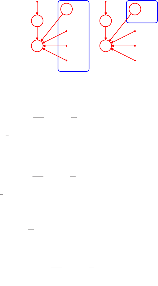
Solution 12.25 89
Figure 6 The left plot shows the
graphical model correspond-
ing to the general mixture of
probabilistic PCA. The right
plot shows the correspond-
ing model were the param-
eter of all probabilist PCA
models (µ,Wand σ2) are
shared across components.
In both plots, sdenotes
the K-nomial latent variable
that selects mixture compo-
nents; it is governed by the
parameter, π.
zk
Wk
µk
σ2
kK
x
s
π
zk
K
W
µ
σ2
x
s
π
12.25 Following the discussion of section 12.2, the log likelihood function for this model
can be written as
L(µ,W,Φ) = −ND
2ln(2π)−N
2ln |WWT+Φ|
−1
2
N
X
n=1 (xn−µ)T(WWT+Φ)−1(xn−µ),
where we have used (12.43).
If we consider the log likelihood function for the transformed data set we obtain
LA(µ,W,Φ) = −ND
2ln(2π)−N
2ln |WWT+Φ|
−1
2
N
X
n=1 (Axn−µ)T(WWT+Φ)−1(Axn−µ).
Solving for the maximum likelihood estimator for µin the usual way we obtain
µA=1
N
N
X
n=1
Axn=Ax =AµML.
Back-substituting into the log likelihood function, and using the definition of the
sample covariance matrix (12.3), we obtain
LA(µ,W,Φ) = −ND
2ln(2π)−N
2ln |WWT+Φ|
−1
2
N
X
n=1
Tr (WWT+Φ)−1ASAT.
We can cast the final term into the same form as the corresponding term in the origi-
nal log likelihood function if we first define
ΦA=AΦ−1AT,WA=AW.

90 Solutions 12.28–12.29
With these definitions the log likelihood function for the transformed data set takes
the form
LA(µA,WA,ΦA) = −ND
2ln(2π)−N
2ln |WAWT
A+ΦA|
−1
2
N
X
n=1 (xn−µA)T(WAWT
A+ΦA)−1(xn−µA)−Nln |A|.
This takes the same form as the original log likelihood function apart from an addi-
tive constant −ln |A|. Thus the maximum likelihood solution in the new variables
for the transformed data set will be identical to that in the old variables.
We now ask whether specific constraints on Φwill be preserved by this re-scaling. In
the case of probabilistic PCA the noise covariance Φis proportional to the unit ma-
trix and takes the form σ2I. For this constraint to be preserved we require AAT=I
so that Ais an orthogonal matrix. This corresponds to a rotation of the coordinate
system. For factor analysis Φis a diagonal matrix, and this property will be pre-
served if Ais also diagonal since the product of diagonal matrices is again diagonal.
This corresponds to an independent re-scaling of the coordinate system. Note that in
general probabilistic PCA is not invariant under component-wise re-scaling and fac-
tor analysis is not invariant under rotation. These results are illustrated in Figure 7.
12.28 If we assume that the function y=f(x)is strictly monotonic, which is necessary to
exclude the possibility for spikes of infinite density in p(y), we are guaranteed that
the inverse function x=f−1(y)exists. We can then use (1.27) to write
p(y) = q(f−1(y))
df−1
dy.(147)
Since the only restriction on fis that it is monotonic, it can distribute the probability
mass over xarbitrarily over y. This is illustrated in Figure 1 on page 8, as a part of
Solution 1.4. From (147) we see directly that
|f(x)|=q(x)
p(f(x)).
12.29 NOTE: In the 1st printing of PRML, this exercise contains two mistakes. In the
second half of the exercise, we require that y1is symmetrically distributed around 0,
not just that −16y161. Moreover, y2=y2
1(not y2=y2
2).
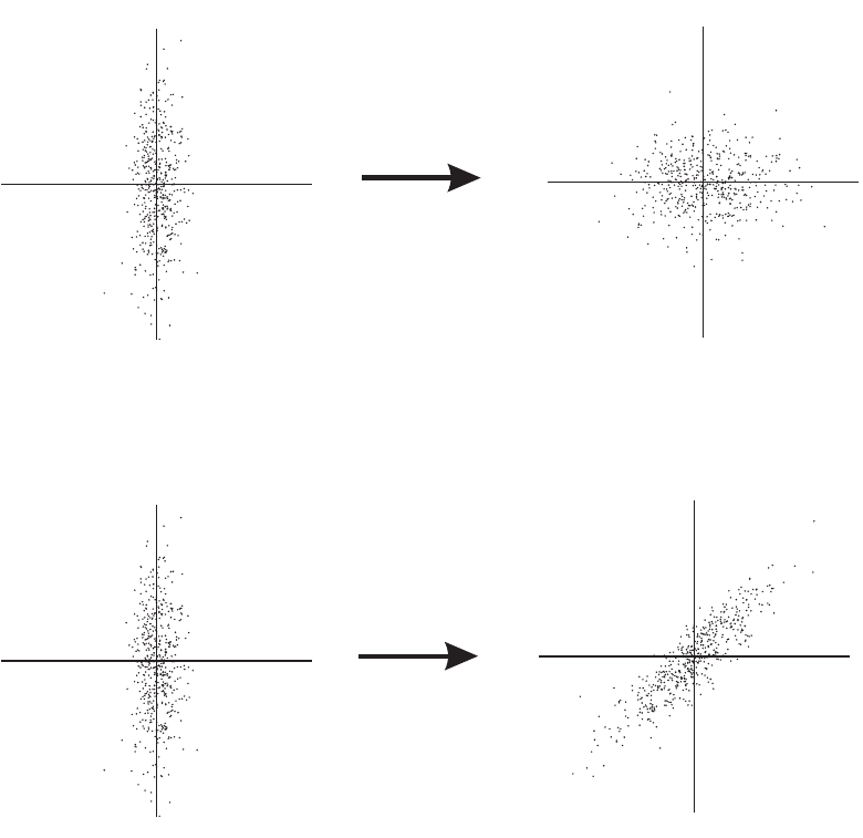
Solution 12.29 91
Figure 7 Factor analysis is covariant under a componentwise re-scaling of the data variables (top plots), while
PCA and probabilistic PCA are covariant under rotations of the data space coordinates (lower plots).

92 Solutions 13.1–13.4
If z1and z2are independent, then
cov[z1, z2] = ZZ(z1−¯z1)(z2−¯z2)p(z1, z2) dz1dz2
=ZZ(z1−¯z1)(z2−¯z2)p(z1)p(z2) dz1dz2
=Z(z1−¯z1)p(z1) dz1Z(z2−¯z2)p(z2) dz2
= 0,
where
¯zi=E[zi] = Zzip(zi) dzi.
For y2we have
p(y2|y1) = δ(y2−y2
1),
i.e., a spike of probability mass one at y2
1, which is clearly dependent on y1. With ¯yi
defined analogously to ¯ziabove, we get
cov[y1, y2] = ZZ(y1−¯y1)(y2−¯y2)p(y1, y2) dy1dy2
=ZZ y1(y2−¯y2)p(y2|y1)p(y1) dy1dy2
=Z(y3
1−y1¯y2)p(y1) dy1
= 0,
where we have used the fact that all odd moments of y1will be zero, since it is
symmetric around zero.
Chapter 13 Sequential Data
13.1 Since the arrows on the path from xmto xn, with m < n −1, will meet head-to-tail
at xn−1, which is in the conditioning set, all such paths are blocked by xn−1and
hence (13.3) holds.
The same argument applies in the case depicted in Figure 13.4, with the modification
that m < n −2and that paths are blocked by xn−1or xn−2.
13.4 The learning of wwould follow the scheme for maximum learning described in
Section 13.2.1, with wreplacing φ. As discussed towards the end of Section 13.2.1,
the precise update formulae would depend on the form of regression model used and
how it is being used.

Solution 13.8 93
The most obvious situation where this would occur is in a HMM similar to that
depicted in Figure 13.18, where the emmission densities not only depends on the
latent variable z, but also on some input variable u. The regression model could
then be used to map uto x, depending on the state of the latent variable z.
Note that when a nonlinear regression model, such as a neural network, is used, the
M-step for wmay not have closed form.
13.8 Only the final term of Q(θ,θold given by (13.17) depends on the parameters of the
emission model. For the multinomial variable x, whose Dcomponents are all zero
except for a single entry of 1,
N
X
n=1
K
X
k=1
γ(znk) ln p(xn|φk) =
N
X
n=1
K
X
k=1
γ(znk)
D
X
i=1
xni ln µki.
Now when we maximize with respect to µki we have to take account of the con-
straints that, for each value of kthe components of µki must sum to one. We there-
fore introduce Lagrange multipliers {λk}and maximize the modified function given
by
N
X
n=1
K
X
k=1
γ(znk)
D
X
i=1
xni ln µki +
K
X
k=1
λk D
X
i=1
µki −1!.
Setting the derivative with respect to µki to zero we obtain
0 =
N
X
n=1
γ(znk)xni
µki
+λk.
Multiplying through by µki, summing over i, and making use of the constraint on
µki together with the result Pixni = 1 we have
λk=−
N
X
n=1
γ(znk).
Finally, back-substituting for λkand solving for µki we again obtain (13.23).
Similarly, for the case of a multivariate Bernoulli observed variable xwhose Dcom-
ponents independently take the value 0 or 1, using the standard expression for the
multivariate Bernoulli distribution we have
N
X
n=1
K
X
k=1
γ(znk) ln p(xn|φk)
=
N
X
n=1
K
X
k=1
γ(znk)
D
X
i=1 {xni ln µki + (1 −xni) ln(1 −µki)}.

94 Solutions 13.9–13.13
Maximizing with respect to µki we obtain
µki =
N
X
n=1
γ(znk)xni
N
X
n=1
γ(znk)
which is equivalent to (13.23).
13.9 We can verify all these independence properties using d-separation by refering to
Figure 13.5.
(13.24) follows from the fact that arrows on paths from any of x1,...,xnto any of
xn+1,...,xNmeet head-to-tail or tail-to-tail at zn, which is in the conditioning set.
(13.25) follows from the fact that arrows on paths from any of x1,...,xn−1to xn
meet head-to-tail at zn, which is in the conditioning set.
(13.26) follows from the fact that arrows on paths from any of x1,...,xn−1to zn
meet head-to-tail or tail-to-tail at zn−1, which is in the conditioning set.
(13.27) follows from the fact that arrows on paths from znto any of xn+1,...,xN
meet head-to-tail at zn+1, which is in the conditioning set.
(13.28) follows from the fact that arrows on paths from xn+1 to any of xn+2,...,xN
to meet tail-to-tail at zn+1, which is in the conditioning set.
(13.29) follows from (13.24) and the fact that arrows on paths from any of x1,...,
xn−1to xnmeet head-to-tail or tail-to-tail at zn−1, which is in the conditioning set.
(13.30) follows from the fact that arrows on paths from any of x1,...,xNto xN+1
meet head-to-tail at zN+1, which is in the conditioning set.
(13.31) follows from the fact that arrows on paths from any of x1,...,xNto zN+1
meet head-to-tail or tail-to-tail at zN, which is in the conditioning set.
13.13 Using (8.64), we can rewrite (13.50) as
α(zn) = X
z1,...,zn−1
Fn(zn,{z1,...,zn−1}),(148)
where Fn(·)is the product of all factors connected to znvia fn, including fnitself
(see Figure 13.15), so that
Fn(zn,{z1,...,zn−1}) = h(z1)
n
Y
i=2
fi(zi,zi−1),(149)
where we have introduced h(z1)and fi(zi,zi−1)from (13.45) and (13.46), respec-
tively. Using the corresponding r.h.s. definitions and repeatedly applying the product
rule, we can rewrite (149) as
Fn(zn,{z1,...,zn−1}) = p(x1,...,xn,z1,...,zn).
Solutions 13.17–13.24 95
Applying the sum rule, summing over z1,...,zn−1as on the r.h.s. of (148), we
obtain (13.34).
13.17 The emission probabilities over observed variables xnare absorbed into the corre-
sponding factors, fn, analogously to the way in which Figure 13.14 was transformed
into Figure 13.15. The factors then take the form
h(z1) = p(z1|u1)p(x1|z1,u1)(150)
fn(zn−1,zn) = p(zn|zn−1,un)p(xn|zn,un).(151)
13.19 Since the joint distribution over all variables, latent and observed, is Gaussian, we
can maximize w.r.t. any chosen set of variables. In particular, we can maximize
w.r.t. all the latent variables jointly or maximize each of the marginal distributions
separately. However, from (2.98), we see that the resulting means will be the same in
both cases and since the mean and the mode coincide for the Gaussian, maximizing
w.r.t. to latent variables jointly and individually will yield the same result.
13.20 Making the following substitions from the l.h.s. of (13.87),
x⇒zn−1µ⇒µn−1Λ−1⇒Vn−1
y⇒znA⇒A b ⇒0 L−1⇒Γ,
in (2.113) and (2.114), (2.115) becomes
p(zn) = N(zn|Aµn−1,Γ+AVn−1AT),
as desired.
13.22 Using (13.76), (13.77) and (13.84), we can write (13.93), for the case n= 1, as
c1N(z1|µ1,V1) = N(z1|µ0,V0)N(x1|Cz1,Σ).
The r.h.s. define the joint probability distribution over x1and z1in terms of a con-
ditional distribution over x1given z1and a distribution over z1, corresponding to
(2.114) and (2.113), respectively. What we need to do is to rewrite this into a con-
ditional distribution over z1given x1and a distribution over x1, corresponding to
(2.116) and (2.115), respectively.
If we make the substitutions
x⇒z1µ⇒µ0Λ−1⇒V0
y⇒x1A⇒C b ⇒0 L−1⇒Σ,
in (2.113) and (2.114), (2.115) directly gives us the r.h.s. of (13.96).
13.24 This extension can be embedded in the existing framework by adopting the following
modifications:
µ
0=µ0
1V
0=V00
00Γ=Γ 0
00

96 Solutions 13.27–13.32
A=A a
01C=C c .
This will ensure that the constant terms aand care included in the corresponding
Gaussian means for znand xnfor n= 1,...,N.
Note that the resulting covariances for zn,Vn, will be singular, as will the corre-
sponding prior covariances, Pn−1. This will, however, only be a problem where
these matrices need to be inverted, such as in (13.102). These cases must be handled
separately, using the ‘inversion’ formula
(P
n−1)−1=P−1
n−10
00,
nullifying the contribution from the (non-existent) variance of the element in znthat
accounts for the constant terms aand c.
13.27 NOTE: In the 1st printing of PRML, this exercise should have made explicit the
assumption that C=Iin (13.86).
From (13.86), it is easily seen that if Σgoes to 0, the posterior over znwill become
completely determined by xn, since the first factor on the r.h.s. of (13.86), and hence
also the l.h.s., will collapse to a spike at xn=Czn.
13.32 NOTE: In PRML, V0should be replaced by P0in the text of the exercise; see also
the PRML errata.
We can write the expected complete log-likelihood, given by the equation after
(13.109), as a function of µ0and P0, as follows:
Q(θ,θold) = −1
2ln |P0|
−1
2EZ|θold zT
1P−1
0z1−zT
1P−1
0µ0−µT
0P−1
0z1+µT
0P−1
0µ0(152)
=1
2ln |P−1
0| − TrP−1
0EZ|θold z1zT
1−z1µT
0−µ0zT
1+µ0µT
0,(153)
where we have used (C.13) and omitted terms independent of µ0and P0.
From (152), we can calculate the derivative w.r.t. µ0using (C.19), to get
∂Q
∂µ0
= 2P−1
0µ0−2P−1
0E[z1].
Setting this to zero and rearranging, we immediately obtain (13.110).
Using (153), (C.24) and (C.28), we can evaluate the derivatives w.r.t. P−1
0,
∂Q
∂P−1
0
=1
2P0−E[z1zT
1]−E[z1]µT
0−µ0E[zT
1] + µ0µT
0.
Setting this to zero, rearrangning and making use of (13.110), we get (13.111).

Solutions 14.1–14.5 97
Chapter 14 Combining Models
14.1 The required predictive distribution is given by
p(t|x,X,T) =
X
h
p(h)X
zh
p(zh)Zp(t|x,θh,zh, h)p(θh|X,T, h) dθh,(154)
where
p(θh|X,T, h) = p(T|X,θh, h)p(θh|h)
p(T|X, h)
∝p(θ|h)
N
Y
n=1
p(tn|xn,θ, h)
=p(θ|h)
N
Y
n=1 X
znh
p(tn,znh|xn,θ, h)!(155)
The integrals and summations in (154) are examples of Bayesian averaging, account-
ing for the uncertainty about which model, h, is the correct one, the value of the cor-
responding parameters, θh, and the state of the latent variable, zh. The summation
in (155), on the other hand, is an example of the use of latent variables, where dif-
ferent data points correspond to different latent variable states, although all the data
are assumed to have been generated by a single model, h.
14.3 We start by rearranging the r.h.s. of (14.10), by moving the factor 1/M inside the
sum and the expectation operator outside the sum, yielding
Ex"M
X
m=1
1
Mm(x)2#.
If we then identify m(x)and 1/M with xiand λiin (1.115), respectively, and take
f(x) = x2, we see from (1.115) that
M
X
m=1
1
Mm(x)!2
6
M
X
m=1
1
Mm(x)2.
Since this holds for all values of x, it must also hold for the expectation over x,
proving (14.54).
14.5 To prove that (14.57) is a sufficient condition for (14.56) we have to show that (14.56)
follows from (14.57). To do this, consider a fixed set of ym(x)and imagine varying
the αmover all possible values allowed by (14.57) and consider the values taken by

98 Solutions 14.6–14.9
yCOM(x)as a result. The maximum value of yCOM(x)occurs when αk= 1 where
yk(x)>ym(x)for m6=k, and hence all αm= 0 for m6=k. An analogous result
holds for the minimum value. For other settings of α,
ymin(x)< yCOM(x)< ymax(x),
since yCOM(x)is a convex combination of points, ym(x), such that
∀m:ymin(x)6ym(x)6ymax(x).
Thus, (14.57) is a sufficient condition for (14.56).
Showing that (14.57) is a necessary condition for (14.56) is equivalent to show-
ing that (14.56) is a sufficient condition for (14.57). The implication here is that
if (14.56) holds for any choice of values of the committee members {ym(x)}then
(14.57) will be satisfied. Suppose, without loss of generality, that αkis the smallest
of the αvalues, i.e. αk6αmfor k6=m. Then consider yk(x) = 1, together with
ym(x) = 0 for all m6=k. Then ymin(x) = 0 while yCOM(x) = αkand hence
from (14.56) we obtain αk>0. Since αkis the smallest of the αvalues it follows
that all of the coefficients must satisfy αk>0. Similarly, consider the case in which
ym(x) = 1 for all m. Then ymin(x) = ymax(x) = 1, while yCOM(x) = Pmαm.
From (14.56) it then follows that Pmαm= 1, as required.
14.6 If we differentiate (14.23) w.r.t. αmwe obtain
∂E
∂αm
=1
2 (eαm/2+e−αm/2)
N
X
n=1
w(m)
nI(ym(xn)6=tn)−e−αm/2
N
X
n=1
w(m)
n!.
Setting this equal to zero and rearranging, we get
Pnw(m)
nI(ym(xn)6=tn)
Pnw(m)
n
=e−αm/2
eαm/2+e−αm/2=1
eαm+ 1.
Using (14.16), we can rewrite this as
1
eαm+ 1 =m,
which can be further rewritten as
eαm=1−m
m
,
from which (14.17) follows directly.
14.9 The sum-of-squares error for the additive model of (14.21) is defined as
E=1
2
N
X
n=1
(tn−fm(xn))2.

Solutions 14.13–14.17 99
Using (14.21), we can rewrite this as
1
2
N
X
n=1
(tn−fm−1(xn)−1
2αmym(x))2,
where we recognize the two first terms inside the square as the residual from the
(m−1)-th model. Minimizing this error w.r.t. ym(x)will be equivalent to fitting
ym(x)to the (scaled) residuals.
14.13 Starting from the mixture distribution in (14.34), we follow the same steps as for
mixtures of Gaussians, presented in Section 9.2. We introduce a K-nomial latent
variable, z, such that the joint distribution over zand tequals
p(t, z) = p(t|z)p(z) =
K
Y
k=1 Nt|wT
kφ, β−1πkzk.
Given a set of observations, {(tn,φn)}N
n=1, we can write the complete likelihood
over these observations and the corresponding z1,...,zN, as
N
Y
n=1
K
Y
k=1 πkN(tn|wT
kφn, β−1)znk .
Taking the logarithm, we obtain (14.36).
14.15 The predictive distribution from the mixture of linear regression models for a new
input feature vector, b
φ, is obtained from (14.34), with φreplaced by b
φ. Calculating
the expectation of tunder this distribution, we obtain
E[t|b
φ,θ] =
K
X
k=1
πkE[t|b
φ,wk, β].
Depending on the parameters, this expectation is potentially K-modal, with one
mode for each mixture component. However, the weighted combination of these
modes output by the mixture model may not be close to any single mode. For exam-
ple, the combination of the two modes in the left panel of Figure 14.9 will end up in
between the two modes, a region with no signicant probability mass.
14.17 If we define ψk(t|x)in (14.58) as
ψk(t|x) =
M
X
m=1
λmkφmk(t|x),

100 Solution 14.17
Figure 8 Left: an illustration of a
hierarchical mixture model,
where the input depen-
dent mixing coefficients
are determined by linear
logistic models associated
with interior nodes; the
leaf nodes correspond to
local (conditional) density
models. Right: a possi-
ble division of the input
space into regions where
different mixing coefficients
dominate, under the model
illustrated left.
σ(vT
1x)
σ(vT
2x)
ψ1(t|x)
ψ2(t|x)ψ3(t|x)
π1
π2
π3
we can rewrite (14.58) as
p(t|x) =
K
X
k=1
πk
M
X
m=1
λmkφmk(t|x)
=
K
X
k=1
M
X
m=1
πkλmkφmk(t|x).
By changing the indexation, we can write this as
p(t|x) =
L
X
l=1
ηlφl(t|x),
where L=KM ,l= (k−1)M+m,ηl=πkλmk and φl(·) = φmk(·). By
construction, ηl>0and PL
l=1 ηl= 1.
Note that this would work just as well if πkand λmk were to be dependent on x, as
long as they both respect the constraints of being non-negative and summing to 1for
every possible value of x.
Finally, consider a tree-structured, hierarchical mixture model, as illustrated in the
left panel of Figure 8. On the top (root) level, this is a mixture with two components.
The mixing coefficients are given by a linear logistic regression model and hence are
input dependent. The left sub-tree correspond to a local conditional density model,
ψ1(t|x). In the right sub-tree, the structure from the root is replicated, with the
difference that both sub-trees contain local conditional density models, ψ2(t|x)and
ψ3(t|x).
We can write the resulting mixture model on the form (14.58) with mixing coeffi-
cients
π1(x) = σ(vT
1x)
π2(x) = (1 −σ(vT
1x))σ(vT
2x)
π3(x) = (1 −σ(vT
1x))(1 −σ(vT
2x)),

Solution 14.17 101
where σ(·)is defined in (4.59) and v1and v2are the parameter vectors of the logistic
regression models. Note that π1(x)is independent of the value of v2. This would
not be the case if the mixing coefficients were modelled using a single level softmax
model,
πk(x) = euT
kx
P3
jeuT
jx,
where the parameters uk, corresponding to πk(x), will also affect the other mixing
coeffiecients, πj=k(x), through the denominator. This gives the hierarchical model
different properties in the modelling of the mixture coefficients over the input space,
as compared to a linear softmax model. An example is shown in the right panel of
Figure 8, where the red lines represent borders of equal mixing coefficients in the
input space. These borders are formed from two straight lines, corresponding to
the two logistic units in the left panel of 8. A corresponding division of the input
space by a softmax model would involve three straight lines joined at a single point,
looking, e.g., something like the red lines in Figure 4.3 in PRML; note that a linear
three-class softmax model could not implement the borders show in right panel of
Figure 8.
